Optimal Two-Sided Tests for Instrumental Variables Regression with Heteroskedastic and Autocorrelated Errors

Abstract

This paper considers two-sided tests for the parameter of an endogenous variable in an instrumental variable (IV) model with heteroskedastic and autocorrelated errors. We develop the finite-sample theory of weighted-average power (WAP) tests with normal errors and a known long-run variance. We introduce two weights which are invariant to orthogonal transformations of the instruments; e.g., changing the order in which the instruments appear. While tests using the MM1 weight can be severely biased, optimal tests based on the MM2 weight are naturally two-sided when errors are homoskedastic.

We propose two boundary conditions that yield two-sided tests whether errors are homoskedastic or not. The locally unbiased (LU) condition is related to the power around the null hypothesis and is a weaker requirement than unbiasedness. The strongly unbiased (SU) condition is more restrictive than LU, but the associated WAP tests are easier to implement. Several tests are SU in finite samples or asymptotically, including tests robust to weak IV (such as the Anderson-Rubin, score, conditional quasi-likelihood ratio, and I. Andrews’ (2015) PI-CLC tests) and two-sided tests which are optimal when the sample size is large and instruments are strong.

We refer to the WAP-SU tests based on our weights as MM1-SU and MM2-SU tests. Dropping the restrictive assumptions of normality and known variance, the theory is shown to remain valid at the cost of asymptotic approximations. The MM2-SU test is optimal under the strong IV asymptotics, and outperforms other existing tests under the weak IV asymptotics.

1 Introduction

In an instrumental variable (IV) model, researchers often rely on asymptotic approximations when making inference on the structural coefficients. These approximations, however, can be poor when instruments are weakly correlated with the endogenous regressors as explained by Nelson and Startz (1990), Bound, Jaeger, and Baker (1995), Dufour (1997), and Staiger and Stock (1997). The goal is to find reliable econometric methods regardless of how strong the instruments are.

There has been some progress in the IV model with one endogenous variable and $k$ instruments when errors are homoskedastic. Anderson and Rubin (1949) propose a test statistic which has an asymptotic chi-square-$k$ distribution regardless of how weak the instruments are. Moreira (2001, 2009) shows that the Anderson-Rubin statistic is optimal in the just-identified model, but points out potential power gains when there exists more than one instrument. Kleibergen (2002) and Moreira (2002) show that a score (LM) test statistic has a standard chi-square-one distribution whether the instruments are weak or not. Moreira (2003) proposes to replace the critical value number by conditional quantiles of test statistics. These conditional tests are similar by construction, hence have correct size. He applies the conditional method to the likelihood ratio (LR) statistic and the two-sided Wald statistic. Andrews, Moreira, and Stock (2006a) (hereinafter, AMS06) show that the conditional likelihood ratio (CLR) test satisfies natural orthogonal invariance conditions and is nearly optimal. Andrews, Moreira, and Stock (2007) find that conditional Wald (CW) tests, however, have poor behavior and object to their use in empirical work. Mills, Moreira, and Vilela (2014a) show that the bad performance of CW tests is due to the asymmetric distribution of one-sided Wald statistics when instruments are weak. By extending Moreira’s (2003) conditional approach, they find approximately unbiased Wald tests whose power is comparable to the CLR test.

While use of the IV model with homoskedastic errors was important to advance the literature on weak identification, the IV model with heteroskedastic and autocorrelated (HAC) errors is considerably more relevant for applied researchers. Some of the theoretical findings for homoskedastic errors are easily extended for more complicated stochastic processes, whereas others are not. Important work by Stock and Wright (2000), Guggenberger and Smith (2005), Kleibergen (2006), Otsu (2006), and Andrews and Mikusheva (2015), among others, extends the tests conceived for the simple homoskedastic IV model to the generalized method of moments (GMM) and generalized empirical likelihood (GEL) frameworks. Their tests are of course applicable to the HAC-IV model, but it is unknown whether these adaptations are optimal. The purpose of this paper is exactly this: to develop a theory of optimal two-sided tests for the HAC-IV model.

We are able to find a statistic that is pivotal and independent of a second statistic, which is sufficient and complete for the instruments’ coefficients under the null. We show that the invariance argument of AMS06 for homoskedastic errors is only applicable if a (long-run) variance has a Kronecker product structure. This limitation has profound consequences for the behavior of weighted-average power (WAP) tests. We choose two priors for the structural parameter and the instruments’ coefficients and denote the associated test statistics MM1 and MM2. The priors are chosen to illustrate the effect of a poor weight choice on the power of WAP tests. Although priors vanish asymptotically as in the Bernstein-von Mises theorem, the associated tests can behave quite differently in finite samples (or under the weak-instrument asymptotics). When a variance matrix has a Kronecker product structure, both test statistics are orthogonally invariant, but only MM2 satisfies an additional sign invariance argument that preserves the two-sided hypothesis testing problem. As a consequence, a WAP similar test based on the MM1 statistic can behave as a one-sided test and have poor power even with homoskedastic errors (this problem is analogous to the conditional Wald tests documented by Andrews, Moreira, and Stock (2007)) while the WAP similar test using the MM2 statistic has overall good power with a Kronecker-product variance matrix. Other weight choices face the same difficulties as the MM1 statistic for the HAC-IV model, including the recently proposed WAP similar test by Olea (2015), denoted ECS (HAC-IV).

When the (long-run) variance matrix does not have a Kronecker product representation and the model is identified, the Anderson-Rubin test (among other equivalent tests) is the uniformly most powerful unbiased test. In the over-identified model, we show theoretically that it is possible to find a weight so that the test is approximately unbiased and admissible. The lack of invariance, however, makes it harder to construct such weights. In practice, we endogeneize this search by imposing in the WAP maximization problem a boundary condition based on the local power around the null hypothesis. This locally unbiased (LU) condition is a weaker requirement than unbiasedness, so it does not rule out admissibility. The WAP-LU tests are found with non-linear algorithms, which makes it difficult to implement them. We then propose a stronger requirement than LU, denoted the strongly unbiased (SU) condition. The resulting class of tests includes several two-sided tests robust to weak IV, including the Anderson-Rubin, score, (pseudo) likelihood ratio tests by Kleibergen (2006) and Andrews and Guggenberger (2014b), and I. Andrews’ (2015) PI-CLC tests. Two-sided optimal tests also satisfy the SU condition asymptotically when the sample size is large and instruments are strong. The WAP-SU tests have power close to the WAP-LU tests based on the MM1 and MM2 weights, with the advantage being that the WAP-SU tests are easy to implement with a standard linear programming software package. We refer to the WAP-SU tests based on our weights as MM1-SU and MM2-SU tests.

We follow I. Andrews (2015) and implement numerical simulations based on Yogo (2004). We choose, however, Yogo’s (2004) design where the endogenous variable is the real stock return and the instruments are genuinely weak. We find that, as our theory predicts, the WAP similar tests can be quite erratic. In some designs, they behave as usual two-sided tests and have good power. In other designs they behave as one-sided tests and have power near zero. We do not recommend the MM1 and MM2 similar tests for empirical researchers. The MM2-SU test, however, outperforms other tests (including the MM1-SU test) and when it occasionally has less power than competing tests, the power loss is small. We recommend the use of the MM2-SU test in empirical work. Our asymptotic analysis is quite general and encompasses all WAP similar and WAP-SU tests whose weight does not depend strongly on the sample size.

The remainder of this paper is organized as follows. Section 2 introduces the HAC-IV model and presents the test statistics, including the MM1 and MM2 statistics. Sections 3 and 4 discuss the power maximization problem and the WAP-LU and WAP-SU tests. Section 5 presents power curves and the role of LU and SU conditions in obtaining WAP tests with overall good power. Section 6 develops an asymptotic framework that encompasses the weak IV and strong IV asymptotics. Section 7 revisits the work of I. Andrews (2015) and Yogo (2004) on testing the intertemporal rate of substitution, with one important modification. Section 8 contains concluding remarks. All proofs are given in the appendices.

2 The IV Model and Statistics

Consider the instrumental variable model

$$y_{1} = y_{2}\beta+u$$

$$y_{2} = Z\pi+v_{2},$$

where $y_{1}$ and $y_{2}$ are $n$ $\times$ $1$ vectors of observations on two endogenous variables, $Z$ is an $n\times k$ matrix of nonrandom exogenous variables having full column rank, and $u$ and $v_{2}$ are $n$ $\times$ $1$ unobserved disturbance vectors having mean zero. The goal here is to test the null hypothesis $H_{0}:\beta=\beta_{0}$ against the alternative hypothesis $H_{1}:\beta\neq\beta_{0}$, treating $\pi$ as a nuisance parameter. We do not not include covariates in this model, but we note that can be easily handled by the usual projection arguments; see AMS06.

We look at the reduced-form model for $Y=\left[y_{1},y_{2}\right]$:

$$Y=Z\pi a^{\prime}+V,$$ (2.1)

where $a=\left(\beta,1\right)^{\prime}$ and $V=\left[v_{1},v_{2}\right]=\left[u+v_{2}\beta,v_{2}\right]$ is the $n\times 2$ matrix of reduced-form errors. We allow the errors to be heteroskedastic and autocorrelated. Let $P_{1}=Z\left(Z^{\prime}Z\right)^{-1/2}$ and let $\left[P_{1},P_{2}\right]\in\mathcal{O}_{n}$, the group of $n\times n$ orthogonal matrices. Pre-multiplying the reduced-form model (2.1) by $\left[P_{1},P_{2}\right]^{\prime}$, we obtain the pair of statistics $P_{1}^{\prime}Y$ and $P_{2}^{\prime}Y$. In this section, we assume that $\left(Z^{\prime}Z\right)^{-1/2}Z^{\prime}V$ is normally distributed with known variance matrix $\Sigma$ (this assumption will be relaxed later at the cost of asymptotic approximations). The statistic $P_{2}^{\prime}Y$ is ancillary and we do not have previous knowledge about the correlation structure on $V$. In consequence, we consider tests based on $R=P_{1}^{\prime}Y$:

$$R=\mu a^{\prime}+\left(Z^{\prime}Z\right)^{-1/2}Z^{\prime}V,$$

where $\mu=\left(Z^{\prime}Z\right)^{1/2}\pi$.

It is convenient to find the one-to-one transformation of $R$ given by the pair

$$S = \left[\left(b_{0}^{\prime}\otimes I_{k}\right)\Sigma\left(b_{0}\otimes I_{k}\right)\right]^{-1/2}\left(b_{0}^{\prime}\otimes I_{k}\right)\overline{R}\text{ and}$$ (2.2)

$$T = \left[\left(a_{0}^{\prime}\otimes I_{k}\right)\Sigma^{-1}\left(a_{0}\otimes I_{k}\right)\right]^{-1/2}\left(a_{0}^{\prime}\otimes I_{k}\right)\Sigma^{-1}\overline{R},$$

where $\overline{R}=vec\left[\left(Z^{\prime}Z\right)^{-1/2}Z^{\prime}Y\right]$, $a_{0}=\left(\beta_{0},1\right)^{\prime}$ and $b_{0}=\left(1,-\beta_{0}\right)^{\prime}$. The pair $S$ and $T$ have three important properties: (i) they are independent; (ii) $S$ is pivotal; and (iii) $T$ is complete and sufficient for $\mu$ under the null. More specifically, the statistics $S$ and $T$ have distribution

$$S \sim N\left(\left(\beta-\beta_{0}\right)C_{\beta_{0}}\mu,I_{k}\right)\text{ and }T\sim N\left(D_{\beta}\mu,I_{k}\right)\text{, where}$$ (2.3)

$$C_{\beta_{0}} = \left[\left(b_{0}^{\prime}\otimes I_{k}\right)\Sigma\left(b_{0}\otimes I_{k}\right)\right]^{-1/2}\text{ and}$$

$$D_{\beta} = \left[\left(a_{0}^{\prime}\otimes I_{k}\right)\Sigma^{-1}\left(a_{0}\otimes I_{k}\right)\right]^{-1/2}\left(a_{0}^{\prime}\otimes I_{k}\right)\Sigma^{-1}\left(a\otimes I_{k}\right).$$

The joint density $f_{\beta,\mu}\left(s,t\right)$ is given by

$$f_{\beta,\mu}\left(s,t\right) = \left(2pi\right)^{-k/2}\exp\left(-\frac{\left\|s-\left(\beta-\beta_{0}\right)C_{\beta_{0}}\mu\right\|^{2}}{2}\right)\times\left(2pi\right)^{-k/2}\exp\left(-\frac{\left\|t-D_{\beta}\mu\right\|^{2}}{2}\right)$$

$$= f_{\beta,\mu}^{S}\left(s\right)\times f_{\beta,\mu}^{T}\left(t\right),$$

where $pi=3.1415...$ and $f_{\beta,\mu}^{S}\left(s\right)$ and $f_{\beta,\mu}^{T}\left(t\right)$ are the marginal densities for $S$ and $T$.

Examples of test statistics based on $S$ and $T$ are the Anderson-Rubin (AR), the score or Lagrange multiplier (LM), and the quasi likelihood ratio (LR) statistics. Anderson and Rubin (1949) propose to use a pivotal statistic. In our model the Anderson-Rubin statistic is given by

$$AR=S^{\prime}S.$$ (2.4)

In Appendix A, we derive the $LM$ and $LR$ statistics under that the assumption the errors are normal. For any full column rank matrix $X$, let $N_{X}=X\left(X^{\prime}X\right)^{-1}X^{\prime}$ and $M_{X}=I-N_{X}$. Then the $LM$ statistic simplifies to

$$LM=S^{\prime}N_{C_{\beta_{0}}D_{\beta_{0}}^{-1}T}S\text{.}$$ (2.5)

The likelihood ratio statistic is given by

$$LR=\max_{a}\overline{R}^{\prime}\Sigma^{-1/2}N_{\Sigma^{-1/2}(a\otimes I_{k})}\Sigma^{-1/2}\overline{R}-T^{\prime}T.$$ (2.6)

The $LR$ statistic is apparently not a simple function of $S$ and $T$ (which makes it difficult to implement the test coupled with conditional critical values). Kleibergen (2006) instead adapts the formula for the likelihood ratio statistic derived by Moreira (2003) in the homoskedastic IV model to the GMM framework. For the HAC-IV model, this quasi likelihood ratio statistic becomes

$$QLR=\frac{AR-r\left(T\right)+\sqrt{\left(AR-r\left(T\right)\right)^{2}+4LM\cdot r\left(T\right)}}{2},$$ (2.7)

where $AR$ and $LM$ are defined in (2.4) and (2.5), and $r\left(T\right)=T^{\prime}T$. Andrews and Guggenberger (2014b) use a Kronecker product $\Omega\otimes\Phi$ (where $\Omega$ and $\Phi$ are positive-definite matrices respectively with dimensions $2\times 2$ and $k\times k$) approximation to the variance $\Sigma$; see Van Loan and Ptsianis (1993) for more details on Kronecker product approximations.

We now present two novel WAP statistics based on the weighted-average density

$$h_{\Lambda}\left(s,t\right)=\int f_{\beta,\mu}\left(s,t\right)\text{ }d\Lambda\left(\beta,\mu\right).$$ (2.8)

These weight functions use the Kronecker product $\Omega\otimes\Phi$ approximation to $\Sigma$ with the Frobenius norm (i.e., the norm of a matrix $X$ is given by $\left\|X\right\|=\sqrt{tr\left(X^{\prime}X\right)}$). For the MM1 statistic $h_{1}\left(s,t\right)$, we choose $\Lambda\left(\beta,\mu\right)$ to be $N\left(\beta_{0},1\right)\times N\left(0,\sigma^{2}\Phi\right)$. For the MM2 statistic $h_{2}\left(s,t\right)$, we first define the identity $\tan\left(\theta\right)\equiv d_{\beta\left(\theta\right)}/c_{\beta\left(\theta\right)}$, where

$$c_{\beta}=(\beta-\beta_{0})\cdot(b_{0}^{\prime}\Omega b_{0})^{-1/2}\text{ and }d_{\beta}=a^{\prime}\Omega^{-1}a_{0}\cdot(a_{0}^{\prime}\Omega^{-1}a_{0})^{-1/2}.$$ (2.9)

We choose $\Lambda\left(\beta,\mu\right)$ so that the prior for $\theta$ and $\mu$ are Unif$\left[-pi,pi\right]\times N\left(0,\left\|l_{\beta\left(\theta\right)}\right\|^{-2}\zeta\cdot\Phi\right)$, where $l_{\beta}=\left(c_{\beta},d_{\beta}\right)^{\prime}$.

In Appendix A, we show that the MM1 and MM2 statistics are

$$h_{1}\left(s,t\right) = \left(2pi\right)^{-k-1/2}\int\left|\Psi_{\beta,\sigma^{2}}\right|^{-1/2}\exp\left(-\frac{\left(s^{\prime},t^{\prime}\right)\Psi_{\beta,\sigma^{2}}^{-1}\left(s^{\prime},t^{\prime}\right)^{\prime}+\left(\beta-\beta_{0}\right)^{2}}{2}\right)d\beta$$ (2.10)

$$h_{2}\left(s,t\right) = \left(2pi\right)^{-\left(k+1\right)}\int_{-pi}^{pi}\left|\Psi_{\beta\left(\theta\right),\left\|l_{\beta\left(\theta\right)}\right\|^{-2}\zeta}\right|^{-1/2}\exp\left(-\frac{\left(s^{\prime},t^{\prime}\right)\Psi_{\beta\left(\theta\right),\left\|l_{\beta\left(\theta\right)}\right\|^{-2}\zeta}^{-1}\left(s^{\prime},t^{\prime}\right)^{\prime}}{2}\right)d\theta,$$

where the matrix $\Psi_{\beta,\sigma^{2}}$ is given by

$$\Psi_{\beta,\sigma^{2}}=I_{2}\otimes I_{k}+\sigma^{2}\left[\begin{array}[]{cc}\left(\beta-\beta_{0}\right)^{2}C_{\beta_{0}}\Phi C_{\beta_{0}}&\left(\beta-\beta_{0}\right)C_{\beta_{0}}\Phi D_{\beta}^{\prime}\\ \left(\beta-\beta_{0}\right)D_{\beta}\Phi C_{\beta_{0}}&D_{\beta}\Phi D_{\beta}^{\prime}\end{array}\right].$$ (2.11)

2.1 Kronecker Variance Matrix

We consider here the special case where $\Sigma=\Omega\otimes\Phi$ exactly. This framework is particularly interesting for two reasons. First, it encompasses the homoskedastic case by taking $\Phi$ to be the identity matrix. We will show that the $S$ and $T$ statistics for general error structure simplify to the original statistics of Moreira (2001, 2009) for the homoskedastic model. Second, the model where $\Sigma$ has a Kronecker product structure enjoys natural invariance properties. Some statistics are invariant but others are not. This has profound consequences for testing procedures based on these statistics. Indeed, typical tests based on noninvariant statistics (such as those using a constant or Moreira’s (2003) conditional critical value function) behave as one-sided tests for parts of the parameter space. We will illustrate this problem numerically in Section 5.

When $\Sigma=\Omega\otimes\Phi$, the statistics $S$ and $T$ defined in (2.2) simplify to

$$S = \Phi^{-1/2}(Z^{\prime}Z)^{-1/2}Z^{\prime}Yb_{0}\cdot(b_{0}^{\prime}\Omega b_{0})^{-1/2}\text{ and }$$ (2.12)

$$T = \Phi^{-1/2}(Z^{\prime}Z)^{-1/2}Z^{\prime}Y\Omega^{-1}a_{0}\cdot(a_{0}^{\prime}\Omega^{-1}a_{0})^{-1/2}.$$

Their distribution is given by

$$S\sim N\left(c_{\beta}\Phi^{-1/2}\mu,I_{k}\right)\text{ and }T\sim N\left(d_{\beta}\Phi^{-1/2}\mu,I_{k}\right).$$ (2.13)

AMS06 use invariance arguments for the special case $\Phi=I_{k}$. However, the parameter $\mu_{\Phi}=\Phi^{-1/2}\mu$ is unknown because $\mu$ is unknown. Hence, AMS06’s invariance argument applies to the new parameter $\mu_{\Phi}=\Phi^{-1/2}\mu$. Specifically, let $g\in\mathcal{O}_{n}$ and consider the transformation in the sample space

$$g\circ\left(S,T\right)=\left(gS,gT\right).$$

The induced transformation in the parameter space is

$$g\circ\left(\beta,\mu_{\Phi}\right)=\left(\beta,g\mu_{\Phi}\right).$$

Invariant tests depend on the data only through

$$Q=\left[\begin{array}[]{cc}Q_{S}&Q_{ST}\\ Q_{ST}&Q_{T}\end{array}\right]=\left[\begin{array}[]{cc}S^{\prime}S&S^{\prime}T\\ S^{\prime}T&T^{\prime}T\end{array}\right].$$ (2.14)

The density of $Q$ at $q$ for the parameters $\beta$ and $\lambda=\pi^{\prime}\left(Z^{\prime}Z\right)^{1/2}\Phi^{-1}\left(Z^{\prime}Z\right)^{1/2}\pi$ is given by

$$f_{\beta,\lambda}(q_{S},q_{ST},q_{T})\overset{}{=}K_{0}\exp(-\lambda(c_{\beta}^{2}+d_{\beta}^{2})/2)\left|q\right|^{(k-3)/2}$$

$$\hskip 74.438pt\times\exp(-(q_{S}+q_{T})/2)(\lambda\xi_{\beta}(q))^{-(k-2)/4}I_{(k-2)/2}(\sqrt{\lambda\xi_{\beta}(q)}),$$

where $K_{0}^{-1}=2^{(k+2)/2}pi^{1/2}\Gamma_{(k-1)/2}$, $\Gamma_{(\cdot)}$ is the gamma function, $I_{(k-2)/2}(\cdot)$ denotes the modified Bessel function of the first kind, and

$$\xi_{\beta}(q)=c_{\beta}^{2}q_{S}+2c_{\beta}d_{\beta}q_{ST}+d_{\beta}^{2}q_{T}.$$ (2.15)

The following proposition shows that the WAP densities $h_{1}\left(s,t\right)$ and $h_{2}\left(s,t\right)$ are invariant when the covariance matrix is a Kronecker product. Indeed, the Kronecker product approximation $\Omega\otimes\Phi$ to $\Sigma$ in the definition of the weights was chosen exactly to guarantee the test statistics are orthogonal invariant.

AMS06 show there also exists a sign transformation that preserves the two-sided hypothesis testing problem. Consider the group $\mathcal{O}_{1}$, which contains only two elements: $\overline{g}\in$ $\left\{-1,1\right\}$. The group transformation in the sample is

$$\overline{g}\circ\left(Q_{S},Q_{ST},Q_{T}\right)=\left(Q_{S},\overline{g}\cdot Q_{ST},Q_{T}\right),$$

whose maximal invariant is $Q_{S}$, $\left|Q_{ST}\right|$, and $Q_{T}$. This group yields a transformation in the parameter space. For $\overline{g}=-1$, AMS06 show that this transformation is

$$\overline{g}\circ\left(\beta,\lambda\right) = \left(\beta_{0}-\frac{d_{\beta_{0}}(\beta-\beta_{0})}{d_{\beta_{0}}+2j_{\beta_{0}}(\beta-\beta_{0})},\lambda\frac{(d_{\beta_{0}}+2j_{\beta_{0}}(\beta-\beta_{0}))^{2}}{d_{\beta_{0}}^{2}}\right),\text{ where}$$

$$j_{\beta_{0}} = \frac{e_{1}^{\prime}\Omega^{-1}a_{0}}{(a_{0}^{\prime}\Omega^{-1}a_{0})^{-1/2}}\text{ and }e_{1}=(1,0)^{\prime}.$$ (2.16)

(by the definition of a group, the parameter remains unaltered at $\overline{g}=1$). The transformation in (2.16) flips the sign of $\beta-\beta_{0}$ for $\beta\neq\beta_{AR}$ defined as

$$\beta_{AR}=\frac{\omega_{11}-\omega_{12}\beta_{0}}{\omega_{12}-\omega_{22}\beta_{0}}\text{ where }\Omega=\left[\omega_{i,l}\right]\text{.}$$ (2.17)

So the sign transformation preserves the two-sided hypothesis testing problem $H_{0}:\beta=\beta_{0}$ against $H_{1}:\beta\neq\beta_{0}$, but not the one-sided, e.g., testing $H_{0}:\beta\leq\beta_{0}$ against $H_{1}:\beta>\beta_{0}$.

Proposition 1.

The following holds when $\Sigma=\Omega\otimes\Phi$:
(i) The weighted-average densities $h_{1}\left(s,t\right)$ and $h_{2}\left(s,t\right)$ are invariant to orthogonal transformations. That is, they depend on the data only through $Q$; and
(ii) The weighted-average density $h_{2}\left(s,t\right)$ is invariant to sign transformations. It depends on the data only through $Q_{S}$, $\left|Q_{ST}\right|$, and $Q_{T}$.

The MM1 statistic is not sign invariant. We can create a weighted-average statistic that is sign invariant by replacing the weight in $h_{1}=\int f_{\beta_{0},\lambda}\left(q_{S},q_{ST},q_{T}\right)$ $d\Lambda_{1}\left(\beta,\lambda\right)$ by

$$\Lambda\left(\beta,\lambda\right)=\frac{\Lambda_{1}\left(\beta,\lambda\right)+\Lambda_{1}\left(\overline{g}\circ\left(\beta,\lambda\right)\right)}{2},$$ (2.18)

for $\overline{g}=-1$. We note that

$$\int f_{\beta,\lambda}(q_{S},q_{ST},q_{T})\text{ }d\Lambda\left(\beta,\lambda\right)=\int\int f_{\beta,\lambda}(q_{S},q_{ST},q_{T})\text{ }d\Lambda_{1}\left(\overline{g}\circ\left(\beta,\lambda\right)\right)\text{ }\nu\left(d\overline{g}\right),$$

where $\nu$ is the Haar probability measure on the group $\mathcal{O}_{1}$: $\nu\left(\left\{1\right\}\right)=\nu\left(\left\{-1\right\}\right)=1/2$. Because

$$\int f_{\beta,\lambda}(q_{S},-q_{ST},q_{T})\ d\Lambda\left(\beta,\lambda\right) = \int f_{\left(-1\right)\circ\left(\beta,\lambda\right)}(q_{S},q_{ST},q_{T})\text{ }d\Lambda\left(\beta,\lambda\right)$$

$$= \int f_{\beta,\lambda}(q_{S},q_{ST},q_{T})\text{ }d\Lambda\left(\beta,\lambda\right),$$

the weighted-average statistic based on (2.18) only depends on $q_{S},\left|q_{ST}\right|,q_{T}$. But the MM2 statistic is already sign invariant for having chosen a clever prior for $\beta$ and $\mu$. In fact, the MM2 prior was chosen so that the final statistic is sign invariant. Tests based on $h_{2}\left(s,t\right)$ are naturally two-sided tests for the null $H_{0}:\beta=\beta_{0}$ against the alternative $H_{1}:\beta\neq\beta_{0}$ when $\Sigma=\Omega\otimes\Phi$. This important property does not hold for standard tests based on $h_{1}\left(s,t\right)$. The WAP test (denoted ECS-HACIV) proposed recently by Olea (2015) is not sign invariant either. Sections 5 and 7 present numerical simulations showing that all these WAP similar tests can behave like one-sided tests for some parameter values. In the next section, we will discuss ways to circumvent this problem whether $\Sigma$ has a Kronecker product structure or not.

3 Weighted-Average Power Tests

So far, we have only described test statistics. Coupled with critical values, we obtain the test procedures commonly used in the literature. The Anderson-Rubin test rejects the null when $AR>c\left(k\right)$, where $c\left(d\right)$ is the $1-\alpha$ quantile of a chi-square distribution with $d$ degrees of freedom. The LM test rejects the null when $LM>c\left(1\right)$. The conditional tests reject the null when each test statistic $\psi\left(S,T\right)>\kappa\left(T\right)$. Each critical value function $\kappa\left(T\right)$ is the null conditional quantile of $\psi$ given $T=t$; see Moreira (2003) for details (we omit the dependence of the critical value function on the statistic $\psi$ when there is no ambiguity). For example, the CQLR test rejects the null when the QLR statistic defined in (2.7) is larger than the conditional critical value.

Our goal in this section is to find optimal tests. Specifically, a test is defined to be a measurable function $\phi\left(s,t\right)$ that is bounded by $0$ and $1$. For a given outcome, the test rejects the null with probability $\phi\left(s,t\right)$ and accepts the null with probability $1-\phi\left(s,t\right)$, e.g., the Anderson-Rubin test is simply $I\left(AR>c\left(k\right)\right)$ where $I\left(\cdot\right)$ is the indicator function. The test is said to be nonrandomized if $\phi$ only takes values $0$ and $1$; otherwise, it is called a randomized test. We note that

$$E_{\beta,\mu}\phi\left(S,T\right)\equiv\int\phi\left(s,t\right)f_{\beta,\mu}\left(s,t\right)\text{ }d\left(s,t\right)$$

is the probability of rejecting the null when the parameters are $\beta$ and $\mu$. The object $E_{\beta,\mu}\phi\left(S,T\right)$ taken as a function of $\beta$ and $\mu$ gives the power curve for the test $\phi$. In particular, $E_{\beta_{0},\mu}\phi\left(S,T\right)$ gives the null rejection probability. By Tonelli’s theorem, we can write

$$E_{\Lambda}\phi\left(S,T\right)=\int E_{\beta,\mu}\phi\left(s,t\right)d\Lambda\left(\beta,\mu\right)=\int\phi\left(s,t\right)h_{\Lambda}\left(s,t\right)\text{ }d\left(s,t\right),$$ (3.19)

where $h_{\Lambda}\left(s,t\right)$ is defined in (2.8). Hence, $E_{\Lambda}\phi\left(S,T\right)$ is the weighted-average power for the measure $\Lambda\left(\beta,\mu\right)$.

A natural first step is to find tests that maximize WAP and have size no larger than $\alpha$. That is,

$$\max_{0\leq\phi\leq 1}E_{\Lambda}\phi\left(S,T\right)\text{, where }E_{\beta_{0},\mu}\phi\left(S,T\right)\leq\alpha,\forall\mu.$$ (3.20)

Since the parameter $\mu$ is unknown, finding a WAP test with correct size is nontrivial. The task entails finding a least favorable distribution $\Lambda_{0}$ to construct the WAP test as described in Section 3.8 of Lehmann and Romano (2005). This test rejects the null when the likelihood ratio is large:

$$\frac{h_{\Lambda}\left(s,t\right)}{\int f_{\beta_{0},\mu}^{T}\left(t\right)\text{ }d\overline{\Lambda}\left(\mu\right)}>\kappa,$$ (3.21)

where $\kappa\cdot\overline{\Lambda}$ is really a Lagrange multiplier in an infinite-dimensional space; see Lemma 3 of Moreira and Moreira (2010) for details. For a parameter $\mu$ of small dimension, we can apply numerical algorithms to approximate the WAP test (such as the one by Elliott, Mueller, and Watson (2015) or the linear programming algorithm of Moreira and Moreira (2013)).

The task of finding tests with correct size is simplified if we can find optimal similar tests:

$$\max_{0\leq\phi\leq 1}E_{\Lambda}\phi\left(S,T\right)\text{, where }E_{\beta_{0},\mu}\phi\left(S,T\right)=\alpha,\forall\mu.$$ (3.22)

Because the statistic $T$ is sufficient and complete under the null, any similar test is conditionally similar (for almost all levels $T=t$). Hence, we can solve

$$\max_{0\leq\phi\leq 1}E_{\Lambda}\phi\left(S,t\right)\text{, where }E_{\beta_{0}}\phi\left(S,t\right)=\alpha.$$

The WAP similar test rejects the null when

$$\frac{h_{\Lambda}\left(s,t\right)}{f_{\beta_{0}}^{S}\left(s\right)\cdot h_{\Lambda}^{T}\left(t\right)}>\kappa\left(t\right),$$ (3.23)

where $\kappa\left(t\right)$ is a conditional critical value function and $h_{\Lambda}^{T}\left(t\right)=\int h_{\Lambda}\left(s,t\right)$ $ds$. By Tonelli’s theorem,

$$h_{\Lambda}^{T}\left(t\right) = \int\int f_{\beta,\mu}\left(s,t\right)\text{ }d\Lambda\left(\beta,\mu\right)\text{ }ds$$

$$= \int\int f_{\beta,\mu}\left(s,t\right)ds\text{ }d\Lambda\left(\beta,\mu\right)$$

$$= \int f_{\beta,\mu}^{T}\left(t\right)\text{ }d\Lambda\left(\beta,\mu\right).$$

For arbitrary weights $\Lambda$, neither the WAP test with correct size nor the WAP similar test is guaranteed to have overall good power in finite samples. Take for a moment the case where $\Sigma=\Omega\otimes\Phi$. The WAP tests based on $h_{1}\left(s,t\right)$ can have very low power for some parameter values. Because the WAP test with correct size and the WAP similar test based on the MM1 weight are not sign invariant, they can actually behave like one-sided tests for parts of the parameter space.

This issue is analogous to the problem with conditional Wald tests found by Andrews, Moreira, and Stock (2007) which leads them to give a very specific recommendation: “The evident conclusion for applied work is that researchers choosing among these tests (including conditional Wald) should use the CLR test. The strong asymptotic bias and often low power of the conditional Wald tests indicate that they can yield misleading inferences and are not useful, even as robustness checks.” For our purposes we can of course circumvent this problem by replacing $h_{1}\left(s,t\right)$ by a sign invariant weight given by (2.18) or by the density $h_{2}\left(s,t\right)$. However, this solution relies on model symmetries (i.e., sign invariance) and only works for Kronecker covariance matrices.

On the other hand, Mills, Moreira, and Vilela (2014a) find approximately unbiased Wald tests which have overall good power. Their procedure only works for the model with homoskedastic errors, but it does hint that imposing additional constraints can actually help to obtain optimal tests with overall good power for general $\Sigma$.

4 Two-Sided Boundary Conditions

The WAP similar test based on $h_{2}\left(s,t\right)$ is a two-sided test in the homoskedastic case precisely because the sign-group of transformations preserves the two-sided testing problem when $\Sigma=\Omega\otimes\Phi$. More specifically, because this test depends only on $Q_{S}$, $\left|Q_{ST}\right|$, and $Q_{T}$ it is locally unbiased; see Corollary 1 of Andrews, Moreira, and Stock (2006b). When errors are autocorrelated and heteroskedastic, however, the covariance $\Sigma$ typically does not have a Kronecker product structure. In this case, the WAP similar test (or a WAP test with correct size) based on $h_{2}\left(s,t\right)$ may not have good power for parts of the parameter space. Worse yet, when the covariance matrix lacks Kronecker product structure, there is actually no sign invariance argument to accommodate two-sided testing.

Proposition 2.

Assume that we cannot write $\Sigma$ as $\Omega\otimes\Phi$ for a $2\times 2$ matrix $\Omega$ and a $k\times k$ matrix $\Phi$, both symmetric and positive definite. Then for the data group of transformations $\left[S,T\right]\rightarrow\left[\pm S,T\right]$, there exists no group of transformations in the parameter space which preserves the testing problem.

Proposition 2 asserts that we cannot simplify the two-sided hypothesis testing problem using sign invariance arguments. It is then much more difficult to find a weight so that the test is, loosely speaking, two-sided. An unbiasedness condition instead adjusts the weights automatically (whether $\Sigma$ has a Kronecker product or not). Hence, we can seek approximately optimal unbiased tests.

An important property of WAP tests is admissibility. Theorem 3 below shows that the WAP unbiased tests are admissible. The proof follows exactly the same steps as the proof for admissibility of WAP similar tests of Moreira and Moreira (2013) (see Comment 1 after their Theorem 4). For completeness, we provide a proof in the appendix for the following theorem.

Theorem 3.

Let $\left(\beta,\mu\right)\in\mathbb{B}\times\mathbb{P}$, where both sets compact. Assume that the weight $\Lambda$ appearing in (2.8) has full support on $\mathbb{B}\times\mathbb{P}$. Then there exists a sequence of Bayes’ tests $\phi_{m}\left(s,t\right)$ which weakly converges (in the weak* topology to the $\mathcal{L}_{\infty}(\mathbb{R}^{2k})$ space) to the WAP unbiased test. In particular, the WAP unbiased test is admissible.

Comments: 1. The weak convergence guarantees, for example, that the limiting power function of $\phi_{m}\left(s,t\right)$ is the power function of the WAP unbiased test. See Moreira and Moreira (2013) for details on weak convergence of tests.

2. The theorem assumes the parameter space is compact. It may be possible to drop this assumption with some additional technical conditions; see Lehmann (1952). The compactness assumption, however, may not be overly restrictive in practice. First, one could argue that we can pin down a region large enough in which the parameter lies. Second, the usual mathematical and statistical software packages have limited numerical accuracy, so for all practical purposes the weight $\Lambda$ in the average density $h_{\Lambda}\left(s,t\right)$ has support in a compact set.

Proposition 2 shows that there is no sign group structure which preserves the null and alternative. This makes the task of finding a weight function $h_{\Lambda}\left(s,t\right)$ which yields a WAP unbiased test difficult with HAC errors. Instead of seeking a weight function $\Lambda$ so that the WAP test is approximately unbiased, we can select an arbitrary weight and find the optimal test among unbiased tests; see Moreira and Moreira (2013). In practice, it would be computationally intensive to handle so many constraints of the form $E_{\beta,\mu}\phi\left(S,T\right)\geq E_{\beta_{0},\mu_{0}}\phi\left(S,T\right)$ for any scalar $\beta$ and $k$-dimensional vectors $\mu$ and $\mu_{0}$, especially when $k$ is large. Instead we choose two different restrictions. The first condition is based on the local power around the null hypothesis. It is a weaker condition than unbiasedness, so it does not rule out admissibility. The second condition is a stronger requirement but is easier to implement. Better yet, numerical simulations will show it yields little power reduction compared to the first condition. Both conditions and their associated WAP tests are presented next.

4.1 Locally Unbiased (LU) Condition

If the test is unbiased, the derivative of the power function must be equal to zero under the null. The next proposition uses this fact and completeness of $T$ to provide a necessary condition for a test to be unbiased. This locally unbiased (LU) condition states that the test must be similar and uncorrelated with linear combinations (which depend on the instruments’ coefficient $\mu$) of the pivotal statistic $S$.

Proposition 4.

A test is said to be locally unbiased (LU) if

$$E_{\beta_{0},\mu}\phi\left(S,T\right)=\alpha\text{ and }E_{\beta_{0},\mu}\phi\left(S,T\right)S^{\prime}C_{\beta_{0}}\mu=0\text{, }\forall\mu.$$ (LU)

If a test is unbiased, then it is LU.

In the case $k=1$ where the model is exactly identified, we have an optimality result for any choice of $\Lambda$. The Anderson-Rubin test is the uniformly most powerful unbiased (UMPU) test and has power function depending on the noncentrality parameter $\left(\beta-\beta_{0}\right)^{2}C_{\beta_{0}}^{2}\mu^{2}$. We can prove this result directly from Theorem 2-(a) of Moreira (2001, 2009) for homoskedastic errors (with the scalar $\mu$ and matrix $\Omega$ being replaced by $\mu_{\Phi}$ and $\Sigma$). As this setup resembles the just-identified model with homoskedastic errors, optimality of the Anderson-Rubin test for HAC errors and $k=1$ follows straightforwardly.

Proposition 5.

If $k=1$, the Anderson-Rubin test is the uniformly most powerful unbiased test and has a power function given by

$$P_{\beta,\mu}\left(AR>c\left(1\right)\right)=1-G\left(c\left(1\right);\frac{\left(\beta-\beta_{0}\right)^{2}\mu^{2}}{b_{0}^{\prime}\Sigma b_{0}}\right),$$

where $G\left(\cdot;\delta^{2}\right)$ is the noncentral $\chi^{2}\left(1\right)$ distribution function with noncentrality parameter $\delta^{2}$. Furthermore, the LM and CQLR tests are equivalent to the Anderson-Rubin test, and are also optimal.

Following Proposition 4, the WAP-LU test solves

$$\underset{0\leq\phi\leq 1}{\max}E_{\Lambda}\phi\left(S,T\right)\text{, where }E_{\beta_{0},\mu}\phi\left(S,T\right)=\alpha\text{ and }E_{\beta_{0},\mu}\phi\left(S,T\right)S^{\prime}C_{\beta_{0}}\mu=0,\forall\mu.$$ (4.24)

The optimal tests based on $h_{1}\left(s,t\right)$ and $h_{2}\left(s,t\right)$ are denoted respectively MM1-LU and MM2-LU tests. In the just-identified model, the MM1-LU test is shown to be the uniformly most powerful unbiased test. The MM2-LU test is equivalent to the MM2 similar test and is also optimal.

Proposition 6.

The following hold when $k=1$:
(a) The MM2-LU and MM2 similar tests are equivalent and uniformly most powerful unbiased tests.
(b) Both MM1-LU and MM2-LU tests are uniformly most powerful unbiased tests.

Comments: 1. The MM2 similar test automatically satisfies the LU condition when $k=1$. Hence, the MM2-LU and MM2 similar tests are equivalent when the model is exactly identified.

2. The MM1 similar test is not locally unbiased even when $k=1$. Close inspection of the weighted density $h_{1}\left(s,t\right)$ shows that $d_{\beta}/c_{\beta}$ is the relative contribution of the one-sided $S\cdot T$ statistic to the $AR=S^{2}$ statistic. If $\Sigma$ is close to being singular (that is, $\left|\Sigma\right|$ is near zero), the ratio $d_{\beta}/c_{\beta}$ can diverge to infinity. The MM1 test can then behave as a one-sided test. We will illustrate this problem numerically in Section 5.

In the case $k>1$ where the model is overidentified, we no longer have a uniformly most powerful unbiased test. However, we can still find WAP tests which are locally unbiased. Relaxing both constraints in (4.24) assures us the existence of Lagrange multipliers; see Moreira and Moreira (2013). Therefore, we solve the approximated maximization problem:

$$\underset{0\leq\phi\leq 1}{\max}E_{\Lambda}\phi\left(S,T\right)\text{, where }\alpha-\epsilon \leq E_{\beta_{0},\mu}\phi\left(S,T\right)\leq\alpha+\epsilon,\forall\mu$$ (4.25)

$$\text{and }E_{\beta_{0},\mu_{l}}\phi\left(S,T\right)S^{\prime}C_{\beta_{0}}\mu_{l} = 0,\text{ for }l=1,...,m,$$

when $\epsilon$ is small and the number of discretizations $m$ is large. The optimal test rejects the null hypothesis when

$$h_{\Lambda}\left(s,t\right)-s^{\prime}C_{\beta_{0}}\sum_{l=1}^{m}c_{l}^{\epsilon}\mu_{l}f_{\beta_{0},\mu_{l}}\left(s,t\right)>\int f_{\beta_{0},\mu}\left(s,t\right)\text{ }d\Lambda_{\epsilon}\left(\mu\right),$$ (4.26)

where the measure $\Lambda_{\epsilon}$ and the scalars $c_{l}^{\epsilon}$, $l=1,...,m$, are multipliers associated to boundary constraints in the maximization problem (4.25).

We can use $f_{\beta_{0},\mu}\left(s,t\right)=$ $f_{\beta_{0}}^{S}\left(s\right)\times f_{\beta_{0},\mu}^{T}\left(t\right)$ to write (4.26) as

$$\frac{h_{\Lambda}\left(s,t\right)}{f_{\beta_{0}}^{S}\left(s\right)}-s^{\prime}C_{\beta_{0}}\sum_{l=1}^{m}c_{l}^{\epsilon}\mu_{l}f_{\beta_{0},\mu_{l}}^{T}\left(t\right)>\int f_{\beta_{0},\mu}^{T}\left(t\right)\text{ }d\Lambda_{\epsilon}\left(\mu\right).$$ (4.27)

Letting $\epsilon\downarrow 0$, the optimal test rejects the null hypothesis when

$$\frac{h_{\Lambda}\left(s,t\right)}{f_{\beta_{0}}^{S}\left(s\right)}-s^{\prime}C_{\beta_{0}}\sum_{l=1}^{m}c_{l}\mu_{l}f_{\beta_{0},\mu_{l}}^{T}\left(t\right)>\kappa\left(t\right),$$ (4.28)

where $\kappa\left(t\right)$ is the conditional $1-\alpha$ quantile of

$$\frac{h_{\Lambda}\left(S,t\right)}{f_{\beta_{0}}^{S}\left(S\right)}-S^{\prime}C_{\beta_{0}}\sum_{l=1}^{m}c_{l}\mu_{l}f_{\beta_{0},\mu_{l}}^{T}\left(t\right).$$ (4.29)

This representation is very convenient as we can find

$$\kappa\left(t\right)=\lim_{\epsilon\downarrow 0}\int f_{\beta_{0},\mu}^{T}\left(t\right)\text{ }d\Lambda_{\epsilon}\left(\mu\right)$$ (4.30)

by numerical approximations of the conditional distribution instead of searching for an infinite-dimensional multiplier $\Lambda_{\epsilon}$. We then search for the values $c_{l}$ so that

$$E_{\beta_{0},\mu_{l}}\phi\left(S,T\right)S^{\prime}C_{\beta_{0}}\mu_{l}=\int\phi\left(s,t\right)s^{\prime}C_{\beta_{0}}\mu_{l}f_{\beta_{0}}^{S}\left(s\right)f_{\beta_{0},\mu_{l}}^{T}\left(t\right)=0,$$ (4.31)

by taking into consideration that $\kappa\left(t\right)$ depends on $c_{l}$, $l=1,...,m$. We can find $c_{l}$, $l=1,...,m$ with a nonlinear numerical algorithm.

As an alternative procedure, we consider a condition stronger than the LU condition which is simpler to implement numerically. This strategy turns out to be useful because it provides a simple way to implement tests with overall good power. We explain this alternate condition next.

4.2 Strongly Unbiased (SU) Condition

The LU condition asserts that the test $\phi$ is uncorrelated with a linear combination indexed by the instruments’ coefficients $\mu$ and the pivotal statistic $S$. We note that the LU condition trivially holds if

$$E_{\beta_{0},\mu}\phi\left(S,T\right)=\alpha\text{ and }E_{\beta_{0},\mu}\phi\left(S,T\right)S=0,\forall\mu.$$ (SU)

That is, the test $\phi$ is uncorrelated with the $k$-dimensional statistic $S$ itself under the null. This strongly unbiased (SU) condition states that the test $\phi\left(S,T\right)$ is uncorrelated with $S$ for all instruments’ coefficients $\mu$. The WAP-SU test based on the weight $\Lambda$ solves

$$\underset{0\leq\phi\leq 1}{\max}E_{\Lambda}\phi\left(S,T\right)\text{, where }E_{\beta_{0},\mu}\phi\left(S,T\right)=\alpha\text{ and }E_{\beta_{0},\mu}\phi\left(S,T\right)S=0,\forall\mu.$$ (4.32)

The optimal tests based on $h_{1}\left(s,t\right)$ and $h_{2}\left(s,t\right)$ are denoted respectively MM1-SU and MM2-SU tests.

When $k=1$, the LU and SU conditions are equivalent (hence, the MM1-SU and MM2-SU tests are uniformly most powerful unbiased). When $k>1$, the following lemma proves the LU condition is strictly weaker than the SU condition. Hence, finding WAP similar tests that satisfy the SU instead of the LU condition in theory may entail unnecessary power losses. In practice, numerical simulations in Section 5 indicate that there is little power gain –if any– by using the LU instead of the SU condition (with the MM1-SU and MM2-SU tests having the advantage of being easier to implement).

Lemma 7.

Define the integral

$$F_{\phi}(\mu_{1},\mu_{2})=E_{\beta_{0},D_{\beta_{0}}^{-1}\mu_{2}}\phi\left(s,t\right)s^{\prime}C_{\beta_{0}}\mu_{1}=\int\phi\left(s,t\right)s^{\prime}C_{\beta_{0}}\mu_{1}\cdot f_{\beta_{0}}^{S}\left(s\right)f_{\beta_{0},D_{\beta_{0}}^{-1}\mu_{2}}^{T}\left(t\right)\text{ }d\left(s,t\right).$$

For $k>1$, there exists a test function $\phi:\left[S,T\right]\rightarrow\left[0,1\right]$ such that $F_{\phi}(\mu_{1},\mu_{1})=0$ for all $\mu_{1}$, and $F_{\phi}(\mu_{1},\mu_{2})\neq 0$, for some $\mu_{1}$ and $\mu_{2}$.

Because the statistic $T$ is complete, we can carry on power maximization in (4.32) for each level of $T=t$:

$$\underset{0\leq\phi\leq 1}{\max}E_{\Lambda}\phi\left(S,t\right)\text{, where }E_{\beta_{0}}\phi\left(S,t\right)=\alpha\text{ and }E_{\beta_{0}}\phi\left(S,t\right)S=0,$$ (4.33)

where the expectation is taken with respect to $S$ only. The WAP-SU test rejects the null when

$$\frac{h_{\Lambda}\left(s,t\right)}{f_{\beta_{0}}^{S}\left(s\right)\cdot h_{\Lambda}^{T}\left(t\right)}>\kappa\left(s,t\right),$$

where the function $\kappa\left(s,t\right)=\overline{\kappa}_{0}\left(t\right)+s^{\prime}\overline{\kappa}_{1}\left(t\right)$ is such that the optimal test satisfies the SU condition. The term $h_{\Lambda}^{T}\left(t\right)$ can be absorbed in the critical value function. For numerical stability, however, we recommend keeping it so that the numerator and denominator are of the same order of magnitude.

In practice, we can find $\overline{\kappa}_{0}\left(t\right)$ and $\overline{\kappa}_{1}\left(t\right)$ using linear programming based on simulations for the statistic $S$. Consider the approximated problem

$$\max_{0\leq x^{\left(j\right)}\leq 1} \text{ }J^{-1}\sum_{j=1}^{J}x^{\left(j\right)}\frac{h_{\Lambda}\left(s^{\left(j\right)},t\right)}{h_{\Lambda}^{T}\left(t\right)}\exp\left(s^{\left(j\right)\prime}s^{\left(j\right)}/2\right)\left(2pi\right)^{k/2}$$

s.t. $$\text{ }J^{-1}\sum_{j=1}^{J}x^{\left(j\right)}=\alpha\text{ and}$$

$$\text{ }J^{-1}\sum_{j=1}^{J}x^{\left(j\right)}s_{l}^{{}^{\left(j\right)}}=0,\text{ for }l=1,...,k.$$

Each $j$-th draw of $S$ is iid standard-normal:

$$S^{\left(j\right)}=\left[\begin{array}[]{c}S_{1}^{\left(j\right)}\\ \vdots\\ S_{k}^{{}^{\left(j\right)}}\end{array}\right]\sim N\left(0,I_{k}\right).$$

We note that for the linear programming, the only term which depends on $T=t$ is $h_{\Lambda}\left(s^{\left(j\right)},t\right)/h_{\Lambda}^{T}\left(t\right)$. The multipliers for this linear programming problem are the critical value functions $\overline{\kappa}_{0}\left(t\right)$ and $\overline{\kappa}_{1}\left(t\right)$. To speed up the numerical algorithm, we can use the same sample $S^{\left(j\right)}$, $j=1,...,J,$ for every level $T=t$.

Finally, we use the WAP test found in (4.33) to find a useful two-sided power envelope. The next proposition finds the optimal test for any given alternative which satisfies the SU condition.

Proposition 8.

The optimal SU test for a point alternative $\left(\beta,\mu\right)$ rejects the null hypothesis when

$$\frac{\left(s^{\prime}C_{\beta_{0}}\mu\right)^{2}}{\mu C_{\beta_{0}}^{2}\mu}>c(1).$$ (4.34)

This test is denoted the Point Optimal Strongly Unbiased (POSU) test and has power given by

$$P_{\beta,\mu}\left(\frac{\left(s^{\prime}C_{\beta_{0}}\mu\right)^{2}}{\mu C_{\beta_{0}}^{2}\mu}>c\left(1\right)\right)=1-G\left(c\left(1\right);\left(\beta-\beta_{0}\right)^{2}\mu^{\prime}C_{\beta_{0}}^{2}\mu\right),$$

where $G\left(\cdot;\delta^{2}\right)$ is the noncentral $\chi^{2}\left(1\right)$ distribution function with noncentrality parameter $\delta^{2}$.

Comments: 1. The POSU test does not depend on $\beta$ but does depend on the direction of the vector $C_{\beta_{0}}\mu$.

2. When $k=1$, the Anderson-Rubin and POSU tests are the same.

The power plot of $1-G\left(c\left(1\right);\left(\beta-\beta_{0}\right)^{2}\mu^{\prime}C_{\beta_{0}}^{2}\mu\right)$ as $\beta$ and $\mu$ change yields the two-sided power envelope. This power envelope is the two-sided analogue of the one-sided power envelope among similar tests. This power upper bound, based on the Point Optimal Similar (POS) test for the alternative $\left(\beta,\mu\right)$, is given by the plot of $1-\Phi\left(\sqrt{c\left(1\right)}-\left|\beta-\beta_{0}\right|\sqrt{\mu C_{\beta_{0}}^{2}\mu}\right)$, where $\Phi\left(\cdot\right)$ is the standard normal distribution.

5 Numerical Evaluation of WAP Tests

In this section, we provide numerical simulations for WAP tests based on the MM statistics. The MM tests are WAP similar tests based on $h_{1}\left(s,t\right)$ and $h_{2}\left(s,t\right)$. The MM-LU and MM-SU tests also satisfy respectively the locally unbiased and strongly unbiased conditions. The goal in this section is to numerically illustrate the importance of using two-sided conditions to obtain tests with overall good power.

We can write

$$\Omega=\left[\begin{array}[]{cc}\omega_{11}^{1/2}&0\\ 0&\omega_{22}^{1/2}\end{array}\right]P_{\Omega}\left[\begin{array}[]{cc}1+\rho&0\\ 0&1-\rho\end{array}\right]P_{\Omega}^{\prime}\left[\begin{array}[]{cc}\omega_{11}^{1/2}&0\\ 0&\omega_{22}^{1/2}\end{array}\right],$$

where $P_{\Omega}$ is an orthogonal matrix and $\rho=\omega_{12}/\omega_{11}^{1/2}\omega_{22}^{1/2}$. For the numerical simulations, we specify $\omega_{11}=\omega_{22}=1$.

We use the decomposition of $\Omega$ to perform numerical simulations for a class of covariance matrices:

$$\Sigma=P_{\Omega}\left[\begin{array}[]{cc}1+\rho&0\\ 0&0\end{array}\right]P_{\Omega}^{\prime}\otimes diag\left(\varsigma_{1}\right)+P_{\Omega}\left[\begin{array}[]{cc}0&0\\ 0&1-\rho\end{array}\right]P_{\Omega}^{\prime}\otimes diag\left(\varsigma_{2}\right),$$

where $\varsigma_{1}$ and $\varsigma_{2}$ are $k$-dimensional vectors.

We consider two possible choices for $\varsigma_{1}$ and $\varsigma_{2}$. For the first design, we set $\varsigma_{1}=\varsigma_{2}=\left(1/\varepsilon-1,1,...,1\right)^{\prime}$. The covariance matrix then simplifies to a Kronecker product: $\Sigma=\Omega\otimes diag\left(\varsigma_{1}\right)$. For the non-Kronecker design, we set $\varsigma_{1}=\left(1/\varepsilon-1,1,...,1\right)^{\prime}$ and $\varsigma_{2}=$ $\left(1,...,1,1/\varepsilon-1\right)^{\prime}$. This setup captures the data asymmetry in extracting information about the parameter $\beta$ from each instrument. For small $\varepsilon$, the angle between $\varsigma_{1}$ and $\varsigma_{2}$ is nearly $90^{\circ}$. We report numerical simulations for $\varepsilon=\left(k+1\right)^{-1}$. As $k$ increases, the vector $\varsigma_{1}$ becomes orthogonal to $\varsigma_{2}$ in the non-Kronecker design.

We set the parameter $\mu=\left(\lambda^{1/2}/\sqrt{k}\right)1_{k}$ for $k=2,5,10,20$ and $\rho=-0.5,0.2,0.5,0.9$. We choose $\lambda/k=0.5,1,2,4,8,16$, which span the range from weak to strong instruments. We focus on tests with significance level 5% for testing $\beta_{0}=0$. To conserve space, we report here only power plots for $k=5$, $\rho=0.9$, and $\lambda/k=2,8$. The full set of simulations is available on Marcelo Moreira’s website.

We present plots for the power envelope and power functions against various alternative values of $\beta$ and $\lambda$. All results reported here are based on 1,000 Monte Carlo simulations. We plot power as a function of the rescaled alternative $\left(\beta-\beta_{0}\right)\lambda^{1/2}$, which reflects the difficulty in making inference on $\beta$ for different instruments’ strength.

Figure 1: Power Comparison (Kronecker Variance)

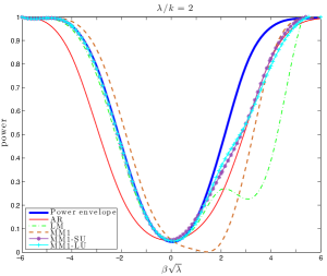
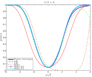
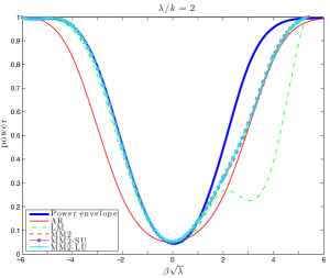
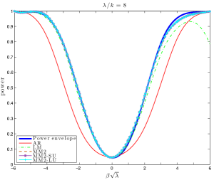
Figure 1 reports numerical results for the Kronecker product design. All four pictures present the power envelope and power curves for two existing tests, the Anderson-Rubin ($AR$) and score ($LM$) tests.

The first two graphs plot the power curves for the three WAP tests based on the MM1 statistic with $\sigma^{2}=10$. All three tests reject the null when the $h_{1}\left(s,t\right)$ statistic is larger than an adjusted critical value function. In practice, we approximate these critical value functions with 10,000 replications. The MM1 test sets the critical value function to be the 95% empirical quantile of $h_{1}\left(S,t\right)$. The MM1-SU test uses a conditional linear programming algorithm to find its critical value function. The MM1-LU test uses a nonlinear optimization package.

The AR test has power considerably lower than the power envelope when instruments are both weak ($\lambda/k=2$) and strong ($\lambda/k=8$). The LM test does not perform well when instruments are weak, and its power function is not monotonic even when instruments are strong. These two facts about the AR and LM tests are well documented in the literature; see Moreira (2003) and AMS06. The figure also reveals some salient findings for the tests based on the MM1 statistic. First, all MM1-based tests have correct size. Second, the MM1 similar test can have large bias to the point that it has zero power for parts of the parameter space. Hence, a naive choice for the density can yield a WAP test which can have overall poor power. We can eliminate this problem by imposing an unbiased condition when selecting an optimal test. The MM1-SU test is easy to implement and has power closer to the power upper bound. When instruments are weak, its power lies moderately below the reported power envelope. This is expected as the number of parameters is too large. When instruments are strong, its power is virtually the same as the power envelope.

To support the use of the MM1-SU test we also consider the MM1-LU test, which imposes a weaker unbiased condition. Close inspection of the graphs show that the derivative of the power function of the MM1 test is different from zero at $\beta=\beta_{0}$. This observation suggests that the power curve of the WAP test would change considerably if we were to force the power derivative to be zero at $\beta=\beta_{0}$. Indeed, we implement the MM1-LU test where the locally unbiased condition is true at only one point, the true parameter $\mu$. This parameter is of course unknown to the researcher and this test is not feasible. However, by considering the locally unbiased condition for other values of the instruments’ coefficients, the WAP test would be smaller —not larger. The power curves of MM1-LU and MM1-SU tests are very close, which shows that there is not much to be gained by relaxing the strongly unbiased condition.

The last two graphs plot the power curves for the three WAP tests based on the MM2 statistic with $\zeta=10$. By using the density $h_{2}\left(s,t\right)$, we avoid the pitfalls for the MM1 test. Recall that $h_{2}\left(s,t\right)$ is invariant to those data transformations which preserve the two-sided hypothesis testing problem. Hence, the MM2 similar test is unbiased and has overall good power without imposing any additional unbiased conditions. The graphs illustrate this theoretical finding, as the MM2, MM2-SU, and MM2-LU tests have numerically the same power curves. This conclusion changes dramatically when the covariance matrix is no longer a Kronecker product.

Figure 2: Power Comparison (Non-Kronecker Variance)

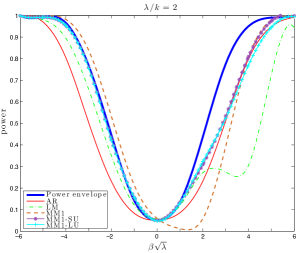
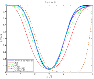
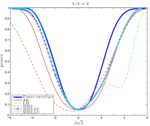
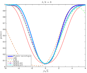
Figure 2 presents the power curves for all reported tests for the non-Kronecker design. Both MM1 and MM2 tests are severely biased and have overall bad power. For each design, we can make the tests approximately unbiased by choosing the $\sigma^{2}$ and $\zeta$ parameters large enough. However, this unbiasedness control is pointwise in the parameter space. We can always find a design such that each test behaves as a one-sided test and has very low power in parts of the parameter space. Hence, the strong asymptotic bias and often-low power of the conditional Wald tests found by Andrews, Moreira, and Stock (2007) also hold for the MM1 (even for the homoskedastic IV model) and MM2 similar tests (only for the HAC-IV model). These WAP similar tests are highly biased with power equal to zero in some parts of the parameter space. Therefore, just as Andrews, Moreira, and Stock (2007) object to the use of conditional Wald tests, we do not recommend the MM1 and MM2 similar tests for empirical researchers.

Proposition 2 shows that we cannot find a group of data transformations which preserve the two-sided testing problem with heteroskedastic-autocorrelated errors. Hence, a choice for the density for the WAP test based on symmetry considerations is not obvious. The correct density choice can be particularly difficult due to the large parameter-dimension (the coefficients $\mu$ and covariance $\Sigma$). Instead, we can endogenize the weight choice so that the WAP test will be automatically unbiased. This is done by the MM1-LU and MM2-LU tests. These two tests perform as well as the MM1-SU and MM2-SU tests. Because the latter two tests are easy to implement, we recommend their use in empirical practice.

6 Asymptotic Theory

All theoretical and numerical results so far do not rely on the sample size $n$ at all as we have assumed the statistics $S$ and $T$ to be exactly normally distributed with known variance $\Sigma$. In this section we relax this assumption at the cost of asymptotic approximations.

Let $z_{i}$ and $v_{i}$ denote the $i$-th row of $Z$ and $V$, respectively, written as column vectors of dimensions $k$ and $2$. We make the following two assumptions as the sample size $n$ grows.

Assumption 1. $n^{-1}Z^{\prime}Z=n^{-1}\sum_{i=1}^{n}z_{i}z_{i}^{\prime}\rightarrow_{p}D_{Z}$ for some positive definite $k\times k$ matrix $D_{Z}$.

Assumption 2. $n^{-1/2}\sum_{i=1}^{n}\left(v_{i}\otimes z_{i}\right)\rightarrow_{d}N(0,\Sigma_{\infty})$ for some positive definite $2k\times 2k$ matrix $\Sigma_{\infty}$.

Assumption 1 holds under Birkhoff’s Ergodic Theorem. Assumption 2 holds under suitable conditions by a central limit theorem (CLT). It also assumes that the long-run covariance matrix of $\Sigma_{\infty}$ is positive definite, as is usual in the literature. We no longer omit the dependence of $\Sigma$ on the sample size $n$ and, hereinafter, write $\Sigma_{n}$. Assumption 2 asserts that $\Sigma_{\infty}$ is the limit of $\Sigma_{n}$ as $n$ grows. Let $\widehat{\Sigma}_{n}$ be a consistent estimator of $\Sigma_{\infty}$ based on $\{\left(\widehat{v}_{i}\otimes z_{i}\right):i\leq n\}$, where $\widehat{v}_{i}$ are reduced-form residuals. There are many HAC estimators in the literature that can be used for this purpose; see, e.g., Newey and West (1987) and Andrews (1991). For brevity, we do not provide an explicit set of conditions under which one or more of these HAC estimators is consistent; see Jansson (2002) for details. We note, however, that the presence of weak instruments does not complicate standard proofs of the consistency of HAC estimators. Indeed, the convergence for most estimators holds uniformly over all true parameters $\beta$ and $\pi$.

We now introduce feasible versions of $S_{n}$ and $T_{n}$ with the variance $\Sigma_{n}$ replaced by the estimator $\widehat{\Sigma}_{n}$:

$$\widehat{S}_{n} = \left[\left(b_{0}^{\prime}\otimes I_{k}\right)\widehat{\Sigma}_{n}\left(b_{0}\otimes I_{k}\right)\right]^{-1/2}\left(b_{0}^{\prime}\otimes I_{k}\right)\overline{R}_{n}\text{ and}$$ (6.35)

$$\widehat{T}_{n} = \left[\left(a_{0}^{\prime}\otimes I_{k}\right)\widehat{\Sigma}_{n}^{-1}\left(a_{0}\otimes I_{k}\right)\right]^{-1/2}\left(a_{0}^{\prime}\otimes I_{k}\right)\widehat{\Sigma}_{n}^{-1}\overline{R}_{n},$$

where $\overline{R}_{n}=vec\left[\left(Z^{\prime}Z\right)^{-1/2}Z^{\prime}Y\right]$. Likewise, we define the feasible statistic $\widehat{\psi}_{n}$ as $\psi\left(S,T,\Sigma,D_{Z}\right)$ with the arguments being replaced by their sample analogues:

$$\widehat{\psi}_{n}=\psi(\widehat{S}_{n},\widehat{T}_{n},\widehat{\Sigma}_{n},\widehat{D}_{Z})\text{, where }\widehat{D}_{Z}=n^{-1}Z^{\prime}Z.$$ (6.36)

Assumption 3. The prior distribution for $\left(\beta,\pi\right)$ is absolutely continuous to the Lebesgue measure in $\mathbb{R}^{k+1}$. Its density

$$w(\beta,\pi,\widehat{D}_{Z})=w_{1}(\left.\pi\right|\beta,\widehat{D}_{Z})\cdot w_{2}(\beta,\widehat{D}_{Z})$$

has full support and is a continuous function of $\pi$ and $\beta$.

Assumption 3 allows the density $w(\beta,\pi,\widehat{D}_{Z})$ to depend on the data through $\widehat{D}_{Z}$. This generalization allows us to cover all tests considered here and asymptotically behaves as $w(\beta,\pi,D_{Z})$ (and so we will omit the dependence of the weights on $\widehat{D}_{Z}$ out of convenience). Although the conditional density $w_{1}(\left.\pi\right|\beta)$ does not depend on $\beta$ for the MM1 tests, it does depend on $\beta$ for the MM2 tests. Assumption 3 also guarantees that the priors for $\beta$ and $\pi$ are not dogmatic and will vanish asymptotically as in the Bernstein-von Mises theorem. If we set the prior on $\mu$, then the associated prior on $\pi$ $=\left(Z^{\prime}Z\right)^{1/2}\mu$ depends on the sample size. For example, the MM statistics introduced in (2.10) use the prior $\mu\sim N\left(0,\sigma^{2}\Phi\right)$. For the associated prior on $\pi\sim N\left(0,\left(\sigma^{2}/n\right)\widehat{D}_{Z}^{-1/2}\Phi\widehat{D}_{Z}^{-1/2}\right)$ not to be sensitive to the sample size, the parameters $\sigma^{2}$ and $\zeta$ present in the MM1 and MM2 statistics must eventually grow at the rate $n$. We make the dependence of $\Lambda\left(\beta,\mu\right)$ on the sample size $n$ explicit and, hereinafter, use the notation $\Lambda_{n}$.

We now analyze the asymptotic behavior of the WAP similar and WAP-SU tests. Recall that both of these types of tests depend on the test statistic

$$\frac{h_{\Lambda_{n}}\left(s,t\right)}{f_{\beta_{0}}^{S}\left(s\right)\cdot h_{\Lambda_{n}}^{T}\left(t\right)}.$$ (6.37)

When instruments are weak, the numerator and denominator have the same order of magnitude. When instruments are strong, the integrands in the weighted densities $h_{\Lambda_{n}}\left(s,t\right)$ and $h_{\Lambda_{n}}^{T}\left(t\right)$ grow exponentially fast and we can apply the Laplace approximation. Because both densities involve $k+1$ integrals, the test statistic in (6.37) is again well-behaved. The caveat is that a simple, closed-form approximation for $h_{\Lambda_{n}}^{T}\left(t\right)$ does not seem available under strong instruments. The WAP similar and WAP-SU tests, however, remain the same if we standardize (6.37) by any function of $t$. We replace $h_{\Lambda_{n}}^{T}\left(t\right)$ by $\left(1+\left\|t\right\|\right)^{-1}h_{\Lambda_{\beta_{0},n}}^{T}\left(t\right)$, where

$$h_{\Lambda_{\beta_{0},n}}^{T}\left(t\right)=\int f_{\beta_{0},\left(Z^{\prime}Z\right)^{1/2}\pi}^{T}\left(t\right)w\left(\beta_{0},\pi\right)d\pi.$$ (6.38)

The WAP similar and WAP-SU tests reject the null when

$$WAP=\frac{h_{\Lambda_{n}}\left(S,T\right)}{f_{\beta_{0}}^{S}\left(S\right)\cdot\left(1+\left\|T\right\|\right)^{-1}h_{\Lambda_{\beta_{0},n}}^{T}\left(T\right)}$$ (6.39)

is larger than $\kappa_{n}\left(t\right)$ and $\kappa_{n}\left(s,t\right)$, respectively.

Whether the instruments are weak or strong, we are able to obtain an approximation to (6.39). Define

$$n\cdot Q_{n}(\beta,\pi) = \frac{1}{2}\left\|\Sigma^{-1/2}\left(\overline{R}-(a\otimes\left(Z^{\prime}Z\right)^{1/2}\pi)\right)\right\|^{2}$$

$$= \frac{1}{2}\left\|[S:T]-\left[(\beta-\beta_{0})C_{\beta_{0}}:\text{ }D_{\beta}\right](I_{2}\otimes\left(Z^{\prime}Z\right)^{1/2}\pi)\right\|^{2}.$$

In Appendix B shows that the WAP statistic is asymptotically equivalent to

$$\frac{\int\exp\left(-n\cdot Q_{n}\left(\beta,\pi\left(\beta\right)\right)\right)w\left(\beta,\pi\left(\beta\right)\right)\left|\left(a^{\prime}\otimes\widehat{D}_{Z}^{1/2}\right)\Sigma_{n}^{-1}\left(a\otimes\widehat{D}_{Z}^{1/2}\right)\right|^{-1/2}d\beta}{\exp\left(-\frac{S^{\prime}S}{2}\right)\left[1+\left\|T\right\|\right]^{-1}w\left(\beta_{0},\pi\left(\beta_{0}\right)\right)\left|\left(a_{0}^{\prime}\otimes\widehat{D}_{Z}^{1/2}\right)\Sigma_{n}^{-1}\left(a_{0}\otimes\widehat{D}_{Z}^{1/2}\right)\right|^{-1/2}},$$ (6.40)

where the constrained maximum likelihood estimator (MLE) for $\pi$ is

$$\pi\left(\beta\right) = \left(Z^{\prime}Z\right)^{-1/2}\left[(a^{\prime}\otimes I_{k})\Sigma_{n}^{-1}(a\otimes I_{k})\right]^{-1}(a^{\prime}\otimes I_{k})\Sigma_{n}^{-1}\overline{R}\text{ and}$$ (6.41)

$$\overline{R} = \Sigma_{n}^{1/2}\left[\begin{array}[]{c}\left[\left(b_{0}^{\prime}\otimes I_{k}\right)\Sigma_{n}\left(b_{0}\otimes I_{k}\right)\right]^{-1/2}\left(b_{0}^{\prime}\otimes I_{k}\right)\Sigma_{n}^{1/2}\\ \left[\left(a_{0}^{\prime}\otimes I_{k}\right)\Sigma_{n}^{-1}\left(a_{0}\otimes I_{k}\right)\right]^{-1/2}\left(a_{0}^{\prime}\otimes I_{k}\right)\Sigma_{n}^{-1/2}\end{array}\right]^{\prime}\left[\begin{array}[]{c}S\\ T\end{array}\right].$$ (6.46)

The same approximation (6.40) holds for the $\widehat{WAP}$ statistic where we replace $S$, $T$, and $\Sigma$ by their feasible versions given in (6.35). The resulting approximation to the $\widehat{WAP}$ statistic is a function of $\widehat{S}_{n}$, $\widehat{T}_{n}$, $\Sigma_{n}$, and $\widehat{D}_{Z}$. The critical values for the WAP conditional tests and WAP-SU tests, respectively $\kappa_{n}\left(t\right)$ and $\kappa_{n}\left(s,t\right)$, are taken under the assumption that the $k$-dimensional vector $\widehat{S}_{n}$ has a standard normal distribution (in practice, these critical values are also functions of the consistent estimators $\widehat{\Sigma}_{n}$ and $\widehat{D}_{Z}$ as well, but we omit this dependence out of convenience). For example, for a given weight density $w\left(\beta,\pi\right)$, the critical function $\kappa_{n}\left(t\right)$ is simply the $1-\alpha$ quantile of (6.40) given $T=t$.

We now find the asymptotic distribution for the WAP tests under the WIV asymptotics. We make the following assumption.

Assumption WIV-FA. (a) $\pi=C/n^{1/2}$ for some non-stochastic vector $C$.

(b) $\beta$ is a fixed constant for all $n\geq 1.$

(c) $k$ is a fixed positive integer that does not depend on $n.$

Under WIV, $\pi\left(\beta\right)$ is $o_{p}\left(1\right)$ and the WAP statistics behave the same as if the weights were simply $w\left(\beta,0\right)$. As $n\rightarrow\infty$, the finite-sample critical value functions $\kappa_{n}\left(t\right)$ and $\kappa_{n}\left(s,t\right)$ respectively converge to their asymptotic counterparts $\kappa_{\infty}\left(t\right)$ and $\kappa_{\infty}\left(s,t\right)$, which are based on (6.40) with $w\left(\beta,\pi\left(\beta\right)\right)$ replaced by $w\left(\beta,0\right)$. We then obtain the following convergence by the continuous mapping theorem and the joint distribution

$$\left[\begin{array}[]{c}S_{\infty}\\ T_{\infty}\end{array}\right] \sim N\left(\left[\begin{array}[]{c}\left(\beta-\beta_{0}\right)C_{\beta_{0},\infty}\\ D_{\beta_{0},\infty}\end{array}\right]\left(D_{Z}\right)^{1/2}C,I_{2k}\right)\text{, where}$$ (6.51)

$$C_{\beta_{0},\infty} = \left[\left(b_{0}^{\prime}\otimes I_{k}\right)\Sigma_{\infty}\left(b_{0}\otimes I_{k}\right)\right]^{-1/2}\text{ and}$$

$$D_{\beta_{0},\infty} = \left[\left(a_{0}^{\prime}\otimes I_{k}\right)\Sigma_{\infty}^{-1}\left(a_{0}\otimes I_{k}\right)\right]^{-1/2}\left(a_{0}^{\prime}\otimes I_{k}\right)\Sigma_{\infty}^{-1}\left(a\otimes I_{k}\right).$$

Theorem 9.

Under Assumptions WIV-FA and 1-3:
(i) $\left(\widehat{S}_{n},\widehat{T}_{n}\right)\rightarrow_{d}\left(S_{\infty},T_{\infty}\right);$
(ii) $P\left(WAP\left(\widehat{S}_{n},\widehat{T}_{n}\right)>\kappa_{n}\left(\widehat{T}_{n}\right)\right)\rightarrow P\left(WAP\left(S_{\infty},T_{\infty}\right)>\kappa_{\infty}\left(T_{\infty}\right)\right);$ and
(iii) $P\left(WAP\left(\widehat{S}_{n},\widehat{T}_{n}\right)>\kappa_{n}\left(\widehat{S}_{n},\widehat{T}_{n}\right)\right)\rightarrow P\left(WAP\left(S_{\infty},T_{\infty}\right)>\kappa_{\infty}\left(S_{\infty},T_{\infty}\right)\right).$

Both WAP conditional and WAP-SU tests have asymptotic null rejection probabilities being equal to $\alpha$. The asymptotic power of the WAP tests has a complicated form under WIV asymptotics. We can, of course, rely on numerical simulations to compare their performance with other available tests. In Section 7, we present power plots for testing the intertemporal elasticity of substitution based on the designs of Yogo (2004).

For strong instruments with local alternatives (SIV-LA), we consider the Pitman drift where $\beta$ is local to the null value $\beta_{0}$ as $n\rightarrow\infty$.

Assumption SIV-LA. (a) $\beta=\beta_{0}+B/n^{1/2}$ for some constant $B\in\mathbb{R}.$

(b) $\pi$ is a fixed non-zero $k$-vector for all $n\geq 1.$

(c) $k$ is a fixed positive integer that does not depend on $n$.

Under the SIV-LA asymptotics, the WAP statistics are shown to be increasing transformations of the $LR$ statistic. This result is general and holds for any prior which satisfies Assumption 3.

Theorem 10.

Suppose Assumptions SIV-LA and 1-3 hold. The long-run variance $\Sigma_{\infty}$ is known, or unknown but consistently estimable by $\widehat{\Sigma}_{n}$. Then the WAP similar and WAP-SU tests are asymptotically equivalent to the LR test given in (2.6).

Comment. 1. In the proof, we apply the Laplace approximation twice, first with respect to the integral for $\pi$ and then for $\beta$. For the MM1 and MM2 statistics, we can alternatively find a simple expression after integrating out the prior for the instruments’ coefficients with $\sigma^{2}$ or $\zeta$ growing at rate $n$ and then applying the Laplace approximation for $\beta$. Both approaches coincide.

2. The SIV-LA behavior of the ECS (HAC-IV) test appears to be just a special case of our theory using Laplace approximations.

3. For higher-order expansions, we can use Watson’s lemma; for references, we recommend Olver (1997) for deterministic functions and Onatski, Moreira, and Hallin (2014a, 2014b) for random functions.

4. Because $T_{n}/n^{1/2}\rightarrow_{p}D_{\beta_{0}}D_{Z}^{1/2}\pi$ under SIV-LA, $\left\|T_{n}\right\|$ diverges to infinity w.p.1 (with probability approaching one). The critical value functions for both the WAP conditional and WAP-SU tests collapse then to the $1-\alpha$ asymptotic (unconditional) quantile. As a result, the WAP conditional and WAP-SU tests are asymptotically similar and efficient under the SIV asymptotics.

The null rejection probability of WAP tests is $\alpha$ under WIV and SIV asymptotics. Pointwise convergence of the null rejection probability, of course, does not necessarily imply the size is asymptotically $\alpha$ (in a uniform sense). Moreira (2003, p. 1037) suggests to use Parzen (1954) and Andrews (1986) to assure size is uniformly controlled. A series of papers, including Andrews, Cheng, and Guggenberger (2011) and Andrews and Guggenberger (2014a), develop several powerful methods to check uniform size control and have been applied to many econometric models; see Andrews and Guggenberger (2010), Andrews and Guggenberger (2014a), and Mills, Moreira, and Vilela (2014b), among others. Conceivably, we can apply those methods to the WAP statistics coupled with the critical value functions $\kappa_{n}\left(t\right)$ and $\kappa_{n}\left(s,t\right)$. This line of research will be considered in a separate paper.

We can also analyze the WAP tests under strong instruments with fixed alternatives (SIV-FA). We follow Mills, Moreira, and Vilela (2014a) and make the following assumption.

Assumption SIV-FA. (a) $\beta=\beta_{0}+B$ for some nonzero $B\in\mathbb{R}.$

(b) $\pi$ is a fixed non-zero $k$-vector for all $n\geq 1.$

(c) $k$ is a fixed positive integer that does not depend on $n$.

It is natural to expect that the power converges to one if the parameter $\beta$ is fixed. However, not all tests have this property even in the IV model with homoskedastic errors; see Andrews, Moreira, and Stock (2004) and Mills, Moreira, and Vilela (2014a) for examples. Hence, it is important to establish consistency for the WAP tests.

If the parameter $\beta$ is fixed, the WAP statistics are proportional to the exponential of $LR$. Because $LR/n$ converges to a non-zero constant, the WAP tests are consistent. The next theorem formalizes this result.

Theorem 11.

Suppose Assumptions SIV-FA and 1-3 hold. The long-run variance $\Sigma_{\infty}$ is known, or unknown but consistently estimable by $\widehat{\Sigma}_{n}$. Then the following hold:
(i) $2.\left(\log\widehat{WAP}\right)/n=\widehat{LR}/n+o_{p}\left(1\right);$ and
(ii) $\widehat{LR}/n=LR/n+o_{p}\left(1\right)\rightarrow\gamma>0.$

Comment: If $D_{\beta}\neq 0$, the functions $\kappa_{n}\left(t\right)$ and $\kappa_{n}\left(s,t\right)$ converge to a constant obtained under SIV-FA. If $D_{\beta}=0$, the critical functions do not converge. However, they are bounded, and so WAP tests are consistent.

7 Power Comparison

In this section, we follow I. Andrews (2015) who calibrates designs for power comparison based on the work of Yogo (2004) on the elasticity of intertemporal substitution in eleven developed countries.

Yogo (2004) tests the effect of interest rates on the level of aggregate demand in an IV model. He considers a linear regression in which asset return affects consumption growth, and the reverse form of this regression. In both equations, the endogenous variable (consumption or asset return) can be correlated with the error (innovation). To remedy this problem, he chooses four instruments: lagged values of nominal interest rate, inflation, consumption growth, and log dividend-price ratio.

I. Andrews (2015) selects the real interest rate (rf in Yogo’s (2004) notation) as the endogenous variable. Several tests perform well in his design, including MM2-SU, PI-CLC, and (WAP similar) ECS tests. In fact, only in a few countries do these tests have slightly different performance; see Section 7.2.1 of I. Andrews (2015). The difficulty in assessing the relative performance of each test arises because the instruments are not particularly weak in this design. Indeed, the first-stage F-statistic reported by Yogo (2004) (see his Table I) is below 10 in only four countries (Japan, Switzerland, United Kingdom, and the United States). We instead join de Castro (2015) in choosing the real stock return (re in Yogo’s (2004) notation) as the endogenous variable. The instruments are considerably weaker in this design: the F-statistic is smaller than 4.18 in all countries, and always less than the F-statistic for interest rate. Our decision to use stock returns aims to highlight the differences between the tests proposed for the HAC-IV model. Apart from using stock returns instead of interest rates, our design is akin to that of I. Andrews (2015). We use the Newey-West estimator with three lags, and the resulting power curves are based on 5,000 Monte Carlo simulations. In parallel to our asymptotic theory, we choose the ratio of the tuning parameters $\sigma^{2}$ and $\zeta$ to the sample size to be one-tenth for the MM1 and MM2 statistics, respectively.

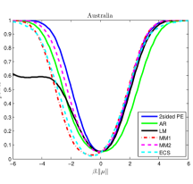
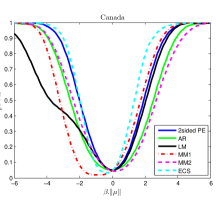
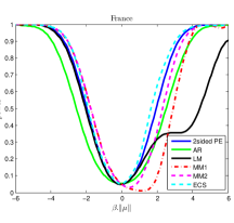
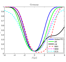
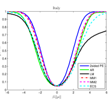
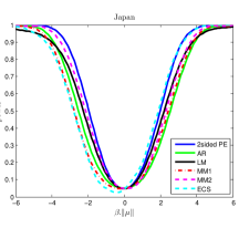
Figure 3 plots power curves for the two-sided power envelope, Anderson-Rubin (AR), score (LM), WAP similar MM1, WAP similar MM2, and ECS (HAC-IV) tests. Although the AR and LM tests are unbiased, the MM1, MM2, and ECS tests perform unreliably. To illustrate the problem, we mention three countries. For Australia, the MM1 and ECS tests have low power for parts of the parameter space, while the MM2 test behaves more like a two-sided test. For France, the ECS test performs well, while both MM1 and MM2 tests can have low power. For the USA, the ECS test has power near zero and behaves more as a one-sided test while the MM1 and MM2 tests are nearly unbiased. In some countries, these three tests have power even lower than the Anderson-Rubin test (e.g., the ECS test for Germany and Italy).

Figure 3: Power Comparison (WAP similar tests)

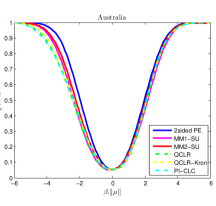
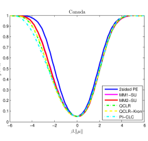
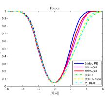
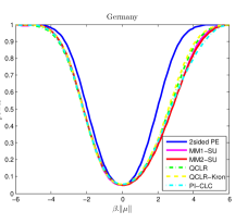
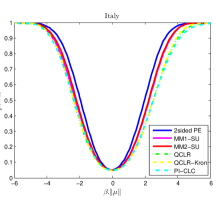
We then compare power among two-sided tests which have arguably better performance. Figure 4 plots power curves for the two-sided power envelope, MM1-SU, MM2-SU, CQLR, CQLR-kron, and PI-CLC tests. All tests are adequate for two-sided hypothesis testing. The PI-CLC and CQLR-kron test show some improvements over the CQLR test for some, but not all, countries. The MM1-SU test behaves near the MM2-SU test for several countries, but it has considerably lower power for Japan and the United States. The MM2-SU test outperforms these tests and when it occasionally has less power, the power loss is small. This application based on real data supports our theoretical contribution and the use of the MM2-SU test in practice.

Figure 5: Power Comparison (two-sided tests)

8 Concluding Remarks

In this paper, we study the instrumental variable (IV) model with one endogenous regressor and heteroskedastic and autocorrelated (HAC) errors. The HAC-IV model with a known variance matrix is simpler than the model with an unknown but consistently estimable long-run variance. However, inference in both models is approximately the same whether or not the instruments are weakly correlated with the endogenous variable. This simplification allows us to develop a theory of optimal two-sided tests when the error stochastic process is of unknown form.

We find that a test that has correct size and is optimal under standard asymptotics may still have unacceptably low power in finite samples. This issue appears in several econometric models. For the HAC-IV model, we solve this problem by finding weighted-average power tests satisfying additional two-sided conditions. In this paper, we consider two possibilities: the locally unbiased (LU) and strongly unbiased (SU) conditions. While the local condition yields admissible tests, the stronger condition is easier to implement. Better yet, the MM1-SU and MM2-SU tests have power numerically very close to their LU versions. Numerical simulations also show that the MM2-SU test outperforms other tests proposed for the HAC-IV model.

The only other paper that satisfactorily addresses optimality of two-sided tests in the HAC-IV model is that of I. Andrews (2015). He explores linear combinations of the Anderson-Rubin and score statistics, with weights dependent on the conditioning statistic $T$. A class of these conditional linear combination (CLC) tests is unbiased and admissible in the conditional problem. By proposing a minimax regret criterion, he delivers a test which plugs in a nuisance-parameter estimator. There is some power gained by broadening the focus beyond those three statistics. On the other hand, we impose $k$ additional constraints which are related to the SU condition. It would be interesting to reduce the required computational time while maintaining the power gains of the MM2-SU test by reducing the number of boundary conditions when finding a WAP test.

Finally, the asymptotic theory based on Laplace approximations, developed in this paper, is easily adaptable to other econometric models. For the HAC-IV model, it relies on priors for the parameters $\beta$ and $\pi$ being insensitive to the sample size. For the MM1 and MM2 weights, this implies that the tuning parameters $\sigma^{2}$ and $\zeta$ (used in the prior for $\mu=\left(Z^{\prime}Z\right)^{1/2}\pi$) eventually grow at the sample size $n$. Some power gains with weak instruments may be possible when the tuning parameters are held constant. Another alternative is to find an automatic rate for $\sigma^{2}$ and $\zeta$ using a plug-in method. For example, we could let these parameters be proportional to either $\left\|T\right\|^{2}$ or $n\cdot\left\|\pi\left(\beta_{0}\right)\right\|^{2}$. These quantities are stochastically bounded under weak instruments and grow at the rate $n$ under strong instruments (which assures asymptotic optimality). Since the constrained MLE $\pi\left(\beta_{0}\right)$ is a one-to-one transformation of $T$, these modifications of WAP-SU tests are still similar and uncorrelated with the pivotal statistic $S$ (hence, satisfy the SU Condition). We will consider this possibility in future work.

References

- (1)
- Anderson and Rubin (1949) Anderson, T. W., and H. Rubin (1949): “Estimation of the Parameters of a Single Equation in a Complete System of Stochastic Equations,” Annals of Mathematical Statistics, 20, 46–63.
- Andrews (1986) Andrews, D. W. K. (1986): “Complete Consistency: A Testing Analogue of Estimator Consistency,” The Review of Economic Studies, 53, 263–269.
- Andrews (1991) Andrews, D. W. K. (1991): “Heteroskedasticity and Autocorrelation Consistent Covariance Matrix Estimation,” Econometrica, 59, 817–858.
- Andrews, Cheng, and Guggenberger (2011) Andrews, D. W. K., X. Cheng, and P. Guggenberger (2011): “Generic Results for Establishing the Asymptotic Size of Confi dence Sets and Tests,” Tests, Cowles Foundation Discussion Papers 1813, Cowles Foundation for Research in Economics, Yale University.
- Andrews and Guggenberger (2010) Andrews, D. W. K., and P. Guggenberger (2010): “Applications of Subsampling, Hybrid, and Size-Correction Methods,” Journal of Econometrics, 158, 285–305.
- Andrews and Guggenberger (2014a) (2014a): “Asymptotic Size of Kleibergen’s LM and Conditional LR Tests for Moment Condition Models,” Working paper, Yale University.
- Andrews and Guggenberger (2014b) (2014b): “Identifi cation- and Singularity-Robust Inference for Moment Condition Models,” Working paper, Yale University.
- Andrews, Moreira, and Stock (2004) Andrews, D. W. K., M. J. Moreira, and J. H. Stock (2004): “Optimal Invariant Similar Tests for Instrumental Variables Regression,” NBER Working Paper t0299.
- Andrews, Moreira, and Stock (2006a) (2006a): “Optimal Two-Sided Invariant Similar Tests for Instrumental Variables Regression,” Econometrica, 74, 715–752.
- Andrews, Moreira, and Stock (2006b) (2006b): “Optimal Two-Sided Invariant Similar Tests for Instrumental Variables Regression,” Econometrica, 74, 715–752, Supplement.
- Andrews, Moreira, and Stock (2007) (2007): “Performance of Conditional Wald Tests in IV Regression with Weak Instruments,” Journal of Econometrics, 139, 116–132.
- Andrews (2015) Andrews, I. (2015): “Conditional Linear Combination Tests for Weakly Identified Models,” Unpublished Manuscript, MIT.
- Andrews and Mikusheva (2015) Andrews, I., and A. Mikusheva (2015): “Conditional Inference with a Functional Nuisance Parameter,” Working paper, MIT.
- Bound, Jaeger, and Baker (1995) Bound, J., D. A. Jaeger, and R. M. Baker (1995): “Problems with Instrumental Variables Estimation When the Correlation Between the Instruments and the Endogenous Explanatory Variables is Weak,” Journal of American Statistical Association, 90, 443–450.
- de Castro (2015) de Castro, G. R. (2015): “Invariant Tests in an Instrumental Variables Model with Unknown Data Generating Process,” Master’s thesis, FGV/EPGE.
- Dufour (1997) Dufour, J.-M. (1997): “Some Impossibility Theorems in Econometrics with Applications to Structural and Dynamic Models,” Econometrica, 65, 1365–1388.
- Edwards (1992) Edwards, A. W. F. (1992): Likelihood. John Hopkins University Press, Baltimore.
- Elliott, Mueller, and Watson (2015) Elliott, G., U. Mueller, and M. Watson (2015): “Nearly Optimal Tests When a Nuisance Parameter Is Present Under the Null Hypothesis,” Econometrica, 83, 771–811.
- Guggenberger and Smith (2005) Guggenberger, P., and R. Smith (2005): “Generalized Empirical Likelihood Estimators and Tests Under Partial, Weak and Strong Identification,” Econometric Theory, 21, 667–709.
- Jansson (2002) Jansson, M. (2002): “Consistent Covariance Matrix Estimation for Linear Processes,” Econometric Theory, 18, 1449–1459.
- Kleibergen (2002) Kleibergen, F. (2002): “Pivotal Statistics for Testing Structural Parameters in Instrumental Variables Regression,” Econometrica, 70, 1781–1803.
- Kleibergen (2006) (2006): “Testing Parameters in GMM Without Assuming That They Are Identifi ed,” Econometrica, 73, 1103–1123.
- Lehmann (1952) Lehmann, E. L. (1952): “On the Existence of Least Favorable Distributions,” Annals of Mathematical Statistics, 23, 408–416.
- Lehmann and Romano (2005) Lehmann, E. L., and J. P. Romano (2005): Testing Statistical Hypotheses. Third edn., Springer Series in Statistics.
- Mills, Moreira, and Vilela (2014a) Mills, B., M. J. Moreira, and L. P. Vilela (2014a): “Tests Based on t-Statistics for IV Regression with Weak Instruments,” Journal of Econometrics, 182, 351–363.
- Mills, Moreira, and Vilela (2014b) (2014b): “Tests Based on t-Statistics for IV Regression with Weak Instruments,” Journal of Econometrics, 182, 351–363, Supplement.
- Moreira and Moreira (2010) Moreira, H., and M. J. Moreira (2010): “Contributions to the Theory of Similar Tests,” Working Paper, FGV/EPGE.
- Moreira and Moreira (2013) (2013): “Contributions to the Theory of Optimal Tests,” Ensaios Economicos, 747, FGV/EPGE.
- Moreira (2001) Moreira, M. J. (2001): “Tests with Correct Size when Instruments Can Be Arbitrarily Weak,” Center for Labor Economics Working Paper Series, 37, UC Berkeley.
- Moreira (2002) (2002): “Tests with Correct Size in the Simultaneous Equations Model,” Ph.D. thesis, UC Berkeley.
- Moreira (2003) (2003): “A Conditional Likelihood Ratio Test for Structural Models,” Econometrica, 71, 1027–1048.
- Moreira (2009) (2009): “Tests with Correct Size when Instruments Can Be Arbitrarily Weak,” Journal of Econometrics, 152, 131–140.
- Nelson and Startz (1990) Nelson, C. R., and R. Startz (1990): “Some Further Results on the Exact Small Sample Properties of the Instrumental Variable Estimator,” Econometrica, 58, 967–976.
- Newey and West (1987) Newey, W. K., and K. D. West (1987): “A Simple, Positive Semi-Definite, Heteroskedasticity and Autocorrelation Consistent Covariance Matrix,” Econometrica, 55, 703–708.
- Olea (2015) Olea, J. L. M. (2015): “Efficient Conditionally Similar Tests: Finite-Sample Theory and Large-Sample Applications,” Working paper, NYU.
- Olver (1997) Olver, F. W. J. (1997): Asymptotics and Special Functions. San Diego, Academic Press.
- Onatski, Moreira, and Hallin (2014a) Onatski, A., M. J. Moreira, and M. Hallin (2014a): “Asymptotic Power of Sphericity Tests for High-Dimensional Data,” Annals of Statistics, 41, 1204–1231.
- Onatski, Moreira, and Hallin (2014b) (2014b): “Signal Detection in High Dimension: The Multispiked Case,” Annals of Statistics, 42, 225–254.
- Otsu (2006) Otsu, T. (2006): “Generalized Empirical Likelihood Inference for Nonlinear and Time Series Models Under Weak Identification,” Econometric Theory, 22, 513–527.
- Parzen (1954) Parzen, E. (1954): “On Uniform Convergence of Families of Sequences of Random Variables,” University of California Publications in Statistics, 2, 23–54.
- Staiger and Stock (1997) Staiger, D., and J. H. Stock (1997): “Instrumental Variables Regression with Weak Instruments,” Econometrica, 65, 557–586.
- Stock and Wright (2000) Stock, J. H., and J. Wright (2000): “GMM with Weak Identification,” Econometrica, 68, 1055–1096.
- Van Loan and Ptsianis (1993) Van Loan, C., and N. Ptsianis (1993): “Approximation with Kronecker Products,” in Linear Algebra for Large Scale and Real-Time Applications, ed. by M. Moonen, and G. Golub, pp. 293–314. Springer, Leuven.
- Yogo (2004) Yogo, M. (2004): “Estimating the Elasticity of Intertemporal Rate of Substitution When Instruments Are Weak,” Review of Economics and Statistics, 86, 797–810.