Is the small-scale magnetic field correlated with the dynamo cycle?

Abstract

The small-scale magnetic field is ubiquitous at the solar surface—even at high latitudes. From observations we know that this field is uncorrelated (or perhaps even weakly anticorrelated) with the global sunspot cycle. Our aim is to explore the origin, and particularly the cycle dependence of such a phenomenon using three-dimensional dynamo simulations. We adopt a simple model of a turbulent dynamo in a shearing box driven by helically forced turbulence. Depending on the dynamo parameters, large-scale (global) and small-scale (local) dynamos can be excited independently in this model. Based on simulations in different parameter regimes, we find that, when only the large-scale dynamo is operating in the system, the small-scale magnetic field generated through shredding and tangling of the large-scale magnetic field is positively correlated with the global magnetic cycle. However, when both dynamos are operating, the small-scale field is produced from both the small-scale dynamo and the tangling of the large-scale field. In this situation, when the large-scale field is weaker than the equipartition value of the turbulence, the small-scale field is almost uncorrelated with the large-scale magnetic cycle. On the other hand, when the large-scale field is stronger than the equipartition value, we observe an anticorrelation between the small-scale field and the large-scale magnetic cycle. This anticorrelation can be interpreted as a suppression of the small-scale dynamo. Based on our studies we conclude that the observed small-scale magnetic field in the Sun is generated by the combined mechanisms of small-scale dynamo and tangling of the large-scale field.

1. Introduction

Sunspots and the solar cycle are associated with the large-scale magnetic field of the Sun. This magnetic field is believed to be produced by a large-scale dynamo, globally operating in the solar convection zone. The $\alpha$ effect (originating either from helical flow and/or the Babcock-Leighton process) and the $\Omega$ effect (shearing of the magnetic field by differential rotation) are believed to be the cause of this dynamo in the Sun (see reviews by Charbonneau, 2014; Karak et al., 2014). However, there is another type of magnetic field that exists at small scales and even in the quiet phase of the Sun. This field is intermittent and fluctuating and exists in mixed polarity even at the resolution limits of present day instruments. This field is known as small-scale, fluctuating, turbulent, or internetwork field—as it exists in the internetwork regions. Although the existence of this field has been known for a long time (e.g., Howard & Stenflo, 1972; Frazier & Stenflo, 1972), the detailed understanding of its nature and origin has remained elusive. The main reason for this is that the spatial characteristic scale of this field is shorter than the resolution limits of present day instruments and the weak polarization signal makes the measurement of this quiet-Sun magnetic field difficult (e.g., de Wijn et al., 2009). Interestingly, even the internetwork field—the weakest component of solar magnetism—having an unsigned flux of $\approx 10^{15}-10^{18}\,{\rm Mx}$, contributes about $10^{26}$ Mx of magnetic flux to the solar surface per day, which is at least four orders of magnitude more than that from the bipolar active regions (which contain an unsigned flux of $\approx 5\times 10^{20}-5\times 10^{22}\,{\rm Mx}$) during solar maximum (Schrijver & Harvey, 1994; Zhou et al., 2013). In comparison, both the network regions with a flux of $\approx 10^{17}-10^{19}\,{\rm Mx}$ and ephemeral regions with $10^{18}-5\times 10^{20}\,{\rm Mx}$ contribute roughly two orders of magnitude more flux than active regions (Hagenaar et al., 2003; Gošić et al., 2014). Therefore, the small-scale magnetic field is potentially important in understanding many unsolved problems in solar physics, particularly solar atmospheric heating (e.g., Schrijver et al., 1998).

Since Batchelor (1950) it is known that a sufficiently random three-dimensional velocity field can amplify a seed magnetic field via repeated random stretching, bending and folding—without requiring net helicity. This is the essence of the small-scale or local dynamo. The correct mathematical description of such dynamos was developed later by Kazantsev (1968); see also Childress & Gilbert (1995). Petrovay & Szakaly (1993) were the first to realize the necessity of a small-scale dynamo to explain the magnetic flux budget in the photosphere (also see Durney et al., 1993). However, one may put forward alternative arguments in which this quiet-Sun magnetic field is the result of a global large-scale dynamo: the shredding of large-scale magnetic field can produce small-scale magnetic field by cascading magnetic energy to small-scales and the decay of active regions may give rise to small-scale magnetic field (Spruit et al., 1987; de Wijn et al., 2005; Stenflo, 2012). However, none of these arguments may necessarily be correct because the small-scale magnetic field does not show solar cycle dependence, as it does not have significant correlation with the large-scale global magnetic cycle, and it does not have much latitudinal variation (e.g., Hagenaar et al., 2003; Sánchez Almeida, 2003; Lites et al., 2008; Lites, 2011; Buehler et al., 2013; Jin & Wang, 2015b). Furthermore, using the MDI data set of the entire solar cycle 23, Jin et al. (2011) have shown that the cyclic variation of both number and total flux of small-scale magnetic elements in the range $\sim(3$–$30)\times 10^{18}\,{\rm Mx}$ are anticorrelated with the sunspot number. Subsequently, Jin & Wang (2015a) have studied the internetwork magnetic field within the flux range of about $10^{16}$–$10^{18}\,{\rm Mx}$ and find no correlation with the solar cycle. All these observational results support the small-scale dynamo scenario as the source of small-scale field in the Sun. We note that Sokoloff et al. (2015) argued in favor of the operation of a small-scale dynamo in the Sun to explain the observational findings that the number of anti-Hale sunspot groups becomes maximal during solar minimum and that these groups do not show the latitudinal dependence as Hale sunspots.

The complex nature of the stratified convection zone with very low values of molecular viscosity, diffusivity, and magnetic Prandtl number ($P_{\rm m}$) make the theoretical modeling of the small-scale field challenging at present. Furthermore, at small $P_{\rm m}$, the critical magnetic Reynolds number, $R_{\rm m}^{C}$ needed to excite the small-scale dynamo increases at first linearly with deceasing $P_{\rm m}$ (Rogachevskii & Kleeorin, 1997; Boldyrev & Cattaneo, 2004; Schekochihin et al., 2005) until $R_{\rm m}^{C}$ saturates for $P_{\rm m}\ll 1$ (Iskakov et al., 2007; Brandenburg, 2011), which makes the small-scale dynamo at the solar value of $P_{\rm m}\sim 10^{-5}$ possible. Beside these difficulties several authors (e.g., Cattaneo, 1999; Emonet & Cattaneo, 2001) tried to model the small-scale dynamo in a local Cartesian box. Although they found in some cases small-scale dynamo action, these simulations are highly idealized and far from the real Sun. Subsequently, Vögler et al. (2005) (see also Vögler & Schüssler, 2007; Pietarila Graham et al., 2010; Rempel, 2014) have gone one step further to make these models more realistic by including radiation and ionization. However, these simulations are local in the sense that they cannot study the effects of the global dynamo-generated large-scale field on the small-scale field. Very recently, Hotta et al. (2014, 2015) have studied small-scale dynamo action in the Sun using high-resolution MHD simulations. Again, however, these simulations did not consider the large-scale dynamo.

The purpose of the present study is to explore the effects of a global dynamo-generated cyclic large-scale magnetic field on the small-scale field. To this end, we perform a set of simulations of a turbulent cyclic dynamo that produces a migratory magnetic field similar to that of the Sun. To capture the essential features of an $\alpha\Omega$ dynamo, in particular its migratory properties, we employ helically forced turbulence together with imposed uniform shear across the domain. These two ingredients provide a prototype of an $\alpha\Omega$ dynamo, as it is often modelled in mean-field theory. Earlier turbulence simulations of this type have confirmed the presence of cyclic solutions with dynamo waves whose direction of propagation depends on the sign and magnitude of shear and helicity (Käpylä & Brandenburg, 2009; Karak et al., 2015b).

We do not make an attempt to model the real Sun, whose underlying dynamo mechanism is still not well understood (Brandenburg, 2005; Charbonneau, 2014). It is not even completely clear whether the solar dynamo is driven by convective motions or by magnetic instabilities (Brandenburg, 1998; Tobias et al., 2011), and whether meridional circulation plays an important role for causing the equatorward migration of the Sun’s magnetic field (Choudhuri et al., 1995; Hazra et al., 2014). Furthermore, we are facing even more fundamental challenges, for example the question of catastrophic quenching, the dependence of mean field strength on magnetic Reynolds number, and the morphology of the field in the form of tubes on the one hand, and the question of magnetic buoyancy, flux tube storage, and sunspot formation on the other. Significant progress has been made by considering these aspects separately, since in models with all effects included it is difficult to associate particular features to given changes in the model. Thus, in our model, we focus on the aspect of large-scale and small-scale dynamos only, i.e., we do not consider the question of magnetic buoyancy, flux tube storage, and sunspot formation. Consequently, we consider a model without gravity and convection and consider turbulence to be driven by a stochastic forcing. Moreover, our simple model then avoids the vastly different time and length scales of global and local dynamos in realistic settings. Capturing them within a single model remains a challenging task in global convection simulations (Vögler et al., 2005; Käpylä et al., 2013; Karak et al., 2015a; Hotta et al., 2015). In the present paper, our aim is to address the basic question whether and how the small-scale magnetic field is correlated with the dynamo cycle in a simple realization of a turbulent dynamo that combines the physics of a small-scale dynamo with that of an $\alpha\Omega$ dynamo.

2. Model

In this work we do not consider convection. Therefore, gravitational stratification and thermodynamics are neglected. Instead, our model consists of an isothermal, compressible fluid where the pressure is given by $p=c_{\rm s}^{2}\rho$, with $c_{\rm s}$ being the isothermal (constant) sound speed and $\rho$ the density. We sustain turbulence by supplying energy to the system through a stochastic forcing function in the momentum equation. As we do not include the stratification and global rotation of the Sun, we make this forcing helical to produce an $\alpha$ effect in our model. Furthermore, to mimic the large-scale shear of the Sun and to produce an $\Omega$ effect, we impose a uniform shear flow in our model. We solve the hydromagnetic equations in a cubic domain of size $(2\pi)^{3}$. To connect with spherical geometry, we can imagine our simulation box being located in the northern hemisphere of the Sun such that the $x$ axis corresponds to the radially outward direction, the $y$ axis to the toroidal direction, and the $z$ axis to the direction of increasing latitude; see, e.g., Käpylä et al. (2013), who used the same correspondence in their Section 3.6. Within this framework, the momentum, continuity, and induction equations become

$$\frac{D\mbox{\boldmath$U$}{}}{Dt}=\mbox{\boldmath$f$}{}-SU_{x}\hat{y}-c_{\rm s}^{2}\mbox{\boldmath$\nabla$}{}\ln\rho+\frac{1}{\rho}\left[\mbox{\boldmath$J$}{}\times\bm{B}+\mbox{\boldmath$\nabla$}{}\!\cdot(\!2\rho\nu\mbox{\boldmath${\sf S}$}{})\right],\;$$ (1)

$$\frac{D\ln\rho}{Dt}=-\mbox{\boldmath$\nabla$}{}\cdot\mbox{\boldmath$U$}{},$$ (2)

$$\frac{\partial\mbox{\boldmath$A$}{}}{\partial t}+\mbox{\boldmath$U$}{}^{(S)}\cdot\mbox{\boldmath$\nabla$}{}\mbox{\boldmath$A$}{}=-SA_{y}\hat{x}+\mbox{\boldmath$U$}{}\times\bm{B}+\eta\mbox{\boldmath$\nabla$}{}^{2}\mbox{\boldmath$A$}{},$$ (3)

where $D/Dt=\partial/\partial t+(\mbox{\boldmath$U$}{}+\mbox{\boldmath$U$}{}^{(S)})\cdot\bm{\mbox{\boldmath$\nabla$}{}}$ is the advective time derivative, $\mbox{\boldmath$U$}{}^{(S)}=(0,Sx,0)$ is the imposed uniform large-scale shear flow with $S$ being the constant shear rate, $\textstyle f$ is the forcing function that we describe later, $\nu$ is the constant kinematic viscosity, and ${\sf S}$ is the traceless rate of strain tensor given by ${\sf S}_{ij}={\textstyle{1\over 2}}(U_{i,j}+U_{j,i})-{\textstyle{1\over 3}}\delta_{ij}\bm{\nabla}\cdot\bm{U}$ (the commas denote partial differentiation with respect to the coordinate $j$ or $i$). The contribution of $\mbox{\boldmath$U$}{}^{(S)}$ to the viscous stress is small compared with that of $U$ and is neglected. We note that the induction equation is written in terms of the magnetic vector potential $A$, such that $\mbox{\boldmath$\nabla$}{}\times{\mbox{\boldmath$A$}{}}$ = ${\bm{B}}$ is the magnetic field. Furthermore, $\mbox{\boldmath$J$}{}=\mu_{0}^{-1}\mbox{\boldmath$\nabla$}{}\times\bm{B}$ is the current density, and $\eta$ is the constant microscopic diffusivity

The forcing function $\mathchoice{\mbox{\boldmath$\displaystyle f$}}{\mbox{\boldmath$\textstyle f$}}{\mbox{\boldmath$\scriptstyle f$}}{\mbox{\boldmath$\scriptscriptstyle f$}}=\mathchoice{\mbox{\boldmath$\displaystyle f$}}{\mbox{\boldmath$\textstyle f$}}{\mbox{\boldmath$\scriptstyle f$}}{\mbox{\boldmath$\scriptscriptstyle f$}}(\bm{x},t)$ in Equation (1) is helical and random in time. It is defined as $\mbox{\boldmath$f$}{}(\bm{x},t)={\rm Re}\{N\mbox{\boldmath$f$}{}_{\bm{k}(t)}\exp[{\rm i}\bm{k}(t)\cdot\bm{x}+{\rm i}\phi(t)]\},$ where $\bm{x}$ is the position vector. At each timestep, the wavevector $\bm{k}(t)$ randomly takes any value from all possible wavevectors in a certain range around a given forcing wavenumber $k_{\rm f}$. The phase $-\pi<\phi(t)\leq\pi$ also changes randomly at every timestep. On dimensional grounds, we choose $N=f_{0}c_{\rm s}(|\bm{k}|c_{\rm s}/\delta t)^{1/2}$, where $f_{0}$ is a non-dimensional forcing amplitude. The transverse helical waves are produced via Fourier amplitudes (Haugen et al., 2004)

$$\mbox{\boldmath$f$}{}_{\bm{k}}=\mbox{\boldmath${\sf R}$}{}\cdot\mbox{\boldmath$f$}{}_{\bm{k}}^{\rm(nohel)}\quad\mbox{with}\quad{\sf R}_{ij}={\delta_{ij}-{\rm i}\sigma\epsilon_{ijk}\hat{k}_{k}\over\sqrt{1+\sigma^{2}}},$$ (4)

where $\sigma$ is a measure of the helicity of the forcing; for positive maximum helicity, $\sigma=1$, $\mbox{\boldmath$f$}{}_{\bm{k}}^{\rm(nohel)}=\left(\bm{k}\times\hat{\mbox{\boldmath$e$}}{}\right)/\sqrt{\bm{k}^{2}-(\bm{k}\cdot\hat{\mbox{\boldmath$e$}}{})^{2}},$ where $\hat{\mbox{\boldmath$e$}}{}$ is an arbitrary unit vector not aligned with $\bm{k}$. Note that $|\mbox{\boldmath$f$}{}_{\bm{k}}|^{2}=1$ and $\mbox{\boldmath$f$}{}_{\bm{k}}\cdot({\rm i}\bm{k}\times\mbox{\boldmath$f$}{}_{\bm{k}})^{*}=2\sigma k/(1+\sigma^{2})$.

We solve the above equations with the Pencil Code in $-\pi<x,y,z<\pi$ with boundary conditions that are shearing–periodic in the $x$ direction and periodic in the $y$ and $z$ directions. The numerical time step $\Delta t$ is computed as the Courant time step. As initial conditions we take $\mbox{\boldmath$u$}{}=\ln\rho=0$ and $A$ consists of small-scale low amplitude ($10^{-4}$) Gaussian noise. In our nondimensional unit system, we have $c_{\rm s}=\rho_{0}=\mu_{0}=1$, where $\rho_{0}=\langle\rho\rangle$ is the volume-averaged density, which is constant in time because of mass conservation.

To interpret our results in terms of a mean-field picture, we define the mean-field dynamo number $D=C_{\alpha}C_{\Omega}$ with

$$C_{\alpha}=\alpha_{0}/\eta_{\rm T0}k_{1}\quad{\rm and}\quad C_{\Omega}=|S|/\eta_{\rm T0}k_{1}^{2},$$ (5)

where $\eta_{\rm T0}=\eta_{\rm t0}+\eta$ is the theoretically expected total (turbulent plus microphysical) magnetic diffusivity, $\eta_{\rm t0}=\tau\langle\mbox{\boldmath$u$}{}^{2}\rangle/3$, $\alpha_{0}=-\tau\langle\bm{\omega}\cdot\mbox{\boldmath$u$}{}\rangle/3$, $\tau=(u_{\rm rms}k_{\rm f})^{-1}$, and $k_{\rm f}$ is the mean forcing wavenumber (Blackman & Brandenburg, 2002). The other usual diagnostic parameters, $R_{\rm m}$, Re (fluid Reynolds number), and $P_{\rm m}$ are defined as

$$R_{\rm m}=u_{\rm rms}/\eta k_{\rm f},\quad\mbox{\rm Re}=u_{\rm rms}/\nu k_{\rm f},\quad P_{\rm m}=\nu/\eta,\quad$$ (6)

where $u_{\rm rms}=\langle\mbox{\boldmath$u$}{}^{2}\rangle^{1/2}$ is the rms value of the velocity in the statistically stationary state with $\langle\cdot\rangle$ denoting the average over the whole domain and over time, and $B_{\rm eq}=u_{\rm rms}$ is the volume-averaged equipartition field (we recall that in our units, $\mu_{0}\langle\rho\rangle=1$). Furthermore, the large-scale (mean) field will be defined as a horizontal average and therefore the small-scale field will be defined as the residual of the total and the large-scale quantities viz,

$$\overline{\bm{b}^{2}}=\overline{\bm{B}^{2}}-{\overline{\bm{B}}}^{2}.$$ (7)

Here again overbars denote $xy$-averages.

Table 1Summary of the runs.

$$\begin{array}[]{p{0.05\linewidth}p{0.03\linewidth}rlcllccccccccrrcl}\hline\cr\hline\cr&&\lx@intercol\hfil\rm Input\hfil\lx@intercol&&&&&&&{\rm Output}\\ \cline{1-7}\cr\cline{9-19}\cr\vskip 3.0pt plus 1.0pt minus 1.0pt\cr\rm{Regime}&\rm Run&\rm{grid}&~{}k_{\rm f}&\nu{}{}&~{}P_{\rm m}&|S|&&u_{\rm rms}/c_{\rm s}&R_{\rm m}&\tilde{\overline{B}}_{\rm x}&\tilde{\overline{B}}_{\rm y}&\tilde{\overline{B}}&\tilde{\overline{b}}&C_{\alpha}&C_{\Omega}&D{}&{{\rm Corr}(\overline{B}_{y}^{2},\overline{\bm{b}^{2}})}&{\rm Dynamo?}\\ \hline\cr I&R1&48^{3}&5.1&10^{-2}&1.25&0.05&&0.023&0.55&0.000&0.00&0.00&0.000&0.78&5.3&4.1&--&\rm No~{}dynamo\\ \hline\cr{\bf II}&R2a&48^{3}&5.1&10^{-2}&1.25&0.1&&0.022&0.55&0.165&1.40&1.41&0.274&0.75&10.6&7.9&~{}0.77&\rm LSD\\ {\bf II}&R2b&96^{3}&3.1&5\times 10^{-4}&0.42&0.05&&0.066&17.7&0.246&1.34&1.38&0.662&1.38&6.1&8.4&~{}0.42&\rm LSD\\ {\bf II}&R2c&96^{3}&3.1&5\times 10^{-4}&0.50&0.04&&0.063&20.1&0.298&1.50&1.54&0.711&1.58&5.2&8.2&~{}0.48&\rm LSD\\ {\bf II}&R2d&48^{3}&5.1&10^{-2}&1.25&0.15&&0.022&0.54&0.202&2.57&2.61&0.418&0.71&15.9&11.4&~{}0.91&\rm LSD\\ {\bf II}&R2e&48^{3}&5.1&10^{-2}&1.25&0.2&&0.039&0.97&0.294&4.56&4.57&0.671&1.14&18.9&21.6&~{}0.76&\rm LSD\\ {\bf II}&R2f&48^{3}&5.1&10^{-2}&1.25&0.25&&0.039&0.97&0.271&5.17&5.18&0.699&1.11&23.6&26.2&~{}0.70&\rm LSD\\ {\bf II}&R2g&48^{3}&5.1&10^{-2}&5.00&0.08&&0.021&2.06&0.308&7.17&7.18&0.862&2.00&23.7&47.4&~{}0.62&\rm LSD\\ {\bf II}&R2h&48^{3}&5.1&10^{-2}&5.00&0.1&&0.021&2.06&0.282&8.06&8.07&0.884&1.98&29.7&58.8&~{}0.50&\rm LSD\\ \hline\cr III&R3&144^{3}&3.1&10^{-3}&5.0&0.0&&0.054&86.1&0.076&0.11&0.15&0.526&0.00&0.0&0.0&--&\rm SSD\\ III&R3${}^{\prime}$&288^{3}&3.1&10^{-3}&5.0&0.0&&0.054&86.1&0.076&0.11&0.15&0.528&0.00&0.0&0.0&--&\rm SSD\\ \hline\cr{\bf IV}&R4a&144^{3}&3.1&10^{-3}&5.0&0.05&&0.057&90.7&0.216&1.83&1.88&0.882&2.07&8.0&16.6&-0.57&\rm{SSD+LSD}\\ {\bf IV}&R4a${}^{\prime}$&288^{3}&3.1&10^{-3}&5.0&0.05&&0.057&90.6&0.235&1.88&1.90&0.937&2.14&8.0&17.2&-0.56&\rm{SSD+LSD}\\ {\bf IV}&R4b&144^{3}&3.1&10^{-3}&5.0&0.1&&0.065&104&0.155&1.42&1.45&0.835&1.41&14.1&19.8&-0.53&\rm{SSD+LSD}\\ {\bf IV}&R4c&144^{3}&3.1&4\times 10^{-4}&5.0&0.05&&0.059&234&0.226&1.72&1.74&0.983&2.38&7.9&18.8&-0.69&\rm{SSD+LSD}\\ {\bf IV}&R4d&144^{3}&3.1&2\times 10^{-4}&1.0&0.05&&0.069&110&0.231&1.65&1.68&0.831&1.87&6.7&12.5&-0.65&\rm{SSD+LSD}\\ {\bf IV}&R4e&144^{3}&3.1&10^{-4}&0.5&0.05&&0.069&110&0.230&1.56&1.58&0.828&1.92&6.6&12.7&-0.63&\rm{SSD+LSD}\\ {\bf IV}&R4f&144^{3}&3.1&4\times 10^{-4}&5.0&0.05&&0.056&225&0.211&1.44&1.47&1.005&1.99&8.23&16.4&-0.62&\rm{SSD+LSD}\\ {\bf IV}&R4g&144^{3}&3.1&10^{-3}&5.0&0.3&&0.170&271&0.059&0.53&0.53&0.486&0.14&16.4&2.3&~{}~{}~{}0.01&\rm{SSD+LSD}\\ {\bf IV}&R4h&144^{3}&3.1&10^{-3}&5.0&0.2&&0.162&258&0.062&0.39&0.40&0.456&0.16&11.5&1.9&~{}~{}~{}0.14&\rm{SSD+LSD}\\ \hline\cr\end{array}$$

3. Results

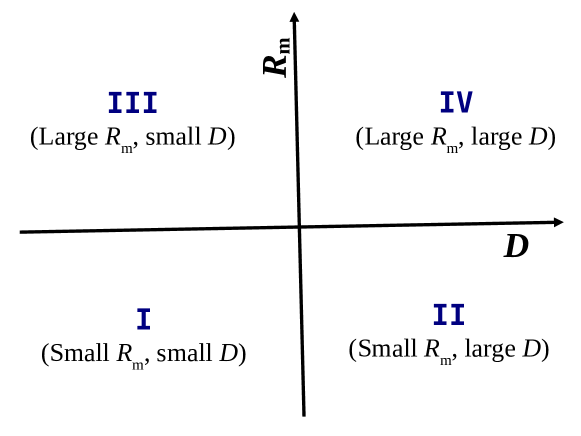
We perform a set of simulations in four different regimes in the parameter space $(R_{\rm m},D)$. We define the Regimes I, II, III, and IV as marked in Figure 1.

Figure 1.— Different regimes in magnetic Reynolds and dynamo numbers space to be studied in the present work.

3.1. Small $R_{\rm m}$ and small $D$: Regime I

In this regime, as both the Reynolds and the dynamo numbers are small, neither the small-scale dynamo nor the large-scale dynamo are possible. Therefore, any seed magnetic field decays with time. In Table 1, we show a typical run: R1 at $\nu=0.01$, $\eta=0.008$, $\sigma=1$ (fully helical forcing of positive helicity), and $S=-0.05$, so $R_{\rm m}=0.55$ and $D=4.1$, resulting in a slow decay at a rate $0.03u_{\rm rms}k_{1}$.

3.2. Small $R_{\rm m}$ and large $D$: Regime II

Next, we consider a set of parameters in Regime II. Run R2a is a typical simulation in this regime which is summarized in Table 1. In the two top panels of Figure 2, we show the $x$- and $y$-components of the mean field, $\overline{B}_{x}$ and $\overline{B}_{y}$. We see that the large-scale field is oscillatory with dynamo waves propagating in the positive $z$ direction. This is indeed expected because we force the flow with positive helicity, which results in a negative $\alpha$ effect, and since shear is also negative, the dynamo number is positive, resulting in dynamo wave propagation in the positive $z$ direction (see, e.g., Brandenburg & Subramanian, 2005). The toroidal field ($\overline{B}_{y}$, streamwise direction) is about 10 times stronger than the poloidal field ($\overline{B}_{x}$, cross-stream direction); see Figure 2. This is because of the fact that the $\Omega$ effect, as measured by $C_{\Omega}$, is much larger than the $\alpha$ effect, as measured by $C_{\alpha}$; see Table 1.

Figure 2.— Results from Run R2a in Regime II: Butterfly diagrams of $\overline{B}_{x}$, $\overline{B}_{y}$, $\overline{\bm{B}}^{2}$, and $\overline{\bm{b}^{2}}$ as functions of $z$ and $t$, normalized by the diffusive time scale $\tau_{\rm diff}=(k_{1}^{2}\eta)^{-1}$ ($k_{1}$ being the smallest possible wavenumber in the box). The field is always normalized by $B_{\rm eq}$. The initial phase for $t/\tau_{\rm diff}<30$ is not shown, because the magnetic field is still too weak.

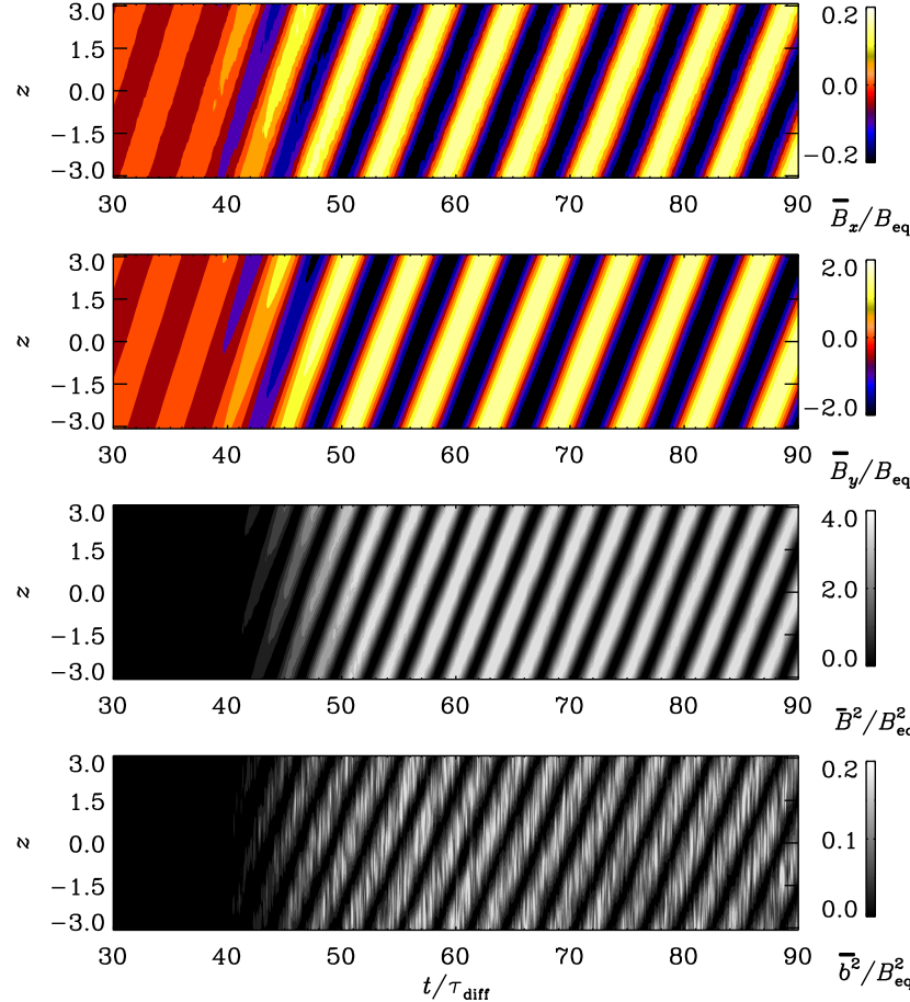
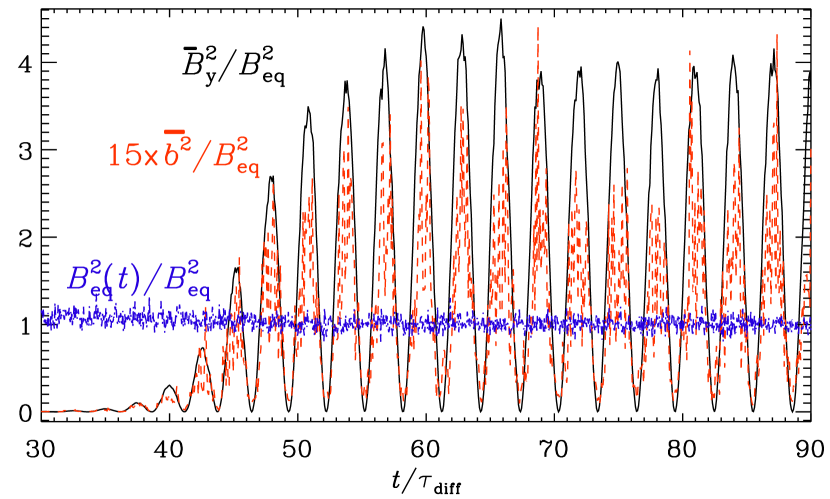
The next panel of Figure 2 shows the energy density of the large-scale field, $\overline{\bm{B}}^{2}$, and the last panel that of the small-scale field, $\overline{\bm{b}^{2}}$, as computed from Equation (7). An interesting feature to note is that the small-scale field is spatially and temporally correlated with the large-scale one. We also see that $\overline{\bm{b}^{2}}$ is much smaller than $\overline{\bm{B}}^{2}$. The time series of $\overline{B}_{y}^{2}$ and $\overline{\bm{b}^{2}}$ shown in Figure 3 show a tight correlation. Moreover, the small-scale field becomes significant only when the large-scale field does. In the early phase, this small-scale field grows linearly in time, contrary to the exponential growth when the field is generated through the small-scale dynamo.

A scatter plot between $\overline{B}_{y}^{2}$ and $\overline{\bm{b}^{2}}$ for all $z$ values shows a clear positive correlation with $\overline{\bm{b}^{2}}\approx q\overline{B}_{y}^{2}$; see Figure 4. It is interesting to compare this with results from the second order correlation approximation, which yields $q\approx R_{\rm m}^{2}$ when $R_{\rm m}\ll 1$ and the field is sufficiently weak; see Sect. 3.11 of Krause & Rädler (1980). However, here we find $q\sim 0.03$, which is about one order of magnitude smaller than $R_{\rm m}^{2}$ ($\sim 0.3$). One reason may well be that here the large-scale field is not imposed, as assumed in the analytic theory, but is the result of the large-scale dynamo.

Figure 3.— Results from Run R2a: Time series of $\overline{B}_{y}^{2}/B_{\rm eq}^{2}$ (solid black line), $\overline{\bm{b}^{2}}/B_{\rm eq}^{2}$ (red dashed), and $B_{\rm eq}^{2}(t)/B_{\rm eq}^{2}$ (blue dash-dotted). Note that $\overline{\bm{b}^{2}}/B_{\rm eq}^{2}$ is rescaled by a factor of 15.

Figure 4.— Results from R2a: Scatter plot between $\overline{B}_{y}^{2}/B_{\rm eq}^{2}$ and $\overline{\bm{b}^{2}}/B_{\rm eq}^{2}$ at $t/\tau_{\rm diff}>40$ (nonlinear phase) for all $z$. The inset displays the same variation, but in linear scale. The linear correlation coefficient $r$ between these two energies is $0.77$.

Our results demonstrate that in the present regime of small $R_{\rm m}$, the small-scale field is the result of tangling of the large-scale field and it is not due to the small-scale dynamo. We recall that the small-scale field developed in the global convection simulation of Racine et al. (2011) in spherical geometry also shows a positive correlation with the cyclic large-scale magnetic field. This suggests that the small-scale field in their simulation is also the result of tangling of the large-scale field rather than the local dynamo.

Figure 5.— Same as Figure 4, but from Run R2c. The red dashed line shows Equation (8)—the theoretical variation.

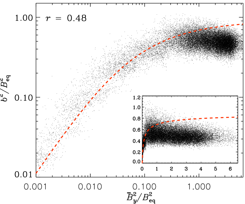
We have performed additional simulations in this regime by changing the parameters ($k_{\rm f}$, $\nu$, $\eta$, or $S$); see Runs R2b–R2h in Table 1. We notice that in Runs R2a, R2b and R2c, the large-scale magnetic field ($\tilde{\overline{B}}$) has not changed much as $D$ is similar in these runs, but $R_{\rm m}$ and the small-scale field ($\tilde{\overline{b}}$) have changed largely. The increase of $R_{\rm m}$ in these runs increases the tangling. Therefore, the small-scale magnetic field increases with increasing $R_{\rm m}$. Another interesting result we notice is that, unlike in the previous case at small $R_{\rm m}$ (Figure 4), tangling does not increase all the way with the large-scale field. To demonstrate this we show a scatter plot between $\overline{B}_{y}^{2}$ and $\overline{\bm{b}^{2}}$ for Run R2c—the case with the strongest $R_{\rm m}$ in Figure 5. Here we clearly observe the saturation of small-scale field. We also notice that when $\overline{B}_{y}^{2}$ just exceeds $B_{\rm eq}^{2}$ there is a small decrease of $\overline{\bm{b}^{2}}$—this is caused by the fact that, at this field strength, the flow is significantly suppressed which reduces the tangling. Then for $\overline{B}_{y}^{2}>B_{\rm eq}^{2}$, $\overline{\bm{b}^{2}}$ remains roughly constant.

The magnetic fluctuations produced in our simulations can be compared with the analytical theory of Rogachevskii & Kleeorin (2007) who have studied the magnetic fluctuations generated by tangling of the mean magnetic field through velocity fluctuations. Although in our simulations the values of $R_{\rm m}$ are rather small, we may try to compare with their analytical expression:

$$\overline{\bm{b}^{2}}=\overline{\bm{b}^{2}}^{(0)}+c_{1}\left(B_{\rm eq}^{2\,(0)}-\overline{\bm{b}^{2}}^{(0)}\right)f(c_{2}\beta),$$ (8)

with coefficients $c_{1}=1/12$, $c_{2}=4$, and $\beta=\overline{B}_{y}/B_{\rm eq}$, as well as the quenching function $f(\beta)=6-3A_{1}^{(0)}(\beta)-A_{2}^{(0)}(\beta)$ where $A_{1}^{(0)}(\beta)$ and $A_{2}^{(0)}(\beta)$ are given by

$$A_{1}^{(0)}(\beta)=\frac{1}{5}\left[2+2\frac{\tan^{-1}\beta}{\beta^{3}}\right](3+5\beta^{2})-\frac{6}{\beta^{2}}$$

$$-\beta^{2}\ln R_{\rm m}-2\beta^{2}\ln\left(\frac{1+\beta^{2}}{1+\beta^{2}\sqrt{R_{\rm m}}}\right),$$

$$A_{2}^{(0)}(\beta)=\frac{2}{5}\left[2-\frac{\tan^{-1}\beta}{\beta^{3}}\right](9+5\beta^{2})+\frac{9}{\beta^{2}}$$

$$-\beta^{2}\ln R_{\rm m}-2\beta^{2}\ln\left(\frac{1+\beta^{2}}{1+\beta^{2}\sqrt{R_{\rm m}}}\right).$$ (9)

The above Equation (8) is obtained by ignoring the effects of convection, which corresponds to putting the parameter $a_{*}=0$ in Eq. (A21) of Rogachevskii & Kleeorin (2007). The superscripts $(0)$ indicate that these values are not affected by the mean magnetic field, so they are the kinematic values, hence $B_{\rm eq}^{2\,(0)}$ is the unquenched value of $\mbox{\boldmath$u$}{}^{2}$ and $\overline{\bm{b}^{2}}^{(0)}$ is the contribution from the small-scale dynamo, which is equal to zero as in this case there is no small-scale dynamo. We compute $\overline{\bm{b}^{2}}$ from Equation (8) and display it as a dashed line in Figure 5. We see that the analytical theory, which is valid for $R_{\rm m}\gg 1$ and $\mbox{\rm Re}\gg 1$, is not far from our simulation data, which are at much smaller $R_{\rm m}$ ($\approx 20$) and Re ($\approx 40$). Our result generally confirms the theoretical prediction of the saturation of small-scale magnetic field at $\overline{B}_{y}>B_{\rm eq}$.

Returning to the other runs in this regime (R2d–R2h), we notice that $R_{\rm m}$ is not much different in these runs, but the values of $D$ have increased systematically from Run R2d to Run R2h. The small-scale field ($\tilde{\overline{b}}$) has also increased systematically in these runs. This clearly demonstrates that the tangling increases not only with $R_{\rm m}$, but also with the large-scale field itself. However, in all these runs, except in Run R2d, we again observe the saturation of small-scale field for $\overline{B}_{y}>B_{\rm eq}$.

3.3. Large $R_{\rm m}$ and vanishing $D$: Regime III

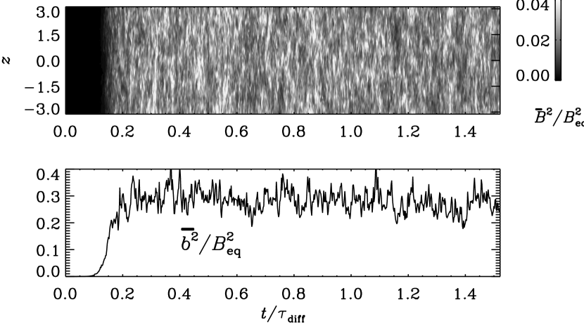
We perform a simulation with $\sigma=0$ (non-helical), and $S=0$. Run R3 in Table 1 represents this simulation. When $C_{\alpha}=0$ and $C_{\Omega}=0$, we should not expect a large-scale magnetic field to develop. We have chosen such setup to exclude the effect of the large-scale magnetic field in this simulation. The top panel of Figure 6 shows the energy of the large-scale field $\overline{\bm{B}}^{2}$. We do not see any large-scale structures comparable to the system size. In any case, the small-scale dynamo is expected to be excited as in this case the magnetic Reynolds number $R_{\rm m}\sim 86$ is sufficiently large for large values of the magnetic Prandtl number, $P_{\rm m}=5$, to excite the small-scale dynamo. This is indeed confirmed by the present results.

In the bottom panel of Figure 6, we show the time series of the energy density of the small-scale field. Initially this field grows exponentially in time and then remains constant. The characteristic length scale of this field is, as expected for a small-scale dynamo, smaller than the forcing scale of the turbulence, as can be seen from the magnetic energy spectrum in Figure 8 (thick dashed curve).

Figure 6.— Results from Run R3 in Regime III: Butterfly diagram of the energy density of the large-scale magnetic field $\overline{\bm{B}}^{2}$ (top) and time series of the small-scale field $\overline{\bm{b}^{2}}$ at $z=0$ (bottom).

3.4. Large $R_{\rm m}$ and large $D$: Regime IV

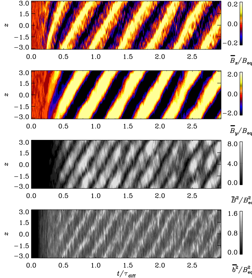
Our first two models in Regime IV are similar to Run R3, but with finite shear and helicity such that the large-scale dynamo is excited. We begin with $S=-0.05$ and $\sigma=1$. In Table 1, we refer to this run as R4a. The magnetic butterfly diagrams of various quantities are displayed in Figure 7. Again, we see dynamo waves of the large-scale field components propagating in the positive $z$ direction. The mean toroidal field ($\overline{B}_{y}$) is here about 10 times stronger than the mean poloidal field ($\overline{B}_{x}$).

Figure 7.— Results from Run R4a in Regime IV: Butterfly diagrams of $\overline{B}_{x}$, $\overline{B}_{y}$, $\overline{\bm{B}}^{2}$, and $\overline{\bm{b}^{2}}$.

Figure 8.— Evolutions of the energy spectra $E_{K}(k,t)$ (thin curves) and $E_{M}(k,t)$ (thick) for Run R3^′ (SSD, dashed curves) and Run R4a^′ (SSD+LSD, solid and dotted lines correspond to magnetic maxima and minima, respectively). All spectra are temporally averaged excluding the initial growing phase.

Figure 9.— Results from Run R4a: Time series of $\overline{B}_{y}^{2}$ (solid black line), $\overline{\bm{b}^{2}}$ (red dashed), and $B_{\rm eq}^{2}(t)$ (blue dash-dotted). Note that $\overline{\bm{b}^{2}}/B_{\rm eq}^{2}$ is rescaled by a factor of two.

Figure 10.— Results from Run R4a: A scatter plot between $\overline{B}_{y}^{2}/B_{\rm eq}^{2}$, and $\overline{\bm{b}^{2}}/B_{\rm eq}^{2}$ at different values of $z$ coordinate. The red dashed line shows the $\overline{\bm{b}^{2}}\propto\overline{B}_{y}^{-1.4}$ dependence, whereas blue dotted line represents Equation (8). The data points for initial growth phase ($t/\tau_{\rm diff}<0.6$) are not used for this plot. The linear correlation coefficient $r$ is marked on the plot.

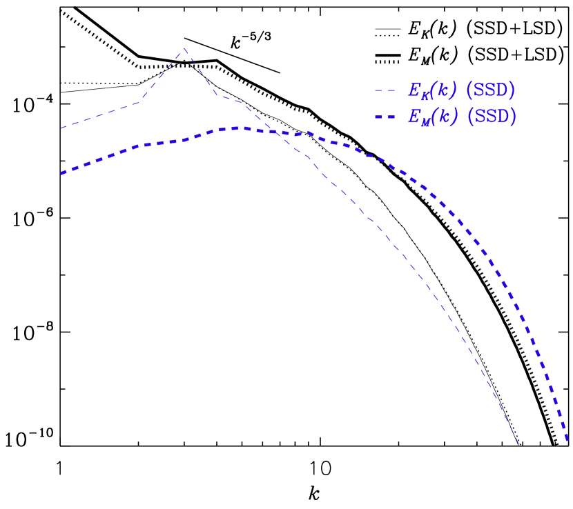
In Figure 8, we show for Run R4a^′ (a high resolution version of Run R4a) kinetic and magnetic energy spectra, $E_{K}(k,t)$ (thin solid and dotted) and $E_{M}(k,t)$ (thick solid and dotted), during magnetic maximum and minimum, respectively. For comparison we also show the spectra for a small-scale dynamo from Run R3^′ (a high resolution version of Run R3). For both dynamos, $E_{K}(k,t)$ has a peak at the forcing wavenumber which is around 3 in these cases, followed by a small inertial range, that is slightly steeper than $k^{-5/3}$, and finally the energy dissipation at small scales. However, $E_{M}(k,t)$ shows different behaviors in the two cases. For the LSD there is an intermediate peak slightly below the forcing scale ($k\approx 4$) and then there is a maximum at the largest scale ($k=1$), as expected for the large-scale dynamo. During magnetic maximum, $E_{M}(k,t)$ is larger at large scales (compare thick solid and dotted curves), but it is slightly smaller at small scales ($k>20$). However, during magnetic maximum $E_{K}(k,t)$ is slightly smaller at larger scale ($k<3$; compare thin solid and dotted curves).

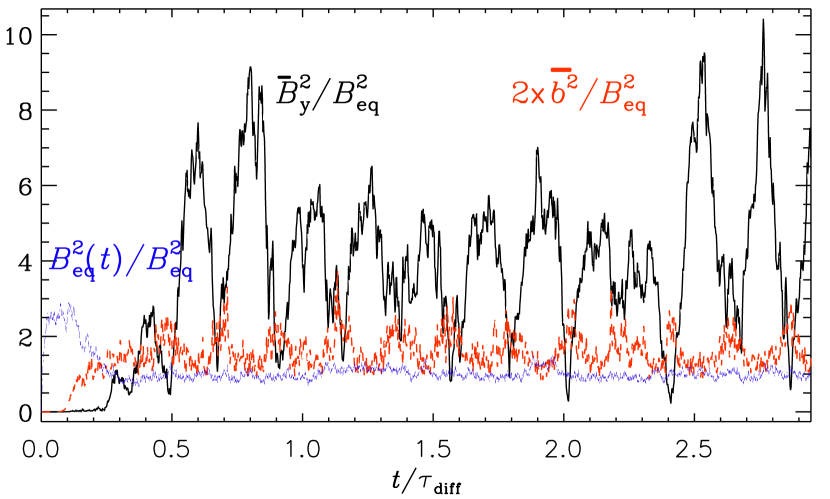
Owing to the cyclic variation of the large-scale field we see a weak modulation of the energy of the small-scale field, as seen in the lower two panels of Figure 7. In fact, $\overline{\bm{b}^{2}}$ shows a weak anticorrelation with $\overline{\bm{B}^{2}}$. This is evident from Figure 9, where time series of $\overline{B}_{y}^{2}$ and $\overline{\bm{b}^{2}}$ at $z=0$ are shown. From Figure 9 we note that $\overline{\bm{b}^{2}}$ reaches significant levels much faster than the large-scale energy. This implies that initially $\overline{\bm{b}^{2}}$ is primarily a result of the small-scale dynamo, which grows faster than the large-scale dynamo. Later, with the development of the large-scale field, $\overline{\bm{b}^{2}}$ increases further. Eventually, in this run, the saturated value of $\overline{\bm{b}^{2}}$ is much larger than that in Run R3 (which is basically the same as in this run, but only the small-scale dynamo is excited because of taking $\sigma=0$, and $S=0$; see Table 1).

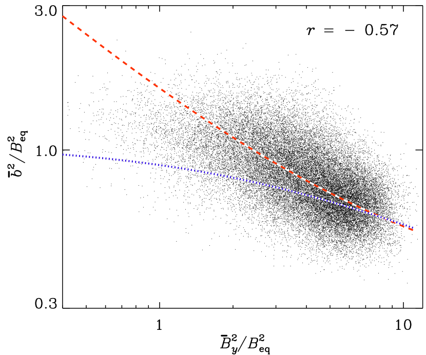
Considering only the nonlinear stage ($\overline{B}_{y}\geq B_{\rm eq}$), we produce in Figure 10 a scatter plot between $\overline{B}_{y}^{2}$ and $\overline{\bm{b}^{2}}$ for all grid points along the $z$ direction. This shows an anticorrelation obeying $\overline{\bm{b}^{2}}\propto\overline{B}_{y}^{\,-1.4}$; see the red dashed line. The linear correlation coefficient between $\overline{B}_{y}^{2}$ and $\overline{\bm{b}^{2}}$ is $-0.57$. It is not straightforward to understand the origin of such variations: the small-scale magnetic field developed in this simulation can be read as $\overline{\bm{b}^{2}}=\overline{\bm{b}^{2}}_{\rm SSD}+\overline{\bm{b}^{2}}_{\rm tang}$, where $\overline{\bm{b}^{2}}_{\rm SSD}$ results purely from the small-scale dynamo, while $\overline{\bm{b}^{2}}_{\rm tang}$ results from the tangling of the large-scale field. Unfortunately, separating these two quantities from a given simulation is not an easy task because both quantities are affected by the large-scale field $\overline{\mbox{\boldmath$B$}}{}$. In the initial phase, when the large-scale field is not yet fully developed, the small-scale field is mainly a consequence of the small-scale dynamo. Thus, in this phase we have $\overline{\bm{b}^{2}}\approx\overline{\bm{b}^{2}}_{\rm SSD}$. Then, with increasing $\overline{\mbox{\boldmath$B$}}{}^{2}$, the small-scale field is increasing further because of the contribution from the tangling of the large-scale field. However, when $\overline{\mbox{\boldmath$B$}}{}^{2}$ exceeds $B_{\rm eq}^{2}$, $\overline{\bm{b}^{2}}_{\rm tang}$ tends to saturate. (Such behavior was seen in earlier simulations of Section 3.2 showing that, when the small-scale dynamo was not operating, the small-scale field generated due to tangling of the large-scale field increased with the mean-field first and then saturated; see Figure 5.) Therefore, in the nonlinear phase of the present simulation, the anticorrelation results from the fact that the small-scale dynamo is suppressed by the large-scale magnetic field through the Lorentz force acting on the flow. However, when we look at the energy of the turbulence, $B_{\rm eq}^{2}(t)$ ($=\mbox{\boldmath$u$}{}^{2}$), as shown in Figure 9, we see no anticorrelation between the flow and the large-scale field. This is possibly because our turbulence is continuously forced by a forcing function which could break the anticorrelation between $\overline{B}_{y}^{2}$ and $\mbox{\boldmath$u$}{}^{2}$.

Keeping in mind that the theory of Rogachevskii & Kleeorin (2007) was developed for magnetic fluctuations generated due to tangling and a small-scale dynamo represented by a constant factor $\overline{\bm{b}^{2}}^{(0)}$, which is not the case here, we now try to fit our data by choosing different values of $p$ and $q$ in Equation (8). We find that, when $\overline{\bm{b}^{2}}^{(0)}=1.02B_{\rm eq}^{2\,(0)}$, $c_{1}=4.0$, and $c_{2}=0.5$, there is moderate agreement, but only for $2<\overline{B}_{y}^{2}/B_{\rm eq}^{2}<10$; see blue dotted line in Figure 10.

Figure 11.— Same as Figure 9 but results from R4g.

Figure 12.— Same as Figure 10 but results from Run R4g. The data points for initial growth phase ($t/\tau_{\rm diff}<0.3$) are not used for this plot.

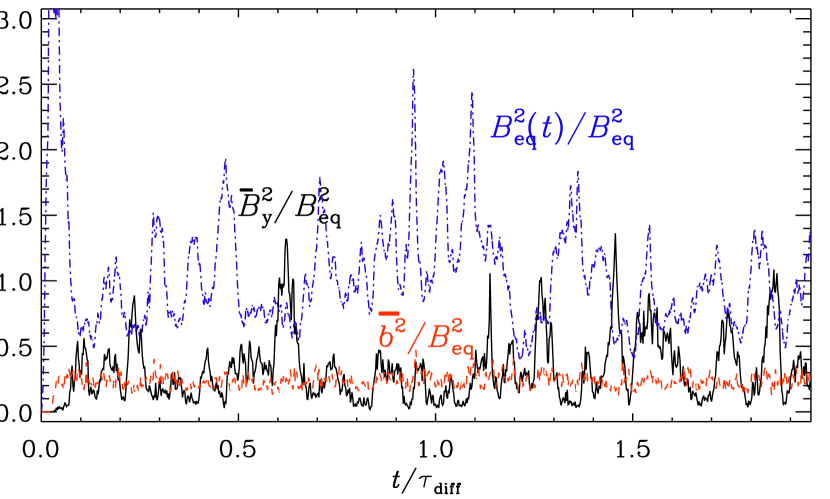
We have performed a few more simulations in this regime (see Runs R4b–R4h in Table 1) at different values of $R_{\rm m}$, $P_{\rm m}$, or $D$. We observe that, as long as the large-scale field is above $B_{\rm eq}$, the small-scale field is anticorrelated with the large-scale field. This is the case for Runs R4a–R4f. However for Runs R4g and R4h we see that the large-scale dynamo is much weaker (compare the $D$ values) and consequently the large-scale field is much weaker than $B_{\rm eq}$ so that it cannot affect the small-scale field production significantly. Therefore, we do not see any anticorrelation between small- and large-scale fields in this case. In Figure 11 we show the time series of $\overline{B}_{y}^{2}$ and $\overline{\bm{b}^{2}}$ and in Figure 12 the corresponding scatter plot for Run R4g. Here we do not see any anticorrelation between the small-scale and the large-scale fields. Another feature to note is that in the earlier Runs R4a–R4f the small-scale field $\tilde{\overline{b}}$ was more than $82\%$ of $B_{\rm eq}$ (see Table 1), whereas in Runs R4g–R4h the small-scale field is only about $48\%$ of $B_{\rm eq}$. We would expect the opposite because the small-scale dynamo should be much stronger as $R_{\rm m}$ is larger in the latter two runs. Therefore, larger values of $\tilde{\overline{b}}$ in Runs R4a–R4f compared to Runs R4g–R4h imply that a significant contribution of small-scale field in Runs R4a–R4f is coming from tangling.

On this occasion we mention that, using the same setup as here, Hubbard et al. (2011) have demonstrated that, after some initial saturation phase, the $\alpha\Omega$ dynamo mode is “fratricided” by a separate $\alpha^{2}$ mode and eventually the initial $\alpha\Omega$ model changes to an $\alpha^{2}$ type dynamo, which is sustained by the helical turbulence alone. Some of the simulations, particularly at larger $R_{\rm m}$ and large $D$ (Runs R4a–R4f), display such behavior. Therefore, analyzing these simulations for longer durations is problematic. In this connection it maybe useful to note that the typical wall clock time per timestep per mesh point for simulations with $144^{3}$ meshpoints using 48 processors is about $0.07~{}\mu$s. Therefore, for example, to produce results for Run R4a (presented in Figure 7) it took about 24 hours, while for R4g (Figure 11) it took 43 hours. As examples, for Runs R2a and R4g, $\tau_{\rm diff}/\Delta t\approx$ 2400 and 410000, respectively.

4. Summary and conclusions

We have performed a set of simulations in different parameter regimes of Reynolds and dynamo numbers to explore the effect of the cyclic variation of the dynamo-generated large-scale magnetic field on the small-scale field. Our ultimate motivation is to shed some light on the solar cycle dependence of the small-scale magnetic field at the solar surface. In the Sun, both global and local dynamos are expected to operate at the same time and can in principle occur even in the same location. To study this problem in detail, it is necessary to develop a model in which both dynamos are operating. We have therefore considered a simple turbulent dynamo in which the fluid is helically forced and large-scale linear shear is imposed. This simple setup captures the essential mechanism of an $\alpha\Omega$ dynamo believed to be operating in the Sun. At the same time, the local dynamo can be excited in this setup when $R_{\rm m}$ exceeds a critical value. The main advantage of considering this type of simple setup, rather than considering more sophisticated global convection simulations in spherical geometry (Hotta et al., private communication) are an affordable computational expense and that we can easily change the large-scale dynamo parameters to explore different regimes of these two dynamos.

In Regime III, when the large-scale dynamo number is small but the Reynolds number is large, we observe only the small-scale dynamo in which the generated small-scale field does not have any temporal variation. This situation does not apply to the Sun as large-scale magnetic field is also generating by the global dynamo. In Regime IV (Section 3.4), when both the Reynolds and dynamo numbers are large, we observe both dynamos—the large-scale dynamo producing an oscillatory large-scale magnetic field and the local dynamo producing a small-scale field. This situation is relevant to the Sun. In our simulations, we observe that the small-scale field is almost uncorrelated with the dynamo cycle as long as the large-scale field is smaller than the equipartition value of turbulence. However, when the large-scale field is stronger than the equipartition value, we observe that the generation of the small-scale field is quenched by the large-scale field—producing a weak anticorrelation between small- and large-scale fields. This reciprocal correlation between the small-scale field and the global dynamo cycle is in agreement with observations of the small-scale magnetic field at the solar surface (e.g., Hagenaar et al., 2003; Jin et al., 2011; Jin & Wang, 2012, 2015a; Faurobert & Ricort, 2015). In particular, Jin et al. (2011) have analyzed separately the small-scale elements based on their magnetic flux contents and the number of magnetic elements and found that their cyclic variations for magnetic elements with fluxes in the range $\sim(3$–$30)\times 10^{18}\,{\rm Mx}$ and $\sim(4$–$40)\times 10^{19}\,{\rm Mx}$ show anticorrelation and correlation with sunspots, respectively. Further analysis by Jin & Wang (2012) has revealed that this anticorrelated component shows a solar cycle variation different from the sunspot variation in time and latitude, whereas the correlated component shows similarities with the sunspot butterfly diagram. Based on our simulation results in Regime IV, and the observational results, we conclude that the small-scale magnetic field observed at the solar surface (particularly, the magnetic elements with fluxes $\leq 3\times 10^{19}\,{\rm Mx}$ in the analysis of Jin et al., 2011) are a consequence of both the small-scale dynamo generated locally in the solar convection zone and the shredding and tangling of the large-scale magnetic field generated by the global dynamo. On the other hand, the magnetic field with a flux above $4\times 10^{19}\,{\rm Mx}$, but smaller than the active region flux in the analysis of Jin et al. (2011), are possibly the result of shredding and tangling of the large-scale magnetic field generated by the global dynamo only. Our simulations in Regime II (Section 3.2), when the dynamo number is large but the Reynolds number is small, illustrate this situation because in this case the local dynamo is not possible and the small-scale field is still generated by the tangling of the large-scale magnetic field.

We reiterate that we observe a weak anti-correlation between small-scale field and large-scale magnetic cycle only when the large-scale field is much stronger than the equipartition value. Based on our knowledge, we can say that the large-scale field in the solar convection zone may be larger than the equipartition value, although probably not by much. Therefore we expect that the small-scale magnetic field in the Sun is largely unaffected by the global large-scale cycle, but not completely. The lack or weakness of a variation of the small-scale magnetic field observed in our simple turbulent dynamo simulations certainly support the idea that both the small-scale dynamo and the tangling of large-scale field are responsible for the observed small-scale magnetic field in the Sun. In fact, in certain regimes our results are in agreement with observations of the small-scale magnetic field. However, future studies using more realistic solar dynamo models will be useful for more quantitative comparisons.

References

- Batchelor (1950) Batchelor, G. K. 1950, Roy. Soc. Lond. Proc. Ser. A, 201, 405
- Blackman & Brandenburg (2002) Blackman, E. G., & Brandenburg, A. 2002, ApJ, 579, 359
- Boldyrev & Cattaneo (2004) Boldyrev, S., & Cattaneo, F. 2004, Phys. Rev. Lett., 92, 144501
- Brandenburg (1998) Brandenburg, A. 1998, in Astron. Soc. Pac. Conf. Ser., Vol. 154, Cool Stars, Stellar Systems, and the Sun, ed. R. A. Donahue & J. A. Bookbinder, 173
- Brandenburg (2005) Brandenburg, A. 2005, ApJ, 625, 539
- Brandenburg (2011) —. 2011, ApJ, 741, 92
- Brandenburg et al. (2011) Brandenburg, A., Kemel, K., Kleeorin, N., Mitra, D., & Rogachevskii, I. 2011, ApJ, 740, L50
- Brandenburg et al. (2013) Brandenburg, A., Kleeorin, N., & Rogachevskii, I. 2013, ApJ, 776, L23
- Brandenburg & Subramanian (2005) Brandenburg, A., & Subramanian, K. 2005, Phys. Rep., 417, 1
- Buehler et al. (2013) Buehler, D., Lagg, A., & Solanki, S. K. 2013, A&A, 555, A33
- Cattaneo (1999) Cattaneo, F. 1999, ApJ, 515, L39
- Charbonneau (2014) Charbonneau, P. 2014, Ann. Rev. Astron. Astrophys., 52, 251
- Childress & Gilbert (1995) Childress, S., & Gilbert, A. D. 1995, Stretch, Twist, Fold (Springer-Verlag Berlin Heidelberg New York)
- Choudhuri et al. (1995) Choudhuri, A. R., Schüssler, M., & Dikpati, M. 1995, A&A, 303, L29
- de Wijn et al. (2005) de Wijn, A. G., Rutten, R. J., Haverkamp, E. M. W. P., & Sütterlin, P. 2005, A&A, 441, 1183
- de Wijn et al. (2009) de Wijn, A. G., Stenflo, J. O., Solanki, S. K., & Tsuneta, S. 2009, Space Sci. Rev., 144, 275
- Durney et al. (1993) Durney, B. R., De Young, D. S., & Roxburgh, I. W. 1993, Sol. Phys., 145, 207
- Emonet & Cattaneo (2001) Emonet, T., & Cattaneo, F. 2001, ApJ, 560, L197
- Faurobert & Ricort (2015) Faurobert, M., & Ricort, G. 2015, A&A, in press
- Frazier & Stenflo (1972) Frazier, E. N., & Stenflo, J. O. 1972, Sol. Phys., 27, 330
- Gošić et al. (2014) Gošić, M., Bellot Rubio, L. R., Orozco Suárez, D., Katsukawa, Y., & del Toro Iniesta, J. C. 2014, ApJ, 797, 49
- Hagenaar et al. (2003) Hagenaar, H. J., Schrijver, C. J., & Title, A. M. 2003, ApJ, 584, 1107
- Haugen et al. (2004) Haugen, N. E., Brandenburg, A., & Dobler, W. 2004, Phys. Rev. E, 70, 016308
- Hazra et al. (2014) Hazra, G., Karak, B. B., & Choudhuri, A. R. 2014, ApJ, 782, 93
- Hotta et al. (2014) Hotta, H., Rempel, M., & Yokoyama, T. 2014, ApJ, 786, 24
- Hotta et al. (2015) —. 2015, ApJ, 803, 42
- Howard & Stenflo (1972) Howard, R., & Stenflo, J. O. 1972, Sol. Phys., 22, 402
- Hubbard et al. (2011) Hubbard, A., Rheinhardt, M., & Brandenburg, A. 2011, A&A, 535, A48
- Iskakov et al. (2007) Iskakov, A. B., Schekochihin, A. A., Cowley, S. C., McWilliams, J. C., & Proctor, M. R. E. 2007, Phys. Rev. Lett., 98, 208501
- Jin & Wang (2015a) Jin, C., & Wang, J. 2015a, ApJ, 806, 174
- Jin & Wang (2012) Jin, C. L., & Wang, J. X. 2012, ApJ, 745, 39
- Jin & Wang (2015b) —. 2015b, ApJ, 807, 70
- Jin et al. (2011) Jin, C. L., Wang, J. X., Song, Q., & Zhao, H. 2011, ApJ, 731, 37
- Käpylä & Brandenburg (2009) Käpylä, P. J., & Brandenburg, A. 2009, ApJ, 699, 1059
- Käpylä et al. (2013) Käpylä, P. J., Mantere, M. J., Cole, E., Warnecke, J., & Brandenburg, A. 2013, ApJ, 778, 41
- Karak et al. (2014) Karak, B. B., Jiang, J., Miesch, M. S., Charbonneau, P., & Choudhuri, A. R. 2014, Space Sci. Rev., 186, 561
- Karak et al. (2015a) Karak, B. B., Käpylä, P. J., Käpylä, M. J., Brandenburg, A., Olspert, N., & Pelt, J. 2015a, A&A, 576, A26
- Karak et al. (2015b) Karak, B. B., Kitchatinov, L. L., & Brandenburg, A. 2015b, ApJ, 803, 95
- Kazantsev (1968) Kazantsev, A. P. 1968, Sov. J. Exp. Theor. Phys., 26, 1031
- Kemel et al. (2013) Kemel, K., Brandenburg, A., Kleeorin, N., Mitra, D., & Rogachevskii, I. 2013, Sol. Phys., 287, 293
- Krause & Rädler (1980) Krause, F., & Rädler, K. H. 1980, Mean-field magnetohydrodynamics and dynamo theory (Oxford: Pergamon Press)
- Lites (2011) Lites, B. W. 2011, ApJ, 737, 52
- Lites et al. (2008) Lites, B. W., et al. 2008, ApJ, 672, 1237
- McClintock et al. (2014) McClintock, B. H., Norton, A. A., & Li, J. 2014, ApJ, 797, 130
- Petrovay & Szakaly (1993) Petrovay, K., & Szakaly, G. 1993, A&A, 274, 543
- Pietarila Graham et al. (2010) Pietarila Graham, J., Cameron, R., & Schüssler, M. 2010, ApJ, 714, 1606
- Racine et al. (2011) Racine, É., Charbonneau, P., Ghizaru, M., Bouchat, A., & Smolarkiewicz, P. K. 2011, ApJ, 735, 46
- Rempel (2014) Rempel, M. 2014, ApJ, 789, 132
- Rogachevskii & Kleeorin (1997) Rogachevskii, I., & Kleeorin, N. 1997, Phys. Rev. E, 56, 417
- Rogachevskii & Kleeorin (2007) —. 2007, Phys. Rev. E, 76, 056307
- Sánchez Almeida (2003) Sánchez Almeida, J. 2003, A&A, 411, 615
- Schekochihin et al. (2005) Schekochihin, A. A., Haugen, N. E. L., Brandenburg, A., Cowley, S. C., Maron, J. L., & McWilliams, J. C. 2005, ApJ, 625, L115
- Schrijver & Harvey (1994) Schrijver, C. J., & Harvey, K. L. 1994, Sol. Phys., 150, 1
- Schrijver et al. (1998) Schrijver, C. J., et al. 1998, Nature, 394, 152
- Sokoloff et al. (2015) Sokoloff, D., Khlystova, A., & Abramenko, V. 2015, MNRAS, 451, 1522
- Spruit et al. (1987) Spruit, H. C., Title, A. M., & van Ballegooijen, A. A. 1987, Sol. Phys., 110, 115
- Stenflo (2012) Stenflo, J. O. 2012, A&A, 547, A93
- Tobias et al. (2011) Tobias, S. M., Cattaneo, F., & Brummell, N. H. 2011, ApJ, 728, 153
- Vögler & Schüssler (2007) Vögler, A., & Schüssler, M. 2007, A&A, 465, L43
- Vögler et al. (2005) Vögler, A., Shelyag, S., Schüssler, M., Cattaneo, F., Emonet, T., & Linde, T. 2005, A&A, 429, 335
- Zhou et al. (2013) Zhou, G., Wang, J., & Jin, C. 2013, Sol. Phys., 283, 273