The Charmonium Potential at Non-Zero Temperature

Abstract

The potential between charm and anti-charm quarks is calculated non-perturb-atively using physical, rather than static quarks at temperatures on both sides of the deconfinement transition $T_{\rm C}$, using a lattice simulation with 2+1 dynamical quark flavours. We used the hal qcd time-dependent method, originally developed for inter-nucleon potentials. Our lattices are anisotropic, with temporal lattice spacing less than the spatial one which enhances the information content of our correlators at each temperature. Local-extended charmonium correlators were calculated efficiently by contracting propagators in momentum rather than coordinate space. We find no significant variation in the central potential for temperatures in the confined phase. As the temperature increases into the deconfinement phase, the potential flattens, consistent with the expected weakening interaction. We fit the potential to both the (a) Cornell and (b) Debye-screened potential forms, with the latter better reproducing the data. The zero temperature string tension obtained from (a) agrees with results obtained elsewhere, and it decreases with temperature, but at a slower rate than from the static quark approximation. The Debye mass from (b) is close to zero for small temperatures, but starts to increase rapidly around $T_{\rm C}$. The spin-dependent potential is found to have a repulsive core and a distinct temperature dependence above $T_{\rm C}$ at distances $\sim 1$ fm.

1 Introduction

Shortly after the discovery of the $J/\psi$ particle, it was realised that charmonium bound states could be very well described using the Schrödinger equation with a phenomenological potential between the quark and antiquark Eichten:1974af ; Eichten:1978tg ; Eichten:1979ms . This was one of the factors leading to QCD being accepted as the theory of the strong interaction, with charmonium as the ‘hydrogen atom’ of QCD. The validity of a potential model has since been formally established using an effective theory — potential nonrelativistic QCD (pNRQCD) — which is obtained by integrating out degrees of freedom with momentum above the typical binding energy of the system Brambilla:1999xf ; Brambilla:2004jw . The resulting potential for infinitely heavy (static) quarks can be shown to be equivalent to the one extracted from the Wilson loop, which has been computed non-perturbatively from first principles on the lattice. Recently, the potential between quarks with finite mass has also been computed from lattice QCD by ‘reverse engineering’ the Schrödinger equation Ikeda:2010nj ; Ikeda:2011bs ; Kawanai:2011xb ; Kawanai:2011jt ; Kawanai:2011fh ; Kawanai:2013aca using the hal qcd method Ishii:2006ec .

At non-zero temperature, a potential model incorporating colour-Debye screening has been used to predict the dissociation of charmonium states as a signal for the formation of quark-gluon plasma (QGP) Matsui:1986dk . Since that seminal paper, a substantial experimental effort has been invested in the study of $J/\psi$ suppression at SPS, RHIC and the LHC Abreu:2000ni ; Chatrchyan:2012np ; Adcox:2004mh ; Adams:2005dq , and a number of studies have been carried out using potential models for charmonium systems at high temperature Mocsy:2007yj ; Mocsy:2005qw ; Mocsy:2004bv . However, unlike at zero temperature, there was no rigorous proof of the validity of potential models for static quarks and hence no agreement on what to use for the interquark potential. Different groups have used, for example, the free energy Kaczmarek:2005ui ; Fodor:2007mi or the internal energy Kaczmarek:2005gi of static quarks as computed on the lattice, or a combination of these Wong:2004zr ; Wong:2005be .

Recently, a series of effective theories has been developed, depending on hierarchies such as

$$M_{q}\gg T>g^{2}M_{q}>gT\gg g^{4}M_{q}\quad\text{or}\quad M_{q}\gg g^{2}M_{q}>T\gg gT\gg g^{4}M_{q},$$ (1)

where $M_{q}$ is the heavy quark mass, $T$ is the temperature and $g$ is the gauge coupling. A common feature of these theories is the appearance of an imaginary part of the potential, resulting from Landau damping Laine:2006ns ; Laine:2007qy . In certain parameter ranges this term can be more important for charmonium suppression than the Debye screening encoded in the real part.

As in the zero temperature case, non-perturbative (lattice) calculations of the Wilson loop have been used to extract the static inter-quark potential at non-zero temperature Rothkopf:2011db ; Burnier:2012az ; Bazavov:2012bq ; Bazavov:2012fk .

In this work we further extend these non-perturbative lattice calculations to the finite quark mass case. We will assume the validity of the Schrödinger equation and potential description for charm quarks, and derive the charmonium potential at non-zero temperature directly from charmonium correlators following the hal qcd method. We restrict ourselves to the real part of the potential and will be following the ‘time-dependent’ method introduced in Aoki:2012tk . This method was used in Evans:2013yva but is distinct from the ‘fitting’ method used in Allton:2013wza . In the fitting method, local-extended correlators are first fitted to exponentials at large Euclidean time, $\tau$, to extract the Nambu-Bethe-Salpeter (NBS) ground state wave function. The NBS wave function is then used, in conjunction with the Schrödinger equation, to reverse-engineer the potential. The fitting method is well understood from a theoretical point of view since it relies on conventional fitting techniques. However, at non-zero temperature, where the temporal range of the correlators is limited, it suffers from familiar limitations: higher excited states still contribute to the correlator at the largest available $\tau$, making fits unreliable.

In Iida:2011za the first calculation of the charmonium potential at finite mass and non-zero temperature was performed, but this used the quenched approximation. We performed thermal studies of the charmonium potential using our two-flavour, 1st generation fastsum ensembles in our previous study Evans:2013yva ; Allton:2013wza . In the work presented here, we extend this by using our 2nd generation ensembles which have 2+1 flavours with finer, larger lattices and light quarks closer to their physical masses. We find that the potential does not vary significantly for temperatures below the crossover temperature, $T_{C}$, but that it clearly flattens above $T_{C}$. Using the Cornell form of the potential, we determine the temperature dependent string tension which decreases as $T$ increases as expected. We also fit our data to a Debye-screened potential form to determine the Debye mass. The spin-dependent potential is also determined and we find thermal effects for $T\;\raisebox{-2.15277pt}{\hbox to0.0pt{$\sim$\hss}}\raisebox{2.15277pt}{$>$}\;T_{C}$. An early version of this work appears in Evans:2013zca .

In section 2, the hal qcd time-dependent method is reviewed, and we discuss the effect of the backward moving states. Our simulation details are outlined in section 3 and section 4 presents our results.

2 The Method

Figure 1: Quark propagator diagram of a local-extended correlator. The quark and anti-quark are created at the source with no separation and annihilated at the sink with a separation $\mathbf{r}$.

The hal qcd time-dependent method of extracting the potential from the lattice Aoki:2012tk takes local-extended correlators as input, see Figure 1. These are constructed from creation and annihilation operators that have the form

$$J_{\Gamma}(x;\mathbf{r})=\bar{q}(x)\,\Gamma\,U(x,x\!+\!\mathbf{r})\,q(x\!+\!\mathbf{r}),$$ (2)

where $\mathbf{r}$ is the separation between the quark and anti-quark fields $q$ and $\bar{q}$, $x$ is the space-time point $(\mathbf{x},\tau)$ and $\Gamma$ is a monomial of gamma matrices used to generate pseudoscalar ($\eta_{c}$) channels or vector ($J/\psi$). $U(x,x\!+\!\mathbf{r})$ is the gauge connection between $x$ and $x+\mathbf{r}$ required for gauge invariance.

The local-extended charmonium correlator is

$$C_{\Gamma}(\mathbf{r},\tau)=\sum_{\mathbf{x}}\langle J_{\Gamma}(\mathbf{x},\tau;\mathbf{r})\;J_{\Gamma}^{\dagger}(0;\mathbf{0})\rangle,$$ (3)

where the sum over the spatial coordinate at the sink, $\mathbf{x}$, projects the momentum of the state to zero.

The local-extended correlator can also be expressed as a sum over the eigenstates of the Hamiltonian with eigenvalues $E_{j}$,

$$C_{\Gamma}(\mathbf{r},\tau)=\sum_{j}\frac{\psi_{j}^{\ast}(\mathbf{0})\psi_{j}(\mathbf{r})}{2E_{j}}\;\left(e^{-E_{j}\tau}+e^{-E_{j}(N_{\tau}-\tau)}\right),$$ (4)

where the sum is over the states $j$ with the same Lorentz transformation properties as the operator $J_{\Gamma}$, $N_{\tau}$ is the number of lattice points in the temporal direction and $\psi_{j}(\mathbf{r})$ is the charmonium wave function. We now consider only the forward-moving contribution to the correlator (the effect of ignoring the backward-moving contribution is discussed later):

$$C_{\Gamma}(\mathbf{r},\tau)=\sum_{j}\frac{\psi_{j}^{\ast}(\mathbf{0})\psi_{j}(\mathbf{r})}{2E_{j}}e^{-E_{j}\tau}\equiv\sum_{j}\Psi_{j}(\mathbf{r})e^{-E_{j}\tau},$$ (5)

where we have defined the unnormalised wavefunction, $\Psi_{j}(\mathbf{r})=\psi_{j}^{\ast}(\mathbf{0})\psi_{j}(\mathbf{r})/2E_{j}$. We treat the charm quark non-relativistically due to its large mass, and assume $\Psi_{j}(\mathbf{r})$ obeys the Schrödinger equation,

$$\left(-\frac{\nabla^{2}_{r}}{2\mu}+V_{\Gamma}(r)\right)\Psi_{j}(r)=E_{j}\Psi_{j}(r),$$ (6)

where $V_{\Gamma}(r)$ is the desired potential for the channel $\Gamma$, $\mu=m_{c}/2$ is the reduced mass, and we only consider S-wave states. Taking the time derivative of (5) and using (6), we obtain,

$$\frac{\partial C_{\Gamma}(\mathbf{r},\tau)}{\partial\tau}=-\sum_{j}E_{j}\Psi_{j}(\mathbf{r})e^{-E_{j}\tau} = \sum_{j}\left(\frac{\nabla^{2}_{r}}{2\mu}-V_{\Gamma}(r)\right)\Psi_{j}(r)e^{-E_{j}\tau}$$ (7)

$$= \left(\frac{\nabla^{2}_{r}}{2\mu}-V_{\Gamma}(r)\right)C_{\Gamma}(\mathbf{r},\tau)$$

which can be trivially rearranged to yield the potential,

$$V_{\Gamma}(r)=\frac{1}{C_{\Gamma}(\mathbf{r},\tau)}\left(\frac{\nabla^{2}_{r}}{2\mu}-\frac{\partial}{\partial\tau}\right)C_{\Gamma}(\mathbf{r},\tau).$$ (8)

We highlight the fact that $V_{\Gamma}(r)$ from (8) has an implicit $\tau$ dependence which must be averaged over, see section 4.

On the lattice, the Laplacian in (8) is approximated as follows,

$$\nabla_{r}^{2}f(r)\equiv\left[\frac{\partial^{2}}{\partial r^{2}}+\frac{2}{r}\frac{\partial}{\partial r}\right]f(r)\longrightarrow\left[\frac{\delta_{r^{\prime},r+a_{s}}-2\delta_{r^{\prime},r}+\delta_{r^{\prime},r-a_{s}}}{a_{s}^{2}}+\frac{\delta_{r^{\prime},r+a_{s}}-\delta_{r^{\prime},r-a_{s}}}{ra_{s}}\right]f(r^{\prime}),$$ (9)

where we have relied on the approximate rotational symmetry of the lattice.

The time derivative in (8) can be approximated by the naive finite temporal difference,

$$\frac{\partial}{\partial\tau}f(\tau)\longrightarrow\left[\frac{f(\tau+a_{\tau})-f(\tau-a_{\tau})}{2a_{\tau}}\right],$$ (10)

but, as we will see in section 4.1, this approximation is particularly poor near the temporal centre of the lattice because of contamination by the backward mover which we neglected in the above derivation going from (4) to (5). For large temperatures, corresponding to lattices with a small temporal extent, this is especially problematic because the uncontaminated region may become vanishingly small.

Fortunately the expression Durr:2012te

$$\tilde{E_{0}}(\tau)=\frac{1}{2}\log\left(\frac{C_{\Gamma}(\tau-a_{\tau})+\sqrt{C_{\Gamma}(\tau-a_{\tau})^{2}-C_{\Gamma}(N_{\tau}a_{\tau}/2)^{2}}}{C_{\Gamma}(\tau+a_{\tau})+\sqrt{C_{\Gamma}(\tau+a_{\tau})^{2}-C_{\Gamma}(N_{\tau}a_{\tau}/2)^{2}}}\right),$$ (11)

recovers the exact ground state energy, $E_{0}$, even in the case where there is a backward mover as in (4) (in the absence of excited states).

In the next section, we test the improved temporal difference based on (11),

$$\frac{\partial}{\partial\tau}C_{\Gamma}(\tau)\longrightarrow-\tilde{E_{0}}C_{\Gamma}(\tau)$$ (12)

to define the potential, (8). We find it has significantly reduced contamination from the backward mover compared to the naive expression (10).

Once the potential for both the pseudoscalar (PS) and vector (V) channels have been determined from the method described above, the central and spin-dependent potentials, $V_{\rm C}$ and $V_{\rm S}$, can be derived as follows. The leading order terms in the velocity expansion of the interquark potential for S-wave states can be expressed as Godfrey:1985xj ; Barnes:2005pb ,

$$V_{\Gamma}(\mathbf{r})=V_{\rm C}(\mathbf{r})+V_{\rm S}(\mathbf{r})\,s_{1}\cdot s_{2},$$ (13)

where $s_{1,2}$ are the quark spins. Using $s_{1}\cdot s_{2}=-3/4,\;1/4$ for the PS and V channels respectively, $V_{\rm C}(\mathbf{r})$ and $V_{\rm S}(\mathbf{r})$ can be obtained from the $V_{\rm PS,V}$ potentials using the following expressions,

$$V_{\rm C}(\mathbf{r})=\frac{1}{4}V_{\rm PS}+\frac{3}{4}V_{\rm V},\quad\quad V_{\rm S}(\mathbf{r})=V_{\rm V}-V_{\rm PS}.$$ (14)

3 Simulation Details

$N_{s}$	$N_{\tau}$	$T$(MeV)	$T/T_{c}$	$N_{\rm cfg}$
24	128	44	0.24	250
24	40	141	0.76	500
24	36	156	0.84	500
24	32	176	0.95	1000
24	28	201	1.09	1000
24	24	235	1.27	1000
24	20	281	1.52	1000
24	16	352	1.90	1000
32	32	176	0.95	500
32	24	235	1.27	500

Table 1: The spatial and temporal extents, $N_{s}$ and $N_{\tau}$, the temperature in units of MeV and T_C, and the number of configurations, $N_{\rm cfg}$, of the ensembles used. Note that for two temperatures, we have two different spatial volumes to study finite volume effects.

We use our fastsum Collaboration’s 2nd generation configurations for this analysis Allton:2014uia . A Symanzik gauge action and a stout-smeared clover fermion action were used with parameters set by the Hadron Spectrum Collaboration (hsc) in Edwards:2008ja ; Lin:2008pr . There are 2+1 flavours of dynamical quarks with the two (degenerate) light flavours corresponding to $M_{\pi}=392(4)$ MeV and the third dynamical quark set to the strange quark mass. Anisotropic lattices were employed with an anisotropy of $\xi\equiv a_{s}/a_{\tau}\sim 3.5$, with $a_{s}\simeq 0.123$ fm and $a_{\tau}^{-1}\simeq 5.63$ GeV. The lattice spacings are fixed and we vary the temperature, $T=(a_{\tau}N_{\tau})^{-1}$, by adjusting the number of temporal points, $N_{\tau}$. The ensemble parameters are listed in Table 1 showing that we study temperatures in both the confined and deconfined phases. The “zero” temperature (i.e. $N_{\tau}=128$) ensemble was kindly provided by the hsc Collaboration. Our main spatial volume is $(3\text{fm})^{3}$, corresponding to $N_{s}=24$, and we have two temperatures with a $(4\text{fm})^{3}$ volume ($N_{s}=32$) to enable us to check finite volume effects. The deconfinement crossover temperature, $T_{\rm C}$, was determined from the inflection point of the Polyakov loop Allton:2014uia ; Aarts:2014nba .

The (non-dynamical) charm quark was calculated with the same (relativistic) action used for the three light dynamical quarks with its mass set by tuning the PS state to the experimental $\eta_{c}$ mass while simultaneously maintaining the anisotropy Liu:2012ze . As in Ikeda:2011bs , the quark mass is defined as $M_{V}/2$ where $M_{V}$ is the mass of the charmonium vector channel ground state. Hence the reduced mass, $\mu=M_{V}/4$, see (6).

We chose to gauge fix our configurations to the Coulomb gauge, and then replace the gauge connection, $U(x,x+\mathbf{r})$, in (2) by unity. We used the highly optimised Fourier-accelerated gauge fixing procedure of Hudspith:2014oja . The coordinate space quark propagators were calculated using the Chroma software suite Edwards:2004sx and then tied together in momentum space using a bespoke program to obtain correlators more efficiently, see the Appendix for details.

4 Results

4.1 Central Potential

Local-extended correlators, (3), corresponding to on-axis quark separations were generated from the ensembles outlined in section 3. Correlators corresponding to quark separations of the same magnitude, $|\mathbf{r}|$, were averaged giving 13 unique separations for $N_{s}=24$. The set of PS correlators for the 0.76T_C ensemble is shown in Figure 2 for all available $\mathbf{r}$. As one would expect, the signal decreases as the quark separation, $\mathbf{r}$, increases. Assuming ground state dominance of the correlator, this follows from the monotonic property of the S-wave wavefunction.

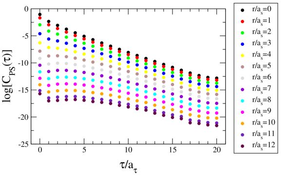
Figure 2: Local-extended charmonium correlators for the PS channel for all possible on-axis separations of the $0.76T_{c}$ ($N_{\tau}=40$) ensemble. Error bars are smaller than the symbols.

The $N_{s}=32$ ensembles, listed in Table 1, provide a means to investigate the volume dependence of the correlators, and hence also that of the potentials. Figure 3 shows the ratio of $N_{s}=24$ to $N_{s}=32$ local-extended correlators for the $1.27T_{c}$ (i.e. the $N_{\tau}=24$) case. From Figure 3, the correlator has no volume dependence for $0\leq r/a_{s}\leq 10$, the $r/a_{s}=11$ case shows some effects and the $r/a_{s}=12$ is clearly highly sensitive to finite volume effects. Consequently, (due to the nearest-neighbour representation of the Laplacian in (9)) we report the potential for $r/a_{s}\leq 9$, i.e. $r\leq 1.1$fm, in the following where it is free from finite volume effects.

We note that the lattice version of the Laplacian in (9) has greatest discretisation error near the origin. Hence we do not include the $r/a_{s}=1$ point in our fits to the potential in section 4.2.

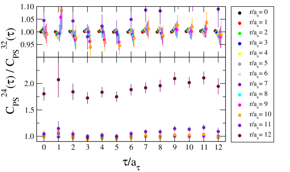
Figure 3: The ratio of the $N_{s}=24$ to $N_{s}=32$ local-extended correlation functions for $1.27T_{c}$ (i.e. $N_{\tau}\!=\!24$). In the lower pane, all separations $0\leq|\mathbf{r}/a_{\tau}|\leq 12$ are shown. The upper pane shows a closeup for $0\leq|\mathbf{r}/a_{\tau}|\leq 10$ with the points shifted horizontally for clarity.

In Figure 4 the PS potential is plotted for the 0.76T_C correlators using the naive time derivative (10) in (8). We note that in the hal qcd method, the potential has a $\tau$ pseudo-dependence which will be averaged over. Figures 5 and 6 show the spatial and temporal contributions of (8) respectively. As can been seen, at large $\tau$ the spatial derivative contribution is stable but the temporal derivative contribution increases near the mid-point of the lattice, $\tau\sim N_{\tau}/2$, which produces a corresponding decrease in the potential at these $\tau$ values in Figure 4. In Figure 7 we use the improved temporal term (11) which clearly resolves the issue for the pseudoscalar case, implying that it was caused by the backward mover as discussed in section 2. We have checked that the same is true in the vector channel. We also note that as $\tau\rightarrow\infty$ there is the expected convergence towards the (negative) value of the PS mass $\eta_{c}=2.9804(1)$GeV Beringer:1900zz . We note that in the region where (8) is valid, i.e. in the absence of a backward mover, $\tilde{E_{0}}$ is equivalent to $\partial C_{\Gamma}/\partial\tau$ only in the limit of negligible excited state contribution. However, noting the very similar small-$\tau$ behaviour in Figures 6 and 7 (where the excited states’ contributions are largest), it is clear that the $\tilde{E_{0}}$ definition works in practice even in the presence of excited states. For these reasons, we will always use the improved temporal form (11) in the following.

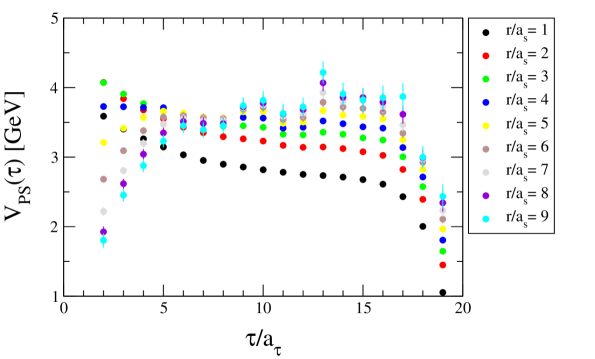
Figure 4: The potential for the $0.76T_{\textrm{C}}$ pseudoscalar channel plotted as a function of $\tau$ for each quark separation $|\mathbf{r}|$, using (8) with the naive time derivative (10).

Figure 5: The spatial contribution, $(1/C_{\Gamma})(\nabla_{r}^{2}C_{\Gamma}/2\mu)$, to the potential (see (8)) for the $0.76T_{\textrm{C}}$ pseudoscalar channel, plotted as a function of $\tau$ for each quark separation $|\mathbf{r}|$.

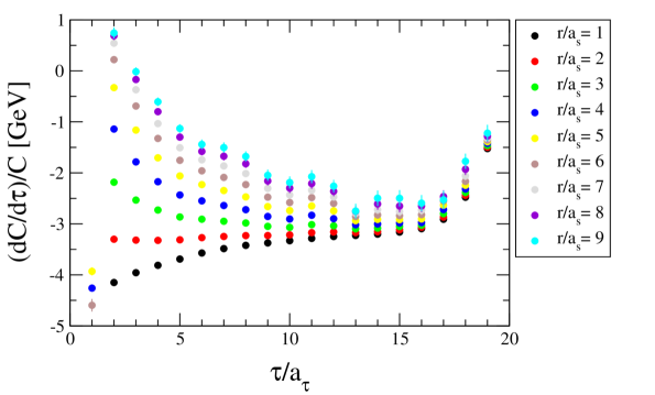
Figure 6: The temporal contribution, $(1/C_{\Gamma})(\partial C_{\Gamma}/\partial\tau)$, to the potential (see (8)), using the naive form, (10), for the $0.76$T${}_{\textrm{C}}$ pseudoscalar channel, plotted as a function of $\tau$ for each quark separation $|\mathbf{r}|$.

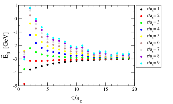
Figure 7: The temporal contribution, $(1/C_{\Gamma})(\partial C_{\Gamma}/\partial\tau)$, to the potential, using the improved temporal form, $\tilde{E_{0}}$, see (11), for the $0.76$T${}_{\textrm{C}}$ pseudoscalar channel for each quark separation $|\mathbf{r}|$.

The central potential is determined by combining the pseudoscalar and vector potentials according to (14) and is shown in Figure 8 for all temperatures. From these figures, it is clear that the 1.52T_C and 1.90T_C data do not stabilise. Hence, we include only the data up to temperatures of 1.27T_C in the following.

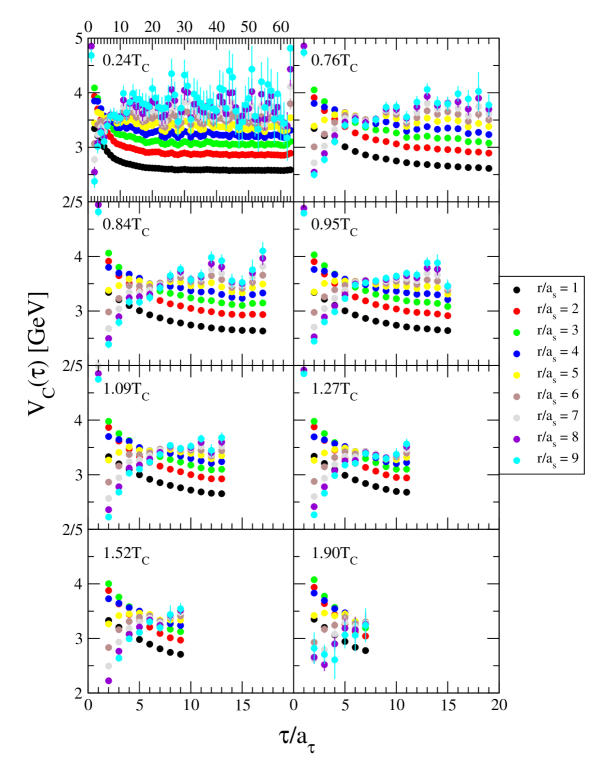
Figure 8: The central potential for all temperatures studied as a function of $\tau$ for each quark separation, $|\mathbf{r}|$.

$T/T_{\rm C}$	$N_{\tau}$	Best range	Lower range
0.24	128	$30-63$	$15-19$
0.76	40	$15-19$	$12-17$
0.84	36	$12-17$	$11-15$
0.95	32	$11-15$	$11-13$
1.09	28	$11-13$	$9-11$
1.27	24	$9-11$	N/A

Table 2: Fitting ranges used to obtain the $\tau-$independent potentials. The “best” range covers the plateau region for each temperature and gives our best fit. The “lower” range is the same as the best range for the next higher temperature, allowing a direct comparison between temperatures.

We remove the $\tau$ pseudo-dependence from the potentials by performing a correlated fit to a constant using the $\tau$ ranges shown in Table 2. Two time ranges are chosen to elucidate the systematic error from the choice of fit range. The “best” range is chosen to be the best available for each temperature, and the “lower” range is chosen to match the best range of the next higher temperature. In this way, direct comparisons can be made between neighbouring temperatures. Using these time ranges, we obtain the temperature-dependent potential shown in Figure 9. The circles correspond to the best range and triangles the lower range. To aid this comparison between temperatures, we include five upper insert plots in Figure 9 which show a closeup of the data at every second separation, i.e. $r=a_{s},3a_{s},\ldots 9a_{s}$. The vertical range of all the insert plots is identical (0.6 GeV). We emphasize from the discussion above, a direct comparison between neighbouring temperatures can be made by comparing the triangles at one temperature with the circles at the next higher temperature. We therefore conclude that the $T\;\raisebox{-2.15277pt}{\hbox to0.0pt{$\sim$\hss}}\raisebox{2.15277pt}{$<$}\;T_{\rm C}$ potentials have no significant temperature effects that our data can discern for any separation, but that there is a significant flattening of the potential at moderate to large separations, $r\;\raisebox{-2.15277pt}{\hbox to0.0pt{$\sim$\hss}}\raisebox{2.15277pt}{$>$}\;0.3$ fm, for $T\;\raisebox{-2.15277pt}{\hbox to0.0pt{$\sim$\hss}}\raisebox{2.15277pt}{$>$}\;T_{\rm C}$.

In Table 3, the central potential values are listed with the systematic (from the $\tau$ fitting procedure described above) and statistical errors combined additively into a single error bar.

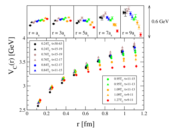
Figure 9: The central potential for various temperatures as a function of separation. Two different $\tau$ ranges were used to estimate the systematic error for all but the largest temperature, see Table 2. The circles represent the “best” fit range in $\tau$ for each temperature, and the triangles the “lower” fit range (which is the next highest temperature’s best range). This allows a direct comparison at different temperatures to be made. The five upper graphs are closeups of the separations $r/a_{s}=1,3,\ldots 9$ with a common vertical range of 0.6 GeV. All points are shifted slightly horizontally for clarity.

$r$ [fm]	$V_{C}$ [GeV]
	$0.24\;T_{C}$	$0.76\;T_{C}$	$0.84\;T_{C}$	$0.95\;T_{C}$	$1.09\;T_{C}$	$1.27\;T_{C}$
0.123	2.58(6)	2.63(3)	2.66(2)	2.67(2)	2.67(5)	2.703(2)
0.246	2.87(6)	2.92(4)	2.95(2)	2.96(2)	2.94(6)	2.967(5)
0.369	3.06(6)	3.12(5)	3.14(1)	3.15(3)	3.11(7)	3.121(7)
0.492	3.23(5)	3.28(5)	3.29(1)	3.29(3)	3.24(6)	3.23(1)
0.615	3.38(3)	3.43(5)	3.42(1)	3.41(4)	3.35(4)	3.30(1)
0.738	3.51(1)	3.55(5)	3.54(2)	3.50(4)	3.43(2)	3.35(2)
0.861	3.63(1)	3.66(5)	3.63(3)	3.58(4)	3.50(2)	3.38(2)
0.984	3.73(3)	3.75(5)	3.72(5)	3.64(4)	3.57(4)	3.40(3)
1.107	3.82(3)	3.85(5)	3.80(6)	3.70(4)	3.64(8)	3.41(3)

Table 3: The central potential data as shown in Figure 10. The statistical uncertainty has been combined additively with the systematic error from the $\tau-$range choice as described in the text, but note that the errors for the $1.27T_{\rm C}$ data are statistical only.

4.2 The Cornell Potential, String Tension and Debye Screening

In Figure 10 the central potential is plotted with the combined statistical and systematic errors as listed in Table 3. For comparison, the Cornell potential Eichten:1974af ; Eichten:1978tg ; Eichten:1979ms ,

$$V(r,T)=-\frac{\alpha_{\rm c}(T)}{r}\;+\;\sigma(T)r\;+\;C,$$ (15)

is also shown using continuum parameters $\alpha_{\rm c}=\pi/12$ Luscher:1980ac and $\sqrt{\sigma}=0.445$ GeV as used in Satz:2005hx (with $C$ adjusted to overlie our data). It was shown in Satz:2005hx that these parameters reproduce the properties of the lowest lying states in both charmonium and bottomonium very accurately. Since our “zero” temperature (i.e. $T=0.24T_{\rm C}$) data follow this established Cornell potential extremely well, they provide strong evidence that our method is extracting the correct physics.

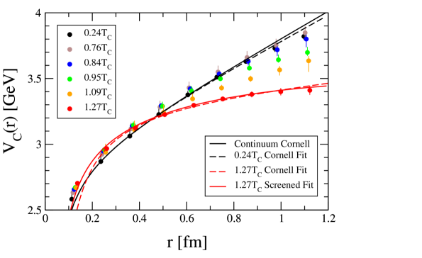
Figure 10: The central potential with combined statistical and systematic errors for various temperatures (noting that the 1.27$T_{\rm C}$ data has statistical errors only). Data points are shifted slightly horizontally for clarity. Examples of the fits to our data are shown using the Cornell (15) and Debye-screened (16) potentials. These used the restricted range $2a_{s}\leq r\leq 9a_{s}$ as described in the text. The Cornell form from (15) with the continuum parameters $\alpha_{\rm c}=\pi/12$ Luscher:1980ac and $\sqrt{\sigma}=0.445$ GeV Satz:2005hx is shown which agrees extremely well with the Cornell fit to our $0.24T_{\rm c}$ data.

The temperature dependence of the central potential is further studied by fitting the $V_{\rm C}$ data to the Cornell function (15) for both the “best and “lower” $\tau$ ranges, see Table 2. We restrict the fit to separations in the range $2a_{s}\leq r\leq 9a_{s}$ due to the systematics at very small and large separations discussed in section 4.1. The parameters from these fits are shown in Table 4 and the resultant string tensions are plotted in Figure 11. We also show the fits in Figure 10 for the coldest and hottest temperatures.

At face value, there is a clear temperature dependence in the string tension as displayed in Figure 11. However, using the strict criteria outlined in section 4.1, the neighbouring temperature’s “best” and “lower” string tensions overlap within errors, and so higher statistics are required to properly decouple this thermal effect from the systematics in this quantity.

A calculation of the string tension at zero temperature was performed in Kawanai:2011jt with nearly physical light dynamical quarks using the hal qcd method, where they found $\sigma=394(7)$ MeV. In studies using the static quark potential, the string tension displays clear temperature effects well below $T_{C}$, see e.g. Cardoso:2011hh (in contrast to Figure 11). However Cardoso:2011hh study pure gauge $SU(3)$ where the confining string tension is essentially an order parameter which is therefore zero for $T>T_{\rm C}$.

In Karsch:1987pv , an alternative to the Cornell potential (15) was proposed for finite temperature where there is colour-Debye screening of the colour sources. This has the form,

$$V(r,T)=-\frac{\alpha_{\rm s}(T)}{r}e^{-m_{D}(T)r}\;+\;\frac{\sigma(T=0)}{m_{D}(T)}\left(1-e^{-m_{D}(T)r}\right)\;+\;C,$$ (16)

where $m_{D}(T)$ is the Debye screening mass. This functional form has the feature that $V(r,T)$ remains finite as $r\rightarrow\infty$.

We have performed fits of the central potential for each temperature using (16) with three fitting parameters, $\alpha,m_{D}$ and $C$. We fixed $\sigma$ to its “zero” temperature value (obtained with our $T=0.24T_{\rm C}$ ensemble) of 434 MeV, see Table 4. As the temperature increases, the screened form, (16), fits the data better than the Cornell form, (15). This can be seen in Figure 10 where both the screened and Cornell fit for the hottest temperature are shown. For the coldest temperature, the screened and Cornell fits are indistinguishable.

The results of these fits are shown in Table 4 and the resultant Debye masses are plotted in Figure 12. At low temperatures, $m_{D}\sim 0$ and it then has a rapid increase around $T_{\rm C}$, in agreement with expectations. In Digal:2005ht , the Debye mass was calculated from a two-flavour lattice calculation of the static quark-antiquark free energy. They found very similar behaviour to Figure 12, with $m_{D}$ increasing rapidly around $T_{\rm C}$ to around 400 MeV at $1.2T_{\rm C}$.

$T/T_{C}$	$\tau$-range	Cornell Fit (15)		Screened Fit (16)
		$\sqrt{\sigma}$	$\alpha_{\rm c}$	$m_{D}$	$\alpha_{\rm s}$
		[MeV]		[MeV]
0.24	30-63	434(7)	0.31(2)	3(8)	0.311(9)
0.24	15-19	390(20)	0.39(5)	50(30)	0.33(3)
0.76	15-19	410(20)	0.36(3)	30(20)	0.34(2)
0.76	12-17	405(14)	0.41(3)	40(20)	0.38(2)
0.84	12-17	378(13)	0.41(3)	70(20)	0.35(2)
0.84	11-15	340(20)	0.46(3)	110(20)	0.36(2)
0.95	11-15	331(11)	0.48(2)	130(20)	0.37(2)
0.95	11-13	340(20)	0.49(3)	120(30)	0.39(2)
1.09	11-13	320(20)	0.43(3)	140(20)	0.31(2)
1.09	9-11	220(20)	0.58(3)	270(30)	0.42(3)
1.27	9-11	180(30)	0.53(3)	340(40)	0.37(3)

Table 4: The results of fitting the central potentials to both the Cornell form, (15), and the Debye-screened form, (16), as described in the text. Note that, following the procedure outlined in section 4.1, two $\tau-$ranges were chosen to allow a direct comparison between neighbouring temperatures.

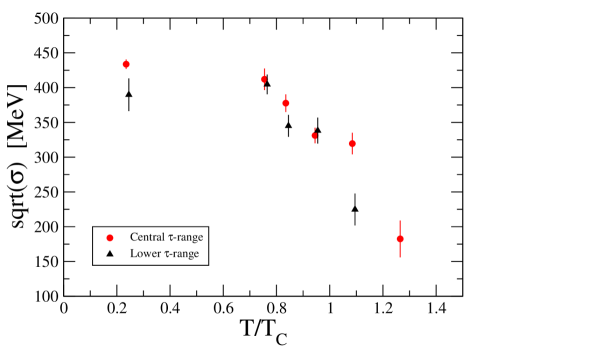
Figure 11: The string tension, $\sigma$, as a function of temperature obtained by fitting the potential data to the Cornell potential (15). Two different $\tau-$ranges “best” and “lower” were also used so that temperature effects can be uncovered, see Table 2. The points are shifted slightly horizontally for clarity.

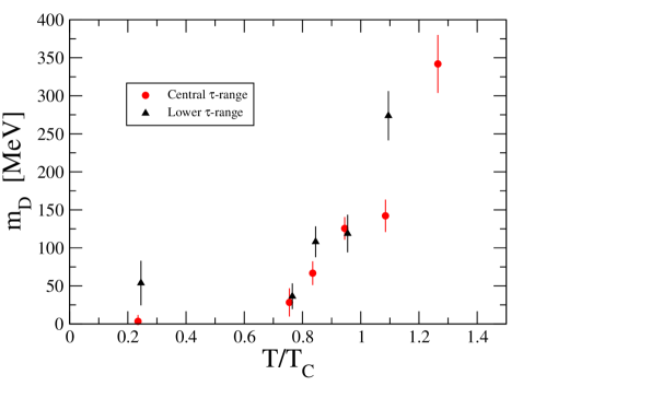
Figure 12: The Debye mass, $m_{D}$, as a function of temperature obtained by fitting the potential data to the screened potential (16). Two different $\tau-$ranges “best” and “lower” were also used so that temperature effects can be uncovered, see Table 2. The points are shifted slightly horizontally for clarity.

4.3 Spin Dependent Potential

We also obtained the ($\tau-$dependent) spin-dependent potentials for the different temperatures by combining the pseudoscalar and vector time-slice potentials from each ensemble according to (14). The $\tau-$dependence was removed using the same procedure as in the central potential case to obtain Figure 13.

Taken at face value, we see a strongly repulsive core, but this has to be qualified by the systematics in the $r/a_{s}=1$ data point as discussed in section 4.1. However, since the spin-dependent potential is the difference, ${V_{V}-V_{PS}}$, the systematics at $r=a_{s}$ may cancel to some extent. Also note that Kawanai:2011xb ; Kawanai:2011fh ; Kawanai:2011jt ; Kawanai:2013aca have found a repulsive core for this potential, but with a quenched calculation. Modelling the interaction via one-gluon exchange, the spin-dependent potential is a $\delta-$function at the origin, so given the body of lattice results including this work, a finite-width, repulsive core appears to be the correct, non-perturbative result. Note also the work of Laschka:2012cf where a finite-width repulsive potential was obtained by including the running of the coupling in one-gluon exchange.

For confined temperatures, $T\;\raisebox{-2.15277pt}{\hbox to0.0pt{$\sim$\hss}}\raisebox{2.15277pt}{$<$}\;T_{C}$, the potential is clearly flat for moderate to large distances with no significant temperature dependence, see Figure 13. In our calculation, as in Kawanai:2011xb ; Kawanai:2011fh the asymptotic value for this confined phase potential is negative. However, when the spin-dependent potential is used to define dynamically the reduced mass, $\mu$, (see (6)) this potential tends to zero at large distances Kawanai:2011jt ; Kawanai:2013aca by definition.

There is a clear temperature effect once the deconfined phase is reached with a distinct minimum at intermediate distances $r\sim 0.4$ fm and significantly larger potential values at large distances $r\;\raisebox{-2.15277pt}{\hbox to0.0pt{$\sim$\hss}}\raisebox{2.15277pt}{$>$}\;0.7$ fm compared to the same potential in the confined phase.

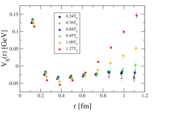
Figure 13: The spin-dependent potential with combined statistical and systematic errors for various temperatures. The points are shifted slightly horizontally for clarity.

4.4 Comparison with other methods

In Figure 14 our central potentials from this work (i.e. using our ${N_{f}=2+1}$ 2nd generation ensembles) are compared with those obtained from our earlier, ${N_{f}=2}$ 1st generation simulations Evans:2013yva . The $N_{f}=2$ potentials were also obtained with the hal qcd time-dependent method, and have been shifted vertically in Figure 14 so that their $r/a_{s}=1$ data points coincide with that of the $0.24T_{\rm C}$ potential. It is encouraging that the potential data points interpolate each other at small $r$, especially given that the lattice parameters and actions used in each simulation are quite different. For a given temperature the ${N_{f}=2+1}$ central potentials are flatter at large $r$ than those from the ${N_{f}=2}$ simulation. This could be due to the inclusion of an extra sea quark that has the ability to screen the strong force between quarks, but further studies would be required to confirm this.

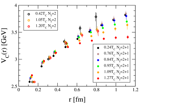
Figure 14: A comparison of the central potentials obtained from this ${N_{f}=2+1}$ work and our earlier ${N_{f}=2}$ simulations Evans:2013yva . The ${N_{f}=2}$ data have two error bars, statistical (left) and systematic (right), and are shifted vertically so that the potential at the first separation agrees with the $N_{f}=2+1$, $0.24T_{C}$ values. All points have been shifted slightly horizontally for clarity.

In Figure 15 we compare the central potentials with the static quark potentials calculated from the Wilson lines Burnier:2014ssa which were also obtained with 2+1 flavours. The static quark potential curves in Figure 15 are shown at the temperatures closest to those in this work, and have been shifted vertically so that their form can be compared to our result. While the higher temperature results agree fairly well between the two approaches, the lower temperature static data are steeper than our results. Further study would be required to determine if this difference is due to Burnier:2014ssa using the infinite quark mass approximation rather than the physical charm quark, or to other systematic differences between the two approaches.

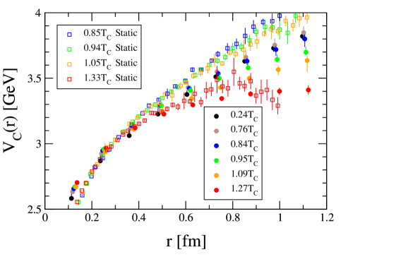
Figure 15: A comparison of the central potential obtained from this work with the static quark potential for comparable temperatures obtained in Burnier:2014ssa . The static potential data have been shifted vertically for the sake of comparison.

5 Conclusions

There is a significant body of theoretical work studying the interquark potential at non-zero temperature using model, perturbative and lattice (non-perturbative) approaches. However, until Iida:2011za ; Evans:2013yva , these lattice studies all used the static quark limit. This work improves upon these static calculations by considering quarks with finite mass, and thus represents a first-principles calculation of the charmonium potential of QCD at non-zero temperature. The method we used is based on the hal qcd time-dependent approach which obtains the potential directly from local-extended correlators.

We do not observe any significant temperature dependence of the central potential below $T_{C}$, while there is a significant flattening above $T_{C}$, consistent with the expectation that the potential becomes deconfining. The string tension is calculated and we find a slower variation of this quantity with temperature than that found using the static quark approximation. Using the Debye-screened form for the potential (which fits our data better than the Cornell form), we determine the Debye mass which is found to be very small at low temperatures and then increase rapidly around $T_{\rm C}$. This is, as far as we know, the first non-perturbative calculation of the Debye mass in charmonium. In the case of the spin-dependent potential, we similarly find no thermal modification for $T\;\raisebox{-2.15277pt}{\hbox to0.0pt{$\sim$\hss}}\raisebox{2.15277pt}{$<$}\;T_{C}$, but a clear variation with temperature at large distances in the deconfined phase and evidence for a repulsive core.

This work improves upon our earlier work Evans:2013yva ; Allton:2013wza by including a dynamical strange quark, and using lattices which are finer, with a larger volume, and have lighter, more physical $u,d$ quarks.

Appendix A Appendix: Momentum Space Propagators

Local-extended correlators can be obtained more efficiently by working with the quark propagators in momentum rather than coordinate space privsin . While this method (which is not our own) has been known for some time and used in many papers which have calculated potentials from the hal qcd method and in studies of multi-baryon states Doi:2012xd , it does not appear to be in any publication, so we outline it here for reference.

For a meson, the local-extended correlator, (3), in the gauge fixed case (with $U(x,x\!+\!\mathbf{r})$ set to unity) can be written,

$$C_{\Gamma}(\mathbf{r},\tau) =-\sum_{\mathbf{x}}\operatorname{T\ \!\!r}\left[D^{-1}(\mathbf{x}\!+\!\mathbf{r},\tau\!:\!\mathbf{0},0)\Gamma D^{-1}(\mathbf{0},0\!:\!\mathbf{x},\tau)\Gamma^{\dagger}\right]$$

$$=-\sum_{\mathbf{x}}\operatorname{T\ \!\!r}\left[D^{-1}(\mathbf{x}\!+\!\mathbf{r},\tau\!:\!\mathbf{0},0)\Gamma\gamma_{5}D^{-1}(\mathbf{x},\tau\!:\!\mathbf{0},0)\gamma_{5}\Gamma^{\dagger}\right]$$ (17)

where $D^{-1}({\rm sink}\!:\!{\rm source})$ is the quark propagator. This correlator can be written in terms of the Fourier transform of the quark propagators,

$$D^{-1}(\mathbf{y},\tau\!:\!\mathbf{0},0)=\frac{1}{V}\sum_{\mathbf{q}}\tilde{D}^{-1}(\mathbf{q})e^{i\mathbf{q}\cdot\mathbf{y}},$$ (18)

giving

$$C_{\Gamma}(\mathbf{r},\tau) =-\frac{1}{V}\sum_{\mathbf{p}}\operatorname{T\ \!\!r}\left[\tilde{D}^{-1}(\mathbf{p})\Gamma\gamma_{5}\tilde{D}^{-1}(-\mathbf{p})\gamma_{5}\Gamma^{\dagger}\right]e^{i\mathbf{p}\cdot\mathbf{r}}$$

$$\equiv\frac{1}{V}\sum_{\mathbf{p}}\tilde{C}(\mathbf{p},\tau)e^{i\mathbf{p}\cdot\mathbf{r}},$$ (19)

where $\tilde{C}(\mathbf{p},\tau)$ is the Fourier transform of the correlator, $C_{\Gamma}(\mathbf{r},\tau)$.

This implies that once $\tilde{C}_{\Gamma}(\mathbf{p},\tau)$ is obtained, then the desired correlator, $C_{\Gamma}(\mathbf{r},\tau)$, can be simply computed for any value of $\mathbf{r}$ using the single sum in (19). This is computationally more efficient than having to perform the trace in (17) for each $\mathbf{x}$ value before then also performing the sum over $\mathbf{x}$.

References

- (1) E. Eichten, K. Gottfried, T. Kinoshita, J. B. Kogut, K. Lane, et al., The spectrum of charmonium, Phys.Rev.Lett. 34 (1975) 369–372.
- (2) E. Eichten, K. Gottfried, T. Kinoshita, K. Lane, and T.-M. Yan, Charmonium: The model, Phys.Rev. D17 (1978) 3090.
- (3) E. Eichten, K. Gottfried, T. Kinoshita, K. Lane, and T.-M. Yan, Charmonium: Comparison with experiment, Phys.Rev. D21 (1980) 203.
- (4) N. Brambilla, A. Pineda, J. Soto, and A. Vairo, Potential NRQCD: An effective theory for heavy quarkonium, Nucl.Phys. B566 (2000) 275, [hep-ph/9907240].
- (5) N. Brambilla, A. Pineda, J. Soto, and A. Vairo, Effective field theories for heavy quarkonium, Rev.Mod.Phys. 77 (2005) 1423, [hep-ph/0410047].
- (6) Y. Ikeda and H. Iida, The anti-quark–quark potential from Bethe–Salpeter amplitudes on lattice, PoS LATTICE2010 (2010) 143, [arXiv:1011.2866].
- (7) Y. Ikeda and H. Iida, Quark-anti-quark potentials from Nambu–Bethe–Salpeter amplitudes on lattice, Prog.Theor.Phys. 128 (2012) 941–954, [arXiv:1102.2097].
- (8) T. Kawanai and S. Sasaki, Interquark potential with finite quark mass from lattice QCD, Phys.Rev.Lett. 107 (2011) 091601, [arXiv:1102.3246].
- (9) T. Kawanai and S. Sasaki, Charmonium potential from full lattice QCD, Phys.Rev. D85 (2012) 091503, [arXiv:1110.0888].
- (10) T. Kawanai and S. Sasaki, Interquark potential for the charmonium system with almost physical quark masses, PoS LATTICE2011 (2011) 126, [arXiv:1111.0256].
- (11) T. Kawanai and S. Sasaki, Heavy quarkonium potential from Bethe–Salpeter wave function on the lattice, Phys.Rev. D89 (2014) 054507, [arXiv:1311.1253].
- (12) N. Ishii, S. Aoki, and T. Hatsuda, The nuclear force from lattice QCD, Phys.Rev.Lett. 99 (2007) 022001, [nucl-th/0611096].
- (13) T. Matsui and H. Satz, suppression by quark-gluon plasma formation, Phys. Lett. B178 (1986) 416.
- (14) NA50 Collaboration Collaboration, M. Abreu et al., Evidence for deconfinement of quarks and gluons from the suppression pattern measured in Pb+Pb collisions at the CERN SPS, Phys.Lett. B477 (2000) 28–36.
- (15) CMS Collaboration Collaboration, S. Chatrchyan et al., Suppression of non-prompt , prompt , and (1S) in PbPb collisions at TeV, JHEP 1205 (2012) 063, [arXiv:1201.5069].
- (16) PHENIX Collaboration, K. Adcox et al., Formation of dense partonic matter in relativistic nucleus-nucleus collisions at RHIC: Experimental evaluation by the PHENIX collaboration, Nucl.Phys. A757 (2005) 184–283, [nucl-ex/0410003].
- (17) STAR Collaboration, J. Adams et al., Experimental and theoretical challenges in the search for the quark gluon plasma: The STAR collaboration’s critical assessment of the evidence from RHIC collisions, Nucl.Phys. A757 (2005) 102–183, [nucl-ex/0501009].
- (18) Á. Mócsy and P. Petreczky, Can quarkonia survive deconfinement?, Phys.Rev. D77 (2008) 014501, [arXiv:0705.2559].
- (19) Á. Mócsy and P. Petreczky, Quarkonia correlators above deconfinement, Phys.Rev. D73 (2006) 074007, [hep-ph/0512156].
- (20) Á. Mócsy and P. Petreczky, Heavy quarkonia survival in potential model, Eur.Phys.J. C43 (2005) 77–80, [hep-ph/0411262].
- (21) O. Kaczmarek and F. Zantow, Static quark anti-quark interactions in zero and finite temperature QCD. i. heavy quark free energies, running coupling and quarkonium binding, Phys.Rev. D71 (2005) 114510, [hep-lat/0503017].
- (22) Z. Fodor, A. Jakovác, S. Katz, and K. Szabo, Static quark free energies at finite temperature, PoS LAT2007 (2007) 196, [arXiv:0710.4119].
- (23) O. Kaczmarek and F. Zantow, Static quark anti-quark interactions at zero and finite temperature QCD. ii. quark anti-quark internal energy and entropy, hep-lat/0506019.
- (24) C.-Y. Wong, Heavy quarkonia in quark-gluon plasma, Phys.Rev. C72 (2005) 034906, [hep-ph/0408020].
- (25) C.-Y. Wong, Effects of dynamical quarks on the stability of heavy quarkonia in quark-gluon plasma, hep-ph/0509088.
- (26) M. Laine, O. Philipsen, P. Romatschke, and M. Tassler, Real-time static potential in hot QCD, JHEP 0703 (2007) 054, [hep-ph/0611300].
- (27) M. Laine, O. Philipsen, and M. Tassler, Thermal imaginary part of a real-time static potential from classical lattice gauge theory simulations, JHEP 0709 (2007) 066, [arXiv:0707.2458].
- (28) A. Rothkopf, T. Hatsuda, and S. Sasaki, Complex heavy-quark potential at finite temperature from lattice QCD, Phys.Rev.Lett. 108 (2012) 162001, [arXiv:1108.1579].
- (29) Y. Burnier and A. Rothkopf, Disentangling the timescales behind the non-perturbative heavy quark potential, Phys.Rev. D86 (2012) 051503, [arXiv:1208.1899].
- (30) A. Bazavov and P. Petreczky, On static quark anti-quark potential at non-zero temperature, Nucl.Phys.A904-905 2013 (2013) 599c–602c, [arXiv:1210.6314].
- (31) A. Bazavov and P. Petreczky, Static quark correlators and quarkonium properties at non-zero temperature, arXiv:1211.5638.
- (32) HAL QCD Collaboration, S. Aoki et al., Lattice QCD approach to nuclear physics, PTEP 2012 (2012) 01A105, [arXiv:1206.5088].
- (33) P. Evans, C. Allton, and J.-I. Skullerud, Ab initio calculation of finite-temperature charmonium potentials, Phys.Rev. D89 (2014), no. 7 071502, [arXiv:1303.5331].
- (34) C. Allton, P. Evans, and J.-I. Skullerud, Charmonium potentials at finite temperature, PoS LATTICE2012 (2012) 082, [arXiv:1306.3140].
- (35) H. Iida and Y. Ikeda, Inter-quark potentials from NBS amplitudes and their applications, PoS LATTICE2011 (2011) 195.
- (36) W. Evans, C. Allton, P. Giudice, and J.-I. Skullerud, Charmonium potentials at non-zero temperature, PoS LATTICE2013 (2014) 168, [arXiv:1309.3415].
- (37) S. Dürr, Physics of with rooted staggered quarks, Phys.Rev. D85 (2012) 114503, [arXiv:1203.2560].
- (38) S. Godfrey and N. Isgur, Mesons in a relativized quark model with chromodynamics, Phys.Rev. D32 (1985) 189–231.
- (39) T. Barnes, S. Godfrey, and E. Swanson, Higher charmonia, Phys.Rev. D72 (2005) 054026, [hep-ph/0505002].
- (40) C. Allton, G. Aarts, A. Amato, W. Evans, P. Giudice, et al., 2+1 flavour thermal studies on an anisotropic lattice, PoS LATTICE2013 (2014) 151, [arXiv:1401.2116].
- (41) R. G. Edwards, B. Joó, and H.-W. Lin, Tuning for three-flavors of anisotropic clover fermions with stout-link smearing, Phys. Rev. D78 (2008) 054501, [hep-lat/0803.3960].
- (42) Hadron Spectrum Collaboration Collaboration, H.-W. Lin et al., First results from 2+1 dynamical quark flavors on an anisotropic lattice: Light-hadron spectroscopy and setting the strange-quark mass, Phys.Rev. D79 (2009) 034502, [arXiv:0810.3588].
- (43) G. Aarts, C. Allton, A. Amato, P. Giudice, S. Hands, and J.-I. Skullerud, Electrical conductivity and charge diffusion in thermal QCD from the lattice, JHEP 1502 (2015) 186, [arXiv:1412.6411].
- (44) Hadron Spectrum Collaboration, L. Liu et al., Excited and exotic charmonium spectroscopy from lattice QCD, JHEP 1207 (2012) 126, [arXiv:1204.5425].
- (45) R. Hudspith, Fourier accelerated conjugate gradient lattice gauge fixing, arXiv:1405.5812.
- (46) SciDAC, LHPC, UKQCD Collaboration, R. G. Edwards and B. Joó, The Chroma software system for lattice QCD, Nucl.Phys.Proc.Suppl. 140 (2005) 832, [hep-lat/0409003].
- (47) Particle Data Group Collaboration, J. Beringer et al., Review of particle physics (RPP), Phys.Rev. D86 (2012) 010001.
- (48) M. Lüscher, Symmetry breaking aspects of the roughening transition in gauge theories, Nucl.Phys. B180 (1981) 317.
- (49) H. Satz, Colour deconfinement and quarkonium binding, J.Phys. G32 (2006) R25, [hep-ph/0512217].
- (50) N. Cardoso and P. Bicudo, Lattice QCD computation of the SU(3) string tension critical curve, Phys.Rev. D85 (2012) 077501, [arXiv:1111.1317].
- (51) F. Karsch, M. Mehr, and H. Satz, Color screening and deconfinement for bound states of heavy quarks, Z.Phys. C37 (1988) 617.
- (52) S. Digal, O. Kaczmarek, F. Karsch, and H. Satz, Heavy quark interactions in finite temperature QCD, Eur.Phys.J. C43 (2005) 71–75, [hep-ph/0505193].
- (53) A. Laschka, N. Kaiser, and W. Weise, Charmonium potentials: Matching perturbative and lattice QCD, Phys.Lett. B715 (2012) 190–193, [arXiv:1205.3390].
- (54) Y. Burnier, O. Kaczmarek, and A. Rothkopf, Static quark-antiquark potential in the quark-gluon plasma from lattice QCD, Phys.Rev.Lett. 114 (2015), no. 8 082001, [arXiv:1410.2546].
- (55) S. Aoki, 2012. Private Communication.
- (56) T. Doi and M. G. Endres, Unified contraction algorithm for multi-baryon correlators on the lattice, Comput.Phys.Commun. 184 (2013) 117, [arXiv:1205.0585].