Towards Optimal Adaptive Wireless Communications in Unknown Environments

Abstract

Designing efficient channel access schemes for wireless communications without any prior knowledge about the nature of environments has been a very challenging issue, in which the channel state distribution of all spectrum resources could be entirely or partially stochastic or adversarial at different time and locations. In this paper, we propose an online learning algorithm for adaptive channel access of wireless communications in unknown environments based on the theory of multi-armed bandits (MAB) problems. By automatically tuning two control parameters, i.e., learning rate and exploration probability, our algorithms could find the optimal channel access strategies and achieve the almost optimal learning performance over time in different scenarios. The quantitative performance studies indicate the superior throughput gain when compared with previous solutions and the flexibility of our algorithm in practice, which is resilient to both oblivious and adaptive jamming attacks with different intelligence and attacking strength that ranges from no-attack to the full-attack of all spectrum resources. We conduct extensive simulations to validate our theoretical analysis.

I Introduction

The design of channel access schemes is a pivotal problem in wireless communications. Stimulated by the recent appearance of smart wireless devices with adaptive and learning abilities, modern wireless communications have raised very high requirements to its solutions, especially in complex environments, where accurate instant channel states can barely be acquired before transmission and long term channel evolution process are unknown (e.g., cognitive radio, smart vehicular and military communications). Thus, it is critical for wireless devices to learn and select the best channels to access in general unknown wireless environments.

Many recent works have tackled the channel access problem in unknown environments by online learning approaches, almost all of which are well formulated as the Multi-armed bandit (MAB) problem [1] due to its inherent capability in keeping a good balance between “exploitation” and “exploration” for the selection of channels and the superior throughput gain with the finite-time optimality guarantee, e.g., [2, 3, 4, 5, 6, 7, 8, 9, 10, 12, 11, 13]. The main goal is to find a channel access strategy that achieves the optimal expected throughput by minimizing the term “regret” as learning performance metric, i.e., the performance gap between the proposed strategy and the optimal fixed one known in hindsight, accumulated over time. Briefly speaking, these works can be categorized into two different types of MAB models, namely, adversarial (non-stochastic) MAB [2, 3, 4][10, 11] and stochastic MAB [5, 6, 8, 7, 9] [12, 13]. Stochastic MAB assumes that the channel state follows some unknown i.i.d. process, while adversarial MAB assumes that the channel state can be controlled arbitrarily by adversaries (e.g., jamming attackers) where its distribution is not i.i.d (i.e., non-i.i.d.) any more. Accordingly, the analytic approaches and performance results of the two models are distinctively different. A well-known truth is that stochastic MAB and adversarial MAB have regrets of order “logarithmic-t” [18] and “root-t” [19] over time $t$, respectively. Obviously, the learning performance of the stochastic MAB highly outperforms that of the adversarial MAB.

As we know, one key assumption of almost all existing works is the nature of environments, as a known prior, is either stochastic or adversarial. This is limited in describing general wireless environments in practice, although it largely captures the main characteristic of them. Because, in many practical wireless applications, the nature of the environment is not restricted to either the stochastic or the adversarial type, and it usually can not be known in advance.

On the one hand, the application of existing models may lead to bad learning performance when no prior about the environment is available. Consider a wireless network deployed in a potentially hostile environment. The number and locations of attackers are often unrevealed to the wireless networks. In this scenario, most likely, certain portions of spatially-dispersed channels may (or may not) suffer from denial of service attackers that are adversarial, while others are stochastic distributed. Compared with the classic mind that uses the adversarial MAB model [2, 3, 4][10, 11], here to design optimal channel access strategies, the use of the stochastic MAB may not be feasible due to the existence of adversaries. Meanwhile, the use of the adversarial MAB model on all channels will lead to large values of regret, since a great portion of channels can still be stochastically distributed. Thus, it is hard to decide the type of MAB models to be used in the first place.

On the other hand, the channel access strategy based on stochastic MAB model [5, 6, 8, 7, 9] [12, 13] will face practical implementation issues, even though it is certain that there is no long term adversarial behavior. In almost all wireless communication systems, the commonly seen occasionally disturbing events would make the stochastic channel distributions contaminated. These include the burst movements of individuals, the jitter effects of electronmagnetic waves, and the seldom but irregular replacement of obstacles, etc. In this case, the channel distribution will not follow an i.i.d. process for a small portion of time during the whole learning period. Thus, whether the stochastic MAB theory is still applicable, how the contamination affects the learning performance and to what extend the contamination is negligible are not clear to us. Therefore, the design of a unified channel access scheme without any prior knowledge of the operating environment is very challenging. It is highly desirable and bears great theoretical value.

In this paper, we propose a novel adaptive multi-channel access algorithm for wireless communications that achieves near-optimal learning performance without any prior knowledge about the nature of the environment, which provides the first theoretical foundation of scheme design and performance characterization for this challenging issue. The proposed algorithm neither needs to distinguish the stochastic and adversarial MAB problems nor requires the time horizon for run. To the best of our knowledge, ours is the first work that bridges the stochastic and adversarial MABs into a unified framework with promising applications in practical wireless systems.

The idea is based on the famous EXP3 [19] algorithm in the non-stochastic MAB by introducing a new control parameter into the exploration probability for each channel. By joint control of learning rate and exploration probability, the proposed algorithm achieves almost optimal learning performance in different regimes. When the environment happens to be adversarial, our proposed algorithm enjoys the same behavior as classic adversarial MABs-based algorithms and has the optimal regret“root-t” bound in the adversarial regime. When the environment happens to be stochastic, we indicate a problem-dependent “polylogarithmic-t” regret bound, which is slightly worse than the optimal “logarithmic” bound in [18]. Furthermore, we prove that the proposed algorithm retains the “polylogarithmic-t” regret bound in the stochastic regime as long as on average the contamination over all channels does not reduce the gap $\Delta$ between the optimal and suboptimal channels by more than a half. Note that all regret bounds are sublinear to time horizon, which indicates the optimal channel access strategy is achievable. Our main contributions are summarized as follows.

1) We categorize the features of the general wireless communication environments mainly into four typical regimes: the adversarial regime, the stochastic regime, the mixed adversarial and stochastic regime, and the contaminated stochastic regime. We provide solid theoretical results for them, each of which achieves the almost optimal regret bounds.

2) Our proposed AUFH-EXP3++ algorithm considers the statistical information sharing of a channel that belongs to different transmission strategies, which can be regarded as a special type of combinatorial semi-bandit problem. In this scenario, given the size of all channels $n$ and the number of receiving channels $k_{r}$, AUFH-EXP3++ achieves the regret of order $O({k_{r}}\sqrt{tn\ln n})$ in the adversarial regime (for usually considered oblivious adversary) and the regret of order $\tilde{O}(\frac{{n{k_{r}}\log{{(t)}}}}{\Delta})$ in other stochastic regime up to time $t$. From the perspective of parameters $n$ and $k_{r}$ for different configurations of wireless communications, AUFH-EXP3++ achieves tight regret bound in both the adversarial setting [32] and the stochastic setting [29]. We also study the performance of our algorithm under adaptive adversary for the first time.

3) We provide a computational efficient enhanced version of the AUFH-EXP3++ algorithm. Our algorithm enjoys linear time and space complexity in terms of $n$ and $k_{r}$ that indicates very good scalability, which can be implemented in large scale wireless communication networks.

4) We conduct plenty of diversified numerical experiments, and simulation results demonstrate that all advantages of the AUFH-EXP3++ algorithm in our theoretical analysis is real and can be implemented easily in practice.

The rest of this paper is organized as follows: Related works are discussed in Section II. Section III describes the communication model, problem formulation, and the four regimes. Section IV introduces the optimal adaptive uncoordinated frequency hopping algorithm, AUFH-EXP3++. The performance results for different regimes are presented in Section V, while their theoretical proofs are shown in Section VI. Section VII presents a computational efficient implementation of the AUFH-EXP3++ algorithm. Numerical and simulation results are available in Section VIII. Finally, we conclude the paper in Section IX.

II Related Works

Recently, online learning-based approaches to address wireless communications and networking problems in unknown environments have gained growing attention. The characteristics of learning by repeated interactions with environments are usually categorized into the domain of reinforcement learning (RL). It is worth pointing out that there exists extensive literature in RL, which generally target at a broader set of learning problems in Markov Decision Processes (MDPs) [33]. As we know, such learning algorithms can guarantee optimally only asymptotically to infinity, which cannot be relied upon in mission-critical applications. However, MAB problems constitute a special class of MDPs, for which the regret learning framework is generally viewed as more effective both in terms of convergence and computational complexity. Thus, the use of MAB models is highly identified. The works based on the stochastic MAB model often consider about the stochastically distributed channels in benign environments, such as dynamic spectrum access [6][28][13], cognitive radio networks [5], channel monitoring in infrastructure wireless networks [9][12], wireless scheduling [8], and channel access scheduling in multi-hop wireless networks [7], etc. The adversarial MAB model is applied to adversarial channel conditions, such as the anti-jamming wireless communications [2][3][11], short-path routing [21][31], non-stochastic channel access affected by primary user activity in cognitive radio networks [4] and power control and channel selection problems [10].

The stochastic and adversarial MABs have co-existed in parallel for almost two decades. Only until recently, the attempt of [25] to bring them together did not make it in a full sense of unification, since the algorithm relies on the knowledge of time horizon and makes an one-time irreversible switch between stochastic and adversarial operation modes if the beginning of the play exhibits adversarial behavior. The first practical algorithm for both stochastic and adversarial bandits is proposed in [24]. Our current work uses the idea of introducing the novel exploration parameter $\xi_{t}(f)$ [24] into our own special combinatorial exponentially weight algorithm by exploiting the channel dependency among different strategies.

This new framework avoids the computational inefficiency issue for general combinatorial adversary bandit problems as indicated in [7] [22]. It achieves a regret bound of order $O({k_{r}}\sqrt{tn\ln n})$, which only has a factor of $O(\sqrt{k_{r}})$ factor off when compared to the optimal $O(\sqrt{{k_{r}}tn\ln n})$ bound in the combinatorial adversary bandit setting [32]. However, we do believe that the regret bound in our framework is the optimal one for the exponential weight (e.g. EXP3 [19]) type of algorithm settings in the sense that the algorithm is computationally efficient. Thus, our work is also a first computationally efficient combinatorial MAB algorithm for general unknown environment. What is more surprising and encouraging, in the stochastic regimes (including the contaminated stochastic regime), all of our algorithms achieve a regret bound of order $\tilde{O}(\frac{{n{k_{r}}\log{{(t)}}}}{\Delta})$. In the sense of channel numbers $n$ and size of channels within each strategy $k_{r}$, this is the best result for combinatorial stochastic bandit problems [29]. Please note that in [6], they have a regret bound of order ${O}(\frac{{n^{4}\log{{(t)}}}}{\Delta})$; in [14], the regret bound is ${O}(\frac{{n^{3}\log{{(t)}}}}{\Delta})$; and in [15], the regret bound is ${O}(\frac{{n^{2}\log^{3}{{(t)}}}}{\Delta})$. Thus, our proposed algorithms are order optimal with respect to $n$ and ${k_{r}}$ for all different regimes, which indicate the good scalability for general wireless communication systems.

III Problem Formulation

III-A System Model

We consider two wireless devices communicating in an unknown environment, each is within the other device’s transmission range. The sender transmits data packets to the receiver synchronically over time. The wireless environment is highly flexible in dynamics, where states of the channels could follow different stochastic distributions and could also suffer from different kinds of potentially adversarial attacks. They can also vary over different time slots and channel sets. Without loss of generality (w.l.o.g.), we consider the jamming attack as the representative adversarial model. Specifically, we will categorize the feature of wireless communication environments into four typical regimes in our next discussions. The transceiver pair selects multiple channels to send and receive signals over a set of $n$ available orthogonal channels with possibly different data rates across them. We do not differentiate channels and frequencies in our discussion. During each time slot, the transmitter chooses $k_{t}$ out of $n$ channels to transmit data and the receiver chooses $k_{r}$ out of $n$ channels to receive data. We assume the transmitter and receiver do not pre-share any secrets with each other before data communication, and there is no feedback channel from the receiver to the transmitter. We assume one jammer launches attack to the transceiver pair over $n$ channels, and the jammer does not have the knowledge about the transceiver’s strategies before data communication. The data packets rate at time slot $t$ from the transmitter on channel $f$ is denoted by $g_{t}(f)$, $g_{t}(f)\in[0,M]$. Here constant $M$ is the maximum data rate for all channels.

III-B The Adaptive Uncoordinated Frequency Hopping Problem

Since no secret is shared and no adversarial event is informed to the transceiver pair, the multi-channel wireless communications in unknown environments are necessary to use frequency hopping strategies to dynamically select a subset of channels to maximize its accumulated data rates over time. We name ours as the Adaptive Uncoordinated Frequency Hopping (AUFH) protocol due to its flexibility to achieve optimal performance in various scenarios, when compared to the recent and sophisticated developed UFH protocol in [2][11]. Here the receiver’s selection of the frequency hopping strategy to maximize the cumulated data packets reception has the following challenge: 1) it does not know the transmitter and adversarial events in the environment, thus it has no good channel access strategy to begin with; 2) the receiver is desirable to have an adaptively optimal channel access strategy in all different situations.

We consider the AUFH problem as a sequential decision problem, where the choice of receiving channels at each time slot is a decision. Denote $\{0,1\}^{n}$ as the vector space of all $n$ channels. The strategy space for the transmitter is denoted as $S_{t}\subseteq\{0,1\}^{n}$ of size $\binom{n}{k_{t}}$, and the receiver’s is denoted as $S_{r}\subseteq\{0,1\}^{n}$ of size $\binom{n}{k_{r}}$. If the $f^{th}$-channel is selected for transmitting and receiving data, the value of the $f$-th entry of a vector (channel access strategy) is $1$, and 0 otherwise. In the case of the existence of jamming attack on a subset of $k_{j}$ channels, the strategy space for the jammer is denoted as $S_{j}\subseteq\{0,1\}^{n}$ of size $\binom{n}{k_{j}}$. For convenience, we say that the $f$-th channel is jammed if the value of $f$-th entry is 0 and otherwise is 1. At each time slot, after choosing a strategy $s_{r}$, the value of the data rate (or called “reward”) $g_{t}(f)$ is revealed to the receiver if and only if $f$ is chosen as a receiving channel.

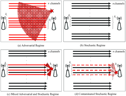
Figure 1: Multi-channel Wireless Communications in Different Regimes

Formally, the frequency hopping multi-channel access game can be formulated as a MAB problem that is described as follows: at each time slot $t=1,2,3,...$, the receiver as a decision maker select a strategy $I_{t}$ from $S_{r}$. The cardinality of $S_{r}$ is $|S_{r}|=N$. The reward $g_{t}(f)$ is assigned to each channel $f\in\{1,...,n\}$ and the receiver only get rewards in strategy $i\in S_{r}$. Note that $I_{t}$ denotes a particular strategy chosen at time slot $t$ from the receiver’s strategy set $S_{r}$, and $i$ denotes a strategy in $S_{r}$. The total reward of a strategy $i$ in time slot $t$ is ${g_{t}(i)}=\sum\nolimits_{f\in i}{{g_{t}(f)}}$. Then, on the one hand, the cumulative reward up to time slot $t$ of the strategy $i$ is ${G_{t}(i)}=\sum\nolimits_{s=1}^{t}{{g_{s}(i)}}=\sum\nolimits_{f\in i}{\sum\nolimits_{s=1}^{t}{{g_{s}(f)}}}.$ On the other hand, the total reward over all the chosen strategies by the receiver up to time slot $t$ is ${\hat{G}_{t}}=\sum\nolimits_{s=1}^{t}{{g_{s}(I_{s})}}=\sum\nolimits_{s=1}^{t}{\sum\nolimits_{f\in{I_{s}}}{{g_{s}(f)}}}$, where the strategy $I_{s}$ is chosen randomly according to some distribution over $S_{r}$. The performance of this algorithm is qualified by regret $R(t)$, defined as the difference between the expected number of successfully received data packets using our proposed algorithm and the expected rewards that use the best fixed solution up to $t$ time slots for the game, i.e.,

$$R(t)=\mathop{\max}\limits_{i\in{S_{r}}}\mathbb{E}\left\{{{G_{t}(i)}}\right\}-\mathbb{E}\left[{{{\hat{G}}_{t}}}\right],$$ (1)

where the maximum is taken over all available strategies to the receiver. However, during the theoretical analysis of the AUFH-based algorithm in our next discussion, if we use the gain (reward) model, we have to apply additional smoothing of the playing distribution $q_{t}(f)$ regarding $\tilde{g}_{t}(f)$. Thus, we can introduce the loss model by the simple trick of $\ell_{t}(f)=1-g_{t}(f)$ for each channel $f$ and $\ell_{t}(i)=k_{r}-g_{t}(i)$ for each strategy, respectively. Then, we have $L_{t}(i)=tk_{r}-G_{t}(i)$ where ${L_{t}}(i)=\sum\nolimits_{s=1}^{t}\ell_{t}(i)={\sum\nolimits_{s=1}^{t}{\sum\nolimits_{f\in i}{{\ell_{s}(f)}}}}$, and similarly, we have $\hat{L}_{t}=tk_{r}-\hat{G}_{t}$. We use $\mathbb{E}_{t}[\cdot]$ to denote expectations on realization of all strategies as random variables up to round $t$. Therefore, the expected regret $R(t)$ can be rewritten as

$$\begin{array}[]{l}\!\!\!\!\!\!\!\!\!\mathbb{E}\left[{{{\hat{L}}_{t}}}\right]-\mathop{\min}\limits_{i\in{S_{r}}}\mathbb{E}\left\{{{L_{t}(i)}}\right\}=\mathbb{E}\sum\limits_{s=1}^{t}{{\ell_{t}}({I_{t}})}-\mathop{\min}\limits_{i\in{S_{r}}}\mathbb{E}\sum\limits_{s=1}^{t}{{\ell_{t}}(i)}\\ =\mathbb{E}[\sum\limits_{s=1}^{t}{\mathbb{E}_{s}[{\sum\limits_{f\in{I_{s}}}{{\ell_{s}(f)}}}]}]-\mathop{\min}\limits_{i\in{S_{r}}}({\mathbb{E}[{\sum\limits_{s=1}^{t}\mathbb{E}_{s}[{\sum\limits_{f\in i}{{\ell_{s}(f)}}}]}\!\!]}).\end{array}$$

The expectation is taken over the possible randomness of the proposed algorithm and loss generation model. The goal of the algorithm is to minimize the regret. The above definition of regret is usually named as the pseudo regret [1], which is upper bounded by the expected regret $\mathbb{E}\{\bar{R}(t)\}=\mathbb{E}\{\sum\nolimits_{s=1}^{t}{{\ell_{t}}({I_{t}})}-\mathop{\min}\nolimits_{i\in{S_{r}}}\sum\nolimits_{s=1}^{t}{{\ell_{t}}(i)}\}$. Only when the adversary is oblivious, who prepares the entire sequence of loss functions ${\ell_{t}}({I_{t}})$ ($t=1,2,3,...$) in advance, pseudo regret (III-B) coincides with the standard expected regret $\mathbb{E}\{\bar{R}(t)\}$[1].

Note that the choice of the loss function at time slot $t$ of the oblivious adversary is independent to the first $t-1$ time slots. Otherwise, the adversary can be called an adaptive adversary. In this case, let us denote the decision maker’s entire sequence of strategies up to current timslot $t$ as $(I_{1},...,I_{t})$, which we abbreviate by $I_{1,...,t}$. The expected cumulative loss suffered by the player after $t$ rounds is $\mathbb{E}[{\sum\nolimits_{s=1}^{t}{{\ell_{s}}({I_{1,...,s}})}}]$. We need to compare it with a competitor class $\mathcal{C}_{t}$, which is simply a set of deterministic strategy sequences of length $t$. Intuitively, we would like to compare the decision maker’s loss with the cumulative loss of the best action sequence in $\mathcal{C}_{t}$. In practice, the most common way to evaluate the decision maker’s performance is to measure its external pseudo-regret compared to $\mathcal{C}_{t}$ [19]. Thus, the regret for adaptive adversary is defined as,

$$\!\!\!\!\!R(t)\!\!=\mathop{\max}\limits_{({y_{1}},...,{y_{t}})\in{\mathcal{C}_{t}}}\mathbb{E}[\!{\sum\limits_{s=1}^{t}{({{\ell_{s}}({I_{1,...,s}})-{\ell_{s}}({I_{1,...,s-1}},{y_{s}})})}}].$$ (3)

This regret definition is suitable for most of the theoretical works of the online learning and bandit setting. If the adversary is oblivious, we have ${{\ell_{t}}({I_{1,...,t}})}$ equals to ${{\ell_{t}}({I_{t}})}$. With this simplified notation, the regret in (3) becomes

$$\mathds{E}[{\sum\limits_{s=1}^{t}{{\ell_{s}}({I_{s}})}}]-\mathop{\min}\limits_{({y_{1}},...,{y_{t}})\in{\mathcal{C}_{t}}}\sum\limits_{s=1}^{t}{{\ell_{s}}({y_{s}})},$$

which is exactly the same as (III-B) with $\mathcal{C}_{t}=S_{r}$, if we take an expectation over all the strategy sequence $({y_{1}},...,{y_{t}})$.

III-C The Four Regimes of Wireless Environments

Since our algorithm does not need to know the nature of the environments, there exist different features of the environments that will affect its performance. We categorize them into the four typical regimes as shown in Fig. 1.

III-C1 Adversarial Regime

In this regime, there is a jammer sending interfering power or injecting garbage data packets over all $n$ channels such that the transceiver’s channel rewards are completely suffered by an unrestricted jammer (See Fig.1 (a)). When we assume the use of the same level of transmission power as in the stochastic regime, the data rate will be significantly reduced in the adversarial regime. Note that, as a classic model of the well known non-stochastic MAB problem [19], the adversarial regime implies that the jammer often launches attack in almost every time slot. It is the most general setting and the other three regimes can be regarded as special cases of the adversarial regime. Obviously, a strategy $i\in\mathop{\arg\min}\nolimits_{i^{\prime}\in{S_{r}}}\{{\mathbb{E}[{\sum\nolimits_{s=1}^{t}{{L_{t}}(i^{\prime})}}]}\}$ is known as a best strategy in hindsight for the first $t$ round.

Attack Model: Different attack philosophies will lead to different level of effectiveness. We classify various types of jammers into the following two categories in the adversarial regime:

a) Oblivious jammer: an oblivious jammer could attack different channels with different jamming strength as a result of different data rate reductions. Its current attacking strategy is not based the observed past communication records. As described in [11], oblivious jammer can use static and random strategies to attack wireless channels. If its attacking strategy is time-independent (e.g. static jammer), we can simply regard it as a stochastic channel with bad channel quality. Usually, the attacking strategy for oblivious jammer can change with time. As noticed, many other kinds of jammers, such as partial band jamming, sweep jamming etc. [26] all belong to the oblivious attack model. Briefly, it is a simple attack model that does not react to the defending algorithm, although the attackers’ attacking strategies could be largely different.

b) Adaptive jammer: an adaptive jammer, also named as non-oblivious jammer, adaptively selects its jamming strength on the targeted (sub)set of jamming channels by utilizing its past experience and observation of the previous communication records. In the adversarial regime, we consider that the adaptive jammer is very powerful in the sense that it does not only know the communication protocol and able to attack with different level of strength over a subset of channels for data communications during a single time slot, but it also can monitor all the $n$ available channels during the same time slot. For example, the reactive jammer with the behavior described in [26] belongs to this type. As shown in a recent work[16], no bandit algorithm can guarantee a sublinear regret $o(t)$ against an adaptive adversary with unbounded memory. The adaptive adversary can mimic and perform the same learning algorithm as the decision maker, i.e., the receiver in our work. It can set the same channel access probabilities as the channel access algorithm, which will lead to a linear regret. Therefore, we consider a more practical m-memory-bounded adaptive adversary [16] model, which is constrained to choose loss functions that depend only on the $m+1$ most recent strategies.

III-C2 Stochastic Regime

In this regime, the transceiver communicates over $n$ stochastic channels as shown in Fig.1 (b). The channel losses $\ell_{t}(f),\forall f\in 1,...,n$ (Obtained by transferring the reward to loss $\ell_{t}(f)=1-g_{t}(f)$) of each channel $f$ are sampled independently from an unknown distribution that depends on $f$, but not on $t$. We use $\mu_{f}=\mathbb{E}\left[{{\ell_{t}(f)}}\right]$ to denote the expected loss of channel $f$. We define channel $f$ as the best channel if $\mu(f)={\min_{f^{\prime}}}\{{\mu(f^{\prime})}\}$ and suboptimal channel otherwise; let $f^{*}$ denote some best channel. Similarly, for each strategy $i\in S_{r}$, we have the best strategy $\mu(i)={\min_{i^{\prime}}}\{{\sum\nolimits_{f\in i^{\prime}}{\mu(f)}}\}$ and suboptimal strategy otherwise; let $i^{*}$ denote some best strategy. For each channel $f$, we define the gap $\Delta(f)=\mu(f)-\mu({f^{*}})$; let $\Delta_{f}={\min_{f:\Delta(f)>0}}\left\{{\Delta(f)}\right\}$ denote the minimal gap of channels, or the gap from the second best channel(s). Similarly, for each strategy $i$, we have $\Delta(i)=\mu(i)-\mu({i^{*}})$; let $\Delta_{i}={\min_{i:\Delta(i)>0}}\left\{{\Delta(i)}\right\}$ denote the minimal gap of strategies. Let $N_{t}(f)$ and $N_{t}(i)$ be the respective number of times channel $f$ and strategy $i$ was played up to time $t$, the regret can be rewritten as $\tilde{R}(t)$ based on $N_{t}(f)$, and we have

$$R(t)=\sum\limits_{i}{\mathbb{E}\left[{{N_{t}}(i)}\right]}\Delta(i)\leq\tilde{R}(t)=\sum\limits_{f}{\mathbb{E}\left[{{N_{t}}(f)}\right]}\Delta(f).$$ (4)

Note that we calculate the upper bound regret $\tilde{R}(n)$ from the perspective of channel set $\mathcal{K}$, where the regret is upper bounded by the regret from the perspective of strategies set $\mathcal{N}$. This is because the set of strategies is of the size $\binom{n}{k_{r}}$ that grows exponentially with respect to $n$ and it does not exploit the channel dependency among different strategies. We thus calculate the upper regret from the perspective of channels, where tight regret bounds are achievable.

III-C3 Mixed Adversarial and Stochastic Regime

This regime assumes that the jammer only attack $k_{j}$ out $n$ channels at each time slot. As shown in Fig.1 (c), there is always a $k_{j}/n$ portion of channels that suffers from jamming attack while the other $(n-k_{j})/n$ portion is stochastically distributed. We call this regime the mixed adversarial and stochastic regime.

Attack Model: We consider the same type of jammer as described in the adversarial regime for the mixed adversarial and stochastic regime, which includes: static jamming and random jamming of the oblivious jammer and the adaptive jammer. The difference here is that the jammer only attacks a subset of channels of size $k_{j}$ over the total $n$ channels not all channels.

III-C4 Contaminated Stochastic Regime

The definition of the contaminated stochastic regime comes from many practical observations that only a few channels and time slots are exposed to adversary. Here comes the question: is this environment still stochastic or adversarial? We are fortunate to answer this question. In this regime, for oblivious jammer, it selects some slot-channel pairs $(t,f)$ as “locations” to attack before the multi-channel wireless communications start, while the remaining channel rewards are generated the same as the stochastic regime. We can introduce and define the attacking strength parameter $\zeta\in[0,1/4)$. After certain $\tau$ timslots, for all $t>\tau$ the total number of contaminated locations of each suboptimal channel up to time $t$ is $t\Delta(f)\zeta$ and the number of contaminated locations of each best channel is $t\Delta_{f}\zeta$.

We call a contaminated stochastic regime moderately contaminated, if by the definition $\zeta$ is at most $1/4$, we can prove that for all $t>\tau$ on the average over the stochasticity of the loss sequence the adversary can reduce the gap of every channel by at most one half. Thus, if the attacking strength $\zeta\in[0,1/4]$, the environment can still be regarded as benign that behaves stochastically (though it is contaminated).

Algorithm 1 AUFH-EXP3++: An MAB-based Algorithm for AUFH

  Input: $n,k_{r},t$, and See text for definition of $\eta_{t}$ and $\xi_{t}(f)$.

  Initialization: Set initial channel and strategy losses $\forall i\in[1,N],\tilde{L}_{0}(i)=0$ and $\forall f\in[1,n],\tilde{\ell}_{0}(f)=0$, respectively; Then the initial channel and strategy weights $\forall i\in[1,N],W_{0}(i)=k_{r}$ and $\forall f\in[1,n],w_{0}(f)=1$, respectively. The initial total strategy weight $W_{0}=N=\binom{n}{k_{r}}$. ​

  Set: ​​ $\beta_{t}\!\!=\!\!\frac{1}{2}\sqrt{\frac{{\ln n}}{{tn}}}$; ${\varepsilon_{t}}\left(f\right)\!=\!\min\left\{{\frac{1}{{2n}},{\beta_{t}},{\xi_{t}}\left(f\right)}\right\},\forall f\in\left[{1,n}\right]$.

  for  time slot $t=1,2,...$ do

     1: The receiver selects a channel hopping strategy $I_{t}$ at random according to the strategy’s probability $p_{t}(i),\forall f\in\left[{1,n}\right]$, with $p_{t}(i)$ computed as follows:

$${p_{t}}(i)=\left\{\begin{array}[]{l}\!\!\!\left({1-\sum\nolimits_{f=1}^{n}{{\varepsilon_{t}}(f)}}\right)\frac{{{w_{t-1}}\left(i\right)}}{{{W_{t-1}}}}+\!\sum\limits_{f\in i}{{\varepsilon_{t}}(f)}\ \emph{if}\ i\in\mathcal{C}\\ \!\!\!\left({1-\sum\nolimits_{f=1}^{n}{{\varepsilon_{t}}(f)}}\right)\frac{{{w_{t-1}}\left(i\right)}}{{{W_{t-1}}}}\ \quad\quad\quad\quad\ \text{\emph{if}}\ i\notin\mathcal{C}\end{array}\right.$$

The computation is taken for the probability distributions over all strategies $p_{t}=(p_{t}(1),p_{t}(2),...,p_{t}(N))$.

     2: The receiver computes the probability $q_{t}(f),\forall f\in\left[{1,n}\right]$, as

$$\begin{array}[]{l}{q_{t}}(f)=\sum\limits_{i:f\in i}{{p_{t}}(i)}=\left({1-\sum\nolimits_{f=1}^{n}{{\varepsilon_{t}}(f)}}\right)\frac{{\sum\nolimits_{i:f\in i}{{w_{t-1}}\left(i\right)}}}{{{W_{t-1}}}}\\ \quad\quad\quad\quad\quad\quad\quad\quad\ \ +\sum\limits_{f\in i}{{\varepsilon_{t}}(f)}\left|{\left\{{i\in\mathcal{C}:f\in i}\right\}}\right|.\end{array}$$

Then, the probability distributions over all channels are $q_{t}=(q_{t}(1),q_{t}(2),...,q_{t}(n))$.

     3: The receiver calculates the loss for channel $f$, $\ell_{t-1}(f),\forall f\in I_{t}$ based on the received channel gain $g_{t-1}(f)$ by using $\ell_{t-1}(f)=1-g_{t-1}(f)$. Compute the estimated loss $\tilde{\ell}_{t}(f),\forall f\in[1,n]$ as follows:

$${\tilde{\ell}_{t}}(f)=\left\{\begin{array}[]{l}\frac{{{\ell_{t}}(f)}}{{{q_{t}}(f)}}\quad\text{\emph{if channel}}f\in{I_{t}}\\ 0\ \ \quad\quad\emph{otherwise}.\end{array}\right.$$

     4: The receiver updates all the weights as

$$\begin{array}[]{l}\begin{array}[]{l}{w_{t}}\left(f\right)={w_{t-1}}\left(f\right){e^{-\eta_{t}{{\tilde{\ell}}_{t}}(f)}}={e^{-\eta_{t}{{\tilde{L}}_{t}}(f)}}.\\ {{\bar{w}}_{t}}\left(i\right)=\prod\limits_{f\in i}{{w_{t}}(f)}={{\bar{w}}_{t-1}}\left(i\right){e^{-\eta_{t}{{\tilde{\ell}}_{t}}(i)}}.\end{array}\end{array}$$

where ${{\tilde{L}}_{t}}(f)={{\tilde{L}}_{t-1}}(f)+{{\tilde{\ell}}_{t-1}}(f),{{\tilde{\ell}}_{t-1}}(e)=\sum\nolimits_{f\in i}{{{\tilde{\ell}}_{t-1}}(f)}$ and ${{\tilde{L}}_{t}}(i)={{\tilde{L}}_{t-1}}(i)+{{\tilde{\ell}}_{t-1}}(i)$. The sum of the total weights of the strategies is

$${W_{t}}=\sum\limits_{i\in S_{r}}{{{\bar{w}}_{t}}\left(i\right)}$$

  end for

IV The Optimal Adaptive Uncoordinated Frequency Hopping Algorithm

In this section, we develop an AUFH algorithm in the receiver side. The design philosophy is that the receiver collects and learns the rewards of the previously chosen channels, based on which it can decide the next time slot channel access strategy. The main difficulty is that the algorithm is required to appropriately balance between exploitation and exploration. On the one hand, the algorithm needs to keep exploring the best set of channels to receive the data packets due to the dynamic changing of the environments; on the other hand, the algorithm needs to exploit the already selected best set of channels so that they will not be under-utilized.

We describe the Algorithm 1 named as AUFH-EXP3++. It is a variant based on EXP3 algorithm and [11], whose performance in the four regimes will be asymptotically optimal. Our new algorithm uses the fact that when rewards of channels of the chosen strategy are revealed as in step $1$ of the Algorithm 1, this also provides some information about the rewards of each strategy sharing common channels with the chosen strategy, i.e., the probability that all the strategies that share the same channel would be projected to it in step $2$. As noticed, the conversion from rewards (gains) to losses is done to facilitate subsequent performance analysis. During each time slot, we assign a channel weight that is dynamically adjusted based on the channel losses revealed to the receiver as shown in step $3$. Then, in the step $4$, the weight of a strategy is determined by the product of weights of all channels.

Compared to [11] that targets only for secure wireless communications, our algorithm has two control parameters: the learning rate $\eta_{t}$ and the exploration parameters $\xi_{t}(f)$ for each channel $f$, whereas the algorithm in [11] does not explore the using of the parameters $\xi_{t}(f)$ to detect the other regimes of the environment. The key innovation here is that we have used the advanced martingale concentration inequalities (i.e., Lemma 8) to detect i.i.d, contaminated and non-i.i.d. behaviors without the knowledge about the nature of the environments, and the exploration parameter $\xi_{t}(f)$ is tuned individually for each channel depending on the past observations.

Let $N$ denote the total number of strategies at the receiver side. A set of covering strategy is defined to ensure that each channel is sampled sufficiently often. It has the property, for each channel $f$, there is a strategy $i\in\mathcal{C}$ such that $f\in i$. Since there are only $n$ channels and each strategy includes $k_{r}$ channels, we have $|\mathcal{C}|=\lceil{\frac{n}{{{k_{r}}}}}\rceil$. The value $\sum\nolimits_{f\in i}{{\varepsilon_{t}}(f)}$ means the randomized exploration probability for each strategy $i\in\mathcal{C}$, which is the summation of each channel $f$’s exploration probability ${\varepsilon_{t}}\left(f\right)$ that belongs to the strategy $i$. The introduction of $\sum\nolimits_{f\in i}{{\varepsilon_{t}}\left(f\right)}$ ensures that $p_{t}(i)\geq\sum\nolimits_{f\in i}{{\varepsilon_{t}}(f)}$ so that it is a mixture of exponentially weighted average distribution and uniform distribution [23] over each strategy.

In the following discussion, the learning rate $\eta_{t}$ is sufficient to control and obtain the regret of the AUFH-EXP3++ in the adversarial regime, regardless of the choice of exploration parameter $\xi_{t}(f)$. The exploration parameter $\xi_{t}(f)$ is sufficient to control the regret of AUFH-EXP3++ in the stochastic regimes regardless of the choice of $\eta_{t}$, as long as $\eta_{t}\geq\beta_{t}$. To facilitate the AUFH-EXP3++ algorithm without knowing about the nature of environments, we can apply the two control levers simultaneously by setting $\eta_{t}=\beta_{t}$ and use the control parameter $\xi_{t}(f)$ in the stochastic regimes such that it can achieve the optimal “root-t” regret in the adversarial regime and almost optimal “logarithmic-t” regret in the stochastic regime (though with a suboptimal power in the logarithm).

V Performance Results in Different Regimes

We analyze the regret performance of our proposed AUFH-EXP3++ algorithm in different regimes in the following section. W.l.o.g., we normalize $M=1$ in all our results to facilitate clear comparisons with regret bounds of others’ works.

V-A Adversarial Regime

We first show that tuning $\eta_{t}$ is sufficient to control the regret of AUFH-EXP3++ in the adversarial regime, which is a general result that holds for all other regimes.

Theorem 1. Under the oblivious jamming attack, no matter how the status of the channels change (potentially in an adversarial manner), for $\eta_{t}=\beta_{t}$ and any $\xi_{t}(f)\geq 0$, the regret of the AUFH-EXP3++ algorithm for any $t$ satisfies:

$$R(t)\leq 4{k_{r}}\sqrt{tn\ln n}.$$

Theorem 2. Under the m-memory-bounded adaptive jamming attack, no matter how the status of the channels change (potentially in an adversarial manner), for $\eta_{t}=\beta_{t}$ and any $\xi_{t}(f)\geq 0$, the regret of the AUFH-EXP3++ algorithm for any $t$ is upper bounded by:

$$R(t)\leq(m+1){(4{k_{r}}\sqrt{n\ln n})^{\frac{2}{3}}}{t^{\frac{2}{3}}}+o({t^{\frac{2}{3}}}).$$

V-B Stochastic Regime

Now we show that for any $\eta_{t}\geq\beta_{t}$, tuning the exploration parameters $\xi_{t}(f)$ is sufficient to control the regret of the algorithm in the stochastic regime. We consider a different number of ways of tuning the exploration parameters $\xi_{t}(f)$ for different practical implementation considerations, which will lead to different regret performance of AUFH-EXP3++. We begin with an idealistic assumption that the gaps $\Delta(f),\forall f\in n$ is known, just to give an idea of what is the best result we can have and our general idea for all our proofs.

Theorem 3. Assume that the gaps $\Delta(f),\forall f\in n,$ are known. Let $t^{*}$ be the minimal integer that satisfy ${t^{*}(f)}\geq\frac{{4{c^{2}}n\ln{{({t^{*}(f)}\Delta{{(f)}^{2}})}^{2}}}}{{\Delta{{(f)}^{4}}\ln(n)}}$. For any choice of $\eta_{t}\geq{\beta_{t}}$ and any $c\geq 18$, the regret of the AUFH-EXP3++ algorithm with $\xi_{t}(a)=\frac{{c\ln(t\Delta{{(f)}^{2}})}}{{t\Delta{{(f)}^{2}}}}$ in the stochastic regime satisfies:

$$\begin{array}[]{l}R(t)\leq\sum\limits_{f=1,\Delta{(f)}>0}^{n}{O\left({\frac{{k_{r}\ln{{(t)}^{2}}}}{{\Delta{{(f)}}}}}\right)}+\sum\limits_{f=1,\Delta{(f)}>0}^{n}\Delta{{(f)}}t^{*}{{(f)}}\\ \hskip 19.91684pt={O\left({\frac{{k_{r}n\ln{{(t)}^{2}}}}{{\Delta_{f}{{}}}}}\right)}+\sum\limits_{f=1,\Delta{(f)}>0}^{n}\tilde{O}\left({\frac{n}{{\Delta{{(f)}^{3}}}}}\right).\end{array}$$

From the upper bound results, we note that the leading constants $k_{r}$ and $n$ are optimal and tight as indicated in CombUCB1 [29] algorithm. However, we have a factor of $\ln(t)$ worse of the regret performance than the optimal “logarithmic” regret as in [18][29].

V-B1 A Practical Implementation by estimating the gap

Because of the gaps $\Delta(f),\forall f\in n$ can not be known in advance before running the algorithm. In the next, we show a more practical result that using the empirical gap as an estimate of the true gap. The estimation process can be performed in background for each channel $f$ that starts from the running of the algorithm, i.e.,

$${{\hat{\Delta}}_{t}}(f)=\min\left\{{1,\frac{1}{t}\left({{\tilde{L}}_{t}}(f)-\mathop{\min}\limits_{f^{\prime}}({{\tilde{L}}_{t}}(f^{\prime}))\right)}\right\}.$$

This is a first algorithm that can be used in many real-world applications.

Theorem 4. Let $c\geq 18$ and $\eta_{t}\geq\beta_{t}$. Let $t^{*}$ be the minimal integer that satisfies $t^{*}\geq\frac{{4{c^{2}}\ln{{(t^{*})}^{4}}n}}{{\ln(n)}}$, and let ${t^{*}}(f)=\max\left\{{{t^{*}},\left\lceil{{e^{1/\Delta{{(f)}^{2}}}}}\right\rceil}\right\}$ and $t^{*}=max_{\{f\in n\}}t^{*}{{(f)}}$. The regret of the AUFH-EXP3++ algorithm with ${\xi_{t}}(f)=\frac{{c{{\left({\ln t}\right)}^{2}}}}{{t{{\hat{\Delta}}_{t-1}}{{(f)}^{2}}}}$, termed as AUFH-EXP3++${}^{\emph{AVG}}$, in the stochastic regime satisfies:

$$\begin{array}[]{l}R(t)\leq\sum\limits_{f=1,\Delta{(f)}>0}^{n}{O\left({\frac{{k_{r}\ln{{(t)}^{3}}}}{{\Delta{{(f)}}}}}\right)}+\sum\limits_{f=1,\Delta{(f)}>0}^{n}\Delta{{(f)}}t^{*}{{(f)}}\\ \hskip 19.91684pt=O\left({\frac{{nk_{r}\ln{{(t)}^{3}}}}{{\Delta_{f}}}}\right)+nt^{*}.\end{array}$$

From the theorem, we see in this more practical case, another factor of $ln(t)$ worse of the regret performance when compared to the idealistic case. Also, the additive constants $t^{*}$ in this theorem can be very large. However, our experimental results show that a minor modification of this algorithm performs comparably to ComUCB1 [29] in the stochastic regime.

V-C Mixed Adversarial and Stochastic Regime

The mixed adversarial and stochastic regime can be regarded as a special case of mixing adversarial and stochastic regimes. Since there is always a jammer randomly attacking $k_{j}$ channels constantly over time, we will have the following theorem for the AUFH-EXP3++${}^{\emph{AVG}}$ algorithm, which is a much more refined regret performance bound than the general regret bound in the adversarial regime.

Theorem 5. Let $c\geq 18$ and $\eta_{t}\geq\beta_{t}$. Let $t^{*}$ be the minimal integer that satisfies $t^{*}\geq\frac{{4{c^{2}}\ln{{(t^{*})}^{4}}n}}{{\ln(n)}}$, and Let ${t^{*}}(f)=\max\left\{{{t^{*}},\left\lceil{{e^{1/\Delta{{(f)}^{2}}}}}\right\rceil}\right\}$ and $t^{*}=max_{\{f\in n\}}t^{*}{{(f)}}$. The regret of the AUFH-EXP3++ algorithm with ${\xi_{t}}(f)=\frac{{c{{\left({\ln t}\right)}^{2}}}}{{t{{\hat{\Delta}}_{t-1}}{{(f)}^{2}}}}$, termed as AUFH-EXP3++${}^{\emph{AVG}}$ under oblivious jamming attack, in the mixed stochastic and adversarial regime satisfies:

$$\begin{array}[]{l}R(t)\leq\sum\limits_{f=1,\Delta{(f)}>0}^{n-k_{r}}{O\left({\frac{{k_{r}\ln{{(t)}^{3}}}}{{\Delta{{(f)}}}}}\right)}+\sum\limits_{f=1,\Delta{(f)}>0}^{n-k_{r}}\Delta{{(f)}}t^{*}{{(f)}}\\ \hskip 25.6073pt+4{k_{j}}\sqrt{tn\ln n}\\ \hskip 19.91684pt=O\left({\frac{{{(n-k_{j})}k_{r}\ln{{(t)}^{3}}}}{{\Delta_{f}}}}\right)+nt^{*}+O\left({k_{j}}\sqrt{tn\ln n}\right).\end{array}$$

Note that the results in Theorem 5 has better regret performance than the results obtained by adversarial MAB as shown in Theorem 1 and the anti-jamming algorithm in [11].

Theorem 6. Let $c\geq 18$ and $\eta_{t}\geq\beta_{t}$. Let $t^{*}$ be the minimal integer that satisfies $t^{*}\geq\frac{{4{c^{2}}\ln{{(t^{*})}^{4}}n}}{{\ln(n)}}$, and Let ${t^{*}}(f)=\max\left\{{{t^{*}},\left\lceil{{e^{1/\Delta{{(f)}^{2}}}}}\right\rceil}\right\}$ and $t^{*}=max_{\{f\in n\}}t^{*}{{(f)}}$. The regret of the AUFH-EXP3++ algorithm with ${\xi_{t}}(f)=\frac{{c{{\left({\ln t}\right)}^{2}}}}{{t{{\hat{\Delta}}_{t-1}}{{(f)}^{2}}}}$, termed as AUFH-EXP3++${}^{\emph{AVG}}$ m-memory-bounded adaptive jamming attack, in the mixed stochastic and adversarial regime satisfies:

$$\begin{array}[]{l}R(t)\leq\sum\limits_{f=1,\Delta{(f)}>0}^{n-k_{r}}{O\left({\frac{{k_{r}\ln{{(t)}^{3}}}}{{\Delta{{(f)}}}}}\right)}+\sum\limits_{f=1,\Delta{(f)}>0}^{n-k_{r}}\Delta{{(f)}}t^{*}{{(f)}}\\ \quad\quad\quad+(m+1){(4{k_{j}}\sqrt{n\ln n})^{\frac{2}{3}}}{t^{\frac{2}{3}}}+o({t^{\frac{2}{3}}})\\ \hskip 19.91684pt=O\left({\frac{{{(n-k_{j})}k_{r}\ln{{(t)}^{3}}}}{{\Delta_{f}}}}\right)+nt^{*}+O\left({({k_{j}}\sqrt{n\ln n})^{\frac{2}{3}}}{t^{\frac{2}{3}}}\right).\end{array}$$

The results shown in Theorem 6 provides the first quantitative regret performance under adaptive jamming attack, while the related work [11] with the similar adversary model and the same communication scenario in this case only provided simulation results demonstrations.

V-D Contaminated stochastic regime

We show that the algorithm AUFH-EXP3++${}^{\emph{AVG}}$ can still retain “polylogarithmic-t” regret in the contaminated stochastic regime with a potentially large leading constant in the performance. The following is the result for the moderately contaminated stochastic regime.

Theorem 7. Under the setting of all parameters given in Theorem 3, for ${t^{*}}(f)=\max\left\{{{t^{*}},\left\lceil{{e^{4/\Delta{{(f)}^{2}}}}}\right\rceil}\right\}$, where $t^{*}$ is defined as before and $t_{3}^{*}=max_{\{f\in n\}}t^{*}{{(f)}}$, and the attacking strength parameter $\zeta\in[0,1/2)$ the regret of the AUFH-EXP3++ algorithm in the contaminated stochastic regime that is contaminated after $\tau$ steps satisfies:

$$\begin{array}[]{l}\!\!R(t)\!\!\leq\!\!\sum\limits_{f=1,\Delta{(f)}>0}^{n}\!\!\!\!{O\left({\frac{{k_{r}\ln{{(t)}^{3}}}}{{(1-2\zeta)\Delta{{(f)}}}}}\right)}\!\!+\!\!\!\!\sum\limits_{f=1,\Delta{(f)}>0}^{n}\!\!\!\!\!\!\Delta{{(f)}}\max\{t^{*}{{(f)}},\tau\}.\\ \hskip 17.07182pt={O\left({\frac{{nk_{r}\ln{{(t)}^{3}}}}{{(1-2\zeta)\Delta_{f}}}}\right)}+Kt_{3}^{*}.\end{array}$$

If $\zeta\in(1/4,1/2)$, we can find that the leading factor $1/(1-2\zeta)$ is very large, which is severely contaminated. Now, the obtained regret bound is not quite meaningful, which could be much worse than the regret performance in the adversarial regime for both oblivious and adaptive adversary.

VI Proofs of Regrets in Different Regimes

We prove the theorems of the performance results from the previous section in the order they were presented.

VI-A The Adversarial Regimes

The proof of Theorem 1 borrows some of the analysis of EXP3 of the loss model in [1]. However, the introduction of the new mixing exploration parameter and the truth of channel/frequency dependency as a special type of combinatorial MAB problem in the loss model makes the proof a non-trivial task, and we prove it for the first time.

Proof of Theorem 1.

Proof:

Note first that the following equalities can be easily verified: ${\mathbb{E}_{i\sim{p_{t}}}}{\tilde{\ell}_{t}}(i)={\ell_{t}}({I_{t}}),{\mathbb{E}_{{\tilde{\ell}_{t}}\sim{p_{t}}}}{\ell_{t}}(i)={\ell_{t}}(i),{\mathbb{E}_{i\sim{p_{t}}}}{\tilde{\ell}_{t}}{(i)^{2}}=\frac{{{\ell_{t}}{{({I_{t}})}^{2}}}}{{{p_{t}}({I_{t}})}}$ and ${\mathbb{E}_{{I_{t}}\sim{p_{t}}}}\frac{1}{{{p_{t}}({I_{t}})}}=N$.

Then, we can immediately rewrite $R(t)$ and have

$$R(t)=\mathbb{E}_{t}\left[\sum\limits_{s=1}^{t}{{\mathbb{E}_{i\sim{p_{s}}}}{\tilde{\ell}_{s}}(i)}-\sum\limits_{s=1}^{t}{{\mathbb{E}_{{I_{s}}\sim{p_{s}}}}{\tilde{\ell}_{s}}(i)}\right].$$

The key step here is to consider the expectation of the cumulative losses ${\tilde{\ell}_{t}}(i)$ in the sense of distribution $i\sim{p_{t}}$. Let ${\varepsilon_{t}}(i)=\sum\nolimits_{f\in i}{{\varepsilon_{t}}(f)}$. However, because of the mixing terms of $p_{t}$, we need to introduce a few more notations. Let $u=({\underbrace{\sum\nolimits_{f\in 1}{{\varepsilon_{t}}(f)},...,\sum\nolimits_{f\in i}{{\varepsilon_{t}}(f)},...,\sum\nolimits_{f\in|\mathcal{C}|}{{\varepsilon_{t}}(f)}}_{i\in\mathcal{C}},\underbrace{0,...,0}_{i\notin\mathcal{C}}})$ be the distribution over all the strategies. Let ${\omega_{t}}=\frac{{{p_{t}}-u}}{{1-\sum\nolimits_{f}{{\varepsilon_{t}}(f)}}}$ be the distribution induced by AUFH-EXP3++ at the time $t$ without mixing. Then we have:

$$\!\!\begin{array}[]{l}{\mathbb{E}_{i\sim{p_{s}}}}{{\tilde{\ell}}_{s}}(i)=({1-\sum\nolimits_{f}{{\varepsilon_{s}}(f)}}){\mathbb{E}_{i\sim{\omega_{s}}}}{{\tilde{\ell}}_{s}}(i)+{\varepsilon_{s}}(i){\mathbb{E}_{i\sim u}}{{\tilde{\ell}}_{s}}(i)\\ \quad\quad\quad\quad\ \ =({1-\sum\nolimits_{f}{{\varepsilon_{s}}(f)}})(\frac{1}{{{\eta_{s}}}}\ln{\mathbb{E}_{i\sim{\omega_{s}}}}\exp(-{\eta_{s}}({{\tilde{\ell}}_{s}}(i)\\ \quad\quad\quad\quad\quad\ -{\mathbb{E}_{j\sim{\omega_{s}}}}\tilde{\ell}_{t}(j))))\\ \quad\quad\quad\quad\quad\ -\frac{({1-\sum\nolimits_{f}{{\varepsilon_{s}}(f)}})}{{{\eta_{s}}}}\ln{\mathbb{E}_{i\sim{\omega_{s}}}}\exp(-{\eta_{s}}{{\tilde{\ell}}_{s}}(i)))\\ \quad\quad\quad\quad\quad\ +{\mathbb{E}_{i\sim u}}{{\tilde{\ell}}_{t}}(i).\end{array}$$

Recall that for all the strategies, we have distribution $\omega_{t}=(\omega_{t}(1),...,\omega_{t}(N))$ with

$${\omega_{t}}(i)=\frac{{\exp(-\eta_{t}{{\tilde{L}}_{t-1}}(i))}}{{\sum\nolimits_{j=1}^{N}{\exp(-\eta_{t}{{\tilde{L}}_{t-1}}(j))}}},$$ (11)

and for all the channels, we have distribution $\omega_{t,f}=(\omega_{t,f}(1),...,\omega_{t,f}(n))$

$${\omega_{t,f}}(f^{\prime})=\frac{{\sum\nolimits_{i:f^{\prime}\in i}\exp(-\eta_{t}{{\tilde{L}}_{t-1}}(i))}}{{\sum\nolimits_{j=1}^{N}{\exp(-\eta_{t}{{\tilde{L}}_{t-1}}(j))}}}.$$ (12)

In the second step, we use the inequalities $lnx\leq x-1$ and $exp(-x)-1+x\leq x^{2}/2$, for all $x\geq 0$, to obtain:

$$\begin{array}[]{l}\ln{\mathbb{E}_{i\sim{\omega_{s}}}}\exp(-{\eta_{s}}({{\tilde{\ell}}_{s}}(i)-{\mathbb{E}_{j\sim{\omega_{s}}}}{{\tilde{\ell}}_{s}}(j)))\\ \quad\quad\quad=\ln{\mathbb{E}_{i\sim{\omega_{s}}}}\exp(-{\eta_{s}}{{\tilde{\ell}}_{s}}(i))+{\eta_{s}}{\mathbb{E}_{j\sim{\omega_{s}}}}{{\tilde{\ell}}_{s}}(j)\\ \quad\quad\quad\leq{\mathbb{E}_{i\sim{\omega_{s}}}}({\exp(-{\eta_{s}}{{\tilde{\ell}}_{s}}(i))-1+{\eta_{s}}{{\tilde{\ell}}_{s}}(j)})\\ \quad\quad\quad\leq{\mathbb{E}_{i\sim{\omega_{s}}}}\frac{{\eta_{s}^{2}{{\tilde{\ell}}_{s}}{{(i)}^{2}}}}{2}.\end{array}$$

Moreover, take expectations over all random strategies of losses ${{\tilde{\ell}}_{s}}{(i)^{2}}$, we have

$$\begin{array}[]{l}{\mathbb{E}_{t}}\left[{\mathbb{E}_{i\sim{\omega_{s}}}}{{\tilde{\ell}}_{s}}{(i)^{2}}\right]={\mathbb{E}_{t}}\left[\sum\limits_{i=1}^{N}{{\omega_{s}}(i){{\tilde{\ell}}_{s}}{{(i)}^{2}}}\right]\\ ={\mathbb{E}_{t}}\!\!\left[\sum\limits_{i=1}^{N}{{\omega_{s}}(i){{(\sum\limits_{f\in i}{{{\tilde{\ell}}_{s}}(f)})}^{2}}}\right]\leq{\mathbb{E}_{t}}\!\!\left[\sum\limits_{i=1}^{N}{{\omega_{s}}(i){k_{r}}\!\!\sum\limits_{f\in i}{{{\tilde{\ell}}_{s}}{{(f)}^{2}}}}\right]\\ =\!{\mathbb{E}_{t}}k_{r}\left[\!\sum\limits_{f=1}^{n}{{{\tilde{\ell}}_{s}}{{(f)}^{2}}}\!\!\!\!\sum\limits_{i\in{S_{r}}:f\in i}\!\!\!{{\omega_{s}}(i)}\right]\!=\!{k_{r}}{\mathbb{E}_{t}}\!\!\left[\!\sum\limits_{f^{\prime}=1}^{n}\!{{{\tilde{\ell}}_{s}}{{(f^{\prime})}^{2}}{\omega_{s,f}}(f^{\prime})}\right]\\ \end{array}$$

$$\begin{array}[]{l}={k_{r}}{\mathbb{E}_{t}}\left[{\sum\limits_{f^{\prime}=1}^{n}{{{\left({\frac{{{l_{t}}(f^{\prime})}}{{{q_{s}}(f^{\prime})}}{\mathds{1}_{t}}(f^{\prime})}\right)}^{2}}}{\omega_{s,f}}(f^{\prime})}\right]\\ \leq{k_{r}}{\mathbb{E}_{t}}\left[{\sum\limits_{f^{\prime}=1}^{n}{\frac{{{\omega_{s,f}}(f^{\prime})}}{{{q_{s}}{{(f^{\prime})}^{2}}}}{\mathds{1}_{t}}(f^{\prime})}}\right]={k_{r}}\sum\limits_{f^{\prime}=1}^{n}{\frac{{{\omega_{s,f}}(f^{\prime})}}{{{q_{s}}(f^{\prime})}}}\\ ={k_{r}}\sum\limits_{f^{\prime}=1}^{n}{\frac{{{\omega_{s,f}}(f^{\prime})}}{{\left({1-\sum\nolimits_{f}{{\varepsilon_{t}}(f)}}\right){\omega_{s,f}}(f^{\prime})+{\sum\nolimits_{f\in i}{{\varepsilon_{t}}(f)}}\left|{\left\{{i\in\mathcal{C}:f\in i}\right\}}\right|}}}\leq 2k_{r}n,\end{array}$$

where the last inequality follows the fact that $({1-\sum\nolimits_{f}{{\varepsilon_{t}}(f)}})\geq\frac{1}{2}$ by the definition of ${{\varepsilon_{t}}(f)}$.

In the third step, note that ${{\tilde{L}}_{0}}(i)=0$. Let ${\Phi_{t}}(\eta)=\frac{1}{\eta}\ln\frac{1}{N}\sum\nolimits_{i=1}^{N}{\exp(-\eta{{\tilde{L}}_{t}}(i))}$ and ${\Phi_{0}}(\eta)=0$. The second term in (VI-A) can be bounded by using the same technique in [1] (page 26-28). Let us substitute inequality (VI-A) into (VI-A), and then substitute (VI-A) into equation (VI-A) and sum over $t$ and take expectation over all random strategies of losses up to time $t$, we obtain

$$\begin{array}[]{l}{\mathbb{E}_{t}}\left[\sum\limits_{s=1}^{t}{\mathbb{E}_{i\sim{p_{s}}}}{{\tilde{\ell}}_{s}}(i)\right]\leq k_{r}n\!\sum\limits_{s=1}^{t}\eta_{s}+\frac{{\ln N}}{\eta_{t}}+\!\!\sum\limits_{s=1}^{t}\!{\mathbb{E}_{i\sim u}}{{\tilde{\ell}}_{s}}(i)\\ \hskip 45.52458pt+{\mathbb{E}_{t}}\left[\sum\limits_{s=1}^{t-1}{{\Phi_{s}}({\eta_{s+1}})-{\Phi_{s}}({\eta_{s}})}\right]+\sum\limits_{s=1}^{t}{{\mathbb{E}_{{I_{s}}\sim{p_{s}}}}{\tilde{\ell}_{s}}(i)}.\end{array}$$

Then, we get

$$R(t)=\mathbb{E}_{t}\sum\limits_{s=1}^{t}{{\mathbb{E}_{i\sim{p_{s}}}}{\tilde{\ell}_{s}}(i)}-\mathbb{E}_{t}\sum\limits_{s=1}^{t}{{\mathbb{E}_{{I_{s}}\sim{p_{s}}}}{\tilde{\ell}_{s}}(i)}$$

$$\hskip 19.91684pt\leq k_{r}n\!\sum\limits_{s=1}^{t}\eta_{s}+\frac{{\ln N}}{\eta_{t}}+\sum\limits_{s=1}^{t}\!{\mathbb{E}_{i\sim u}}{{\tilde{\ell}}_{s}}(i)$$

$$\hskip 19.91684pt\mathop{\leq}\limits^{(a)}k_{r}n\!\sum\limits_{s=1}^{t}\eta_{s}+\frac{{\ln N}}{\eta_{t}}+k_{r}\sum\limits_{s=1}^{t}{\sum\limits_{f=1}^{n}{{\varepsilon_{s}}(f)}}$$

$$\hskip 19.91684pt\mathop{\leq}\limits^{(b)}2k_{r}n\!\sum\limits_{s=1}^{t}\eta_{s}+\frac{{\ln N}}{\eta_{t}}$$

$$\hskip 19.91684pt\mathop{\leq}\limits^{(c)}2k_{r}n\!\sum\limits_{s=1}^{t}\eta_{s}+k_{r}\frac{{\ln n}}{\eta_{t}}.$$

Note that, the inequality $(a)$ holds by setting ${{\tilde{\ell}}_{s}}(i)=k_{r},\forall i,s$, and the upper bound is $k_{r}\sum\nolimits_{i\in C}{{\sum\nolimits_{f\in i}{{\varepsilon_{t}}(f)}}}=k_{r}\sum\nolimits_{s=1}^{t}{\sum\nolimits_{f=1}^{n}{{\varepsilon_{s}}(f)}}$. The inequality $(b)$ holds is because of, for every time slot $t$, $\eta_{t}\geq{\varepsilon_{t}}(f)$. The inequality $(c)$ is due to the fact that $N\leq n^{k_{r}}$. Setting $\eta_{t}=\beta_{t}$, we prove the theorem. ∎

Proof of Theorem 2.

Proof:

To defend against the m-memory-bounded adaptive adversary, we need to adopt the idea of the mini-batch protocol proposed in [16]. We define a new algorithm by wrapping AUFH-EXP3++ with a mini-batching loop [17]. We specify a batch size $\tau$ and name the new algorithm AUFH-EXP3++_τ. The idea is to group the overall time slots $1,...,t$ into consecutive and disjoint mini-batches of size $\tau$. Viewing one signal mini-batch as a round (time slot), we can use the average loss suffered during that mini-batch to feed the original AUFH-EXP3++. Note that our new algorithm does not need to know $m$, which only appears as a constant as shown in Theorem 2. So our new AUFH-EXP3++_τ algorithm still runs in an adaptive way without any prior about the environment. If we set the batch $\tau={(4{k_{r}}\sqrt{n\ln n})^{-\frac{1}{3}}}{t^{{}^{\frac{1}{3}}}}$ in Theorem 2 of [16], we can get the regret upper bound in our Theorem 2. ∎

VI-B The Stochastic Regime

Our proofs are based on the following form of Bernstein’s inequality with minor improvement as shown in [24].

Lemma 8. (Bernstein’s inequality for martingales). Let $X_{1},...,X_{m}$ be martingale difference sequence with respect to filtration $\mathcal{F}=(\mathcal{F}_{i})_{1\leq k\leq m}$ and let $Y_{k}=\sum\nolimits_{j=1}^{k}{{X_{j}}}$ be the associated martingale. Assume that there exist positive numbers $\nu$ and $c$, such that $X_{j}\leq c$ for all $j$ with probability $1$ and $\sum\nolimits_{k=1}^{m}{\mathbb{E}\left[{{{\left({{X_{k}}}\right)}^{2}}|{\mathcal{F}_{k-1}}}\right]}\leq\nu$ with probability 1.

$$\mathbb{P}[{Y_{m}}>\sqrt{2\nu b}+\frac{{cb}}{3}]\leq{e^{-b}}.$$

We also need to use the following technical lemma, where the proof can be found in [24].

Lemma 9. For any $c>0$, we have $\sum\nolimits_{t=0}^{\infty}{{e^{-c\sqrt{t}}}}=O\left({\frac{2}{{{c^{2}}}}}\right)$.

To obtain the tight regret performance for AUFH-EXP3++, we need to study and estimate the number of times each of channel is selected up to time $t$, i.e., $N_{t}(f)$. We summarize it in the following lemma.

Lemma 10. Let $\left\{{{{\underline{\varepsilon}}_{t}}(f)}\right\}_{t=1}^{\infty}$ be non-increasing deterministic sequences, such that ${{\underline{\varepsilon}}_{t}}(f)\leq{{\varepsilon}_{t}}(f)$ with probability $1$ and ${{\underline{\varepsilon}}_{t}}(f)\leq{{\varepsilon}_{t}}(f^{*})$ for all $t$ and $f$. Define $\nu_{t}(f)=\sum\nolimits_{s={1}}^{t}\frac{1}{{{k_{r}\underline{\varepsilon}}_{s}}(f)}$, and define the event $\mathcal{E}^{f}_{t}$

$${t\Delta(f)-({{{\tilde{L}}_{t}}(f^{*})-{{\tilde{L}}_{t}}({f})})}$$

$$\hskip 36.98866pt\leq{\sqrt{2({\nu_{t}}(f)+{\nu_{t}}({f^{*}})){b_{t}}}+\frac{{{(1/k_{r}+0.25)}{b_{t}}}}{{3k_{r}{\underline{\varepsilon}_{t}}({f^{*}})}}}\hskip 8.5359pt(\mathcal{E}^{f}_{t}).$$

Then for any positive sequence $b_{1},b_{2},...,$ and any $t^{*}\geq 2$ the number of times channel $f$ is played by AUFH-EXP3++ up to round $t$ is bounded as:

$$\begin{array}[]{l}\mathbb{E}[{N_{t}}(f)]\leq\left({{t^{*}}-1}\right)+\sum\limits_{s={t^{*}}}^{t}{{e^{-{b_{s}}}}}+k_{r}\sum\limits_{s={t^{*}}}^{t}{{\varepsilon_{s}}(f){\mathds{1}_{\{\mathcal{E}_{t}^{f}\}}}}\\ \hskip 45.52458pt+\sum\limits_{s={t^{*}}}^{t}{{e^{-{\eta_{s}}{h_{s-1}}(f)}}},\end{array}$$

where

$$\begin{array}[]{l}{h_{t}}(f)=t\Delta(f)-\sqrt{2t{b_{t}}\left({\frac{1}{{{k_{r}}{{\underline{\varepsilon}}_{t}}(f)}}+\frac{1}{{{k_{r}}{{\underline{\varepsilon}}_{t}}({f^{*}})}}}\right)}-\frac{{(\frac{1}{4}+\frac{1}{k_{r}}){b_{t}}}}{{3{{\underline{\varepsilon}}_{t}}({f^{*}})}}.\end{array}$$

Proof:

Note that the elements of the martingale difference sequence $\{{\Delta(f)-({{\tilde{\ell}}_{t}}(f)-{{\tilde{\ell}}_{t}}({f^{*}}))}\}_{t=1}^{\infty}$ by $\max\{\Delta(f)+{{\tilde{\ell}}_{t}}({f^{*}})\}={\frac{1}{{{k_{r}}{{\underline{\varepsilon}}_{t}}({f^{*}})}}}+1$. Since ${{{\underline{\varepsilon}}_{t}}({f^{*}})}\leq{{{\varepsilon}_{t}}({f^{*}})}\leq 1/(2n)\leq 1/4$, we can simplify the upper bound by using ${\frac{1}{{{{k_{r}\underline{\varepsilon}}_{t}}({f^{*}})}}}+1\leq\frac{{(\frac{1}{4}+\frac{1}{k_{r}})}}{{{{\underline{\varepsilon}}_{t}}({f^{*}})}}$.

We further note that

$$\begin{array}[]{l}\sum\limits_{s=1}^{t}{{\mathbb{E}_{s}}\left[{{(\Delta(f)-({{\tilde{\ell}}_{s}}(f)-{{\tilde{\ell}}_{s}}({f^{*}})))}^{2}}\right]}\\ \hskip 31.2982pt\leq\sum\limits_{s=1}^{t}{{\mathbb{E}_{s}}\left[{{({{\tilde{\ell}}_{s}}(f)-{{\tilde{\ell}}_{s}}({f^{*}}))}^{2}}\right]}\\ \hskip 31.2982pt=\sum\limits_{s=1}^{t}{\left({{\mathbb{E}_{s}}\left[({{\tilde{\ell}}_{s}}{{(f)}^{2}}\right]+{E_{s}}\left[({{\tilde{\ell}}_{s}}{{({f^{*}})}^{2}}\right]}\right)}\\ \end{array}$$

$$\begin{array}[]{l}\hskip 31.2982pt\leq\sum\limits_{s=1}^{t}\left({\frac{1}{{{q_{s}}(f)}}+\frac{1}{{{q_{s}}({f^{*}})}}}\right)\\ \hskip 31.2982pt\mathop{\leq}\limits^{(a)}\sum\limits_{s=1}^{t}{\left({\frac{1}{{k_{r}{\varepsilon_{s}}(f)}}+\frac{1}{{k_{r}{\varepsilon_{s}}({f^{*}})}}}\right)}\\ \hskip 31.2982pt\leq\sum\limits_{s=1}^{t}{\left({\frac{1}{{k_{r}{{\underline{\varepsilon}}_{s}}(f)}}+\frac{1}{{k_{r}{{\underline{\varepsilon}}_{s}}({f^{*}})}}}\right)}={\nu_{s}}(f)+{\nu_{s}}({f^{*}})\end{array}$$

with probability $1$. The above inequality (a) is due to the fact that $q_{t}(f)\geq\sum\nolimits_{f\in i}{{\varepsilon_{t}}(f)}\left|{\left\{{i\in\mathcal{C}:f\in i}\right\}}\right|$. Since each $f$ only belongs to one of the covering strategies $i\in\mathcal{C}$, $\left|{\left\{{i\in\mathcal{C}:f\in i}\right\}}\right|$ equals to 1 at time slot $t$ if channel $f$ is selected. Thus, $q_{t}(f)\geq\sum\nolimits_{f\in i}{{\varepsilon_{t}}(f)}=k_{r}{\varepsilon_{t}}(f)$.

Let $\mathcal{\bar{E}}_{t}^{f}$ denote the complementary of event $\mathcal{E}_{t}^{f}$. Then by the Bernstein’s inequality $\mathbb{P}[\mathcal{\bar{E}}_{t}^{f}]\leq e^{-b_{t}}$. The number of times the channel $f$ is selected up to round $t$ is bounded as:

$$\begin{array}[]{l}\mathbb{E}[{N_{t}}(f)]=\sum\limits_{s=1}^{t}{\mathbb{P}[A_{s}=f]}\\ \hskip 40.00006pt=\sum\limits_{s=1}^{t}{\mathbb{P}[A_{s}=f|\mathcal{E}_{s-1}^{f}]P[\mathcal{E}_{s-1}^{f}]}\\ \hskip 50.00008pt+\mathbb{P}[A_{s}=f|\overline{\mathcal{E}_{s-1}^{f}}]P[\overline{\mathcal{E}_{s-1}^{f}}]\\ \hskip 40.00006pt\leq\sum\limits_{s=1}^{t}{\mathbb{P}[A_{s}=f|\mathcal{E}_{s-1}^{f}]}{\mathds{1}_{\{\mathcal{E}_{s-1}^{f}\}}}+\mathbb{P}[\overline{\mathcal{E}_{s-1}^{S}}]\\ \hskip 40.00006pt\leq\sum\limits_{s=1}^{t}{\mathbb{P}[A_{s}=f|\mathcal{E}_{s-1}^{f}]}{\mathds{1}_{\{\mathcal{E}_{s-1}^{f}\}}}+{e^{-{b_{s-1}}}}.\end{array}$$

We further upper bound ${\mathbb{P}[A_{s}=f|\mathcal{E}_{s-1}^{f}]}{\mathds{1}_{\{\mathcal{E}_{s-1}^{f}\}}}$ as follows:

$$\begin{array}[]{l}\mathbb{P}{[A_{s}=f|{\cal\mathcal{E}}_{s-1}^{f}]}{\mathds{1}_{\{{\cal\mathcal{E}}_{s-1}^{f}\}}}={q_{s}}(f){\mathds{1}_{\{{\cal\mathcal{E}}_{s-1}^{f}\}}}\\ \hskip 40.00006pt\leq({\omega_{t}}(f)+k_{r}{\varepsilon_{s}}(f)){\mathds{1}_{\{{\cal\mathcal{E}}_{s-1}^{f}\}}}\\ \hskip 40.00006pt=({k_{r}\varepsilon_{s}}(f)+\frac{{\sum\nolimits_{i:f\in i}{{w_{s-1}}\left(i\right)}}}{{{W_{s-1}}}}){\mathds{1}_{\{{\cal\mathcal{E}}_{s-1}^{f}\}}}\\ \hskip 40.00006pt=({k_{r}\varepsilon_{s}}(f)+\frac{{\sum\nolimits_{i:f\in i}{{e^{-{\eta_{s}}{\tilde{L}_{s-1}}(i)}}}}}{{\sum\nolimits_{i=1}^{N}{{e^{-{\eta_{t}}{\tilde{L}_{s-1}}(i)}}}}}){\mathds{1}_{\{{\cal\mathcal{E}}_{s-1}^{f}\}}}\\ \hskip 40.00006pt\mathop{\leq}\limits^{(a)}({k_{r}\varepsilon_{s}}(f)+{e^{-{\eta_{s}}\left({{{\tilde{L}}_{s-1}}(i)-{{\tilde{L}}_{s-1}}({i^{*}})}\right)}}){\mathds{1}_{\{{\cal\mathcal{E}}_{s-1}^{f}\}}}\\ \hskip 40.00006pt\mathop{\leq}\limits^{(b)}({k_{r}\varepsilon_{s}}(f)+{e^{-{\eta_{s}}\left({{{\tilde{L}}_{s-1}}(f)-{{\tilde{L}}_{s-1}}({f^{*}})}\right)}}){\mathds{1}_{\{{\cal\mathcal{E}}_{s-1}^{f}\}}}\\ \hskip 40.00006pt\mathop{\leq}\limits^{(c)}k_{r}{\varepsilon_{s}}(f){\mathds{1}_{\{{\cal\mathcal{E}}_{s-1}^{f}\}}}+{e^{-{\eta_{s}}{h_{s-1}}(f)}}.\end{array}$$

The above inequality (a) is due to the fact that channel $f$ only belongs to one selected strategy $i$ in $t-1$, inequality (b) is because of the cumulative regret of each strategy is great than the cumulative regret of each channel that belongs to the strategy, and the last inequality (c) we used the fact that $\frac{t}{{{{\underline{\varepsilon}}_{t}}(f)}}$ is a non-increasing sequence ${\upsilon_{t}}(f)\leq\frac{t}{{{{k_{r}\underline{\varepsilon}}_{t}}(f)}}$. Substitution of this result back into the computation of $\mathbb{E}[{N_{t}}(f)]$ completes the proof. ∎

Proof of Theorem 3.

Proof:

The proof is based on Lemma 10. Let $b_{t}=ln(t\Delta(f)^{2})$ and ${{{\underline{\varepsilon}}_{t}}(f)}={{{\varepsilon}_{t}}(f)}$. For any $c\geq 18$ and any $t\geq t^{*}$, where $t^{*}$ is the minimal integer for which ${t^{*}}\geq\frac{{4{c^{2}}n\ln{{({t^{*}}\Delta{{(f)}^{2}})}^{2}}}}{{\Delta{{(f)}^{4}}\ln(n)}}$, we have

$$\begin{array}[]{l}{h_{t}}(f)=t\Delta(f)-\sqrt{2t{b_{t}}\left({\frac{1}{{k_{r}{\varepsilon_{t}}(f)}}+\frac{1}{{k_{r}{\varepsilon_{t}}({f^{*}})}}}\right)}-\frac{{\left({\frac{1}{4}+\frac{1}{k_{r}}}\right){b_{t}}}}{{3{\varepsilon_{t}}({f^{*}})}}\\ \hskip 24.29996pt\geq t\Delta(f)-2\sqrt{\frac{{t{b_{t}}}}{{k_{r}{\varepsilon_{t}}(f)}}}-\frac{{\left({\frac{1}{4}+\frac{1}{k_{r}}}\right){b_{t}}}}{{3{\varepsilon_{t}}(f)}}\\ \hskip 24.29996pt=t\Delta(f)(1-\frac{2}{{\sqrt{k_{r}c}}}-\frac{{\left({\frac{1}{4}+\frac{1}{k_{r}}}\right)}}{{3c}})\\ \hskip 24.29996pt\mathop{\geq}\limits^{(a)}t\Delta(f)(1-\frac{2}{{\sqrt{c}}}-\frac{{1.25}}{{3c}})\geq\frac{1}{2}t\Delta(f).\end{array}$$

The above inequality (a) is due to the fact that $(1-\frac{2}{{\sqrt{k_{r}c}}}-\frac{{\left({\frac{1}{4}+\frac{1}{k_{r}}}\right)}}{{3c}}$ is an increasing function with respect to $k_{r}(k_{r}\geq 1)$. Plus, as indicated in work [30], by a bit more sophisticated bounding $c$ can be made almost as small as 2 in our case. By substitution of the lower bound on $h_{t}(f)$ into Lemma 10, we have

$$\begin{array}[]{l}\!\!\!\mathbb{E}[{N_{t}}(f)]\leq{t^{*}}+\frac{{\ln(t)}}{{\Delta{{(f)}^{2}}}}+k_{r}\!\!\frac{{c\ln{{(t)}^{2}}}}{{\Delta{{(f)}^{2}}}}+\sum\limits_{s=1}^{t}\!\!\left(\!{{e^{-\frac{{\Delta(f)}}{4}\sqrt{\frac{{(s-1)ln(n)}}{n}}}}}\!\right)\\ \hskip 35.00005pt\leq k_{r}\frac{{c\ln{{(t)}^{2}}}}{{\Delta{{(f)}^{2}}}}+\frac{{\ln(t)}}{{\Delta{{(f)}^{2}}}}+O(\frac{{{n}}}{{\Delta{{(f)}^{2}}}})+{t^{*}},\end{array}$$

where we used lemma 3 to bound the sum of the exponents. In addition, please note that $t^{*}$ is of the order $O(\frac{{k_{r}n}}{{\Delta{{(f)}^{4}}\ln(n)}})$. ∎

Proof of Theorem 4.

Proof:

The proof is based on the similar idea of Theorem 2 and Lemma 10. Note that by our definition ${{\hat{\Delta}}_{t}}(f)\leq 1$ and the sequence ${\underline{\varepsilon}_{t}}(f)={\underline{\varepsilon}_{t}}=\min\{\frac{1}{{2n}},{\beta_{t}},\frac{{c\ln{{(t)}^{2}}}}{t}\}$ satisfies the condition of Lemma 10. Note that when ${\beta_{t}}\geq\frac{{c\ln{{(t)}^{2}}}}{t}\}$, i.e., for $t$ large enough such that $t\geq\frac{{4{c^{2}}\ln{{(t)}^{4}}n}}{{\ln(n)}}$, we have ${\underline{\varepsilon}_{t}}=\frac{{c\ln{{(t)}^{2}}}}{t}$. Let $b_{t}=ln(t)$ and let $t^{*}$ be large enough, so that for all $t\geq t^{*}$ we have $t\geq\frac{{4{c^{2}}\ln{{(t)}^{4}}n}}{{\ln(n)}}$ and $t\geq e^{\frac{1}{\Delta(f)^{2}}}$. With these parameters and conditions on hand, we are going to bound the rest of the three terms in the bound on $\mathbb{E}[N_{t}(f)]$ in Lemma 10. The upper bound of $\sum\nolimits_{s={t^{*}}}^{t}{{e^{-{b_{s}}}}}$ is easy to obtain. For bounding $k_{r}\sum\nolimits_{s={t^{*}}}^{t}{{\varepsilon_{s}}(f){\mathds{1}_{\{\mathcal{E}_{s-1}^{f}\}}}}$, we note that $\mathcal{E}_{t}^{f}$ holds and we have

$$\begin{array}[]{l}{{\hat{\Delta}}_{t}}(f)\geq\frac{1}{t}(\mathop{\max}\limits_{k}({{\tilde{L}}_{t}}(k))-{{\tilde{L}}_{t}}(f))\geq\frac{1}{t}({{\tilde{L}}_{t}}({f^{*}})-{{\tilde{L}}_{t}}(f))\\ \hskip 24.29996pt\geq\frac{1}{t}{h_{t}}(f)=\frac{1}{t}\left({t\Delta(f)-2\sqrt{\frac{{t{b_{t}}}}{{k_{r}{{\underline{\varepsilon}}_{t}}}}}-\frac{{(\frac{1}{4}+\frac{1}{k_{r}}){b_{t}}}}{{3{{\underline{\varepsilon}}_{t}}}}}\right)\\ \hskip 24.29996pt=\frac{1}{t}\left({t\Delta(f)-\frac{{2t}}{{\sqrt{ck_{r}\ln(t)}}}-\frac{{(\frac{1}{4}+\frac{1}{k_{r}})t}}{{3c\ln(t)}}}\right)\\ \hskip 24.29996pt\mathop{\geq}\limits^{(a)}\frac{1}{t}\left({t\Delta(f)-\frac{{2t}}{{\sqrt{c\ln(t)}}}-\frac{{1.25t}}{{3c\ln(t)}}}\right)\\ \hskip 24.29996pt\mathop{\geq}\limits^{(b)}\Delta(f)\left({1-\frac{2}{{\sqrt{c}}}-\frac{{1.25}}{{3c}}}\right)\geq\frac{1}{2}\Delta(f),\end{array}$$

where the inequality (a) is due to the fact that $\frac{1}{t}(t\Delta(f)-\frac{2t}{\sqrt{ck_{r}\ln(t)}}-\frac{(\frac{1}{4}+\frac{1}{k_{r}})t}{3c\ln(t)})$ is an increasing function with respect to $k_{r}(k_{r}\geq 1)$ and the inequality (b) due to the fact that for $t\geq t^{*}$ we have $\sqrt{ln(t)}\geq 1/\Delta(f).$ Thus,

$${\varepsilon_{n}}(f){\mathds{1}_{\{\mathcal{E}_{n-1}^{f}\}}}\leq\frac{{c{{\left({\ln t}\right)}^{2}}}}{{t{{\hat{\Delta}}_{t}}{{(f)}^{2}}}}\leq\frac{{4{c^{2}}{{\left({\ln t}\right)}^{2}}}}{{t\Delta{{(f)}^{2}}}}$$

and $k_{r}\sum\nolimits_{s={t^{*}}}^{t}{{\varepsilon_{s}}(f){\mathds{1}_{\{\mathcal{E}_{n-1}^{f}\}}}}=O\left({\frac{{k_{r}\ln{{\left(t\right)}^{3}}}}{{\Delta{{(f)}^{2}}}}}\right)$. Finally, for the last term in Lemma 10, we have already get $h_{t}(f)\geq\frac{1}{2}\Delta(f)$ for $t\geq t^{*}$ as an intermediate step in the calculation of bound on ${{{\hat{\Delta}}_{t}}(f)}$. Therefore, the last term is bounded in a order of $O(\frac{{{n}}}{{\Delta{{(f)}^{2}}}})$. Use all these results together we obtain the results of the theorem. Note that the results holds for any $\eta_{t}\geq\beta_{t}$. ∎

VI-C Mixed Adversarial and Stochastic Regime

Proof of Theorem 5.

Proof:

The proof of the regret performance in the mixed adversarial and stochastic regime is simply a combination of the performance of the AUFH-EXP3++${}^{\emph{AVG}}$ algorithm in adversarial and stochastic regimes. It is very straightforward from Theorem 1 and Theorem 3. ∎

Proof of Theorem 6.

Proof:

Similar as above, the proof is very straightforward from Theorem 2 and Theorem 3. ∎

VI-D Contaminated Stochastic Regime

Proof of Theorem 7.

Proof:

The key idea of proving the regret bound under moderately contaminated stochastic regime relies on how to estimate the performance loss by taking into account the contaminated pairs. Let $\mathds{1}_{t,f}^{\star}$ denote the indicator functions of the occurrence of contamination at location $(t,f)$, i.e., $\mathds{1}_{t,f}^{\star}$ takes value $1$ if contamination occurs and $0$ otherwise. Let $m_{t}(f)=\mathds{1}_{t,f}^{\star}\tilde{\ell}_{t}(f)+(1-\mathds{1}_{t,f}^{\star})\mu(f)$. If either base arm $f$ was contaminated on round $t$ then $m_{t}(f)$ is adversarially assigned a value of loss that is arbitrarily affected by some adversary, otherwise we use the expected loss. Let ${M_{t}}(f)=\sum\nolimits_{s=1}^{t}{{m_{t}}(f)}$ then $\left({{M_{t}}({f})-{M_{t}}(f^{*})}\right)-\left({{{\tilde{L}}_{t}}({f})-{{\tilde{L}}_{t}}(f^{*})}\right)$ is a martingale. After $\tau$ steps, for $t\geq\tau$,

$$\begin{array}[]{l}\left({{M_{t}}({f})-{M_{t}}(f^{*})}\right)\geq t\min\{\mathds{1}_{t,f}^{\star},\mathds{1}_{t,f^{*}}^{\star}\}({\tilde{\ell}_{t}}(f)-{\tilde{\ell}_{t}}({f^{*}}))\\ \hskip 60.00009pt+t\min\{1-\mathds{1}_{t,f}^{\star},1-\mathds{1}_{t,f^{*}}^{\star}\}(\mu({f})-\mu(f^{*}))\\ \hskip 36.0001pt\geq-\zeta t\Delta(f)+(t-\zeta t\Delta(f))\Delta(f)\geq(1-2\zeta){t\Delta(f)}.\end{array}$$

Define the event $\mathcal{Z}_{t}^{f}$:

$$(1-2\zeta)t\Delta(f)-\left({{{\tilde{L}}_{t}}({f})-{{\tilde{L}}_{t}}(f^{*})}\right)\leq 2\sqrt{{\nu_{t}}{b_{t}}}+\frac{{\left({\frac{1}{4}+\frac{1}{k_{r}}}\right){b_{t}}}}{{3{{\underline{\varepsilon}}_{t}}}},$$

where ${\underline{\varepsilon}}_{t}$ is defined in the proof of Theorem 3 and $\nu_{t}=\sum\nolimits_{s=1}^{t}{\frac{1}{{{{k_{r}\underline{\varepsilon}}_{t}}}}}$. Then by Bernstein’s inequality $\mathbb{P}[\mathcal{Z}_{t}^{f}]\leq e^{-b_{t}}$. The remanning proof is identical to the proof of Theorem 3.

For the regret performance in the moderately contaminated stochastic regime, according to our definition with the attacking strength $\zeta\in[0,1/4]$, we only need to replace $\Delta(f)$ by $\Delta(f)/2$ in Theorem 5. ∎

VII The Computational Efficient Implementation of the AUFH-EXP3++ Algorithm

The implementation of algorithm $1$ requires the computation of probability distributions and storage of $N$ strategies, which is obvious to have a time and space complexity $O(n^{k_{r}})$. As the number of channels increases, the strategy will become exponentially large, which is very hard to be scalable and results in low efficiency. To address this important problem, we propose a computational efficient enhanced algorithm by utilizing the dynamic programming techniques, as shown in Algorithm 2. The key idea of the enhanced algorithm is to select the receiving channels one by one until $k_{r}$ channels are chosen, instead of choosing a strategy from the large strategy space in each time slot.

We use $S\left({\bar{f},\bar{k}}\right)$ to denote the strategy set of which each strategy selects $\bar{k}$ channels from $\bar{f},\bar{f}+1,\bar{f},...,n$. We also use $\bar{S}\left({\bar{f},\bar{k}}\right)$ to denote the strategy set of which each strategy selects $\bar{k}$ channels from channel $1,2,...,\bar{f}$. We define ${W_{t}}(\bar{f},\bar{k})=\sum\nolimits_{i\in S(\bar{f},\bar{k})}{\prod\nolimits_{f\in i}{{w_{t}}(f)}}$ and ${W_{t}}(\bar{f},\bar{k})=\sum\nolimits_{i\in\bar{S}(\bar{f},\bar{k})}{\prod\nolimits_{f\in i}{{w_{t}}(f)}},$ Note that they have the following properties:

$${W_{t}}(\bar{f},\bar{k})={W_{t}}(\bar{f}+1,\bar{k})+{w_{t}}(\bar{f}){W_{t}}(\bar{f}+1,\bar{k}-1),$$ (20)

$${W_{t}}(\bar{f},\bar{k})={W_{t}}(\bar{f}-1,\bar{k})+{w_{t}}(\bar{f}){W_{t}}(\bar{f}-1,\bar{k}-1),$$ (21)

which implies both ${W_{t}}(\bar{f},\bar{k})$ and ${\bar{W}_{t}}(\bar{f},\bar{k})$ can be calculated in $O(k_{r}n)$ (Letting ${W_{t}}(\bar{f},0)=1$ and $W(n+1,\bar{k})=\bar{W}(0,\bar{k})=0$) by using dynamic programming for all $1\leq\bar{f}\leq n$ and $1\leq\bar{k}\leq k_{r}$.

In step 1, a strategy should be drawn from $\binom{n}{k_{r}}$ strategies. Instead of drawing a strategy, we select channel for the strategy one by one until a strategy is found. Here, we select channels one by one in the increasing order of channel indices, i.e., we determine whether the channel $1$ should be selected, and the channel $2$, and so on. For any channel $f$, if $k\leq k_{r}$ channels have been chosen in channel $1,..,f-1$, we select channel $f$ with probability

$$\frac{{{w_{t-1}}(f){W_{t}}(f+1,{k_{r}}-k-1)}}{{{W_{t-1}}(f,{k_{r}}-k)}}$$ (22)

and not select $f$ with probability $\frac{{{W_{t}}(f+1,{k_{r}}-k-1)}}{{{W_{t-1}}(f,{k_{r}}-k)}}.$ Let $w(f)={w_{t-1}}(f)$ if channel $f$ is selected in the strategy $i$; $w(f)=0$ otherwise. Obviously, $w(f)$ is actually the weight of $f$ in the strategy weight. In our algorithm, ${w_{t-1}}(f)=\prod\nolimits_{f=1}^{n}{w(f)}$. Let $c(f)=1$ if $f$ is selected in $i$; $c(f)=0$ otherwise. The term $\sum\nolimits_{f=1}^{\bar{f}}{c(f)}$ denotes the number of channels chosen among channel $1,2,...,\bar{f}$ in strategy $i$. In this implementation, the probability that a strategy $i$ is selected is $\prod\limits_{\bar{f}=1}^{n}{\frac{{w(\bar{f}){W_{t-1}}(\bar{f}+1,{k_{r}}-\sum\nolimits_{f=1}^{\bar{f}}{c\left(f\right)})}}{{{W_{t-1}}(\bar{f},{k_{r}}-\sum\nolimits_{f=1}^{\bar{f}-1}{c\left(f\right)})}}}=\frac{{\prod\limits_{\bar{f}=1}^{n}{w(\bar{f})}}}{{{W_{t-1}}(1,{k_{r}})}}=\frac{{{w_{t-1}}(i)}}{{{W_{t-1}}}}.$ This probability is equivalent to that in Algorithm 1, which implies the implementation is correct. Because we do not maintain $w_{t}(i)$, it is impossible to compute $q_{t}(f)$ as we have described in Algorithm 1. Then $q_{t}(f)$ can be computed within $O(nk_{r})$ as in Eq.(4) for each round.

Moreover, for the exploration parameters $\varepsilon_{t}(f)$, since there are $k_{r}$ parameters of $\varepsilon_{t}(f)$ in the last term of Eqs. (6) and there are $n$ channels, the storage complexity is $O(k_{r}n)$. Similarly, we have the time complexity $O(k_{r}nt)$ for the maintenance of exploration parameters $\varepsilon_{t}(f)$. Based on the above analysis, we can summarize the conclusions into the following theorem.

Theorem 11. The Algorithm 2 has time complexity $O(k_{r}nt)$ and space complexity $O(k_{r}n)$, which has the linear scalability along with rounds $t$, and parameters $k_{r}$ and $n$.

$$(1-\sum\nolimits_{f=1}^{n}{{\varepsilon_{t}}(f)})\frac{{\sum\nolimits_{k=0}^{{k_{r}}-1}{{{\bar{W}}_{t-1}}(f-1,k){w_{t-1}}(f){W_{t-1}}(f+1,{k_{r}}-k-1)}}}{{{W_{t-1}}(1,k)}}\\ +\sum\limits_{f\in i}{\varepsilon_{t}}(f)\left|{i\in C:f\in i}\right|$$ (6)

Algorithm 2 An Computational Efficient Implementation of AUFH-EXP3++

  Input: $n,k_{r},t$, and See text for definition of $\eta_{t}$ and $\xi_{t}(f)$.

  Initialization: Set initial channel weight $w_{0}(f)=1,\forall f\in[1,n]$. Let $W_{t}(f,0)=1$ and $W(n+1,k)=\bar{W}(0,k)=0$ and compute $W_{0}(f,k)$ and $\bar{W}_{0}(f,k)$ follows Eqs. (20) and (21), respectively.

  for time slot $t=1,2,...$ do

     1: The receiver selects a channel $f,\forall f\in[1,n]$ one by one according to the channel’s probability distribution computed following Eq. (22) until a strategy with $k_{r}$ chosen channels are selected.

     2: The receiver computes the probability $q_{t}(f),\forall f\in\left[{1,n}\right]$ according to Eq. (6).

     3: The receiver calculates the loss for channel $f$, $\ell_{t-1}(f),\forall f\in I_{t}$ based on the received channel gain $g_{t-1}(f)$ by using $\ell_{t-1}(f)=1-g_{t-1}(f)$. Compute the estimated loss $\tilde{\ell}_{t}(f),\forall f\in[1,n]$ as follows:

$${\tilde{\ell}_{t}}(f)=\left\{\begin{array}[]{l}\frac{{{\ell_{t}}(f)}}{{{q_{t}}(f)}}\quad\text{\emph{if channel}}f\in{I_{t}}\\ 0\ \ \quad\quad\emph{otherwise}.\end{array}\right.$$

     4: The receiver updates all channel weights as ${w_{t}}\left(f\right)={w_{t-1}}\left(f\right){e^{-\eta_{t}{{\tilde{\ell}}_{t}}(f)}}={e^{-\eta_{t}{{\tilde{L}}_{t}}(f)}},\forall f\in[1,n]$, and computes $W_{t}(f,k)$ and $\bar{W}_{t}(f,k)$ follows Eqs. (20) and (21), respectively.

  end for

Besides, because of the channel selection probability for $q_{t}(f)$ and the updated weights of Algorithm 2 equals to Algorithm 1, all the performance results in Section IV still hold for Algorithm 2.

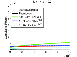
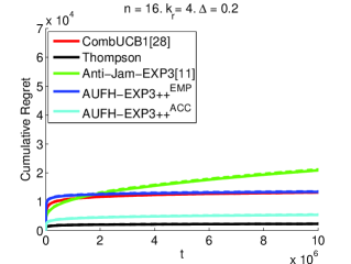
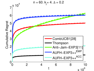
Figure 2: Performance Comparison in the Stochastic Regime.

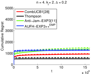
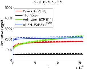
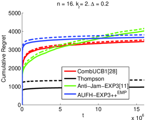
Figure 3: Performance Comparison in the Contaminated Stochastic Regime.

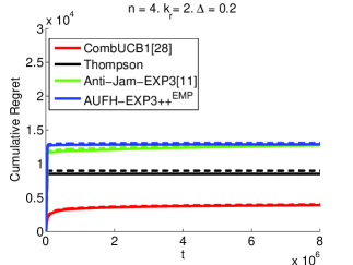
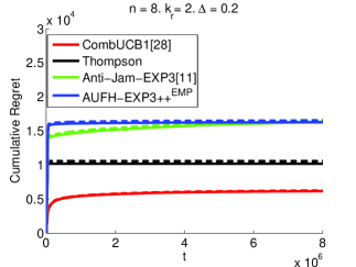
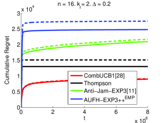
Figure 4: Performance Comparison in the Oblivious Adversarial Regime.

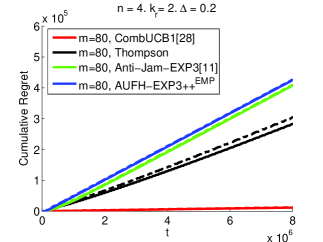
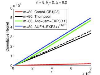
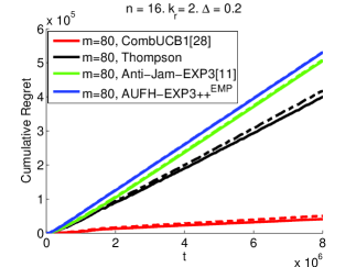
Figure 5: Performance Comparison in the Adaptive Adversarial Regime.

VIII Implementation Issues and Simulation Results

In this section, we consider the wireless communications from a transmitter to a receiver that is by default in the stochastic regime with Bernoulli distributions for rewards. W.l.o.g., we assume a constant unitary data packet rate from the transmitter for each channel $k_{t}\subseteq S_{t}$ over every time slot $t$, i.e. $M=1$ packet, where $k_{t}=4$. All experiments were conducted on an off-the-shelf desktop with dual $6$-core Intel i7 CPUs clocked at $2.66$Ghz. For all the suboptimal channels the rewards are Bernoulli with bias $0.5$, and we set a single best channel whose reward is Bernoulli with bias $0.5+\Delta$.

To show the advantages of our AUFH-EXP3++ algorithms, we compare their performance to other existing MAB based algorithms, which includes: the EXP3 based anti-jamming algorithm in [11], and we named it as “Anti-Jam-EXP3”; The combinatorial UCB-based algorithm “CombUCB1” with almost tight regret bound as proved in [29]; the combinatorial version of the Thompson’s sampling algorithm [35]. Here we consider the use of the Thompson’s sampling algorithm for comparison due to its empirically good performance indicated in [30]. We make ten repetitions of each experiment to reduce the performance bias. In Fig. 2-5, the solid lines in the graphs represent the mean performance over the experiments and the dashed lines represent the mean plus on standard deviation (std) over the ten repetitions of the corresponding experiments. Note that, for a given optimal channel access strategy, small regret values indicate the large number of data packets reception.

At first, we run our experiments by choosing different size of available channels $n=8,16,60$. The size of receiving channels and gap is always $k_{r}=4$ and $\Delta=0.2$, respectively. Our first set of experiments shown in Fig. 2, we run each of the algorithm for $10^{7}$ rounds. We choose $(n,k_{r})$ pairs equals to $(8,4),(16,4),(60,4)$ to see how our algorithms perform from a small size of channel access strategy set ($\binom{8}{4}=70$) to a large size of channel access strategy set ($\binom{60}{4}=487635$). For different versions of our AUFH-EXP3++ algorithms, they are parameterized by ${\xi_{t}}(f)=\frac{{\ln(t{{\hat{\Delta}}_{t}}{{(f)}^{2}})}}{{32t{{\hat{\Delta}}_{t}}{{(f)}^{2}}}}$, where ${{{\hat{\Delta}}_{t}}(f)}$ is the empirical estimate of ${{{\Delta}_{t}}(f)}$ defined in (V-B1). The target of our experiment is to demonstrate that in the stochastic regime the exploration parameters are in full control of the performance we run the AUFH-EXP3++ algorithm with two different learning rates. AUFH-EXP3++^EMP corresponds to $\eta_{t}=\beta_{t}$ and AUFH-EXP3++^ACC corresponds to $\eta_{t}=1$. Note that only AUFH-EXP3++^EMP has a performance guarantee in the adversarial regime. For our AUFH-EXP3++ algorithms, we transform the rewards into losses via $\ell_{t}(f)=1-g_{t}(f)$, other algorithms operate directly on the rewards.

From the results presented in Fig. 2, we see that in all the experiments, the performance of AUFH-EXP3++^EMP is almost identical to the performance of CombUCB1. That means our algorithm can attain almost optimal transmission efficiency in stochastic environments, and our algorithm scales well in the large channel access strategy setting. Thus, AUFH-EXP3++^EMP has all advantages of the stochastic MAB algorithms, and has much better performance gain than Anti-Jam-EXP3 [11]. Moreover, unlike CombUCB1 and Thompson’s sampling, AUFH-EXP3++^EMP is secured against a potential adversary during the wireless communications game. In addition, the AUFH-EXP3++^ACC algorithm can be seen as a special teaser to show the algorithm performance in the condition of $\eta_{t}>\beta_{t}$. It performs better than AUFH-EXP3++^EMP, but it does not have the adversarial regime performance guarantee.

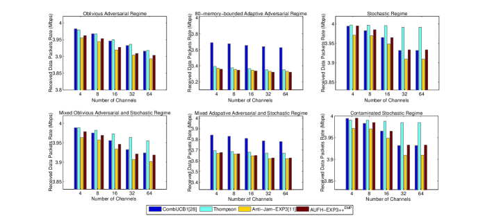
Figure 6: Received Data Packets Rate in Different Regimes. The legend below corresponds to all figures.

In our second set of experiments, we simulate moderately contaminated stochastic environment by drawing the first 2,500 rounds of the game according to one stochastic model and then switching the best channel and continuing the game until $8*10^{6}$ rounds. This action can be regarded as an occasional jamming behavior. In this case, the contamination is not fully adversarial, but drawn from a different stochastic model. We run this experiment with $\Delta=0.2$, $k_{r}=2$ and $n=4,8,16$ to see the noticed leaning performance. The results are presented in Fig. 3. Although it is hard to see the first 2,500 rounds on the plot, their effects on all the algorithms is clearly visible. Despite the initial corrupted rounds the AUFH-EXP3++^EMP algorithm successfully returns to the stochastic operation mode and achieves better results than Anti-Jam-EXP3 [11].

To the best of our knowledge, it is very hard to simulate the fully adversarial regime with arbitrarily changing oblivious jammer. In our third set of experiments shown in Fig. 4, we emulate the adversary regime under oblivious jamming attack by setting the $\Delta$ value of the best channel randomly from $[0.1,0.3]$ and switch the best channel to different indices of channels in the channel set at every other time slot by a pseudorandom sequence generator function. The channel rewards are determined before running the algorithm. It is not difficult to feel that the reward sequences still follow certain stochastic pattern, but not that obvious. We set the typical parameter $k_{r}=2$, $\Delta=0.2$ and run all the algorithms up to $8*10^{6}$ rounds. It can be found that our AUFH-EXP3++^EMP algorithm will be close to and have slightly better performance when compared to Anti-Jam-EXP3 [11], which confirms with our theoretical analysis.

In our fourth set of experiments shown in Fig. 5, we simulate the adaptive jamming attack case in the adversarial regime with a typical memory $m=80$. We can see large performance degradations for all algorithms when compared to the oblivious jammer case. We can find that the performance of AUFH-EXP3++^EMP and Anti-Jam-EXP3 [11] still enjoys the almost the same regret performance, and their large regrets indicate their sensitiveness to the adaptive jammer.

TABLE I: Computation Time Comparisons of Algorithm 1 and Algorithm 2

$(n,k_{r})$
Alg. Ver. vs Comp. Time (micro seconds)	$(12,4)$	$(24,4)$	$(48,6)$	$(48,12)$	$(64,6)$	$(64,12)$	$(64,24)$
AUFH-EXP3++EMP: Algorithm1	23	167	699	2247	8375	162372	862961
AUFH-EXP3++EMP: Algorithm2	4	9	31	57	74	134	280

We also compared the computing time of the two versions of AUFH-EXP3++^EMP, Algorithm 1 and Algorithm 2, with different set of $(n,k_{r})$ pairs for each round. The results are listed in table I. From the results, we can see that Algorithm 2 scales linearly with the increase of the size of $n$ and $k_{r}$, and have very low computational cost than the Algorithm 1. Imagine in a practical typical multi-channel wireless communication system with $(n,k_{r})=(64,12)$, the Algorithm 1 takes about $162$ seconds to finish one round calculation that is infeasible, while the Algorithm 2 takes about $.134$ seconds to finish one round calculation that is very reasonable in practical implementation.

For brevity, we do not plot the regret performance figures for the mixed adversarial and stochastic regime. However, in our last experiments, we compare the received data packets rate (Mbps) for all the four different regimes after a relative long period of learning rounds $t=2*10^{7}$. Here we assume $M=1$ packet contains $1000$ bits and each time slot is just one second. We set $k_{r}=2$ and $\Delta=0.2$ as fixed values for all different size of channel set $n$. We plot our results in Fig. 6. It is easy to find that our algorithm AUFH-EXP3++^EMP attains almost all the advantages of the stochastic MAB algorithms CombUCB1, and has better throughput performance than Anti-Jam-EXP3. As we have noticed, we also put the results of CombUCB1 [29] in the oblivious adversarial, adaptive adversarial and contaminated regimes, etc., although the algorithm is not applicable in theory. This proves that our proposed algorithm AUFH-EXP3++ can be applied for general unknown communication environments in different regimes with flexibility. Interestingly, we find that the Thompson’s sampling algorithm [35] performs superiorly in all regimes, and this empirical fact is observed in the machine learning society. We believe it is a promising direction to study its theoretical ground from the beginning for the collected (security) non–i.i.d. data inputs.

IX Conclusion and Future Works

In this paper, we have proposed the first adaptive multichannel-access algorithm for wireless communications without the knowledge about the nature of environments. At first, we captured the feature of the general wireless environments and divided them into four regimes, and then provided solid theoretical analysis for each of them. Through theoretical analysis, we found that the almost optimal performance is achievable for all regimes. Extensive simulations were conducted to verify the learning performance of our algorithm in different regimes and much better performance improvements over classic approaches. The proposed algorithm could be implemented efficiently in practical wireless communication systems with different sizes. Our framework is of general value, which can be extended by incorporating power control module based on estimated gradient algorithms (under bandit feedback), taking power budgets into account and accessing problems based on observed side information (as “contextual bandit” [1]) for wireless communication scenarios under unexpected security attacks. The idea of this work could also be combined with other online learning-based channel prediction algorithms to perform the joint optimal resource allocation with the configuration of physical layer techniques, such as the MIMO channel and its power allocations. We plan to extend our proposed algorithms to general combinatorial settings and forecast that their variants can be applied in many practical tough environments for wireless networks monitoring, secure routing problems, rumors propagation in social networks (with contextual bandit setting), etc.

Pan Zhou(S’07–M’14) is currently an associate professor with School of Electronic Information and Communications, Huazhong University of Science and Technology, Wuhan, P.R. China. He received his Ph.D. in the School of Electrical and Computer Engineering at the Georgia Institute of Technology (Georgia Tech) in 2011, Atlanta, USA. He received his B.S. degree in the Advanced Class of HUST, and a M.S. degree in the Department of Electronics and Information Engineering from HUST, Wuhan, China, in 2006 and 2008, respectively. He held honorary degree in his bachelor and merit research award of HUST in his master study. He was a senior technical memeber at Oracle Inc, America during 2011 to 2013, Boston, MA, USA, and worked on hadoop and distributed storage system for big data analytics at Oralce cloud Platform. His current research interest includes: communication and information networks, security and privacy, machine learning and big data.

Tao Jiang (M’06–SM’10) is currently a Distinguished Professor in the School of Electronics Information and Communications, Huazhong University of Science and Technology, Wuhan, P. R. China. He received the B.S. and M.S. degrees in applied geophysics from China University of Geosciences, Wuhan, P. R. China, in 1997 and 2000, respectively, and the Ph.D. degree in information and communication engineering from Huazhong University of Science and Technology, Wuhan, P. R. China, in April 2004. From Aug. 2004 to Dec. 2007, he worked in some universities, such as Brunel University and University of Michigan-Dearborn, respectively. He has authored or co-authored over 200 technical papers in major journals and conferences and 8 books/chapters in the areas of communications and networks. He served or is serving as symposium technical program committee membership of some major IEEE conferences, including INFOCOM, GLOBECOM, and ICC, etc.. He is invited to serve as TPC Symposium Chair for the IEEE GLOBECOM 2013, IEEEE WCNC 2013 and ICCC 2013. He is served or serving as associate editor of some technical journals in communications, including in IEEE Transactions on Signal Processing, IEEE Communications Surveys and Tutorials, IEEE Transactions on Vehicular Technology, and IEEE Internet of Things Journal, etc.. He is a recipient of the NSFC for Distinguished Young Scholars Award in 2013, and he is also a recipient of the Young and Middle-Aged Leading Scientists, Engineers and Innovators by the Ministry of Science and Technology of China in 2014. He was awarded as the Most Cited Chinese Researchers in Computer Science announced by Elsevier in 2014. He is a senior member of IEEE.

References

- [1] S. Bubeck and N. Cesa-Bianchi, “Regret Analysis of Stochastic and Nonstochastic Multi-armed Bandit Problems,” Foundation and Trends in Machine Learning, vol. 5, 2012.
- [2] Q. Wang, P. Xu, K. Ren, and M. Li, “Delay-bounded adaptive ufh-based anti-jamming wireless communication,” in Proc. of IEEE INFOCOM 2011, pp. 1413-1421, April, 2011.
- [3] Q. Wang, K. Ren, and P. Ning, “Anti-jamming communication in cognitive radio networks with unknown channel statistics,” in Proc. of IEEE ICNP 2011, pp. 393-402, 2011.
- [4] X. Y. Li, P. Yang, Y. Yan, L. You, S. Tang and Q. Huang, “Almost optimal accessing of nonstochastic channels in cognitive radio networks ,” in Proc. of IEEE INFOCOM 2012, pp. 2291-2299, 2012.
- [5] B. Li, P. Yang, J. Wang, Q. Wu, S. Tang, X.Y. Li, Y. Liu , “Almost Optimal Dynamically-Ordered Channel Sensing and Accessing for Cognitive Networks,” IEEE Transactions on Mobile Computing, pp. 1203-1215, July, 2013.
- [6] Y. Gai and B. Krishnamachari, “Decentralized Online Learning Algorithms for Opportunistic Spectrum Access,” in Proc. of IEEE GLOBECOM 2011, pp. 2534-2539, 2011.
- [7] Y. Zhou, Q. Huang, F. Li, X. Y. Li, M. Liu, Z. Li and Z .Yin, “ Almost Optimal Channel Access in Multi-Hop Networks With Unknown Channel Variables,” in Proc. of IEEE ICDCS 2014, pp. 234-245, 2014.
- [8] Y. Gai, B. Krishnamachari and R. Jain, “Combinatorial Network Optimization with Unknown Variables: Multi-Armed Bandits with Linear Rewards and Individual Observations,” IEEE/ACM Transactions on Networking, vol. 20, no. 5, pp. 1466-1478, 2012.
- [9] R. Zheng, L. Thanh, and H. Zhu, “Approximate online learning for passive monitoring of multi-channel wireless networks,” in Proc. of IEEE INFOCOM 2013, pp. 3111-3119, 2013.
- [10] S. Maghsudi, S. Stnczak, “Joint Channel Selection and Power Control in Infrastructureless Wireless Networks: A Multi-Player Multi-Armed Bandit Framework,” IEEE Transactions on Vehicular Technology, vol. 99, pp. 1-9, 2014.
- [11] Q. Wang, P. Xu, K. Ren, and X. Y. Li, “ Towards optimal adaptive UFH-based anti-jamming wireless communication,” IEEE Journal on Selected Areas in Communications, vol. 99, no.1, pp. 16-30, 2012.
- [12] T. Le, C. Szepesv ri, and R. Zheng, “Sequential Learning for Multi-Channel Wireless Network Monitoring With Channel Switching Costs,” IEEE Transactions on Signal Processing, vol. 62, no. 22, Nov. 15, pp. 1768-1779, 2014.
- [13] A. Anandkumar, N.Michael, and A. K. Tang, “Opportunistic spectrum access withmultiple users: Learning under competition,” in Proc. of IEEE INFOCOM 2010, pp. 803-811, 2010.
- [14] K. Liu, and Q. Zhao, “Online learning for stochastic linear optimization problems,” In proc. of IEEE ITA 2012, pp. 363-367, 2012.
- [15] V. Dani, T. P. Hayes, and S. M. Kakade, “Stochastic Linear Optimization under Bandit Feedback,” In Proc. of COLT 2008, pp. 355-366. 2008.
- [16] R. Arora, D. Ofer, and T. Ambuj, “Online bandit learning against an adaptive adversary: from regret to policy regret,” In Proc. of ICML 2011, pp. 366-377, 2011.
- [17] O. Dekel, G. B. Ran, S. Ohad, and X. Lin, “Optimal distributed online prediction using mini-batches,” In Proc. of ICML 2012, pp. 58-70, 2012.
- [18] T. L. Lai, and H. Robbins, “Asymptotically efficient adaptive allocation rules,” Advances in Applied Mathematics, 6, pp. 23-42, 1985.
- [19] P. Auer, N. Cesa-Bianchi, Y. Freund, and R. E. Schapire, “The nonstochastic multiarmed bandit problem,” SIAM Journal on Computing, vol. 32, no.1, pp.48-77, 2002.
- [20] M. Strasser, C. Ppper, and S. Capkun,“Efficient uncoordinated fhss anti-jamming communication,” in Proc. of ACM MobiHoc 2009, pp.207-218, 2009.
- [21] A. Gyrgy, T. Linder, G. Lugosi, and G. Ottucsk, “The on-line shortest path problem under partial monitoring,” Journal of Machine Learning Research, vol. 8, pp. 2369-2403, 2007.
- [22] N. Cesa-Bianchi, G. Lugosi, “Combinatorial bandits,” Journal of Computer and System Sciences, vol. 78, no.5, pp. 1404-1422, 2012.
- [23] P. Auer, N. Cesa-Bianchi, Y. Freund, and R. E. Schapire, “Gambling in a rigged casino: The adversarial multi-arm bandit problem,” in Proc. of IEEE FOCS’95, pp. 322-331, 1995.
- [24] Y. Seldin, and A. Slivkins, “One practical algorithm for both stochastic and adversarial bandits,” In Proc. of ICML 2014, pp. 358-370, 2014.
- [25] S. Bubeck and A. Slivkins, “The best of both worlds: stochastic and adversarial bandits,” In Proc. of COLT 2012, pp.93-101, 2012.
- [26] A. Mpitziopoulos, D. Gavalas, C. Konstantopoulos, and G. Pantziou, “A Survey on Jamming Attacks and Countermeasures in WSNs,” IEEE Communications Surveys & Tutorials, Vol. 11, Issue No. 4, pp. 42-56, 2009.
- [27] L. Lai, H. E. Gamal, H. Jiang, and H. V. Poor, “Cognitive medium access: Exploration, exploitation and competition,” IEEE Transactions on Mobile Computing, vol. 10, no. 2, pp. 239-253, Feb. 2007.
- [28] K. Liu and Q. Zhao, “Distributed learning in multi-armed bandit with multiple players,” IEEE Transactions on Signal Processing, vol. 58, no. 11, pp. 5667-5681, Nov. 2010.
- [29] B. Kveton, Z. Wen, A. Ashkan, C. Szepesvari, “Tight Regret Bounds for Stochastic Combinatorial Semi-Bandits, in Proc. of AISTATS 2015, pp. 535-543, 2015.
- [30] Y. Seldin, S. Yevgeny, P. Auer, and Y. Abbasi- Yadkori, “ Evaluation and analysis of the performance of the EXP3 algorithm in stochastic environments,” in Proc. of In JMLR EWRL 2013, pp. 145-153, 2013.
- [31] T. He, D. Goeckel, R. Raghavendra, and D. Towsley, “ Endhost-based shortest path routing in dynamic networks: An online learning approach,” In Proc. of IEEE INFOCOM 2013, pp. 2202-2210, 2013.
- [32] A. Jean-Yves, B. Sbastien, L. Gbor, “Regret in Online Combinatorial Optimization,” Mathematics of Operations Research, vo.39, no.1, pp. 31-45, 2014.
- [33] A. G Barto. Reinforcement learning: An introduction. MIT press, 1998.
- [34] P. Auer, N. Cesa-Bianchi, and P. Fischer, “Finite-time analysis of the multiarmed bandit problem,” Machine learning, vol. 47, no. 2-3, pp.235-256, 2002.
- [35] W. R. Thompson, “On the likelihood that one unknown probability exceeds another in view of the evidence of two samples,” Biometrika, vol. 25, pp. 285-294, 1933.