The Carina Project. VIII. The $\alpha$-element abundances. ^,

We have performed a new abundance analysis of Carina red giant (RG) stars from spectroscopic data collected with UVES (high spectral resolution) and FLAMES/GIRAFFE (high and medium resolution) at ESO/VLT. The former sample includes 44 RGs, while the latter consists of 65 (high-resolution) and $\sim$800 (medium-resolution) RGs, covering a significant fraction of the galaxy’s RG branch, and red clump stars. To improve the abundance analysis at the faint magnitude limit, the FLAMES/GIRAFFE data were divided into ten surface gravity and effective temperature bins. The spectra of the stars belonging to the same gravity and temperature bin were stacked. This approach allowed us to increase the signal-to-noise ratio in the faint magnitude limit (V$\geq$20.5 mag) by at least a factor of five. We took advantage of the new photometry index c_U,B,I introduced recently as an age and probably a metallicity indicator to split stars along the red giant branch. These two stellar populations display distinct [Fe/H] and [Mg/H] distributions: their mean iron abundances are –2.15$\pm$0.06 dex ($\sigma$=0.28), and –1.75$\pm$0.03 dex ($\sigma$=0.21), respectively. The two iron distributions differ at the 75% level. This supports preliminary results. Moreover, we found that the old and intermediate-age stellar populations have mean [Mg/H] abundances of –1.91$\pm$0.05 dex ($\sigma$=0.22) and –1.35$\pm$0.03 dex ($\sigma$=0.22); these differ at the 83% level. Carina’s $\alpha$-element abundances agree, within 1$\sigma$, with similar abundances for field halo stars and for cluster (Galactic and Magellanic) stars. The same outcome applies to nearby dwarf spheroidals and ultra-faint dwarf galaxies in the iron range covered by Carina stars. Finally, we found evidence of a clear correlation between Na and O abundances, thus suggesting that Carina’s chemical enrichment history is quite different from that in the globular clusters.

1 Introduction

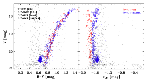
Figure 1: Left: the brighter portion of the CMD of the Carina dwarf in the V vs B–V plane. The large colored circles represent the spectroscopic targets in this investigation. The color coding derives from the selection criteria shown in the right panel. Right: V vs c_U,B,I diagram for the same stars. This particular color combination, (U–B)–(B–I), allows us to split the RGB into old and intermediate-age populations (Monelli et al. 2014).

Empirical evidence indicates that dwarf spheroidal galaxies (dSphs) and ultra-faint dwarfs (UFDs) are the smallest stellar systems to be dominated by dark matter (DM). This finding is supported by new and more precise kinematic measurements (Walker et al. 2009a, b), implying that dSphs and UFDs can provide firm constraints on the smallest DM halos that can retain baryons. The nearby systems have the added advantage that we can sample a significant fraction of their stellar content. Therefore, these interesting stellar systems offer a unique opportunity to simultaneously probe their stellar content and their total mass budget (Walker et al. 2009b).

There is intriguing empirical evidence that both low- and high-mass galaxies follow the stellar mass-metallicity relation (Tinsley & Larson 1979). However, current extragalactic surveys indicate that large galaxies have flat gas-phase metallicity gradients (Moran et al. 2012). Dwarf galaxies, instead, show different peaks in the metallicity distribution (e.g., Tucana, Monelli et al. 2010 and Sculptor, de Boer et al. 2012), but still lack firm evidence of a metallicity gradient (van Zee & Haynes 2006). The available evidence seems to suggest not only that dwarf galaxies appear to be less efficient star formers, but also that their chemical enrichment might have been different from that of massive galaxies.

Cosmological models also suggest that dSphs and UFDs are the fossil records of the Galactic halo (Helmi 2008). Therefore, their kinematic and chemical properties can provide firm constraints on the formation and evolution of the Milky Way (MW). However, recent measurements from high-resolution spectra indicate that the $\alpha$-element abundances in nearby dSphs are, for iron abundances larger than [Fe/H]$>$–2, typically less enhanced than halo stars and Galactic globular clusters where [$\alpha$/Fe]$\approx$0.4 (Tolstoy et al. 2009). This conclusion is supported by a recent investigation based on medium-resolution spectra collected with X-Shooter at VLT for seven either extremely ([Fe/H]$<$–3) or very ([Fe/H]$<$–2) metal-poor stars: Starkenburg et al. (2013) found that the $\alpha$ enhancement is similar in the mean to halo stars of similar metallicities, but the spread around the mean is larger than around the halo stars.

Spectroscopic measurements of metal-poor stars in UFDs support the same scenario, and indeed Gilmore et al. (2013), using high-resolution spectra for seven very metal-poor red giants (RGs) in Boötes I, found that their $\alpha$ enhancement is consistent with halo stars, but showing a spread around the mean.

These findings indicate that the chemical enrichment in low-mass dwarfs has been slower than in the Galactic halo (Cayrel et al. 2004) and in the Galactic bulge (Lagioia et al. 2014). This means that dwarf galaxies might have played a minor role in building up the Galactic spheroid (Leaman et al. 2013; Stetson et al. 2014; Fiorentino et al. 2015).

On the other hand, all the Galactic globular clusters (GCs) investigated so far show a specific chemical fingerprint: the abundances of Na–O and Mg–Al are anticorrelated (Carretta et al. 2009a, b, 2014). This signature becomes even more compelling if we consider the fact that field halo stars do not show evidence of this anticorrelations (Gratton et al. 2000). Moreover, massive GCs with a large spread in iron abundance but a clear evidence of Na–O and Mg–Al anticorrelations ($\omega$-Cen, Johnson et al. 2008; M54, Carretta et al. 2010b) have also been considered relic cores of disrupted dwarf galaxies (Bekki & Freeman 2003). However, the current dwarf galaxies for which we have a detailed knowledge of their chemical enrichment history show a wide range in iron abundance, but no evidence of anticorrelations. This evidence indicates that the role played by GCs and dwarf galaxies in the early formation of the Galactic spheroid is still puzzling.

In this context, the Carina dSph can play a crucial role since it is relatively close (DM₀=20.10 mag, Coppola et al. 2013), it shows at least two clearly separated star-formation episodes, and a wide range in iron that covers at least 1.5 dex. The old stellar population has an age of 12 Gyr, while the intermediate-age has ages ranging from 4 to 8 Gyr (Monelli et al. 2003). In the investigation based on high-resolution (R$\sim$20,000) spectra collected with FLAMES at VLT for 35 RGs, Lemasle et al. (2012) found that the old stellar component in Carina is metal-poor ([Fe/H]$<$–1.5) and slightly $\alpha$-enhanced ([Mg/Fe]$>$0). On the other hand, the intermediate-age population is metal-intermediate (–1.5$<$[Fe/H]$<$–1.2) and shows a broad spread in $\alpha$ enhancement. Indeed, the stars range from being $\alpha$-poor ([Mg/Fe]$<$–0.3) to $\alpha$-enhanced ([Mg/Fe]$\sim$0.3). These findings have been independently supported by the detailed star formation history performed by de Boer et al. (2014). They found evidence of different age-metallicity relations and different trends in the $\alpha$-element distributions between old- and intermediate-age subpopulations. More recently, VandenBerg et al. (2015) used the star formation history provided by de Boer et al. (2014) and found that specific sets of cluster isochrones, covering a broad range in iron and in $\alpha$-element abundances, take account of old horizontal branch (HB) stars and red clump (RC) stars in Carina. It is worth mentioning that these analyses are typically based on stellar ages estimated by comparing the position of the stars in color-magnitude diagrams (CMDs) with specific stellar isochrones. This approach is prone to observational errors in distance determination, photometry, elemental abundances, and interstellar reddening. It is also affected by theoretical uncertainties as the efficiency of diffusive processes, nuclear cross sections, and treatment of superadiabatic convection. For a more detailed discussion of the error budget we refer to Renzini (1991) and Cassisi & Salaris (2013).

A detailed spectroscopic analysis of Carina stars was also performed by Venn et al. (2012) using high-resolution (R$\sim$40,000) spectra for nine bright RGs, collected with UVES at VLT and with MIKE at Magellan. They found evidence of inhomogenous mixing between the old and the intermediate-age population. In particular, a broad spread in Mg was considered suggestive of poor mixing in the gas from which the old population formed, while the offset in $\alpha$-element abundance between the old and the intermediate-age population suggested that the second broader star formation episode in Carina took place in $\alpha$-enriched gas.

The present investigation of the chemical enrichment history of this interesting system is based on the largest homogeneous data set of Carina chemical abundances yet obtained. Our motivation is twofold:
$(i)$ To distinguish old and intermediate-age Carina stars, we use the c_U,B,I=(U–B)–(B–I) index (Monelli et al. 2013, 2014). Detailed photometric investigations indicate that this index can remove the degeneracy between age and metallicity along the red giant branch (RGB). We note that one of the main advantages of this index is that the separation of the two stellar populations relies on a differential measurement. This means that it is independent of uncertainties in the distance modulus, the reddening, and the cluster isochrones.
$(ii)$ We secured high-resolution homogeneous spectra for 44 RGs observed with either UVES or FLAMES/GIRAFFE-UVES with a nominal spectral resolution of 40,000. These spectra were supplemented with high- (R$\sim$20,000) and medium-resolution (R$\sim$6,000) spectra collected with FLAMES/GIRAFFE. Moreover, the latter spectra were also employed to investigate iron and $\alpha$ abundances down to the luminosity of the RC (V$\sim$20.5 mag).

The paper is organized as follows. In Sect. 2 we introduce the photometric index c_U,B,I and its use in separating the old and intermediate-age stellar populations along the Carina RGB. The three spectroscopic data sets adopted in the current investigation are discussed in Sect. 3. In particular, we focus on spectral resolution, wavelength coverage, and the signal-to-noise ratio of the different spectra. In Sect. 4 we describe the procedure adopted to stack the FLAMES/GIRAFFE spectra in detail. This is a fundamental step for providing accurate abundance determinations down to the RC magnitude level. The techniques for measuring equivalent widths, for computing synthetic spectra, and for estimating elemental abundances and their errors are described in Sects. 5 and 6. In these sections we also present a comparison between the current results and those available in the literature. In Sect. 7 we discuss the difference in iron and magnesium abundances between the old and intermediate-age Carina stellar populations. The comparison between Carina’s metallicity distribution and similar abundances in Galactic halo stars and in Galactic and Magellanic globular clusters are discussed in Sects. 8 and 9, respectively. Comparisons between Carina’s $\alpha$-element abundances and similar abundances in dSph and UFD galaxies are presented in Sect. 10. In Sect. 11 we investigate the possibile occurrence of a correlation between Na and O abundances in Carina RGs. Finally, in Sect.12 we summarize the results and outline the future prospects of the Carina Project.

2 c_U,B,I index and different stellar populations

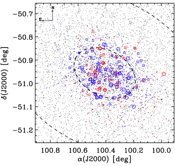
Figure 2: Spatial distribution of our spectroscopic targets. Symbols and colors are the same as in Fig. 1. The dashed ellipses indicate the core and tidal radii of Carina (Mateo 1998).

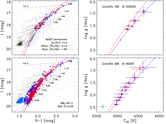
Figure 3: Left column: I vs B–I CMDs showing stars with Giraffe HR (top) or MR (bottom) spectra. Red squares and blue diamonds show the old and intermediate-age stellar components. Dotted lines mark the boundaries of the gravity bins adopted for the spectrum-stacking procedure. Two isochrones from the BaSTI database (Pietrinferni et al. 2004, 2006) are shown as red dashed and blue dot-dashed lines. The adopted distance modulus and reddening are indicated (Coppola et al. 2013). Right column: colored symbols show the positions of the stacked spectra in the stellar parameter $\log g$ vs T_eff plane.

Recent results have revealed that different stellar populations in old Galactic globular clusters can be easily isolated along the whole CMD, from the main sequence, up to the subgiant branch, RGB, and even the HB from an appropriate combination of broadband filters (Marino et al. 2008; Sbordone et al. 2011; Milone et al. 2012). Monelli et al. (2013) showed that their c_U,B,I index is a powerful tool for identifying multiple stellar sequences in the RGB of old GCs, and that the c_U,B,I pseudo-color of RGB stars correlates with the chemical abundances of light elements. Moreover, Monelli et al. (2014) have shown that c_U,B,I can also distinguish a significant fraction of the RGB stars of Carina’s two main populations: the old stars ($\sim$12 Gyr) have a more negative c_U,B,I pseudo-color than the intermediate-age stars (4-8 Gyr).

Figure 1 shows the V vs B–V (left) and V vs c_U,B,I (right) diagrams for stars brighter than V=21 mag: the brighter portion of Carina’s RGB, the RC, and part of the HB, and contaminating field stars at B–V$>$0.45 mag. We note that the main evolutionary features in the V vs c_U,B,I diagram are reversed, and the hottest stars attain higher c_U,B,I values. The distribution of Carina RGB stars in this plane has been discussed by Monelli et al. (2014), who showed that the c_U,B,I index largely removes the age-metallicity degeneracy affecting the RGB stars. Following this analysis, the right panel of Fig. 1 shows a selection of old, more metal-poor (red symbols) and intermediate-age, less metal-poor stars (blue symbols). In particular, the red and blue symbols identify stars with c_U,B,I$<$–1.7 mag and c_U,B,I$>$–1.7 mag, respectively. We note that in the classical V vs B–V plane these stars are mixed along the RGB. The different symbols mark the position of the different spectroscopic data sets (see labels and the discussion in Sect. 3).

The anonymous referee suggested that we discuss in more detail whether the c_U,B,I index is either an age or a metallicity indicator. The empirical evidence suggests that the c_U,B,I index is mainly an age diagnostics, as has previously been discussed in detail by Monelli et al. (2014). However, we address this question below to further support the empirical framework we are developing concerning Carina stellar populations.

Dating back to the seminal investigation by Smecker-Hane et al. (1996), it became clear that Carina experienced two clearly separated star formation episodes. However, optical and optical to near-infrared CMDs indicate that the two subpopulations overlap along the RGB. The c_U,B,I pseudo-color distribution shows clear evidence of an asymmetric and possibly dichotomous distribution of RGB stars. It is plausible to assume that this distribution is correlated with the difference in age of the two subpopulations. This is the reason why we associated the red and the blue RGB stars with the old- and intermediate-age subpopulations. However, we cannot exclude that the c_U,B,I index is also affected by heavy element abundances. This means that the c_U,B,I distribution might also be affected by a difference in CNO and/or in $\alpha$-element abundances. The main conclusion of this investigation, that is, the presence of two subpopulations that experienced two different chemical enrichment histories, is not affected by the intrinsic parameters affecting the c_U,B,I index.

In passing we note that the cut adopted to split old- and intermediate-age subpopulations was fixed according to the c_U,B,I distribution. It is arbitrary, but quantitative tests indicate that plausible changes in the cut do not affect the conclusions concerning the metallicity distributions of the two main subpopulations.

Finally, we note that the age-metallicity pairs found for individual Carina stars by de Boer et al. (2014) and by Lemasle et al. (2012) cannot be recovered in this analysis. The theoretical reasons that led us to overtake the fit with individual cluster isochrones, and in turn individual age estimates of RGB stars, have been discussed in Monelli et al. (2014) and in Sect. 1.

3 Observations and data analyses

Our data were collected with two spectrographs mounted at the UT2 (Kueyen) at the Very Large Telescope (VLT) of the European Southern Observatory (ESO). The Fibre Large Array Multi Element Spectrograph (FLAMES; Pasquini et al. 2002) multi-object spectrograph was used to collect high- and medium-resolution spectra with both the Ultraviolet and Visual Echelle Spectrograph (UVES; Dekker et al. 2000) and GIRAFFE fiber modes. Moreover, we also included in our analysis spectra collected with the slit-mode of UVES.

3.1 UVES and FLAMES/UVES spectra

We present an extension of the analysis for the high-resolution (R$\sim$40,000) UVES and FLAMES/UVES red-arm spectra presented in Fabrizio et al. (2012, Paper V), where we obtained the Fe I and Fe II abundances of 44 red giant Carina stars (hereafter UVES). The stars in Fig. 1 represent the UVES targets (five stars), while the circles are for stars observed with FLAMES/UVES (39 stars). The numbers in parentheses indicate the number of stars belonging to the old (2+8) and intermediate-age (3+31) populations, respectively, based on the c_U,B,I index. Figure 2 shows the spatial distribution of our spectroscopic targets with the same color coding and symbols. The data reduction, radial velocity (RV) measurements, and estimation of the stellar parameters of these spectra follow the approach described in Paper V. In particular, the spectroscopic targets used in this analysis, with photometric, astrometric, and stellar parameters, are listed in Table 1 of Paper V.

3.2 FLAMES/GIRAFFE spectra

To increase the spectroscopic data set and cover the whole extent of the RGB up to the intermediate-age RC helium-burning region (V$\sim$20.5 and B–V$\sim$0.6 mag), we included in our analysis spectra collected with FLAMES/GIRAFFE. In particular, we adopted both the high- (HR10, HR13, and HR14A) and the medium-resolution (LR08) spectra that were presented by Koch et al. (2006), Lemasle et al. (2012), and Fabrizio et al. (2011, Paper IV). The stars with high-resolution spectra were selected using the following criteria: (i) their radial velocities are within 4$\sigma$ from the Carina velocity peak (180$<$RV$<$260 km s^-1) and the precision on the individual RVs is better than 10 km s^-1 (71 stars); (ii) they have been measured in at least three photometric bands (U, B, I); (iii) they have B–I colors that are typical of RGB stars at the same apparent I-band magnitudes ($\Delta$(B–I)$\leq$0.25 mag). We obtained a sample of 65 out of the 71 stars. Almost 50% (35) of the selected stars have previously been analyzed by Lemasle et al. (2012). The others are used here for the first time to estimate iron and $\alpha$-element abundances. We note that selected stars adopted in the stacked spectra have between two to eight individual spectra. We refer to the end of Sect. 4 for a more detailed discussion concerning the number of stars per stacked spectrum.

Similar criteria were also adopted to select 802 stars from the FLAMES/GIRAFFE medium-resolution sample. In particular, we obtained 483 stars along the RGB out of a sample of 529 candidate Carina stars (91%). In the RC region we included 319 stars out of 407 candidate Carina stars (78%). We excluded anomalous Cepheids and bright RC stars. The selected stars, adopted in the stacked spectra, have between two to 35 individual spectra. The reduction of these spectra follows the approach described in Paper IV.

3.2.1 High resolution

The HR spectroscopic targets (hereafter GHR) are shown as colored squares in Figs. 1 and 2. The old population includes 24 stars, while that with intermediate-age stars includes 41 objects. The top left panel of Fig. 3 shows these stars in the I vs B–I CMD (red squares and blue diamonds). Here, we overplotted two isochrones (from the BaSTI database, Pietrinferni et al. 2004, 2006), representing the two main star-formation episodes of Carina. The adopted true distance modulus and reddening values are from Coppola et al. (2013) and are labeled in the figure, and we used extinction coefficients from McCall (2004). The isochrones were used to divide the sample into four bins, using iso-gravity loci (dotted lines). This approach produced four subsamples of spectra that we stacked because they have quite similar stellar parameters. The stellar parameters of each individual star were determined following the procedure described in Paper V. In Table 1 we list the mean values of effective temperature and surface gravity for each bin with their uncertainties and in Col. 4 the number of individual stars per stacked spectrum. We note that the uncertainties in the different bins are the standard deviations of the individual stellar parameters summed in quadrature. The stacking procedure is described in Sect. 4. The top right panel of Fig. 3 shows the position of stacked spectra in the T_eff vs $\log g$ plane (see also Table 1). The bars indicate the range of stellar parameters covered by individual spectra; they range from $\Delta\hbox{$\log g$}$$\sim$0.1 dex, $\Delta\hbox{T${}_{\mathrm{eff}}$}$$\sim$50 K to $\sim$0.25 dex, $\sim$200 K. The signal-to-noise ratio (S/N) of the individual spectra ranges from $\sim$10 to $\sim$50 for the brightest targets. This data set was also adopted by Lemasle et al. (2012) to investigate the chemical abundances of 35 Carina RG stars. It is worth mentioning that the ranges in $\log g$ and T_eff covered by individual spectra belonging to the same gravity and temperature bin allow us to provide accurate abundance estimates. Indeed, the quoted variations in T_eff and $\log g$ (see Sect. 6.4) cause an uncertainty on individual abundances of about 0.15 dex.

Table 1: Stellar parameters of stacked spectra.

ID	Teff (K)	$\log g$	N∗
HRold1	4378$\pm$98	0.92$\pm$0.13	4
HRold2	4604$\pm$112	1.33$\pm$0.15	7
HRold3	4738$\pm$80	1.53$\pm$0.11	9
HRold4	4776$\pm$78	1.65$\pm$0.10	4
HRint1	4368$\pm$130	0.96$\pm$0.19	9
HRint2	4580$\pm$92	1.29$\pm$0.13	14
HRint3	4649$\pm$67	1.54$\pm$0.11	7
HRint4	4760$\pm$71	1.66$\pm$0.11	11
LRold1	4459$\pm$129	0.95$\pm$0.15	8
LRold2	4586$\pm$79	1.31$\pm$0.14	15
LRold3	4709$\pm$75	1.52$\pm$0.11	11
LRold4	4786$\pm$100	1.69$\pm$0.11	14
LRold5	4809$\pm$74	1.81$\pm$0.11	20
LRold6	4896$\pm$78	1.97$\pm$0.11	27
LRold7	4926$\pm$64	2.11$\pm$0.11	32
LRold8	4962$\pm$61	2.21$\pm$0.10	18
LRold9	5026$\pm$56	2.39$\pm$0.11	12
LRint1	4390$\pm$189	0.89$\pm$0.21	14
LRint2	4598$\pm$134	1.30$\pm$0.14	19
LRint3	4741$\pm$104	1.53$\pm$0.11	20
LRint4	4824$\pm$93	1.68$\pm$0.11	33
LRint5	4884$\pm$90	1.81$\pm$0.11	61
LRint6	4909$\pm$84	1.97$\pm$0.11	52
LRint7	4963$\pm$91	2.11$\pm$0.11	50
LRint8	5019$\pm$73	2.24$\pm$0.11	52
LRint9	5037$\pm$63	2.40$\pm$0.11	25
LRrc	5354$\pm$68	2.48$\pm$0.10	319

3.2.2 Medium resolution

We repeated the approach described above with the LR08 spectra (hereafter GMR). This data set is the combination of two observing runs in 2003 (GMR03) and 2008 (GMR08). The details of these samples and their combination were discussed in Paper IV. We obtained 157 stars in the old and 645 stars in the intermediate-age population. The bottom left panel of Fig. 3 shows the CMD and iso-gravity loci. The sample was split into nine bins, plus a particular region enclosing the RC stars. The stellar parameters and their uncertainties were estimated following the same approach discussed in Sect. 3.2.1 and listed in Table 1. The S/N of the individual spectra ranges from $\approx$10 to 50 for GMR03 (17$\lesssim$V$\lesssim$20.5 mag) and from $\approx$5 to 15 for GMR08 (18.5$\lesssim$V$\lesssim$20.75 mag). The positions of the stacked spectra in the T_eff vs $\log g$ plane are shown in the bottom right panel of Fig. 3 (see also Table 1), where we obtained values of variations from $\Delta\hbox{$\log g$}$$\sim$0.1 dex, $\Delta\hbox{T${}_{\mathrm{eff}}$}$$\sim$50 K to $\sim$0.25, $\sim$300 K. In this context, it is worth mentioning that the GMR08 sample was previously used to constrain the kinematic properties of Carina stars (Paper IV). However, this is the first time they are used to constrain the elemental abundances of RG stars down to the RC magnitude level.

For clarity in tracing back the identification of adopted spectra and stars, Table 3.2.2 gives in the first three columns the position ($\alpha$, $\delta$) and the current ID, based on Paper V. Columns 4 and 5 give the IDs of the UVES and GHR samples, while Cols. 6 and 7 report the IDs of the GMR03 and GMR08 samples. The star IDs adopted by Venn et al. (2012) are listed in Col. 8. Moreover, in Table 3.2.2 we also list the same information for the individual GHR and GMR spectra adopted in the stacking of different effective temperature and surface gravity bins (see next section).

Table 2: List of cross-identified spectroscopic targets.

$\alpha$ (J2000)	$\delta$ (J2000)	Fabrizio+12	UVES	GHR	GMR03	GMR08	Venn+12
(deg)	(deg)
099.9825	–50.9602	Car13	LG04c_000951	…	…	…	…
100.1285	–50.9876	Car14	LG04b_004260	…	LG04b_004260	…	…
100.1990	–51.1010	Car15	LG04c_000626	…	LG04c_000626	…	…
100.2374	–50.9773	Car16	CC_09869	MKV0825	…	…	…
100.2379	–50.9624	Car17	CC_09400	MKV0780	LG04a_003830	…	…
100.2419	–51.0334	Car18	CC_11388	…	LG04c_006573	…	…
100.2436	–50.8932	Car19	LG04a_001826	…	…	…	Car–612
100.2471	–51.0408	Car20	CC_11560	…	…	…	…
100.2513	–51.0620	Car21	CC_12038	MKV1012	LG04c_006479	…	…
100.2709	–51.0267	Car22	LG04c_000777	…	…	…	…
100.2940	–50.9314	Car23	CC_08447	…	…	…	…
100.3013	–50.9573	Car24	CC_09226	MKV0770	LG04a_003844	…	…
100.3113	–50.8528	Car25	UKV0524	…	LG04a_002065	…	Car–524
100.3145	–51.0211	Car26	CC_11083	…	LG04c_006621	…	…
HRold1
100.1770	–51.0119	…	…	MKV0914	LG04c_004227	…	…
100.3274	–50.8866	…	…	MKV0596	…	…	…
100.4069	–51.0288	Car36	LG04d_006628	MKV0948	…	…	…
100.4417	–50.8502	Car40	CC_06486	MKV0514	…	…	…

4 Stacking procedure for FLAMES/GIRAFFE spectra

The individual spectra belonging to each bin and population were stacked in a two-step procedure. The first fundamental step is estimating the continuum to gain individual normalized spectra. By default, each spectrum is divided into 200 intervals. To properly identify the continuum while avoiding lines, spikes, and contaminants we calculated the biweight mean (Beers et al. 1990) for each interval using the inverse square-root of the signal as the weight. The mean value was augmented by 75% of the dispersion to define the upper envelope of the signal. Then, the 200 local estimates were connected using a running average with a fixed step of 40. The resulting curve is a good approximation of the continuum over the entire spectral range. The resulting normalized spectra can be visually checked and, if the normalization is problematic, the number of intervals and the averaging step can be changed. In the second step we averaged all normalized spectra belonging to the different gravity bins of the two populations. To do this, each spectrum was accurately rectified for its radial velocity and then was rebinned with a fixed wavelength step (depending on the resolution). Finally, a biweight mean was applied to each wavelength step, averaging all spectra together. Stacking 4-9 (OLD) and 9-14 (INT) individual targets increased the S/N of the GHR spectra, in particular for the faintest targets in the last bin, by a factor of 3-4. For the GMR data set, stacking 8-32 (OLD) and 14-61 (INT) individual targets increases the S/N by a factor of 4-8 (see Table 1). Figure 4 shows an example of the stacked spectrum for an old and an intermediate-age star in the HR10 (top) and LR08 (bottom) grisms. The shaded area represents the dispersion of the individual spectra, and the plots are centered on two Fe I lines that are recognizable in the wavelength range.

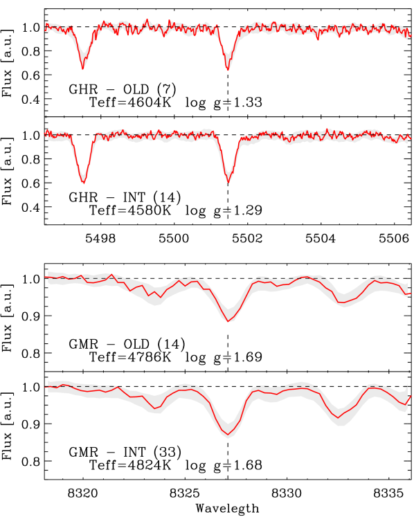
Figure 4: Examples of stacked spectra. Top: resulting stack of 7(14) spectra belonging to the old (intermediate) stellar population, collected with the Giraffe HR10 grism. The shaded area shows the dispersion of individual spectra. We show a portion around an Fe I line marked by the dashed line. Bottom: the same as the top panel, but for spectra collected with Giraffe LR08 grism.

5 Equivalent width measurement

5.1 Line list and atomic data

We selected isolated and unblended iron, sodium, and $\alpha$-element (O I, Mg I, Si I, Ca I, and Ti II) atomic lines in the wavelength range of our spectra from different sources in the literature. In particular, we merged the line lists of Shetrone et al. (2003), Koch et al. (2008a), Fabrizio et al. (2012), Lemasle et al. (2012), and Venn et al. (2012). We updated the atomic data for these lines from the VALD data base (Kupka et al. 2000). The final line lists adopted for each data set are shown in the first four columns of Tables 5.1, 5.1, 5.1, and 5.1. They list the line wavelength (Col.1), element species (Col.2), excitation potential (Col.3), and $\log gf$ (Col.4).

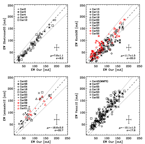
Figure 5: Equivalent width comparisons for stars in common with literature data sets: Shetrone et al. (2003) (top left), Koch et al. (2008a) (top right), Lemasle et al. (2012) (bottom left) and Venn et al. (2012) (bottom right). The dashed line shows the bisector of the plane. The dotted lines display the 10% uncertainty convolved with a 10 mÅ error. The mean measurement errors are also displayed.

Table 3: Equivalent widths (in mÅ) and their errors ($\epsilon$EW) for individual UVES stars.

Table 4: Equivalent widths (in mÅ) and their errors ($\epsilon$EW) for stacked stars in Giraffe HR grisms.

$\lambda$ (Å)	Elem.	$\chi$ (eV)	$\log gf$	HRold1	HRold2	HRold3	HRold4	HRint1	HRint2 …
Giraffe HR10
5339.929	Fe I	3.266	–0.647	…	81.7$\pm$13.4	98.2$\pm$14.2	99.5$\pm$17.4	121.2$\pm$15.0	128.1$\pm$16.7
5341.024	Fe I	1.608	–1.953	161.8$\pm$19.3	122.8$\pm$16.7	113.6$\pm$14.7	95.7$\pm$15.3	205.7$\pm$23.3	156.9$\pm$18.5
5367.466	Fe I	4.415	0.443	63.0$\pm$10.5	71.0$\pm$13.0	73.4$\pm$11.3	…	90.8$\pm$15.1	74.4$\pm$12.8
5383.369	Fe I	4.312	0.645	75.0$\pm$10.2	71.6$\pm$10.2	57.9$\pm$9.0	92.9$\pm$15.5	113.7$\pm$13.3	113.4$\pm$13.4
5393.167	Fe I	3.241	–0.715	88.9$\pm$11.8	86.7$\pm$12.2	74.5$\pm$11.0	71.2$\pm$12.6	124.4$\pm$16.8	105.7$\pm$14.6
5397.128	Fe I	0.915	–1.993	178.8$\pm$21.2	174.1$\pm$20.7	168.3$\pm$21.0	165.2$\pm$22.7	226.0$\pm$26.2	192.9$\pm$22.9
5410.910	Fe I	4.473	0.398	60.6$\pm$9.0	52.8$\pm$8.9	…	…	80.6$\pm$10.0	77.1$\pm$10.2
5429.696	Fe I	0.958	–1.879	199.0$\pm$22.7	179.4$\pm$21.3	188.6$\pm$22.7	156.6$\pm$20.8	251.6$\pm$27.9	226.6$\pm$25.2
5434.524	Fe I	1.011	–2.122	189.0$\pm$22.1	170.1$\pm$20.4	167.7$\pm$20.5	178.7$\pm$24.4	203.9$\pm$24.5	180.3$\pm$21.3
5446.916	Fe I	0.990	–1.914	200.5$\pm$22.6	199.9$\pm$23.0	174.5$\pm$21.0	…	261.3$\pm$28.4	217.8$\pm$24.1
5455.609	Fe I	1.011	–2.091	225.6$\pm$25.2	198.8$\pm$23.0	188.3$\pm$21.9	191.9$\pm$24.5	286.9$\pm$30.3	244.5$\pm$26.2
5501.465	Fe I	0.958	–3.047	135.3$\pm$15.7	115.1$\pm$13.9	103.4$\pm$13.7	106.4$\pm$15.4	170.4$\pm$19.0	142.1$\pm$16.2
5506.779	Fe I	0.990	–2.797	149.4$\pm$17.1	123.4$\pm$14.7	129.6$\pm$16.1	133.9$\pm$18.1	175.9$\pm$19.8	148.3$\pm$16.9
5528.405	Mg I	4.346	–0.620	117.5$\pm$14.4	95.7$\pm$12.1	100.5$\pm$13.0	116.2$\pm$16.0	147.4$\pm$16.5	136.7$\pm$15.7
5581.965	Ca I	2.523	–0.555	41.9$\pm$7.1	…	56.0$\pm$9.5	62.1$\pm$11.6	82.0$\pm$10.1	66.4$\pm$8.7

Giraffe HR13

6122.217 Ca I 1.886 –0.316 110.7$\pm$12.7 111.1$\pm$13.3 81.4$\pm$10.5 …155.7$\pm$16.9 137.0$\pm$15.4 6137.691 Fe I 2.588 –1.403 112.9$\pm$13.3 101.6$\pm$13.3 89.5$\pm$11.8 102.4$\pm$16.8 139.7$\pm$15.5 120.5$\pm$13.9 6161.297 Ca I 2.523 –1.266 ……18.1$\pm$4.2 …41.8$\pm$5.7 30.9$\pm$5.0 6162.173 Ca I 1.899 –0.090 126.5$\pm$14.6 108.4$\pm$13.3 102.5$\pm$12.9 …169.2$\pm$20.0 154.7$\pm$18.1 6166.439 Ca I 2.521 –1.142 …………50.8$\pm$9.8 42.8$\pm$7.4 6213.430 Fe I 2.223 –2.482 62.7$\pm$8.0 63.4$\pm$8.7 45.6$\pm$7.0 73.7$\pm$11.5 111.2$\pm$12.5 89.1$\pm$10.5 6219.281 Fe I 2.198 –2.433 72.9$\pm$9.2 71.5$\pm$9.7 54.8$\pm$8.2 53.9$\pm$9.4 114.8$\pm$13.0 101.8$\pm$11.8 6230.722 Fe I 2.559 –1.281 108.5$\pm$12.9 135.4$\pm$16.7 95.3$\pm$12.4 102.2$\pm$14.8 162.0$\pm$17.9 143.1$\pm$16.7 6252.555 Fe I 2.404 –1.687 109.0$\pm$13.0 96.6$\pm$12.2 85.3$\pm$11.5 109.7$\pm$16.2 143.0$\pm$16.5 121.0$\pm$14.2 6254.258 Fe I 2.279 –2.443 71.0$\pm$9.5 …44.0$\pm$7.7 …117.3$\pm$14.2 101.8$\pm$12.8 6256.361 Fe I 2.453 –2.408 62.0$\pm$8.8 56.4$\pm$8.1 ……107.3$\pm$14.0 91.2$\pm$12.8 6270.223 Fe I 2.858 –2.464 15.7$\pm$3.2 ………52.6$\pm$6.8 36.3$\pm$5.5 6318.018 Fe I 2.453 –2.261 85.5$\pm$11.3 86.7$\pm$11.8 56.6$\pm$8.5 70.4$\pm$11.2 121.5$\pm$14.1 100.6$\pm$12.4 6322.685 Fe I 2.588 –2.426 42.7$\pm$6.2 46.1$\pm$7.5 15.5$\pm$3.9 …83.1$\pm$9.7 56.9$\pm$7.5 6335.330 Fe I 2.198 –2.177 86.4$\pm$10.5 ……100.3$\pm$15.8 126.3$\pm$14.0 112.7$\pm$13.2 6336.823 Fe I 3.686 –0.856 47.3$\pm$6.7 49.8$\pm$8.0 51.2$\pm$8.3 69.4$\pm$13.1 84.5$\pm$10.2 73.4$\pm$9.3    Giraffe HR14    6393.600 Fe I 2.433 –1.432 100.0$\pm$12.0 124.2$\pm$15.3 96.2$\pm$12.8 …146.4$\pm$16.2 135.9$\pm$15.5 6411.648 Fe I 3.654 –0.595 57.3$\pm$7.6 65.8$\pm$9.5 70.4$\pm$10.3 96.0$\pm$15.9 108.6$\pm$12.3 90.3$\pm$10.8 6430.845 Fe I 2.176 –2.006 112.1$\pm$13.3 99.7$\pm$12.5 97.6$\pm$13.6 84.0$\pm$12.9 150.0$\pm$16.4 133.6$\pm$15.3 6439.075 Ca I 2.526 0.390 89.6$\pm$11.0 95.7$\pm$11.8 …102.4$\pm$14.9 148.0$\pm$16.2 113.8$\pm$12.9 6494.980 Fe I 2.404 –1.273 122.1$\pm$15.7 128.8$\pm$16.9 105.4$\pm$14.8 125.7$\pm$19.3 165.8$\pm$21.8 137.4$\pm$19.5 6592.913 Fe I 2.727 –1.473 79.6$\pm$9.4 79.6$\pm$9.8 57.0$\pm$8.2 80.6$\pm$12.8 132.1$\pm$14.4 103.1$\pm$11.7 6593.870 Fe I 2.433 –2.422 65.4$\pm$8.1 …43.3$\pm$7.0 …106.7$\pm$11.9 79.6$\pm$9.4

Table 5: Individual abundances ($\log\epsilon$) and errors for old population stacked stars in Giraffe LR08 grism.

Table 6: Individual abundances ($\log\epsilon$) and errors for intermediate-age population stacked stars in Giraffe LR08 grism

5.2 UVES equivalent widths

The elemental abundances for the UVES and FLAMES/UVES spectra were determined from equivalent width (EW) measurements. EWs were measured with a proprietary IDL interactive procedure, based on a Gaussian or Voigt fitting routine. The user controls the continuum placement, the profile of individual lines, and the contribution of the wings to the EW values. Continuum estimation, in particular, is crucial for the robustness of the final results. To minimize any systematic bias in the continuum estimate that is due to the subjectivity of the operator, three of us have independently performed EW measurements on a sample of selected lines (weak and strong, high and low S/N). The internal dispersion is lower than 6 mÅ, and there is no evidence of systematics. We also performed a sanity check on the profile measurement using the IRAF task splot. The differences are within few percent.

We estimated the uncertainties in the equivalent widths (EW_rms) using the formula presented by Cayrel (1988), revisited by Venn et al. (2012): EW_rms=(S/N)^-1×1.5×FWHM×δx, where S/N is the signal-to-noise ratio per pixel, FWHM is the line full width at half-maximum, and $\delta x$ is the pixel size. Following this approach, we adopted a more conservative EW error: ϵEW=EW_rms+0.1×EW. This conservative approach, which we consider robust, gives EW_rms$\approx$2 mÅ for the whole sample with a final error $\epsilon{\rm EW}$$\approx$10 mÅ. Measured EWs with errors are listed in Table 5.1.

To evaluate the precision of our EWs, we compared the measurements of non-iron group lines (listed in Table 5.1) with those available in the literature. Specifically, we compared EWs from Shetrone et al. (2003), Koch et al. (2008a), and Venn et al. (2012), based on UVES and on FLAMES/GIRAFFE-UVES spectra, and from Lemasle et al. (2012), based on FLAMES/GIRAFFE-HR spectra. Figure 5 shows the EW comparison for the four samples, with our measurements always on the x-axis. The top left panel represents the sample of Shetrone et al. (2003), with which we have five stars in common (one symbol per stars). The black dashed line represents equality, and the dotted lines show a 10% error convolved with the 10 mÅ error, following Shetrone et al. (2003). The error bars in the right bottom corner display the mean errors of the two EW measurements. The mean difference and the dispersion are also labeled (in unit of mÅ). The comparison shows that our estimates are higher on average by $\sim$8 mÅ, but the measurements agree well within 10%. We attribute these systematic differences to the continuum normalization, since a typical uncertainty of 10% on the location of the continuum causes a difference of 10% in the EW.

The top right panel of Fig. 5 shows the same comparison for the sample of Koch et al. (2008a) (ten stars). The higher dispersion ($\sim$20 mÅ) is mainly due to the low S/N of these spectra, while the mean difference is about 12 mÅ. Once again, we overestimated the EWs. The bottom left panel shows the comparison for eleven stars in common with the sample of Lemasle et al. (2012). In this case, the systematic difference is larger ($\sim$–19 mÅ), but here our EW estimates are lower. The high dispersion seems to be caused by the different spectral resolution (GHR$\sim$20,000 vs. UVES$\sim$40,000), and the mean error on EWs decreases by almost a factor of two (20.5 vs $\sim$12 mÅ). The bottom right panel shows the comparison with the recent work of Venn et al. (2012) (seven stars, six of them reanalyzed by us). In this case, we obtain a difference of $\sim$–10 mÅ with a dispersion of 18 mÅ, which is mainly due to the modest S/N of these spectra (10-30).

In conclusion, the data plotted in Fig. 5 indicate that the current EWs agree on average with similar estimates available in the literature, within 10-15%.

6 Abundances

6.1 Model atmospheres

The individual model atmospheres come from the interpolation on the MARCS grid (Gustafsson et al. 2008), using a modified version of the interpolation code developed by Masseron (2006). The individual models were computed for the stellar parameters ($\hbox{T${}_{\mathrm{eff}}$},\log g$) listed in Table 1 of Paper V and in Table 1. Moreover, we selected models with spherical geometry, an $\alpha$-enhanced ([$\alpha$/Fe]=+0.4) chemical mixture, a mass value of 1 M_⊙ , and a constant microturbulence velocity ($\xi$=2 km s^-1), as described in Paper V. It is noteworthy that we did not include lines shortward of 4800 Å to avoid any possible continuum scattering effect in this wavelength region (Sobeck et al. 2011).

6.2 UVES abundances

For the abundance determinations, we used the 2010 version of the stellar abundance code MOOG (Sneden 1973), in particular its abfind driver. The abundances presented in the following sub-sections were computed with a 1D LTE analysis. We chose the solar chemical composition from Grevesse et al. (2007) to be consistent with the iron abundances derived in Paper V. The reference values adopted for the individual species and abundance results are listed in Table 7. The anonymous referee suggested to provide more quantitative estimates concerning the upper limits on the abundances of weak lines (O, Na, Si) in metal-poor stars. To constrain the above limits, we performed a series of simulations using synthetic and observed spectra with S/N$\geq$40. We found that we can measure lines with EWs larger than 11 mÅ for stars with iron abundances ranging from [Fe/H]=–1.50 to [Fe/H]=–2.50. The quoted limit implies upper limits in the abundance of the quoted elements of about [Na/Fe]=–0.9$\div$0.2, [O/Fe]=–0.1$\div$0.6 and [Si/Fe]=–0.6$\div$0.4. We performed the same test using spectra with lower S/N and found that we can only measure lines with EWs larger than 20 mÅ. This means upper limits in the abundances of [Na/Fe]=–0.3$\div$0.8, [O/Fe]=0.2$\div$0.9 and [Si/Fe]=–0.3$\div$0.7.

6.2.1 Comparison with literature values

Figure 6 shows the individual UVES abundance results obtained in this work compared to literature values (rescaled to the same solar reference abundances). In particular, each panel of Fig. 6 shows the $\Delta\hbox{[X/H]}$=[X/H]_UVES–[X/H]_Other as a function of [Fe/H]  for the stars in common with Shetrone et al. (2003, black circles), Koch et al. (2008a, blue squares), Venn et al. (2012, red diamonds), and Lemasle et al. (2012, green triangles). The error bars plotted in this figure were estimated by summing in quadrature current uncertainties with uncertainties evaluated by the quoted authors. The current abundances agree, within 1$\sigma$, with high-resolution abundances available in the literature, namely Shetrone et al. (2003), Venn et al. (2012), and Lemasle et al. (2012). The abundances by Koch et al. (2008a) show a systematic offset and a large scatter when compared with our measurements. The quoted discrepancy appears to be caused by the differences in the measured EWs (see Sect. 5.2 and also Fig. 5) and in the adopted stellar parameters. Their surface gravities are higher on average by 0.5 dex than current ones. The difference seems to be due to the different approach adopted to estimate the gravity, that is, by forcing the balance between Fe I and Fe II vs. photometric gravities. A more detailed discussion is reported in Sect. 5.2 of Paper V. Owing to the lack of evident trends and significant systematics with the estimates available in the literature, we did not apply any correction to our UVES abundances.

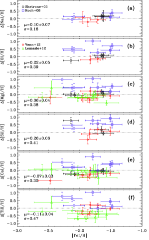
Figure 6: Comparison of UVES abundances with the literature data samples indicated, $\Delta$[X/H]=[X/H]_UVES–[X/H]_Other.

6.3 FLAMES/GIRAFFE-HR abundances

The approach described in Sects. 5.2 and 6.2 was also used to measure the EWs (see Table 5.1) and obtain chemical abundances for the stacked FLAMES/GIRAFFE-HR spectra (see Table 7). To check the validity of our measurements on the stacked spectra and to avoid any systematics, we performed the same analysis on the individual spectra for the stars in common with the UVES sample. We compare the abundances of Fe I, Ca I and Mg I as functions of [Fe/H] in Fig. 7. The agreement is good, within 1$\sigma$ (see labeled values), for most measurements and without evidence of a drift as a function of [Fe/H].

The bottom panel of Fig. 7 shows that four objects display a difference in Mg I abundance that is larger than 1$\sigma$. In particular, the difference for the most metal-poor (Car40) and the most metal-rich (Car51) is about 2$\sigma$. We double-checked these objects together with Car27 and Car33, located at [Fe/H]$\approx$–2, and we found that they are the faintest targets in the UVES data sample, meaning they have the lowest signal-to-noise ratio. Moreover, the continuum in the region bracketing the only available Mg line ($\approx$5528 Å) is relatively noisy. The EWs based on UVES data show a mean difference of $\sim$50 mÅ with those based on HR spectra. We note that these differences do not affect the results of this investigation.

6.4 Abundance uncertainties

The abundance errors were estimated as the maximum of two values. The first comes from propagation of the errors in the EW measurements ($\epsilon$EW), estimated following the approach described in Sect. 5.2, to obtain a $\sigma$(EW) for each line. When the quoted error was asymmetric, the average value was adopted. The second error value was based on the standard deviation of the abundances if more than three lines of the element were available $\sigma(X)$. Otherwise, we set $\sigma(X)$=$\sigma(\hbox{Fe\,{\scriptsize I}})$. Moreover, to account for the uncertainties in the stellar parameters, we added in quadrature the contributions coming from the following error budget: we computed the abundance variations by changing, one at a time, the temperature ($\pm$75 K), gravity ($\pm$0.2 dex), microturbulence ($\pm$0.25 km s^-1), equivalent width ($\pm$10 mÅ), $\log gf$ ($\pm$0.15), metallicity ($\pm$0.2 dex), and $\alpha$-content ($\pm$0.4 dex). We note that we used generous estimates for the uncertainties in the atmospheric parameters (see Paper V) to include the differences between our set of parameters, models, and atomic data as compared to the literature ones. The estimation was performed on the star Car12, since its effective temperature ($\sim$4400 K) and surface gravity ($\sim$0.80 dex) can be considered representative of the entire sample. The results are listed in Table 7. For the FLAMES/GIRAFFE-HR stacked spectra, the dispersion of individual spectra (see the top panel of Fig. 4) produces an uncertainty in the measured EWs of about 10%. In terms of abundances, this effect results in an uncertainty of $\sim$0.15 dex.

Table 7: Impact of uncertainties on abundances for the representative star Car12.

	$\Delta\hbox{T${}_{\mathrm{eff}}$}$		$\Delta\log g$		$\Delta\xi$		$\Delta$EW		$\Delta\log gf$		$\Delta\hbox{[Fe/H]}$		$\Delta\hbox{[$\alpha$/Fe]}$
	(K)		(dex)		(km s-1)		(mÅ)				(dex)		(dex)
Elem.	$-75$	$+75$	$-0.2$	$+0.2$	$-0.25$	$+0.25$	$-10$	$+10$	$-0.15$	$+0.15$	$-0.2$	$+0.2$	$-0.4$	$<$$\sigma$$>$
Na I	$-0.07$	$+0.07$	$+0.01$	$+0.00$	$+0.01$	$-0.01$	$-0.30$	$+0.00$	$+0.15$	$-0.15$	$+0.02$	$-0.01$	$+0.04$	$+0.27$
O I	$-0.02$	$+0.02$	$-0.08$	$+0.09$	$+0.01$	$-0.01$	$-0.21$	$+0.05$	$+0.15$	$-0.15$	$-0.06$	$+0.07$	$-0.09$	$+0.25$
Mg I	$-0.06$	$+0.07$	$+0.02$	$-0.01$	$+0.10$	$-0.09$	$-0.25$	$+0.03$	$+0.15$	$-0.14$	$+0.02$	$-0.01$	$+0.03$	$+0.26$
Si I	$+0.02$	$+0.01$	$-0.01$	$+0.03$	$+0.02$	$-0.01$	$-0.32$	$+0.11$	$+0.15$	$-0.15$	$-0.01$	$+0.02$	$-0.01$	$+0.28$
Ca I	$-0.10$	$+0.10$	$+0.00$	$+0.01$	$+0.12$	$-0.10$	$-0.14$	$+0.18$	$+0.15$	$-0.15$	$+0.04$	$-0.02$	$+0.04$	$+0.27$
Ti II	$+0.02$	$-0.02$	$-0.07$	$+0.07$	$+0.16$	$-0.14$	$-0.18$	$+0.20$	$+0.15$	$-0.15$	$-0.04$	$+0.04$	$-0.06$	$+0.30$
Fe I	$-0.07$	$+0.09$	$-0.02$	$+0.02$	$+0.05$	$-0.04$	$-0.17$	$+0.15$	$+0.15$	$-0.15$	$+0.01$	$+0.00$	$+0.02$	$+0.24$
Fe II	$+0.08$	$-0.06$	$-0.08$	$+0.08$	$+0.07$	$-0.06$	$-0.18$	$+0.18$	$+0.15$	$-0.15$	$-0.06$	$+0.06$	$-0.09$	$+0.28$

6.5 FLAMES/GIRAFFE-MR abundance

The spectral features in the FLAMES/GIRAFFE-MR data are severely affected by the blending effect that is caused by the medium resolution of the spectra (R$\sim$6,000). Equivalent width measurements are thus not reliable; to distinguish the contribution of the various blends, synthetic spectra need to be computed. For this, we used the synth driver of MOOG. The synthetic spectra were convolved with a Gaussian broadening function to reproduce the low instrumental resolution. We excluded the effect of stellar rotation. The synthetic spectra were computed for various abundances of iron, magnesium, and calcium. Then they were compared, line by line, with the observed spectra. The resulting abundance for each line was measured from the minimum of the residual function. The uncertainties for individual lines were estimated as the sum in quadrature of three contributions: the abundance step adopted in spectral synthesis computations, the error in the quadratic fit used to interpolate the residual function, and the resulting uncertainty in the abundances ($\sim$0.15 dex) that is due to the dispersion of individual spectra (see bottom panel of Fig. 4 and Sect. 6.4). Measured abundances with errors are listed in Tables 5.1 and 5.1. To verify the validity of our measurements on the stacked spectra and to avoid any systematics, we performed the same analysis on the individual spectra for the stars in common with the UVES sample. We compare the abundances of Fe I and Mg I as function of [Fe/H] in Fig. 8. The agreement is good, within 1$\sigma$ (see labeled values), for most measurements and without evidence of a trend as a function of [Fe/H]. Figure 9 shows the comparison between the resulting abundances of Fe I and Mg I from stacked FLAMES/GIRAFFE-HR and -MR spectra. We do not find any significant systematic trends between the two data sets. We note that the two objects that in the bottom panel display a difference of about 2$\sigma$ are once again Car27 and Car33, that is, the faintest tail of UVES targets.

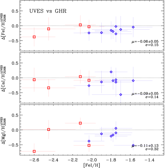
Figure 7: Comparison of Fe I, Ca I, and Mg I abundances between UVES and individual Giraffe HR spectra, $\Delta$[X/H]=[X/H]_UVES–[X/H]_GHR. Red squares and blue diamonds show abundances of old and intermediate-age stars.

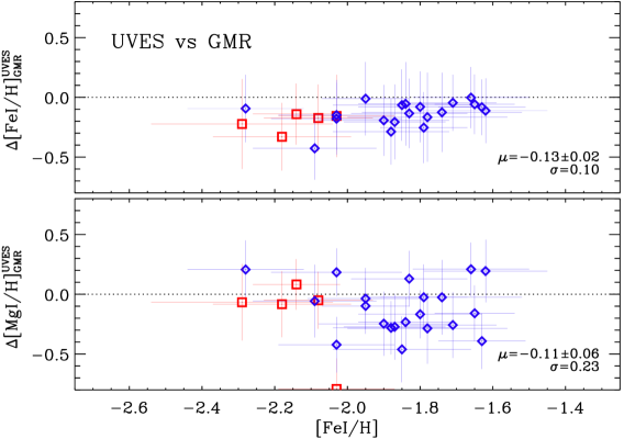
Figure 8: Comparison of Fe Iand Mg I abundances between UVES and individual Giraffe MR spectra, $\Delta$[X/H]=[X/H]_UVES–[X/H]_GMR

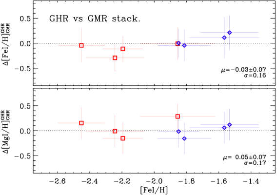
Figure 9: Comparison of Fe I and Mg I abundances between stacked Giraffe HR and LR08 spectra, $\Delta$[X/H]=[X/H]_GHR–[X/H]_GMR

7 Abundances of old and intermediate-age stars

The resulting abundances for individual and stacked spectra are listed in Table 7. Figure 10 shows the Fe I and Mg I abundances as function of gravity for the whole data set. As usual, the red squares are used for the old and the blue diamonds for the intermediate-age population. The plots show an evident dichotomy in the abundances that covers the entire gravity range, from the top of the RGB ($\log g$$\simeq$0.5 dex) to the RC level ($\sim$2.5 dex).

This figure presents several interesting features. (i) Iron abundances (top panel) based on UVES, GHR, and GMR spectra show that the old stellar population is, over the entire gravity range, systematically more metal-poor than the intermediate-age stellar population. The mean iron abundances based on the three different sets of spectra are listed in Table 9. The weighted total mean for the old population is [Fe/H]=–2.15$\pm$0.06 ($\sigma$=0.28), while for the intermediate-age population it is [Fe/H]=–1.75$\pm$0.03 ($\sigma$=0.21). The difference is slightly larger than 1$\sigma$. To provide a more quantitative estimate, we smoothed the metallicity distributions of the old and intermediate-age data sets with a Gaussian kernel with unitary weight and sigma equal to the individual abundance uncertainties. We performed a $\chi^{2}$ comparison of the two distributions and the confidence levels (CL) are listed in Col. 4 of Table 9. These data indicate that the iron abundances of the two stellar populations differ with a confidence level that ranges from 75% (global sample) to 84% (GHR). (ii) Magnesium abundances plotted in the bottom panel of Fig. 10 display a similar trend. The mean abundances for the different spectroscopic samples are also listed in Table 9. The mean magnesium abundance for the old population based on the entire sample is [Mg/H]=–1.91$\pm$0.05 ($\sigma$=0.22), while for the intermediate-age population it is [Mg/H]=–1.35$\pm$0.03 ($\sigma$=0.22). The difference is slightly larger than 1$\sigma$. We followed the same approach adopted for the iron abundances and found that they differ with a confidence level that ranges from 80% (GHR) to 91% (GMR). (iii) The iron and the magnesium abundances based on GHR and GMR spectra agree in the overlapping surface gravity regime, with individual abundances based on UVES spectra. (iv) The largest surface gravity bin ($\log g$=2.48) shows the Fe and the Mg abundances of RC stars. The abundances are, within the errors, similar to the other intermediate-age abundances. This further confirms the difference between the two subpopulations, since RC stars are reliable tracers of the intermediate-age population (Cassisi & Salaris 2013).

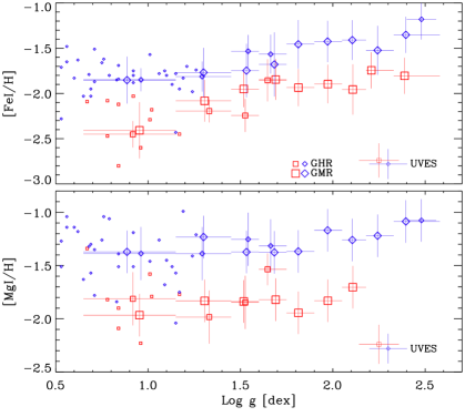
Figure 10: Top: [Fe/H] abundances based on individual and stacked spectra. Red squares and blue diamonds represent abundances of old and intermediate-age stars. Abundances based on individual high-resolution UVES spectra are displayed as small squares and diamonds, without bars. The error bars plotted in the bottom right corner of the panel display the typical uncertainty for the UVES abundances and on surface gravities (see also Paper V). Abundances based on GHR spectra are marked by medium squares and diamonds, while those based on GMR spectra are marked by large squares/diamonds. The vertical bars represent the uncertainty in iron while the horizontal ones show the gravity ranges adopted in Fig. 3. Bottom: same as the top, but for the [Mg/H] abundances.

Table 8: Mean chemical abundances and dispersions of Carina stars.

Car2 0.66$\pm$0.12[1]0.01$\pm$0.24[3]0.45$\pm$0.12[1]…0.35$\pm$0.09[13]0.42$\pm$0.13[7]–1.63$\pm$0.12[17] Car12 0.71$\pm$0.10[2]0.36$\pm$0.35[2]0.58$\pm$0.17[2]0.47$\pm$0.09[3]0.37$\pm$0.20[11]0.58$\pm$0.14[6]–1.62$\pm$0.17[21] Car14 0.46$\pm$0.12[1]…0.47$\pm$0.19[2]0.22$\pm$0.21[2]0.32$\pm$0.10[13]0.48$\pm$0.11[6]–1.79$\pm$0.12[25] Car15 ……0.77$\pm$0.14[2]…0.33$\pm$0.10[11]0.58$\pm$0.19[5]–2.28$\pm$0.16[27] Car16 0.52$\pm$0.17[1]0.33$\pm$0.17[1]0.56$\pm$0.18[2]…0.36$\pm$0.45[14]0.22$\pm$0.34[5]–1.75$\pm$0.17[5]

Table 9: Mean abundances, dispersions and confidence levels (C.L.) for data sets plotted in Fig. 10

. [Fe/H] old [Fe/H] int C.L. [Mg/H] old [Mg/H] int C.L. UVES –2.31$\pm$0.27[10] –1.81$\pm$0.17[34] 82% –2.00$\pm$0.37[10] –1.39$\pm$0.26[32] 82% GHR –2.19$\pm$0.27[4] –1.69$\pm$0.18[4] 84% –1.80$\pm$0.20[4] –1.34$\pm$0.07[4] 80% GMR –1.93$\pm$0.16[9] –1.54$\pm$0.23[10] 75% –1.85$\pm$0.11[7] –1.25$\pm$0.12[10] 91% ALL –2.15$\pm$0.28[23] –1.75$\pm$0.21[48] 75% –1.91$\pm$0.22[21] –1.35$\pm$0.22[46] 83%

8 Comparison with the Galactic halo

Table 10: Comparison of mean abundances and dispersions between Carina, Halo and globular cluster stars.

Elem.	[Fe/H] range	Car. Old	Car. Int.	Carina	MW Halo	MW GCs	LMC GCs
[Na/Fe]	–1.95/–1.48	…	0.18$\pm$0.27[10]	0.18$\pm$0.27[10]	–0.11$\pm$0.29[72]	0.30$\pm$0.29[103]	0.36$\pm$0.32[21]
[O/Fe]	–2.60/–1.48	0.84$\pm$0.27[4]	0.59$\pm$0.19[20]	0.63$\pm$0.23[24]	0.55$\pm$0.33[57]	0.27$\pm$0.15[31]	0.09$\pm$0.15[18]
[Mg/Fe]	–2.80/–1.18	0.29$\pm$0.28[21]	0.40$\pm$0.22[46]	0.36$\pm$0.24[67]	0.34$\pm$0.19[581]	0.27$\pm$0.12[139]	0.09$\pm$0.22[21]
[Si/Fe]	–2.14/–1.48	1.09$\pm$0.12[1]	0.54$\pm$0.22[16]	0.56$\pm$0.25[17]	0.27$\pm$0.25[87]	0.32$\pm$0.10[60]	0.38$\pm$0.15[20]
[Ca/Fe]	–2.80/–1.48	0.18$\pm$0.33[14]	0.27$\pm$0.12[38]	0.25$\pm$0.17[52]	0.20$\pm$0.13[540]	0.23$\pm$0.07[74]	0.21$\pm$0.10[21]
[Ti II/Fe]	–2.80/–1.48	0.40$\pm$0.24[9]	0.24$\pm$0.28[33]	0.28$\pm$0.30[42]	0.34$\pm$0.15[515]	0.35$\pm$0.19[11]	0.53$\pm$0.45[3]
$[$Mg/Ca$]$	–2.80/–1.48	0.13$\pm$0.23[14]	0.15$\pm$0.20[36]	0.15$\pm$0.21[50]	0.03$\pm$0.17[534]	0.03$\pm$0.07[74]	–0.12$\pm$0.29[21]
$\left[\frac{\rm Mg+Ca}{2\rm Fe}\right]$	–2.80/–1.48	0.28$\pm$0.29[14]	0.35$\pm$0.14[36]	0.13$\pm$0.16[50]	0.32$\pm$0.14[533]	0.25$\pm$0.08[71]	0.15$\pm$0.10[21]
$\left[\frac{\rm Mg+Ca+Ti}{3\rm Fe}\right]$	–2.80/–1.48	0.34$\pm$0.30[9]	0.32$\pm$0.17[32]	0.33$\pm$0.19[41]	0.33$\pm$0.13[506]	0.29$\pm$0.12[15]	0.18$\pm$0.09[21]

Figure 11 displays the abundance trends of five $\alpha$-elements, including Na, for the entire sample of old- (red squares) and intermediate-age (blue diamonds) stars. For a detailed comparison with field halo stars, the large sample of elemental abundances compiled by Frebel (2010) is shown as purple dots. These abundances are based on high-resolution spectra of field stars of all evolutionary stages. We note that these measurements have been rescaled to the same solar elemental abundances adopted in this investigation.

The [Na/Fe] abundances are only available for a limited sample (ten) of intermediate-age stars. The mean weighted abundance—[Na/Fe]=0.18 ($\sigma$=0.27)—appears slightly larger than the abundances of field halo stars in the iron range covered by Carina stars—[Na/Fe]=–0.11 ($\sigma$=0.29). However, the difference is within 1$\sigma$ (see Table 10). We note that the field value is based on a large sample (72) and shows an intrinsic dispersion that is higher than the individual measurements (see the error bars plotted in the top right corner). Moreover, intermediate-age Carina stars attain either solar or slightly supersolar Na abundances. The [Na/Fe] abundances provided by Venn et al. (2012) are on average subsolar. The discrepancy for the stars with [Fe/H]$>$–2.0 is caused by the difference in the mean iron abundance $\Delta$(our–Venn)=–0.37$\pm$0.11 dex (see Sect. 5.2 and Fig. 3 in Paper V). In passing we note that the plausibility of the current [Na/H] abundances is supported by the mild difference with similar abundances provided by Shetrone et al. (2003), Venn et al. (2012), and Koch et al. (2008a) (see panel (a) of Fig. 6).

[O/Fe] abundances are available for a few old (four) and for a good sample of intermediate-age (20) stars. They are O enhanced and attain very similar abundances within the errors (see Table 10). The mean weighted [O/Fe] abundance of the entire sample—[O/Fe]=0.63 ($\sigma$=0.23)—agrees quite well with similar abundances—[O/Fe]=0.55 ($\sigma$=0.33)—for field halo stars (57) in the same iron interval. We note that for several metal-poor objects in our sample both O and Si display very weak lines and their EWs have modest or poor precision.

[Mg/Fe] abundances are available for a sizable sample of both old and intermediate-age stars (see Sect. 7). They are Mg enhanced and agree—[Mg/Fe]=0.29 ($\sigma$=0.28) vs [Mg/Fe]=0.40 ($\sigma$=0.22)—within the errors. We note that old and intermediate-age Carina stars show more similar [Mg/Fe] abundances than [Mg/H] because the old sample is systematically more iron-poor than the younger one. The mean weighted [Mg/Fe] abundance of the entire sample—[Mg/Fe]=0.36 ($\sigma$=0.24)—agrees very well with similar abundances—[Mg/Fe]=0.34 ($\sigma$=0.19)—for field halo stars (581) in the same metallicity interval. This finding supports early results obtained by Idiart & Thévenin (2000) concerning the Mg abundances of field Halo stars. The non-LTE correction for the Mg I abundances of both halo and Carina stars were not taken into account. However, Merle et al. (2011) found that the non-LTE corrections to the EWs of two Mg lines at 5711 and 5528 Å are smaller than 10%.

The [Si/Fe] abundances are available for a sizable sample of intermediate-age (16) stars but for only one old star. They are Si enhanced and the mean weighted abundance of the entire sample—[Si/Fe]=0.56 ($\sigma$=0.25)—is larger than the mean abundance—[Si/Fe]=0.27 ($\sigma$=0.25)—of field halo stars (87). They agree within 1$\sigma$. The mean Si abundance decreases to 0.54 dex ($\sigma$=0.22) when the old star is excluded.

The [Ca/Fe] abundances of old (14) and intermediate-age (38) Carina stars agree quite well—[Ca/Fe]=0.18 ($\sigma$=0.33) vs [Ca/Fe]=0.27 ($\sigma$=0.12)—with each other. The weighted mean [Ca/Fe] abundance of the entire sample—[Ca/Fe]=0.25 ($\sigma$=0.17)—agrees very well with similar abundances—[Ca/Fe]=0.20 ($\sigma$=0.13)—for field halo stars (540) in the same iron interval. We excluded the non-LTE corrections to the EWs of Ca I lines for both halo and Carina stars from the comparison. Merle et al. (2011) found that the non-LTE corrections to the EWs of the two adopted Ca I lines (6122, 6166 Å) are smaller than 10%. The anonymous referee noted the paucity of subsolar [Mg/Fe] and [Ca/Fe] abundance ratios, plotted in panels (c) and (e) of Fig. 11, when compared with similar abundances provided by Lemasle et al. (2012). The good agreement between the two different data sets has already been discussed in Sect. 6. The above difference is mainly caused by a difference of –0.27$\pm$0.09 dex in iron abundance. We refer to Paper V for a more detailed discussion.

The [Ti/Fe] abundances are based on Ti II. The abundances of old and intermediate-age Carina stars are enhanced and agree quite well—[Ti/Fe]=0.40 ($\sigma$=0.24) vs [Ti/Fe]=0.24 ($\sigma$=0.28). The former sample includes nine stars, while the latter contains almost three dozen stars. The mean weighted [Ti/Fe] abundance of the entire sample—[Ti/Fe]=0.28 ($\sigma$=0.30)—agrees very well with similar abundances—[Ti/Fe]=0.34 ($\sigma$=0.15)—for field halo stars (515) in the same iron interval. The abundances for neutral Ti I are not used here to avoid non-LTE effects that cause an ionization imbalance in this species, as shown by Bergemann (2011) and Bergemann & Nordlander (2014). It is noteworthy that the correction of $+0.25$ dex for Ti I, suggested by Bergemann (2011) and based on the metal-poor RGB star HD 122563 ([Fe/H]=–2.5), agrees very well with the difference we found in our stars Ti I–Ti II=+0.28 dex.

To further constrain the [$\alpha$/Fe] abundance of Carina stars, we also summed the individual $\alpha$-elements with reliable measurements. The top panel of Fig. 12 shows [Mg+Ca/2Fe] as a function of the iron abundance. The old and the intermediate-age subpopulations have, once again, very similar abundances. They also agree quite well with similar abundances for field halo stars (see also Table 10). The same result is found for the [Mg+Ca+Ti/3Fe] $\alpha$-element abundances plotted in the bottom panel of that figure. The standard deviations of the Carina subpopulations are, as noted by the anonymous referee, larger than the standard deviations of the halo sample. The difference is mainly due to the sample size. We performed a number of tests and found that the Mg distribution of Carina and halo stars agree at 95% CL. We found a similar agreement for the Ca (90% CL) distribution, while for Ti it is at 50% CL. These findings are soundly supported by the mean of the $\alpha$-elements plotted in Fig. 12 and listed in Table 10. The sum of Mg and Ca do agree at 99% CL, while the sum of the three $\alpha$-elements (bottom panel of Fig. 12) agree at 75% CL.

This comparison highlights two relevant findings. (i) The [$\alpha$/Fe] abundances of old and intermediate-age Carina stars are enhanced. They do not show any significant difference within the errors. (ii) The current mean weighted [$\alpha$/Fe] abundances agree quite well with similar abundances of field halo stars in the same range in iron as covered by Carina RG stars.

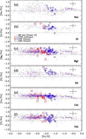
Figure 11: Element abundances as function of [Fe/H]. The open red squares and blue diamonds are the measurements based on UVES spectra of this work for the old and intermediate-age populations. The crossed squares and diamonds show the measurements based on Giraffe-HR spectra, while small solid symbols are for the Giraffe-MR sample. The purple dots show the Milky Way halo stars from Frebel (2010).

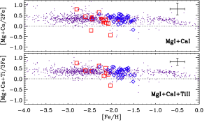
Figure 12: Same as Fig. 11, but for the element combination indicated.

9 Comparison with globular clusters

The comparison between Carina’s elemental abundances and abundances in the Galactic halo is partially hampered by the fact that the latter abundances are derived from spectra with different spectral resolutions and different wavelength ranges. To further constrain the $\alpha$-element abundances of Carina stars, we repeated the comparison using abundances of RG stars in Galactic (Pritzl et al. 2005; Carretta et al. 2009a, b, 2010a) and Magellanic (Mucciarelli et al. 2010; Colucci et al. 2012) globular clusters.

This sample has several distinct differences compared to the field stars: (i) a significant fraction of the abundances rely on high-resolution spectra similar to those of the Carina stars. They also cover very similar wavelength ranges and therefore similar line lists. (ii) A significant fraction of the abundances are on a homogenous $\alpha$-element scale. (iii) The spectroscopic targets include only cluster RG stars. (iv) They show distinctive spectroscopic features (anticorrelations) when compared with field stars, thus suggesting a different chemical enrichment history.

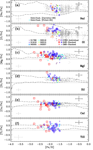
Figure 13: Element abundances as functions of [Fe I/H] for Galactic and some LMC globular clusters. Red squares and blue diamonds show abundances of old and intermediate-age Carina stars. The small cyan asterisks are mean abundances for Galactic globular clusters from Pritzl et al. (2005). The colored small symbols are data for LMC clusters from Mucciarelli et al. (2010, NGC 1786, NGC 2210, and NGC 2257) and Colucci et al. (2012, NGC 1916, NGC 2005, and NGC 2019). The gray dots are individual abundances for 19 Galactic globular clusters from Carretta et al. (2009a, b, 2010a). The gray error bars in the bottom left corner of each panel show the mean abundance errors in GCs. The two dot-dashed lines show the limiting positions of the Milky Way halo stars Frebel (2010).

Panel (a) of Fig. 13 shows that the Na abundances of Carina’s intermediate-age RGs agree quite well with cluster stars. However, Carina RGs, in the metallicity range they cover, attain Na abundances that are slightly underabundant compared to the cluster abundances. They appear, indeed, to agree better with the Na abundances of field halo stars (see Table 10). The two dot-dashed lines plotted in Fig. 13 display the limiting position of Milky Way halo stars according to Frebel (2010). To avoid spurious fluctuations in the range of elemental abundances covered by field stars, we ranked the entire sample as a function of the iron abundance. Then we estimated the running average by using a box including the first 100 objects in the list. We estimated the mean abundances (iron, element) and the standard deviations of the subsample. We estimated the same quantities by moving one object in the ranked list until we took account of the last 100 objects in the sample. We performed several tests changing both the number of objects included in the box and the number of stepping stars. We found that the limiting positions are minimally affected by plausible variations. The comparison between Carina and cluster O abundances is shown in panel (b) of the same figure. Here, the situation is reversed: they attain O abundances that are slightly enhanced compared with cluster stars. The (anti-)correlation Na–O of Carina stars is discussed in more detail in Sect. 11. The Mg abundances of Carina RGs agree quite well with cluster Mg abundances. They show, within the errors, very similar enhancements over the entire metallicity range covered by both globular and Carina samples. The same conclusion applies to globular and Carina Si abundances (see panel (d) of Fig. 13). The comparison between globular and Carina Ca abundances appears to be more complex. Panel (e) of Fig. 13 shows that Carina’s intermediate-age subpopulation agrees quite well with globular Ca abundances. On the other hand, Carina’s old subpopulation shows a slightly broader spread when compared with cluster stars (see Table 10) and with the intermediate-age subpopulation. The internal difference appears reliable ($\sigma$=0.33 vs 0.12 dex), since it is differential and based on GHR and UVES spectra. However, more accurate Ca abundances of Carina old-population stars are required to confirm this preliminary evidence. In passing we note that the current findings support previous results by Thévenin et al. (2001) for Mg and Ca abundances of seven turn-off stars in the metal-poor Galactic globular cluster NGC 6397. The bottom panel of Fig. 13 shows the comparison between globular cluster and Carina Ti II abundances. The two samples agree quite well over the entire metallicity range. There is mild evidence that a fraction of Carina stars might be slightly underabundant in Ti II for [Fe/H]=–1.8, but the difference is within the intrinsic dispersion of the two samples (see error bars).

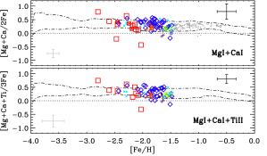
Figure 14: Same as Fig. 13, but for the element combination indicated.

The top and bottom panels of Fig. 14 reveal to even a cursory scrutiny that the sum of Mg and Ca and the sum of Mg, Ca, and Ti II agree quite well with the mean $\alpha$-element abundances of globular stars. This indicates that the $\alpha$-element enrichments appear to be quite similar. This evidence is quite compelling because it applies not only to the old, but also to the intermediate-age subpopulation. In passing we note that this comparison also suggests that nearby stellar systems and field halo stars attain very similar $\alpha$ enhancements in the metallicity range they cover. This further supports the evidence that $\alpha$-elements, in contrast with s- and r-elements, are poor diagnostics to constrain possible differences in chemical enrichment between old and intermediate-age stellar populations (Cescutti 2008; Matteucci et al. 2014).

10 Comparison with nearby dwarfs

Table 11: Mean abundances and dispersions for dSph and UFD galaxies.

Elem.	Draco	Fornax	LeoI	Sculptor	Sextans	UrsaMinor
[Fe I/H]	–2.13$\pm$0.57[15]	–1.27$\pm$0.55[388]	–1.22$\pm$0.20[2]	–2.27$\pm$0.97[17]	–2.53$\pm$0.52[14]	–1.83$\pm$0.30[6]
[Na I/Fe]	–0.19$\pm$0.33[15]	–0.41$\pm$0.28[84]	–0.31$\pm$0.23[2]	–0.15$\pm$0.35[17]	–0.04$\pm$0.28[14]	–0.01$\pm$0.41[6]
[O I/Fe]	0.38$\pm$0.29[11]	0.57$\pm$0.76[3]	0.35$\pm$0.24[2]	0.92$\pm$1.38[11]	0.33$\pm$0.43[7]	0.28$\pm$0.18[6]
[Mg I/Fe]	0.13$\pm$0.26[15]	–0.05$\pm$0.15[201]	–0.06$\pm$0.24[2]	0.19$\pm$0.26[17]	0.09$\pm$0.26[14]	0.30$\pm$0.25[6]
[Si I/Fe]	–0.56$\pm$1.48[13]	–0.03$\pm$0.18[223]	–0.03$\pm$0.22[2]	0.52$\pm$0.91[11]	0.24$\pm$0.22[7]	0.45$\pm$0.37[6]
[Ca I/Fe]	0.05$\pm$0.15[15]	–0.22$\pm$0.13[84]	0.06$\pm$0.21[2]	0.12$\pm$0.27[17]	0.13$\pm$0.16[14]	0.12$\pm$0.16[6]
[Ti II/Fe]	0.39$\pm$0.31[11]	0.14$\pm$0.21[220]	0.25$\pm$0.24[2]	0.18$\pm$0.31[13]	0.09$\pm$0.27[9]	…
Elem.	Boötes	UrsaMaj	ComaBer	Hercules	LeoIV
[Fe I/H]	–2.35$\pm$0.29[7]	–2.89$\pm$0.52[3]	–2.57$\pm$0.30[3]	–2.03$\pm$0.34[2]	–3.14$\pm$0.27[1]
[Na I/Fe]	…	–0.06$\pm$0.09[3]	–0.24$\pm$0.49[3]	0.70$\pm$0.22[2]	0.03$\pm$0.36[1]
[O I/Fe]	…	1.60$\pm$0.94[3]	1.00$\pm$0.55[3]	1.01$\pm$0.24[2]	…
[Mg I/Fe]	0.46$\pm$0.14[7]	0.56$\pm$0.19[3]	0.55$\pm$0.43[3]	0.79$\pm$0.20[2]	0.34$\pm$0.25[1]
[Si I/Fe]	…	1.24$\pm$0.32[3]	0.71$\pm$0.36[3]	0.60$\pm$0.20[2]	…
[Ca I/Fe]	0.26$\pm$0.14[7]	0.37$\pm$0.17[3]	0.45$\pm$0.32[3]	0.03$\pm$0.21[2]	0.23$\pm$0.22[1]
[Ti II/Fe]	…	0.19$\pm$0.05[3]	0.23$\pm$0.23[3]	…	0.38$\pm$0.35[1]

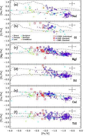
Figure 15: Element abundances as functions of [Fe I/H] for the dwarf spheroidal galaxies (Draco: Shetrone et al. 2001; Fulbright et al. 2004; Cohen & Huang 2009, pluses) - (Fornax: Shetrone et al. 2003; Tafelmeyer et al. 2010; Letarte et al. 2010; Hendricks et al. 2014, circles) - (LeoI : Shetrone et al. 2003, stars) - (Sculptor: Shetrone et al. 2003; Geisler et al. 2005; Frebel et al. 2010a; Starkenburg et al. 2013, triangles) - (Sextans: Shetrone et al. 2001; Aoki et al. 2009; Tafelmeyer et al. 2010, upside-down triangles) - (Ursa Minor: Shetrone et al. 2001, crosses).

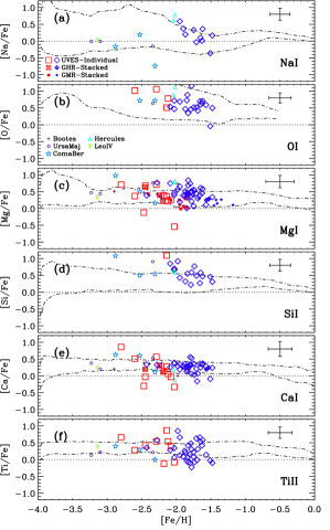
Figure 16: $\alpha$-element abundances as functions of [Fe I/H] for the ultra-faint dwarf galaxies: (Bootes: Feltzing et al. 2009; Norris et al. 2010, pluses) - (Ursa Major: Frebel et al. 2010b, circles) - (ComaBer: Frebel et al. 2010b, stars) - (Hercules: Koch et al. 2008b, triangles) - (LeoIV: Simon et al. 2010, upside-down triangles).

To further characterize the chemical enrichment history of Carina’s old and intermediate-age subpopulations, we extended the comparison to other nearby dSphs and UFDs. The dSphs included in the current comparison—Draco, Fornax, LeoI, Sculptor, Sextans, and Ursa Minor—have accurate elemental abundances from high-resolution spectra, covering a broad range in iron abundances (see Table 11). Moreover, they show quite different star formation histories, but they all host a clearly defined old (t$\sim$12 Gyr) subpopulation. Panels (a) and (b) of Fig. 15 display the comparison between Na and O abundance in Carina and the selected dSphs. These data show that Na and O abundances in nearby dSphs agree within the errors with abundances in field halo stars over the entire metallicity range covered by dSphs. The only exception is Fornax. This is the most metal-rich system and has Na abundances (purple asterisks) that are systematically lower by $\sim$0.3-0.5 dex than field halo stars and the few metal-rich stars in Sculptor (cyan triangles). A similar underabundance in Na was also found by McWilliam et al. (2013) in RGs of the metal-rich Sagittarius dSph galaxy. This is a metallicity regime in which Na abundances might be affected by non-LTE effects (Gratton et al. 1999; Carretta et al. 2010b), but the detailed spectroscopic analysis performed by Fulbright et al. (2007) among K-type giants and FGK-type dwarfs in the Galactic disk indicates that the non-LTE effects are weak (see also McWilliam et al. 2013).

Panels (c), (d), and (e) show the comparison between Mg, Si, and Ca abundances in Carina and other nearby dwarfs. Stars in dSphs are all enhanced in these elements and agree with each other over the entire metallicity range. They also agree quite well with abundances in field Halo stars (dashed lines). The only exception is, once again, Fornax, showing a well-defined underabundance in the quoted $\alpha$ elements. There are a few metal-rich stars in Sculptor showing mild underabundances, but the possible difference is within 1$\sigma$. The bottom panel (f) shows that Ti II abundances in nearby dSphs are on average enhanced over the entire metallicity range. Moreover, they agree quite well with each other and with field Halo stars. The same agreement is also found for Fornax stars. There is weak evidence that the dispersion in Ti II abundances is, at fixed metal content, slightly higher in dwarfs than in the field (see also dispersion values listed in Table 10 and 11).

The insight emerging from this comparisons does not allow us to reach firm conclusions concerning the chemical enrichment history of Carina and nearby dwarfs. Indeed, O, Mg and Na are mainly produced by massive stars during hydrostatic burning phases, and they appear to have similar abundances in nearby dSphs and among field halo stars. On the other hand, the most metal-rich systems (Fornax and Sagittarius) appear to be underabundant in these three elements. The scenario becomes even more surprising for the explosive $\alpha$-elements, namely Si, Ca, and Ti. Si and Ca abundances in field halo stars and in nearby dwarfs, except for Fornax, agree quite well. Once again, metal-rich systems show either solar or slightly underabundant Si and Ca abundances. On the other hand, Ti abundances agree quite well over the entire metallicity range covered by the nearby dSphs.

We performed the same comparisons with RGs in five nearby UFDs (Boötes, Ursa Major, Coma Ber, Hercules, and Leo IV) in Fig. 16. The results are similar to the results found for metal-por dSphs (see Fig. 15 and Table 11). However, the sample of stars is still too limited to reach firm conclusions.

In conclusion, we are left with the following empirical evidence: $\alpha$-element abundances in nearby dwarf are similar to the Galactic field halo stars and to globular clusters in the metal-poor regime ([Fe/H]$<$–1.5). The difference is smaller on average than 1$\sigma$ (see Tables 10 and 11). There is change in the trend when moving into the more metal-rich regime ([Fe/H]$>$–1.5). The Fornax [$\alpha$/Fe] abundance ratios are on average underabundant when compared with halo stars. Sculptor appears to be a transitional stellar system, since the [$\alpha$/Fe] abundance ratios are slightly higher or lower than solar.

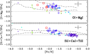
Figure 17: Same as Fig. 15, but for the element combination indicated.

10.1 Hydrostatic vs. explosive

To further investigate the difference between hydrostatic and explosive elements, the top panel of Fig. 17 shows the comparison between the sum of Mg and O for field halo stars. In particular, Mg is produced in hydrostatic core C and O burning, while Ca is one product of explosive Si burning during the supernova type II (SN II) explosion. They overlap quite well until the metal-rich regime. The bottom panel shows the comparison of the sum of the explosive $\alpha$-elements (Si, Ca, and Ti). The agreement is quite good in the metal-poor and in the metal-intermediate iron regimes. The depletion of the quoted sum for Fornax stars in the metal-rich regime is somehow mitigated by the inclusion of titanium. The depletion might have been even stronger if we had only summed Si and Ca abundances of Fornax stars.

Figure 18 shows the comparison between the abundances of two elements, Mg and Ca, as yields of SN II events. The different ratios of these elements are due to the progenitor mass of the SN II (Iwamoto et al. 1999). For Carina, the ratio [Mg/Ca] shows a weaker enhancement than in the MW stars (0.15 vs 0.03 dex, top panel, see also Table 10), but it is well within 1$\sigma$ (0.27 dex). The same behavior is found in the comparison between individual abundances of [Mg/H] and [Ca/H] (bottom panel).

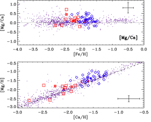
Figure 18: Top panel: the ratio [Mg/Ca] as a function of [Fe/H]for Carina as compared to MW halo stars. Symbols and colors are the same as in Fig. 11. The abundances of [Mg/H] and [Ca/H] are compared in the bottom panel, where the dashed line shows the bisector of the plane.

11 Carina chemical enrichment

Data plotted in Figs. 11 and 12 show that Carina’s chemical enrichment history is quite complex. Similar conclusions were also reached by Lemasle et al. (2012) and Venn et al. (2012), who found evidence that the metal-poor subpopulation is less $\alpha$-enhanced than the metal-rich one. This result was independently supported by de Boer et al. (2014), who performed a detailed star formation history of the Carina dSph galaxy. On the other hand, the current individual (Fig. 11) and mean (Fig. 12) $\alpha$ abundance ratios of the two subpopulations are very similar within 1$\sigma$. Data listed in Table 10 indicate that the difference is at most on the order of 0.1 dex. However, [Mg/Fe] (panel (c) Fig. 11) and [Ca/Fe] (panel (e) Fig. 11) abundance ratios of the old subpopulation appear to be less $\alpha$-enhanced than the intermediate-age subpopulation in the iron range (–2.3$<$[Fe/H]$<$–1.9) they have in common (see also the top panel of Fig. 12). The comparison for the other $\alpha$-elements is hampered by statistics and by the limited range in iron abundance in common between the two subpopulations.

The mean $\alpha$-abundance ratios plotted in the bottom panel of Fig. 12 show that the sum of Mg, Ca, and Ti does not display any significant difference between the old- and the intermediate-age subpopulation. The main difference between the current analysis and previous investigations available in the literature is in the sample size. We worked with $\alpha$-element abundances for 67 stars, 46 of which belonged to the intermediate-age subpopulation. The sample discussed by Lemasle et al. (2012) is a factor of two smaller (35 objects). The difference in the sample size becomes on the order of 20% (55 objects) if we also include abundances on high-resolution spectra provided by Shetrone et al. (2003), Koch et al. (2008a), and Venn et al. (2012).

This evidence indicates that homogeneous $\alpha$-element abundances for a sizable sample of RGB stars do not show a clear difference between old- and intermediate-age subpopulations. The same outcome applies to the possible occurrence of a ”knee” either in the metal-poor ([Fe/H]=–2.5) or in the metal-rich subpopulation ([Fe/H]=–1.6). There are three (Car45, Car27, and Car19) stars in the top panel and two (Car27 and Car19) in the bottom panel of Fig. 12 that show less enhanced $\alpha$ abundance ratios. However, the difference is either within or slightly larger than 1$\sigma$.

To further constrain the chemical enrichment history of Carina, we also investigated the (anti-) correlation between Na and O. There is solid evidence that evolved and unevolved cluster stars display a well-defined anticorrelation in Na–O and in Mg–Al (Carretta et al. 2009a, b, 2014). We note that the environment appears to play a minor role, if any, in these cluster star anticorrelations, and indeed, they have also been identified in globulars belonging to LG dwarf galaxies (LMC, Mucciarelli et al. 2010; Fornax, Letarte et al. 2006).

The occurrence of light-element anticorrelations in GCs is considered to be the consequence of deep potential wells that are able to retain the ejecta of candidate stellar polluters, such as intermediate-mass asymptotic giant branch stars and/or fast-rotating massive stars (see Cassisi & Salaris 2013 and references therein). Nearby dwarf galaxies typically have low central stellar densities (Mateo 1998; McConnachie 2012), therefore a correlation between Na and O is expected. However, we still lack detailed spectroscopic investigations of nearby dSphs that are characterized by high central densities (LeoI, Draco, Ursa Minor). Accurate light element abundances in these systems are required before reaching firm conclusions concerning the environmental impact on their chemical enrichment history.

The top panel of Fig. 19 shows that Carina stars have a (positive) correlation between Na and O. Moreover, the correlation is quite similar to the correlation of field halo stars found by Frebel (2010). The current data soundly support previous results obtained by Carretta et al. (2010b) and McWilliam et al. (2013) for Sagittarius stars. The key advantage of the current comparison is that we investigate the correlation for a system that is significantly more metal-poor than Sagittarius ($\sim-2.0$ vs $\sim-0.6$ dex). To define the difference with cluster stars on a more quantitative basis, the bottom panel shows the comparison between the current sample and the entire sample of cluster stars investigated by Carretta et al. (2009a, b). The difference is quite clear, and indeed Carina stars display a steady increase in the regime of [O/Fe] abundances in which the [Na/Fe] in Galactic globulars becomes less and less abundant. Unfortunately, we cannot constrain whether the candidate old stars show the same trend, since the Na abundance measurements for those stars are lacking.

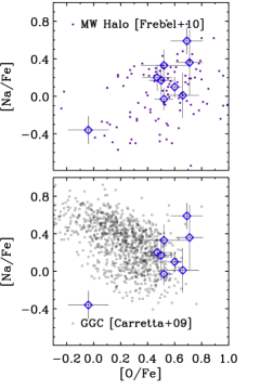
Figure 19: Comparison of Carina stars with MW halo stars (top) and with 1958 stars of 19 galactic globular clusters (bottom, Carretta et al. 2009a, b) in the classical Na vs O diagram.

12 Summary and final remarks

We have presented a new spectroscopic investigation of Carina RG stars. The abundance analysis was focused on Na plus five $\alpha$-elements: O, Mg, Si, Ca, and Ti. The current approach, when compared with similar spectroscopic investigations available in the literature, has two distinct features. (i) We used spectroscopic data collected with UVES (high spectral resolution) and with FLAMES/GIRAFFE (high- and medium-resolution) at the VLT. The current spectroscopic data sets cover a significant fraction of Carina’s RGB and, for the first time, reach the red clump stars (V$\sim$20.5, B–V=0.6 mag), that is, a reliable tracer of the intermediate-age stellar population. We obtained accurate abundance analyses for 44 RGs based on UVES spectra that were previously analyzed in the literature (Koch et al. 2008a; Venn et al. 2012; Fabrizio et al. 2012). They were supplemented with 65 (high-resolution, Lemasle et al. 2012; Fabrizio et al. 2011) and 802 (medium-resolution, Koch et al. 2006; Fabrizio et al. 2011) FLAMES/GIRAFFE spectra. The abundance analysis of 46% of the former sample and 84% of the latter were discussed here for the first time. (ii) We took advantage of the new photometry index c_U,B,I introduced by Monelli et al. (2013, 2014) as an age and probably a metallicity indicator to split stars along the Carina’s RGB. It is noteworthy that the main conclusion of this investigation, that is, the presence of two subpopulations that experienced two different chemical enrichment histories, is not affected by the intrinsic parameters affecting the c_U,B,I index.

To improve the accuracy of the abundance analysis in the faint magnitude limit, we devised a new data reduction strategy. The entire FLAMES/GIRAFFE data set was divided into ten surface gravity and effective temperature bins. The spectra of the stars belonging to the same gravity and temperature bin are characterized by similar stellar parameters and were stacked together. This allowed us to increase the signal-to-noise ratio in the faint magnitude limit (V$\geq$20.5 mag) by at least a factor of five. In this context we note that the spectra of the stars belonging to the same gravity and temperature bin are quite similar because of the modest variation in the intrinsic parameters. This means an improvement in the accuracy of individual abundance estimates. Moreover, this approach allowed us to control possible systematics (surface gravity and effective temperature dependence of non-LTE effects) between the old and intermediate-age stellar populations.

On the basis of these data sets, we have performed the largest and the most homogeneous abundance analysis of the Carina dSph galaxy. The abundances were estimated using both EWs (high-resolution spectra) and spectrum synthesis (medium-resolution stacked spectra).

The main results of the current analysis are listed below. $\bullet$ There is increasing evidence that Carina’s old and intermediate-age stellar populations display two distinct [Fe/H] and [Mg/H] distributions. The dichotomy is present over the entire gravity range (0.5$<$$\log g$$<$2.5); this means from the tip of the RGB down to the RC stars. Specifically, we found that the old stellar populations has a mean iron abundance of –2.15$\pm$0.06 dex ($\sigma$=0.27), while the intermediate-age population has a mean iron abundance of –1.75$\pm$0.03 dex ($\sigma$=0.21). The two distributions differ at the 75% level. This agrees quite well with preliminary results by Monelli et al. (2014) based on data available in the literature and with Lemasle et al. (2012), using a subsample of the current spectroscopic data set. Moreover, we found that the old and intermediate-age stellar populations have mean [Mg/H] abundances of –1.91$\pm$0.05 dex ($\sigma$=0.22) and of –1.35$\pm$0.03 dex ($\sigma$=0.22). They differ at the 83% level. $\bullet$ The individual [$\alpha$/Fe] abundances of Carina’s old and intermediate-age evolved stars are enhanced over the entire iron range. $\bullet$ Carina’s $\alpha$-element abundances and abundances for Galactic halo stars agree quite well (1$\sigma$) over the entire iron range covered by Carina stars. The same conclusion applies to the comparison between $\alpha$-element abundances in Carina and in Galactic and Magellanic globular clusters. However, Na and O abundances display different trends. $\bullet$ Carina’s $\alpha$-element abundances also agree within 1$\sigma$ with similar abundances for LG dwarf spheroidals and ultra-faint dwarf galaxies in the iron range we considered. $\bullet$ We found evidence of a clear correlation between Na and O abundances. Carina’s correlation agrees quite well with the typical Na–O correlation of MW halo stars. This supports previous findings by Carretta et al. (2010b) and McWilliam & Smecker-Hane (2005).

These results support the evidence of a close similarity in the chemical enrichment history of field halo and Carina stars (Idiart & Thévenin 2000).

The stacked spectra will also allow us to investigate the abundances of several s- and r-elements. Of course, the data reduction we devised to stack the spectra in gravity and temperature bins is opening the path to a detailed spectroscopic investigation of the old HB stars (V$\sim$21-21.5 mag), the most reliable tracers of the Carina old stellar population.