Unitarity, Crossing Symmetry and Duality in the scattering of ${\cal N}=1$ Susy Matter Chern-Simons theories

Abstract

We study the most general renormalizable ${\cal N}=1$ $U(N)$ Chern-Simons gauge theory coupled to a single (generically massive) fundamental matter multiplet. At leading order in the $`$t Hooft large $N$ limit we present computations and conjectures for the $2\times 2$ $S$ matrix in these theories; our results apply at all orders in the $`$t Hooft coupling and the matter self interaction. Our $S$ matrices are in perfect agreement with the recently conjectured strong weak coupling self duality of this class of theories. The consistency of our results with unitarity requires a modification of the usual rules of crossing symmetry in precisely the manner anticipated in arXiv:1404.6373, lending substantial support to the conjectures of that paper. In a certain range of coupling constants our $S$ matrices have a pole whose mass vanishes on a self dual codimension one surface in the space of couplings.

1 Introduction

Non-Abelian $U(N)$ gauge theories in three spacetime dimensions are dynamically rich. At low energies parity preserving gauge self interactions are generically governed by the Yang-Mills action

$$\frac{1}{g^{2}_{YM}}\int d^{3}x~{}{\rm Tr}~{}F_{\mu\nu}^{2}\ .$$ (1)

As $g_{YM}^{2}$ has the dimensions of mass, gluons are strongly coupled in the IR. In the absence of parity invariance the gauge field Lagrangian generically includes an additional Chern-Simons term and schematically takes the form

$$\frac{i\kappa}{4\pi}~{}\int~{}{\rm Tr}\left(AdA+\frac{2}{3}A^{3}\right)-\frac{1}{4g^{2}_{YM}}\int d^{3}x~{}{\rm Tr}~{}F_{\mu\nu}^{2}\ .$$ (2)

The Lagrangian (2) describes a system of massive gluons; with mass $m\propto{\kappa g^{2}_{YM}}$. At energies much lower than $g^{2}_{YM}$ (2) has no local degrees of freedom. The effective low energy dynamics is topological, and is governed by the action (2) with the Yang-Mills term set to zero. This so called pure Chern-Simons theory was solved over twenty five years ago by Witten Witten:1988hf ; his beautiful and nontrivial exact solution has had several applications in the study of two dimensional conformal field theories and the mathematical study of knots on three manifolds.

Let us now add matter fields with standard, minimally coupled kinetic terms, (in any representation of the gauge group) to (2). The resulting low energy dynamics is particularly simple in the limit in which all matter masses are parametrically smaller than $g^{2}_{YM}$. In order to focus on this regime we take the limit $g^{2}_{YM}\to\infty$ with masses of matter fields held fixed. In this limit the Yang-Mills term in (2) can be ignored and we obtain a Chern-Simons self coupled gauge theory minimally coupled to matter fields. While the gauge fields are non propagating, they mediate nonlocal interactions between matter fields.

In order to gain intuition for these interactions it is useful to first consider the special case $N=1$, i.e. the case of an Abelian gauge theory interacting with a unit charge scalar field. The gauge equation of motion

$$\kappa\varepsilon^{\mu\nu\rho}F_{\nu\rho}=2\pi J^{\mu}$$ (3)

ensures that each matter particle traps $\frac{1}{\kappa}$ units of flux (where $i\int F=2\pi$ is defined as a single unit of flux). It follows as a consequence of the Aharonov-Bohm effect that exchange of two unit charge particles results in a phase $\frac{\pi}{\kappa}$; in other words the Chern-Simons interactions turns the scalars into anyons with anyonic phase $\pi\nu=\frac{\pi}{\kappa}$.

The interactions induced between matter particles by the exchange of non-abelian Chern-Simons gauge bosons are similar with one additional twist. In close analogy with the discussion of the previous paragraph, the exchange of two scalar matter quanta in representations $R_{1}$ and $R_{2}$ of $U(N)$ results in the phase $\frac{\pi T_{R_{1}}.T_{R_{2}}}{\kappa}$ where $T_{R}$ is the generator of $U(N)$ in the representation $R$. The new element in the non-abelian theory is that the phase obtained upon interchanging two particles is an operator (in $U(N)$ representation space) rather than a number. The eigenvalues of this operator are given by

$$\nu_{R}^{\prime}=\frac{c_{2}(R_{1})+c_{2}(R_{2})-c_{2}(R^{\prime})}{2\kappa}$$ (4)

where $c_{2}(R)$ is the quadratic Casimir of the representation $R$ and $R^{\prime}$ runs over the finite set of representations that appear in the Clebsh-Gordon decomposition of the tensor product of $R_{1}$ and $R_{2}$. In other words the interactions mediated by non-abelian Chern-Simons coupled gauge fields turns matter particles into non-abelian anyons.

In some ways anyons are qualitatively different from either bosons or fermions. For example anyons (with fixed anyonic phases) are never free: there is no limit in which the multi particle anyonic Hilbert space can be regarded as a ‘Fock space’ of a single particle state space. Thus while matter Chern-Simons theories are regular relativistic quantum field theories from a formal viewpoint, it seems possible that they will display dynamical features never before encountered in the study of quantum field theories. This possibility provides one motivation for the intensive study of these theories.

Over the last few years matter Chern-Simons theories have been intensively studied in two different contexts. The ${\cal N}=6$ supersymmetric ABJ and ABJM theories Aharony:2008gk ; Aharony:2008ug have been exhaustively studied from the viewpoint of the AdS/CFT correspondence Maldacena:1997re ; Aharony:1999ti . Several other supersymmetric Chern-Simons theories with ${\cal N}\geq 2$ supersymmetry have also been intensively studied, sometimes motivated by brane constructions in string theory. The technique of supersymmetric localization has been used to perform exact computations of several supersymmetric quantities Drukker:2008zx ; Chen:2008bp ; Bhattacharya:2008bja ; Kim:2009wb ; Kapustin:2009kz ; Marino:2011nm (indices, supersymmetric Wilson loops, three sphere partition functions). These studies have led, in particular, to the conjecture and detailed check for ‘Seiberg like’ Giveon-Kutasov dualities between Chern-Simons matter theories with $\mathcal{N}\geq 2$ supersymmetry Benini:2011mf ; Giveon:2008zn . Most of these impressive studies have, however, focused on observables that are not directly sensitive to the anyonic nature of of the underlying excitations and have exhibited no qualitative surprises.

Qualitative surprises arising from the effectively anyonic nature of the matter particles seem most likely to arise in observables built out of the matter fields themselves rather than gauge invariant composites of these fields. There exists a well defined gauge invariant observable of this sort; the $S$ matrix of the matter fields. While this quantity has been somewhat studied for highly supersymmetric Chern-Simons theories, the results currently available (see e.g. Agarwal:2008pu ; Bargheer:2012cp ; Bianchi:2011fc ; Chen:2011vv ; Bianchi:2011dg ; Bianchi:2014iia ; Bianchi:2012cq ) have all be obtained in perturbation theory. Methods based on supersymmetry have not yet proved powerful enough to obtain results for $S$ matrices at all orders in the coupling constant, even for the maximally supersymmetric ABJ theory. For a very special class of matter Chern-Simons theories, however, it has recently been demonstrated that large $N$ techniques are powerful enough to compute $S$ matrices at all orders in a ‘t Hooft coupling constant, as we now pause to review.

Consider large $N$ Chern-Simons coupled to a finite number of matter fields in the fundamental representation of $U(N)$. It was realized in Giombi:2011kc that the usual large $N$ techniques are roughly as effective in these theories as in vector models even in the absence of supersymmetry (see Aharony:2011jz ; Maldacena:2011jn ; Maldacena:2012sf ; Chang:2012kt ; Aharony:2012nh ; Jain:2012qi ; Yokoyama:2012fa ; GurAri:2012is ; Aharony:2012ns ; Jain:2013py ; Takimi:2013zca ; Jain:2013gza ; Yokoyama:2013pxa ; Bardeen:2014paa ; Jain:2014nza ; Bardeen:2014qua ; Gurucharan:2014cva ; Dandekar:2014era ; Frishman:2014cma ; Moshe:2014bja ; Bedhotiya:2015uga ; Gur-Ari:2015pca for related works). In particular large $N$ techniques have recently been used in Jain:2014nza to compute the $2\rightarrow 2$ $S$ matrices of the matter particles in purely bosonic/fermionic fundamental matter theories coupled to a Chern-Simons gauge field.

Before reviewing the results of Jain:2014nza let us pause to work out the effective anyonic phases for two particle systems of quanta in the fundamental/ antifundamental representations at large $N$. Following Jain:2014nza we refer to any matter quantum that transforms in the (anti)fundamental of $U(N)$ a(n) (anti)particle. A two particle system can couple into two representations $R^{\prime}$ (see (4)); the symmetric representation (two boxes in the first row of the Young Tableaux) and the antisymmetric representation (two boxes in the first column of the Young Tableaux). It is easily verified that the anyonic phase $\nu_{R^{\prime}}$ (see (4)) is of order $\frac{1}{N}$ (and so negligible in the large $N$ limit) for both choices of $R^{\prime}$. On the other hand a particle - antiparticle system can couple into $R^{\prime}$ which is either the adjoint of the singlet. $\nu_{R^{\prime}}$ once again vanishes in the large $N$ limit when $R^{\prime}$ is the adjoint. However when $R^{\prime}$ is the singlet representation it turns out that $\nu_{sing}=\frac{N}{\kappa}=\lambda$ and so is of order unity in the large $N$ limit. In summary two particle systems are always non anyonic in the large $N$ limit of these special theories. Particle - antiparticle systems are also non anyonic in the adjoint channel. However they are effectively anyonic - with an interesting finite anyonic phase- in the singlet channel. See Jain:2014nza for more details. This preparation makes clear that qualitative surprises related to anyonic physics in the two quantum scattering in these theories might occur only in particle - antiparticle scattering in the singlet sector.

The authors of Jain:2014nza used large $N$ techniques to explicitly evaluate the $S$ matrices in all three non-anyonic channels in the theories they studied (see below for more details of this process). They also used a mix of consistency checks and physical arguments involving crossing symmetry to conjecture a formula for the particle - antiparticle $S$ matrix in the singlet channel. The conjecture of Jain:2014nza for the $S$ matrix in the singlet channel has two unexpected novelties related to the anyonic nature of the two particle state

• 1. The singlet $S$ matrix in both the bosonic and fermion theories has a contact term localized on forward scattering. In particular the $S$ matrix is not an analytic function of momenta.

• 2. The analytic part of the singlet $S$ matrix is given by the analytic continuation of the $S$ matrix in any of the other three channels $\times$ $\frac{\sin\pi\lambda}{\pi\lambda}$. In other words the usual rules of crossing symmetry to the anyonic channel are modified by a factor determined by the anyonic phase.

The modification of the usual rules of analyticity and crossing symmetry in the anyonic channel of $2\times 2$ scattering was a major surprise of the analysis of Jain:2014nza . The authors of Jain:2014nza offered physical explanations - involving the anyonic nature of scattering in the singlet channel for both these unusual features of the $S$ matrix. The simple (though non rigorous) explanations proposed in Jain:2014nza are universal in nature; they should apply equally well to all large $N$ Chern-Simons theories coupled to fundamental matter, and not just the particular theories studied in Jain:2014nza . This fact suggests a simple strategy for testing the conjectures of Jain:2014nza which we employ in this paper. We simply redo the $S$ matrix computations of Jain:2014nza in a different class of Chern-Simons theory coupled to fundamental matter and check that the conjectures of Jain:2014nza - unmodified in all details - indeed continue to yield sensible results (i.e. results that pass all necessary consistency checks) in the new system. We now describe the system we study and the nature of our results in much more detail.

The theories we study are the most general power counting renormalizable ${\cal N}=1$ $U(N)$ gauge theories coupled to a single fundamental multiplet (see (2.1) below). In order to study scattering in these theories we imitate the strategy of Jain:2014nza . The authors of Jain:2014nza worked in lightcone gauge; in this paper we work in a supersymmetric generalization of lightcone gauge (3.1). In this gauge (which preserves manifest offshell supersymmetry) the gauge self interaction term vanishes. This fact - together with planarity at large $N$ - allows us to find a manifestly supersymmetric Schwinger-Dyson equation for the exact propagator of the matter supermultiplet. This equation turns out to be easy to solve; the solution gives simple exact expression for the all orders propagator for the matter supermultiplet (see subsection §3.3).

With the exact propagator in hand, we then proceed to write down an exact Schwinger-Dyson equation for the offshell four point function of the matter supermultiplet. The resultant integral equation is quite complicated; as in Jain:2014nza we have been able to solve this equation only in a restricted kinematic range ($q_{\pm}=0$ in the notation of fig 4). In this kinematic regime, however, we have been able to find a completely explicit (if somewhat complicated) solution of the resulting equation(see subsection §3.5-§3.6).

In order to evaluate the $S$ matrices we then proceed to take the onshell limit of our explicit offshell results. As explained in detail in Jain:2014nza , the 3 vector $q^{\mu}$ has the interpretation of momentum transfer for both channels of particle- particle scattering and also for particle antiparticle scattering in the adjoint channel. In these channels the fact that we know the offshell four point amplitudes only when $q_{\pm}=0$ forces us to study scattering in a particular Lorentz frame; any frame in which momentum transfer happens along the spatial $q^{3}$ direction. In any such frame we obtain explicit results for all $2\times 2$ scattering matrices in these three channels. The results are then covariantized to formulae that apply to any frame. Following this method we have obtained explicit results for the $S$ matrices in these three channels. Our results are presented in detail in subsections §3.7 - §3.11. As we explain in detail below, our explicit results have exactly the same interplay with the proposed strong weak coupling self duality of the set of ${\cal N}=1$ Chern-Simons fundamental matter theories (see subsection 2.2) as that described in Jain:2014nza ; duality maps particle - particle $S$ matrices in the symmetric and antisymmetric channels to each other, while it maps the particle - antiparticle $S$ matrix in the adjoint channel to itself.

As in Jain:2014nza our explicit offshell results do not permit a direct computation of the $S$ matrix for particle - antiparticle scattering in the singlet channel. This is because the three vector $q^{\mu}$ is the center of mass momentum for this scattering process and so must be timelike, which is impossible if $q^{\pm}=0$. Our explicit results for the $S$ matrices in the other channels, together with the conjectured modified crossing symmetry rules of Jain:2014nza , however, yield a conjectured formula for the $S$ matrix in this channel.

In section 4 we subject our conjecture for the particle - antiparticle $S$ matrix to a very stringent consistency check; we verify that it obeys the nonlinear unitarity equation (64). From the purely algebraic point of view the fact that our complicated S matrices are unitary appears to be a minor miracle- one that certainly fails very badly for the $S$ matrix obtained using the usual rules of crossing symmetry. We view this result as very strong evidence for the correctness of our formula, and indirectly for the modified crossing symmetry rules of Jain:2014nza .

Our proposed formula for particle - antiparticle scattering in the singlet channel has an interesting analytic structure. As a function of $s$ (at fixed $t$) our $S$ matrix has the expected two particle cut starting at $s=4m^{2}$. In a certain range of interaction parameters it also has poles at smaller (though always positive) values of $s$. These poles represent bound states; when they exist these bound states must be absolutely stable even at large but finite $N$, simply because they are the lightest singlet sector states (baring the vacuum) in the theory; recall that our theory has no gluons. Quite remarkably it turns out that the mass of this bound state supermultiplet vanishes at $w=w_{c}(\lambda)$ where $w$ is the superpotential interaction parameter of our theory (see (2.1)) and $w_{c}(\lambda)$ is the simple function listed in (244). In other words a one parameter tuning of the superpotential is sufficient to produce massless bound states in a theory of massive ‘quarks’; we find this result quite remarkable. Scaling $w$ to $w_{c}$ permits a parametric separation between the mass of this bound state and all other states in the theory. In this limit there must exist a decoupled QFT description of the dynamics of these light states even at large but finite $N$; it seems likely to us that this dynamics is governed by a ${\cal N}=1$ Wilson-Fisher fixed point. We leave the detailed investigation of this suggestion to future work.

The $S$ matrices computed and conjectured in this paper turn out to simplify dramatically at $w=1$, at which point the system (2.1) turns out to enjoy an enhanced ${\cal N}=2$ supersymmetry. In the three non-anyonic channels our $S$ matrix reduces simply to its tree level counterpart at $w=1$. It follows, in other words, that the $S$ matrix is not renormalized as a function of $\lambda$ in these channels. This result illustrates the conflict between naive crossing symmetry and unitarity in a simple setting. Naive crossing symmetry would yield a singlet channel $S$ matrix that is also tree level exact. However tree level $S$ matrices by themselves can never obey the unitarity equations (they do not have the singularities needed to satisfy the Cutkosky’s rules obtained by gluing them together). The resolution to this paradox appears simply to be that the naive crossing symmetry rules are wrong in the current context. Applying the conjectured crossing symmetry rules of Jain:2014nza we find a singlet channel $S$ matrix that continues to be very simple, but is not tree level exact, and in fact satisfies the unitarity equation.

In this paper we have limited our attention to the study of ${\cal N}=1$ theories with a single fundamental matter multiplet. Were we to extend our analysis to theories with two multiplets we would encounter, in particular, the ${\cal N}=3$ theory. Extending to the study of a theory with four multiplets (and allowing for the the gauging of a $U(1)$ global symmetry) would allow us to study the ${\cal N}=6$ $U(N)\times U(1)$ ABJ theory. We believe it would not be difficult to adapt the methods of this paper to find explicit all orders results for the $S$ matrices of all these theories at leading order in large $N$. We expect to find scattering matrices that are unitary precisely because they transform under crossing symmetry in the unusual manner conjectured in Jain:2014nza . It would be particularly interesting to find explicit results for the ${\cal N}=6$ theory in order to facilitate a detailed comparison with the perturbative computations of $S$ matrices in ABJM theory Agarwal:2008pu ; Bargheer:2012cp ; Bianchi:2011fc ; Chen:2011vv ; Bianchi:2011dg ; Bianchi:2014iia ; Bianchi:2012cq , which appear to report results that are crossing symmetric but (at least naively) conflict with unitarity.

2 Review of Background Material

2.1 Renormalizable ${\cal N}=1$ theories with a single fundamental multiplet

In this paper we study $2\times 2$ scattering in the most general renormalizable ${\cal N}=1$ supersymmetric $U(N)$ Chern-Simons theory coupled to a single fundamental matter multiplet. Our theory is defined in superspace by the Euclidean action Avdeev:1992jt ; Ivanov:1991fn

$$\mathcal{S}_{\mathcal{N}=1}=-\int d^{3}xd^{2}\theta\biggl{[}\frac{\kappa}{2\pi}Tr\biggl{(} -\frac{1}{4}D_{\alpha}\Gamma^{\beta}D_{\beta}\Gamma^{\alpha}-\frac{1}{6}D^{\alpha}\Gamma^{\beta}\{\Gamma_{\alpha},\Gamma_{\beta}\}-\frac{1}{24}\{\Gamma^{\alpha},\Gamma^{\beta}\}\{\Gamma_{\alpha},\Gamma_{\beta}\}\biggr{)}$$

$$-\frac{1}{2}(D^{\alpha}\bar{\Phi}+i\bar{\Phi}\Gamma^{\alpha})(D_{\alpha}\Phi-i\Gamma_{\alpha}\Phi)+m_{0}\bar{\Phi}\Phi+\frac{\pi w}{\kappa}(\overline{\Phi}\Phi)^{2}\biggr{]}\ .$$ (5)

The integration in (2.1) is over the three Euclidean spatial coordinates and the two anticommuting spinorial coordinates $\theta^{\alpha}$ (the $SO(3)$ spinorial indices $\alpha$ range over two allowed values $\pm$). The fields $\Phi$ and $\Gamma^{\alpha}$ in (2.1) are, respectively, complex and real superfields . They may be expanded in components as

$$\Phi=\phi+\theta\psi-\theta^{2}F\ ,$$

$$\bar{\Phi}=\bar{\phi}+\theta\bar{\psi}-\theta^{2}\bar{F}\ ,$$

$$\Gamma^{\alpha}=\chi^{\alpha}-\theta^{\alpha}B+i\theta^{\beta}A_{\beta}^{\ \alpha}-\theta^{2}(2\lambda^{\alpha}-i\partial^{\alpha\beta}\chi_{\beta})\ ,$$ (6)

where $\Gamma_{\alpha}$ is an $N\times N$ matrix in color space, while $\Phi$ is an $N$ dimensional column.

The superderivative $D_{\alpha}$ in (2.1) is defined by

$$D_{\alpha}=\frac{\partial}{\partial\theta^{\alpha}}+i\theta^{\beta}\partial_{\alpha\beta}\ ,D^{\alpha}=C^{\alpha\beta}D_{\beta}\ ,$$ (7)

where $C^{\alpha\beta}$ is the charge conjugation matrix. See Appendix §A.1 for notations and conventions.

The theories (2.1) are characterized by one dimensionless coupling constant $w$, a dimensionful mass scale $m_{0}$, and two integers $N$ (the rank of the gauge group $U(N)$) and $\kappa$, the level of the Chern-Simons theory. In the large $N$ limit of interest to us in this paper, the $`$t Hooft coupling $\lambda=\frac{N}{\kappa}$ is a second effectively continuous dimensionless parameter.

The action (2.1) enjoys invariance under the super gauge transformations

$$\delta\Phi=iK\Phi\ ,$$

$$\delta\bar{\Phi}=-i\bar{\Phi}K\ ,$$

$$\delta\Gamma_{\alpha}=D_{\alpha}K+[\Gamma_{\alpha},K]\ ,$$ (8)

where $K$ is a real superfield (it is an $N\times N$ matrix in color space).

(2.1) is manifestly invariant under the two supersymmetry transformations generated by the supercharges $Q_{\alpha}$

$$Q_{\alpha}=i(\frac{\partial}{\partial\theta^{\alpha}}-i\theta^{\beta}\partial_{\beta\alpha})$$ (9)

that act on $\Phi$ and $\Gamma_{\alpha}$ as

$$\delta_{\alpha}\Phi=Q_{\alpha}\Phi\ ,$$

$$\delta_{\alpha}\Gamma_{\beta}=Q_{\alpha}\Gamma_{\beta}\ .$$ (10)

The differential operators $Q_{\alpha}$ and $D_{\alpha}$ obey the algebra

$$\{Q_{\alpha},Q_{\beta}\}=2i\partial_{\alpha\beta}\ ,$$

$$\{D_{\alpha},D_{\beta}\}=2i\partial_{\alpha\beta}\ ,$$

$$\{Q_{\alpha},D_{\beta}\}=0\ .$$ (11)

At the special value $w=1$, the action (2.1) actually has enhanced supersymmetry; it is ${\cal N}=2$ (four supercharges) supersymmetric.

The physical content of the theory (2.1) is most transparent when the Lagrangian is expanded out in component fields in the so called Wess-Zumino gauge - defined by the requirement

$$B=0\ ,\chi=0\ .$$ (12)

Imposing this gauge, integrating over $\theta$ and eliminating auxiliary fields we obtain the component field action

$$\mathcal{S}_{\mathcal{N}=1}=\int d^{3}x\biggl{(} -\frac{\kappa}{2\pi}\epsilon^{\mu\nu\rho}\text{Tr}\big{(}A_{\mu}\partial_{\nu}A_{\rho}-\frac{2i}{3}A_{\mu}A_{\nu}A_{\rho}\big{)}+\mathcal{D}^{\mu}\bar{\phi}\mathcal{D}_{\mu}\phi+m_{0}^{2}\bar{\phi}\phi-\bar{\psi}(i\not{\mathcal{D}}+m_{0})\psi$$

$$+\frac{4\pi wm_{0}}{\kappa}(\bar{\phi}\phi)^{2}+\frac{4\pi^{2}w^{2}}{\kappa^{2}}(\bar{\phi}\phi)^{3}-\frac{2\pi}{\kappa}(1+w)(\bar{\phi}\phi)(\bar{\psi}\psi)-\frac{2\pi w}{\kappa}(\bar{\psi}\phi)(\bar{\phi}\psi)$$

$$+\frac{\pi}{\kappa}(1-w)\big{(}(\bar{\phi}\psi)(\bar{\phi}\psi)+(\bar{\psi}\phi)(\bar{\psi}\phi)\big{)}\biggr{)}$$ (15)

displaying that (2.1) is the action for one fundamental boson and one fundamental fermion coupled to a Chern-Simons gauge field. Supersymmetry sets the masses of the bosonic and fermionic fields equal, and imposes several relations between a priori independent coupling constants.

2.2 Conjectured Duality

It has been conjectured Jain:2013gza that the theory (2.1) enjoys a strong weak coupling self duality. The theory (2.1) with $`$t Hooft coupling $\lambda$ and self coupling parameter $w$ is conjectured to be dual to the theory with $`$t Hooft coupling $\lambda^{\prime}$ and self coupling $w^{\prime}$ where

$$\lambda^{\prime}=\lambda-\text{Sgn}(\lambda)\ ,\ w^{\prime}=\frac{3-w}{1+w}\,~{}~{}~{}m_{0}^{\prime}=\frac{-2m_{0}}{1+w}\ .$$ (16)

As we will explain below, the pole mass for the matter multiplet in this theory is given by

$$m=\frac{2m_{0}}{2+(-1+w)\lambda\ \text{Sgn(m)}}\ .$$ (17)

It is easily verified that under duality

$$m^{\prime}=-m\ .$$ (18)

The concrete prior evidence for this duality is the perfect matching of $S^{2}$ partition functions of the two theories. This match works provided Jain:2013gza

$$\lambda m(m_{0},w)\geq 0\ ,$$ (19)

Through this paper we will assume that (19) is obeyed. Note that the condition (19) is preserved by duality (i.e. a theory and its conjectured dual either both obey or both violate (19)).

Note that $w=1$ is a fixed point for the duality map (16); this was necessary on physical grounds (recall that our theory has enhanced ${\cal N}=2$ supersymmetry only at $w=1$). In the special case $w=1$ and $m_{0}=0$, the duality conjectured in this subsection reduces to the previously studied duality Benini:2011mf (a variation on Giveon- Kutasov duality Giveon:2008zn ). Over the last few years this supersymmetric duality has been subjected to (and has successfully passed) several checks performed with the aid of supersymmetric localization, including the matching of three sphere partition function, superconformal indices and Wilson loops on both sides of the duality Drukker:2008zx ; Chen:2008bp ; Bhattacharya:2008bja ; Kim:2009wb ; Kapustin:2009kz ; Marino:2011nm ; Aharony:2012ns .

2.3 Properties of free solutions of the Dirac equation

In subsequent subsections we will investigate the constraints imposed supersymmetry on the $S$ matrices of the the theory (2.1). Our analysis will make heavy use of the properties of the free solutions to Dirac’s equations, which we review in this subsection.

Let $u_{\alpha}$ and $v_{\alpha}$ are positive and negative energy solutions to Dirac’s equations with mass $m$. Let $p^{\mu}=(\sqrt{m^{2}+{\mathbf{p}}^{2}},{\mathbf{p}})$. Then $u_{\alpha}$ and $v_{\alpha}$ obey

$$({\not{p}}-m)u(p)=0\ ,$$ (20)

$$({\not{p}}+m)v(p)=0\ .$$

We choose to normalize these spinors so that

$$\begin{split}{\bar{u}}({\mathbf{p}})\cdot u({\mathbf{p}})&=-2m~{}~{}~{}~{}~{}~{}~{}~{}~{}~{}~{}~{}~{}~{}~{}{\bar{v}}({\mathbf{p}})\cdot v({\mathbf{p}})=2m\\ u({\mathbf{p}})u^{*}({\mathbf{p}})&=-({\not{p}}+m)C~{}~{}~{}~{}~{}~{}~{}v({\mathbf{p}})v^{*}({\mathbf{p}})=-({\not{p}}-m)C\ .\end{split}$$ (21)

$C$ in (21) is the charge conjugation matrix defined to obey the equation

$$C\gamma^{\mu}C^{-1}=-(\gamma^{\mu})^{T}\ .$$ (22)

Throughout this paper we use $\gamma$ matrices that obey the algebra

$$\{\gamma^{\mu},\gamma^{\nu}\}=-2\eta^{\mu\nu}\ .$$ (23)

We also choose all three $\gamma^{\mu}$ matrices to be purely imaginary and to obey

$$(\gamma^{\mu})^{\dagger}=-\eta^{\mu\mu}\gamma^{\mu}~{}~{}~{}{\rm no~{}~{}sum}$$ (24)

with these conventions it is easily verified that $C=\gamma^{0}$ obeys (22) and so we choose

$$C=\gamma^{0}\ .$$

Using the conventions spelt out above, it is easily verified that $u(\mathbf{p})$ and $v^{*}(\mathbf{p})$ obey the same equation (i.e. complex conjugation flips the two equations in (20)), and have the same normalization. It follows that it is possible to pick the (as yet arbitrary) phases of $u(\mathbf{p})$ and $v(\mathbf{p})$ to ensure that

$$u_{\alpha}(\mathbf{p})=-v_{\alpha}^{*}(\mathbf{p}),~{}~{}~{}v_{\alpha}(\mathbf{p})=-u_{\alpha}^{*}(\mathbf{p})$$ (25)

. We will adopt the choice (25) throughout our paper.

Notice that the replacement $m\to-m$ interchanges the equations for $u$ and $v$. It follows that $u(m)\propto v(-m)$. Atleast with the choice of phase that we adopt in this paper (see below) we find

$$u(m,p)=-v(-m,p),~{}~{}~{}v(m,p)=-u(-m,p)\ .$$ (26)

To proceed further it is useful to make a particular choice of $\gamma$ matrices and to adopt a particular choice of phase for $u$. We choose the $\gamma^{\mu}$ matrices listed in §A.1 and take $u({\mathbf{p}})$ and $v({\mathbf{p}})$ to be given by

$$u(\mathbf{p})=\begin{pmatrix}-\sqrt{p^{0}-p^{1}}\\ \frac{p^{3}+im}{\sqrt{p^{0}-p^{1}}}\end{pmatrix}\ ,\ \bar{u}(\mathbf{p})=\begin{pmatrix}\frac{ip^{3}+m}{\sqrt{p^{0}-p^{1}}}&i\sqrt{p^{0}-p^{1}}\end{pmatrix}\ ,$$

$$v(\mathbf{p})=\begin{pmatrix}\sqrt{p^{0}-p^{1}}\\ \frac{-p^{3}+im}{\sqrt{p^{0}-p^{1}}}\end{pmatrix}\ ,\ \bar{v}(\mathbf{p})=\begin{pmatrix}\frac{-ip^{3}+m}{\sqrt{p^{0}-p^{1}}}&-i\sqrt{p^{0}-p^{1}}\end{pmatrix}\ ,$$ (27)

where

$$p^{0}=+\sqrt{m^{2}+{\mathbf{p}}^{2}}\ .$$

Notice that the arguments of the square roots in (2.3) are always positive; the square roots in (2.3) are defined to be positive (i.e. $\sqrt{x^{2}}=|x|$). It is easily verified that the solutions (2.3) respect (26) as promised.

In the rest of this section we discuss an analytic rotation of the spinors to complex (and in particular negative) values of the $p^{\mu}$ (and in particular $p^{0}$). This formal construction will prove useful in the study of the transformation properties of the $S$ matrix under crossing symmetry.

Let us define

$$\sqrt{ae^{i\alpha}}=|\sqrt{a}|e^{i\frac{\alpha}{2}}.$$

Clearly our function is single valued only on a double cover of the complex plane. In other words our square root function is well defined if $\alpha$ is specified modulo $4\pi$, but is not well defined if $\alpha$ is specified modulo $2\pi$. We define

$$\begin{split}u(\mathbf{p},\alpha)&=u(e^{i\alpha}p^{\mu})=\begin{pmatrix}-e^{i\frac{\alpha}{2}}\sqrt{p^{0}-p^{1}}\\ \frac{p^{3}e^{i\frac{\alpha}{2}}+ime^{-i\frac{\alpha}{2}}}{\sqrt{p^{0}-p^{1}}}\end{pmatrix}\ ,\ \\ v(\mathbf{p},\alpha)&=v(e^{i\alpha}p^{\mu})=-\begin{pmatrix}-e^{i\frac{\alpha}{2}}\sqrt{p^{0}-p^{1}}\\ \frac{p^{3}e^{i\frac{\alpha}{2}}-ime^{-i\frac{\alpha}{2}}}{\sqrt{p^{0}-p^{1}}}\end{pmatrix}\ ,\ \\ u^{*}(\mathbf{p},\alpha)&=\begin{pmatrix}-e^{-i\frac{\alpha}{2}}\sqrt{p^{0}-p^{1}}\\ \frac{p^{3}e^{-i\frac{\alpha}{2}}-ime^{i\frac{\alpha}{2}}}{\sqrt{p^{0}-p^{1}}}\end{pmatrix}\ ,\ \\ v^{*}(\mathbf{p},\alpha)&=-\begin{pmatrix}-e^{-i\frac{\alpha}{2}}\sqrt{p^{0}-p^{1}}\\ \frac{p^{3}e^{-i\frac{\alpha}{2}}+ime^{+i\frac{\alpha}{2}}}{\sqrt{p^{0}-p^{1}}}\end{pmatrix}\ ,\ \end{split}$$ (28)

with $\alpha\in[0,4\pi)$. It follows immediately from these definitions that

$$u(\mathbf{p},\alpha+\pi)= -iv(\mathbf{p},\alpha)\ ,\ v(\mathbf{p},\alpha+\pi) =-iu(\mathbf{p},\alpha)\ ,$$

$$u(\mathbf{p},\alpha-\pi)= iv(\mathbf{p},\alpha)\ ,\ v(\mathbf{p},\alpha-\pi) =iu(\mathbf{p},\alpha)\ ,$$

$$u^{*}(\mathbf{p},\alpha)= -v(\mathbf{p},-\alpha)\ ,\ v^{*}(\mathbf{p},\alpha) =-u(\mathbf{p},-\alpha)\ .$$ (29)

Notice, in particular, that the choice $\alpha=\pi$ and $\alpha=-\pi$ both amount to the replacement of $p^{\mu}$ with - $p^{\mu}$. Note also that the complex conjugation of $u(p,\alpha)$ is equal to the function $u^{*}(p)$ with $p$ rotated by $-\alpha$.

2.4 Constraints of supersymmetry on scattering

In this paper we will study $2\times 2$ scattering of particles in an ${\cal N}=1$ supersymmetric field theory. In this subsection we set up our conventions and notations and explore the constraints of supersymmetry on scattering amplitudes.

Let us consider the scattering process

$$1+2\rightarrow 3+4$$ (30)

where $1,2$ represent initial state particles and $3,4$ are final state particles. Let the $i^{th}$ particle be associated with the superfield $\Phi_{i}$. As a scattering amplitude represents the transition between free incoming and free outgoing onshell particles, the initial and final states of $\Phi_{i}$ are effectively subject to the free equation of motion

$$\left(D^{2}+m_{i}\right)\Phi_{i}=0\$$ (31)

where $D^{2}=\frac{1}{2}D^{\alpha}D_{\alpha}$. The general solution to this free equation of motion is

$$\Phi(x,\theta)=\int\frac{d^{2}p}{\sqrt{2p^{0}}(2\pi)^{2}}\bigg{[}\bigg{(} a(\mathbf{p})(1+m\theta^{2})+\theta^{\alpha}u_{\alpha}(\mathbf{p})\alpha(\mathbf{p})\bigg{)}e^{ip.x}$$

$$+\bigg{(}a^{c{\dagger}}(\mathbf{p})(1+m\theta^{2})+\theta^{\alpha}v_{\alpha}(\mathbf{p})\alpha^{c{\dagger}}(\mathbf{p})\bigg{)}e^{-ip.x}\bigg{]}$$ (32)

where $a/a^{\dagger}$ are annihilation/creation operator for the bosonic particles and $\alpha/\alpha^{\dagger}$ are annihilation/creation operators for the fermionic particles respectively . The bosonic and fermionic oscillators obey the commutation relations

$$[a(\mathbf{p}),a^{\dagger}(\mathbf{p}^{\prime})]=(2\pi)^{2}\delta^{2}(\mathbf{p}-\mathbf{p^{\prime}}),~{}~{}~{}[a(\mathbf{p}),a^{\dagger}(\mathbf{p^{\prime}})]=(2\pi)^{2}\delta^{2}\left(\mathbf{p}-\mathbf{p^{\prime}}\right)\ .$$ (33)

($a^{c}$ and $\alpha^{c}$ obey analogous commutation relations).

The action of the supersymmetry operator on a free onshell superfield is simple

$$\begin{split}[Q_{\alpha},\Phi_{i}]&=\\ Q_{\alpha}\Phi_{i}&=i\int\frac{d^{2}p}{(2\pi)^{2}\sqrt{2p^{0}}}\bigg{[}\bigg{(}u_{\alpha}({\mathbf{p}})(1+m\theta^{2})\alpha({\mathbf{p}})+\theta^{\beta}(-u_{\beta}({\mathbf{p}})u^{*}_{\alpha}({\mathbf{p}}))a({\mathbf{p}})\bigg{)}e^{ip.x}\\ &+\bigg{(}v_{\alpha}({\mathbf{p}})(1+m\theta^{2})\alpha^{c\dagger}({\mathbf{p}})+\theta^{\beta}(v_{\beta}({\mathbf{p}})v^{*}_{\alpha}({\mathbf{p}}))a^{c\dagger}({\mathbf{p}})\bigg{)}e^{-ip.x}\bigg{]}\ .\end{split}$$

In other words, the action of the supersymmetry generator on onshell superfields is given by

$$\begin{split}-iQ_{\alpha}&=u_{\alpha}({\mathbf{p}_{i}})\left(a\partial_{\alpha}+a^{c}\partial_{\alpha^{c}}\right)+u_{\alpha}^{*}({\mathbf{p}}_{i})\left(-\alpha\partial_{a}+\alpha^{c}\partial_{a^{c}}\right)\\ &+v_{\alpha}({\mathbf{p}}_{i})\left(a^{\dagger}\partial_{\alpha}^{\dagger}+(a^{c})^{\dagger}\partial_{(\alpha^{c})^{\dagger}}\right)+v_{\alpha}^{*}({\mathbf{p}}_{i})\left(\alpha^{\dagger}\partial_{a}^{\dagger}+(\alpha^{c})^{\dagger}\partial_{(a^{c})^{\dagger}}\right)\ .\\ \end{split}$$ (34)

The explicit action of $Q_{\alpha}$ on onshell superfields may be repackaged as follows. Let us define a superfield of annihilation operators, and another superfield for creation operators:

$$\begin{split}A_{i}({\mathbf{p}})=a_{i}({\mathbf{p}})+\alpha_{i}({\mathbf{p}})\theta_{i}\ ,\\ A^{\dagger}_{i}({\mathbf{p}})=a^{\dagger}_{i}({\mathbf{p}})+\theta_{i}\alpha_{i}^{\dagger}({\mathbf{p}})\ .\\ \end{split}$$ (35)

Here $\theta_{i}$ is a new formal superspace parameter ($\theta_{i}$ has nothing to do with the $\theta_{\alpha}$ that appear in the superfield action (2.1) ). It follows from (2.4) and (35) that

$$\begin{split}[Q_{\alpha},A_{i}({\mathbf{p}}_{i},\theta_{i})]&=Q^{1}_{\alpha}A_{i}({\mathbf{p}}_{i},\theta_{i})\\ [Q_{\alpha},A^{\dagger}_{i}({\mathbf{p}}_{i},\theta_{i})]&=Q^{2}_{\alpha}A^{\dagger}_{i}({\mathbf{p}}_{i},\theta_{i})\end{split}$$ (36)

where

$$\begin{split}Q^{1}_{\beta}&=i\left(-u_{\beta}({\mathbf{p}})\overrightarrow{\frac{\partial}{\partial\theta}}+u_{\beta}^{*}({\mathbf{p}})\theta\right)\\ Q^{2}_{\beta}&=i\left(v_{\beta}({\mathbf{p}})\overrightarrow{\frac{\partial}{\partial\theta}}+v_{\beta}^{*}({\mathbf{p}})\theta\right)\ .\end{split}$$ (37)

We are interested in the $S$ matrix

$$S({\mathbf{p}}_{1},\theta_{1},{\mathbf{p}}_{2},\theta_{2},{\mathbf{p}}_{3},\theta_{3},{\mathbf{p}}_{4},\theta_{4})\sqrt{(2p_{1}^{0})(2p_{2}^{0})(2p_{3}^{0})(2p_{4}^{0})}=$$

$$\langle 0|A_{4}({\mathbf{p}}_{4},\theta_{4})A_{3}({\mathbf{p}}_{3},\theta_{3})UA_{2}^{\dagger}({\mathbf{p}}_{2},\theta_{2})A_{1}^{\dagger}({\mathbf{p}}_{1},\theta_{1})|0\rangle$$ (38)

where $U$ is an evolution operator (the RHS denotes the transition amplitude from the in state with particles 1 and 2 to the out state with particles 3 and 4).

The condition that the $S$ matrix defined in (2.4) is invariant under supersymmetry follows from the action of supersymmetries on oscillators given in (2.4). The resultant equation for the $S$ matrix may be written in terms of the operators defined in (37) as

$$\biggl{(}\overrightarrow{Q}^{1}_{\alpha}(\mathbf{p}_{1},\theta_{1}) +\overrightarrow{Q}^{1}_{\alpha}(\mathbf{p}_{2},\theta_{2})$$

$$+\overrightarrow{Q}^{2}_{\alpha}(\mathbf{p}_{3},\theta_{3})+\overrightarrow{Q}^{2}_{\alpha}(\mathbf{p}_{4},\theta_{4})\biggr{)}S({\mathbf{p}}_{1},\theta_{1},{\mathbf{p}}_{2},\theta_{2},{\mathbf{p}}_{3},\theta_{3},{\mathbf{p}}_{4},\theta_{4})=0\ .$$ (39)

We have explicitly solved (2.4); the solution is given by

$$S({\mathbf{p}}_{1},\theta_{1},{\mathbf{p}}_{2},\theta_{2},{\mathbf{p}}_{3},\theta_{3},{\mathbf{p}}_{4},\theta_{4})=\mathcal{S}_{B}+\mathcal{S}_{F}~{}\theta_{1}\theta_{2}\theta_{3}\theta_{4}+\left(\frac{1}{2}C_{12}\mathcal{S}_{B}-\frac{1}{2}C^{*}_{34}\mathcal{S}_{F}\right)~{}\theta_{1}\theta_{2}\\ +\left(\frac{1}{2}C_{13}\mathcal{S}_{B}-\frac{1}{2}C^{*}_{24}\mathcal{S}_{F}\right)~{}\theta_{1}\theta_{3}+\left(\frac{1}{2}C_{14}\mathcal{S}_{B}+\frac{1}{2}C^{*}_{23}\mathcal{S}_{F}\right)~{}\theta_{1}\theta_{4}+\left(\frac{1}{2}C_{23}\mathcal{S}_{B}+\frac{1}{2}C^{*}_{14}\mathcal{S}_{F}\right)~{}\theta_{2}\theta_{3}\\ +\left(\frac{1}{2}C_{24}\mathcal{S}_{B}-\frac{1}{2}C^{*}_{13}\mathcal{S}_{F}\right)~{}\theta_{2}\theta_{4}+\left(\frac{1}{2}C_{34}\mathcal{S}_{B}-\frac{1}{2}C^{*}_{12}\mathcal{S}_{F}\right)~{}\theta_{3}\theta_{4}$$ (40)

where

$$\frac{1}{2}C_{12} =-\frac{1}{4m}v^{*}({\mathbf{p}}_{1})v^{*}({\mathbf{p}}_{2}) \frac{1}{2}C_{23} =-\frac{1}{4m}v^{*}({\mathbf{p}}_{2})u^{*}({\mathbf{p}}_{3})$$

$$\frac{1}{2}C_{13} =-\frac{1}{4m}v^{*}({\mathbf{p}}_{1})u^{*}({\mathbf{p}}_{3}) \frac{1}{2}C_{24} =-\frac{1}{4m}v^{*}({\mathbf{p}}_{2})u^{*}({\mathbf{p}}_{4})$$

$$\frac{1}{2}C_{14} =-\frac{1}{4m}v^{*}({\mathbf{p}}_{1})u^{*}({\mathbf{p}}_{4}) \frac{1}{2}C_{34} =-\frac{1}{4m}u^{*}({\mathbf{p}}_{3})u^{*}({\mathbf{p}}_{4})$$ (41)

and

$$\frac{1}{2}C^{*}_{12} =\frac{1}{4m}v({\mathbf{p}}_{1})v({\mathbf{p}}_{2}) \frac{1}{2}C^{*}_{23} =\frac{1}{4m}v({\mathbf{p}}_{2})u({\mathbf{p}}_{3})$$

$$\frac{1}{2}C^{*}_{13} =\frac{1}{4m}v({\mathbf{p}}_{1})u({\mathbf{p}}_{3}) \frac{1}{2}C^{*}_{24} =\frac{1}{4m}v({\mathbf{p}}_{2})u({\mathbf{p}}_{4})$$

$$\frac{1}{2}C^{*}_{14} =\frac{1}{4m}v({\mathbf{p}}_{1})u({\mathbf{p}}_{4}) \frac{1}{2}C^{*}_{34} =\frac{1}{4m}u({\mathbf{p}}_{3})u({\mathbf{p}}_{4})$$ (42)

Note that the general solution to (2.4) is given in terms of two arbitrary functions $\mathcal{S}_{B}$ and $\mathcal{S}_{F}$ of the four momenta; (2.4) determines the remaining six functions in the general expansion of the $S$ matrix in terms of these two functions. See Appendix B for a check of these relations from another viewpoint (involving offshell supersymmetry of the effective action, see section §3.4)

Although we are principally interested in ${\cal N}=1$ supersymmetric theories in this paper, we will sometimes study the special limit $w=1$ in which (2.1) enjoys an enhanced ${\cal N}=2$ supersymmetry. In this case the additional supersymmetry further constrains the $S$ matrix. In Appendix C we demonstrate that the additional supersymmetry determines $\mathcal{S}_{B}$ in terms of $\mathcal{S}_{F}$. In the ${\cal N}=2$ case, in other words, all components of the $S$ matrix are determined by supersymmetry in terms of the four boson scattering matrix.

2.5 Supersymmetry and dual supersymmetry

The strong weak coupling duality we study in this paper is conjectured to be a Bose-Fermi duality. In other words

$$a^{D}=\alpha,~{}~{}~{}\alpha^{D}=a$$ (43)

together with a similar exchange of bosons and fermions for creation operators (the superscript $D$ stands for ‘dual’). Suppose we define

$$\begin{split}A^{D}_{i}({\mathbf{p}})=a_{i}^{D}({\mathbf{p}})+\alpha_{i}^{D}({\mathbf{p}})\theta_{i}\ ,\\ (A^{D})^{\dagger}_{i}({\mathbf{p}})=(a^{D})^{\dagger}_{i}({\mathbf{p}})+\theta_{i}(\alpha_{i}^{D})^{\dagger}({\mathbf{p}})\ .\\ \end{split}$$ (44)

The dual supersymmetries must act in the same way on $A^{D}$ and $(A^{D})^{\dagger}$ as ordinary supersymmetries act on $A$ and $A^{D}$. In other words the action of dual supersymmetries on $A^{D}$ and $(A^{D})^{\dagger}$ is given by

$$\begin{split}[Q^{D}_{\alpha},A^{D}_{i}({\mathbf{p}}_{i},\theta_{i})]&=(Q^{D})^{1}_{\alpha}A^{D}_{i}({\mathbf{p}}_{i},\theta_{i})\ ,\\ [Q^{D}_{\alpha},(A^{D})^{\dagger}_{i}({\mathbf{p}}_{i},\theta_{i})]&=(Q^{D})^{2}_{\alpha}(A^{D})^{\dagger}_{i}({\mathbf{p}}_{i},\theta_{i})\ ,\end{split}$$ (45)

where

$$\begin{split}(Q^{D})^{1}_{\beta}&=i\left(-u_{\beta}({\mathbf{p}},-m)\overrightarrow{\frac{\partial}{\partial\theta}}-v_{\beta}({\mathbf{p}},-m)\theta\right)\ ,\\ (Q^{D})^{2}_{\beta}&=i\left(v_{\beta}({\mathbf{p}},-m)\overrightarrow{\frac{\partial}{\partial\theta}}-u_{\beta}({\mathbf{p}},-m)\theta\right)\ .\end{split}$$ (46)

The spinors in (46) are all evaluated at $-m$ as duality flips the sign of the pole mass.

The action of the dual supersymmetries on $A$ and $A^{\dagger}$ is obtained from (46) upon performing the interchange $\theta\leftrightarrow\partial_{\theta}$ (this accounts for the interchange of bosons and fermions). Using also (26) we find that

$$\begin{split}[Q^{D}_{\alpha},A_{i}({\mathbf{p}}_{i},\theta_{i})]&=-Q^{1}_{\alpha}A^{D}_{i}({\mathbf{p}}_{i},\theta_{i})\ ,\\ [Q^{D}_{\alpha},A^{\dagger}_{i}({\mathbf{p}}_{i},\theta_{i})]&=Q^{2}_{\alpha}(A^{D})^{\dagger}_{i}({\mathbf{p}}_{i},\theta_{i})\ .\end{split}$$ (47)

It follows, in particular, that an $S$ matrix invariant under the usual supersymmetries is automatically invariant under dual supersymmetries. In other words onshell supersymmetry ‘commutes’ with duality.

2.6 Naive crossing symmetry and supersymmetry

Let us define the analytically rotated supersymmetry operators

$$\begin{split}Q^{1}_{\beta}(\mathbf{p},\alpha,\theta)&=i\left(-u_{\beta}({\mathbf{p}},\alpha)\overrightarrow{\frac{\partial}{\partial\theta}}+u_{\beta}^{*}({\mathbf{p}},-\alpha)\theta\right)\ ,\\ Q^{2}_{\beta}(\mathbf{p},\alpha,\theta)&=i\left(v_{\beta}({\mathbf{p}},\alpha)\overrightarrow{\frac{\partial}{\partial\theta}}+v_{\beta}^{*}({\mathbf{p}},-\alpha)\theta\right)\ .\end{split}$$ (48)

It is easily verified from these definitions that

$$Q^{2}_{\alpha}(\mathbf{p},0,-i\theta)=Q^{1}_{\alpha}(\mathbf{p},\pi,\theta)\ .$$ (49)

Using (49) the equation (2.4) may equivalently be written as

$$\biggl{(}\overrightarrow{Q}^{1}_{\alpha}(\mathbf{p}_{1},0,\theta_{1}) +\overrightarrow{Q}^{1}_{\alpha}(\mathbf{p}_{2},0,\theta_{2})$$

$$+\overrightarrow{Q}^{1}_{\alpha}(\mathbf{p}_{3},\pi,\theta_{3})+\overrightarrow{Q}^{1}_{\alpha}(\mathbf{p}_{4},\pi,\theta_{4})\biggr{)}S({\mathbf{p}}_{1},\theta_{1},{\mathbf{p}}_{2},\theta_{2},{\mathbf{p}}_{3},-i\theta_{3},{\mathbf{p}}_{4},-i\theta_{4})=0$$ (50)

with $p_{1}+p_{2}=p_{3}+p_{4}.$

The constraints of supersymmetry on the $S$ matrix are consistent with (naive) crossing symmetry. In order to make this manifest, we define a ‘master’ function $S_{M}$

$$S_{M}(\mathbf{p}_{1},\phi_{1},\theta_{1},\mathbf{p}_{2},\phi_{2},\theta_{2},\mathbf{p}_{3},\phi_{3},\theta_{3},\mathbf{p}_{4},\phi_{4},\theta_{4})\ .$$

The master function $S_{M}$ is defined so that

$$S({\mathbf{p}}_{1},\theta_{1},{\mathbf{p}}_{2},\theta_{2},{\mathbf{p}}_{3},-i\theta_{3},{\mathbf{p}}_{4},-i\theta_{4})=S_{M}(\mathbf{p}_{1},0,\theta_{1},\mathbf{p}_{2},0,\theta_{2},\mathbf{p}_{3},\pi,\theta_{3},\mathbf{p}_{4},\pi,\theta_{4})$$ (51)

In other words $S_{M}$ is $S$ with the replacement $-i\theta_{3}\rightarrow\theta_{3}$, $-i\theta_{4}\rightarrow\theta_{4}$, analytically rotated to general values of the phase $\phi_{1}$, $\phi_{2}$, $\phi_{3}$ and $\phi_{4}$. It follows from (2.6) that the master equation $S_{M}$ obeys the completely symmetrical supersymmetry equation

$$\biggl{(}\overrightarrow{Q}^{1}_{\alpha}(\mathbf{p}_{1},\phi_{1},\theta_{1}) +\overrightarrow{Q}^{1}_{\alpha}(\mathbf{p}_{2},\phi_{2},\theta_{2})+\overrightarrow{Q}^{1}_{\alpha}(\mathbf{p}_{3},\phi_{3},\theta_{3})$$

$$+\overrightarrow{Q}^{1}_{\alpha}(\mathbf{p}_{4},\phi_{4},\theta_{4})\biggr{)}S_{M}({\mathbf{p}}_{1},\phi_{1},\theta_{1},{\mathbf{p}}_{2},\phi_{2},\theta_{2},{\mathbf{p}}_{3},\phi_{3},\theta_{3},{\mathbf{p}}_{4},\phi_{4},\theta_{4})=0$$ (52)

The function $S_{M}$ encodes the scattering matrices in all channels. In order to extract the $S$ matrix for $p_{i}+p_{j}\rightarrow p_{k}+p_{m}$ with $p_{i}+p_{j}=p_{k}+p_{m}$ (with (i, j, k, m) being any permutation of (1, 2, 3, 4)) we simply evaluate the function $S_{M}$ with $\phi_{i}$ and $\phi_{j}$ set to zero, $\phi_{k}$ and $\phi_{m}$ set to $\pi$, $\theta_{i}$ and $\theta_{j}$ left unchanged and $\theta_{k}$ and $\theta_{m}$ replaced by $i\theta_{k}$ and $i\theta_{m}$. The fact that the master equation obeys an equation that is symmetrical in the labels $1,2,3,4$ is the statement of (naive) crossing symmetry.

The solution to the differential equation (2.6) is

$$S_{M}({\mathbf{p}}_{1},\phi_{1},\theta_{1}, {\mathbf{p}}_{2},\phi_{2},\theta_{2},{\mathbf{p}}_{3},\phi_{3},\theta_{3},{\mathbf{p}}_{4},\phi_{4},\theta_{4})=\tilde{\mathcal{S}_{B}}+\tilde{\mathcal{S}_{F}}\theta_{1}\theta_{2}\theta_{3}\theta_{4}$$

$$+\frac{\tilde{\mathcal{S}_{B}}}{4}\sum_{i,j=1}^{4}D_{ij}(\mathbf{p}_{i},\phi_{i},\mathbf{p}_{j},\phi_{j})\theta_{i}\theta_{j}-\frac{\tilde{\mathcal{S}_{F}}}{8}\sum_{i,j,k,l=1}^{4}\epsilon^{ijkl}\tilde{D}_{ij}(\mathbf{p}_{i},\phi_{i},\mathbf{p}_{j},\phi_{j})\theta_{k}\theta_{l}$$ (53)

where

$$\frac{1}{2}D_{ij}(\mathbf{p}_{i},\phi_{i},\mathbf{p}_{j},\phi_{j}) =-\frac{1}{4m}u^{*}({\mathbf{p}}_{i},-\phi_{i})u^{*}({\mathbf{p}}_{j},-\phi_{j})\ ,$$

$$\frac{1}{2}\tilde{D}_{ij}(\mathbf{p}_{i},\phi_{i},\mathbf{p}_{j},\phi_{j}) =\frac{1}{4m}u({\mathbf{p}}_{i},\phi_{i})u({\mathbf{p}}_{j},\phi_{j})\ .$$ (54)

In the above equations ‘$*$’ means complex conjugation and the spinor indices are contracted from NW-SE as usual. To summarize, $S_{M}$ obeys the supersymmetric ward identity and is completely solved in terms of two analytic functions $\tilde{\mathcal{S}_{B}}(\mathbf{p}_{1},\mathbf{p}_{2},\mathbf{p}_{3},\mathbf{p}_{4})$ and $\tilde{\mathcal{S}_{F}}(\mathbf{p}_{1},\mathbf{p}_{2},\mathbf{p}_{3},\mathbf{p}_{4})$ of the momenta.

As we have explained under (2.6), the $S$ matrix corresponding to scattering processes in any given channel can be simply extracted out of $S_{M}$. For example, let $S$ denote the the $S$ matrix in the channel with $p_{1},p_{2}$ as in-states and $p_{3},p_{4}$ as out-states. Then

$$S(\mathbf{p}_{1},\theta_{1},\mathbf{p}_{2},\theta_{2},\mathbf{p}_{3},\theta_{3},\mathbf{p}_{4},\theta_{4})=S_{M}({\mathbf{p}}_{1},\pi,i\theta_{1},{\mathbf{p}}_{2},\pi,i\theta_{2},{\mathbf{p}}_{3},0,\theta_{3},{\mathbf{p}}_{4},0,\theta_{4})\ .$$ (55)

It is easily verified that (54) together with (2.3) imply (2.4).

Notice that (55) maps ${\tilde{\mathcal{S}}_{B}}$ to $\mathcal{S}_{B}$ while ${\tilde{\mathcal{S}}_{F}}$ is mapped to $-\mathcal{S}_{F}$ . The minus sign in the continuation of $\mathcal{S}_{F}$ has an interesting explanation. The four fermion amplitude $\mathcal{S}_{F}$ has a phase ambiguity. This ambiguity follows from the fact that $\mathcal{S}_{F}$ is the overlap of initial and final fermions states. These initial and final states are written in terms of the spinors $u_{\alpha}$ and $v_{\alpha}$, which are defined as appropriately normalized solutions of the Dirac equation are inherently ambiguous upto a phase. It is easily verified that the quantity

$$\left(u^{*}(\mathbf{p}_{1},-\phi_{1})u(\mathbf{p}_{3},\phi_{3})\right)\left(u^{*}(\mathbf{p}_{2},-\phi_{2})u(\mathbf{p}_{4},\phi_{4})\right)$$

has the same phase ambiguity as $\mathcal{S}_{F}$. If we define an auxiliary quantity $\tilde{\mathcal{S}_{f}}$ by the equation

$$\tilde{\mathcal{S}_{F}}=-\frac{1}{4m^{2}}\left(u^{*}(\mathbf{p}_{1},-\phi_{1})u(\mathbf{p}_{3},\phi_{3})\right)\left(u^{*}(\mathbf{p}_{2},-\phi_{2})u(\mathbf{p}_{4},\phi_{4})\right){\tilde{\mathcal{S}}_{f}}$$ (56)

and $\mathcal{S}_{f}$ by

$$\mathcal{S}_{F}=-\frac{1}{4m^{2}}\left(u^{*}(\mathbf{p}_{1})u(\mathbf{p}_{3})\right)\left(u^{*}(\mathbf{p}_{2})u(\mathbf{p}_{4})\right)\mathcal{S}_{f}$$ (57)

then the phases of $\mathcal{S}_{f}$ and $\tilde{\mathcal{S}_{f}}$ are unambiguous and so potentially physical. As the quantity

$$\left(u^{*}(\mathbf{p}_{1},-\phi_{1})u(\mathbf{p}_{3},\phi_{3})\right)\left(u^{*}(\mathbf{p}_{2},-\phi_{2})u(\mathbf{p}_{4},\phi_{4})\right)$$

picks up a minus sign under the phase rotation that takes us from $S_{M}$ to $S$. It follows that $\tilde{\mathcal{S}_{f}}$ rotates to $\mathcal{S}_{f}$ with no minus sign.

2.7 Properties of the convolution operator

Like any matrices, $S$ matrices can be multiplied. The multiplication rule for two $S$ matrices, $S_{1}$ and $S_{2}$, expressed as functions in onshell superspace is given by

$$S_{1}\star S_{2}\equiv\int d\Gamma S_{1}({\mathbf{p}}_{1},\theta_{1},{\mathbf{p}}_{2},\theta_{2},{\mathbf{k}}_{3},\phi_{1},{\mathbf{k}}_{4},\phi_{2})\exp(\phi_{1}\phi_{3}+\phi_{2}\phi_{4})2k_{1}^{0}(2\pi)^{2}\delta^{(2)}({\mathbf{k}}_{3}-{\mathbf{k}}_{1})$$

$$2k_{2}^{0}(2\pi)^{2}\delta^{(2)}({\mathbf{k}}_{4}-{\mathbf{k}}_{2})S_{2}({\mathbf{k}}_{1},\phi_{3},{\mathbf{k}}_{2},\phi_{4},{\mathbf{p}}_{3},\theta_{3},{\mathbf{p}}_{4},\theta_{4})$$ (58)

where the measure $d\Gamma$ is

$$d\Gamma=\frac{d^{2}k_{3}}{2k_{3}^{0}(2\pi)^{2}}\frac{d^{2}k_{4}}{2k_{4}^{0}(2\pi)^{2}}\frac{d^{2}k_{1}}{2k_{1}^{0}(2\pi)^{2}}\frac{d^{2}k_{2}}{2k_{2}^{0}(2\pi)^{2}}d\phi_{1}d\phi_{3}d\phi_{2}d\phi_{4}\ .$$ (59)

It is easily verified that the onshell superfield $I$

$$I({\mathbf{p}}_{1},\theta_{1},{\mathbf{p}}_{2},\theta_{2},{\mathbf{p}}_{3},\theta_{3},{\mathbf{p}}_{4},\theta_{4}) =\exp(\theta_{1}\theta_{3}+\theta_{2}\theta_{4})I(\mathbf{p}_{1},\mathbf{p}_{2},\mathbf{p}_{3},\mathbf{p}_{4})$$

$$I(\mathbf{p}_{1},\mathbf{p}_{2},\mathbf{p}_{3},\mathbf{p}_{4}) =2p_{3}^{0}(2\pi)^{2}\delta^{(2)}({\mathbf{p}}_{1}-{\mathbf{p}}_{3})2p_{4}^{0}(2\pi)^{2}\delta^{(2)}({\mathbf{p}}_{2}-{\mathbf{p}}_{4})$$ (60)

is the identity operator under this multiplication rule, i.e.

$$S\star I=I\star S=S$$ (61)

for any $S$. It may be verified that $I$ defined in (2.7) obeys (2.4) and so is supersymmetric.

In Appendix §D we demonstrate that if $S_{1}$ and $S_{2}$ are onshell superfields that obey (2.4), then $S_{1}\star S_{2}$ also obeys (2.4). In other words the product of two supersymmetric $S$ matrices is also supersymmetric.

The onshell superfield corresponding to $S^{\dagger}$ is given in terms of the onshell superfield corresponding to $S$ by the equation

$$S^{\dagger}({\mathbf{p}}_{1},\theta_{1},{\mathbf{p}}_{2},\theta_{2},{\mathbf{p}}_{3},\theta_{3},{\mathbf{p}}_{4},\theta_{4})=S^{*}({\mathbf{p}}_{3},\theta_{3},{\mathbf{p}}_{4},\theta_{4},{\mathbf{p}}_{1},\theta_{1},{\mathbf{p}}_{2},\theta_{2})\ .$$ (62)

The equation satisfied by $S^{\dagger}$ can be obtained by complex conjugating and interchanging the momenta in the supersymmetry invariance condition for $S$ (see (375)). It follows from the anti-hermiticity of $Q$ that

$$\left(Q^{*}_{u({\mathbf{p}}_{1})}+Q^{*}_{u({\mathbf{p}}_{2})}+Q_{u({\mathbf{p}}_{3})}+Q_{u({\mathbf{p}}_{4})}\right)S^{*}({\mathbf{p}}_{3},\theta_{3},{\mathbf{p}}_{4},\theta_{4},{\mathbf{p}}_{1},\theta_{3},{\mathbf{p}}_{2},\theta_{4})=0$$ (63)

which implies $[Q,S^{\dagger}]=0$. Thus $S^{\dagger}$ is supersymmetric if and only if $S$ is supersymmetric.

2.8 Unitarity of Scattering

The unitarity condition

$$SS^{\dagger}=\mathbb{I}$$ (64)

may be rewritten in the language of onshell superfields as

$$(S\star S^{\dagger}-I)=0\ .$$ (65)

It follows from the general results of the previous subsection that the LHS of (65) is supersymmetric, i.e it obeys (2.4). Recall that any onshell superfield that obeys (2.4) must take the form (40) where $\mathcal{S}_{B}$ and $\mathcal{S}_{F}$ are the zero theta and 4 theta terms in the expansion of the corresponding object. In particular, in order to verify that the LHS of (65) vanishes, it is sufficient to verify that its zero and 4 theta components vanish.

Inserting the explicit solutions for $S$ and $S^{\dagger}$, one finds that the no-theta term of (65) is proportional to (we have used that $k_{3}\cdot k_{4}=p_{3}\cdot p_{4}$ onshell)

$$\halign to=0.0pt{\relax\global\advance\@IEEEeqncolcnt by 1\relax\begingroup\csname @IEEEeqnarraycolPREl\endcsname#\relax\relax\relax\relax\relax\relax\relax\relax\relax\relax\csname @IEEEeqnarraycolPOSTl\endcsname\relax\relax\relax\relax\relax\relax\relax\relax\relax\relax\endgroup&\global\advance\@IEEEeqncolcnt by 1\relax\bgroup#\egroup&\global\advance\@IEEEeqncolcnt by 1\relax\hbox to\z@\bgroup\hss#\egroup\cr$\displaystyle \int\frac{d^{2} k_{3}}{2k_{3}^{0}(2\pi)^{2}}\frac{d^{2} k_{4}}{2k_{4}^{0}(2\pi)^{2}}\left[\mathcal{S}_{B}({\mathbf{p}}_{1},{\mathbf{p}}_{2},{\mathbf{k}}_{3},{\mathbf{k}}_{4})\mathcal{S}_{B}^{*}({\mathbf{p}}_{3},{\mathbf{p}}_{4},{\mathbf{k}}_{3},{\mathbf{k}}_{4})\right.$\hfil&{{}\vrule width=0.0pt,height=0.0pt,depth=0.0pt}&0.0pt{\hss{\normalcolor(66)}}\cr\penalty 100\vskip 3.0pt\vskip 0.0pt\cr$\displaystyle\left.-\frac{1}{16m^{2}}\left(2(p_{3}\cdot p_{4} + m^{2})\mathcal{S}_{B}({\mathbf{p}}_{1}, {\mathbf{p}}_{2}, {\mathbf{k}}_{3}, {\mathbf{k}}_{4})\mathcal{S}_{B}^{*}({\mathbf{p}}_{3}, {\mathbf{p}}_{4}, {\mathbf{k}}_{3}, {\mathbf{k}}_{4})\right.\right.$\hfil&{{}\vrule width=0.0pt,height=0.0pt,depth=0.0pt}&0.0pt{\hss{\normalcolor(67)}}\cr\penalty 100\vskip 3.0pt\vskip 0.0pt\cr$\displaystyle\left.\left.+u^{*}({\mathbf{k}}_{3})u^{*}({\mathbf{k}}_{4})~{} v^{*}({\mathbf{p}}_{3})v^{*}({\mathbf{p}}_{4})\mathcal{S}_{B}({\mathbf{p}}_{1}, {\mathbf{p}}_{2}, {\mathbf{k}}_{3},{\mathbf{k}}_{4})\mathcal{S}_{F}^{*}({\mathbf{p}}_{3}, {\mathbf{p}}_{4}, {\mathbf{k}}_{3},{\mathbf{k}}_{4})\right.\right.$\hfil&{{}\vrule width=0.0pt,height=0.0pt,depth=0.0pt}&0.0pt{\hss{\normalcolor(68)}}\cr\penalty 100\vskip 3.0pt\vskip 0.0pt\cr$\displaystyle\left.\left.+v({\mathbf{p}}_{1})v({\mathbf{p}}_{2})~{} u({\mathbf{k}}_{3})u({\mathbf{k}}_{4})\mathcal{S}_{F}({\mathbf{p}}_{1}, {\mathbf{p}}_{2}, {\mathbf{k}}_{3},{\mathbf{k}}_{4})\mathcal{S}_{B}^{*}({\mathbf{p}}_{3}, {\mathbf{p}}_{4}, {\mathbf{k}}_{3},{\mathbf{k}}_{4})\right.\right.$\hfil&{{}\vrule width=0.0pt,height=0.0pt,depth=0.0pt}&0.0pt{\hss{\normalcolor(69)}}\cr\penalty 100\vskip 3.0pt\vskip 0.0pt\cr$\displaystyle\left.\left.+v({\mathbf{p}}_{1})v({\mathbf{p}}_{2})~{} v^{*}({\mathbf{p}}_{3})v^{*}({\mathbf{p}}_{4})\mathcal{S}_{F}({\mathbf{p}}_{1}, {\mathbf{p}}_{2}, {\mathbf{k}}_{3},{\mathbf{k}}_{4})\mathcal{S}_{F}^{*}({\mathbf{p}}_{3}, {\mathbf{p}}_{4}, {\mathbf{k}}_{3},{\mathbf{k}}_{4})\right)\right]$\hfil&{{}\vrule width=0.0pt,height=0.0pt,depth=0.0pt}&0.0pt{\hss{\normalcolor(70)}}\cr\penalty 100\vskip 3.0pt\vskip 0.0pt\cr$\displaystyle= 2p_{3}^{0}(2\pi)^{2}\delta^{(2)}({\mathbf{p}}_{1}-{\mathbf{p}}_{3})2p_{4}^{0}(2\pi)^{2}\delta^{(2)}({\mathbf{p}}_{2}-{\mathbf{p}}_{4})\ . $\hfil&{\vrule width=0.0pt,height=0.0pt,depth=0.0pt}&0.0pt{\hss{\normalcolor(71)}}\cr}$$

The four theta term in (65) is proportional to

$$\halign to=0.0pt{\relax\global\advance\@IEEEeqncolcnt by 1\relax\begingroup\csname @IEEEeqnarraycolPREl\endcsname#\relax\relax\relax\relax\relax\relax\relax\relax\relax\relax\csname @IEEEeqnarraycolPOSTl\endcsname\relax\relax\relax\relax\relax\relax\relax\relax\relax\relax\endgroup&\global\advance\@IEEEeqncolcnt by 1\relax\bgroup#\egroup&\global\advance\@IEEEeqncolcnt by 1\relax\hbox to\z@\bgroup\hss#\egroup\cr$\displaystyle \int\frac{d^{2} k_{3}}{2k_{3}^{0}(2\pi)^{2}}\frac{d^{2} k_{4}}{2k_{4}^{0}(2\pi)^{2}}\left[-\mathcal{S}_{F}({\mathbf{p}}_{1},{\mathbf{p}}_{2},{\mathbf{k}}_{3},{\mathbf{k}}_{4})\mathcal{S}_{F}^{*}({\mathbf{p}}_{3},{\mathbf{p}}_{4},{\mathbf{k}}_{3},{\mathbf{k}}_{4})\right.$\hfil&{{}\vrule width=0.0pt,height=0.0pt,depth=0.0pt}&0.0pt{\hss{\normalcolor(72)}}\cr\penalty 100\vskip 3.0pt\vskip 0.0pt\cr$\displaystyle\left.+\frac{1}{16m^{2}}\left(2(p_{3}\cdot p_{4} + m^{2})\mathcal{S}_{F}({\mathbf{p}}_{1}, {\mathbf{p}}_{2}, {\mathbf{k}}_{3}, {\mathbf{k}}_{4})\mathcal{S}_{F}^{*}({\mathbf{p}}_{3}, {\mathbf{p}}_{4}, {\mathbf{k}}_{3}, {\mathbf{k}}_{4})\right.\right.$\hfil&{{}\vrule width=0.0pt,height=0.0pt,depth=0.0pt}&0.0pt{\hss{\normalcolor(73)}}\cr\penalty 100\vskip 3.0pt\vskip 0.0pt\cr$\displaystyle\left.\left.+u({\mathbf{k}}_{3})u({\mathbf{k}}_{4})~{} v({\mathbf{p}}_{3})v({\mathbf{p}}_{4})\mathcal{S}_{F}({\mathbf{p}}_{1}, {\mathbf{p}}_{2}, {\mathbf{k}}_{3},{\mathbf{k}}_{4})\mathcal{S}_{B}^{*}({\mathbf{p}}_{3}, {\mathbf{p}}_{4}, {\mathbf{k}}_{3},{\mathbf{k}}_{4})\right.\right.$\hfil&{{}\vrule width=0.0pt,height=0.0pt,depth=0.0pt}&0.0pt{\hss{\normalcolor(74)}}\cr\penalty 100\vskip 3.0pt\vskip 0.0pt\cr$\displaystyle\left.\left.+v^{*}({\mathbf{p}}_{1})v^{*}({\mathbf{p}}_{2})~{} u^{*}({\mathbf{k}}_{3})u^{*}({\mathbf{k}}_{4})\mathcal{S}_{B}({\mathbf{p}}_{1}, {\mathbf{p}}_{2}, {\mathbf{k}}_{3},{\mathbf{k}}_{4})\mathcal{S}_{F}^{*}({\mathbf{p}}_{3}, {\mathbf{p}}_{4}, {\mathbf{k}}_{3},{\mathbf{k}}_{4})\right.\right.$\hfil&{{}\vrule width=0.0pt,height=0.0pt,depth=0.0pt}&0.0pt{\hss{\normalcolor(75)}}\cr\penalty 100\vskip 3.0pt\vskip 0.0pt\cr$\displaystyle\left.\left.+v^{*}({\mathbf{p}}_{1})v^{*}({\mathbf{p}}_{2})~{} v({\mathbf{p}}_{3})v({\mathbf{p}}_{4})\mathcal{S}_{B}({\mathbf{p}}_{1}, {\mathbf{p}}_{2}, {\mathbf{k}}_{3},{\mathbf{k}}_{4})\mathcal{S}_{B}^{*}({\mathbf{p}}_{3}, {\mathbf{p}}_{4}, {\mathbf{k}}_{3},{\mathbf{k}}_{4})\right)\right]$\hfil&{{}\vrule width=0.0pt,height=0.0pt,depth=0.0pt}&0.0pt{\hss{\normalcolor(76)}}\cr\penalty 100\vskip 3.0pt\vskip 0.0pt\cr$\displaystyle= -2p_{3}^{0}(2\pi)^{2}\delta^{(2)}({\mathbf{p}}_{1}-{\mathbf{p}}_{3})2p_{4}^{0}(2\pi)^{2}\delta^{(2)}({\mathbf{p}}_{2}-{\mathbf{p}}_{4})\ . $\hfil&{\vrule width=0.0pt,height=0.0pt,depth=0.0pt}&0.0pt{\hss{\normalcolor(77)}}\cr}$$

The equations (2.8) and (2.8) are necessary and sufficient to ensure unitarity.

(2.8) and (2.8) may be thought of as constraints imposed by unitarity on the four boson scattering matrix $\mathcal{S}_{B}$ and the four fermion scattering matrix $\mathcal{S}_{F}$. These conditions are written in terms of the onshell spinors $u$ and $v$ (rather than the momenta of the scattering particles for a reason we now pause to review. Recall that the Dirac equation and normalization conditions define $u_{\alpha}$ and $v_{\alpha}$ only upto an undetermined phase (which could be a function of momentum). An expression built out of $u$’s and $v$’s can be written unambiguously in terms of onshell momenta if and only if all undetermined phases cancel out. The phases of terms involving $\mathcal{S}_{F}$ in (2.8) and (2.8) do not cancel. This might at first appear to be a paradox; surely the unitarity (or lack) of an $S$ matrix cannot depend on the unphysical choice of an arbitrary phase. The resolution to this ‘paradox’ is simple; the function $\mathcal{S}_{F}$ is itself not phase invariant, but transforms under phase transformations like $\left(u({\mathbf{p}}_{1})u({\mathbf{p}}_{2})\right)\left(v({\mathbf{p}}_{3})v({\mathbf{p}}_{4})\right)$. It is thus useful to define

$$\mathcal{S}_{F}=\frac{1}{4m^{2}}\left(u({\mathbf{p}}_{1})u({\mathbf{p}}_{2})\right)\left(v({\mathbf{p}}_{3})v({\mathbf{p}}_{4})\right)\mathcal{S}_{f}\ .$$ (78)

The utility of this definition is that $\mathcal{S}_{f}$ does not suffer from a phase ambiguity. Rewritten in terms of $\mathcal{S}_{B}$ and $\mathcal{S}_{f}$, the unitarity equations may be written entirely in terms of participating momenta (with no spinors) . In terms of the quantity

$$Y({\mathbf{p}}_{3},{\mathbf{p}}_{4})=\frac{2(p_{3}\cdot p_{4}+m^{2})}{16m^{2}}$$ (79)

and

$$d\Gamma^{\prime}=\frac{d^{2}k_{3}}{2k_{3}^{0}(2\pi)^{2}}\frac{d^{2}k_{4}}{2k_{4}^{0}(2\pi)^{2}}$$

$$\halign to=0.0pt{\relax\global\advance\@IEEEeqncolcnt by 1\relax\begingroup\csname @IEEEeqnarraycolPREl\endcsname#\relax\relax\relax\relax\relax\relax\relax\relax\relax\relax\csname @IEEEeqnarraycolPOSTl\endcsname\relax\relax\relax\relax\relax\relax\relax\relax\relax\relax\endgroup&\global\advance\@IEEEeqncolcnt by 1\relax\bgroup#\egroup&\global\advance\@IEEEeqncolcnt by 1\relax\hbox to\z@\bgroup\hss#\egroup\cr$\displaystyle \int d\Gamma^{\prime}\bigg{[}\mathcal{S}_{B}({\mathbf{p}}_{1},{\mathbf{p}}_{2},{\mathbf{k}}_{3},{\mathbf{k}}_{4})\mathcal{S}_{B}^{*}({\mathbf{p}}_{3},{\mathbf{p}}_{4},{\mathbf{k}}_{3},{\mathbf{k}}_{4})\bigg{.}$\hfil&{{}\vrule width=0.0pt,height=0.0pt,depth=0.0pt}&0.0pt{\hss{\normalcolor(80)}}\cr\penalty 100\vskip 3.0pt\vskip 0.0pt\cr$\displaystyle-Y({\mathbf{p}}_{3},{\mathbf{p}}_{4})\bigg{(}\mathcal{S}_{B}({\mathbf{p}}_{1},{\mathbf{p}}_{2},{\mathbf{k}}_{3},{\mathbf{k}}_{4}) + 4Y({\mathbf{p}}_{1},{\mathbf{p}}_{2}) \mathcal{S}_{f}({\mathbf{p}}_{1},{\mathbf{p}}_{2},{\mathbf{k}}_{3},{\mathbf{k}}_{4})\bigg{)}\bigg{.}\bigg{.}$\hfil&{{}\vrule width=0.0pt,height=0.0pt,depth=0.0pt}&0.0pt{\hss{\normalcolor(81)}}\cr\penalty 100\vskip 3.0pt\vskip 0.0pt\cr$\displaystyle\bigg{(}\mathcal{S}_{B}^{*}({\mathbf{p}}_{3},{\mathbf{p}}_{4},{\mathbf{k}}_{3},{\mathbf{k}}_{4}) + 4Y({\mathbf{p}}_{3},{\mathbf{p}}_{4}) \mathcal{S}_{f}^{*}({\mathbf{p}}_{3},{\mathbf{p}}_{4},{\mathbf{k}}_{3},{\mathbf{k}}_{4})\bigg{)}\bigg{]} = 2p_{3}^{0}(2\pi)^{2}\delta^{(2)}({\mathbf{p}}_{1}-{\mathbf{p}}_{3})2p_{4}^{0}(2\pi)^{2}\delta^{(2)}({\mathbf{p}}_{2}-{\mathbf{p}}_{4})$\hfil&{{}\vrule width=0.0pt,height=0.0pt,depth=0.0pt}&0.0pt{\hss{\normalcolor(82)}}\cr\penalty 100\vskip 3.0pt\vskip 0.0pt\cr$\displaystyle$\hfil&{\vrule width=0.0pt,height=0.0pt,depth=0.0pt}&0.0pt{\hss{\normalcolor(83)}}\cr}$$

and

$$\halign to=0.0pt{\relax\global\advance\@IEEEeqncolcnt by 1\relax\begingroup\csname @IEEEeqnarraycolPREl\endcsname#\relax\relax\relax\relax\relax\relax\relax\relax\relax\relax\csname @IEEEeqnarraycolPOSTl\endcsname\relax\relax\relax\relax\relax\relax\relax\relax\relax\relax\endgroup&\global\advance\@IEEEeqncolcnt by 1\relax\bgroup#\egroup&\global\advance\@IEEEeqncolcnt by 1\relax\hbox to\z@\bgroup\hss#\egroup\cr$\displaystyle \int d\Gamma^{\prime}\bigg{[}-16Y^{2}({\mathbf{p}}_{3},{\mathbf{p}}_{4})\mathcal{S}_{f}({\mathbf{p}}_{1},{\mathbf{p}}_{2},{\mathbf{k}}_{3},{\mathbf{k}}_{4})\mathcal{S}_{f}^{*}({\mathbf{p}}_{3},{\mathbf{p}}_{4},{\mathbf{k}}_{3},{\mathbf{k}}_{4})\bigg{.}$\hfil&{{}\vrule width=0.0pt,height=0.0pt,depth=0.0pt}&0.0pt{\hss{\normalcolor(84)}}\cr\penalty 100\vskip 3.0pt\vskip 0.0pt\cr$\displaystyle+Y({\mathbf{p}}_{3},{\mathbf{p}}_{4})\bigg{(}\mathcal{S}_{B}({\mathbf{p}}_{1},{\mathbf{p}}_{2},{\mathbf{k}}_{3},{\mathbf{k}}_{4}) + 4Y({\mathbf{p}}_{1},{\mathbf{p}}_{2}) \mathcal{S}_{f}({\mathbf{p}}_{1},{\mathbf{p}}_{2},{\mathbf{k}}_{3},{\mathbf{k}}_{4})\bigg{)}\bigg{.}\bigg{.}$\hfil&{{}\vrule width=0.0pt,height=0.0pt,depth=0.0pt}&0.0pt{\hss{\normalcolor(85)}}\cr\penalty 100\vskip 3.0pt\vskip 0.0pt\cr$\displaystyle\bigg{(}\mathcal{S}_{B}^{*}({\mathbf{p}}_{3},{\mathbf{p}}_{4},{\mathbf{k}}_{3},{\mathbf{k}}_{4}) + 4Y({\mathbf{p}}_{3},{\mathbf{p}}_{4}) \mathcal{S}_{f}^{*}({\mathbf{p}}_{3},{\mathbf{p}}_{4},{\mathbf{k}}_{3},{\mathbf{k}}_{4})\bigg{)}\bigg{]} = -2p_{3}^{0}(2\pi)^{2}\delta^{(2)}({\mathbf{p}}_{1}-{\mathbf{p}}_{3})2p_{4}^{0}(2\pi)^{2}\delta^{(2)}({\mathbf{p}}_{2}-{\mathbf{p}}_{4}).$\hfil&{{}\vrule width=0.0pt,height=0.0pt,depth=0.0pt}&0.0pt{\hss{\normalcolor(86)}}\cr\penalty 100\vskip 3.0pt\vskip 0.0pt\cr$\displaystyle$\hfil&{\vrule width=0.0pt,height=0.0pt,depth=0.0pt}&0.0pt{\hss{\normalcolor(87)}}\cr}$$

The equations (2.8) and (2.8) followed from (64). It is useful to rephrase the above equations in terms of the “$T$ matrix” that represents the actual interacting part of the “$S$ matrix”. Using the definition of the Identity operator (2.7) we can write a superfield expansion to define the “$T$ matrix” as

$$S({\mathbf{p}}_{1},\theta_{1},{\mathbf{p}}_{2},\theta_{2},{\mathbf{k}}_{3},\theta_{3},{\mathbf{k}}_{4},\theta_{4})= I({\mathbf{p}}_{1},\theta_{1},{\mathbf{p}}_{2},\theta_{2},{\mathbf{k}}_{3},\theta_{3},{\mathbf{k}}_{4},\theta_{4})$$

$$+i(2\pi)^{3}\delta^{3}(p_{1}+p_{2}-p_{3}-p_{4})T({\mathbf{p}}_{1},\theta_{1},{\mathbf{p}}_{2},\theta_{2},{\mathbf{k}}_{3},\theta_{3},{\mathbf{k}}_{4},\theta_{4})\ .$$ (88)

The identity operator is defined in (2.7) is a supersymmetry invariant. It follows that the “ $T$ matrix” is also invariant under supersymmetry. In other words the “$T$ matrix” obeys (2.4) and has a superfield expansion

$$T({\mathbf{p}}_{1},\theta_{1},{\mathbf{p}}_{2},\theta_{2},{\mathbf{p}}_{3},\theta_{3},{\mathbf{p}}_{4},\theta_{4})=\mathcal{T}_{B}+\mathcal{T}_{F}~{}\theta_{1}\theta_{2}\theta_{3}\theta_{4}+\left(\frac{1}{2}C_{12}\mathcal{T}_{B}-\frac{1}{2}C^{*}_{34}\mathcal{T}_{F}\right)~{}\theta_{1}\theta_{2}\\ +\left(\frac{1}{2}C_{13}\mathcal{T}_{B}-\frac{1}{2}C^{*}_{24}\mathcal{T}_{F}\right)~{}\theta_{1}\theta_{3}+\left(\frac{1}{2}C_{14}\mathcal{T}_{B}+\frac{1}{2}C^{*}_{23}\mathcal{T}_{F}\right)~{}\theta_{1}\theta_{4}+\left(\frac{1}{2}C_{23}\mathcal{T}_{B}+\frac{1}{2}C^{*}_{14}\mathcal{T}_{F}\right)~{}\theta_{2}\theta_{3}\\ +\left(\frac{1}{2}C_{24}\mathcal{T}_{B}-\frac{1}{2}C^{*}_{13}\mathcal{T}_{F}\right)~{}\theta_{2}\theta_{4}+\left(\frac{1}{2}C_{34}\mathcal{T}_{B}-\frac{1}{2}C^{*}_{12}\mathcal{T}_{F}\right)~{}\theta_{3}\theta_{4}$$ (89)

where

$$\mathcal{T}_{F}=\frac{1}{4m^{2}}\left(u({\mathbf{p}}_{1})u({\mathbf{p}}_{2})\right)\left(v({\mathbf{p}}_{3})v({\mathbf{p}}_{4})\right)\mathcal{T}_{f}\ .$$ (90)

and the coefficients $C_{ij}$ are given as before in (2.4) and (2.4).

It follows from (2.8) that

$$\mathcal{S}_{B}(\mathbf{p}_{1},\mathbf{p}_{2},\mathbf{p}_{3},\mathbf{p}_{4}) =I(\mathbf{p}_{1},\mathbf{p}_{2},\mathbf{p}_{3},\mathbf{p}_{4})+i(2\pi)^{3}\delta^{3}(p_{1}+p_{2}-p_{3}-p_{4})\mathcal{T}_{B}(\mathbf{p}_{1},\mathbf{p}_{2},\mathbf{p}_{3},\mathbf{p}_{4})\ ,$$

$$\mathcal{S}_{f}(\mathbf{p}_{1},\mathbf{p}_{2},\mathbf{p}_{3},\mathbf{p}_{4}) =I(\mathbf{p}_{1},\mathbf{p}_{2},\mathbf{p}_{3},\mathbf{p}_{4})+i(2\pi)^{3}\delta^{3}(p_{1}+p_{2}-p_{3}-p_{4})\mathcal{T}_{f}(\mathbf{p}_{1},\mathbf{p}_{2},\mathbf{p}_{3},\mathbf{p}_{4})\ .$$ (91)

Substituting the definitions (2.8) into (2.8) and (2.8) the unitarity conditions can be rewritten as

$$\halign to=0.0pt{\relax\global\advance\@IEEEeqncolcnt by 1\relax\begingroup\csname @IEEEeqnarraycolPREl\endcsname#\relax\relax\relax\relax\relax\relax\relax\relax\relax\relax\csname @IEEEeqnarraycolPOSTl\endcsname\relax\relax\relax\relax\relax\relax\relax\relax\relax\relax\endgroup&\global\advance\@IEEEeqncolcnt by 1\relax\bgroup#\egroup&\global\advance\@IEEEeqncolcnt by 1\relax\hbox to\z@\bgroup\hss#\egroup\cr$\displaystyle \int d\tilde{\Gamma}\bigg{[}\mathcal{T}_{B}({\mathbf{p}}_{1},{\mathbf{p}}_{2},{\mathbf{k}}_{3},{\mathbf{k}}_{4})\mathcal{T}_{B}^{*}({\mathbf{p}}_{3},{\mathbf{p}}_{4},{\mathbf{k}}_{3},{\mathbf{k}}_{4})\bigg{.}$\hfil&{{}\vrule width=0.0pt,height=0.0pt,depth=0.0pt}&0.0pt{\hss{\normalcolor(92)}}\cr\penalty 100\vskip 3.0pt\vskip 0.0pt\cr$\displaystyle-Y({\mathbf{p}}_{3},{\mathbf{p}}_{4})\bigg{(}\mathcal{T}_{B}({\mathbf{p}}_{1},{\mathbf{p}}_{2},{\mathbf{k}}_{3},{\mathbf{k}}_{4}) + 4Y({\mathbf{p}}_{1},{\mathbf{p}}_{2}) \mathcal{T}_{f}({\mathbf{p}}_{1},{\mathbf{p}}_{2},{\mathbf{k}}_{3},{\mathbf{k}}_{4})\bigg{)}\bigg{.}\bigg{.}$\hfil&{{}\vrule width=0.0pt,height=0.0pt,depth=0.0pt}&0.0pt{\hss{\normalcolor(93)}}\cr\penalty 100\vskip 3.0pt\vskip 0.0pt\cr$\displaystyle\bigg{(}\mathcal{T}_{B}^{*}({\mathbf{p}}_{3},{\mathbf{p}}_{4},{\mathbf{k}}_{3},{\mathbf{k}}_{4}) +4Y({\mathbf{p}}_{3},{\mathbf{p}}_{4}) \mathcal{T}_{f}^{*}({\mathbf{p}}_{3},{\mathbf{p}}_{4},{\mathbf{k}}_{3},{\mathbf{k}}_{4})\bigg{)}\bigg{]} = i(\mathcal{T}_{B}(\mathbf{p}_{1},\mathbf{p}_{2},\mathbf{p}_{3},\mathbf{p}_{4})-\mathcal{T}_{B}^{*}(\mathbf{p}_{3},\mathbf{p}_{4},\mathbf{p}_{1},\mathbf{p}_{2}))$\hfil&{{}\vrule width=0.0pt,height=0.0pt,depth=0.0pt}&0.0pt{\hss{\normalcolor(94)}}\cr\penalty 100\vskip 3.0pt\vskip 0.0pt\cr$\displaystyle$\hfil&{\vrule width=0.0pt,height=0.0pt,depth=0.0pt}&0.0pt{\hss{\normalcolor(95)}}\cr}$$

and

$$\halign to=0.0pt{\relax\global\advance\@IEEEeqncolcnt by 1\relax\begingroup\csname @IEEEeqnarraycolPREl\endcsname#\relax\relax\relax\relax\relax\relax\relax\relax\relax\relax\csname @IEEEeqnarraycolPOSTl\endcsname\relax\relax\relax\relax\relax\relax\relax\relax\relax\relax\endgroup&\global\advance\@IEEEeqncolcnt by 1\relax\bgroup#\egroup&\global\advance\@IEEEeqncolcnt by 1\relax\hbox to\z@\bgroup\hss#\egroup\cr$\displaystyle \int d\tilde{\Gamma}\bigg{[}-16Y^{2}({\mathbf{p}}_{3},{\mathbf{p}}_{4})\mathcal{T}_{f}({\mathbf{p}}_{1},{\mathbf{p}}_{2},{\mathbf{k}}_{3},{\mathbf{k}}_{4})\mathcal{T}_{f}^{*}({\mathbf{p}}_{3},{\mathbf{p}}_{4},{\mathbf{k}}_{3},{\mathbf{k}}_{4})\bigg{.}$\hfil&{{}\vrule width=0.0pt,height=0.0pt,depth=0.0pt}&0.0pt{\hss{\normalcolor(96)}}\cr\penalty 100\vskip 3.0pt\vskip 0.0pt\cr$\displaystyle+Y({\mathbf{p}}_{3},{\mathbf{p}}_{4})\bigg{(}\mathcal{T}_{B}({\mathbf{p}}_{1},{\mathbf{p}}_{2},{\mathbf{k}}_{3},{\mathbf{k}}_{4}) + 4Y({\mathbf{p}}_{1},{\mathbf{p}}_{2}) \mathcal{T}_{f}({\mathbf{p}}_{1},{\mathbf{p}}_{2},{\mathbf{k}}_{3},{\mathbf{k}}_{4})\bigg{)}\bigg{.}\bigg{.}$\hfil&{{}\vrule width=0.0pt,height=0.0pt,depth=0.0pt}&0.0pt{\hss{\normalcolor(97)}}\cr\penalty 100\vskip 3.0pt\vskip 0.0pt\cr$\displaystyle\bigg{(}\mathcal{T}_{B}^{*}({\mathbf{p}}_{3},{\mathbf{p}}_{4},{\mathbf{k}}_{3},{\mathbf{k}}_{4}) + 4Y({\mathbf{p}}_{3},{\mathbf{p}}_{4}) \mathcal{T}_{f}^{*}({\mathbf{p}}_{3},{\mathbf{p}}_{4},{\mathbf{k}}_{3},{\mathbf{k}}_{4})\bigg{)}\bigg{]}$\hfil&{{}\vrule width=0.0pt,height=0.0pt,depth=0.0pt}&0.0pt{\hss{\normalcolor(98)}}\cr\penalty 100\vskip 3.0pt\vskip 0.0pt\cr$\displaystyle=4 iY(\mathbf{p}_{3},\mathbf{p}_{4})\left(\mathcal{T}_{f}^{*}(\mathbf{p}_{3},\mathbf{p}_{4},\mathbf{p}_{1},\mathbf{p}_{2})-\mathcal{T}_{f}(\mathbf{p}_{1},\mathbf{p}_{2},\mathbf{p}_{3}, \mathbf{p}_{4})\right)$\hfil&{{}\vrule width=0.0pt,height=0.0pt,depth=0.0pt}&0.0pt{\hss{\normalcolor(99)}}\cr\penalty 100\vskip 3.0pt\vskip 0.0pt\cr$\displaystyle$\hfil&{\vrule width=0.0pt,height=0.0pt,depth=0.0pt}&0.0pt{\hss{\normalcolor(100)}}\cr}$$

where

$$d\tilde{\Gamma}=(2\pi)^{3}\delta^{3}(p_{1}+p_{2}-k_{3}-k_{4})\frac{d^{2}k_{3}}{2k_{3}^{0}(2\pi)^{2}}\frac{d^{2}k_{4}}{2k_{4}^{0}(2\pi)^{2}}\ .$$

The equations (2.8) and (2.8) can be put in a more user friendly form by going to the center of mass frame with the definition

$$p_{1}=\left(\sqrt{p^{2}+m^{2}},p,0\right),\ p_{2}=\left(\sqrt{p^{2}+m^{2}},-p,0\right)$$

$$p_{3}=\left(\sqrt{p^{2}+m^{2}},p\cos(\theta),p\sin(\theta)\right),\ p_{4}=\left(\sqrt{p^{2}+m^{2}},-p\cos(\theta),-p\sin(\theta)\right)$$ (101)

where $\theta$ is the scattering angle between $p_{1}$ and $p_{3}$. In terms of the Mandelstam variables

$$s=-(p_{1}+p_{2})^{2}\ ,t=-(p_{1}-p_{3})^{2},\ u=(p_{1}-p_{4})^{2},\ s+t+u=4m^{2}\ ,$$

$$s=4(p^{2}+m^{2})\ ,t=-2p^{2}(1-\cos(\theta))\ ,u=-2p^{2}(1+\cos(\theta))\ .$$ (102)

Using the definitions we see that (79) becomes

$$Y=\frac{2(p_{3}\cdot p_{4}+m^{2})}{16m^{2}}=\frac{-s+4m^{2}}{16m^{2}}=Y(s)\ .$$ (103)

Then (2.8) and (2.8) can be put in the form (See for instance eq 2.58-eq 2.59 of Jain:2014nza )

$$\frac{1}{8\pi\sqrt{s}}\int d\theta\bigg{(}-Y(s)(\mathcal{T}_{B}(s,\theta)+4Y(s)\mathcal{T}_{f}(s,\theta))(\mathcal{T}_{B}^{*}(s,-(\alpha-\theta))+4Y(s)\mathcal{T}_{f}^{*}(s,-(\alpha-\theta)))$$

$$+\mathcal{T}_{B}(s,\theta)\mathcal{T}_{B}^{*}(s,-(\alpha-\theta))\bigg{)}=i(\mathcal{T}_{B}^{*}(s,-\alpha)-\mathcal{T}_{B}(s,\alpha))$$ (104)

$$\frac{1}{8\pi\sqrt{s}}\int d\theta\bigg{(}Y(s)(\mathcal{T}_{B}(s,\theta)+4Y(s)\mathcal{T}_{f}(s,\theta))(\mathcal{T}_{B}^{*}(s,-(\alpha-\theta))+4Y(s)\mathcal{T}_{f}^{*}(s,-(\alpha-\theta)))$$

$$-16Y(s)^{2}\mathcal{T}_{f}(s,\theta)\mathcal{T}_{f}^{*}(s,-(\alpha-\theta))\bigg{)}=i4Y(s)(-\mathcal{T}_{f}(s,\alpha)+\mathcal{T}_{f}^{*}(s,-\alpha))$$ (105)

In a later section §4 we will use the simplified equations (104) and (105) for the unitarity analysis.

3 Exact computation of the all orders $S$ matrix

In this section we will present results and conjectures for the the $2\times 2$ $S$ matrix of the general ${\cal N}=1$ theory (3.1) at all orders in the t’Hooft coupling. In §3.2 we recall the action for our theory and determine the bare propagators for the scalar and vector superfields. At leading order in the $\frac{1}{N}$ the vector superfield propagator is exact (it is not renormalized). However the propagator of the scalar superfield does receive corrections. In §3.3, we determine the all orders propagator for the superfield $\Phi$ by solving the relevant Schwinger-Dyson equation. We will then turn to the determination of the exact offshell four point function of the superfield $\Phi$. As in Jain:2014nza , we demonstrate that this four point function is the solution to a linear integral equation which we explicitly write down in §3.5. In a particular kinematic regime we present an exact solution to this integral equation in §3.6. In order to obtain the $S$ matrix, in §3.7 we take the onshell limit of this answer. The kinematic restriction on our offshell result turns out to be inconsistent with the onshell limit in one of the four channels of scattering (particle - antiparticle scattering in the singlet channel) and so we do not have an explicit computation of the $S$ matrix in this channel. In the other three channels, however, we are able to extract the full $S$ matrix (with no kinematic restriction) albeit in a particular Lorentz frame. In §3.7 we present the unique covariant expressions for the $S$ matrix consistent with our results. In §3.8 we report our result that the covariant $S$ matrix reported in §3.7 is duality invariant. We present explicit exact results for the $S$ matrices in the T and U channels of scattering in §3.9. In §3.10 we present the explicit conjecture for the $S$ matrix in the singlet (S) channel. In §3.11 we report the explicit $S$ matrices for the $\mathcal{N}=2$ theory.

3.1 Supersymmetric Light Cone Gauge

We study the general ${\cal N}=1$ theory (2.1). Wess-Zumino gauge, employed in subsection §2.1 to display the physical content of our theory, is inconvenient for actual computations as it breaks manifest supersymmetry. In other words if $\Gamma_{\alpha}$ is chosen to lie in Wess-Zumino gauge, it is in general not the case that $Q_{\beta}\Gamma_{\alpha}$ also respects this gauge condition. In all calculations presented in this paper we will work instead in ‘supersymmetric light cone gauge’

$$\Gamma_{-}=0$$ (106)

As $\Gamma_{-}$ transforms homogeneously under supersymmetry (see (2.1)) it is obvious that this gauge choice is supersymmetric. It is also easily verified that all gauge self interactions in (2.1) vanish in our lightcone gauge and the action (2.1) simplifies to

$$S_{tree}=-\int d^{3}xd^{2}\theta\bigg{[}-\frac{\kappa}{8\pi}Tr(\Gamma^{-}i\partial_{--}\Gamma^{-})-\frac{1}{2}D^{\alpha}\bar{\Phi}D_{\alpha}\Phi-\frac{i}{2}\Gamma^{-}(\bar{\Phi}D_{-}\Phi-D_{-}\bar{\Phi}\Phi)$$

$$+m_{0}\bar{\Phi}\Phi+\frac{\pi w}{\kappa}(\bar{\Phi}\Phi)^{2}\bigg{]}\ .$$ (107)

Note in particular that (3.1) is quadratic in $\Gamma_{+}$.

The condition (106) implies, in particular, that the component gauge fields in $\Gamma_{\alpha}$ obey

$$A_{-}=A_{1}+iA_{2}=0$$

(see Appendix §F for more details and further discussion about this gauge). In other words the gauge (106) is a supersymmetric generalization of ordinary lightcone gauge.

3.2 Action and bare propagators

The bare scalar propagator that follows from (3.1) is

$$\langle\bar{\Phi}(\theta_{1},p)\Phi(\theta_{2},-p^{\prime})\rangle=\frac{D^{2}_{\theta_{1},p}-m_{0}}{p^{2}+m_{0}^{2}}\delta^{2}(\theta_{1}-\theta_{2})(2\pi)^{3}\delta^{3}(p-p^{\prime})\ .$$ (108)

where $m_{0}$ is the bare mass.

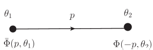
Figure 1: Scalar superfield propagator

We have chosen the convention for the momentum flow direction to be from $\bar{\Phi}$ to $\Phi$ (see fig 1). Our sign conventions are such that the momenta leaving a vertex have a positive sign. The notation $D^{2}_{\theta_{1},p}$ means that the operator depends on $\theta_{1}$ and the momentum $p$, the explicit form for $D^{2}$ and some useful formulae are listed in §A.2. The gauge superfield propagator in momentum space is

$$\langle\Gamma^{-}(\theta_{1},p)\Gamma^{-}(\theta_{2},-p^{\prime})\rangle=-\frac{8\pi}{\kappa}\frac{\delta^{2}(\theta_{1}-\theta_{2})}{p_{--}}(2\pi)^{3}\delta^{3}(p-p^{\prime})\$$ (109)

where $p_{--}=-(p_{1}+ip_{2})=-p_{-}$.

Figure 2: Gauge superfield propagator, the arrow indicates direction of momentum flow

Inserting the expansion (2.1) into the LHS of (109) and matching powers of $\theta$, we find in particular that

$$\langle A_{+}(p)A_{3}(-p^{\prime})\rangle=\frac{4\pi i}{\kappa}\frac{1}{p_{-}}(2\pi)^{3}\delta^{3}(p-p^{\prime})\ ,\ \langle A_{3}(p)A_{+}(-p^{\prime})\rangle=-\frac{4\pi i}{\kappa}\frac{1}{p_{-}}(2\pi)^{3}\delta^{3}(p-p^{\prime})\ ,\$$ (110)

is in perfect agreement with the propagator of the gauge field in regular (non-supersymmetric) lightcone gauge (see Appendix A ,Eq A.7 of Giombi:2011kc )

3.3 The all orders matter propagator

3.3.1 Constraints from supersymmetry

The exact propagator of the matter superfield $\Phi$ enjoys invariance under supersymmetry transformations which implies that

$$(Q_{\theta_{1},p}+Q_{\theta_{2},-p})\langle\bar{\Phi}(\theta_{1},p)\Phi(\theta_{2},-p)\rangle=0$$ (111)

where the supergenerators $Q_{\theta_{1},p}$ were defined in (9). This constraint is easily solved. Let the exact scalar propagator take the form

$$\langle\bar{\Phi}(p,\theta_{1})\Phi(-p^{\prime},\theta_{2})\rangle=(2\pi)^{3}\delta^{3}(p-p^{\prime})P(\theta_{1},\theta_{2},p)\ .$$ (112)

The condition (111) implies that the function $P$ obeys the equation

$$\bigg{[}\frac{\partial}{\partial\theta_{1}^{\alpha}}+\frac{\partial}{\partial\theta_{2}^{\alpha}}-p_{\alpha\beta}(\theta_{1}^{\beta}-\theta_{2}^{\beta})\bigg{]}P(\theta_{1},\theta_{2},p)=0\ .$$ (113)

The most general solution to (113) is

$$C_{1}(p^{\mu})\exp(-\theta_{1}^{\alpha}p_{\alpha\beta}\theta_{2}^{\beta})+C_{2}(p^{\mu})\delta^{2}(\theta_{1}-\theta_{2})\$$ (114)

or equivalently

$$P(\theta_{1},\theta_{2},p) =\exp(-\theta_{1}^{\alpha}p_{\alpha\beta}\theta_{2}^{\beta})\left(C_{1}(p^{\mu})+C_{2}(p^{\mu})\delta^{2}(\theta_{1}-\theta_{2})\right)\$$ (115)

where $C_{1}(p^{\mu})$ is an arbitrary function of $p^{\mu}$ of dimension $m^{-2}$, while $C_{2}(p^{\mu})$ is another function of $p^{\mu}$ of dimension $m^{-1}$.

It is easily verified using the formulae (280) that the bare propagator (108) can be recast in the form (115) with

$$C_{1}=\frac{1}{p^{2}+m_{0}^{2}}\ ,\ C_{2}=\frac{m_{0}}{p^{2}+m_{0}^{2}}\ .$$ (116)

In a similar manner supersymmetry constrains the terms quadratic in $\Phi$ and ${\bar{\Phi}}$ in the quantum effective action. In momentum space the most general supersymmetric quadratic effective action takes the form

$$S =-\int\frac{d^{3}p}{(2\pi)^{3}}d^{2}\theta\bar{\Phi}(p,\theta)\left(A(p)D^{2}+B(p)\right)\Phi(-p,\theta)$$ (117)

$$=-\int\frac{d^{3}p}{(2\pi)^{3}}d^{2}\theta_{1}d^{2}\theta_{2}\bar{\Phi}(p,\theta_{1})\exp(-\theta_{1}^{\alpha}p_{\alpha\beta}\theta_{2}^{\beta})(A(p)+B(p)\delta^{2}(\theta_{1}-\theta_{2}))\Phi(-p,\theta_{2})$$ (118)

The tree level quadratic action of our theory is clearly of the form (117) with $A(p)=1$ and $B(p)=m_{0}$.

3.3.2 All orders two point function

Let the exact 1PI quadratic effective action take the form

$$S_{2}=\int\frac{d^{3}p}{(2\pi)^{3}}d^{2}\theta_{1}d^{2}\theta_{2}\bar{\Phi}(-p,\theta_{1})\left(\exp(-\theta_{1}^{\alpha}p_{\alpha\beta}\theta_{2}^{\beta})+m_{0}\delta^{2}(\theta_{1}-\theta_{2})+\Sigma(p,\theta_{1},\theta_{2})\right)\Phi(p,\theta_{2})\ .$$ (119)

It follows from (117) that the supersymmetric self energy $\Sigma$ is of the form

$$\Sigma(p,\theta_{1},\theta_{2})=C(p)\exp(-\theta_{1}^{\alpha}p_{\alpha\beta}\theta_{2}^{\beta})+D(p)\delta^{2}(\theta_{1}-\theta_{2})$$ (120)

where $C(p)$ and $D(p)$ are as yet unknown functions of momenta.

Imitating the steps described in section 3 of Giombi:2011kc , the self energy $\Sigma$

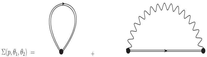
Figure 3: Integral equation for self energy

defined in (119) may be shown to obey the integral equation

$$\Sigma(p,\theta_{1},\theta_{2})= \ 2\pi\lambda w\int\frac{d^{3}r}{(2\pi)^{3}}\delta^{2}(\theta_{1}-\theta_{2})P(r,\theta_{1},\theta_{2})$$

$$-2\pi\lambda\int\frac{d^{3}r}{(2\pi)^{3}}D^{\theta_{2},-p}_{-}D^{\theta_{1},p}_{-}\left(\frac{\delta^{2}(\theta_{1}-\theta_{2})}{(p-r)_{--}}P(r,\theta_{1},\theta_{2})\right)$$

$$+2\pi\lambda\int\frac{d^{3}r}{(2\pi)^{3}}\frac{\delta^{2}(\theta_{1}-\theta_{2})}{(p-r)_{--}}D_{-}^{\theta_{1},r}D_{-}^{\theta_{2},-r}P(r,\theta_{1},\theta_{2})$$ (121)

where $P(p,\theta_{1},\theta_{2})$ is the exact superfield propagator. Note that the propagator $P$ depends on $\Sigma$ (in fact $P$ is obtained by inverting quadratic term in effective action (119)). In other words $\Sigma$ appears both on the LHS and RHS of (3.3.2); we need to solve this equation to determine $\Sigma$.

Using the equations (A.2), the second and third lines on the RHS if (3.3.2) may be considerably simplified (see Appendix §G) and we find

$$\Sigma(p,\theta_{1},\theta_{2})= \ 2\pi\lambda w\int\frac{d^{3}r}{(2\pi)^{3}}\delta^{2}(\theta_{1}-\theta_{2})P(r,\theta_{1},\theta_{2})$$

$$-2\pi\lambda\int\frac{d^{3}r}{(2\pi)^{3}}\frac{p_{--}}{(p-r)_{--}}\delta^{2}(\theta_{1}-\theta_{2})P(r,\theta_{1},\theta_{2})$$

$$+2\pi\lambda\int\frac{d^{3}r}{(2\pi)^{3}}\frac{r_{--}}{(p-r)_{--}}\delta^{2}(\theta_{1}-\theta_{2})P(r,\theta_{1},\theta_{2})$$ (122)

Combining the second and third lines on the RHS of (3.3.2) we see that the factors of $p_{--}$ and $r_{--}$ cancel perfectly between the numerator and denominator, and (3.3.2) simplifies to

$$\Sigma(p,\theta_{1},\theta_{2})= \ 2\pi\lambda(w-1)\int\frac{d^{3}r}{(2\pi)^{3}}\delta^{2}(\theta_{1}-\theta_{2})P(r,\theta_{1},\theta_{2})\ .$$ (123)

Notice that the RHS of (123) is independent of $p$, so it follows that

$$\Sigma(p,\theta_{1},\theta_{2})=(m-m_{0})\delta^{2}(\theta_{1}-\theta_{2})$$

for some as yet undetermined constant $m$. It follows that the exact propagator $P$ takes the form of the tree level propagator with $m_{0}$ replaced by $m$ i.e.

$$P(p,\theta_{1},\theta_{2})=\frac{D^{2}-m}{p^{2}+m^{2}}\delta^{2}(\theta_{1}-\theta_{2})\ .$$ (124)

Plugging (124) into (123) and simplifying we find the equation

$$m-m_{0} =2\pi\lambda(w-1)\int\frac{d^{3}r}{(2\pi)^{3}}\frac{1}{r^{2}+m^{2}}\ .$$ (125)

The integral on the RHS diverges. Regulating this divergence using dimensional regularization, we find that (125) reduces to

$$m-m_{0}=\frac{\lambda|m|}{2}(1-w)$$ (126)

and so

$$m=\frac{2m_{0}}{2+(-1+w)\lambda\ \text{Sgn(m)}}\ .$$ (127)

Let us summarize. The exact 1PI quadratic effective action for the $\Phi$ superfield has the same form as the tree level effective action but with the bare mass $m_{0}$ replaced by the exact mass $m$ given in (127). As explained in §2.2 the exact mass (127) is duality invariant.

Note also that the $\mathcal{N}=2$ point, $w=1$ there is no renormalization of the mass, and the bare propagator is exact and the bare mass (which equals the pole mass) is itself duality invariant.

3.4 Constraints from supersymmetry on the offshell four point function

Much as with the two point function, the offshell four point function of matter superfields is constrained by the supersymmetric Ward identities. Let us define

$$\langle\bar{\Phi}((p+q+\frac{l}{4}),\theta_{1})\Phi(-p+\frac{l}{4},\theta_{2})\Phi(-(k+q)+\frac{l}{4},\theta_{3})\bar{\Phi}(k+\frac{l}{4},\theta_{4})\rangle$$

$$=(2\pi)^{3}\delta(l)V(\theta_{1},\theta_{2},\theta_{3},\theta_{4},p,q,k).$$ (128)

It follows from the invariance under supersymmetry that

$$(Q_{\theta_{1},p+q}+Q_{\theta_{2},-p}+Q_{\theta_{3},-k-q}+Q_{\theta_{4},k})V(\theta_{1},\theta_{2},\theta_{3},\theta_{4},p,q,k)=0\ .$$ (129)

The general solution to (129) is easily obtained (see Appendix §H.1). Defining

$$X=\sum_{i=1}^{4}\theta_{i}\ ,$$

$$X_{12}=\theta_{1}-\theta_{2}\ ,$$

$$X_{13}=\theta_{1}-\theta_{3}\ ,$$

$$X_{43}=\theta_{4}-\theta_{3}\ .$$ (130)

we find

$$V=\exp\bigg{(}\frac{1}{4}X.(p.X_{12}+q.X_{13}+k.X_{43})\bigg{)}F(X_{12},X_{13},X_{43},p,q,k)\ .$$ (131)

where $F$ is an unconstrained function of its arguments. In other words supersymmetry fixes the transformation of $V$ under a uniform shift of all $\theta$ parameters $\theta_{i}\rightarrow\theta_{i}+\gamma$. (for $i=1\ldots 4$ where $\gamma$ is a constant Grassman parameter). The undetermined function $F$ is a function of shift invariant combinations of the four $\theta_{i}$.

Let us now turn to the structure of the exact 1PI effective action for scalar superfields in our theory. The most general effective action consistent with global $U(N)$ invariance and supersymmetry takes the form

$$\begin{split}S_{4}&=\frac{1}{2}\int\frac{d^{3}p}{(2\pi)^{3}}\frac{d^{3}k}{(2\pi)^{3}}\frac{d^{3}q}{(2\pi)^{3}}d^{2}\theta_{1}d^{2}\theta_{2}d^{2}\theta_{3}d^{2}\theta_{4}\\ &\left(V(\theta_{1},\theta_{2},\theta_{3},\theta_{4},p,q,k)\Phi_{m}(-(p+q),\theta_{1}){\bar{\Phi}}^{m}(p,\theta_{2}){\bar{\Phi}}^{n}(k+q,\theta_{3})\Phi_{n}(-k,\theta_{4})\right)\ .\\ \end{split}$$ (132)

It follows from the definition (132) that the function $V$ may be taken to be invariant under the $Z_{2}$ symmetry

$$p\rightarrow k+q,k\rightarrow p+q,q\rightarrow-q\ ,$$

$$\theta_{1}\rightarrow\theta_{4},\theta_{2}\rightarrow\theta_{3},\theta_{3}\rightarrow\theta_{2},\theta_{4}\rightarrow\theta_{1}\ .$$ (133)

As in the case of two point functions, it is easily demonstrated that the invariance of this action under supersymmetry constraints the coefficient function $V$ that appears in (132) to obey the equation (129). As we have already explained above, the most general solution to this equation is given in equation (131) for a general shift invariant function $F$.

3.5 An integral equation for the offshell four point function

The coefficient function $V$ of the quartic term of the exact IPI effective action may be shown to obey the integral equation (see Fig 4 for a diagrammatic representation of this equation)

$$V(\theta_{1},\theta_{2},\theta_{3},\theta_{4},p,q,k)=\ V_{0}(\theta_{1},\theta_{2},\theta_{3},\theta_{4},p,q,k)$$

$$+\int\frac{d^{3}r}{(2\pi)^{3}}d^{2}\theta_{a}d^{2}\theta_{b}d^{2}\theta_{A}d^{2}\theta_{B}\bigg{(}NV_{0}(\theta_{1},\theta_{2},\theta_{a},\theta_{b},p,q,r)$$

$$\qquad P(r+q,\theta_{a},\theta_{A})P(r,\theta_{B},\theta_{b})V(\theta_{A},\theta_{B},\theta_{3},\theta_{4},r,q,k)\bigg{)}\$$ (134)

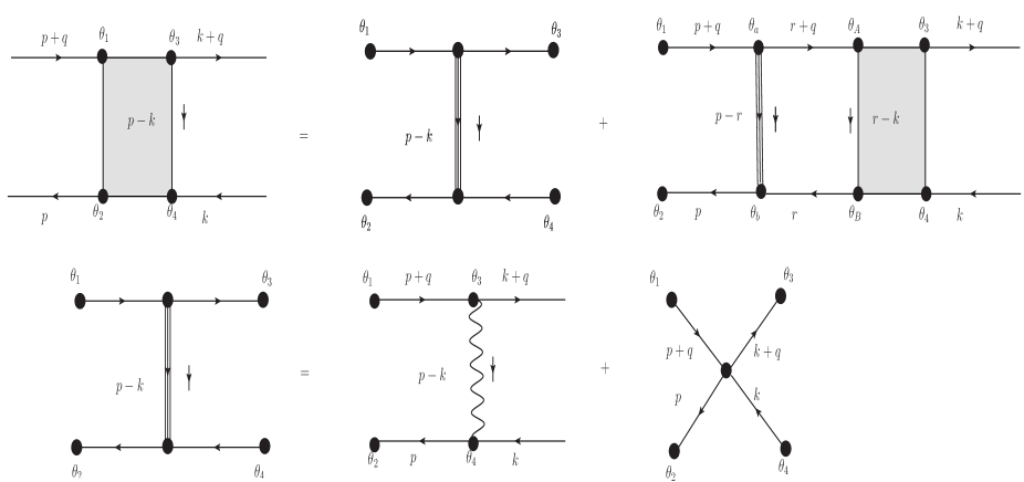
Figure 4: The diagrams in the first line pictorially represents the Schwinger-Dyson equation for offshell four point function (see (3.5)). The second line represents the tree level contributions from the gauge superfield interaction and the quartic interactions.

In (3.5) $V_{0}$ is the tree level contribution to $V$. $V_{0}$ receives contributions from the two diagrams depicted in Fig 4. The explicit evaluation of $V_{0}$ is a straightforward exercise and we find (see Appendix §H.2 for details)

$$V_{0}(\theta_{1},\theta_{2},\theta_{3},\theta_{4},p,q,k)= \exp\bigg{(}\frac{1}{4}X.(p.X_{12}+q.X_{13}+k.X_{43})\bigg{)}$$

$$\ \ \biggl{(}-\frac{i\pi w}{\kappa}X_{12}^{-}X_{12}^{+}X_{13}^{-}X_{13}^{+}X_{43}^{-}X_{43}^{+}$$

$$\ \ \ \ -\frac{4\pi i}{\kappa(p-k)_{--}}X_{12}^{+}X_{13}^{+}X_{43}^{+}(X_{12}^{-}+X_{34}^{-})\biggr{)}\ .$$ (135)

In the above, the first term in the bracket is the delta function from the quartic interaction, the second term is from the tree diagram due to the gauge superfield exchange computed in §H.2.

We now turn to the evaluation of the coefficient $V$ in the exact 1PI effective action. There are $2^{6}$ linearly independent functions of the six independent shift invariant Grassman variables $X_{12}^{\pm}$, $X_{13}^{\pm}$ and $X_{43}^{\pm}$. Consequently the most general $V$ consistent with supersymmetry is parameterized by 64 unknown functions of the three independent momenta. $V$ (and so $F$) is necessarily an even function of these variables. It follows that the most general function $F$ can be parameterized in terms of 32 bosonic functions of $p,k$ and $q$. In principle one could insert the most general supersymmetric $F$ into the integral equation (3.5) and equate equal powers of $\theta_{i}$ on the two sides of (3.5) to obtain 32 coupled integral equations for the 32 unknown complex valued functions. One could, then, attempt to solve this system of equations. This procedure would obviously be very complicated and difficult to implement in practice. Focusing on the special kinematics $q^{\pm}=0$ we were able to shortcircuit this laborious process, in a manner we now describe.

After a little playing around we were able to demonstrate that $V$ of the form

$$V(\theta_{1},\theta_{2},\theta_{3},\theta_{4},p,q,k)=\exp\bigg{(}\frac{1}{4}X .(p.X_{12}+q.X_{13}+k.X_{43})\bigg{)}F(X_{12},X_{13},X_{43},p,q,k)$$

$$F(X_{12},X_{13},X_{43},p,q,k)=\begin{split}X_{12}^{+}X_{43}^{+}\bigg{(}&A(p,k,q)X_{12}^{-}X_{43}^{-}X_{13}^{+}X_{13}^{-}+B(p,k,q)X_{12}^{-}X_{43}^{-}\\ &+C(p,k,q)X_{12}^{-}X_{13}^{+}+D(p,k,q)X_{13}^{+}X_{43}^{-}\bigg{)}\end{split}\ ,$$

is closed under the multiplication rule induced by the RHS of (3.5) (see Appendix §H.3). Plugging in the general form of $V$ (3.5) in the integral equation (3.5) and performing the grassmann integration, (3.5) turns into to the following integral equations for the coefficient functions $A$, $B$, $C$ and $D$:

$$A(p,k,q)+\frac{2\pi iw}{\kappa}$$

$$+i\pi\lambda\int\frac{d^{3}r_{E}}{(2\pi)^{3}}\frac{2A(q_{3}p_{-}+2(q_{3}-im)r_{-})+(q_{3}r_{-}+2imp_{-})(2Bq_{3}+Ck_{-})-Dr_{-}(q_{3}p_{-}+2imr_{-})}{(r^{2}+m^{2})((r+q)^{2}+m^{2})(p-r)_{-}}$$

$$-i\pi\lambda w\int\frac{d^{3}r_{E}}{(2\pi)^{3}}\frac{4iAm+2Bq_{3}^{2}+Cq_{3}k_{-}+2D(q_{3}+im)r_{-}}{(r^{2}+m^{2})((r+q)^{2}+m^{2})}=0$$ (137)

$$B(p,k,q) +i\pi\lambda\int\frac{d^{3}r_{E}}{(2\pi)^{3}}\frac{2A(p+r)_{-}+4B(q_{3}r_{-}+im(p-r)_{-})-Ck_{-}(p+r)_{-}-Dr_{-}(p-3r)_{-}}{(r^{2}+m^{2})((r+q)^{2}+m^{2})(p-r)_{-}}$$

$$-i\pi\lambda w\int\frac{d^{3}r_{E}}{(2\pi)^{3}}\frac{2A+4imB-Ck_{-}-Dr_{-}}{(r^{2}+m^{2})((r+q)^{2}+m^{2})}=0$$ (138)

$$C(p,k,q)-\frac{4\pi i}{\kappa(p-k)_{-}} +i\pi\lambda\int\frac{d^{3}r_{E}}{(2\pi)^{3}}\frac{2C\big{(}q_{3}(p+3r)_{-}+2im(p-r)_{-}\big{)}}{(r^{2}+m^{2})((r+q)^{2}+m^{2})(p-r)_{-}}$$

$$-i\pi\lambda w\int\frac{d^{3}r_{E}}{(2\pi)^{3}}\frac{2C(q_{3}+2im)}{(r^{2}+m^{2})((r+q)^{2}+m^{2})}=0$$ (139)

$$D(p,k,q)-\frac{4\pi i}{\kappa(p-k)_{-}}$$

$$+i\pi\lambda\int\frac{d^{3}r_{E}}{(2\pi)^{3}}\frac{-A(4q_{3}-8im)+(q_{3}-2im)(4Bq_{3}+2Ck_{-})+2D(3q_{3}+2im)r_{-}}{(r^{2}+m^{2})((r+q)^{2}+m^{2})(p-r)_{-}}=0\ .$$ (140)

We will sometimes find it useful to view the four integral equations above as a single integral equation for a four dimensional column vector $E$ whose components are the functions $A$, $B$, $C$, $D$, i.e.

$$E(p,k,q)=\left(\begin{array}[]{c}A(p,k,q)\\ B(p,k,q)\\ C(p,k,q)\\ D(p,k,q)\end{array}\right)\ .$$ (141)

The integral equations take the schematic form

$$E=R+IE$$ (142)

where $R$ is a 4 column of functions and $I$ is a matrix of integral operators acting on $E$. The integral equation (142) may be converted into a differential equation by differentiating both sides of (142) w.r.t $p_{+}$. Using (460) and performing all $d^{3}r$ integrals (using (458) for the integral over $r_{3}$) we obtain the differential equations

$$\partial_{p_{+}}E(p,k,q)=S(p,k,q)+H(p,k_{-},q)E(p,k,q)\ ,$$ (143)

where

$$S(p,k,q)=-\frac{8i\pi^{2}}{\kappa}\delta^{2}((p-k)_{-},(p-k)_{+})\left(\begin{array}[]{c}0\\ 0\\ 1\\ 1\end{array}\right)$$ (144)

$$H(p,k_{-},q_{3})=\frac{1}{a(p_{s},q_{3})}\left(\begin{array}[]{cccc}(6q_{3}-4im)p_{-}&2q_{3}(2im+q_{3})p_{-}&(2im+q_{3})k_{-}p_{-}&-(2im+q_{3})p_{-}^{2}\\ 4p_{-}&4q_{3}p_{-}&-2k_{-}p_{-}&2p_{-}^{2}\\ 0&0&8q_{3}p_{-}&0\\ 8im-4q_{3}&4q_{3}(q_{3}-2im)&2(q_{3}-2im)k_{-}&(4im+6q_{3})p_{-}\\ \end{array}\right)$$ (145)

and

$$a(p_{s},q_{3})=\frac{\sqrt{m^{2}+p_{s}^{2}}\left(4m^{2}+q_{3}^{2}+4p_{s}^{2}\right)}{2\pi}\ .$$ (146)

As we have explained above, the exact vertex $V$ enjoys invariance under the $\mathbb{Z}_{2}$ transformation (3.4). In terms of the functions $A,B,C,D$, the $\mathbb{Z}_{2}$ action is given by

$$E(p,k,q)=TE(k,p,-q)\ ,$$ (147)

where

$$T=\left(\begin{array}[]{cccc}1&0&0&0\\ 0&1&0&0\\ 0&0&0&-1\\ 0&0&-1&0\end{array}\right)\ .$$ (152)

The differential equations (143) do not manifestly respect the invariance (147). In fact in Appendix §H.4 we have demonstrated that the differential equations (143) admit solutions that enjoy the invariance (147) if and only if the following consistency condition is obeyed:

$$[H(p,k_{-},q),TH(k,p_{-},-q)T]=0\ .$$ (153)

In the same Appendix we have also explicitly verified that this integrability condition is in fact obeyed; this is a consistency check on (143) and indirectly on the underlying integral equations.

3.6 Explicit solution for the offshell four point function

In this subsection, we solve the system of integral equations for the unknown functions $A,B,C,D$ presented in the previous subsection. We propose the ansatz

$$A(p,k,q)=A_{1}(p_{s},k_{s},q_{3})+\frac{A_{2}(p_{s},k_{s},q_{3})k_{-}}{(p-k)_{-}}\ ,$$

$$B(p,k,q)=B_{1}(p_{s},k_{s},q_{3})+\frac{B_{2}(p_{s},k_{s},q_{3})k_{-}}{(p-k)_{-}}\ ,$$

$$C(p,k,q)=-\frac{C_{2}(p_{s},k_{s},q_{3})-C_{1}(p_{s},k_{s},q_{3})k_{+}p_{-}}{(p-k)_{-}}\ ,$$

$$D(p,k,q)=-\frac{D_{2}(p_{s},k_{s},q_{3})-D_{1}(p_{s},k_{s},q_{3})k_{-}p_{+}}{(p-k)_{-}}\ .$$ (154)

Our ansatz (3.6) fixes the solution in terms of 8 unknown functions of $p_{s},k_{s}$ and $q_{3}$.

Plugging the ansatz (3.6) into the integral equations (3.5)-(3.5), one can do the angle and $r_{3}$ integrals (using the formulae (H.5) and (458) respectively) leaving only the $r_{s}$ integral to be performed. Differentiating this expression w.r.t. to $p_{s}$ turns out to kill the $r_{s}$ integral yielding differential equations in $p_{s}$ for the eight equations above. The resulting differential equations turn out to be exactly solvable. Assuming that the solution respects the symmetry (147), it turns out to be given in terms of two unknown functions of $k_{s}$ and $q_{3}$. These can be thought of as the integration constants that are not fixed by the symmetry requirement (147). Plugging the solutions back into the integral equations we were able to determine these two integration functions of $k_{s}$ and $q_{3}$ completely. We now report our results.

The solutions for $A$ and $B$ are

$$A_{1}(p_{s},k_{s},q_{3})= e^{-2i\lambda\tan^{-1}\frac{2\sqrt{m^{2}+p_{s}^{2}}}{q_{3}}}\biggl{(}G_{1}(k_{s},q_{3})$$

$$+\frac{2\pi(w-1)(2m-iq_{3})e^{2i\lambda\big{(}\tan^{-1}\frac{2\sqrt{k_{s}^{2}+m^{2}}}{q_{3}}+\tan^{-1}\frac{2\sqrt{m^{2}+p_{s}^{2}}}{q_{3}}\big{)}}}{\kappa(e^{\frac{i\pi\lambda q_{3}}{|q_{3}|}}(q_{3}(w+3)-2im(w-1))+i(w-1)(2m+iq_{3})e^{2i\lambda\tan^{-1}\frac{2|m|}{q_{3}}})}\biggr{)}\ ,$$

$$A_{2}(p_{s},k_{s},q_{3})= e^{-2i\lambda\tan^{-1}\left(\frac{2\sqrt{m^{2}+p_{s}^{2}}}{q_{3}}\right)}G_{2}(k_{s},q_{3})\ ,$$

$$B_{1}(p_{s},k_{s},q_{3})= \frac{2\pi A_{1}(p_{s},k_{s},q_{3})}{q_{3}}$$

$$+\frac{2\pi}{b_{1}b_{2}}\biggl{(}-i(w-1)^{2}(4m^{2}+q_{3}^{2})e^{i\lambda\big{(}\frac{\pi q_{3}}{|q_{3}|}-2\tan^{-1}\frac{2\sqrt{m^{2}+p_{s}^{2}}}{q_{3}}+4\tan^{-1}\frac{2|m|}{q_{3}}\big{)}}$$

$$+i(w-1)^{2}(-4m^{2}+8imq_{3}+3q_{3}^{2})e^{i\lambda\big{(}\frac{\pi q_{3}}{|q_{3}|}+2\tan^{-1}\frac{2\sqrt{k_{s}^{2}+m^{2}}}{q_{3}}\big{)}}$$

$$-8iq_{3}^{2}(w+1)e^{i\lambda\big{(}\frac{\pi q_{3}}{|q_{3}|}+2(\tan^{-1}\frac{2\sqrt{k_{s}^{2}+m^{2}}}{q_{3}}-\tan^{-1}\frac{2\sqrt{m^{2}+p_{s}^{2}}}{q_{3}}+\tan^{-1}\frac{2|m|}{q_{3}})\big{)}}$$

$$+(w-1)(q_{3}+2im)(2m(w-1)+iq_{3}(w+3))+e^{2i\lambda(\frac{\pi q_{3}}{|q_{3}|}-\tan^{-1}\frac{2\sqrt{m^{2}+p_{s}^{2}}}{q_{3}}+\tan^{-1}\frac{2|m|}{q_{3}})}$$

$$+(w-1)(2m-3iq_{3})(q_{3}(w+3)+2im(w-1))+e^{2i\lambda\big{(}\tan^{-1}\frac{2\sqrt{k_{s}^{2}+m^{2}}}{q_{3}}+\tan^{-1}\frac{2|m|}{q_{3}}\big{)}}\biggr{)}\ ,$$

$$B_{2}(p_{s},k_{s},q_{3})= \frac{A_{2}(p_{s},k_{s},q_{3})}{q_{3}}\ ,$$

$$G_{1}(k_{s},q_{3})= -\frac{2\pi}{\kappa}\frac{1}{g_{1}}\biggl{(}-8iq_{3}^{2}(w+1)e^{i\lambda\big{(}\frac{\pi q_{3}}{|q_{3}|}+2(\tan^{-1}\frac{2\sqrt{k_{s}^{2}+m^{2}}}{q_{3}}+\tan^{-1}\frac{2|m|}{q_{3}})\big{)}}$$

$$+i(w-1)^{2}(q_{3}-2im)^{2}e^{i\lambda\big{(}\frac{\pi q_{3}}{|q_{3}|}+4\tan^{-1}\frac{2|m|}{q_{3}}\big{)}}$$

$$-(w-1)(q_{3}-2im)(2m(w-1)+iq_{3}(w+3))e^{2i\lambda\big{(}\frac{\pi q_{3}}{|q_{3}|}+\tan^{-1}\frac{2|m|}{q_{3}}\big{)}}\biggr{)}\ ,$$

$$G_{2}(k_{s},q_{3})= 0\ ,$$ (155)

where we have defined some parameters as given below for ease of presentation.

$$g_{1}= (w-1)(q_{3}+2im)e^{\frac{2i\pi\lambda q_{3}}{|q_{3}|}}(q_{3}(w+3)-2im(w-1))\ ,$$

$$+(w-1)(4m^{2}(w-1)-8imq_{3}+q_{3}^{2}(w+3))e^{4i\lambda\tan^{-1}\frac{2|m|}{q_{3}}}\ ,$$

$$-2(4m^{2}(w-1)^{2}+q_{3}^{2}(w^{2}+2w+5))e^{i\lambda(\frac{\pi q_{3}}{|q_{3}|}+2\tan^{-1}\frac{2|m|}{q_{3}})}\ ,$$

$$b_{1}= \kappa q_{3}((w-1)(q_{3}+2im)e^{\frac{i\pi\lambda q_{3}}{|q_{3}|}}+(-q_{3}(w+3)-2im(w-1))e^{2i\lambda\tan^{-1}\frac{2|m|}{q_{3}}})\ ,$$

$$b_{2}= e^{\frac{i\pi\lambda q_{3}}{|q_{3}|}}(q_{3}(w+3)-2im(w-1))+i(w-1)(2m+iq_{3})e^{2i\lambda\tan^{-1}\frac{2|m|}{q_{3}}}\ ,$$

The solutions for C and D are

$$C_{1}(p_{s},k_{s},q_{3})= \frac{4\pi(q_{3}+2im)(e^{2i\lambda\tan^{-1}\frac{2|m|}{q_{3}}}-e^{2i\lambda\tan^{-1}\frac{2\sqrt{k_{s}^{2}+m^{2}}}{q_{3}}})e^{i\lambda(\frac{\pi q_{3}}{|q_{3}|}-2\tan^{-1}\frac{2\sqrt{m^{2}+p_{s}^{2}}}{q_{3}})}}{\kappa k_{s}^{2}(i(q_{3}+2im)e^{\frac{i\pi\lambda q_{3}}{|q_{3}|}}+(2m-iq_{3}\left(\frac{w+3}{w-1}\right))e^{2i\lambda\tan^{-1}\frac{2|m|}{q_{3}}})}\ ,$$

$$C_{2}(p_{s},k_{s},q_{3})= \frac{4\pi e^{2i\lambda(\tan^{-1}\frac{2|m|}{q_{3}}-\tan^{-1}\frac{2\sqrt{m^{2}+p_{s}^{2}}}{q_{3}})}((q_{3}+2im)e^{\frac{i\pi\lambda q_{3}}{|q_{3}|}}-(q_{3}\left(\frac{w+3}{w-1}\right)+2im)e^{2i\lambda\tan^{-1}\frac{2\sqrt{k_{s}^{2}+m^{2}}}{q_{3}}})}{\kappa(i(q_{3}+2im)e^{\frac{i\pi\lambda q_{3}}{|q_{3}|}}+(2m-iq_{3}\left(\frac{w+3}{w-1}\right))e^{2i\lambda\tan^{-1}\frac{2|m|}{q_{3}}})}\ ,$$

$$D_{1}(p_{s},k_{s},q_{3})= C_{1}(k_{s},p_{s},-q_{3})\ ,$$

$$D_{2}(p_{s},k_{s},q_{3})= C_{2}(k_{s},p_{s},-q_{3})\ .$$ (157)

It is straightforward to show that the above solutions satisfy the various symmetry requirements that follow from (147).

Although the solutions (3.6) and (3.6) are quite complicated, a drastic simplification occurs at the $\mathcal{N}=2$ point $w=1$

$$A= -\frac{2i\pi e^{2i\lambda\big{(}\tan^{-1}\frac{2\sqrt{k_{s}^{2}+m^{2}}}{q_{3}}-\tan^{-1}\frac{2\sqrt{m^{2}+p_{s}^{2}}}{q_{3}}\big{)}}}{\kappa}\ ,$$

$$B= \ 0\ ,$$

$$C= -\frac{4i\pi e^{2i\lambda\big{(}\tan^{-1}\frac{2\sqrt{k_{s}^{2}+m^{2}}}{q_{3}}-\tan^{-1}\frac{2\sqrt{m^{2}+p_{s}^{2}}}{q_{3}}\big{)}}}{\kappa(k-p)_{-}}\ ,$$

$$D= -\frac{4i\pi e^{2i\lambda\big{(}\tan^{-1}\frac{2\sqrt{k_{s}^{2}+m^{2}}}{q_{3}}-\tan^{-1}\frac{2\sqrt{m^{2}+p_{s}^{2}}}{q_{3}}\big{)}}}{\kappa(k-p)_{-}}\ .$$ (158)

It is satisfying that the complicated results of the general $\mathcal{N}=1$ theory collapse to an extremely simple form at the $\mathcal{N}=2$ point.

3.7 Onshell limit and the $S$ matrix

The explicit solution for the functions $A$, $B$, $C$ and $D$, presented in the previous subsection, completely determine $V$ in (132), and so the quadratic part of the exact (large $N$) IPI effective action. The most general $2\times 2$ $S$ matrix may now be obtained from (132) as follows. We simply substitute the onshell expressions

$$\Phi(p,\theta)=(2\pi)\delta(p^{2}+m^{2})\bigg{[} \theta(p^{0})\bigg{(}a(\mathbf{p})(1+m\theta^{2})+\theta^{\alpha}u_{\alpha}(\mathbf{p})\alpha(\mathbf{p})\bigg{)}$$

$$+\theta(-p^{0})\bigg{(}a^{c{\dagger}}(-\mathbf{p})(1+m\theta^{2})+\theta^{\alpha}v_{\alpha}(-\mathbf{p})\alpha^{c{\dagger}}(-\mathbf{p})\bigg{)}\bigg{]}$$ (159)

into (132) (here $a$ and $\alpha$ are the effectively free oscillators that create and destroy particles at very early or very late times; these oscillators obey the commutation relations (33)). Performing the integrals over $\theta^{\alpha}$ reduces (132) to a quartic form (let us call it $L$) in bosonic and fermionic oscillators. The $S$ matrix is obtained by sandwiching the resultant expression between the appropriate in and out states, and evaluating the resulting matrix elements using the commutation relations (33).

It may be verified that the quartic form in oscillators takes the form

$$L=\sum_{\phi_{i}=0,\pi}\int\prod_{i=1}^{4} d\theta_{i}\frac{d^{3}p_{i}}{((2\pi)^{3})^{4}}\delta(p_{i}^{2}+m^{2})S_{M}(p_{1},\phi_{1},\theta_{1},p_{2},\phi_{2},\theta_{2},p_{3},\phi_{3},\theta_{3},p_{4},\phi_{4},\theta_{4})$$

$$\left(\delta_{\phi_{i},0}\theta(p^{0}_{i})A(p_{i},\phi_{i},\theta_{i})+\delta_{\phi_{i},\pi}\theta(-p^{0}_{i})\tilde{A}(-p_{i},\phi_{i},\theta_{i})\right)(2\pi)^{3}\delta^{3}(p_{1}+p_{2}+p_{3}+p_{4})$$

where

$$A(p_{i},\phi_{i},\theta_{i})=a(\mathbf{p}_{i})+\alpha(\mathbf{p}_{i})e^{-\frac{i\phi_{i}}{2}}\theta_{i}\ ,$$

$$\tilde{A}(p_{i},\phi_{i},\theta_{i})=a^{\dagger}(\mathbf{p}_{i})+e^{-\frac{i\phi_{i}}{2}}\theta_{i}\alpha^{\dagger}(\mathbf{p}_{i})\ ,$$ (160)

where the one component fermionic variables $\theta_{i}$ are the fermionic variables that parameterize onshell superspace (see §2.4 ) and the master formula is defined in (53). Note that the phase variables $\phi_{i}$ are summed over two values $0$ and $\pi$; the symbol $\delta_{\phi,0}$ is unity when $\phi=0$ but zero when $\phi=\pi$ and $\delta_{\phi,\pi}$ has an analogous definition. (3.7) compactly identifies the coefficient of every quartic form in oscillators. For instance it asserts that the coefficient of $a_{1}a_{2}a_{3}^{\dagger}a_{4}^{\dagger}$ is the $S$ matrix for scattering bosons with momentum $p_{1},p_{2}$ to bosons with momenta $p_{3},p_{4}$, while the the coefficient of $\alpha_{2}\alpha_{4}a_{1}^{\dagger}a_{3}^{\dagger}$ is minus the $S$ matrix for scattering fermions with momentum $p_{2},p_{4}$ to bosons with momentum $p_{1},p_{3}$, etc.

We can use the $\delta$ function in (3.7) to perform the integral over one of the four momenta; the integral over the remaining momenta may be recast as an integral over the momenta $p$ $k$ and $q$ employed in the previous section; specifically (see Fig 4 )

$$p_{1}=p+q\ ,\ p_{2}=-k-q\ ,\ p_{3}=-p\ ,\ p_{4}=k\ .$$ (161)

From the explicit results we get by substituting (3.7) into (132) we can read off all $S$ matrices at $q_{\pm}=0$.

To start with, let us restrict our attention to the bosonic sector. From direct computation we find that in this sector (3.7) reduces to

$$L_{B}=\sum_{\phi_{i}=0,\pi}\int \frac{d^{3}p}{(2\pi)^{3}}\frac{dq_{3}}{(2\pi)}\frac{d^{3}k}{(2\pi)^{3}}\delta((p+q)^{2}+m^{2})\delta((k+q)^{2}+m^{2})$$

$$\delta(p^{2}+m^{2})\delta(k^{2}+m^{2})\mathcal{T}_{B}(p,k,q_{3})$$

$$\left(\delta_{\phi_{i},0}\theta(p^{0})a(\mathbf{p+q})+\delta_{\phi_{i},\pi}\theta(-p^{0})a^{\dagger}(-\mathbf{p}-\mathbf{q})\right)$$

$$\left(\delta_{\phi_{i},0}\theta(-k^{0})a(\mathbf{-k-q})+\delta_{\phi_{i},\pi}\theta(k^{0})a^{\dagger}(\mathbf{k+q})\right)$$

$$\left(\delta_{\phi_{i},0}\theta(-p^{0})a(-\mathbf{p})+\delta_{\phi_{i},\pi}\theta(p^{0})a^{\dagger}(\mathbf{p})\right)$$

$$\left(\delta_{\phi_{i},0}\theta(k^{0})a(\mathbf{k})+\delta_{\phi_{i},\pi}\theta(-k^{0})a^{\dagger}(-\mathbf{k})\right)$$ (163)

while for the purely fermionic sector (3.7) reduces to

$$L_{F}=\sum_{\phi_{i}=0,\pi}\int \frac{d^{3}p}{(2\pi)^{3}}\frac{dq_{3}}{(2\pi)}\frac{d^{3}k}{(2\pi)^{3}}\delta((p+q)^{2}+m^{2})\delta((k+q)^{2}+m^{2})$$

$$\delta(p^{2}+m^{2})\delta(k^{2}+m^{2})\mathcal{T}_{F}(p,k,q_{3})$$

$$\left(\delta_{\phi_{i},0}\theta(p^{0})\alpha(\mathbf{p+q})+\delta_{\phi_{i},\pi}\theta(-p^{0})\alpha^{\dagger}(-\mathbf{p}-\mathbf{q})\right)$$

$$\left(\delta_{\phi_{i},0}\theta(-k^{0})\alpha(\mathbf{-k-q})+\delta_{\phi_{i},\pi}\theta(k^{0})\alpha^{\dagger}(\mathbf{k+q})\right)$$

$$\left(\delta_{\phi_{i},0}\theta(-p^{0})\alpha(-\mathbf{p})+\delta_{\phi_{i},\pi}\theta(p^{0})\alpha^{\dagger}(\mathbf{p})\right)$$

$$\left(\delta_{\phi_{i},0}\theta(k^{0})\alpha(\mathbf{k})+\delta_{\phi_{i},\pi}\theta(-k^{0})\alpha^{\dagger}(-\mathbf{k})\right)$$ (164)

where

$$\mathcal{T}_{B}= \frac{4i\pi}{\kappa}\epsilon_{\mu\nu\rho}\frac{q^{\mu}(p-k)^{\nu}(p+k)^{\rho}}{(p-k)^{2}}+J_{B}(q,\lambda)\ ,$$ (165)

$$\mathcal{T}_{F}= \frac{4i\pi}{\kappa}\epsilon_{\mu\nu\rho}\frac{q^{\mu}(p-k)^{\nu}(p+k)^{\rho}}{(p-k)^{2}}+J_{F}(q,\lambda)\ ,$$ (166)

where the $J$ functions are

$$J_{B}(q,\lambda)= \frac{4\pi q}{\kappa}\frac{N_{1}N_{2}+M_{1}}{D_{1}D_{2}}\ ,$$

$$J_{F}(q,\lambda)= \frac{4\pi q}{\kappa}\frac{N_{1}N_{2}+M_{2}}{D_{1}D_{2}}\ ,$$ (167)

where

$$N_{1}= \left(\left(\frac{2|m|+iq}{2|m|-iq}\right)^{-\lambda}(w-1)(2m+iq)+(w-1)(2m-iq)\right)\ ,$$

$$N_{2}= \left(\left(\frac{2|m|+iq}{2|m|-iq}\right)^{-\lambda}(q(w+3)+2im(w-1))+(q(w+3)-2im(w-1))\right)\ ,$$

$$M_{1}= -8mq((w+3)(w-1)-4w)\left(\frac{2|m|+iq}{2|m|-iq}\right)^{-\lambda}\ ,$$

$$M_{2}= -8mq(1+w)^{2}\left(\frac{2|m|+iq}{2|m|-iq}\right)^{-\lambda}\ ,$$

$$D_{1}= \left(i\left(\frac{2|m|+iq}{2|m|-iq}\right)^{-\lambda}(w-1)(2m+iq)-2im(w-1)+q(w+3)\right)\ ,$$

$$D_{2}= \left(\left(\frac{2|m|+iq}{2|m|-iq}\right)^{-\lambda}(-q(w+3)-2im(w-1))+(w-1)(q+2im)\right)\ .$$ (168)

The equations (165) and (166) capture purely bosonic and purely fermionic $S$ matrices in all channels (particle-particle scattering in the symmetric and antisymmetric channels as well as particle-antiparticle scattering in the adjoint channel) restricted to the kinematics $q_{\pm}=0$. Recall that supersymmetry (see §2.4) determines all other scattering amplitudes in terms of the four boson and four fermion amplitudes, so the formulae (165) and (166) are sufficient to determine all $2\rightarrow 2$ scattering processes restricted to our special kinematics. In other words $S_{M}$ in (3.7) is completely determined by (165) and (166) together with (53).

3.8 Duality of the $S$ matrix

Under the duality transformation (see (16))

$$w^{\prime}=\frac{3-w}{w+1},\lambda^{\prime}=\lambda-\text{sgn}(\lambda),m^{\prime}=-m,\kappa^{\prime}=-\kappa$$ (169)

we have verified that

$$J_{B}(q,\kappa^{\prime},\lambda^{\prime},w^{\prime},m^{\prime})=-J_{F}(q,\kappa,\lambda,w,m)\ ,$$

$$J_{F}(q,\kappa^{\prime},\lambda^{\prime},w^{\prime},m^{\prime})=-J_{B}(q,\kappa,\lambda,w,m)\ .$$ (170)

provided (19) is respected. In other words duality maps the purely bosonic and purely fermionic $S$ matrices into one another. It follows that (165) and (166) map to each other under duality upto a phase. As we have explained in subsection §2.5, this result is sufficient to guarantee that the full $S$ matrix (including, for instance, the $S$ matrix for Bose-Fermi scattering) is invariant under duality, once we interchange bosons with fermions.

3.9 $S$ matrices in various channels

In this subsection we explicitly list the purely bosonic and purely fermionic $S$ matrices in every channel, as functions of the Mandelstam variables of that channel. These results are, of course, easily extracted from (3.7) and (3.7). There is a slight subtlety here; even though (165) and (166) are manifestly Lorentz invariant, it is not possible to write them entirely in terms of Mandelstam variables. This is because (as was noted in Jain:2014nza ) $2+1$ dimensional kinematics allows for an additional $Z_{2}$ valued invariant (in addition to the Mandelstam variables)

$$E(q,p-k,p+k)=\text{Sign}\left(\epsilon_{\mu\nu\rho}q^{\mu}(p-k)^{\nu}(p+k)^{\rho}\right)\ .$$ (172)

The sign of the first term in (165) and (166) is given by this new invariant as we will see in more detail below.

3.9.1 U channel

For particle-particle scattering

$$P_{i}(p_{1})+P_{j}(p_{2})\rightarrow P_{i}(p_{3})+P_{j}(p_{4})$$

we have the direct scattering referred to as the U_d (Symmetric) channel. Our momenta assignments (see LHS of fig 4) are

$$p_{1}=p+q\ ,\ p_{2}=k\ ,\ p_{3}=p\ ,\ p_{4}=k+q\ .$$ (173)

In terms of the Mandelstam variables

$$s=-(p+q+k)^{2}\ ,\ t=-q^{2}\ ,\ u=-(p-k)^{2}\ ,$$ (174)

the U_d channel $T$ matrices for the boson-boson and fermion-fermion scattering are

$$\mathcal{T}_{B}^{U_{d}} =E(q,p-k,p+k)\frac{4\pi i}{k}\sqrt{\frac{ts}{u}}+J_{B}(\sqrt{-t},\lambda)\ ,$$

$$\mathcal{T}_{F}^{U_{d}} =E(q,p-k,p+k)\frac{4\pi i}{k}\sqrt{\frac{ts}{u}}+J_{F}(\sqrt{-t},\lambda)\ .$$ (175)

For the exchange scattering, referred to as the U_e (Antisymmetric) channel the momenta assignments are (see LHS of fig 4)

$$p_{1}=k\ ,\ p_{2}=p+q\ ,\ p_{3}=p\ ,\ p_{4}=k+q\ .$$ (176)

In terms of the Mandelstam variables

$$s=-(p+q+k)^{2}\ ,\ t=-(p-k)^{2}\ ,\ u=-q^{2}\ ,$$ (177)

the U_e channel $T$ matrices for the boson-boson and fermion-fermion scattering are

$$\mathcal{T}_{B}^{U_{e}} =E(q,p-k,p+k)\frac{4\pi i}{k}\sqrt{\frac{us}{t}}+J_{B}(\sqrt{-u},\lambda)\ ,$$

$$\mathcal{T}_{F}^{U_{e}} =E(q,p-k,p+k)\frac{4\pi i}{k}\sqrt{\frac{us}{t}}+J_{F}(\sqrt{-u},\lambda)\ .$$ (178)

3.9.2 T channel

For particle-antiparticle scattering

$$P_{i}(p_{1})+A^{j}(p_{2})\rightarrow P_{i}(p_{3})+A^{j}(p_{4})$$

$S$ matrix in the adjoint channel is referred to as the T channel. The momentum assignments are (see LHS of fig 4)

$$p_{1}=p+q\ ,\ p_{2}=-k-q\ ,\ p_{3}=p\ ,\ p_{4}=-k\ .$$ (179)

In terms of the Mandelstam variables

$$s=-(p-k)^{2}\ ,\ t=-q^{2}\ ,\ u=-(p+q+k)^{2}\ ,$$ (180)

the T channel $T$ matrices for the boson-boson and fermion-fermion scattering are

$$\mathcal{T}_{B}^{T} =E(q,p-k,p+k)\frac{4\pi i}{k}\sqrt{\frac{tu}{s}}+J_{B}(\sqrt{-t},\lambda)\ ,$$

$$\mathcal{T}_{F}^{T} =E(q,p-k,p+k)\frac{4\pi i}{k}\sqrt{\frac{tu}{s}}+J_{F}(\sqrt{-t},\lambda)\ .$$ (181)

In particle-anti particle scattering there is also the singlet channel that we describe below.

3.10 The Singlet (S) channel

We now turn to the most interesting scattering process; the scattering of particles with antiparticles in the S (singlet) channel. In this channel the external lines on the LHS of Fig. 4 are assigned positive energy (and so represent initial states) while those on the right of the diagram are assigned negative energy (and so represent final states). It follows that we must make the identifications

$$p_{1}=p+q\ ,\ p_{2}=-p\ ,\ p_{3}=k+q\ ,p_{4}=-k\ ,$$ (182)

so that the Mandelstam variables for this scattering process are

$$s=-q^{2}\ ,\ t=-(p-k)^{2}\ ,\ u=-(p+k)^{2}\ .$$ (183)

Note, in particular, that $s=-q^{2}$, and so is always negative when $q^{\pm}=0$. As we have been able to evaluate the offshell correlator $V$ (see (3.5)) only for $q^{\pm}=0$, it follows that we cannot specialize our offshell computation to an onshell scattering process in the S channel in which $s\geq 4m^{2}$. In other words we do not have a direct computation of S channel scattering in any frame.

It is nonetheless tempting to simply assume that (165) and (166) continue to apply at every value of $q^{\mu}$ and not just when $q^{\pm}=0$; indeed this is what the usual assumptions of analyticity of $S$ matrices (and crossing symmetry in particular) would inevitably imply. Provisionally proceeding with this ‘naive’ assumption, it follows upon performing the appropriate analytic continuation ($q^{2}\rightarrow-s$ for positive $s$; see sec 4.4 of Jain:2014nza ) that

$$\mathcal{T}_{B}^{S;\text{naive}} =E(q,p-k,p+k)4\pi i\lambda\sqrt{\frac{su}{t}}+J_{B}(\sqrt{s},\lambda)\ ,$$

$$\mathcal{T}_{F}^{S;\text{naive}} =E(q,p-k,p+k)4\pi i\lambda\sqrt{\frac{su}{t}}+J_{F}(\sqrt{s},\lambda)\ ,$$ (184)

where

$$J_{B}(\sqrt{s},\lambda)= -4\pi i\lambda\sqrt{s}\frac{N_{1}N_{2}+M_{1}}{D_{1}D_{2}}\ ,$$

$$J_{F}(\sqrt{s},\lambda)= -4\pi i\lambda\sqrt{s}\frac{N_{1}N_{2}+M_{2}}{D_{1}D_{2}}\ ,$$ (185)

where

$$N_{1}= \left((w-1)(2m+\sqrt{s})+(w-1)(2m-\sqrt{s})e^{i\pi\lambda}\left(\frac{\sqrt{s}+2|m|}{\sqrt{s}-2|m|}\right)^{\lambda}\right)\ ,$$

$$N_{2}= \left((-i\sqrt{s}(w+3)+2im(w-1))+(-i\sqrt{s}(w+3)-2im(w-1))e^{i\pi\lambda}\left(\frac{\sqrt{s}+2|m|}{\sqrt{s}-2|m|}\right)^{\lambda}\right)\ ,$$

$$M_{1}= 8mi\sqrt{s}((w+3)(w-1)-4w)e^{i\pi\lambda}\left(\frac{\sqrt{s}+2|m|}{\sqrt{s}-2|m|}\right)^{\lambda}\ ,$$

$$M_{2}= 8mi\sqrt{s}(1+w)^{2}e^{i\pi\lambda}\left(\frac{\sqrt{s}+2|m|}{\sqrt{s}-2|m|}\right)^{\lambda}\ ,$$

$$D_{1}= \left(i(w-1)(2m+\sqrt{s})-(2im(w-1)+i\sqrt{s}(w+3))e^{i\pi\lambda}\left(\frac{\sqrt{s}+2|m|}{\sqrt{s}-2|m|}\right)^{\lambda}\right)\ ,$$

$$D_{2}= \left((\sqrt{s}(w+3)-2im(w-1))+(w-1)(-i\sqrt{s}+2im)e^{i\pi\lambda}\left(\frac{\sqrt{s}+2|m|}{\sqrt{s}-2|m|}\right)^{\lambda}\right)\ .$$ (186)

Including the identity factors, the naive S channel $S$ matrix that follows from the usual rules of crossing symmetry are

$$\mathcal{S}_{B}^{S;\text{naive}}(\mathbf{p}_{1},\mathbf{p}_{2},\mathbf{p}_{3},\mathbf{p}_{4}) =I(\mathbf{p}_{1},\mathbf{p}_{2},\mathbf{p}_{3},\mathbf{p}_{4})+i(2\pi)^{3}\delta^{3}(p_{1}+p_{2}-p_{3}-p_{4})\mathcal{T}_{B}^{S;\text{naive}}(\mathbf{p}_{1},\mathbf{p}_{2},\mathbf{p}_{3},\mathbf{p}_{4})\ ,$$

$$\mathcal{S}_{F}^{S;\text{naive}}(\mathbf{p}_{1},\mathbf{p}_{2},\mathbf{p}_{3},\mathbf{p}_{4}) =I(\mathbf{p}_{1},\mathbf{p}_{2},\mathbf{p}_{3},\mathbf{p}_{4})+i(2\pi)^{3}\delta^{3}(p_{1}+p_{2}-p_{3}-p_{4})\mathcal{T}_{F}^{S;\text{naive}}(\mathbf{p}_{1},\mathbf{p}_{2},\mathbf{p}_{3},\mathbf{p}_{4})\ ,$$

where the identity operator is defined in (2.7).

We pause here to note a subtlety. The quantity $\mathcal{S}_{F}^{S;\text{naive}}$ quoted above equals the $S$ matrix in the S channel only upto phase. In order to obtain the fully correct $S$ matrix we analytically continue the phase unambiguous quantity $\mathcal{S}_{f}^{S;\text{naive}}$ . The result of that continuation is given by

$$\mathcal{S}_{f}^{S;\text{naive}}=\frac{\mathcal{S}_{F}^{S;\text{naive}}}{X(s)}$$ (188)

where

$$X(s)=-\frac{-s+4m^{2}}{4m^{2}}=-4Y(s)\ .$$ (190)

The full four fermion amplitude in the S channel, including phase is then given by

$$A_{F}^{S;\text{naive}}=\mathcal{S}_{f}^{S;\text{naive}}X(p,k,q)$$

where

$$X(p,k,q)=\frac{1}{4m^{2}}\left(u(p+q)u(-p)\right)\left(v(k+q)v(-k)\right)\ .$$ (191)

It is not difficult to check that

$$|X(p,k,q)|=X(s)\ .$$

It follows that the S channel 4 fermion amplitude agrees with $\mathcal{S}_{F}$ upto a convention dependent phase. This phase factor may be shown to vanish near the identity momentum configuration ($p_{1}=p_{3}$, $p_{2}=p_{4}$) and so does not affect the interference with identity, and in general has no physical effect; it follows we would make no error if we simply regarded $\mathcal{S}_{F}$ as the four fermion scattering amplitude. At any rate we have been careful to express the unitarity relation in terms of the phase unambiguous quantity $\mathcal{S}_{f}$ given unambiguously by (57).

The naive S channel $S$ matrix (3.10) is not duality (16) invariant. In later section, we also show that it also does not obey the constraints of unitarity, leading to an apparent paradox.

A very similar paradox was encountered in Jain:2014nza where it was conjectured that the usual rules of crossing symmetry are modified in matter Chern-Simons theories. It was conjectured in Jain:2014nza that the correct transformation rule under crossing symmetry for any matter Chern-Simons theory with fundamental matter in the large $N$ limit is given by

$$\mathcal{S}_{B}^{S}(\mathbf{p}_{1},\mathbf{p}_{2},\mathbf{p}_{3},\mathbf{p}_{4}) =I(\mathbf{p}_{1},\mathbf{p}_{2},\mathbf{p}_{3},\mathbf{p}_{4})+i(2\pi)^{3}\delta^{3}(p_{1}+p_{2}-p_{3}-p_{4})\mathcal{T}_{B}^{S}(\mathbf{p}_{1},\mathbf{p}_{2},\mathbf{p}_{3},\mathbf{p}_{4})\ ,$$

$$\mathcal{S}_{F}^{S}(\mathbf{p}_{1},\mathbf{p}_{2},\mathbf{p}_{3},\mathbf{p}_{4}) =I(\mathbf{p}_{1},\mathbf{p}_{2},\mathbf{p}_{3},\mathbf{p}_{4})+i(2\pi)^{3}\delta^{3}(p_{1}+p_{2}-p_{3}-p_{4})\mathcal{T}_{F}^{S}(\mathbf{p}_{1},\mathbf{p}_{2},\mathbf{p}_{3},\mathbf{p}_{4})\ ,$$ (192)

where

$$\mathcal{T}_{B}^{S}(\mathbf{p}_{1},\mathbf{p}_{2},\mathbf{p}_{3},\mathbf{p}_{4})=-i(\cos(\pi\lambda)-1)I(\mathbf{p}_{1},\mathbf{p}_{2},\mathbf{p}_{3},\mathbf{p}_{4})+\frac{\sin(\pi\lambda)}{\pi\lambda}\mathcal{T}_{B}^{S;\text{naive}}(\mathbf{p}_{1},\mathbf{p}_{2},\mathbf{p}_{3},\mathbf{p}_{4})\ ,$$

$$\mathcal{T}_{F}^{S}(\mathbf{p}_{1},\mathbf{p}_{2},\mathbf{p}_{3},\mathbf{p}_{4})=-i(\cos(\pi\lambda)-1)I(\mathbf{p}_{1},\mathbf{p}_{2},\mathbf{p}_{3},\mathbf{p}_{4})+\frac{\sin(\pi\lambda)}{\pi\lambda}\mathcal{T}_{F}^{S;\text{naive}}(\mathbf{p}_{1},\mathbf{p}_{2},\mathbf{p}_{3},\mathbf{p}_{4})\ ,$$ (193)

where (3.10) defines the $T$ matrices obtained from naive crossing rules. In the center of mass frame the conjectured $S$ matrix (3.10) has the form

$$\mathcal{S}_{B}^{S}(s,\theta) =8\pi\sqrt{s}\delta(\theta)+i\mathcal{T}_{B}^{S}(s,\theta)\ ,$$

$$\mathcal{S}_{F}^{S}(s,\theta) =8\pi\sqrt{s}\delta(\theta)+i\mathcal{T}_{F}^{S}(s.\theta)\ ,$$ (194)

where

$$\mathcal{T}_{B}^{S}(s,\theta) =-8\pi i\sqrt{s}(\cos(\pi\lambda)-1)\delta(\theta)+\frac{\sin(\pi\lambda)}{\pi\lambda}\mathcal{T}_{B}^{S;\text{naive}}(s,\theta)\ ,$$

$$\mathcal{T}_{F}^{S}(s,\theta) =-8\pi i\sqrt{s}(\cos(\pi\lambda)-1)\delta(\theta)+\frac{\sin(\pi\lambda)}{\pi\lambda}\mathcal{T}_{F}^{S;\text{naive}}(s,\theta)\ .$$ (195)

The naive analytically continued $T$ matrices are

$$\mathcal{T}_{B}^{S;\text{naive}}(s,\theta) =4\pi i\lambda\sqrt{s}\cot(\theta/2)+J_{B}(\sqrt{s},\lambda)\ ,$$

$$\mathcal{T}_{F}^{S;\text{naive}}(s,\theta) =4\pi i\lambda\sqrt{s}\cot(\theta/2)+J_{F}(\sqrt{s},\lambda)\ ,$$ (196)

where the $J$ functions are as defined in (3.10). In other words the conjectured $S$ matrix takes the following form

$$\mathcal{S}_{B}^{S}(s,\theta) =8\pi\sqrt{s}\cos(\pi\lambda)\delta(\theta)+i\frac{\sin(\pi\lambda)}{\pi\lambda}\left(4\pi i\lambda\sqrt{s}\cot(\theta/2)+J_{B}(\sqrt{s},\lambda)\right)\ ,$$

$$\mathcal{S}_{F}^{S}(s,\theta) =8\pi\sqrt{s}\cos(\pi\lambda)\delta(\theta)+i\frac{\sin(\pi\lambda)}{\pi\lambda}\left(4\pi i\lambda\sqrt{s}\cot(\theta/2)+J_{F}(\sqrt{s},\lambda)\right)\ .$$ (197)

It was demonstrated in Jain:2014nza that the conjecture (3.10) yields an S channel $S$ matrix that is both duality invariant and consistent with unitarity in the the systems under study in that paper. In this paper we will follow Jain:2014nza to conjecture that (3.10) continues to define the correct S channel $S$ matrix for the theories under study. In the next section we will demonstrate that (3.10) obeys the nonlinear unitarity equations (2.8) and (2.8). We regard this fact as highly nontrivial evidence in support of the conjecture (3.10). As (3.10) appears to work in at least two rather different classes of large N fundamental matter Chern-Simons theories (namely the purely bosonic and fermionic theories studied in Jain:2014nza and the supersymmetric theories studied in this paper) it seems likely that (3.10) applies universally to all Chern-Simons fundamental matter theories, as suggested in Jain:2014nza .

3.10.1 Straightforward non-relativistic limit

The conjectured S channel $S$ matrix has a simple non-relativistic limit leading to the known Aharonov-Bohm result (see section 2.6 of Jain:2014nza for details). In this limit we take (in the center of mass frame) $\sqrt{s}\to 2m$ in the $T$ matrix (3.10) with all other parameters held fixed. In this limit we find

$$\mathcal{T}_{B}^{S}(s,\theta) =-8\pi i\sqrt{s}(\cos(\pi\lambda)-1)\delta(\theta)+4\sqrt{s}\sin(\pi\lambda)\left(i\cot(\theta/2)-1\right)\ ,$$

$$\mathcal{T}_{F}^{S}(s,\theta) =-8\pi i\sqrt{s}(\cos(\pi\lambda)-1)\delta(\theta)+4\sqrt{s}\sin(\pi\lambda)\left(i\cot(\theta/2)+1\right)\ .$$ (198)

The non-relativistic limit also coincides with the $\mathcal{N}=2$ limit of the $S$ matrix (3.10) as we show in the following subsection. In §5.5 we describe a slightly modified non-relativistic limit of the $S$ matrix.

3.11 $S$ matrices in the $\mathcal{N}=2$ theory

As discussed in §2.1 the $\mathcal{N}=1$ theory (2.1) has an enhanced $\mathcal{N}=2$ supersymmetric regime when the $\Phi^{4}$ coupling constant takes a special value $w=1$. We have already seen that the momentum dependent functions in the offshell four point function simplify dramatically (3.6), and so it is natural to expect that the $S$ matrices at $w=1$ are much simpler than at generic $w$. This is indeed the case as we now describe.

By taking the limit $w\to 1$ in the $S$ matrix formulae presented in (165) and (166), we find that the four boson and four fermion $\mathcal{N}=2$ $S$ matrices take the very simple form

$$\mathcal{T}_{B}^{\mathcal{N}=2}= \frac{4i\pi}{\kappa}\epsilon_{\mu\nu\rho}\frac{q^{\mu}(p-k)^{\nu}(p+k)^{\rho}}{(p-k)^{2}}-\frac{8\pi m}{\kappa}\ ,$$ (199)

$$\mathcal{T}_{F}^{\mathcal{N}=2}= \frac{4i\pi}{\kappa}\epsilon_{\mu\nu\rho}\frac{q^{\mu}(p-k)^{\nu}(p+k)^{\rho}}{(p-k)^{2}}+\frac{8\pi m}{\kappa}\ .$$ (200)

The $S$ matrices above are simply those for tree level scattering. It follows that the tree level $S$ matrices in the three non-anyonic channels are not renormalized, at any order in the coupling constant, in the ${\cal N}=2$ theory.

There is an immediate (but rather trivial) check of this result. Recall that according to §C the four boson and four fermion scattering amplitudes are not independent in the $\mathcal{N}=2$ theory; supersymmetry determines the former in terms of the latter. The precise relation is derived in C and is given by (364) for particle-antiparticle scattering and (369) for particle-particle scattering. It is easy to verify that (199) and (200) trivially satisfy (364) (or (369)) using (2.4),(2.4) and appropriate momentum assignments for the channels of scattering discussed in section §3.9.

For completeness we now present explicit formulae for the $S$ matrices of the $\mathcal{N}=2$ theory in the three non-anyonic channels.

For the U_d channel

$$\mathcal{T}_{B}^{U_{d};\mathcal{N}=2} =E(q,p-k,p+k)\frac{4\pi i}{k}\sqrt{\frac{ts}{u}}-\frac{8\pi m}{\kappa}\ ,$$

$$\mathcal{T}_{F}^{U_{d};\mathcal{N}=2} =E(q,p-k,p+k)\frac{4\pi i}{k}\sqrt{\frac{ts}{u}}+\frac{8\pi m}{\kappa}\ .$$ (202)

For the U_e channel

$$\mathcal{T}_{B}^{U_{e};\mathcal{N}=2} =E(q,p-k,p+k)\frac{4\pi i}{k}\sqrt{\frac{us}{t}}-\frac{8\pi m}{\kappa}\ ,$$

$$\mathcal{T}_{F}^{U_{e};\mathcal{N}=2} =E(q,p-k,p+k)\frac{4\pi i}{k}\sqrt{\frac{us}{t}}+\frac{8\pi m}{\kappa}\ .$$ (203)

For the T channel

$$\mathcal{T}_{B}^{T;\mathcal{N}=2} =E(q,p-k,p+k)\frac{4\pi i}{k}\sqrt{\frac{tu}{s}}-\frac{8\pi m}{\kappa}\ ,$$

$$\mathcal{T}_{F}^{T;\mathcal{N}=2} =E(q,p-k,p+k)\frac{4\pi i}{k}\sqrt{\frac{tu}{s}}+\frac{8\pi m}{\kappa}\ .$$ (204)

Let us now turn to the singlet channel. As described in §3.10, we cannot compute the S channel $S$ matrix directly because of our choice of the kinematic regime $q_{\pm}=0$. The naive analytic continuation of (199) and (200) to the S channel gives

$$\mathcal{T}_{B}^{S;\text{naive};\mathcal{N}=2} =E(q,p-k,p+k)4\pi i\lambda\sqrt{\frac{su}{t}}-8\pi m\lambda\ ,$$

$$\mathcal{T}_{F}^{S;\text{naive};\mathcal{N}=2} =E(q,p-k,p+k)4\pi i\lambda\sqrt{\frac{su}{t}}+8\pi m\lambda\ .$$ (205)

Thus the naive S channel $S$ matrix for the $\mathcal{N}=2$ theory is

$$\mathcal{S}_{B}^{S;\text{naive};\mathcal{N}=2}(\mathbf{p}_{1},\mathbf{p}_{2},\mathbf{p}_{3},\mathbf{p}_{4})= I(\mathbf{p}_{1},\mathbf{p}_{2},\mathbf{p}_{3},\mathbf{p}_{4})$$

$$+i(2\pi)^{3}\delta^{3}(p_{1}+p_{2}-p_{3}-p_{4})\mathcal{T}_{B}^{S;\text{naive};\mathcal{N}=2}(\mathbf{p}_{1},\mathbf{p}_{2},\mathbf{p}_{3},\mathbf{p}_{4})\ ,$$

$$\mathcal{S}_{F}^{S;\text{naive};\mathcal{N}=2}(\mathbf{p}_{1},\mathbf{p}_{2},\mathbf{p}_{3},\mathbf{p}_{4})= I(\mathbf{p}_{1},\mathbf{p}_{2},\mathbf{p}_{3},\mathbf{p}_{4})$$

$$+i(2\pi)^{3}\delta^{3}(p_{1}+p_{2}-p_{3}-p_{4})\mathcal{T}_{F}^{S;\text{naive};\mathcal{N}=2}(\mathbf{p}_{1},\mathbf{p}_{2},\mathbf{p}_{3},\mathbf{p}_{4})\ .$$ (206)

As explained in the introduction §1, this result is obviously non-unitary. Applying the modified crossing symmetry transformation rules (3.10) we obtain our conjecture for the $\mathcal{N}=2$ $S$ matrix in the singlet channel

$$\mathcal{S}_{B}^{S;\mathcal{N}=2}(\mathbf{p}_{1},\mathbf{p}_{2},\mathbf{p}_{3},\mathbf{p}_{4}) =I(\mathbf{p}_{1},\mathbf{p}_{2},\mathbf{p}_{3},\mathbf{p}_{4})+i(2\pi)^{3}\delta^{3}(p_{1}+p_{2}-p_{3}-p_{4})\mathcal{T}_{B}^{S;\mathcal{N}=2}(\mathbf{p}_{1},\mathbf{p}_{2},\mathbf{p}_{3},\mathbf{p}_{4})\ ,$$

$$\mathcal{S}_{F}^{S;\mathcal{N}=2}(\mathbf{p}_{1},\mathbf{p}_{2},\mathbf{p}_{3},\mathbf{p}_{4}) =I(\mathbf{p}_{1},\mathbf{p}_{2},\mathbf{p}_{3},\mathbf{p}_{4})+i(2\pi)^{3}\delta^{3}(p_{1}+p_{2}-p_{3}-p_{4})\mathcal{T}_{F}^{S;\mathcal{N}=2}(\mathbf{p}_{1},\mathbf{p}_{2},\mathbf{p}_{3},\mathbf{p}_{4})\ ,$$ (207)

where

$$\mathcal{T}_{B}^{S;\mathcal{N}=2}(\mathbf{p}_{1},\mathbf{p}_{2},\mathbf{p}_{3},\mathbf{p}_{4})=-i(\cos(\pi\lambda)-1)I(\mathbf{p}_{1},\mathbf{p}_{2},\mathbf{p}_{3},\mathbf{p}_{4})+\frac{\sin(\pi\lambda)}{\pi\lambda}\mathcal{T}_{B}^{S;\text{naive};\mathcal{N}=2}(\mathbf{p}_{1},\mathbf{p}_{2},\mathbf{p}_{3},\mathbf{p}_{4})\ ,$$

$$\mathcal{T}_{F}^{S;\mathcal{N}=2}(\mathbf{p}_{1},\mathbf{p}_{2},\mathbf{p}_{3},\mathbf{p}_{4})=-i(\cos(\pi\lambda)-1)I(\mathbf{p}_{1},\mathbf{p}_{2},\mathbf{p}_{3},\mathbf{p}_{4})+\frac{\sin(\pi\lambda)}{\pi\lambda}\mathcal{T}_{F}^{S;\text{naive};\mathcal{N}=2}(\mathbf{p}_{1},\mathbf{p}_{2},\mathbf{p}_{3},\mathbf{p}_{4})\ .$$ (208)

In the center of mass frame the conjectured S channel $S$ matrix in the $\mathcal{N}=2$ theory takes the form

$$\mathcal{S}_{B}^{S;\mathcal{N}=2}(s,\theta) =8\pi\sqrt{s}\delta(\theta)+i\mathcal{T}_{B}^{S}(s,\theta)\ ,$$

$$\mathcal{S}_{F}^{S;\mathcal{N}=2}(s,\theta) =8\pi\sqrt{s}\delta(\theta)+i\mathcal{T}_{F}^{S}(s.\theta)\ ,$$ (209)

where

$$\mathcal{T}_{B}^{S;\mathcal{N}=2}(s,\theta) =-8\pi i\sqrt{s}(\cos(\pi\lambda)-1)\delta(\theta)+\sin(\pi\lambda)(4i\sqrt{s}\cot(\theta/2)-8m)\ ,$$

$$\mathcal{T}_{F}^{S;\mathcal{N}=2}(s,\theta) =-8\pi i\sqrt{s}(\cos(\pi\lambda)-1)\delta(\theta)+\sin(\pi\lambda)(4i\sqrt{s}\cot(\theta/2)+8m)\ .$$ (210)

Note that as $\sqrt{s}\to 2m$ (3.11) reproduces the straightforward non-relativistic limit of the $\mathcal{N}=1$ theory (3.10.1).

In other words the conjectured S channel $S$ matrix for the $\mathcal{N}=2$ theory takes the following form in the center of mass frame

$$\mathcal{S}_{B}^{S;\mathcal{N}=2}(s,\theta) =8\pi\sqrt{s}\cos(\pi\lambda)\delta(\theta)+i\sin(\pi\lambda)\left(4i\sqrt{s}\cot(\theta/2)-8m\right)\ ,$$

$$\mathcal{S}_{F}^{S;\mathcal{N}=2}(s,\theta) =8\pi\sqrt{s}\cos(\pi\lambda)\delta(\theta)+i\sin(\pi\lambda)\left(4i\sqrt{s}\cot(\theta/2)+8m\right)\ .$$ (211)

We explicitly show that the conjectured S channel $S$ matrix is unitary in the following section.

4 Unitarity

In this section, we first show that the $S$ matrices in the T and U channel obey the unitarity conditions (2.8) and (2.8) at leading order in the large $N$ limit. As the relevant unitarity equations are linear, the unitarity equation is a relatively weak consistency check of the $S$ matrices computed in this paper.

We then proceed to demonstrate that the $S$ matrix (3.10) also obeys the constraints of unitarity. As the unitarity equation is nonlinear in the S channel, this constraint is highly nontrivial, we believe it provides an impressive consistency check of the conjecture (3.10).

4.1 Unitarity in the T and U channel

We begin by discussing the unitarity condition for the T (adjoint) and U (particle - particle) channels. Firstly we note that the $S$ matrices in these channels are $O(1/N)$. Therefore the LHS of (2.8) and (2.8) are $O(1/N^{2})$. It follows that the unitarity equations (2.8) and (2.8) are obeyed at leading order in the large $N$ limit provided

$$\mathcal{T}_{B}(\mathbf{p}_{1},\mathbf{p}_{2},\mathbf{p}_{3},\mathbf{p}_{4}) =\mathcal{T}_{B}^{*}(\mathbf{p}_{3},\mathbf{p}_{4},\mathbf{p}_{1},\mathbf{p}_{2})\ ,$$

$$\mathcal{T}_{F}(\mathbf{p}_{1},\mathbf{p}_{2},\mathbf{p}_{3},\mathbf{p}_{4}) =\mathcal{T}_{F}^{*}(\mathbf{p}_{3},\mathbf{p}_{4},\mathbf{p}_{1},\mathbf{p}_{2})\ .$$ (212)

The four boson and four fermion $S$ matrices in the T channel are given in terms of the universal functions in (165) and (166) after applying the momentum assignments (179). It follows that (4.1) holds in the T channel provided

$$\mathcal{T}_{B}^{T}(p+q,-k-q,p,-k) =\mathcal{T}_{B}^{T*}(p,-k,p+q,-k-q)\ ,$$

$$\mathcal{T}_{F}^{T}(p+q,-k-q,p,-k) =\mathcal{T}_{F}^{T*}(p,-k,p+q,-k-q)\ .$$ (213)

This equation may be verified to be true (see below for some details).

Similarly the U_d channel $S$ matrix is obtained via the momentum assignments (173); It follows that (4.1) is obeyed provided

$$\mathcal{T}_{B}^{U_{d}}(p+q,k,p,k+q) =\mathcal{T}_{B}^{U_{d}*}(p,k+q,p+q,k)\ ,$$

$$\mathcal{T}_{F}^{U_{d}}(p+q,k,p,k+q) =\mathcal{T}_{F}^{U_{d}*}(p,k+q,p+q,k)\ ,$$ (214)

which can also be checked to be true.

Finally in the U_e channel it follows from the momentum assignments (176) that (4.1) holds provided

$$\mathcal{T}_{B}^{U_{e}}(k,p+q,p,k+q) =\mathcal{T}_{B}^{U_{e}*}(p,k+q,k,p+q)\ ,$$

$$\mathcal{T}_{F}^{U_{e}}(k,p+q,p,k+q) =\mathcal{T}_{F}^{U_{e}*}(p,k+q,k,p+q)\ ,$$ (215)

which we have also verified.

The $T$ matrices for all the above channels of scattering are reported in §3.9. Note that the starring of the $T$ matrices in (4.1) also involves a momentum exchange $p_{1}\Leftrightarrow p_{3}$ and $p_{2}\Leftrightarrow p_{4}$. It follows that under this exchange $q\to-q$.

In verifying (4.1), (4.1) and (4.1) we have used the fact that the functions $J_{B}$ and $J_{F}$ are both invariant under the combined operation of complex conjugation accompanied by the flip $q\to-q$ (see (472)). We also use the fact that in each case (T, U_d and U_e) the factor $E(q,p-k,p+k)$ flips sign under the momentum exchange $p_{1}\Leftrightarrow p_{3}$ and $p_{2}\Leftrightarrow p_{4}$; the sign obtained from this process compensates the minus sign from complex conjugating the explicit factor of $i$.

4.2 Unitarity in S channel

The $S$ matrix in the S channel is of $O(1)$ and one has to use the full non-linear unitarity conditions (104) and (105) . We reproduce them here for convenience.

$$\frac{1}{8\pi\sqrt{s}}\int d\theta\bigg{(}-Y(s)(\mathcal{T}_{B}^{S}(s,\theta)+4Y(s)\mathcal{T}_{f}^{S}(s,\theta))(\mathcal{T}_{B}^{S*}(s,-(\alpha-\theta))+4Y(s)\mathcal{T}_{f}^{S*}(s,-(\alpha-\theta)))$$

$$+\mathcal{T}_{B}^{S}(s,\theta)\mathcal{T}_{B}^{S*}(s,-(\alpha-\theta))\bigg{)}=i(\mathcal{T}_{B}^{S*}(s,-\alpha)-\mathcal{T}_{B}^{S}(s,\alpha))\ ,$$ (217)

$$\frac{1}{8\pi\sqrt{s}}\int d\theta\bigg{(}Y(s)(\mathcal{T}_{B}^{S}(s,\theta)+4Y(s)\mathcal{T}_{f}^{S}(s,\theta))(\mathcal{T}_{B}^{S*}(s,-(\alpha-\theta))+4Y(s)\mathcal{T}_{f}^{S*}(s,-(\alpha-\theta)))$$

$$-16Y(s)^{2}\mathcal{T}_{f}^{S}(s,\theta)\mathcal{T}_{f}^{S*}(s,-(\alpha-\theta))\bigg{)}=i4Y(s)(-\mathcal{T}_{f}^{S}(s,\alpha)+\mathcal{T}_{f}^{S*}(s,-\alpha))\ ,$$ (218)

where

$$Y(s)=\frac{-s+4m^{2}}{16m^{2}}$$ (219)

is as defined in (79), and $\mathcal{T}_{B}^{S}$ corresponds to the bosonic $T$ matrix while $\mathcal{T}_{f}^{S}$ corresponds to the phase unambiguous part of the fermionic $T$ matrix in the Singlet (S) channel given in (3.10) (also see (188)). In center of mass coordinates it takes the form

$$\mathcal{T}_{f}^{S}(s,\theta)=-\frac{\mathcal{T}_{F}^{S}(s,\theta)}{4Y(s)}\ .$$ (220)

Substituting the above into (217) and (218), the conditions for unitarity may be rewritten as

$$\frac{1}{8\pi\sqrt{s}}\int d\theta\bigg{(}-Y(s)(\mathcal{T}_{B}^{S}(s,\theta)-\mathcal{T}_{F}^{S}(s,\theta))(\mathcal{T}_{B}^{S*}(s,-(\alpha-\theta))-\mathcal{T}_{F}^{S*}(s,-(\alpha-\theta)))$$

$$+\mathcal{T}_{B}^{S}(s,\theta)\mathcal{T}_{B}^{S*}(s,-(\alpha-\theta))\bigg{)}=i(\mathcal{T}_{B}^{S*}(s,-\alpha)-\mathcal{T}_{B}^{S}(s,\alpha))\ ,$$ (221)

$$\frac{1}{8\pi\sqrt{s}}\int d\theta\bigg{(}Y(s)(\mathcal{T}_{B}^{S}(s,\theta)-\mathcal{T}_{F}^{S}(s,\theta))(\mathcal{T}_{B}^{S*}(s,-(\alpha-\theta))-\mathcal{T}_{F}^{S*}(s,-(\alpha-\theta)))$$

$$-\mathcal{T}_{F}^{S}(s,\theta)\mathcal{T}_{F}^{S*}(s,-(\alpha-\theta))\bigg{)}=i(\mathcal{T}_{F}^{S}(s,\alpha)-\mathcal{T}_{F}^{S*}(s,-\alpha))\ .$$ (222)

Let us pause to note that under duality $\mathcal{T}_{B}\to\mathcal{T}_{F}$ and vice versa; it follows then (221) and (222) map to each other under duality. In other words the unitarity conditions are compatible with duality.

We will now verify that our S channel $S$ matrix is indeed compatible with unitarity. Let us recall that the angular dependence of the $S$ matrix, in the center of mass frame is given by

$$\mathcal{T}_{B}^{S} =H_{B}T(\theta)+W_{B}-iW_{2}\delta(\theta)\ ,$$

$$\mathcal{T}_{F}^{S} =H_{F}T(\theta)+W_{F}-iW_{2}\delta(\theta)\ ,$$ (223)

where

$$T(\theta)=i\cot(\theta/2).$$

We will list the particular values of the coefficient functions $H_{B}(s)$ etc below; we will be able to proceed for a while leaving these functions unspecified.

Substituting (4.2) in (221) and doing the angle integrations we find that (221) is obeyed if and only if

$$H_{B}-H_{B}^{*}=\frac{1}{8\pi\sqrt{s}}(W_{2}H_{B}^{*}-H_{B}W_{2}^{*})\ ,$$

$$W_{2}+W_{2}^{*}=-\frac{1}{8\pi\sqrt{s}}(W_{2}W_{2}^{*}+4\pi^{2}H_{B}H_{B}^{*})\ ,$$

$$W_{B}-W_{B}^{*}=\frac{1}{8\pi\sqrt{s}}(W_{2}W_{B}^{*}-W_{2}^{*}W_{B})-\frac{i}{4\sqrt{s}}(H_{B}H_{B}^{*}-W_{B}W_{B}^{*})-\frac{iY}{4\sqrt{s}}(W_{B}-W_{F})(W_{B}^{*}-W_{F}^{*})\ .$$ (225)

Similarly (222) is obeyed if and only if

$$H_{F}-H_{F}^{*}=\frac{1}{8\pi\sqrt{s}}(W_{2}H_{F}^{*}-H_{F}W_{2}^{*})\ ,$$

$$W_{2}+W_{2}^{*}=-\frac{1}{8\pi\sqrt{s}}(W_{2}W_{2}^{*}+4\pi^{2}H_{F}H_{F}^{*})\ ,$$

$$W_{F}-W_{F}^{*}=\frac{1}{8\pi\sqrt{s}}(W_{2}W_{F}^{*}-W_{2}^{*}W_{F})-\frac{i}{4\sqrt{s}}(H_{F}H_{F}^{*}-W_{F}W_{F}^{*})-\frac{iY}{4\sqrt{s}}(W_{B}-W_{F})(W_{B}^{*}-W_{F}^{*})\ .$$ (226)

The first two equations of (4.2) and (4.2) are entirely identical to the first two equations of equation 2.66 in Jain:2014nza for the non-supersymmetric case. The third equation has an additional contribution due to supersymmetry. Note that (4.2) and (4.2) are compatible with duality under $H_{B}\to H_{F}$ and $W_{B}\to W_{F}$ and vice versa.

Let us now proceed to verify that the equations (4.2) and (4.2) are indeed obeyed; for this purpose we need to use the specific values of the coefficient functions in (4.2). These functions are easily read off from the formulae (3.10) (that we reproduce here for convenience)

$$\mathcal{T}_{B}^{S} =-8\pi i\sqrt{s}(\cos(\pi\lambda)-1)\delta(\theta)+\frac{\sin(\pi\lambda)}{\pi\lambda}\biggl{(}4\pi i\lambda\sqrt{s}\cot(\theta/2)+J_{B}(\sqrt{s},\lambda)\biggr{)}\ ,$$

$$\mathcal{T}_{F}^{S} =-8\pi i\sqrt{s}(\cos(\pi\lambda)-1)\delta(\theta)+\frac{\sin(\pi\lambda)}{\pi\lambda}\biggl{(}4\pi i\lambda\sqrt{s}\cot(\theta/2)+J_{F}(\sqrt{s},\lambda)\biggr{)}\ ,$$ (227)

from which we find

$$W_{B}=J_{B}(\sqrt{s},\lambda)\frac{\sin(\pi\lambda)}{\pi\lambda}\ ,$$

$$W_{F}=J_{F}(\sqrt{s},\lambda)\frac{\sin(\pi\lambda)}{\pi\lambda}\ ,$$ (228)

where the explicit form of the $J$ functions are given in (3.10). While we also identify

$$H_{B}=H_{F}=4\sqrt{s}\sin(\pi\lambda),\ W_{2}=8\pi\sqrt{s}(\cos(\pi\lambda)-1),\ T(\theta)=i\cot(\theta/2)\ .$$ (229)

Using the above relations it is very easy to see that the first two equations in each of (4.2) and (4.2) are satisfied. The first equation in each of (4.2) and (4.2) holds because $H_{B}$, $H_{F}$ and $W_{2}$ are all real. The second equation in each case boils down to a true trigonometric identity.

The functions $W_{B}$ and $W_{F}$ occur only in the third equation in (4.2) and (4.2). These equations assert two nonlinear identities relating the (rather complicated) $J_{B}$ and $J_{F}$ functions. We have verified by explicit computation that these identities are indeed obeyed. It follows that the conjectured $S$ matrix (3.10) is indeed unitary.

At the algebraic level, the satisfaction of the unitarity equation appears to be a minor miracle. A small mistake of any sort (a factor or two or an incorrect sign) causes this test to fail badly. In particular, unitarity is a very sensitive test of the conjectured form (3.10) of the $S$ matrix. Let us recall again that this conjecture was first made in Jain:2014nza , where it was shown that it leads to a unitary $2\rightarrow 2$ $S$ matrix. The supersymmetric $S$ matrices of this paper are more complicated than the $S$ matrices of the purely bosonic or purely fermionic theories of Jain:2014nza . In particular the unitarity equation for four boson and four fermion $S$ matrices is different in this paper from the corresponding equations in Jain:2014nza (the difference stems from the fact that two bosons can scatter not just to two bosons but also to two fermions, and this second process also contributes to the quadratic part of the unitarity equations). Nonetheless the prescription (3.10) adopted from Jain:2014nza turns out to give results that obey the modified unitarity equation of this paper. In our opinion this constitutes a very nontrivial check of the crossing symmetry relation (3.10) proposed in Jain:2014nza .

The unitarity equation is satisfied for the arbitrary ${\cal N}=1$ susy theory, and so is, in particular obeyed for the ${\cal N}=2$ theory. Recall that the ${\cal N}=2$ theory has a particularly simple $S$ matrix (3.11). In fact in the T and U channels the ${\cal N}=2$ $S$ matrix is tree level exact at leading order in large $N$. According to the rules of naive crossing symmetry the S channel $S$ matrix would also have been tree level exact. This result is in obvious conflict with the unitarity equation: in the equation $-i(T-T^{\dagger})=TT^{\dagger}$ the LHS vanishes at tree level while the RHS is obviously nonzero. The modified crossing symmetry rules (3.10) resolve this paradox in a very beautiful way. According to the rules (3.10), the $T$ matrix is not Hermitian even if $T^{naive}$ is; as the term in (3.10) proportional to identity is imaginary. It follows from (3.10) that both LHS and the RHS of the unitarity equation are nonzero; they are infact equal, as we now pause to explicitly demonstrate. In the ${\cal N}=2$ limit (see (3.11)) we have

$$H_{B}=H_{F}=4\sqrt{s}\sin(\pi\lambda)\ ,$$

$$W_{B}=-8m\sin(\pi\lambda)\ ,$$

$$W_{F}=8m\sin(\pi\lambda)\ ,$$

$$W_{2}=8\pi\sqrt{s}(\cos(\pi\lambda)-1)\ .$$ (230)

The first equation in (4.2) is satisfied because everything is real. We have checked that the second equation is satisfied using a trigonometric identity. The third equation works because we have

$$(H_{B}H_{B}^{*}-W_{B}W_{B}^{*})=-16\sin^{2}(\pi\lambda)(-s+4m^{2})$$ (231)

and

$$Y(W_{B}-W_{F})(W_{B}^{*}-W_{F}^{*})=16\sin^{2}(\pi\lambda)(-s+4m^{2})$$ (232)

the other terms don’t matter because everything else is real. The same thing is true for (4.2) since

$$(H_{F}H_{F}^{*}-W_{F}W_{F}^{*})=-16\sin^{2}(\pi\lambda)(-s+4m^{2})$$ (233)

and thus the unitarity conditions are satisfied by the conjectured $S$ matrix (3.10) in the $\mathcal{N}=2$ theory as well.

5 Pole structure of $S$ matrix in the S channel

The S channel $S$ matrix studied in the last two sections turns out to have an interesting analytic structure. In this section we will demonstrate that the $S$ matrix has a pole whenever $w<-1$. As we demonstrate below the pole is at threshold at $w=-1$, migrates to lower masses as $w$ is further reduced until it actually occurs at zero mass at a critical value $w=w_{c}(\lambda)<-1$. As $w$ is further reduced, the squared mass of the pole increases again, until the pole mass returns to threshold at $w=-\infty$.

In order to establish all these facts let us recall the structure of four boson and four fermion $S$ matrix in the S channel. The $S$ matrices take the form (see (3.10))

$$\mathcal{T}_{B}^{S}=\frac{n_{b}}{d_{1}d_{2}},~{}~{}~{}~{}\mathcal{T}_{F}^{S}=\frac{n_{f}}{d_{1}d_{2}}\ ,$$ (234)

where

$$d_{1}= -4|m|^{2}\left(\text{sgn}(\lambda)(w-1)\left(\left(\frac{1+y}{1-y}\right)^{\lambda}-1\right)+y\left(-w\left(\frac{1+y}{1-y}\right)^{\lambda}+w+\left(\frac{1+y}{1-y}\right)^{\lambda}+3\right)\right)\ ,$$

$$d_{2}= ~{}\text{sgn}(\lambda)(w-1)\left(\left(\frac{1+y}{1-y}\right)^{\lambda}-1\right)+y\left(w\left(\left(\frac{1+y}{1-y}\right)^{\lambda}-1\right)+3\left(\frac{1+y}{1-y}\right)^{\lambda}+1\right)\ ,$$ (235)

$$n_{b}= -32|m|^{3}y\sin(\pi\lambda)\biggl{(}8~{}\text{sgn}(\lambda)(w+1)y\left(\frac{1+y}{1-y}\right)^{\lambda}$$

$$+(w-1)(\text{sgn}(\lambda)-y)\left(\frac{1+y}{1-y}\right)^{2\lambda}(\text{sgn}(\lambda)(w-1)+(w+3)y)$$

$$-(w-1)(\text{sgn}(\lambda)+y)(\text{sgn}(\lambda)(w-1)-(w+3)y)\biggr{)}\ ,$$

$$n_{f}= 32|m|^{3}y\sin(\pi\lambda)\biggl{(}8~{}\text{sgn}(\lambda)(w+1)y\left(\frac{1+y}{1-y}\right)^{\lambda}$$

$$-(w-1)(\text{sgn}(\lambda)-y)\left(\frac{1+y}{1-y}\right)^{2\lambda}(\text{sgn}(\lambda)(w-1)+(w+3)y)$$

$$+(w-1)(\text{sgn}(\lambda)+y)(\text{sgn}(\lambda)(w-1)-(w+3)y)\biggr{)}\ ,$$ (236)

where $y=\sqrt{s}/2|m|$. Through this discussion we assume that $\lambda m>0$ (recall this condition was needed for duality invariance).

The denominators $d_{1}$, $d_{2}$ and the numerators are all polynomials of $y$ and the quantity

$$X=\left(\frac{1+y}{1-y}\right)^{\lambda}\ .$$

Most of the interesting scaling behaviors we will encounter below are a consequence of the dependence of all quantities on $X$. Note that $d_{1}$ and $d_{2}$ are linear functions of $X$ while $n_{b}$ and $n_{f}$ are quadratic functions of $X$. It is consequently possible to recast $n_{b}$ and $n_{f}$ in the form

$$\begin{split}n_{b}&=a_{b}d_{1}d_{2}+b_{b}d_{1}+c_{b}d_{2}\ ,\\ n_{f}&=a_{f}d_{1}d_{2}+b_{f}d_{1}+c_{f}d_{2}\ .\\ \end{split}$$

Here $a_{b}$, $b_{b}$, $c_{b}$, $a_{f}$, $b_{f}$ and $c_{f}$ are polynomials of $y$ (but are independent of $X$) and are given by

$$a_{b} =y\ ,$$

$$b_{b} =(w-1)(\text{sgn}(\lambda)+y)^{2}\ ,$$

$$c_{b} =-4|m|^{2}(\text{sgn}(\lambda)-y)(\text{sgn}(\lambda)(w-1)-(w+3)y)\ ,$$

$$a_{f} =y\ ,$$

$$b_{f} =-(w-1)\left(1-y^{2}\right)\ ,$$

$$c_{f} =4|m|^{2}(\text{sgn}(\lambda)+y)(\text{sgn}(\lambda)(w-1)-(w+3)y)\ .$$ (237)

In order to study the poles of the $S$ matrix we need to investigate the zeroes of the functions $d_{1}$ and $d_{2}$. Let us first consider the case $\lambda>0$. In this case it turns out that $d_{1}(y)$ has a zero for $w\in(-\infty,w_{c}]$, while $d_{2}(y)$ has a zero in the range $w\in[w_{c},-1]$ where

$$w_{c}(\lambda)=1-\frac{2}{|\lambda|}\ .$$ (238)

At $w=-\infty$ the zero of $d_{1}$ occurs at $y=1$. As $w$ is increased the $y$ value of the zero decreases, until it reaches $y=0$ at $w=w_{c}$. At larger values of $w$, $d_{1}$ no longer has a zero. However $d_{2}(y)$ develops a zero. The zero of $d_{2}(y)$ starts out at $y=0$ when $w=w_{c}$, and then increases, reaching $y=1$ at $w=-1$. At larger values of $w$ neither $d_{1}$ nor $d_{2}$ have a zero.

When $\lambda<0$ we have an identical situation except that the roles of $d_{1}$ and $d_{2}$ are reversed. $d_{2}(y)$ has a zero for $w\in(-\infty,w_{c}]$, while $d_{1}(y)$ has a zero in the range $w\in[w_{c},-1]$. At $w=-\infty$ the zero of $d_{2}$ occurs at $y=1$. As $w$ is increased the $y$ value of the zero decreases, until it reaches $y=0$ at $w=w_{c}$. At larger values of $w$, $d_{2}$ no longer has a zero. However $d_{1}(y)$ develops a zero. The zero of $d_{1}(y)$ starts out at $y=0$ when $w=w_{c}$, and then increases, reaching $y=1$ at $w=-1$. At larger values of $w$ neither $d_{1}$ nor $d_{2}$ have a zero.

In summary our $S$ matrix has a pole for $w\in(-\infty,-1]$. The pole lies at threshold at the end points of this range, and becomes massless at $w=w_{c}$. There are clearly three special values of $w$ in this range: $w=-1$, $w=w_{c}$ and $w=-\infty$. In the rest of this section we examine the neighborhood of three special points in turn.

5.1 Behavior near $w=-1-\delta w$

In this subsection we study the pole in the neighborhood of $w=-1$. When $w\rightarrow-1-\delta w$ with $0<\delta w<<1$, we also expand $y\rightarrow 1-\delta y$ (where $0<\delta y<<1$) and find that

$$d_{1}\sim 4|m|^{2}\biggl{(}(\text{sgn}(\lambda)-1)\left(\delta w-2\left(\frac{2}{\delta y}\right)^{\lambda}\right)+2(\text{sgn}(\lambda)+1)\biggr{)}\ ,$$

$$d_{2}\sim (\text{sgn}(\lambda)+1)\left(2-\left(\frac{2}{\delta y}\right)^{\lambda}\delta w\right)-2\left(\frac{2}{\delta y}\right)^{\lambda}(\text{sgn}(\lambda)-1)\ ,$$

$$a_{b}\sim 1-\delta y\ ,$$

$$b_{b}\sim -(2+\delta w)(\text{sgn}(\lambda)+1-\delta y)^{2}\ ,$$

$$c_{b}\sim 4|m|^{2}(\text{sgn}(\lambda)-1+\delta y)(\text{sgn}(\lambda)(2+\delta w)+(2-\delta w)(1-\delta y))\ ,$$

$$a_{f}\sim 1-\delta y\ ,$$

$$b_{f}\sim 2\delta y(2+\delta w)(2-\delta y)\ ,$$

$$c_{f}\sim -4|m|^{2}(\text{sgn}(\lambda)+1-\delta y)(\text{sgn}(\lambda)(\delta w+2)+(2-\delta w)(1-\delta y))\ .$$ (239)

Let us first consider the case $\lambda>0$. In this case $d_{1}$ equals $16m^{2}$ at leading order and so does not have a zero for $\delta w$ and $\delta y$ small. On the other hand

$$d_{2}\propto\left(2-\left(\frac{2}{\delta y}\right)^{\lambda}\delta w\right)$$

and so vanishes when

$$\frac{\delta w}{2}=\left(\frac{\delta y}{2}\right)^{|\lambda|},~{}~{}~{}\frac{\delta y}{2}=\left(\frac{\delta w}{2}\right)^{\frac{1}{|\lambda|}}\ .$$ (240)

When $\lambda<0$, $d_{2}$ is a monotonic function that never vanishes. However $d_{1}$ vanishes provided the condition (240) is met. It follows that the $S$ matrix has a pole when (240) is satisfied for both signs of $\lambda$.

The pole in the $S$ matrix occurs due to the vanishing of the denominator $d_{1}d_{2}$. As this denominator is the same for both the boson boson $\rightarrow$ boson boson and the fermion fermion $\rightarrow$ fermion fermion $S$ matrices, both these scattering processes have a pole at the value of $y$ listed in (240). The residue of this pole is, however, significantly different in the four boson and four fermion scattering processes. Let us first consider the four boson scattering term. The residue of the pole is determined by $b_{b}$ evaluated at (240) (in the case $\lambda>0$) and $c_{b}$ evaluated at the same pole (in the case $\lambda<0$). In either case we find the structure of the pole for four boson scattering to be

$$\mathcal{T}_{B}\sim\frac{\left(\frac{\delta y}{2}\right)^{|\lambda|}}{\delta w-2\left(\frac{\delta y}{2}\right)^{|\lambda|}}\ .$$ (241)

In a similar manner the residue of the pole for four fermion scattering is determined by $b_{f}$ evaluated at (240) (in the case $\lambda>0$) and $c_{f}$ evaluated at the same pole (in the case $\lambda<0$). In either case we find that

$$\mathcal{T}_{F}\sim\frac{\left(\frac{\delta y}{2}\right)^{1+|\lambda|}}{\delta w-2\left(\frac{\delta y}{2}\right)^{|\lambda|}}\ .$$ (242)

Notice that while the residue of the pole for four fermion scattering is suppressed compared to the residue of the same pole for four boson scattering by a factor of $(\delta w)^{\frac{1}{|\lambda|}}$.

5.2 Pole near $y=0$

There exists a critical value, $w=w_{c}(\lambda)$, at which both $d_{1}$ and $d_{2}$ have zeroes at $y=0$. In order to locate $w_{c}$ we expand $d_{1}$ and $d_{2}$ about $y=0$. To linear order we find

$$d_{1}=d_{2}\sim y(\lambda\text{sgn}(\lambda)(w-1)+2)\ .$$ (243)

Clearly $d_{1}$ and $d_{2}$ have a common zero at $y=0$ provided

$$w=w_{c}(\lambda)=1-\frac{2}{|\lambda|}\ .$$ (244)

In order to study this pole in the neighborhood of $w=w_{c}$ we set $w=w_{c}+\delta w$ (with $|\delta w|<1$) near $y=\delta y$ (with $0<\delta y<<1$); expanding in $\delta w$ and $\delta y$ we find

$$d_{1}\sim \frac{8|m|^{2}\delta y\left(\delta w\lambda+2\delta y(1-|\lambda|)\right)}{\text{sgn}(\lambda)}\ ,$$

$$d_{2}\sim \frac{\delta y\left(\delta w\lambda-2\delta y(1-|\lambda|)\right)}{\text{sgn}(\lambda)}\ ,$$

$$n_{b}\sim -\frac{512|m|^{3}\sin(\pi\lambda)\delta y^{2}(-1+|\lambda|)}{\lambda}\ ,$$

$$n_{f}\sim \frac{512|m|^{3}\sin(\pi\lambda)\delta y^{2}(-1+|\lambda|)}{\lambda}\ .$$ (245)

The product $d_{1}d_{2}$ vanishes when

$$\delta y=\frac{|\lambda\delta w|}{2(1-|\lambda|)},~{}~{}~{}{\rm i.e.}~{}~{}~{}\delta y^{2}=\frac{\lambda^{2}\delta w^{2}}{4(1-|\lambda|)^{2}}\ .$$ (246)

The residue of the pole at $y=0$ for any sign of $\lambda$ is given by substituting (246) into the functions $n_{b}$ and $n_{f}$ in (5.2). We find the pole structure of the bosonic $S$ matrix near $y=0$ to be

$$\mathcal{T}_{B}\sim-\frac{64|m|\sin(\pi\lambda)(-1+|\lambda|)}{|\lambda|\left(\delta w^{2}\lambda^{2}-4\delta y^{2}(1-|\lambda|)^{2}\right)}\ .$$ (247)

In a similar manner we find the pole structure of the fermion $S$ matrix near $y=0$ to be

$$\mathcal{T}_{F}\sim\frac{64|m|\sin(\pi\lambda)(-1+|\lambda|)}{|\lambda|\left(\delta w^{2}\lambda^{2}-4\delta y^{2}(1-|\lambda|)^{2}\right)}\ .$$ (248)

5.3 Behavior at $w$ $\rightarrow$ $-\infty$

We now turn to the analysis of the pole structure at $w\to-\infty$. This is easily achieved by setting $w=-\frac{1}{\delta w}$ with $0<\delta w<<1$ and $y\rightarrow 1-\delta y$ with $0<\delta y<<1$ . The various functions (5) in the $S$ matrix (234) have the behavior

$$d_{1}\sim \frac{4|m|^{2}}{\delta w}\left((\delta y+\text{sgn}(\lambda)-1)\left(1-\left(\frac{2}{\delta y}\right)^{\lambda}\right)+(\text{sgn}(\lambda)+3)\delta w\right)\ ,$$

$$d_{2}\sim \frac{1}{\delta w}\left((-\delta y+\text{sgn}(\lambda)+1)-\left(\frac{2}{\delta y}\right)^{\lambda}((\text{sgn}(\lambda)-3)\delta w+\text{sgn}(\lambda)+1)\right)\ ,$$

$$a_{b}\sim 1-\delta y\ ,$$

$$b_{b}\sim -\frac{1}{\delta w}(\text{sgn}(\lambda)+1-\delta y)^{2}\ ,$$

$$c_{b}\sim -4|m|^{2}(\text{sgn}(\lambda)-1+\delta y)(-\text{sgn}(\lambda)(1+\frac{1}{\delta w})-(3-\frac{1}{\delta w})(1-\delta y))\ ,$$

$$a_{f}\sim 1-\delta y\ ,$$

$$b_{f}\sim \frac{\delta y}{\delta w}(2-\delta y)\ ,$$

$$c_{f}\sim 4|m|^{2}(\text{sgn}(\lambda)+1-\delta y)(-\text{sgn}(\lambda)(1+\frac{1}{\delta w})-(3-\frac{1}{\delta w})(1-\delta y))\ .$$ (249)

Let us first consider the case $\lambda>0$. In this case $d_{2}$ is a monotonic function that never vanishes and so does not have a zero for $\delta w$ and $\delta y$ small. On the other hand

$$d_{1}\propto\left(\delta w-\frac{1}{2}\left(\frac{\delta y}{2}\right)^{1-|\lambda|}\right)$$

and so vanishes when

$$\delta w=\frac{1}{2}\left(\frac{\delta y}{2}\right)^{1-|\lambda|},~{}~{}~{}\delta y=\left(\frac{4\delta w}{2^{|\lambda|}}\right)^{\frac{1}{1-|\lambda|}}\ .$$ (250)

When $\lambda<0$, $d_{1}$ is a constant $-8m^{2}$. However $d_{2}$ vanishes provided the condition (250) is met. It follows that the $S$ matrix has a pole when (250) is satisfied for both signs of $\lambda$.

The pole in the $S$ matrix occurs due to the vanishing of the denominator $d_{1}d_{2}$. As this denominator is the same for both the boson boson $\rightarrow$ boson boson and the fermion fermion $\rightarrow$ fermion fermion $S$ matrices, both these scattering processes have a pole at the value of $y$ listed in (250). The residue of this pole is different in the four boson and four fermion scattering processes as before. Let us first consider the four boson scattering term. The residue of the pole is determined by $c_{b}$ evaluated at (250) (in the case $\lambda>0$) and $b_{b}$ evaluated at the same pole (in the case $\lambda<0$). In either case we find the structure of the pole for four boson scattering to be

$$\mathcal{T}_{B}\sim\frac{\left(\frac{\delta y}{2}\right)^{2-|\lambda|}}{\delta w-\frac{1}{2}\left(\frac{\delta y}{2}\right)^{1-|\lambda|}}\ .$$ (251)

In a similar manner the residue of the pole for four fermion scattering is determined by $c_{f}$ evaluated at (240) (in the case $\lambda>0$) and $b_{f}$ evaluated at the same pole (in the case $\lambda<0$). In either case we find that

$$\mathcal{T}_{F}\sim\frac{\left(\frac{\delta y}{2}\right)^{1-|\lambda|}}{\delta w-\frac{1}{2}\left(\frac{\delta y}{2}\right)^{1-|\lambda|}}\ .$$ (252)

Notice that the residue of the pole for four boson scattering is supressed by a factor of $(\delta w)^{\frac{1}{1-|\lambda|}}$ compared to the residue for four fermion scattering.

5.4 Duality invariance

It is most interesting to note that the statements and results obtained in the above sections ((240), (244) and (250)) are all duality invariant. This is most transparent from the observation that under the duality transformation (16)

$$d_{1}\leftrightarrow d_{1}\ ,$$

$$d_{2}\leftrightarrow d_{2}\ .$$ (253)

Hence the zeroes of $d_{1}$ and $d_{2}$ ((240) and (250)) should map to themselves, and $w_{c}$ (244) should be duality invariant. Also recollect that under duality the bosonic and fermionic $S$ matrices map to one another. Thus it is natural to expect that the pole in the bosonic $S$ matrix at $w=-1$ (240) should map to the pole of the fermionic $S$ matrix at $w=-\infty$ (250) and vice versa. Since both the bosonic and fermionic $S$ matrices have a pole at $w=w_{c}$ (244) at $y=0$, this pole should be self dual.

Upon using (16) on (244) it is straightforward to see that it is duality invariant. The slightly non-trivial part is the mapping of the two scaling regimes (240) and (250). It is straightforward to obtain the identification from $w=-\infty$ to $w=-1$ from (16)

$$-\frac{1}{\delta w_{\infty}}=\frac{3-(-1-\delta w_{-1})}{1+(-1-\delta w_{-1})}\sim-\frac{4}{\delta w_{-1}}$$ (254)

Using the above result in (250) and applying (16) for $\lambda$ it is easy to check that (240) follows (and vice versa).

5.5 Scaling limit of the $S$ matrix

In this subsection we discuss a particularly interesting near-threshold limit of the S-matrix. It was shown in Dandekar:2014era that in this limit the $S$ matrices for the boson-boson and fermion-fermion reduce to the ones that are obtained by solving the Schrodinger equation with Amelino-Camelia-Bak boundary conditions AmelinoCamelia:1994we ; Kim:1996rz . In this subsection we illustrate that the analysis of Dandekar:2014era applies for our results as well. We consider the near threshold region

$$y=1+\frac{k^{2}}{2m^{2}}$$ (255)

with $k<<1$ and

$$w=-1-\delta w$$ (256)

where $0<\delta w<<1$. In the limit

$$k\rightarrow 0,~{}~{}\delta w\rightarrow 0,~{}~{},\frac{k^{2}}{4m^{2}}\left(\frac{\delta w}{2}\right)^{-\frac{1}{|\lambda|}}=\rm{fixed}$$ (257)

the $J$ function in the bosonic $S$ matrix ((234)) reduces to

$$J_{B}=8|m\sin(\pi\lambda)|\frac{1+e^{i\pi|\lambda|}\frac{A_{R}}{k^{2|\lambda|}}}{1-e^{i\pi|\lambda|}\frac{A_{R}}{k^{2|\lambda|}}}.$$ (258)

where

$$A_{R}=\frac{4^{|\lambda|}}{2}|m|^{2|\lambda|}\delta w\ .$$ (259)

Comparing our Lagrangian (2.1) with that of eq 1.1 of Dandekar:2014era we make the parameter identifications

$$\delta w=\frac{\delta b_{4}}{8|m|\pi\lambda}\ .$$

Substituting $\delta w$ in (259) we see that (258) matches exactly with eq 1.12 of Dandekar:2014era .

5.6 Effective theory near $w=w_{c}$?

As we have explained above, our theory develops a massless bound state at $w=w_{c}$; the mass of this bound state scales like $w-w_{c}$ in units of the mass of the scattering particles. When $w-w_{c}\ll 1$ there is a separation of scales between the new bound state and all other excitations in our theory. In this regime the effective dynamics of the nearly massless particles should be governed by an autonomous quantum field theory that makes no reference to UV degrees of freedom. It seems likely that the superfield that creates the bound states is a real ${\cal N}=1$ superfield. The fixed point that governs the dynamics of this field presumably has a single relevant deformation; as it was possible to approach this theory with a single fine tuning (setting $w=w_{c}$). These considerations suggest that the dynamics of the light bound state is governed by an ${\cal N}=1$ Wilson-Fisher theory built out of a single real superfield. If this suggestion is correct it would imply that the long distance dynamics of the light bound states is independent of $\lambda$. Given that the bound states are gauge neutral this possibility does not seem absurd to us. It would be interesting to study this suggestion in future work.

6 Discussion

In this paper we have presented computations and conjectures for the all orders $S$ matrix in the most general renormalizable ${\cal N}=1$ Chern-Simons matter theory with a single fundamental matter multiplet. Our results are consistent with unitarity if we assume that the usual results of crossing symmetry are modified in precisely the manner proposed in Jain:2014nza , whereas the usual crossing symmetry rules are inconsistent with unitarity. We view this fact as a nontrivial consistency check of the crossing symmetry rules proposed in Jain:2014nza .

The ‘particle - antiparticle’ $S$ matrix in the singlet channel conjectured in this paper has an interesting analytic structure. In a certain range of superpotential parameters the $S$ matrix has a bound state pole; a one parameter tuning of superpotential parameters can be used to set the pole mass to zero. We find the existence of a massless bound state in a theory whose elementary excitations are all massive fascinating. It would be interesting to further investigate the low energy dynamics of these massless bound states. It would also be interesting to investigate if these bound states are ‘visible’ in the explicit results for the partition functions of Chern-Simons matter theories.

As we have explained in the previous section, our singlet sector particle - antiparticle $S$ matrix has a simple non-relativistic limit. It would be useful to reproduce this scattering amplitude from the solution of a manifestly supersymmetric Schrodinger equation.

The results of this paper suggest many natural extensions and questions. First it would be useful to generalize the computations of this paper to the mass deformed ${\cal N}=3$ and especially to the mass deformed ${\cal N}=6$ susy gauge theories (the later is necessarily a $U(N)\times U(M)$ theory; the methods of this paper are likely to be useful in the limit $N\to\infty$ with $M$ held fixed). This generalization should allow us to make contact with earlier studies of scattering in ABJ theory Agarwal:2008pu ; Bargheer:2012cp ; Bianchi:2011fc ; Chen:2011vv ; Bianchi:2011dg ; Bianchi:2014iia ; Bianchi:2012cq that were performed arbitrary values of $M$ and $N$ but perturbatively (to given loop order) in $\lambda$.

At the ${\cal N}=2$ point the $S$ matrices presented in this paper are tree level exact in the three non anyonic channels, and depend on $\lambda$ in a very simple way in the singlet channel. It is possible that this very simple result can be deduced in a more structural manner using only general principles and ${\cal N}=2$ supersymmetry. It would be interesting if this were the case.

As an intermediate step in the computation of the $S$ matrix we evaluated the off shell four point function of four superfields. This four point correlator was rather complicated in the general ${\cal N}=1$ theory, but extremely simple at the ${\cal N}=2$ point. The four point correlator (or sum of ladder diagrams) is a useful intermediate piece in the evaluation of two, three and four point functions of gauge invariant operators Aharony:2012nh ; GurAri:2012is ; Frishman:2014cma ; Bedhotiya:2015uga . The simplicity of the ${\cal N}=2$ results suggest that it would be rather easy to explicitly evaluate such correlators, at least in special kinematic limits. Such computations could be used as independent checks of duality as well as well as inputs into ${\cal N}=2$ generalizations of the Maldacena-Zhiboedov solutions of Chern-Simons fundamental matter theories Maldacena:2011jn ; Maldacena:2012sf .

All of the computations in this paper have been performed under the assumption $\lambda m\geq 0$. Atleast naively all of the checks of duality (including earlier checks involving the partion function) fail when $\lambda m<0$. It would be interesting to understand why this is the case. It is possible that our theory undergoes a phase transition as $\lambda m$ changes sign (see Aharony:2012ns ; Jain:2013gza for related discussion). It would be interesting to understand this better.

We believe that the results of this paper put the crossing symmetry relations conjectured in Jain:2014nza on a firm footing. It would be interesting to find a rigorous proof of these crossing relations, and even more interesting to hit upon a plausible generalization of these relations to finite $N$ and $k$. From a traditional perturbative point of view the modified crossing symmetry rules are presumably related to infrared divergences. It thus seems possible that one route to a proof and generalization of these relations lies in a detailed study of the infrared divergences of the relevant Feynman graphs. We hope to return to several of these questions in the future.

Appendix A Notations and conventions

A.1 Gamma matrices

In this section, we list the various notations and conventions used in this paper. We follow those of Gates:1983nr . We list them here for convenience.

The metric signature is $\eta_{\mu\nu}=\{-,+,+\}$. In three dimensions the Lorentz group is $SL(2,\mathbb{R})$ and it acts on two component real spinors $\psi^{\alpha}$, where $\alpha$ are the spinor indices. A vector is represented by either a real and symmetric spinor $V_{\alpha\beta}$ or a symmetric traceless spinor $V_{\alpha}^{\beta}$, where $V_{\alpha\beta}=V_{\mu}\gamma^{\mu}_{\alpha\beta}$. We will choose our gamma matrices in the real and symmetric form Dumitrescu:2011iu

$$\gamma^{\mu}_{\alpha\beta}=\{\mathbb{I},\sigma^{3},\sigma^{1}\}\ .$$ (260)

The charge conjugation matrix $C_{\alpha\beta}$ is used to raise and lower the spinor indices

$$C_{\alpha\beta}=-C_{\beta\alpha}=\begin{bmatrix}0&-i\\ i&0\end{bmatrix}=-C^{\alpha\beta}\ .$$ (261)

In the above, note that $C_{\beta\alpha}=C^{T}$ and $C^{\alpha\beta}=(C^{T})^{-1}$. It follows that

$$C_{\alpha\gamma}C^{\gamma\beta}=-\delta_{\alpha}^{\ \beta}\ ,$$ (262)

where $\delta_{\alpha}^{\ \beta}$ is the usual identity matrix. The spinor indices are raised and lowered using the NW-SE convention

$$\psi^{\alpha}=C^{\alpha\beta}\psi_{\beta}\ ,\psi_{\alpha}=\psi^{\beta}C_{\beta\alpha}\ .$$ (263)

We also use the notation $\psi^{2}=\frac{1}{2}\psi^{\alpha}\psi_{\alpha}=i\psi^{+}\psi^{-}$. Note that $\psi^{2}$ is Hermitian. Since $\psi^{\alpha}$ is real, it is clear that $\psi_{\alpha}$ is imaginary since the charge conjugate matrix is imaginary.

The Clifford algebra is defined using the matrices $(\gamma^{\mu})_{\alpha}^{\ \beta}$ and these can be obtained by raising the indices using $C^{\alpha\beta}$ as illustrated above

$$(\gamma^{\mu})_{\alpha}^{\ \beta}=\{\sigma^{2},-i\sigma^{1},i\sigma^{3}\}\ .$$ (264)

Note that these matrices are purely imaginary. Choosing the $\gamma^{\mu}_{\alpha\beta}$ as real and symmetric always yields this and vice versa. Our $\mu=0,1,3$, since at some point we will do an euclidean rotation from the $\mu=0$ direction to $\mu=2$. It is clear that $(\gamma^{0})^{2}=1,(\gamma^{1})^{2}=-1,(\gamma^{3})^{2}=-1$, therefore with our metric conventions the Clifford algebra is satisfied by

$$(\gamma^{\mu})_{\alpha}^{\ \tau}(\gamma^{\nu})_{\tau}^{\ \beta}+(\gamma^{\nu})_{\alpha}^{\ \tau}(\gamma^{\mu})_{\tau}^{\ \beta}=-2\eta^{\mu\nu}\delta_{\alpha}^{\ \beta}\ .$$ (265)

Another very useful relation is

$$[\gamma^{\mu},\gamma^{\nu}]=-2i\epsilon^{\mu\nu\rho}\gamma_{\rho}\ ,\epsilon^{013}=-1\ .$$ (266)

For completion we also note that

$$(\gamma^{\mu})^{\alpha\beta}=\{\mathbb{I},\sigma^{3},\sigma^{1}\}\ .$$ (267)

As a consequence of the Clifford algebra (265), we get a minus sign in the trace

$$k_{\alpha}^{\ \beta}k_{\beta}^{\ \alpha}=-2k^{2}\ .$$ (268)

The Euclidean counterpart of (265) is obtained by the standard Euclidean rotation $\gamma^{0}\rightarrow i\gamma^{2}$

$$(\gamma^{\mu})_{\alpha}^{\ \beta}=\{i\sigma^{2},-i\sigma^{1},i\sigma^{3}\}\ ,\ \mu=2,1,3,$$ (269)

and they satisfy the Euclidean Clifford algebra

$$(\gamma^{\mu})_{\alpha}^{\ \tau}(\gamma^{\nu})_{\tau}^{\ \beta}+(\gamma^{\nu})_{\alpha}^{\ \tau}(\gamma^{\mu})_{\tau}^{\ \beta}=-2\delta^{\mu\nu}\delta_{\alpha}^{\ \beta}\ .$$ (270)

where $\delta_{\mu\nu}=(+,+,+)$.

A.2 Superspace

The two component Grassmann parameters $\theta$ that appear in various places in superspace have the properties

$$\int d\theta=0\ ,\int d\theta\theta=1\ ,\int d^{2}\theta\theta^{2}=-1\ ,\int d^{2}\theta\theta^{\alpha}\theta^{\beta}=C^{\alpha\beta}\ ,$$

$$\frac{\partial\theta^{\alpha}}{\partial\theta^{\beta}}=\delta_{\beta}^{\ \alpha}\ ,C^{\alpha\beta}\frac{\partial}{\partial\theta^{\beta}}\frac{\partial}{\partial\theta^{\alpha}}\theta^{2}=-2\ ,\theta^{\alpha}\theta^{\beta}=-C^{\alpha\beta}\theta^{2}\ ,\theta_{\alpha}\theta_{\beta}=-C_{\alpha\beta}\theta^{2}\ .$$ (271)

The definition of the delta function in superspace follows from the relation

$$\int d^{2}\theta\theta^{2}=-1\implies\delta^{2}(\theta)=-\theta^{2}\ .$$ (272)

Formally we write

$$\delta^{2}(\theta_{1}-\theta_{2})=-(\theta_{1}-\theta_{2})^{2}=-(\theta_{1}^{2}+\theta^{2}_{2}-\theta_{1}\theta_{2}).$$ (273)

The superspace derivatives are defined as

$$D_{\alpha}=\frac{\partial}{\partial\theta^{\alpha}}+i\theta^{\beta}\partial_{\alpha\beta}\ ,D^{\alpha}=C^{\alpha\beta}D_{\beta}\ .$$ (274)

We will mostly use the momentum space version of the above in which we replace $i\partial_{\alpha\beta}\rightarrow k_{\alpha\beta}$

$$D_{\alpha}=\frac{\partial}{\partial\theta^{\alpha}}+\theta^{\beta}k_{\alpha\beta}\ .$$ (275)

Note that the choice of the real and symmetric basis in 260 makes the momentum operator Hermitian. The superspace derivatives satisfy the algebra

$$\{D_{\alpha},D_{\beta}\}=2k_{\alpha\beta}\ .$$ (276)

The tracelessness of $(\gamma^{\mu})_{\alpha}^{\ \beta}$ implies that

$$\{D^{\alpha},D_{\alpha}\}=0\ .$$ (277)

Care has to be taken when integrating by parts with superderivatives due to their anticommuting nature. From the expression for $D_{\alpha}$ we can construct

$$D^{2}=\frac{1}{2}D^{\alpha}D_{\alpha}=\frac{1}{2}\bigg{(}C^{\beta\alpha}\frac{\partial}{\partial\theta^{\alpha}}\frac{\partial}{\partial\theta^{\beta}}+2\theta^{\alpha}k_{\alpha}^{\ \beta}\frac{\partial}{\partial\theta^{\beta}}+2\theta^{2}k^{2}\bigg{)}\ .$$ (278)

From the above it is easy to verify

$$(D^{2})^{2}=-k^{2},$$

$$D^{2}D_{\alpha}=-D_{\alpha}D^{2}=k_{\alpha\beta}D^{\beta}$$

$$D^{\alpha}D_{\beta}D_{\alpha}=0\ .$$ (279)

using the properties given in (A.2). Yet another extremely useful relation is the action of the superderivative square (278) on the delta function (273)

$$D^{2}_{\theta_{1},k}\delta^{2}(\theta_{1}-\theta_{2})=1-\theta_{1}^{\alpha}\theta_{2}^{\beta}k_{\alpha\beta}-\theta_{1}^{2}\theta_{2}^{2}k^{2}=\exp(-\theta_{1}^{\alpha}\theta_{2}^{\beta}k_{\alpha\beta})\ .$$ (280)

We will often suppress the spinor indices in the exponential with the understanding that the spinor indices are contracted as indicated above. Some useful formulae are

$$\delta^{2}(\theta_{1}-\theta_{2})\delta^{2}(\theta_{2}-\theta_{1})=0\ ,$$

$$\delta^{2}(\theta_{1}-\theta_{2})D^{\alpha}_{\theta_{2},k}\delta^{2}(\theta_{2}-\theta_{1})=0\ ,$$

$$\delta^{2}(\theta_{1}-\theta_{2})D^{2}_{\theta_{2},k}\delta^{2}(\theta_{2}-\theta_{1})=\delta^{2}(\theta_{1}-\theta_{2})\ ,$$ (281)

and the transfer rule

$$D_{\alpha}^{\theta_{1},p}\delta^{2}(\theta_{1}-\theta_{2})=-D_{\alpha}^{\theta_{2},-p}\delta^{2}(\theta_{2}-\theta_{1})\ .$$ (282)

The supersymmetry generators

$$Q_{\alpha}^{\theta,k}=i\bigg{(}\frac{\partial}{\partial\theta^{\alpha}}-\theta^{\beta}k_{\alpha\beta}\bigg{)}\ ,$$ (283)

satisfy the anticommutation relations

$$\{Q_{\alpha},Q_{\beta}\}=2k_{\alpha\beta}\ ,$$

$$\{Q_{\alpha},D_{\beta}\}=0\ .$$ (284)

It is also clear that the transfer rule (282) is the statement that the delta function of $\theta$ is a supersymmetric invariant.

A.3 Superfields

The scalar superfield $\Phi(x,\theta)$ contains a complex scalar $\phi$, a complex fermion $\psi^{\alpha}$, and a complex auxiliary field $F$. The vector superfield $\Gamma^{\alpha}(x,\theta)$ consists of the gauge field $V_{\alpha\beta}$, the gaugino $\lambda^{\alpha}$, an auxiliary scalar $B$ and an auxiliary fermion $\chi^{\alpha}$. The following superfield expansions are used repeatedly in several places. We list them here for easy reference.

$$\Phi=\phi+\theta\psi-\theta^{2}F\ ,$$

$$\bar{\Phi}=\bar{\phi}+\theta\bar{\psi}-\theta^{2}\bar{F}\ ,$$

$$\bar{\Phi}\Phi=\bar{\phi}\phi+\theta^{\alpha}(\bar{\phi}\psi_{\alpha}+\bar{\psi}_{\alpha}\phi)-\theta^{2}(\bar{F}\phi+\bar{\phi}F+\bar{\psi}\psi)\ ,$$

$$D_{\alpha}\Phi=\psi_{\alpha}-\theta_{\alpha}F+i\theta^{2}\partial_{\alpha}^{\ \beta}\psi_{\beta}+i\theta^{\beta}\partial_{\alpha\beta}\phi\ ,$$

$$D^{\alpha}\bar{\Phi}D_{\alpha}\Phi\big{|}_{\theta^{2}}=\theta^{2}(2\bar{F}F+2i\bar{\psi}^{\alpha}\partial_{\alpha}^{\ \beta}\psi_{\beta}-2\partial\bar{\phi}\partial\phi)\ ,$$

$$D^{2}_{q,\theta}(\bar{\Phi}\Phi)=(\bar{\phi}F+\bar{F}\phi+\bar{\psi}\psi)+\theta^{\alpha}q_{\alpha}^{\ \beta}(\bar{\phi}\psi+\bar{\psi}\phi)+\theta^{2}q^{2}(\bar{\phi}\phi)^{2}\ ,$$

$$\Gamma^{\alpha}=\chi^{\alpha}-\theta^{\alpha}B+i\theta^{\beta}A_{\beta}^{\ \alpha}-\theta^{2}(2\lambda^{\alpha}-i\partial^{\alpha\beta}\chi_{\beta})\ .$$ (285)

Appendix B A check on the constraints of supersymmetry on $S$ matrices

In §2.4 we demonstrated that the manifestly supersymmetric scattering of any $\mathcal{N}=1$ theory in three dimensions is described by two independent functions. In this section, we directly verify this result in theories whose offshell effective action takes the form (132) with the function $V$ that takes the particular supersymmetric form (3.5) (and so is determined by four unspecified functions $A$, $B$ $C$ and $D$).

We wish to use (132) to study scattering. In order to do this we evaluate (132) with the fields $\Phi$ and ${\bar{\Phi}}$ in that action chosen to be the most general linearized onshell solutions to the equations of motion. In this appendix we focus on a particular scattering process - scattering in the adjoint channel. At leading order in the large $N$ limit we can focus on this channel by choosing the solution for $\Phi_{m}$ and ${\bar{\Phi}}^{m}$ in (132) to be positive energy solutions (representing initial states), while ${\bar{\Phi}}^{m}$ and $\Phi_{n}$ are expanded in negative energy solutions (representing final states). The negative and positive energy solutions are both allowed to be an arbitrary linear combination of bosonic and fermionic solutions. Plugging these solutions into (132) yields a functional of the coefficients of the bosonic and fermionic solutions in the four superfields in (132). The coefficients of various terms in this functional are simply the $S$ matrices. For instance the coefficient of the term proportional to the product of four bosonic modes is the four boson scattering amplitude, etc.

Let us schematically represent the scattering process we study by

$$\left(\begin{array}[]{c}\Phi(\theta_{1},p_{1})\\ \bar{\Phi}(\theta_{2},p_{2})\\ \end{array}\right)\to\left(\begin{array}[]{c}\bar{\Phi}(\theta_{3},p_{3})\\ \Phi(\theta_{4},p_{4})\\ \end{array}\right)$$ (290)

where the LHS represents the in-states and the RHS represents the out-states. The momentum assignments in (132) are

$$p_{1}=p+q\ ,\ p_{2}=-k-q\ ,\ p_{3}=p\ ,\ p_{4}=-k\ .$$ (291)

In component form (290) encodes the following $S$ matrices

$$\mathcal{S}_{B}:\left(\begin{array}[]{c}\phi(p_{1})\\ \bar{\phi}(p_{2})\\ \end{array}\right)\to\left(\begin{array}[]{c}\bar{\phi}(p_{3})\\ \phi(p_{4})\\ \end{array}\right)\ ,\ \mathcal{S}_{F}:\left(\begin{array}[]{c}\psi(p_{1})\\ \bar{\psi}(p_{2})\\ \end{array}\right)\to\left(\begin{array}[]{c}\bar{\psi}(p_{3})\\ \psi(p_{4})\\ \end{array}\right)$$ (300)

$$H_{1}:\left(\begin{array}[]{c}\phi(p_{1})\\ \bar{\phi}(p_{2})\\ \end{array}\right)\rightarrow\left(\begin{array}[]{c}\bar{\psi}(p_{3})\\ \psi(p_{4})\\ \end{array}\right)\ ,\ H_{2}:\left(\begin{array}[]{c}\psi(p_{1})\\ \bar{\psi}(p_{2})\\ \end{array}\right)\to\left(\begin{array}[]{c}\bar{\phi}(p_{3})\\ \phi(p_{4})\\ \end{array}\right)$$ (309)

$$H_{3}:\left(\begin{array}[]{c}\phi(p_{1})\\ \bar{\psi}(p_{2})\\ \end{array}\right)\to\left(\begin{array}[]{c}\bar{\phi}(p_{3})\\ \psi(p_{4})\\ \end{array}\right)\ ,\ H_{4}:\left(\begin{array}[]{c}\psi(p_{1})\\ \bar{\phi}(p_{2})\\ \end{array}\right)\to\left(\begin{array}[]{c}\bar{\psi}(p_{3})\\ \phi(p_{4})\\ \end{array}\right)$$ (318)

$$H_{5}:\left(\begin{array}[]{c}\phi(p_{1})\\ \bar{\psi}(p_{2})\\ \end{array}\right)\to\left(\begin{array}[]{c}\bar{\psi}(p_{3})\\ \phi(p_{4})\\ \end{array}\right)\ ,\ H_{6}:\left(\begin{array}[]{c}\psi(p_{1})\\ \bar{\phi}(p_{2})\\ \end{array}\right)\to\left(\begin{array}[]{c}\bar{\phi}(p_{3})\\ \psi(p_{4})\\ \end{array}\right)$$ (327)

These $S$ matrix elements are all obtained by the process spelt out above in terms of the four unknown functions $A,B,C,D$ (which we will take to be arbitrary and unrelated). The functions A,B,C,D are to be evaluated at the onshell conditions that follow from taking the momenta onshell, but that will play no role in what follows.

It is not difficult to demonstrate that the boson-boson $\rightarrow$ boson boson and the fermion-fermion $\rightarrow$ fermion fermion $S$ matrices are given in terms of the functions $A$, $B$, $C$ and $D$ by

$$\mathcal{S}_{B} =(-4iAm+4Bm^{2}-Bq_{3}^{2}-q_{3}(Ck_{-}+Dp_{-}))\ ,$$

$$\mathcal{S}_{F} =(BC^{\beta\alpha}C^{\delta\gamma}-iC\ C^{\beta\alpha}C^{+\gamma}C^{+\delta}+iDC^{\delta\gamma}C^{+\alpha}C^{+\beta})\bar{u}_{\alpha}(p_{3})u_{\beta}(p_{1})v_{\gamma}(p_{2})\bar{v}_{\delta}(p_{4})$$

$$=-B(4m^{2}+q_{3}^{2})+Ck_{-}(2im-q_{3})-Dp_{-}(q_{3}+2im)\ .$$ (329)

The $S$ matrices for the remaining processes in (327) are also easily obtained: we find

$$H_{i}=a_{i}\mathcal{S}_{B}+b_{i}\mathcal{S}_{F}\$$ (330)

where the coefficients are given by

$$a_{1}=\frac{\left(4m^{2}+q_{3}^{2}\right)(q_{3}(p-k)_{-}+2im(k+p)_{-})}{32mk_{-}p_{-}\sqrt{k_{+}p_{+}}}\ ,\ b_{1}=\frac{\left(4m^{2}+q_{3}^{2}\right)(q_{3}(k-p)_{-}+2im(k+p)_{-})}{32mk_{-}p_{-}\sqrt{k_{+}p_{+}}}$$

$$a_{2}=\frac{\left(4m^{2}+q_{3}^{2}\right)(q_{3}(p-k)_{-}+2im(k+p)_{-})}{32mk_{-}p_{-}\sqrt{k_{+}p_{+}}}\ ,\ b_{2}=\frac{\left(4m^{2}+q_{3}^{2}\right)(q_{3}(k-p)_{-}+2im(k+p)_{-})}{32mk_{-}p_{-}\sqrt{k_{+}p_{+}}}$$

$$a_{3}=-\frac{2m+iq_{3}}{4m}\ ,\ b_{3}=\frac{2m+iq_{3}}{4m}$$

$$a_{4}=\frac{2m-iq_{3}}{4m}\ ,\ b_{4}=-\frac{2m-iq_{3}}{4m}$$

$$a_{5}=\frac{\left(4m^{2}+q_{3}^{2}\right)(q_{3}(k+p)_{-}-2im(k-p)_{-})}{32mk_{-}p_{-}\sqrt{k_{+}p_{+}}}\ ,\ b_{5}=-\frac{i\left(4m^{2}+q_{3}^{2}\right)(2m(k-p)_{-}-iq_{3}(k+p)_{-})}{32mk_{-}p_{-}\sqrt{k_{+}p_{+}}}$$

$$a_{6}=\frac{i\left(4m^{2}+q_{3}^{2}\right)(2m(k-p)_{-}+iq_{3}(k+p)_{-})}{32mk_{-}p_{-}\sqrt{k_{+}p_{+}}}\ ,\ b_{6}=\frac{\left(4m^{2}+q_{3}^{2}\right)(q_{3}(k+p)_{-}+2im(k-p)_{-})}{32mk_{-}p_{-}\sqrt{k_{+}p_{+}}}$$ (331)

The above set of coefficients match with the coefficients directly evaluated from (2.4) and (2.4). This is a consistency check of the results of §2.4.

For the $\mathcal{N}=2$ theory the $S$ matrix (40) should also obey an additional constraint (see §C) that relates $\mathcal{S}_{B}$ and $\mathcal{S}_{F}$ through (364). For the T channel this relation was evaluated in (201), substituting this in (330) it is easy to verify that the $\theta_{2}\theta_{3}$ and $\theta_{1}\theta_{4}$ terms in (40)

$$H_{5}:\left(\begin{array}[]{c}\phi(p_{1})\\ \bar{\psi}(p_{2})\\ \end{array}\right)\to\left(\begin{array}[]{c}\bar{\psi}(p_{3})\\ \phi(p_{4})\\ \end{array}\right)\ ,\ H_{6}:\left(\begin{array}[]{c}\psi(p_{1})\\ \bar{\phi}(p_{2})\\ \end{array}\right)\to\left(\begin{array}[]{c}\bar{\phi}(p_{3})\\ \psi(p_{4})\\ \end{array}\right)$$ (340)

vanish for the $\mathcal{N}=2$ theory. This is consistent with the fact that the corresponding terms in the tree level component Lagrangian (2.1) vanish at the $\mathcal{N}=2$ point $w=1$.

Appendix C Manifest ${\cal N}=2$ supersymmetry invariance

In this appendix we discuss the general constraints on the $S$ matrix obtained by imposing ${\cal N}=2$ supersymmetry. In subsection 2.4 we have already solved the constraints coming from ${\cal N}=1$ supersymmetry. As an ${\cal N}=2$ theory is in particular also ${\cal N}=1$ supersymmetric, the results of this appendix will be a specialization of those of subsection 2.4.

In the case of ${\cal N}=2$, we have to recall the notion of chirality. A ‘chiral’ (antichiral) ${\cal N}=2$ superfield $\Phi$ is defined as

$${\bar{D}}_{\alpha}\Phi=0,~{}~{}~{}~{}D_{\alpha}{\bar{\Phi}}=0.$$ (341)

We define the following:

$$\theta_{\alpha}=\frac{1}{\sqrt{2}}(\theta^{(1)}_{\alpha}-i\theta^{(2)}_{\alpha}),~{}~{}~{}~{}~{}{\bar{\theta}}_{\alpha}=\frac{1}{\sqrt{2}}(\theta^{(1)}_{\alpha}+i\theta^{(2)}_{\alpha}).$$ (342)

Where the superscripts $(1)$ and $(2)$ indicate the two (real) copies of the ${\cal N}=1$ superspace. With these definitions, we can define the supercharges

$$Q_{\alpha} =\frac{1}{\sqrt{2}}(Q^{(1)}_{\alpha}+iQ^{(2)}_{\alpha})=i\left(\frac{\partial}{\partial\theta^{\alpha}}-i{\bar{\theta}}^{\beta}\partial_{\beta\alpha}\right),$$ (343)

$${\bar{Q}}_{\alpha} =\frac{1}{\sqrt{2}}(Q^{(1)}_{\alpha}-iQ^{(2)}_{\alpha})=i\left(\frac{\partial}{\partial{\bar{\theta}}^{\alpha}}-i\theta^{\beta}\partial_{\beta\alpha}\right).$$ (344)

Likewise, we can define the supercovariant derivative operators

$$D_{\alpha} =\frac{1}{\sqrt{2}}(D^{(1)}_{\alpha}+iD^{(2)}_{\alpha})=\left(\frac{\partial}{\partial\theta^{\alpha}}+i{\bar{\theta}}^{\beta}\partial_{\beta\alpha}\right),$$ (345)

$${\bar{D}}_{\alpha} =\frac{1}{\sqrt{2}}(D^{(1)}_{\alpha}-iD^{(2)}_{\alpha})=\left(\frac{\partial}{\partial{\bar{\theta}}^{\alpha}}+i\theta^{\beta}\partial_{\beta\alpha}\right).$$ (346)

The solutions to the constraints (341) for (off-shell) chiral and anti-chiral fields are

$$\Phi=\phi+\sqrt{2}\theta\psi-\theta^{2}F+i\theta{\bar{\theta}}\partial\phi-i\sqrt{2}\theta^{2}({\bar{\theta}}\not{\partial}\psi)+\theta^{2}{\bar{\theta}}^{2}\partial^{2}\phi,$$ (347)

$${\bar{\Phi}}={\bar{\phi}}+\sqrt{2}{\bar{\theta}}{\bar{\psi}}-{\bar{\theta}}^{2}{\bar{F}}-i\theta{\bar{\theta}}\partial{\bar{\phi}}-i\sqrt{2}{\bar{\theta}}^{2}(\theta\not{\partial}{\bar{\psi}})+\theta^{2}{\bar{\theta}}^{2}\partial^{2}{\bar{\phi}}.$$ (348)

Here $\theta{\bar{\theta}}\partial\phi=\theta^{\alpha}{\bar{\theta}}^{\beta}\partial_{\alpha\beta}$ and ${\bar{\theta}}\not{\partial}\psi={\bar{\theta}}^{\alpha}\partial_{\alpha}^{~{}\beta}\psi_{\beta}$ and so on.

In the context of the current paper the chiral matter superfield transforms in the fundamental representation of the gauge group while the antichiral matter superfield transforms in the antifundamental representation of the gauge group. It follows that it is impossible to add a gauge invariant quadratic superpotential to our action (recall that an ${\cal N}=2$ superpotential can only depend on chiral multiplets) in order to endow our fields with mass. However it is possible to make the matter fields massive while preserving ${\cal N}=2$ supersymmetry; the fields can be made massive using a $D$ term.

As our theory has no superpotential, it follows that $F={\bar{F}}=0$ on shell. We are interested in the action of supersymmetry on the on-shell component fields $\phi$ (${\bar{\phi}}$) which are defined as

$$\phi(x)=\int\frac{d^{2}p}{(2\pi)^{2}\sqrt{2p^{0}}}\left[a({\mathbf{p}})e^{ip\cdot x}+a^{c\dagger}({\mathbf{p}})e^{-ip\cdot x}\right],$$ (349)

$${\bar{\phi}}(x)=\int\frac{d^{2}p}{(2\pi)^{2}\sqrt{2p^{0}}}\left[a^{c}({\mathbf{p}})e^{ip\cdot x}+a^{\dagger}({\mathbf{p}})e^{-ip\cdot x}\right].$$ (350)

Likewise, for $\psi$ ($\psi^{\dagger}$) we have

$$\psi(x)=\int\frac{d^{2}p}{(2\pi)^{2}\sqrt{2p^{0}}}\left[u_{\alpha}({\mathbf{p}})\alpha({\mathbf{p}})e^{ip\cdot x}+v_{\alpha}({\mathbf{p}})\alpha^{c\dagger}({\mathbf{p}})e^{-ip\cdot x}\right],$$ (351)

$$\psi^{\dagger}(x)=\int\frac{d^{2}p}{(2\pi)^{2}\sqrt{2p^{0}}}\left[u_{\alpha}({\mathbf{p}})\alpha^{c}({\mathbf{p}})e^{ip\cdot x}+v_{\alpha}({\mathbf{p}})\alpha^{\dagger}({\mathbf{p}})e^{-ip\cdot x}\right].$$ (352)

In order to obtain this action we used the transformation properties listed in equations F.16-F.20 of Jain:2012qi and then specialized to the onshell limit. The results may be summarized as follows. As before, we define the (super) creation and annihilation operators

$$A({\mathbf{p}}) =a({\mathbf{p}})+\alpha({\mathbf{p}})\theta,~{}~{}~{}~{}~{}~{}~{}~{}A^{c}({\mathbf{p}})=a^{c}({\mathbf{p}})+\alpha^{c}({\mathbf{p}})\theta,$$ (353)

$$A^{\dagger}({\mathbf{p}}) =a^{\dagger}({\mathbf{p}})+\theta\alpha^{\dagger}({\mathbf{p}}),~{}~{}~{}~{}~{}A^{c\dagger}({\mathbf{p}})=a^{c\dagger}({\mathbf{p}})+\theta\alpha^{c\dagger}({\mathbf{p}}).$$ (354)

The action of $Q_{\alpha}$ (and ${\bar{Q}}_{\alpha}$) on $A$ and $A^{\dagger}$ is

$$[Q_{\alpha},A({\mathbf{p}})] =-i\sqrt{2}u_{\alpha}({\mathbf{p}})\frac{\overrightarrow{\partial}}{\partial\theta},~{}~{}~{}~{}[{\bar{Q}}_{\alpha},A({\mathbf{p}})]=i\sqrt{2}u^{*}_{\alpha}({\mathbf{p}})\theta,$$

$$[Q_{\alpha},A^{\dagger}({\mathbf{p}})] =i\sqrt{2}v^{*}_{\alpha}({\mathbf{p}})\theta,~{}~{}~{}~{}[{\bar{Q}}_{\alpha},A^{\dagger}({\mathbf{p}})]=i\sqrt{2}v_{\alpha}({\mathbf{p}})\frac{\overrightarrow{\partial}}{\partial\theta}.$$ (355)

Similarly, the action of $Q_{\alpha}$ (and ${\bar{Q}}_{\alpha}$) on $A^{c}$ and $A^{c\dagger}$ is

$$[Q_{\alpha},A^{c}({\mathbf{p}})] =i\sqrt{2}u^{*}_{\alpha}({\mathbf{p}})\theta,~{}~{}~{}~{}[{\bar{Q}}_{\alpha},A^{c}({\mathbf{p}})]=-i\sqrt{2}u_{\alpha}({\mathbf{p}})\frac{\overrightarrow{\partial}}{\partial\theta},$$

$$[Q_{\alpha},A^{c\dagger}({\mathbf{p}})] =i\sqrt{2}v_{\alpha}({\mathbf{p}})\frac{\overrightarrow{\partial}}{\partial\theta},~{}~{}~{}~{}[{\bar{Q}}_{\alpha},A^{c\dagger}({\mathbf{p}})]=i\sqrt{2}v^{*}_{\alpha}({\mathbf{p}})\theta.$$ (356)

It is clear from (C) that $(Q_{\alpha}+{\bar{Q}}_{\alpha})/\sqrt{2}$ produces the action of the first supercharge $Q^{(1)}_{\alpha}$, which we have seen earlier. That this action produces the correct differential operator given earlier is obvious as well. Therefore, in order to obtain the second supercharge $Q^{(2)}_{\alpha}$, we simply operate with the other linear combination $(Q_{\alpha}-{\bar{Q}}_{\alpha})/i\sqrt{2}$.

Note that for the ${\cal N}=1$ case, it doesn’t matter if we used $A^{\dagger}$ or $A^{c\dagger}$ for the initial states ($A$ or $A^{c}$ for the final states), as is clear from (C). This agrees with the fact that the linear combination $(Q_{\alpha}+{\bar{Q}}_{\alpha})/\sqrt{2}$ produces the same equation on all $S$ matrix elements. However other linear combinations of the two ${\cal N}=2$ supersymmetries act differently on $A$ and $A^{c}$, and so the constraints of ${\cal N}=2$ supersymmetry are different depending on which scattering processes we consider.

C.1 Particle - antiparticle scattering

Let us first study the invariance of the following $S$ matrix element

$$S({\mathbf{p}}_{1},\theta_{1},{\mathbf{p}}_{2},\theta_{2},{\mathbf{p}}_{3},\theta_{3},{\mathbf{p}}_{4},\theta_{4})=\langle 0|A_{4}({\mathbf{p}}_{4},\theta_{4})A^{c}_{3}({\mathbf{p}}_{3},\theta_{3})A_{2}^{\dagger}({\mathbf{p}}_{2},\theta_{2})A_{1}^{c\dagger}({\mathbf{p}}_{1},\theta_{1})|0\rangle.$$ (357)

In the context of our paper, this is the $S$ matrix for particle - antiparticle scattering. The full ${\cal N}=2$ invariance of the $S$ matrix is expressed as

$$\left(\sum_{i=1}^{4}Q^{i}_{\alpha}({\mathbf{p}}_{i},\theta_{i})\right)S({\mathbf{p}}_{i},\theta_{i})=0,\text{~{}and~{}}\left(\sum_{i=1}^{4}{\bar{Q}}^{i}_{\alpha}({\mathbf{p}}_{i},\theta_{i})\right)S({\mathbf{p}}_{i},\theta_{i})=0.$$ (358)

The above conditions (358) produce the following constraints for the $S$ matrix element (357)

$$\left(\sum_{i=1}^{4}Q^{i}_{\alpha}({\mathbf{p}}_{i},\theta_{i})\right) S({\mathbf{p}}_{i},\theta_{i})=0\Rightarrow$$

$$\left(iv_{\alpha}({\mathbf{p}}_{1})\frac{\overrightarrow{\partial}}{\partial\theta_{1}}+iv^{*}({\mathbf{p}}_{2})\theta_{2}+iu^{*}_{\alpha}({\mathbf{p}}_{3})\theta_{3}-iu_{\alpha}({\mathbf{p}}_{4})\frac{\overrightarrow{\partial}}{\partial\theta_{4}}\right)S({\mathbf{p}}_{i},\theta_{i})=0,$$

$$\left(\sum_{i=1}^{4}{\bar{Q}}^{i}_{\alpha}({\mathbf{p}}_{i},\theta_{i})\right) S({\mathbf{p}}_{i},\theta_{i})=0\Rightarrow$$

$$\left(iv^{*}_{\alpha}({\mathbf{p}}_{1})\theta_{1}+iv_{\alpha}({\mathbf{p}}_{2})\frac{\overrightarrow{\partial}}{\partial\theta_{2}}-iu_{\alpha}({\mathbf{p}}_{3})\frac{\overrightarrow{\partial}}{\partial\theta_{3}}+iu^{*}_{\alpha}({\mathbf{p}}_{4})\theta_{4}\right)S({\mathbf{p}}_{i},\theta_{i})=0.$$ (359)

We check in what follows that the combination

$$\left(\frac{1}{\sqrt{2}}\sum_{i=1}^{4}Q^{i}_{\alpha}({\mathbf{p}}_{i},\theta_{i})+{\bar{Q}}^{i}_{\alpha}({\mathbf{p}}_{i},\theta_{i})\right)S({\mathbf{p}}_{i},\theta_{i})=0$$ (360)

produces the same equation (and therefore solution) of ${\cal N}=1$ which we have already found. We easily find that this gives

$$\left(iv_{\alpha}({\mathbf{p}}_{1})\frac{\overrightarrow{\partial}}{\partial\theta_{1}}\right. \left.+iv_{\alpha}({\mathbf{p}}_{2})\frac{\overrightarrow{\partial}}{\partial\theta_{2}}-iu_{\alpha}({\mathbf{p}}_{3})\frac{\overrightarrow{\partial}}{\partial\theta_{3}}-iu_{\alpha}({\mathbf{p}}_{4})\frac{\overrightarrow{\partial}}{\partial\theta_{4}}\right.$$

$$\bigg{.}+iv^{*}_{\alpha}({\mathbf{p}}_{1})\theta_{1}+iv^{*}_{\alpha}({\mathbf{p}}_{2})\theta_{2}+iu^{*}_{\alpha}({\mathbf{p}}_{3})\theta_{3}+iu^{*}_{\alpha}({\mathbf{p}}_{4})\theta_{4}\bigg{)}S({\mathbf{p}}_{i},\theta_{i})=0.$$ (361)

Now, we turn to the other linear combination, which is

$$\left(\frac{1}{i\sqrt{2}}\sum_{i=1}^{4}Q^{i}_{\alpha}({\mathbf{p}}_{i},\theta_{i})-{\bar{Q}}^{i}_{\alpha}({\mathbf{p}}_{i},\theta_{i})\right)S({\mathbf{p}}_{i},\theta_{i})=0.$$ (362)

This readily gives the differential equation

$$\left(iv_{\alpha}({\mathbf{p}}_{1})\frac{\overrightarrow{\partial}}{\partial\theta_{1}}\right. \left.-iv_{\alpha}({\mathbf{p}}_{2})\frac{\overrightarrow{\partial}}{\partial\theta_{2}}+iu_{\alpha}({\mathbf{p}}_{3})\frac{\overrightarrow{\partial}}{\partial\theta_{3}}-iu_{\alpha}({\mathbf{p}}_{4})\frac{\overrightarrow{\partial}}{\partial\theta_{4}}\right.$$

$$\bigg{.}-iv^{*}_{\alpha}({\mathbf{p}}_{1})\theta_{1}+iv^{*}_{\alpha}({\mathbf{p}}_{2})\theta_{2}+iu^{*}_{\alpha}({\mathbf{p}}_{3})\theta_{3}-iu^{*}_{\alpha}({\mathbf{p}}_{4})\theta_{4}\bigg{)}S({\mathbf{p}}_{i},\theta_{i})=0.$$ (363)

The equation (C.1) is the same as it was for the $\mathcal{N}=1$ theory, whereas the second equation (C.1) must be obeyed by the same $S$ matrix in the $\mathcal{N}=2$ point. Thus (C.2) is an additional constraint obeyed by the $\mathcal{N}=2$ $S$ matrix (40). It follows that (C.1) gives a relation between $\mathcal{S}_{B}$ and $\mathcal{S}_{F}$

$$\mathcal{S}_{B}\left(C_{12}v_{\alpha}(\mathbf{p}_{1})-C_{23}u_{\alpha}(\mathbf{p}_{3})+C_{24}u_{\alpha}(\mathbf{p}_{4})+v^{*}_{\alpha}(\mathbf{p}_{2})\right)=\mathcal{S}_{F}(C^{*}_{13}u_{\alpha}(\mathbf{p}_{4})+C^{*}_{14}u_{\alpha}(\mathbf{p}_{3})+C_{34}^{*}v_{\alpha}(\mathbf{p}_{1}))$$ (364)

Thus, the $\mathcal{N}=2$ $S$ matrix for particle-antiparticle scattering consists of only one independent function, with the other related by (364).

C.2 Particle - particle scattering

Now, consider the other $S$ matrix element (which was considered in the previous ${\cal N}=1$ computation)

$$S({\mathbf{p}}_{1},\theta_{1},{\mathbf{p}}_{2},\theta_{2},{\mathbf{p}}_{3},\theta_{3},{\mathbf{p}}_{4},\theta_{4})=\langle 0|A_{4}({\mathbf{p}}_{4},\theta_{4})A_{3}({\mathbf{p}}_{3},\theta_{3})A_{2}^{\dagger}({\mathbf{p}}_{2},\theta_{2})A_{1}^{\dagger}({\mathbf{p}}_{1},\theta_{1})|0\rangle.$$ (365)

The conditions (358) produce the following for the $S$ matrix element (365)

$$\left(\sum_{i=1}^{4}Q^{i}_{\alpha}({\mathbf{p}}_{i},\theta_{i})\right) S({\mathbf{p}}_{i},\theta_{i})=0\Rightarrow$$

$$\left(iv^{*}_{\alpha}({\mathbf{p}}_{1})\theta_{1}+iv^{*}({\mathbf{p}}_{2})\theta_{2}-iu_{\alpha}({\mathbf{p}}_{3})\frac{\overrightarrow{\partial}}{\partial\theta_{3}}-iu_{\alpha}({\mathbf{p}}_{4})\frac{\overrightarrow{\partial}}{\partial\theta_{4}}\right)S({\mathbf{p}}_{i},\theta_{i})=0,$$

$$\left(\sum_{i=1}^{4}{\bar{Q}}^{i}_{\alpha}({\mathbf{p}}_{i},\theta_{i})\right) S({\mathbf{p}}_{i},\theta_{i})=0\Rightarrow$$

$$\left(iv_{\alpha}({\mathbf{p}}_{1})\frac{\overrightarrow{\partial}}{\partial\theta_{1}}+iv_{\alpha}({\mathbf{p}}_{2})\frac{\overrightarrow{\partial}}{\partial\theta_{2}}+iu^{*}_{\alpha}({\mathbf{p}}_{3})\theta_{3}+iu^{*}_{\alpha}({\mathbf{p}}_{4})\theta_{4}\right)S({\mathbf{p}}_{i},\theta_{i})=0.$$ (366)

For the combination (360) we get

$$\left(iv_{\alpha}({\mathbf{p}}_{1})\frac{\overrightarrow{\partial}}{\partial\theta_{1}}\right. \left.+iv_{\alpha}({\mathbf{p}}_{2})\frac{\overrightarrow{\partial}}{\partial\theta_{2}}-iu_{\alpha}({\mathbf{p}}_{3})\frac{\overrightarrow{\partial}}{\partial\theta_{3}}-iu_{\alpha}({\mathbf{p}}_{4})\frac{\overrightarrow{\partial}}{\partial\theta_{4}}\right.$$

$$\bigg{.}+iv^{*}_{\alpha}({\mathbf{p}}_{1})\theta_{1}+iv^{*}_{\alpha}({\mathbf{p}}_{2})\theta_{2}+iu^{*}_{\alpha}({\mathbf{p}}_{3})\theta_{3}+iu^{*}_{\alpha}({\mathbf{p}}_{4})\theta_{4}\bigg{)}S({\mathbf{p}}_{i},\theta_{i})=0,$$ (367)

and for the combination (362) we have

$$\left(-iv_{\alpha}({\mathbf{p}}_{1})\frac{\overrightarrow{\partial}}{\partial\theta_{1}}\right. \left.-iv_{\alpha}({\mathbf{p}}_{2})\frac{\overrightarrow{\partial}}{\partial\theta_{2}}-iu_{\alpha}({\mathbf{p}}_{3})\frac{\overrightarrow{\partial}}{\partial\theta_{3}}-iu_{\alpha}({\mathbf{p}}_{4})\frac{\overrightarrow{\partial}}{\partial\theta_{4}}\right.$$

$$\bigg{.}+iv^{*}_{\alpha}({\mathbf{p}}_{1})\theta_{1}+iv^{*}_{\alpha}({\mathbf{p}}_{2})\theta_{2}-iu^{*}_{\alpha}({\mathbf{p}}_{3})\theta_{3}-iu^{*}_{\alpha}({\mathbf{p}}_{4})\theta_{4}\bigg{)}S({\mathbf{p}}_{i},\theta_{i})=0.$$ (368)

Similar to the particle-anti particle case discussed in the previous section. The equation (C.2) is the same as it was for the $\mathcal{N}=1$ theory, whereas the second equation (C.2) must be obeyed by the same $S$ matrix in the $\mathcal{N}=2$ point. It follows that (C.2) gives a relation between $\mathcal{S}_{B}$ and $\mathcal{S}_{F}$

$$\mathcal{S}_{B}\left(C_{13}u_{\alpha}(\mathbf{p}_{3})+C_{14}u_{\alpha}(\mathbf{p}_{4})+C_{12}v_{\alpha}(\mathbf{p}_{2})+v^{*}_{\alpha}(\mathbf{p}_{1})\right)=\mathcal{S}_{F}(C^{*}_{24}u_{\alpha}(\mathbf{p}_{3})-C^{*}_{23}u_{\alpha}(\mathbf{p}_{4})+C_{34}^{*}v_{\alpha}(\mathbf{p}_{2}))$$ (369)

The $\mathcal{N}=2$ $S$ matrix for particle-particle scattering consists of only one independent function, with the other related by (369).

Thus in the $\mathcal{N}=2$ theory the $S$ matrix is only made of one independent function. Note that the results of this section are true for any three dimensional $\mathcal{N}=2$ theory. It simply follows from the supersymmetric ward identity (358) and is independent of the details of the theory.

Appendix D Identities for $S$ matrices in onshell superspace

In this subsection we demonstrate that the product of two supersymmetric $S$ matrices is supersymmetric. In other words we demonstrate that

$$\left(\sum_{i=1}^{4}Q_{\alpha}^{i}({\mathbf{p}}_{i},\theta_{i})\right)S_{1}\star S_{2}=0.$$ (370)

provided $S_{1}$ and $S_{2}$ independently obey the same equation.

This can be analyzed as follows. We have the invariance (differential) equation for $S_{1}$ and $S_{2}$

$$\left(\overrightarrow{Q}_{{\tilde{v}}({\mathbf{p}}_{1})}+\overrightarrow{Q}_{{\tilde{v}}({\mathbf{p}}_{2})}+\overrightarrow{Q}_{u({\mathbf{p}}_{3})}+\overrightarrow{Q}_{u({\mathbf{p}}_{4})}\right)S_{i}({\mathbf{p}}_{1},\theta_{1},{\mathbf{p}}_{2},\theta_{2},{\mathbf{p}}_{3},\theta_{3},{\mathbf{p}}_{4},\theta_{4})=0\\ \text{with~{}}p_{1}+p_{2}=p_{3}+p_{4}.$$ (371)

where the left-acting supercharges $\overrightarrow{Q}_{{\tilde{v}}({\mathbf{p}})}$ are defined as

$$\overrightarrow{Q}_{{\tilde{v}}({\mathbf{p}})}=i\left(v_{\alpha}({\mathbf{p}})\overrightarrow{\frac{\partial}{\partial\theta}}+v_{\alpha}^{*}({\mathbf{p}})\theta\right)$$ (372)

in contrast to (36), because we’re acting from the left. It may be easily checked that this indeed produces the correct action of $Q$ on $A^{\dagger}$. The reader is reminded that the (left- acting) supercharges $\overrightarrow{Q}_{u({\mathbf{p}})}$ are defined as

$$\overrightarrow{Q}_{u({\mathbf{p}})}=i\left(-u_{\alpha}({\mathbf{p}})\overrightarrow{\frac{\partial}{\partial\theta}}+u_{\alpha}^{*}({\mathbf{p}})\theta\right).$$ (373)

Note that

$$(\overrightarrow{Q}_{{\tilde{v}}({\mathbf{p}})})^{*}=\overrightarrow{Q}_{u({\mathbf{p}})}\ ,$$

$$(\overrightarrow{Q}_{u({\mathbf{p}})})^{*}=\overrightarrow{Q}_{{\tilde{v}}({\mathbf{p}})}\ .$$ (374)

We have used the fact that while complex conjugating, the grassmannian derivatives acting from the left act from the right (and vice-versa) and to bring any such right acting derivative to the left involves introducing an extra minus sign. Armed with the definitions above, we can rewrite (371) as (all differential operators henceforth, unless noted otherwise, are taken to act from the left)

$$\left(Q^{*}_{u({\mathbf{p}}_{1})}+Q^{*}_{u({\mathbf{p}}_{2})}+Q_{u({\mathbf{p}}_{3})}+Q_{u({\mathbf{p}}_{4})}\right)S_{i}({\mathbf{p}}_{1},\theta_{1},{\mathbf{p}}_{2},\theta_{2},{\mathbf{p}}_{3},\theta_{3},{\mathbf{p}}_{4},\theta_{4})=0\ .\\$$ (375)

The next step is to observe that

$$\left(Q^{*}_{u({\mathbf{p}}_{1})}+Q^{*}_{u({\mathbf{p}}_{2})}+Q_{u({\mathbf{p}}_{3})}+Q_{u({\mathbf{p}}_{4})}\right)\exp(\theta_{1}\theta_{3}+\theta_{2}\theta_{4})2p_{3}^{0}(2\pi)^{2}\delta^{(2)}({\mathbf{p}}_{1}-{\mathbf{p}}_{3})\\ 2p_{4}^{0}(2\pi)^{2}\delta^{(2)}({\mathbf{p}}_{2}-{\mathbf{p}}_{4})=0$$ (376)

after we set ${\mathbf{p}}_{1}={\mathbf{p}}_{3}$ and ${\mathbf{p}}_{2}={\mathbf{p}}_{4}$. We now act on (2.7) with

$$\left(Q^{*}_{u({\mathbf{p}}_{1})}+Q^{*}_{u({\mathbf{p}}_{2})}+Q_{u({\mathbf{p}}_{3})}+Q_{u({\mathbf{p}}_{4})}\right)\int d\Gamma\bigg{[}S_{1}({\mathbf{p}}_{1},\theta_{1},{\mathbf{p}}_{2},\theta_{2},{\mathbf{k}}_{3},\phi_{1},{\mathbf{k}}_{4},\phi_{2})\\ \exp(\phi_{1}\phi_{3}+\phi_{2}\phi_{4})2k_{1}^{0}(2\pi)^{2}\delta^{(2)}({\mathbf{k}}_{3}-{\mathbf{k}}_{1})2k_{2}^{0}(2\pi)^{2}\delta^{(2)}({\mathbf{k}}_{4}-{\mathbf{k}}_{2})\\ S_{2}({\mathbf{k}}_{1},\phi_{3},{\mathbf{k}}_{2},\phi_{4},{\mathbf{p}}_{3},\theta_{3},{\mathbf{p}}_{4},\theta_{4})\bigg{]}\ .$$ (377)

Proceeding with (377), one finds

$$-\int d\Gamma\bigg{[}\left(Q_{u({\mathbf{k}}_{3})}+Q_{u({\mathbf{k}}_{4})}\right)S_{1}({\mathbf{p}}_{1},\theta_{1},{\mathbf{p}}_{2},\theta_{2},{\mathbf{k}}_{3},\phi_{1},{\mathbf{k}}_{4},\phi_{2})\exp(\phi_{1}\phi_{3}+\phi_{2}\phi_{4})\bigg{.}\\ \left.2k_{1}^{0}(2\pi)^{2}\delta^{(2)}({\mathbf{k}}_{3}-{\mathbf{k}}_{1})2k_{2}^{0}(2\pi)^{2}\delta^{(2)}({\mathbf{k}}_{4}-{\mathbf{k}}_{2})S_{2}({\mathbf{k}}_{1},\phi_{3},{\mathbf{k}}_{2},\phi_{4},{\mathbf{p}}_{3},\theta_{3},{\mathbf{p}}_{4},\theta_{4})\right.\\ +\left.S_{1}({\mathbf{p}}_{1},\theta_{1},{\mathbf{p}}_{2},\theta_{2},{\mathbf{k}}_{3},\phi_{1},{\mathbf{k}}_{4},\phi_{2})\exp(\phi_{1}\phi_{3}+\phi_{2}\phi_{4})2k_{1}^{0}(2\pi)^{2}\delta^{(2)}({\mathbf{k}}_{3}-{\mathbf{k}}_{1})\right.\\ \bigg{.}2k_{2}^{0}(2\pi)^{2}\delta^{(2)}({\mathbf{k}}_{4}-{\mathbf{k}}_{2})\left(Q^{*}_{u({\mathbf{k}}_{1})}+Q^{*}_{u({\mathbf{k}}_{2})}\right)S_{2}({\mathbf{k}}_{1},\phi_{3},{\mathbf{k}}_{2},\phi_{4},{\mathbf{p}}_{3},\theta_{3},{\mathbf{p}}_{4},\theta_{4})\bigg{]}.$$ (378)

We next integrate by parts keeping in mind that only the derivative parts of the $Q$ change sign (as a consequence of the integration by parts). This gives

$$\int d\Gamma\bigg{[}S_{1}({\mathbf{p}}_{1},\theta_{1},{\mathbf{p}}_{2},\theta_{2},{\mathbf{k}}_{3},\phi_{1},{\mathbf{k}}_{4},\phi_{2})\bigg{.}\\ \left.\left({\tilde{Q}}_{u({\mathbf{k}}_{3})}+{\tilde{Q}}_{u({\mathbf{k}}_{4})}+{\tilde{Q}}^{*}_{u({\mathbf{k}}_{1})}+{\tilde{Q}}^{*}_{u({\mathbf{k}}_{2})}\right)\exp(\phi_{1}\phi_{3}+\phi_{2}\phi_{4})2k_{1}^{0}(2\pi)^{2}\delta^{(2)}({\mathbf{k}}_{3}-{\mathbf{k}}_{1})\right.\\ \bigg{.}2k_{2}^{0}(2\pi)^{2}\delta^{(2)}({\mathbf{k}}_{4}-{\mathbf{k}}_{2})S_{2}({\mathbf{k}}_{1},\phi_{3},{\mathbf{k}}_{2},\phi_{4},{\mathbf{p}}_{3},\theta_{3},{\mathbf{p}}_{4},\theta_{4})\bigg{]}.$$ (379)

Here, by ${\tilde{Q}}_{u(p)}$ and ${\tilde{Q}}^{*}_{u(p)}$ we mean

$${\tilde{Q}}_{u(p)}=i\left(u_{\alpha}({\mathbf{p}})\overrightarrow{\frac{\partial}{\partial\theta}}+u_{\alpha}^{*}({\mathbf{p}})\theta\right)\ ,$$ (380)

$${\tilde{Q}}^{*}_{u(p)}=i\left(u^{*}_{\alpha}({\mathbf{p}})\overrightarrow{\frac{\partial}{\partial\theta}}-u_{\alpha}({\mathbf{p}})\theta\right)\ .$$ (381)

It can be easily checked (just like (376)) that (on setting ${\mathbf{k}}_{3}={\mathbf{k}}_{1}$ and ${\mathbf{k}}_{4}={\mathbf{k}}_{2}$)

$$\left({\tilde{Q}}_{u({\mathbf{k}}_{3})}+{\tilde{Q}}_{u({\mathbf{k}}_{4})}+{\tilde{Q}}^{*}_{u({\mathbf{k}}_{1})}+{\tilde{Q}}^{*}_{u({\mathbf{k}}_{2})}\right)\exp(\phi_{1}\phi_{3}+\phi_{2}\phi_{4})2k_{1}^{0}(2\pi)^{2}\delta^{(2)}({\mathbf{k}}_{3}-{\mathbf{k}}_{1})\\ 2k_{2}^{0}(2\pi)^{2}\delta^{(2)}({\mathbf{k}}_{4}-{\mathbf{k}}_{2})=0,$$ (382)

completing the proof.

Appendix E Details of the unitarity equation

In this section, we simplify the unitarity equations (2.8) and (2.8). We define

$$Z({\mathbf{p}}_{i})=\frac{1}{4m^{2}}v^{*}({\mathbf{p}}_{1})v^{*}({\mathbf{p}}_{2})~{}v({\mathbf{p}}_{3})v({\mathbf{p}}_{4})$$

and rewrite (2.8) and (2.8) as

$$\halign to=0.0pt{\relax\global\advance\@IEEEeqncolcnt by 1\relax\begingroup\csname @IEEEeqnarraycolPREl\endcsname#\relax\relax\relax\relax\relax\relax\relax\relax\relax\relax\csname @IEEEeqnarraycolPOSTl\endcsname\relax\relax\relax\relax\relax\relax\relax\relax\relax\relax\endgroup&\global\advance\@IEEEeqncolcnt by 1\relax\bgroup#\egroup&\global\advance\@IEEEeqncolcnt by 1\relax\hbox to\z@\bgroup\hss#\egroup\cr$\displaystyle \int d\Gamma^{\prime}\left[\mathcal{S}_{B}({\mathbf{p}}_{1},{\mathbf{p}}_{2},{\mathbf{k}}_{3},{\mathbf{k}}_{4})\mathcal{S}_{B}^{*}({\mathbf{p}}_{3},{\mathbf{p}}_{4},{\mathbf{k}}_{3},{\mathbf{k}}_{4})\right.$\hfil&{{}\vrule width=0.0pt,height=0.0pt,depth=0.0pt}&0.0pt{\hss{\normalcolor(383)}}\cr\penalty 100\vskip 3.0pt\vskip 0.0pt\cr$\displaystyle\left.-Y({\mathbf{p}}_{3},{\mathbf{p}}_{4})\left(\mathcal{S}_{B}({\mathbf{p}}_{1}, {\mathbf{p}}_{2}, {\mathbf{k}}_{3}, {\mathbf{k}}_{4})\mathcal{S}_{B}^{*}({\mathbf{p}}_{3}, {\mathbf{p}}_{4}, {\mathbf{k}}_{3}, {\mathbf{k}}_{4})\right.\right.$\hfil&{{}\vrule width=0.0pt,height=0.0pt,depth=0.0pt}&0.0pt{\hss{\normalcolor(384)}}\cr\penalty 100\vskip 3.0pt\vskip 0.0pt\cr$\displaystyle\left.\left.+4Y({\mathbf{p}}_{3},{\mathbf{p}}_{4})\left(\mathcal{S}_{B}({\mathbf{p}}_{1}, {\mathbf{p}}_{2}, {\mathbf{k}}_{3}, {\mathbf{k}}_{4})\mathcal{S}_{F}^{*}({\mathbf{p}}_{3}, {\mathbf{p}}_{4}, {\mathbf{k}}_{3}, {\mathbf{k}}_{4})+\mathcal{S}_{F}({\mathbf{p}}_{1}, {\mathbf{p}}_{2}, {\mathbf{k}}_{3}, {\mathbf{k}}_{4})\mathcal{S}_{B}^{*}({\mathbf{p}}_{3}, {\mathbf{p}}_{4}, {\mathbf{k}}_{3}, {\mathbf{k}}_{4})\right)\right.\right.$\hfil&{{}\vrule width=0.0pt,height=0.0pt,depth=0.0pt}&0.0pt{\hss{\normalcolor(385)}}\cr\penalty 100\vskip 3.0pt\vskip 0.0pt\cr$\displaystyle\left.\left.+16Y^{2}({\mathbf{p}}_{3},{\mathbf{p}}_{4}) \mathcal{S}_{F}({\mathbf{p}}_{1},{\mathbf{p}}_{2},{\mathbf{k}}_{3},{\mathbf{k}}_{4})\mathcal{S}_{F}^{*}({\mathbf{p}}_{3},{\mathbf{p}}_{4},{\mathbf{k}}_{3},{\mathbf{k}}_{4})\right)\right] = 2p_{3}^{0}(2\pi)^{2}\delta^{(2)}({\mathbf{p}}_{1}-{\mathbf{p}}_{3})2p_{4}^{0}(2\pi)^{2}\delta^{(2)}({\mathbf{p}}_{2}-{\mathbf{p}}_{4})$\hfil&{{}\vrule width=0.0pt,height=0.0pt,depth=0.0pt}&0.0pt{\hss{\normalcolor(386)}}\cr\penalty 100\vskip 3.0pt\vskip 0.0pt\cr$\displaystyle$\hfil&{\vrule width=0.0pt,height=0.0pt,depth=0.0pt}&0.0pt{\hss{\normalcolor(387)}}\cr}$$

and

$$\halign to=0.0pt{\relax\global\advance\@IEEEeqncolcnt by 1\relax\begingroup\csname @IEEEeqnarraycolPREl\endcsname#\relax\relax\relax\relax\relax\relax\relax\relax\relax\relax\csname @IEEEeqnarraycolPOSTl\endcsname\relax\relax\relax\relax\relax\relax\relax\relax\relax\relax\endgroup&\global\advance\@IEEEeqncolcnt by 1\relax\bgroup#\egroup&\global\advance\@IEEEeqncolcnt by 1\relax\hbox to\z@\bgroup\hss#\egroup\cr$\displaystyle Z({\mathbf{p}}_{i})\int d\Gamma^{\prime}\left[-4Y({\mathbf{p}}_{3},{\mathbf{p}}_{4})\mathcal{S}_{F}({\mathbf{p}}_{1},{\mathbf{p}}_{2},{\mathbf{k}}_{3},{\mathbf{k}}_{4})\mathcal{S}_{F}^{*}({\mathbf{p}}_{3},{\mathbf{p}}_{4},{\mathbf{k}}_{3},{\mathbf{k}}_{4})\right.$\hfil&{{}\vrule width=0.0pt,height=0.0pt,depth=0.0pt}&0.0pt{\hss{\normalcolor(388)}}\cr\penalty 100\vskip 3.0pt\vskip 0.0pt\cr$\displaystyle\left.+\left(4Y^{2}({\mathbf{p}}_{3},{\mathbf{p}}_{4})\mathcal{S}_{F}({\mathbf{p}}_{1}, {\mathbf{p}}_{2}, {\mathbf{k}}_{3}, {\mathbf{k}}_{4})\mathcal{S}_{F}^{*}({\mathbf{p}}_{3}, {\mathbf{p}}_{4}, {\mathbf{k}}_{3}, {\mathbf{k}}_{4})\right.\right.$\hfil&{{}\vrule width=0.0pt,height=0.0pt,depth=0.0pt}&0.0pt{\hss{\normalcolor(389)}}\cr\penalty 100\vskip 3.0pt\vskip 0.0pt\cr$\displaystyle\left.\left.+Y({\mathbf{p}}_{3},{\mathbf{p}}_{4})\left(\mathcal{S}_{B}({\mathbf{p}}_{1}, {\mathbf{p}}_{2}, {\mathbf{k}}_{3}, {\mathbf{k}}_{4})\mathcal{S}_{F}^{*}({\mathbf{p}}_{3}, {\mathbf{p}}_{4}, {\mathbf{k}}_{3}, {\mathbf{k}}_{4})+\mathcal{S}_{F}({\mathbf{p}}_{1}, {\mathbf{p}}_{2}, {\mathbf{k}}_{3}, {\mathbf{k}}_{4})\mathcal{S}_{B}^{*}({\mathbf{p}}_{3}, {\mathbf{p}}_{4}, {\mathbf{k}}_{3}, {\mathbf{k}}_{4})\right)\right.\right.$\hfil&{{}\vrule width=0.0pt,height=0.0pt,depth=0.0pt}&0.0pt{\hss{\normalcolor(390)}}\cr\penalty 100\vskip 3.0pt\vskip 0.0pt\cr$\displaystyle\left.\left.+\frac{1}{4}\mathcal{S}_{B}({\mathbf{p}}_{1},{\mathbf{p}}_{2},{\mathbf{k}}_{3},{\mathbf{k}}_{4})\mathcal{S}_{B}^{*}({\mathbf{p}}_{3},{\mathbf{p}}_{4},{\mathbf{k}}_{3},{\mathbf{k}}_{4})\right)\right] = -2p_{3}^{0}(2\pi)^{2}\delta^{(2)}({\mathbf{p}}_{1}-{\mathbf{p}}_{3})2p_{4}^{0}(2\pi)^{2}\delta^{(2)}({\mathbf{p}}_{2}-{\mathbf{p}}_{4}).$\hfil&{{}\vrule width=0.0pt,height=0.0pt,depth=0.0pt}&0.0pt{\hss{\normalcolor(391)}}\cr\penalty 100\vskip 3.0pt\vskip 0.0pt\cr$\displaystyle$\hfil&{\vrule width=0.0pt,height=0.0pt,depth=0.0pt}&0.0pt{\hss{\normalcolor(392)}}\cr}$$

Since the factor $Z({\mathbf{p}}_{i})$ depends only on the external momenta ${\mathbf{p}}_{i}$, we may evaluate it on the delta functions and this simply yields $Z({\mathbf{p}}_{i})=4Y({\mathbf{p}}_{3},{\mathbf{p}}_{4})$. We finally arrive at

$$\halign to=0.0pt{\relax\global\advance\@IEEEeqncolcnt by 1\relax\begingroup\csname @IEEEeqnarraycolPREl\endcsname#\relax\relax\relax\relax\relax\relax\relax\relax\relax\relax\csname @IEEEeqnarraycolPOSTl\endcsname\relax\relax\relax\relax\relax\relax\relax\relax\relax\relax\endgroup&\global\advance\@IEEEeqncolcnt by 1\relax\bgroup#\egroup&\global\advance\@IEEEeqncolcnt by 1\relax\hbox to\z@\bgroup\hss#\egroup\cr$\displaystyle \int d\Gamma^{\prime}\bigg{[}\mathcal{S}_{B}({\mathbf{p}}_{1},{\mathbf{p}}_{2},{\mathbf{k}}_{3},{\mathbf{k}}_{4})\mathcal{S}_{B}^{*}({\mathbf{p}}_{3},{\mathbf{p}}_{4},{\mathbf{k}}_{3},{\mathbf{k}}_{4})\bigg{.}$\hfil&{{}\vrule width=0.0pt,height=0.0pt,depth=0.0pt}&0.0pt{\hss{\normalcolor(393)}}\cr\penalty 100\vskip 3.0pt\vskip 0.0pt\cr$\displaystyle\left.-Y({\mathbf{p}}_{3},{\mathbf{p}}_{4})\bigg{(}\mathcal{S}_{B}({\mathbf{p}}_{1}, {\mathbf{p}}_{2}, {\mathbf{k}}_{3}, {\mathbf{k}}_{4})\mathcal{S}_{B}^{*}({\mathbf{p}}_{3}, {\mathbf{p}}_{4}, {\mathbf{k}}_{3}, {\mathbf{k}}_{4})\bigg{.}\right.$\hfil&{{}\vrule width=0.0pt,height=0.0pt,depth=0.0pt}&0.0pt{\hss{\normalcolor(394)}}\cr\penalty 100\vskip 3.0pt\vskip 0.0pt\cr$\displaystyle\left.\left.+4Y({\mathbf{p}}_{3},{\mathbf{p}}_{4})\big{(}\mathcal{S}_{B}({\mathbf{p}}_{1}, {\mathbf{p}}_{2}, {\mathbf{k}}_{3}, {\mathbf{k}}_{4})\mathcal{S}_{F}^{*}({\mathbf{p}}_{3}, {\mathbf{p}}_{4}, {\mathbf{k}}_{3}, {\mathbf{k}}_{4})+\mathcal{S}_{F}({\mathbf{p}}_{1}, {\mathbf{p}}_{2}, {\mathbf{k}}_{3}, {\mathbf{k}}_{4})\mathcal{S}_{B}^{*}({\mathbf{p}}_{3}, {\mathbf{p}}_{4}, {\mathbf{k}}_{3}, {\mathbf{k}}_{4})\big{)}\right.\right.$\hfil&{{}\vrule width=0.0pt,height=0.0pt,depth=0.0pt}&0.0pt{\hss{\normalcolor(395)}}\cr\penalty 100\vskip 3.0pt\vskip 0.0pt\cr$\displaystyle\bigg{.}\bigg{.}+16Y^{2}({\mathbf{p}}_{3},{\mathbf{p}}_{4}) \mathcal{S}_{F}({\mathbf{p}}_{1},{\mathbf{p}}_{2},{\mathbf{k}}_{3},{\mathbf{k}}_{4})\mathcal{S}_{F}^{*}({\mathbf{p}}_{3},{\mathbf{p}}_{4},{\mathbf{k}}_{3},{\mathbf{k}}_{4})\bigg{)}\bigg{]} = 2p_{3}^{0}(2\pi)^{2}\delta^{(2)}({\mathbf{p}}_{1}-{\mathbf{p}}_{3})2p_{4}^{0}(2\pi)^{2}\delta^{(2)}({\mathbf{p}}_{2}-{\mathbf{p}}_{4})$\hfil&{{}\vrule width=0.0pt,height=0.0pt,depth=0.0pt}&0.0pt{\hss{\normalcolor(396)}}\cr\penalty 100\vskip 3.0pt\vskip 0.0pt\cr$\displaystyle$\hfil&{\vrule width=0.0pt,height=0.0pt,depth=0.0pt}&0.0pt{\hss{\normalcolor(397)}}\cr}$$

and

$$\halign to=0.0pt{\relax\global\advance\@IEEEeqncolcnt by 1\relax\begingroup\csname @IEEEeqnarraycolPREl\endcsname#\relax\relax\relax\relax\relax\relax\relax\relax\relax\relax\csname @IEEEeqnarraycolPOSTl\endcsname\relax\relax\relax\relax\relax\relax\relax\relax\relax\relax\endgroup&\global\advance\@IEEEeqncolcnt by 1\relax\bgroup#\egroup&\global\advance\@IEEEeqncolcnt by 1\relax\hbox to\z@\bgroup\hss#\egroup\cr$\displaystyle \int d\Gamma^{\prime}\bigg{[}-16Y^{2}({\mathbf{p}}_{3},{\mathbf{p}}_{4})\mathcal{S}_{F}({\mathbf{p}}_{1},{\mathbf{p}}_{2},{\mathbf{k}}_{3},{\mathbf{k}}_{4})\mathcal{S}_{F}^{*}({\mathbf{p}}_{3},{\mathbf{p}}_{4},{\mathbf{k}}_{3},{\mathbf{k}}_{4})\bigg{.}$\hfil&{{}\vrule width=0.0pt,height=0.0pt,depth=0.0pt}&0.0pt{\hss{\normalcolor(398)}}\cr\penalty 100\vskip 3.0pt\vskip 0.0pt\cr$\displaystyle\left.+Y({\mathbf{p}}_{3},{\mathbf{p}}_{4})\bigg{(}\mathcal{S}_{B}({\mathbf{p}}_{1}, {\mathbf{p}}_{2}, {\mathbf{k}}_{3}, {\mathbf{k}}_{4})\mathcal{S}_{B}^{*}({\mathbf{p}}_{3}, {\mathbf{p}}_{4}, {\mathbf{k}}_{3}, {\mathbf{k}}_{4})\bigg{.}\right.$\hfil&{{}\vrule width=0.0pt,height=0.0pt,depth=0.0pt}&0.0pt{\hss{\normalcolor(399)}}\cr\penalty 100\vskip 3.0pt\vskip 0.0pt\cr$\displaystyle\left.\left.+4Y({\mathbf{p}}_{3},{\mathbf{p}}_{4})\big{(}\mathcal{S}_{B}({\mathbf{p}}_{1}, {\mathbf{p}}_{2}, {\mathbf{k}}_{3}, {\mathbf{k}}_{4})\mathcal{S}_{F}^{*}({\mathbf{p}}_{3}, {\mathbf{p}}_{4}, {\mathbf{k}}_{3}, {\mathbf{k}}_{4})+\mathcal{S}_{F}({\mathbf{p}}_{1}, {\mathbf{p}}_{2}, {\mathbf{k}}_{3}, {\mathbf{k}}_{4})\mathcal{S}_{B}^{*}({\mathbf{p}}_{3}, {\mathbf{p}}_{4}, {\mathbf{k}}_{3}, {\mathbf{k}}_{4})\big{)}\right.\right.$\hfil&{{}\vrule width=0.0pt,height=0.0pt,depth=0.0pt}&0.0pt{\hss{\normalcolor(400)}}\cr\penalty 100\vskip 3.0pt\vskip 0.0pt\cr$\displaystyle\bigg{.}\bigg{.}+16Y^{2}({\mathbf{p}}_{3},{\mathbf{p}}_{4}) \mathcal{S}_{F}({\mathbf{p}}_{1},{\mathbf{p}}_{2},{\mathbf{k}}_{3},{\mathbf{k}}_{4})\mathcal{S}_{F}^{*}({\mathbf{p}}_{3},{\mathbf{p}}_{4},{\mathbf{k}}_{3},{\mathbf{k}}_{4})\bigg{)}\bigg{]} = -2p_{3}^{0}(2\pi)^{2}\delta^{(2)}({\mathbf{p}}_{1}-{\mathbf{p}}_{3})2p_{4}^{0}(2\pi)^{2}\delta^{(2)}({\mathbf{p}}_{2}-{\mathbf{p}}_{4}).$\hfil&{{}\vrule width=0.0pt,height=0.0pt,depth=0.0pt}&0.0pt{\hss{\normalcolor(401)}}\cr\penalty 100\vskip 3.0pt\vskip 0.0pt\cr$\displaystyle$\hfil&{\vrule width=0.0pt,height=0.0pt,depth=0.0pt}&0.0pt{\hss{\normalcolor(402)}}\cr}$$

The above equations can be more compactly written as (2.8) and (2.8) respectively (since $p_{3}\cdot p_{4}=p_{1}\cdot p_{2}$).

Appendix F Going to supersymmetric Light cone gauge

In this brief appendix we will demonstrate that (upto the usual problem with zero modes) it is always possible to find a super gauge transformation that takes us to the supersymmetric lightcone gauge $\Gamma_{-}=0$

Let us start with a gauge configuration that obeys our gauge condition $\Gamma_{-}=0$. Starting with this gauge configuration, we will now demonstrate that we can perform a gauge transformation that will take $\Gamma_{-}$ to any desired value, say ${\tilde{\Gamma}}_{-}$.

Performing the gauge transformation (2.1) we find that the new value of $\Gamma_{-}$ is simply $D_{-}K$. Let

$$K=M+\theta\zeta-\theta^{2}P,$$ (403)

where $M,\zeta^{\alpha},P$ are gauge parameters. It follows that

$$D_{-}K=\zeta_{-}-\theta_{-}(\partial_{-+}M+P)+\theta_{+}\partial_{--}M-i\theta_{+}\theta_{-}(\partial_{-+}\zeta_{-}-\partial_{--}\zeta_{+})\$$ (404)

Now let us suppose that

$$-{\tilde{\Gamma}}_{-}=\chi_{-}-\theta_{-}(B+A_{+-})+\theta_{+}A_{--}+i\theta_{+}\theta_{-}(2\lambda_{-}+\partial_{--}\chi_{+}-\partial_{-+}\chi_{-})$$

We need to find $K$ so that

$$D_{-}K={\tilde{\Gamma}}_{-}$$

Equating coefficients on the two sides of this equation we find

$$\chi_{-}+\zeta_{-} =0\ ,$$

$$B+A_{+-}+P+\partial_{-+}M =0\ ,$$

$$A_{--}+\partial_{--}M =0\ ,$$

$$2\lambda_{-}+\partial_{--}(\chi_{+}+\zeta_{+})-\partial_{-+}(\chi_{-}+\zeta_{-}) =0\ ,$$ (405)

which are then solved to get,

$$\zeta_{-} =-\chi_{-}\ ,$$

$$\zeta_{+} =-2\partial_{--}^{-1}\lambda_{-}-\chi_{+}\ ,$$

$$M =-\partial_{--}^{-1}A_{--}\ ,$$

$$P =-B-A_{+-}+\partial_{-+}(\partial_{--}^{-1}A_{--})\ .$$ (406)

Substituting the above expressions in the expansion for K, we can write

$$K=-\partial_{--}^{-1}A_{--}-i\theta_{-}(2\partial_{--}^{-1}\lambda_{-}+\chi_{+})+i\theta_{+}\chi_{-}+i\theta_{+}\theta_{-}(\partial_{-+}\partial_{--}^{-1}A_{--}-B-A_{+-})\ .$$ (407)

It can be checked that the form of $K$ obtained above follows from

$$K=i\partial_{--}^{-1}D_{-}\Gamma_{-}\ ,$$ (408)

which is a supersymmetric version of the gauge transformation used to generate an arbitrary $A_{-}$ starting from usual lightcone gauge.

Appendix G Details of the self energy computation

In this subsection, we will demonstrate that the self energy $\Sigma(p,\theta_{1},\theta_{2})$ is a constant independent of the momenta $p$. As discussed in §3.3.2 $\Sigma(p,\theta_{1},\theta_{2})$ obeys the integral equation

$$\Sigma(p,\theta_{1},\theta_{2})= \ 2\pi\lambda w\int\frac{d^{3}r}{(2\pi)^{3}}\delta^{2}(\theta_{1}-\theta_{2})P(r,\theta_{1},\theta_{2})$$

$$-2\pi\lambda\int\frac{d^{3}r}{(2\pi)^{3}}D^{\theta_{2},-p}_{-}D^{\theta_{1},p}_{-}\left(\frac{\delta^{2}(\theta_{1}-\theta_{2})}{(p-r)_{--}}P(r,\theta_{1},\theta_{2})\right)$$

$$+2\pi\lambda\int\frac{d^{3}r}{(2\pi)^{3}}\frac{\delta^{2}(\theta_{1}-\theta_{2})}{(p-r)_{--}}D_{-}^{\theta_{1},r}D_{-}^{\theta_{2},-r}P(r,\theta_{1},\theta_{2},)\ .$$ (409)

We will now simplify the second and third terms in (G). In §3.3.2 we already observed that the general form of the propagator is of the form given by (115). Using the formulae (280) and (A.2) we can write (115) as

$$P(p,\theta_{1},\theta_{2})=\left(C_{1}(p)D^{2}_{\theta_{1},p}+C_{2}(p)\right)\delta^{2}(\theta_{1}-\theta_{2})$$ (410)

In the second term of (G) we have to evaluate

$$C_{1}(p)D_{-}^{\theta_{2},-p}D_{-}^{\theta_{1},p}\left(\delta^{2}(\theta_{1}-\theta_{2})D^{2}_{\theta_{1},p}\delta^{2}(\theta_{1}-\theta_{2})\right)\ ,$$ (411)

since the product of $\delta^{2}(\theta_{1}-\theta_{2})$ vanishes. We further use the formulae (A.2) and then the transfer rule (282) to get

$$-C_{1}(p)D_{-}^{\theta_{2},-p}D_{-}^{\theta_{2},-p}\delta^{2}(\theta_{1}-\theta_{2}) =p_{--}C_{1}(p)\delta^{2}(\theta_{1}-\theta_{2})$$

$$=p_{--}\delta^{2}(\theta_{1}-\theta_{2})P(r,\theta_{1},\theta_{2})\ ,$$ (412)

where we have used the algebra (276) in the first line and (A.2) in the second.

Let us now proceed to simplify the third term in (G). We need to evaluate

$$\delta^{2}(\theta_{1}-\theta_{2})D_{-}^{\theta_{1},r}D_{-}^{\theta_{2},-r}\left(C_{1}(p)D^{2}_{\theta_{1},r}\delta^{2}(\theta_{1}-\theta_{2})+C_{2}(p)\delta^{2}(\theta_{1}-\theta_{2})\right)$$

$$=C_{1}(p)\delta^{2}(\theta_{1}-\theta_{2})D_{-}^{\theta_{1},r}D_{-}^{\theta_{2},-r}D^{2}_{\theta_{1},r}\delta^{2}(\theta_{1}-\theta_{2})\ ,$$ (413)

where we have used the transfer rule (282) and the fact that the product of $\delta^{2}(\theta_{1}-\theta_{2})$ vanishes. We further simplify

$$C_{1}(p)\delta^{2}(\theta_{1}-\theta_{2})D_{-}^{\theta_{1},r}D_{-}^{\theta_{2},-r}D^{2}_{\theta_{1},r}\delta^{2}(\theta_{1}-\theta_{2}) =-C_{1}(p)\delta^{2}(\theta_{1}-\theta_{2})r_{-}^{\beta}D_{-}^{\theta_{1},r}D_{\beta}^{\theta_{2},-r}\delta^{2}(\theta_{1}-\theta_{2})$$

$$=C_{1}(p)\delta^{2}(\theta_{1}-\theta_{2})r_{-}^{+}D_{-}^{\theta_{1},r}D_{+}^{\theta_{1},r}\delta^{2}(\theta_{1}-\theta_{2})$$

$$=C_{1}(p)\delta^{2}(\theta_{1}-\theta_{2})(-ir_{-}^{+})D^{2}_{\theta_{1},r}\delta^{2}(\theta_{1}-\theta_{2})$$

$$=r_{--}\delta^{2}(\theta_{1}-\theta_{2})P(r,\theta_{1},\theta_{2})\ ,$$ (414)

where in the first line we have used (A.2), in the second line the expression is nonzero for $\beta=-$ and we have used the transfer rule (282), while the third line follows from the identity $-iD^{2}=D_{-}D_{+}$ and the last line follows from the arguments used before.

Thus, using the results (G) and (G) in (G) we get the final form as given in (3.3.2)

$$\Sigma(p,\theta_{1},\theta_{2})= \ 2\pi\lambda w\int\frac{d^{3}r}{(2\pi)^{3}}\delta^{2}(\theta_{1}-\theta_{2})P(r,\theta_{1},\theta_{2})$$

$$-2\pi\lambda\int\frac{d^{3}r}{(2\pi)^{3}}\frac{p_{--}}{(p-r)_{--}}\delta^{2}(\theta_{1}-\theta_{2})P(r,\theta_{1},\theta_{2})$$

$$+2\pi\lambda\int\frac{d^{3}r}{(2\pi)^{3}}\frac{r_{--}}{(p-r)_{--}}\delta^{2}(\theta_{1}-\theta_{2})P(r,\theta_{1},\theta_{2})\ .$$ (415)

From the above it is clear that the momentum dependence cancels between the second and third terms and we get

$$\Sigma(p,\theta_{1},\theta_{2})= \ 2\pi\lambda(w-1)\int\frac{d^{3}r}{(2\pi)^{3}}\delta^{2}(\theta_{1}-\theta_{2})P(r,\theta_{1},\theta_{2})\ .$$ (416)

Appendix H Details relating to the evaluation of the offshell four point function

H.1 Supersymmetry constraints on the offshell four point function

In this section we will constrain the most general form of the four point function using supersymmetry (see fig 5).

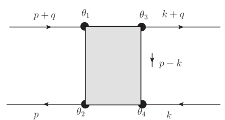
Figure 5: Four point function in superspace

Supersymmetric invariance of the four point function in superspace (3.4) implies that

$$(Q_{\theta_{1},p+q}+Q_{\theta_{2},-p}+Q_{\theta_{3},-k-q}+Q_{\theta_{4},k})V(\theta_{1},\theta_{2},\theta_{3},\theta_{4},p,q,k)=0\ .$$ (417)

This can be simplified using (283) and written as

$$\sum_{i=1}^{4}\bigg{(}\frac{\partial}{\partial\theta_{i}^{\alpha}}-p_{\alpha\beta}(\theta_{1}-\theta_{2})^{\beta}-q_{\alpha\beta}(\theta_{1}-\theta_{3})^{\beta}-k_{\alpha\beta}(\theta_{4}-\theta_{3})^{\beta}\bigg{)}V(\theta_{1},\theta_{2},\theta_{3},p,q,k)=0\ .$$ (418)

We can make the following variable changes to simplify the equation (we suppress spinor indices for simplicity in notation)

$$X=\sum_{i=1}^{4}\theta_{i}\ ,$$

$$X_{12}=\theta_{1}-\theta_{2}\ ,$$

$$X_{13}=\theta_{1}-\theta_{3}\ ,$$

$$X_{43}=\theta_{4}-\theta_{3}\ .$$ (419)

The inverse coordinates are

$$\theta_{1}=\frac{1}{4}(X+X_{12}+2X_{13}-X_{43})\ ,$$

$$\theta_{2}=\frac{1}{4}(X-3X_{12}+2X_{13}-X_{43})\ ,$$

$$\theta_{3}=\frac{1}{4}(X+X_{12}-2X_{13}-X_{43})\ ,$$

$$\theta_{4}=\frac{1}{4}(X+X_{12}-2X_{13}+3X_{43})\ .$$ (420)

In terms of the new coordinates, the derivatives are then expressed as

$$\frac{\partial}{\partial\theta_{1}}=\frac{\partial}{\partial X}+\frac{\partial}{\partial X_{12}}+\frac{\partial}{\partial X_{13}}\ ,$$

$$\frac{\partial}{\partial\theta_{2}}=\frac{\partial}{\partial X}-\frac{\partial}{\partial X_{12}},$$

$$\frac{\partial}{\partial\theta_{3}}=\frac{\partial}{\partial X}-\frac{\partial}{\partial X_{13}}-\frac{\partial}{\partial X_{43}}\ ,$$

$$\sum_{i=1}^{4}\frac{\partial}{\partial\theta_{i}}=4\frac{\partial}{\partial X}\ .$$ (421)

Using the above, one can rewrite (418) as

$$(4\frac{\partial}{\partial X}-p.X_{12}-q.X_{13}-k.X_{43})V(X,X_{12},X_{13},X_{43},p,q,k)=0,$$ (422)

where $p.X_{12}=p_{\alpha\beta}X_{12}^{\beta}$. The above equation can be thought of as a differential equation in the variables $X_{ij}$ and is solved by

$$V(\theta_{1},\theta_{2},\theta_{3},\theta_{4},p,q,k)=\exp\bigg{(}\frac{1}{4}X.(p.X_{12}+q.X_{13}+k.X_{43})\bigg{)}F(X_{12},X_{13},X_{43},p,q,k)\ .$$ (423)

This is the most general form of a four point function in superspace that is invariant under supersymmetry.

H.2 Explicitly evaluating $V_{0}$

In this subsection, we will compute the tree level diagram for the four point function due to the gauge superfield interaction. (see fig 6). In fig 6 the two diagrams are equivalent ways to represent the same process.

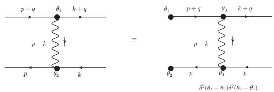
Figure 6: Four point function for gauge interaction: Tree diagram

$$V_{0}(\theta_{1},\theta_{2},\theta_{3},\theta_{4},p,q,k)^{gauge}= \frac{-2\pi}{\kappa(p-k)_{--}}(D_{-}^{\theta_{2},p}-D_{-}^{\theta_{4},k})(D_{-}^{\theta_{1},p+q}-D_{-}^{\theta_{3},-(k+q)})(\delta^{2}_{13}\delta^{2}_{24}\delta^{2}_{12})\ ,$$ (424)

where $\delta_{ij}^{2}=\delta^{2}(\theta_{i}-\theta_{j})$.

It can be explicitly checked that (see (3.4) for definition of $X_{ij}$)

$$(D_{-}^{\theta_{2},p}-D_{-}^{\theta_{4},k})(D_{-}^{\theta_{1},p+q}-D_{-}^{\theta_{3},-(k+q)})(\delta^{2}_{13}\delta^{2}_{24}\delta^{2}_{12})= \exp\bigg{(}\frac{1}{4}X.(p.X_{12}+q.X_{13}+k.X_{43})\bigg{)}$$

$$F_{tree}(X_{12},X_{13},X_{43})\ ,$$ (425)

where

$$F_{tree}=2iX_{12}^{+}X_{13}^{+}X_{43}^{+}(X_{12}^{-}+X_{34}^{-})\ .$$ (426)

Thus the final result for the tree level diagram is given by

$$V_{0}(\theta_{1},\theta_{2},\theta_{3},\theta_{4},p,q,k)^{gauge}= -\frac{4\pi i}{\kappa(p-k)_{--}}\exp\big{(}\frac{1}{4}X_{1234}.(p.X_{12}+q.X_{13}+k.X_{43})\big{)}$$

$$\ X_{12}^{+}X_{13}^{+}X_{43}^{+}(X_{12}^{-}+X_{34}^{-})\ .$$ (427)

It is clear that the shift invariant function (426) has the general structure of (3.5), with the appropriate identification

$$A(p,q,k)=-\frac{4\pi i}{\kappa}\frac{1}{(p-k)_{--}}\ ,\ B(p,q,k)=-\frac{4\pi i}{\kappa}\frac{1}{(p-k)_{--}}$$ (428)

Note that the Fig 6 has the $\mathbb{Z}_{2}$ symmetry (3.4). It is straightforward to check that (H.2) is invariant under (3.4).

H.3 Closure of the ansatz (3.5)

In this section, we establish the consistency of the ansatz (3.5) as a solution of the integral equation (3.5). Consistency is established by plugging the ansatz (3.5) into the RHS of this integral equation, and verifying that the resultant $\theta$ structure is once again of the form given in (3.5). In other words we will show that the dependence of

$$\int\frac{d^{3}r}{(2\pi)^{3}}d^{2}\theta_{a}d^{2}\theta_{b}d^{2}\theta_{A}d^{2}\theta_{B}\bigg{(} NV_{0}(\theta_{1},\theta_{2},\theta_{a},\theta_{b},p,q,r)P(r+q,\theta_{a},\theta_{A})$$

$$P(r,\theta_{B},\theta_{b})V(\theta_{A},\theta_{B},\theta_{3},\theta_{4},r,q,k)\bigg{)}$$ (429)

on $\theta_{1}$, $\theta_{2}$, $\theta_{3}$ and $\theta_{4}$ is given by the form (3.5) with appropriately identified functions $A$, $B$, $C$ $D$.

The algebraic closure described above actually follows from a more general closure property that we now explain. Note that the tree level four point function $V_{0}$ (3.5) is itself of the form (3.5). The more general closure property (which we will explain below) is that the expression

$$V_{12}=V_{1}\star V_{2}\equiv\int\frac{d^{3}r}{(2\pi)^{3}}d^{2}\theta_{a}d^{2}\theta_{b}d^{2}\theta_{A}d^{2}\theta_{B}\bigg{(} V_{1}(\theta_{1},\theta_{2},\theta_{a},\theta_{b},p,q,r)P(r+q,\theta_{a},\theta_{A})$$

$$P(r,\theta_{B},\theta_{b})V_{2}(\theta_{A},\theta_{B},\theta_{3},\theta_{4},r,q,k)\bigg{)}$$ (430)

takes the form (3.5) whenever $V_{1}$ and $V_{2}$ are both also of the form (3.5). In other words (H.3) defines a closed multiplication rule on expressions of the form (3.5).

The explicit verification of the closure described the last paragraph follows from straightforward algebra. Let

$$V_{1}(\theta_{1},\theta_{2},\theta_{a},\theta_{b},p,q,r)=\exp\big{(}\frac{1}{4}X_{12ab}.(p.X_{12}+q.X_{1a}+r.X_{ba})\big{)}F_{1}(X_{12},X_{1a},X_{ba},p,q,r)$$ (431)

where

$$F_{1}(X_{12},X_{1a},X_{ba},p,q,r)=X_{AB}^{+}X_{43}^{+}\bigg{(} A_{1}(p,r,q)X_{12}^{-}X_{ba}^{-}X_{1a}^{+}X_{1a}^{-}+B_{1}(p,r,q)X_{12}^{-}X_{ba}^{-}$$

$$+C_{1}(p,r,q)X_{12}^{-}X_{1a}^{+}+D_{1}(p,r,q)X_{1a}^{+}X_{ba}^{-}\bigg{)}\ .$$ (432)

and

$$V_{2}(\theta_{A},\theta_{B},\theta_{3},\theta_{4},r,q,k)=\exp\big{(}\frac{1}{4}X_{AB34}.(r.X_{AB}+q.X_{A3}+k.X_{43})\big{)}F_{2}(X_{AB},X_{A3},X_{43},r,q,k)\ ,$$ (433)

where

$$F_{2}(X_{AB},X_{A3},X_{43},r,q,k)=X_{AB}^{+}X_{43}^{+}\bigg{(} A_{2}(r,k,q)X_{AB}^{-}X_{43}^{-}X_{A3}^{+}X_{A3}^{-}+B_{2}(r,k,q)X_{AB}^{-}X_{43}^{-}$$

$$+C_{2}(r,k,q)X_{AB}^{-}X_{A3}^{+}+D_{2}(r,k,q)X_{A3}^{+}X_{43}^{-}\bigg{)}\ .$$ (434)

Evaluating the integrals over $\theta_{a},\theta_{b},\theta_{A},\theta_{B}$, we find that $V_{12}$ in (H.3) is of the form (3.5) with

$$A_{12}=-\frac{1}{4}q_{3}\int d^{3}\mathcal{R}\biggl{(} (C_{1}C_{2}k_{-}-D_{1}D_{2}p_{-}+2B_{2}C_{1}q_{3}-2B_{1}D_{2}q_{3})r_{-}$$

$$+2A_{2}(D_{1}p_{-}+2B_{1}q_{3}+2C_{1}r_{-})+2A_{1}(C_{2}k_{-}+2B_{2}q_{3}+2D_{2}r_{-})\biggr{)},$$

$$B_{12}=-\frac{1}{4}\int d^{3}\mathcal{R}\biggl{(} (2A_{2}-C_{2}k_{-})(2A_{1}+D_{1}p_{-})+4B_{1}B_{2}q_{3}^{2}+3C_{1}D_{2}r_{-}^{2}$$

$$+(2A_{2}C_{1}-2A_{1}D_{2}-C_{1}C_{2}k_{-}-D_{1}D_{2}p_{-}+4B_{2}C_{1}q_{3}+4B_{1}D_{2}q_{3})r_{-}\biggr{)},$$

$$C_{12}= -\frac{1}{2}\int d^{3}\mathcal{R}C_{2}q_{3}(2A_{1}+D_{1}p_{-}+2B_{1}q_{3}+3C_{1}r_{-})\ ,$$

$$D_{12}= -\frac{1}{2}\int d^{3}\mathcal{R}D_{1}q_{3}(-2A_{2}+C_{2}k_{-}+2B_{2}q_{3}+3D_{2}r_{-})\ .$$ (435)

where

$$d^{3}\mathcal{R}=\frac{d^{3}r}{(2\pi)^{3}}\frac{1}{(r^{2}+m^{2})((r+q)^{2}+m^{2})}$$

It follows from (H.3) that

$$(V_{1}\star V_{2})\star V_{3}=V_{1}\star(V_{2}\star V_{3})$$ (436)

as both expressions in (436) are given by the same integral (the expressions differ only in the order in which the $\theta$ and internal momentum integrals are performed). In other words the product defined above is associative. We have directly checked that the explicit multiplication formula (H.3) defines an associative product rule.

H.4 Consistency check of the integral equation

In this section, we demonstrate that the integral equations (3.5)-(3.5) are consistent with the $\mathbb{Z}_{2}$ symmetry (3.4). First we note that the $\mathbb{Z}_{2}$ invariance (3.4) of (3.5) imposes the following conditions on the unknown functions of momenta

$$A(p,k,q)=A(k,p,-q)\ ,B(p,k,q)=B(k,p,-q)\ ,$$

$$C(p,k,q)=-D(k,p,-q)\ ,D(p,k,q)=-C(k,p,-q)\ .$$ (437)

These conditions can be written in the form of a matrix given by

$$E(p,k,q)=TE(k,p,-q)\ ,$$ (438)

where

$$T=\left(\begin{array}[]{cccc}1&0&0&0\\ 0&1&0&0\\ 0&0&0&-1\\ 0&0&-1&0\end{array}\right)\ ,E(p,k,q)=\left(\begin{array}[]{c}A\\ B\\ C\\ D\end{array}\right)$$ (447)

The integral equations (3.5)-(3.5) can be written in differential form by taking derivatives of $p_{+}$ and using the formulae in Appendix §H.5

$$\partial_{p_{+}}E(p,k,q)=S(p,k,q)+H(p,k_{-},q)E(p,k,q)\$$ (448)

where $S(p,k,q)$ is a source term. The equation for $k_{+}$ can be obtained from the above equation as follows

$$\partial_{k_{+}}E(p,k,q) =T\partial_{k_{+}}E(k,p,-q)\ ,$$

$$=TS(k,p,-q)+TH(k,p_{-},-q)E(k,p,-q)\ ,$$

$$=TS(k,p,-q)+TH(k,p_{-},-q)TE(p,k,q)\ ,$$ (449)

where we have used (438). Applying $k_{+}$, $p_{+}$ derivative on (448) and (H.4) respectively and taking the difference we get

$$\partial_{k_{+}}S(p,k,q)+H(p,k_{-},q)\bigg{(}TS(k,p,-q)+TH(k,p_{-},-q)TE(p,k,q)\bigg{)}$$

$$=T\partial_{p_{+}}S(k,p,-q)+TH(k,p_{-},-q)T\bigg{(}S(p,k,q)+H(p,k_{-},-q)E(p,k,q)\bigg{)}\ .$$ (450)

Comparing coefficients of $E(p,k,q)$ in the above equation we get the condition

$$[H(p,k_{-},q),TH(k,p_{-},-q)T]=0\ .$$ (451)

For the integral equations (3.5)-(3.5), the $H(p,k_{-},q)$ are given by

$$H(p,k_{-},q_{3})=\frac{1}{a(p_{s},q_{3})}\left(\begin{array}[]{cccc}(6q_{3}-4im)p_{-}&2q_{3}(2im+q_{3})p_{-}&(2im+q_{3})k_{-}p_{-}&-(2im+q_{3})p_{-}^{2}\\ 4p_{-}&4q_{3}p_{-}&-2k_{-}p_{-}&2p_{-}^{2}\\ 0&0&8q_{3}p_{-}&0\\ 8im-4q_{3}&4q_{3}(q_{3}-2im)&2(q_{3}-2im)k_{-}&(4im+6q_{3})p_{-}\\ \end{array}\right)$$ (452)

where

$$a(p_{s},q_{3})=\frac{\sqrt{m^{2}+p_{s}^{2}}\left(4m^{2}+q_{3}^{2}+4p_{s}^{2}\right)}{2\pi}\ .$$ (453)

The matrix $TH(k,p_{,}-q_{3})T$ is

$$TH(k,p_{,}-q_{3})T=\frac{1}{a(k_{s},q_{3})}\left(\begin{array}[]{cccc}-(4im+6q_{3})k_{-}&2q_{3}(q_{3}-2im)k_{-}&-(q_{3}-2im)k_{-}^{2}&(q_{3}-2im)k_{-}p_{-}\\ 4k_{-}&-4q_{3}k_{-}&-2k_{-}^{2}&2k_{-}p_{-}\\ -8im-4q_{3}&4(-2im-q_{3})q_{3}&(4im-6q_{3})k_{-}&-(4im+2q_{3})p_{-}\\ 0&0&0&-8q_{3}k_{-}\\ \end{array}\right)\ ,$$ (454)

It is straightforward to check that (452) and (454) commute. Thus the system of differential equations (448) obey the integrability conditions (451). Thus the differential equations (448) will have solutions that respect the $\mathbb{Z}_{2}$ symmetry.

H.5 Useful formulae

The Euclidean measure for the basic integrals are

$$\int\frac{(d^{3}r)_{E}}{(2\pi)^{3}}=\frac{1}{(2\pi)^{3}}\int r_{s}dr_{s}dr_{3}d\theta\ ,$$ (455)

where $r_{s}^{2}=r_{+}r_{-}=r_{1}^{2}+r_{2}^{2}$ and $r^{2}=r_{s}^{2}+r_{3}^{2}$. Here the integration limits are $-\infty\leq r_{3}\leq\infty$, $0\leq r_{s}\leq\infty$. Most often we encounter integrals of the type,

$$H(q)=\int\frac{d^{3}r}{(2\pi)^{3}}\frac{1}{(r^{2}+m^{2})((r+q)^{2}+m^{2})}=\frac{1}{4\pi|q_{3}|}\tan^{-1}\left(\left|\frac{q_{3}}{2m}\right|\right)$$ (456)

where we have set $q_{\pm}=0$. Another frequently appearing integral is

$$\int\frac{d^{3}r}{(2\pi)^{3}}\frac{1}{r^{2}+m^{2}}=-\frac{|m|}{4\pi}$$ (457)

where we have regulated the divergence using dimensional regularization.

In the integral equations (3.5)-(3.5), there are no explicit functions of $r_{3}$ appearing in the integral equations and the $r_{3}$ integral can be exactly done

$$\int_{-\infty}^{\infty}\frac{dr_{3}}{(r_{s}^{2}+r_{3}^{2}+m^{2})(r_{s}^{2}+(r_{3}+q_{3})^{2}+m^{2})}=\frac{2\pi}{\sqrt{r_{s}^{2}+m^{2}}(4m^{2}+q_{3}^{2}+4r_{s}^{2})}\ .$$ (458)

The results for the angle integrals are

$$\int_{0}^{2\pi}\frac{d\theta}{(r-p)_{-}\ (k-r)_{-}}=\frac{2\pi}{(k-p)_{-}}\bigg{(}\frac{k_{+}}{k_{s}^{2}}\theta[k_{s}-r_{s}]-\frac{p_{+}}{p_{s}^{2}}\theta[p_{s}-r_{s}]\bigg{)}\ ,$$

$$\int_{0}^{2\pi}\frac{d\theta\ r_{-}}{(r-p)_{-}\ (k-r)_{-}}=\frac{2\pi}{(k-p)_{-}}\bigg{(}\theta[k_{s}-r_{s}]-\theta[p_{s}-r_{s}]\bigg{)}\ ,$$

$$\int_{0}^{2\pi}\frac{d\theta\ r_{-}^{2}}{(r-p)_{-}\ (k-r)_{-}}=-\frac{2\pi}{(k-p)_{-}}\bigg{(}k_{-}(1-\theta[k_{s}-r_{s}])-p_{-}(1-\theta[p_{s}-r_{s}])\bigg{)}\ .$$ (459)

while the $r_{s}$ integrals are done with the limits from 0 to $\infty$. We will also make use of the formula

$$\partial_{\bar{z}}\bigg{(}\frac{1}{z}\bigg{)}=2\pi\delta^{2}(z,\bar{z})$$ (460)

to derive the differential form of the integral equations.

For doing the angle integrations in (221) we used the formula (224)

$$\int d\theta{\rm Pv}\cot\left(\frac{\theta}{2}\right){\rm Pv}\cot\left(\frac{\alpha-\theta}{2}\right)=2\pi-4\pi^{2}\delta(\alpha),$$ (461)

where ${\rm Pv}$ stands for principal value. This formula is easily verified by calculating the Fourier coefficients as follows

$$\begin{split}\int\frac{d\alpha}{2\pi}e^{-i\alpha}\int d\theta{\rm Pv}\cot\left(\frac{\theta}{2}\right){\rm Pv}\cot\left(\frac{\alpha-\theta}{2}\right)=&\oint\frac{d\omega}{2\pi\omega}\omega^{-m}\oint\frac{dz}{z}{\rm Pv}\left(\frac{z+1}{z-1}\right){\rm Pv}\left(\frac{z+\omega}{\omega-z}\right)\\ =&\begin{cases}-i\oint dz\,{\rm Pv}\left(\frac{z+1}{z-1}\right)z^{-m-1}=-2\pi&(m>0)\\ 0&(m=0)\\ i\oint dz\,{\rm Pv}\left(\frac{z+1}{z-1}\right)z^{-m-1}=-2\pi&(m<0)\end{cases}\end{split}$$ (462)

where $z=e^{i\theta}$ and $\omega=e^{i\alpha}$. By comparing (462) with Fourier coefficients of delta function,

$$\delta(\alpha)=\frac{1}{2\pi}\sum_{m=-\infty}^{\infty}e^{im\alpha},$$ (463)

we can immediately check (224).

Appendix I Properties of the $J$ functions

The $J$ functions are given by

$$J_{B}(q_{3},\lambda) =\frac{4\pi q_{3}}{\kappa}\frac{n_{1}+n_{2}+n_{3}}{d_{1}+d_{2}+d_{3}}\ ,$$

$$J_{F}(q_{3},\lambda) =\frac{4\pi q_{3}}{\kappa}\frac{-n_{1}+n_{2}+n_{3}}{d_{1}+d_{2}+d_{3}}\ ,$$ (464)

where the parameters are

$$n_{1}= 16mq_{3}(w+1)e^{i\lambda\left(2\tan^{-1}\frac{2|m|}{q_{3}}+\pi\text{sgn}(q_{3})\right)}\ ,$$

$$n_{2}= (w-1)(q_{3}+2im)(2m(w-1)+iq_{3}(w+3))\left(-e^{2i\pi\lambda\text{sgn}(q_{3})}\right)\ ,$$

$$n_{3}= (w-1)(2m+iq_{3})(q_{3}(w+3)+2im(w-1))e^{4i\lambda\tan^{-1}\frac{2|m|}{q_{3}}})\ ,$$

$$d_{1}= (w-1)\left(4m^{2}(w-1)-8imq_{3}+q_{3}^{2}(w+3)\right)e^{4i\lambda\tan^{-1}\frac{2|m|}{q_{3}}}\ ,$$

$$d_{2}= (w-1)\left(4m^{2}(w-1)+8imq_{3}+q_{3}^{2}(w+3)\right)e^{2i\pi\lambda\text{sgn}(q_{3})}\ ,$$

$$d_{3}= -2\left(4m^{2}(w-1)^{2}+q_{3}^{2}(w(w+2)+5)\right)e^{i\lambda\left(2\tan^{-1}\frac{2|m|}{q_{3}}+\pi\text{sgn}(q_{3})\right)}\ .$$ (465)

Both the $J$ functions (I) are even functions of $q_{3}$

$$J_{B}(q_{3},\lambda)=J_{B}(-q_{3},\lambda)\ ,\ J_{F}(q_{3},\lambda)=J_{F}(-q_{3},\lambda)\ .$$ (466)

Therefore in (I) we can replace $q_{3}$ with $|q_{3}|$ and rewrite them as

$$J_{B}(|q_{3}|,\lambda)=\frac{4\pi|q_{3}|}{\kappa}\frac{(\tilde{n}_{1}+\tilde{n}_{2}+\tilde{n}_{3})}{(\tilde{d}_{1}+\tilde{d}_{2}+\tilde{d}_{3})}\ ,$$

$$J_{F}(|q_{3}|,\lambda)=\frac{4\pi|q_{3}|}{\kappa}\frac{(-\tilde{n}_{1}+\tilde{n}_{2}+\tilde{n}_{3})}{(\tilde{d}_{1}+\tilde{d}_{2}+\tilde{d}_{3})}\ ,$$ (467)

where

$$\tilde{n}_{1}= 16m|q_{3}|(w+1)e^{i\lambda\left(2\tan^{-1}\frac{2|m|}{|q_{3}|}+\pi\right)}\ ,$$

$$\tilde{n}_{2}= (w-1)(|q_{3}|+2im)(2m(w-1)+i|q_{3}|(w+3))\left(-e^{2i\pi\lambda}\right)\ ,$$

$$\tilde{n}_{3}= (w-1)(2m+i|q_{3}|)(|q_{3}|(w+3)+2im(w-1))e^{4i\lambda\tan^{-1}\frac{2|m|}{|q_{3}|}})\ ,$$

$$\tilde{d}_{1}= (w-1)\left(4m^{2}(w-1)-8im|q_{3}|+|q_{3}|^{2}(w+3)\right)e^{4i\lambda\tan^{-1}\frac{2|m|}{|q_{3}|}}\ ,$$

$$\tilde{d}_{2}= (w-1)\left(4m^{2}(w-1)+8im|q_{3}|+|q_{3}|^{2}(w+3)\right)e^{2i\pi\lambda}\ ,$$

$$\tilde{d}_{3}= -2\left(4m^{2}(w-1)^{2}+|q_{3}|^{2}(w(w+2)+5)\right)e^{i\lambda\left(2\tan^{-1}\frac{2|m|}{|q_{3}|}+\pi\right)}\ .$$ (468)

Another useful way to write the $J$ function is to use the following identities

$$\tan^{-1}\frac{2m}{q}=\frac{\pi}{2}-\tan^{-1}\frac{q}{2m}$$

$$\tan^{-1}\frac{q}{2m}=\frac{1}{2i}\log\biggl{(}\frac{1+\frac{iq}{2m}}{1-\frac{iq}{2m}}\biggr{)}$$ (469)

Using this relations, it is easy to write the $J$ functions in a factorized form as given in (3.7)

$$J_{B}(q,\lambda)= \frac{4\pi q}{\kappa}\frac{N_{1}N_{2}+M_{1}}{D_{1}D_{2}}\ ,$$

$$J_{F}(q,\lambda)= \frac{4\pi q}{\kappa}\frac{N_{1}N_{2}+M_{2}}{D_{1}D_{2}}\ ,$$ (470)

where

$$N_{1}= \left(\left(\frac{2|m|+iq}{2|m|-iq}\right)^{-\lambda}(w-1)(2m+iq)+(w-1)(2m-iq)\right)\ ,$$

$$N_{2}= \left(\left(\frac{2|m|+iq}{2|m|-iq}\right)^{-\lambda}(q(w+3)+2im(w-1))+(q(w+3)-2im(w-1))\right)\ ,$$

$$M_{1}= -8mq((w+3)(w-1)-4w)\left(\frac{2|m|+iq}{2|m|-iq}\right)^{-\lambda}\ ,$$

$$M_{2}= -8mq(1+w)^{2}\left(\frac{2|m|+iq}{2|m|-iq}\right)^{-\lambda}\ ,$$

$$D_{1}= \left(i\left(\frac{2|m|+iq}{2|m|-iq}\right)^{-\lambda}(w-1)(2m+iq)-2im(w-1)+q(w+3)\right)\ ,$$

$$D_{2}= \left(\left(\frac{2|m|+iq}{2|m|-iq}\right)^{-\lambda}(-q(w+3)-2im(w-1))+(w-1)(q+2im)\right)\ .$$ (471)

Another useful property of the $J$ function is manifest in the above form is its reality under complex conjugation

$$J_{B}(q,\lambda)=J_{B}^{*}(-q,\lambda)\ ,\ J_{F}(q,\lambda)=J_{F}^{*}(-q,\lambda)\ .$$ (472)

Yet another useful way to write the $J$ function is to note that the basic integral which appears in the four point function of scalars in an ungauged theory has the form

$$H(q)=\int\frac{d^{3}r}{(2\pi)^{3}}\frac{1}{(r^{2}+m^{2})((r+q)^{2}+m^{2})}=\frac{1}{4\pi|q_{3}|}\tan^{-1}\left(\left|\frac{q_{3}}{2m}\right|\right)$$ (473)

for $q_{\pm}=0$. Thus we can also write

$$J_{B}(|q|,\lambda)= \frac{4\pi|q|}{\kappa}\frac{N_{1}N_{2}+M_{1}}{D_{1}D_{2}}\ ,$$

$$J_{F}(|q|,\lambda)= \frac{4\pi|q|}{\kappa}\frac{N_{1}N_{2}+M_{2}}{D_{1}D_{2}}\ ,$$ (474)

where

$$N_{1}= \left(e^{-8\pi i\lambda|q|H(q)}(w-1)(2m+i|q|)+(w-1)(2m-i|q|)\right)\ ,$$

$$N_{2}= \left(e^{-8\pi i\lambda|q|H(q)}(|q|(w+3)+2im(w-1))+(|q|(w+3)-2im(w-1))\right)\ ,$$

$$M_{1}= -8m|q|((w+3)(w-1)-4w)e^{-8\pi i\lambda|q|H(q)}\ ,$$

$$M_{2}= -8m|q|(1+w)^{2}e^{-8\pi i\lambda|q|H(q)}\ ,$$

$$D_{1}= \left(ie^{-8\pi i\lambda|q|H(q)}(w-1)(2m+i|q|)-2im(w-1)+|q|(w+3)\right)\ ,$$

$$D_{2}= \left(e^{-8\pi i\lambda|q|H(q)}(-|q|(w+3)-2im(w-1))+(w-1)(|q|+2im)\right)\ .$$ (475)

I.1 Limits of the $J$ function

I.1.1 $\mathcal{N}=2$ point

The $\mathcal{N}=1$ theory studied in this paper enjoys an enhanced $\mathcal{N}=2$ supersymmetry when $w=1$. Naturally in this limit we expect the $J$ functions to have a simplification. In particular we get

$$J_{B}^{w=1}= -\frac{8\pi m}{\kappa}\ ,$$

$$J_{F}^{w=1}= \frac{8\pi m}{\kappa}\ .$$ (476)

I.1.2 Massless limit

There exists a consistent massless limit for the $J$ functions

$$J_{B}^{m=0}=J_{F}^{m=0}=\frac{4\pi|q_{3}|}{\kappa}\frac{(w-1)(w+3)\sin(\pi\lambda)}{(w-1)(w+3)\cos(\pi\lambda)-w(w+2)-5}\ .$$ (477)

This expression is self dual under the duality map (16). Note that when $w=1$ this vanishes and is consistent with the $m\to 0$ limit of (I.1.1).

I.1.3 Non relativistic limit in the singlet channel

The $J$ functions for the S channel are given in (3.10). The non-relativistic limit of the $J$ functions is obtained by taking $\sqrt{s}\to 2m$ with all the other parameters held fixed. In this limit, remarkably we recover the $\mathcal{N}=2$ result.

$$J_{B}^{\sqrt{s}\to 2m}= -\frac{8\pi m}{\kappa}\ ,$$

$$J_{F}^{\sqrt{s}\to 2m}= \frac{8\pi m}{\kappa}\ .$$ (478)

References

- (1) E. Witten, Quantum Field Theory and the Jones Polynomial, Commun.Math.Phys. 121 (1989) 351–399.
- (2) O. Aharony, O. Bergman, and D. L. Jafferis, Fractional M2-branes, JHEP 0811 (2008) 043, [arXiv:0807.4924].
- (3) O. Aharony, O. Bergman, D. L. Jafferis, and J. Maldacena, N=6 superconformal Chern-Simons-matter theories, M2-branes and their gravity duals, JHEP 0810 (2008) 091, [arXiv:0806.1218].
- (4) J. M. Maldacena, The Large N limit of superconformal field theories and supergravity, Int.J.Theor.Phys. 38 (1999) 1113–1133, [hep-th/9711200].
- (5) O. Aharony, S. S. Gubser, J. M. Maldacena, H. Ooguri, and Y. Oz, Large N field theories, string theory and gravity, Phys.Rept. 323 (2000) 183–386, [hep-th/9905111].
- (6) N. Drukker, J. Plefka, and D. Young, Wilson loops in 3-dimensional N=6 supersymmetric Chern-Simons Theory and their string theory duals, JHEP 0811 (2008) 019, [arXiv:0809.2787].
- (7) B. Chen and J.-B. Wu, Supersymmetric Wilson Loops in N=6 Super Chern-Simons-matter theory, Nucl.Phys. B825 (2010) 38–51, [arXiv:0809.2863].
- (8) J. Bhattacharya and S. Minwalla, Superconformal Indices for N = 6 Chern Simons Theories, JHEP 0901 (2009) 014, [arXiv:0806.3251].
- (9) S. Kim, The Complete superconformal index for N=6 Chern-Simons theory, Nucl.Phys. B821 (2009) 241–284, [arXiv:0903.4172].
- (10) A. Kapustin, B. Willett, and I. Yaakov, Exact Results for Wilson Loops in Superconformal Chern-Simons Theories with Matter, JHEP 1003 (2010) 089, [arXiv:0909.4559].
- (11) M. Marino, Lectures on localization and matrix models in supersymmetric Chern-Simons-matter theories, J.Phys. A44 (2011) 463001, [arXiv:1104.0783].
- (12) F. Benini, C. Closset, and S. Cremonesi, Comments on 3d Seiberg-like dualities, JHEP 1110 (2011) 075, [arXiv:1108.5373].
- (13) A. Giveon and D. Kutasov, Seiberg Duality in Chern-Simons Theory, Nucl.Phys. B812 (2009) 1–11, [arXiv:0808.0360].
- (14) A. Agarwal, N. Beisert, and T. McLoughlin, Scattering in Mass-Deformed N¿=4 Chern-Simons Models, JHEP 0906 (2009) 045, [arXiv:0812.3367].
- (15) T. Bargheer, N. Beisert, F. Loebbert, and T. McLoughlin, Conformal Anomaly for Amplitudes in Superconformal Chern-Simons Theory, J.Phys. A45 (2012) 475402, [arXiv:1204.4406].
- (16) M. S. Bianchi, M. Leoni, A. Mauri, S. Penati, and A. Santambrogio, Scattering in ABJ theories, JHEP 1112 (2011) 073, [arXiv:1110.0738].
- (17) W.-M. Chen and Y.-t. Huang, Dualities for Loop Amplitudes of N=6 Chern-Simons Matter Theory, JHEP 1111 (2011) 057, [arXiv:1107.2710].
- (18) M. S. Bianchi, M. Leoni, A. Mauri, S. Penati, and A. Santambrogio, Scattering Amplitudes/Wilson Loop Duality In ABJM Theory, JHEP 1201 (2012) 056, [arXiv:1107.3139].
- (19) M. S. Bianchi and M. Leoni, On the ABJM four-point amplitude at three loops and BDS exponentiation, JHEP 1411 (2014) 077, [arXiv:1403.3398].
- (20) M. S. Bianchi, M. Leoni, A. Mauri, S. Penati, and A. Santambrogio, One Loop Amplitudes In ABJM, JHEP 1207 (2012) 029, [arXiv:1204.4407].
- (21) S. Giombi, S. Minwalla, S. Prakash, S. P. Trivedi, S. R. Wadia, et al., Chern-Simons Theory with Vector Fermion Matter, Eur.Phys.J. C72 (2012) 2112, [arXiv:1110.4386].
- (22) O. Aharony, G. Gur-Ari, and R. Yacoby, d=3 Bosonic Vector Models Coupled to Chern-Simons Gauge Theories, JHEP 1203 (2012) 037, [arXiv:1110.4382].
- (23) J. Maldacena and A. Zhiboedov, Constraining Conformal Field Theories with A Higher Spin Symmetry, J.Phys. A46 (2013) 214011, [arXiv:1112.1016].
- (24) J. Maldacena and A. Zhiboedov, Constraining conformal field theories with a slightly broken higher spin symmetry, Class.Quant.Grav. 30 (2013) 104003, [arXiv:1204.3882].
- (25) C.-M. Chang, S. Minwalla, T. Sharma, and X. Yin, ABJ Triality: from Higher Spin Fields to Strings, J.Phys. A46 (2013) 214009, [arXiv:1207.4485].
- (26) O. Aharony, G. Gur-Ari, and R. Yacoby, Correlation Functions of Large N Chern-Simons-Matter Theories and Bosonization in Three Dimensions, JHEP 1212 (2012) 028, [arXiv:1207.4593].
- (27) S. Jain, S. P. Trivedi, S. R. Wadia, and S. Yokoyama, Supersymmetric Chern-Simons Theories with Vector Matter, JHEP 1210 (2012) 194, [arXiv:1207.4750].
- (28) S. Yokoyama, Chern-Simons-Fermion Vector Model with Chemical Potential, JHEP 1301 (2013) 052, [arXiv:1210.4109].
- (29) G. Gur-Ari and R. Yacoby, Correlators of Large N Fermionic Chern-Simons Vector Models, JHEP 1302 (2013) 150, [arXiv:1211.1866].
- (30) O. Aharony, S. Giombi, G. Gur-Ari, J. Maldacena, and R. Yacoby, The Thermal Free Energy in Large N Chern-Simons-Matter Theories, JHEP 1303 (2013) 121, [arXiv:1211.4843].
- (31) S. Jain, S. Minwalla, T. Sharma, T. Takimi, S. R. Wadia, et al., Phases of large vector Chern-Simons theories on , JHEP 1309 (2013) 009, [arXiv:1301.6169].
- (32) T. Takimi, Duality and higher temperature phases of large N Chern-Simons matter theories on x , JHEP 1307 (2013) 177, [arXiv:1304.3725].
- (33) S. Jain, S. Minwalla, and S. Yokoyama, Chern Simons duality with a fundamental boson and fermion, JHEP 1311 (2013) 037, [arXiv:1305.7235].
- (34) S. Yokoyama, A Note on Large N Thermal Free Energy in Supersymmetric Chern-Simons Vector Models, JHEP 1401 (2014) 148, [arXiv:1310.0902].
- (35) W. A. Bardeen and M. Moshe, Spontaneous breaking of scale invariance in a D=3 U(N ) model with Chern-Simons gauge fields, JHEP 1406 (2014) 113, [arXiv:1402.4196].
- (36) S. Jain, M. Mandlik, S. Minwalla, T. Takimi, S. R. Wadia, et al., Unitarity, Crossing Symmetry and Duality of the S-matrix in large N Chern-Simons theories with fundamental matter, JHEP 1504 (2015) 129, [arXiv:1404.6373].
- (37) W. A. Bardeen, The Massive Fermion Phase for the U(N) Chern-Simons Gauge Theory in D=3 at Large N, JHEP 1410 (2014) 39, [arXiv:1404.7477].
- (38) V. Gurucharan and S. Prakash, Anomalous dimensions in non-supersymmetric bifundamental Chern-Simons theories, JHEP 1409 (2014) 009, [arXiv:1404.7849].
- (39) Y. Dandekar, M. Mandlik, and S. Minwalla, Poles in the -Matrix of Relativistic Chern-Simons Matter theories from Quantum Mechanics, JHEP 1504 (2015) 102, [arXiv:1407.1322].
- (40) Y. Frishman and J. Sonnenschein, Large N Chern-Simons with massive fundamental fermions - A model with no bound states, JHEP 1412 (2014) 165, [arXiv:1409.6083].
- (41) M. Moshe and J. Zinn-Justin, 3D Field Theories with Chern–Simons Term for Large in the Weyl Gauge, JHEP 1501 (2015) 054, [arXiv:1410.0558].
- (42) A. Bedhotiya and S. Prakash, A test of bosonization at the level of four-point functions in Chern-Simons vector models, arXiv:1506.0541.
- (43) G. Gur-Ari and R. Yacoby, Three Dimensional Bosonization From Supersymmetry, arXiv:1507.0437.
- (44) L. Avdeev, D. Kazakov, and I. Kondrashuk, Renormalizations in supersymmetric and nonsupersymmetric nonAbelian Chern-Simons field theories with matter, Nucl.Phys. B391 (1993) 333–357.
- (45) E. Ivanov, Chern-Simons matter systems with manifest N=2 supersymmetry, Phys.Lett. B268 (1991) 203–208.
- (46) D. Gaiotto and X. Yin, Notes on superconformal Chern-Simons-Matter theories, JHEP 0708 (2007) 056, [arXiv:0704.3740].
- (47) G. Amelino-Camelia and D. Bak, Schrodinger selfadjoint extension and quantum field theory, Phys.Lett. B343 (1995) 231–238, [hep-th/9406213].
- (48) S.-J. Kim and C.-k. Lee, Quantum description of anyons: Role of contact terms, Phys.Rev. D55 (1997) 2227–2239, [hep-th/9606054].
- (49) S. Gates, M. T. Grisaru, M. Rocek, and W. Siegel, Superspace Or One Thousand and One Lessons in Supersymmetry, hep-th/0108200.
- (50) T. T. Dumitrescu and N. Seiberg, Supercurrents and Brane Currents in Diverse Dimensions, JHEP 1107 (2011) 095, [arXiv:1106.0031].