Quasi-B-mode generated by high-frequency gravitational waves and corresponding perturbative photon fluxes

Abstract

Interaction of very low-frequency primordial (relic) gravitational waves (GWs)to cosmic microwave background (CMB)can generate B-mode polarization. Here, for the first time we point out that the electromagnetic (EM)response to high-frequency GWs (HFGWs)would produce quasi-B-mode distribution of the perturbative photon fluxes. We study the duality and high complementarity between such two B-modes, and it is shown that such two effects are from the same physical origin: the tensor perturbation of the GWs and not the density perturbation. Based on this quasi-B-mode in HFGWs and related numerical calculation, it is shown that the distinguishing and observing of HFGWs from the braneworld would be quite possible due to their large amplitude, higher frequency and very different physical behaviors between the perturbative photon fluxes and background photons, and the measurement of relic HFGWs may also be possible though face to enormous challenge.

Keywords: High-frequency gravitational waves, Quasi-B-mode, Electromagnetic response, Perturbation photon fluxes.

I Introduction

On 11th Feb 2016 and June 2016, LIGO reported two very important evidencesAbbott et al. (2016a, b) of GW detection. One of them is the GW having amplitude of $h\sim 10^{-21}$ and frequency of $\sim 35$ to $350Hz$. Another one is the GW with amplitude of $h\sim 10^{-22}$ and frequency of $\sim 35$ to $450Hz$, and they are all produced by black hole mergers, which come from distance of 1.3 and 1.4 billion light-years from the Earth, respectively. Obviously, such results are very big encouraging to GW project, and they should push forward research of GW projects, including observation and detection for GWs in different frequency bands, different kinds of GWs, and in different ways. Thus, they should be highly complementary each other.

Before this, in 2014, observation of the B-mode polarization caused by primordial(relic) gravitational waves(GWs) in the cosmic microwave background(CMB) has been reportedAde et al. (2014a). If this B-mode polarization can be completely confirmed by experimental observation, it must also be a great encouragement for detection of GWs in the very-low frequency band, and will provide a key evidence for the inflationary model.
On the other hand, influence of cosmic dusts might swamp the signal of the B-mode polarizationMortonson and Seljak (2014). In addition, if strength of these primordial GWs can reach up to the value reported by the B-mode experiment, then the temperature perturbation induced by the primordial GWs should also be observed, but the Planck satellite did not observe such temperature perturbation. Therefore, further analysis to the B-mode polarization results by data of Planck satellite and other observation ways, will provide critical judgement for the B-mode polarization. However, no matter what the current result is, it should not impact the scheme of observation for B-mode effect caused by the relic GWs, but should strongly attract further attentions of scientific communities on this important phenomenon from the tensor perturbation, and in the future, it would be promising that the research works of B-mode polarization will bring us crucial constraints on the inflationary models.
It should be pointed out that almost all mainstream early universe models and inflation theories predicted primordial (relic) GWs, which have a very broad frequency band distribution. During the very early universe and the inflation epoch of the universe, since extreme small spacetime scale and huge high energy density (they are close to the Planck scale), the quantum effect would play important role and might provide important contribution to generation of the relic gravitons. Then Heisenberg principle would govern the creation and the annihilation of the particles. In this case severe quantum fluctuation would have pumped huge energy into the production of gravitons. In this period, the gravitons having huge energy correspond to extreme-high frequency.
However,the rapid expansion of the universe would have stretched the graviton wavelengths from microscopic to macroscopic length, and present values of these graviton wavelengths would be expected to be from $\sim 1cm$ to the cosmological scale. In other words, the frequency spectrum of the relic GWs would be from $\sim 10^{-17}Hz$ to $\sim 10^{10}Hz$, roughly. Nevertheless, the spectrum densities and dimensionless amplitudes expected by different universe models and scenarios are different due to the different cosmological parameters. Moreover, string theoryGasperini and Veneziano (2003), loop quantum gravityCopeland et al. (2009) and some classical and semi-classical scenariosServin and Brodin (2003); Kogun and Rudenko (2004) also expected the HFGWs, and some of them have interesting and significant strength and properties. Frequency band of the relic GWs predicted by the ordinary inflationary models Grishchuk (2005); Tong and Zhang (2009), the quintessential inflationary modelGiovannini (1999, 2009, 2014) and the pre-big-bang modelGasperini and Veneziano (2003); Veneziano (2004) have been extended to very high frequency range ($\sim 10^{8}~{}to~{}10^{10}~{}Hz$). Moreover, high-frequency GWs(HFGWs) expected by the braneworld senariosClarkson and Seahra (2007) and interaction of astrophysical plasma with intense electromagnetic(EM) radiation from high-energy astrophysical processServin and Brodin (2003) have been extended to $\sim 10^{9}~{}Hz~{}to~{}10^{12}~{}Hz$ or higher frequency, and corresponding dimensionless amplitudes of these HFGWs might reach up to $h\sim 10^{-22}~{}to~{}10^{-27}$(see Table I)Servin and Brodin (2003); Clarkson and Seahra (2007). Besides, even high-energy physics experimentsChen (1994); Wu and Fang (2008)[e.g., see our previous work: Large Hadron Collider(LHC)] also predicted extremely-high frequency GWs(high-energy gravitons)Wu and Fang (2008), and their frequencies might reach up to $10^{19}$ to $10^{23}$ Hz, but the dimensionless amplitude may be only $\sim 10^{-39}$ to $10^{-41}$. Obviously the frequencies of these HFGWs are far beyond the detection or observation range of the intermediate-frequency GWs(e.g., LIGO, GEO600, Virgo, TAMAAbbott et al. (2009a); Seahra et al. (2005); vir ; TAM ; GEO , $\nu\sim 1$ to $10^{4}$Hz), the low-frequency GWs detection(e.g., LISA, BBO, DECIGO….LIS ; Corbin and Cornish (2006); Kawamura et al. (2006), $\nu\sim 10^{-7}$ to $1$Hz),and very low-frequency GWs($\nu\sim 10^{-16}$ to $10^{-17}$Hz, e.g., B-mode experiment in the CMB). Thus, detection and observation of these HFGWs need new principle and scheme. Once the HFGWs can be detectable and observable, then which will open a new information window into the cosmology and the high-energy astrophysical process, and would be highly complementary for the observation of the GWs in the intermediate-, the low-frequency and the very low-frequency bands.

Table 1: Some of possible HFGWs and related properties.

Possible	Ordinary	Quintessential	Pre-big-bang	Brane	Interaction of
HFGWs	inlationaryGrishchuk (2005); Tong and Zhang (2009)	inflationaryGiovannini (1999, 2009, 2014)	Gasperini and Veneziano (2003); Veneziano (2004)	OscillationClarkson and Seahra (2007)	astrophysical plasma
					with intense
					EM radiationServin and Brodin (2003)
Frequency bands	$\sim 10^{8}-10^{10}Hz$	$\sim 10^{9}-10^{10}Hz$	$\sim 10^{9}-10^{10}Hz$	$\sim 10^{8}-10^{14}Hz$	$\sim 10^{9}-10^{12}Hz$
Dimensionless	$\sim 10^{-30}(upper~{}limit)$	$\sim 10^{-30}-10^{-31}$	$\sim 10^{-29}-10^{-31}$	$\sim 10^{-22}-10^{-25}$	$\sim 10^{-25}-10^{-27}$
amplitudes	$-10^{-34}$ or less
	Stochastic	Stochastic	Stochastic	Discrete	Continuous
Properties	background	background	background	spectrum	spectrum

It should be pointed out that the tensor perturbation of GWs is a very common property, which can be not only expressed as B-mode polarizationAde et al. (2014a); Krauss et al. (2010) in the CMB for very low-frequency relic GWs, but also quasi-B-mode distribution of perturbative photon fluxes in electromagnetic response for HFGWs. However, the duality and similarity between the B-mode of the CMB experiment for the very low frequency GWs and the quasi-B-mode of electromagnetic(EM) response for the HFGWs, almost have never been studied in the past. In fact, these effects are all from the same physical origin: tensor perturbation of the GWs and not the density perturbation, and they would be highly complementary , not only in the observable frequency bands, but also in the displaying ways.
In this paper we shall study the similarity and duality between the B-mode polarization in the CMB for very low frequency primordial GWs and the quasi-B-mode distribution of the perturbative photon fluxes(i.e., signal photon fluxes) in the EM response for HFGWs. It is shown that such two B-modes have a fascinating duality and strong complementarity, and distinguishing and observing of the HFGWs expected by the braneworld would be quite possible due to their large amplitude, higher frequency and very different physical behaviors between the perturbative photon fluxes and the background photon fluxes. The measurement of relic HFGWs may also be possible though it face to enormous challenge.
The plan of this paper is follows. In Sec.II we study the strength and angular distribution of the perturbative photon fluxes generated by the HFGWs expected by some typical cosmological models and high-energy astrophysical process, and discuss the duality and similarity between such two B-modes, especially their complementarity due to the same physical reason: the tensor perturbation. In Sec.III we consider displaying conditions for the HFGWs, including the quasi-B-mode experiment in the EM response for the HFGWs. In Sec.IV we discuss wave impedance and wave impedance matching to the perturbative photon fluxes and the background photon fluxes. Our brief conclusion is summarized in Sec.V.

II Quasi-B-mode in electromagnetic response to the high-frequency GWs

It is well known that, “monochromatic components” of the GWs propagating along the z-direction can often be written as Maggiore (2008)

$$h_{\mu\nu}=\left({{\begin{array}[]{*{20}c}0&0&0&0\\ 0&A_{\oplus}&A_{\otimes}&0\\ 0&A_{\otimes}&-A_{\oplus}&0\\ 0&0&0&0\\ \end{array}}}\right)exp[i(k_{g}z-\omega_{g}t)]$$

For the relic GWs, $A_{\oplus}=A(k_{g})/a(t)$, $A_{\otimes}=A(k_{g})/a(t)$, Grishchuk (2005); Tong and Zhang (2009) are the stochastic values of the amplitudes of the relic GWs in the laboratory frame of reference, $\oplus$ and $\otimes$ represent the $\oplus$-type and $\otimes$-type polarizations, and $k_{g}$, $\omega_{g}$ and $a(t)$ are wave vector, angular frequency and the cosmology scale factor in the laboratory frame of reference, respectively. For the non-stochastic coherent GWs, $A_{\oplus}$ and $A_{\otimes}$ are constants.
According to Eq.(II) and electrodynamic equation in curved spacetime, the perturbative EM fields produced by the direct interaction of the incoming GW, Eq.(II), with a static magnetic field $\hat{B}^{(0)}$, can be give byBoccaletti et al. (1970); Li et al. (2008)(we use MKS units)

$${{\tilde{E}_{x}^{(1)}}} = -{\frac{\textit{i}}{2}}A_{\oplus}{{\hat{B}}}^{(0)}k_{g}c\Delta\textit{l}\exp[i(k_{g}z-\omega_{g}t)],$$

$${{\tilde{B}_{y}^{(1)}}} = -{\frac{\textit{i}}{2}}A_{\oplus}{{\hat{B}}}^{(0)}k_{g}\Delta\textit{l}\exp[i(k_{g}z-\omega_{g}t)],$$

$${{\tilde{E}_{y}^{(1)}}} = -{\frac{i}{2}}A_{\otimes}{{\hat{B}}}^{(0)}k_{g}c\Delta l\exp[i(k_{g}z-\omega_{g}t)],$$

$${{\tilde{B}_{x}^{(1)}}} = ~{}~{}\frac{i}{2}A_{\otimes}{{\hat{B}}}^{(0)}k_{g}\Delta l\exp[i(k_{g}z-\omega_{g}t)],$$ (6)

where $\Delta\textit{l}$ is the interaction dimension between the HFGW and the static magnetic field $\hat{B}^{(0)}$, which is perpendicular to the propagating direction of the HFGW, “$\wedge$” stands for the static background magnetic field, “$\sim$” represents time- dependent perturbative EM fields, and the superscript(0) and (1) denote the background and the first-order perturbative EM fields, respectively. Here the perturbative EM fields propagating along the negative z direction(i.e., the opposite propagation direction of the HFGW) are neglected, because they are much weaker or absentBoccaletti et al. (1970); Li et al. (2008); DeLogi and Mickelson (1977). We shall show that using EM synchro-resonance ($\omega_{e}=\omega_{g}$) system of coupling between the static magnetic field $\hat{B}^{(0)}$ and a Gaussian type-photon flux(the Gaussian beam), the “quasi-B-mode” of strength distribution of the perturbative photon flux and the B-mode polarization in the CMB have interesting duality and they would be highly complementary.
According to the quantum electronics, form of the Gaussian-type photon fluxes[the Gaussian beam] is actually expressed by wave beam solution from the Helmholtz equation, and the most basic and general form of the Gaussian beams is the elliptic mode of fundamental frequencyYariv (1989), i.e,

$$\psi = \frac{\psi_{0}\cdot\exp[-(\frac{x^{2}}{W_{x}^{2}}+\frac{y^{2}}{W_{y}^{2}})]}{\sqrt{[1+(z-z_{x})^{2}/f_{x}^{2}]^{\frac{1}{2}}\cdot[1+(z-z_{y})^{2}/f_{y}^{2}]^{\frac{1}{2}}}}$$

$$\cdot \exp\{i[(k_{e}z-\omega_{e}t)-\frac{1}{2}[\tan^{-1}(\frac{z-z_{x}}{f_{x}})+\tan^{-1}(\frac{z-z_{y}}{f_{y}})]+\frac{k_{e}}{2}(\frac{x^{2}}{R_{x}}+\frac{y^{2}}{R_{y}})+\delta]\},$$

where $\psi_{0}$ is the amplitude of the Gaussian beam, $R_{x}=z+f_{x}^{2}/(z-z_{x})$ and $R_{y}=z+f_{y}^{2}/(z-z_{y})$ are the curvature radii of the wave fronts at the xz-plane and at the yz-plane of the Gaussian beam, $f_{x}=\pi W_{0x}^{2}/\lambda_{e}$, $f_{y}=\pi W_{0y}^{2}/\lambda_{e}$, $W_{x}=W_{0x}[1+(z-z_{x})^{2}/f_{x}^{2}]^{\frac{1}{2}}$, $W_{y}=W_{0y}[1+(z-z_{y})^{2}/f_{y}^{2}]^{\frac{1}{2}}$, $W_{0x}$ and $W_{0y}$ are the minimum spot radii of the Gaussian beam at the xz-plane and at the yz-plane, respectively. Here, we shall study case of $R_{x}=R_{y}=R$, $z_{x}=z_{y}=z$, $W_{x}=W_{y}=W$ and $f_{x}=f_{y}=f$, i.e., then the elliptic Gaussian beam, Eq.(II), will be reduced to the circular Gaussian beamYariv (1989).
By using the condition of non-divergence $\nabla\cdot\bf{\tilde{E}}^{(0)}=0$ in free space and $\rm{\bf\tilde{B}^{(0)}}=-i/\omega_{e}\bigtriangledown\times\rm{\bf\tilde{E}^{(0)}}$, we find a group of special wave beam solution of the Gaussian beam as follows:

$${\tilde{E}}_{x}^{(0)}=\psi_{ex} = \psi,{\tilde{E}}_{y}^{(0)}=\psi_{ey}=0,$$

$${\tilde{E}}_{z}^{(0)}=\psi_{ez} = 2x\int(\frac{1}{W^{2}}-i\frac{k_{e}}{2R})\psi dz=2xF(\mathbf{x},k_{e},W),$$

$$F(\mathbf{x},k_{e},W) = \int(\frac{1}{W^{2}}-i\frac{k_{e}}{2R})\psi dz,$$ (8)

$${\tilde{B}}_{x}^{(0)} = \psi_{bx}=-\frac{i}{\omega_{e}}\frac{\partial\psi_{ez}}{\partial y},{\tilde{B}}_{y}^{(0)}=\psi_{by}=-\frac{i}{\omega_{e}}(\frac{\partial\psi}{\partial z}-\frac{\partial\psi_{ez}}{\partial x}),{\tilde{B}}_{z}^{(0)}=\psi_{bz}=\frac{i}{\omega_{e}}\frac{\partial\psi}{\partial y}.$$

Here ${\tilde{B}}_{z}^{(0)}=\psi_{bz}$ is a crucial parameter since the strength and physical behaviour of transverse perturbative photon flux(the transverse signal photon fluxes) mainly depend on ${\tilde{B}}_{z}^{(0)}$[see below and Eqs.(15) to (17)]. Using Eqs.(II) and (II), we have

$${\tilde{B}}_{z}^{(0)}=-[\frac{\psi_{0}k_{e}rsin\phi}{\omega_{e}[1+(z/f)^{2}]^{\frac{1}{2}}(z+f^{2}/z)}+\frac{i2\psi_{0}rsin\phi}{\omega_{e}W_{0}^{2}[1+(z/f)^{2}]^{\frac{3}{2}}}]$$ (10)

$$\cdot \exp(-\frac{r^{2}}{W^{2}})\exp{\{i[(k_{e}z-\omega_{e}t)-\tan^{-1}(\frac{z}{f})+\frac{k_{e}r^{2}}{2R}+\delta]\}}.$$

From Eqs.(II) to (10), we obtain the strength of the transverse background photon fluxes in cylindrical polar coordinates as follows:

$$n_{\phi}^{(0)}=-n_{x}^{(0)}\sin\phi+n_{y}^{(0)}\cos\phi=-\frac{c}{\hbar\omega_{e}}\langle\mathop{T^{01}}\limits^{(0)}\rangle\sin\phi+\frac{c}{\hbar\omega_{e}}\langle\mathop{T^{02}}\limits^{(0)}\rangle\cos\phi$$ (11)

$$= \frac{1}{2\mu_{0}\hbar\omega_{e}}Re\langle\psi_{ez}^{*}\psi_{by}\rangle\sin\phi+\frac{1}{2\mu_{0}\hbar\omega_{e}}Re\langle\psi^{*}\psi_{bz}\rangle\cos\phi$$

$$+ \frac{1}{2\mu_{0}\hbar\omega_{e}}Re\langle\psi_{ez}^{*}\psi_{bx}\rangle\cos\phi=f_{\phi}^{(0)}\exp(-\frac{2r^{2}}{W^{2}})\sin 2\phi,$$

where $\mathop{T^{01}}\limits^{(0)}$ and $\mathop{T^{02}}\limits^{(0)}$ are 01- and 02-components of the energy-momentum tensor for the background EM wave(the Gaussian beam), and

$$n_{x}^{(0)} = \frac{1}{2\mu_{0}\hbar\omega_{e}}Re\langle\psi_{ez}^{*}\psi_{by}\rangle=\frac{1}{2\mu_{0}\hbar\omega_{e}}Re\langle{\tilde{E}}_{z}^{(0)*}{\tilde{B}}_{y}^{(0)}\rangle$$ (12)

$$n_{y}^{(0)} = \frac{1}{2\mu_{0}\hbar\omega_{e}}Re[\langle\psi^{*}\psi_{bz}+\langle\psi_{ez}^{*}\psi_{bx}\rangle]=\frac{1}{2\mu_{0}\hbar\omega_{e}}Re\langle[{\tilde{E}}_{x}^{(0)*}{\tilde{B}}_{z}^{(0)}+{\tilde{E}}_{z}^{(0)*}{\tilde{B}}_{x}^{(0)}]\rangle$$

are the transverse background photon fluxes in the x-direction and in the y-direction, respectively, where $*$ denotes complex conjugate, and the angular brackets represent the average over time, and(also see Ref.Yariv (1989))

$$n_{x}^{(0)}|_{x=0}=n_{y}^{(0)}|_{y=0}=0.$$ (14)

From Eqs.(II) to (14), we obtain the strength distribution of $n_{\phi}^{(0)}$ as follows(see Fig.1)

Figure 1: The strength distribution of background photon flux $n_{\phi}^{(0)}$, Eq.(11), in the cylindrical polar coordinates.

In the same way, under the resonance condition($\omega_{e}=\omega_{g}$), from Eqs.(II),(II),(10), the transverse perturbative photon flux(the signal photon flux) can be given by:

$$n_{\phi}^{(1)}=-n_{x}^{(1)}\sin\phi+n_{y}^{(1)}\cos\phi=-\frac{c}{\hbar\omega_{e}}\langle\mathop{T^{01}}\limits^{(1)}\rangle_{\omega_{e}=\omega_{g}}\sin\phi+\frac{c}{\hbar\omega_{e}}\langle\mathop{T^{02}}\limits^{(1)}\rangle_{\omega_{e}=\omega_{g}}\cos\phi$$ (15)

$$= -\frac{1}{2\mu_{0}\hbar\omega_{e}}Re\langle{\tilde{E}}_{y}^{(1)*}{\tilde{B}}_{z}^{(0)}\rangle_{\omega_{e}=\omega_{g}}\sin\phi+\frac{1}{2\mu_{0}\hbar\omega_{e}}Re\langle{\tilde{E}}_{z}^{(0)*}{\tilde{B}}_{x}^{(1)}\rangle_{\omega_{e}=\omega_{g}}\cos\phi$$

$$+ \frac{1}{2\mu_{0}\hbar\omega_{e}}Re\langle{\tilde{E}}_{x}^{(1)*}{\tilde{B}}_{z}^{(0)}\rangle_{\omega_{e}=\omega_{g}}\cos\phi=n_{\phi-\otimes}^{(1)}+n_{\phi-\otimes}^{(1)^{\prime}}+n^{(1)}_{\phi-\oplus},$$

where $\langle\mathop{T^{01}}\limits^{(1)}\rangle_{\omega_{e}=\omega_{g}}$ and $\langle\mathop{T^{02}}\limits^{(1)}\rangle_{\omega_{e}=\omega_{g}}$ are average values of 01- and 02-components of energy-momentum tensor for first-order perturbation EM fields with respect to time, and

$$n_{\phi-\otimes}^{(1)} = \frac{1}{\mu_{0}\hbar\omega_{e}}\{\frac{A_{\otimes}\hat{B}^{(0)}\psi_{0}k_{g}\Delta\textit{l}r}{2[1+(z/f)^{2}]^{\frac{1}{2}}(z+f^{2}/z)}\sin[\frac{k_{e}r^{2}}{2R}-\tan^{-1}(\frac{z}{f})+\delta]+\frac{A_{\otimes}\hat{B}^{(0)}\psi_{0}\Delta\textit{l}r}{W_{0}^{2}[1+(z/f)^{2}]^{\frac{3}{2}}}$$ (16)

$$\cdot \cos[\frac{k_{e}r^{2}}{2R}-\tan^{-1}(\frac{z}{f})+\delta]\}exp(-\frac{r^{2}}{W^{2}})\sin^{2}\phi,$$

$$n_{\phi-\otimes}^{(1)^{\prime}}=\frac{1}{\mu_{0}\hbar\omega_{e}}\{\frac{1}{2}A_{\otimes}\hat{B}^{(0)}k_{g}\Delta\textit{l}Re\langle F^{*}(\textbf{x},k_{g},W)\cdot exp[i(k_{g}z-\omega_{g}t+\pi/2)]\rangle\}_{\omega_{e}=\omega_{g}}\cos^{2}\phi,~{}~{}~{}$$ (17)

$$n_{\phi-\oplus}^{(1)} = \frac{1}{\mu_{0}\hbar\omega_{e}}\{\frac{A_{\oplus}\hat{B}^{(0)}\psi_{0}k_{g}\Delta\textit{l}r}{4[1+(z/f)^{2}]^{\frac{1}{2}}(z+f^{2}/z)}\sin[\frac{k_{e}r^{2}}{2R}-\tan^{-1}(\frac{z}{f})+\delta]+\frac{A_{\oplus}\hat{B}^{(0)}\psi_{0}\Delta\textit{l}r}{2W_{0}^{2}[1+(z/f)^{2}]^{\frac{3}{2}}}$$ (18)

$$\cdot \cos[\frac{k_{e}r^{2}}{2R}-\tan^{-1}(\frac{z}{f})+\delta]\}exp(-\frac{r^{2}}{W^{2}})\sin 2\phi,$$

where $n_{\phi-\otimes}^{(1)}$ and $n_{\phi-\otimes}^{(1)^{\prime}}$ are the perturbative photon fluxes generated by the $\otimes$-type polarization state of the HFGW, and $n_{\phi-\oplus}^{(1)}$ is the perturbative photon flux produced by the $\oplus$-type polarization state of the HFGW.
It is very interesting to compare the polarization patterns(see Fig.2a) in the CMB caused by primordial density perturbationKrauss et al. (2010) , the polarization patterns(see Fig.2b)Krauss et al. (2010); Ade et al. (2014b) produced by the relic GWs(in the very low frequency band) and the strength distribution(see Fig.2c and 2d) of the perturbative photon fluxes(in the high-frequency band), Eqs.(16) to (17), caused by the HFGWs, respectively.

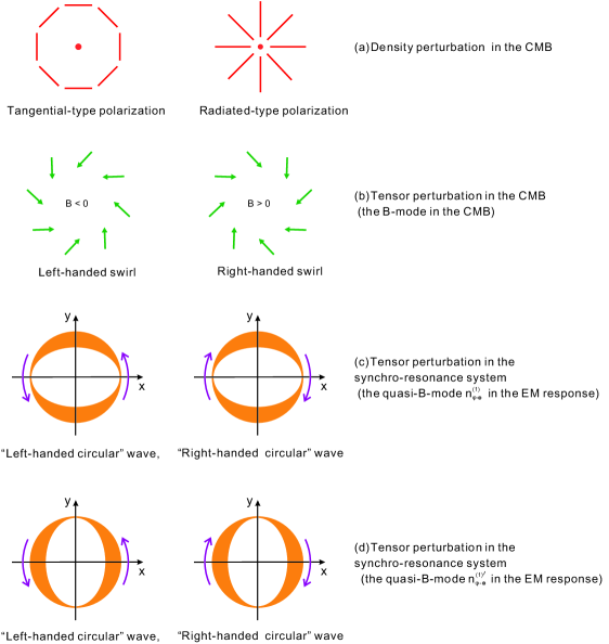
Figure 2: The polarization patterns(Fig.2a) in the CMB caused by primordial density perturbation, the polarization patterns(Fig.2b) in the CMB produced by the relic GWs(tensor perturbation) in very low-frequency band, and the strength distribution(Fig.2c and 2d) of the perturbative photon fluxes in the EM response generated by the HFGWs(tensor perturbation) in the microwave frequency band.

The density perturbation had no right-and-left handed orientation, thus their polarization are expressed as the tangential-type and radiated type patterns. Unlike the density perturbation(Fig.2a), the polarization patterns(Fig.2b) in the CMB produced by the relic GWs are the left-handed and right-handed swirls, and the EM response(Fig.2c and 2d) generated by the HFGWs in our synchro-resonance system are the “left-handed circular wave” and “right-handed circular wave”, the latter both(Fig.2b,2c and 2d) are all from the tensor perturbation of the GWs. Here the “left-handed circular” or the “right-handed circular” property in the EM response depends on the phase factors in Eqs.(16) and (17)(see Fig.3 and below).
By the way, the angular distributions of strength of the perturbative photon flux $n_{\phi-\oplus}^{(1)}$, Eq.(18), and that of the background photon flux $n_{\phi}^{(0)}$, Eq.(11), are the same(Fig.1), i.e., they are not completely “left-handed circular” or completely “right-handed circular”. In this case, $n_{\phi-\oplus}^{(1)}$ will be swamped by $n_{\phi}^{(0)}$. Then, $n_{\phi-\oplus}^{(1)}$ has no observable effect, but $n_{\phi-\otimes}^{(1)}$ and $n_{\phi-\otimes}^{(1)^{\prime}}$ would be observable(see below), and vice versa. Unlike $n_{\phi-\oplus}^{(1)}$, strength of $n_{\phi-\otimes}^{(1)}$, $n_{\phi-\otimes}^{(1)^{\prime}}$ and $n_{\phi}^{(0)}$ have very different physical behaviours, such as different angular distribution and other properties. Eq.(16) shows that $n_{\phi-\otimes}^{(1)}$ has maximum at $\phi=\pi/2$ and $\phi=3\pi/2$(Fig.2c), and $n_{\phi-\otimes}^{(1)^{\prime}}$ has maximum at $\phi=0$ and $\pi$(Fig.2d). This means that the peak value position of the signal photon fluxes are just the zero value areas($\phi=0$, $\pi/2$, $\pi$, $3\pi/2$) of the background photon flux $n_{\phi}^{(0)}$(Fig.1). This is satisfactory. Thus, this novel property would provide an observable effect.

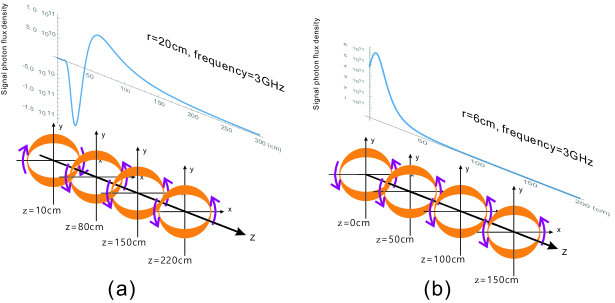
Figure 3: Variation of rotational direction of quasi-B-mode along the propagation direction of HFGW. The $``z^{\prime\prime}$ means the distance to the minimal spot radius of the Gaussian beam, and “r” is the distance to the symmetrical axis of the Gaussian beam.

Analytical expression of the signal photon flux $n_{\phi-\otimes}^{(1)}$, Eq.(16), is a slow enough variational function in the propagating direction z of the HFGW. This means that “rotation direction” of $n_{\phi-\otimes}^{(1)}$ is as slow variational and it remains stable in the almost whole region of coherent resonance. For the HFGW of $\nu=3\times 10^{9}Hz$(i.e., $\lambda_{g}=10cm$), $r=20cm$(distance to the symmetrical axis of Gaussian beam), the “rotation direction” of $n_{\phi-\otimes}^{(1)}$ keeps invariant in the first region of coherent resonance[the coherent resonance region keeping the right-handed rotation, i.e., from $z=10cm$ to $z=40cm$, see the curve in Fig.3(a)], and then, the “rotation direction” will keep invariant in the next region of the coherent resonance[the coherent resonance region always keeping the left-handed rotation, i.e., in the region $z>40cm$[see the curve in Fig.3(a)]. For the case of $r=6cm$[see Fig.3(b)], the rotational direction has a better and more stable physical behavior, i.e., it will always keep left-handed rotational direction in the almost whole coherent resonance region. In other words, the effective receiving area for the HFGW can be $\sim 300~{}cm^{2}$. This means that it has enough large receiving surface to display the perturbative photon flux having $\nu_{g}=3GHz$. Especially, numerical calculation shows that this coherent effective resonance region will be enlarged as the frequency increases, so that the HFGWs having higher frequency will have a larger effective receiving surface(see Fig.4). Fig.4 shows relation between the frequencies of the HFGWs and the effective receiving surface.

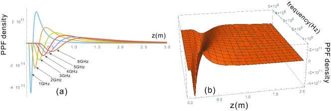
Figure 4: (a)Perturbative photon flux(PPF) density for various frequencies. (b)Relationship between the perturbative photon flux(PPF) density with the frequency and “z”(distance to the minimal spot radius of the Gaussian beam). The curve shows that the “rotation direction” of the perturbative photon flux(PPF) $n_{\phi-\otimes}^{(1)}$ in the EM synchro-resonance system would be more stable for the suitable region, and such distance can be effectively enhanced as the resonance frequency $\nu_{g}$ increases.

Besides, because there are yet other different physical behaviours between the signal photon fluxes $n_{\phi-\otimes}^{(1)}$ and the background photon flux, such as different propagating directions, distribution, decay rates(see, decay factors $exp(-\frac{2r^{2}}{W^{2}})$ of $n_{\phi}^{(0)}$ in Eq.(11) and $exp(-\frac{r^{2}}{W^{2}})$ of $n_{\phi-\otimes}^{(1)}$ in Eqs.(16)), wave impedance(see below), etc in the special local regions, then it is always possible to distinguish the signal photon flux from the noise photons.

III Displaying condition

Since the signal photon fluxes are always accompanied by the noise photons, to identify the total signal photon flux at an effective receiving surface $\Delta S$, $n_{\phi(total)}^{(1)}\Delta t$ must larger than the total noise photon flux fluctuation at the receiving surface $\Delta s$. This displaying condition was discussed in Ref.Li et al. (18v2), we shall not repeat it in detail here, and only give the main numerical calculation results. The displaying condition can be given by:

$$n_{\phi(total)}^{(1)}\Delta t~{}\geq~{}\sqrt{n_{\phi(total)}^{(0)}\Delta t},~{}then~{}\Delta t~{}\geq~{}n_{\phi(total)}^{(0)}/{[n_{\phi(total)}^{(1)}]}^{2}=\Delta t_{min},$$ (19)

where $\Delta t_{min}$ is the requisite minimal accumulation time of the signal, and

$$n_{\phi(total)}^{(1)}=\int\limits_{~{}~{}\Delta s}n_{\phi}^{(1)}ds,~{}n_{\phi(total)}^{(0)}=\int\limits_{~{}~{}\Delta s}n_{\phi}^{(0)}ds,$$ (20)

are the total signal photon flux and the total noise photon flux passing through the receiving surface $\Delta s$, respectively. Actually, there is a narrow frequency distribution of the Gaussian beam, and then the aimed signals caused by HFGWs also should not be monochromatic but with a sensitive frequency range. However, due to this frequency range is very short comparing to the HFGWs frequency band predicted by inflationary models or other scenarios, so we here calculate by a typical representative frequency instead of a frequency window.

Table 2: Displaying condition for the HFGWs in some typical cosmological models and high-energy astrophysical process.

Amplitude(A)	$n_{\phi-\otimes(total)}^{(1)}(s^{-1})$	$\Delta t_{min}(s)$	Allowable upper limit	Possible verifiable cosmological
dimensionless			of noise photon flux$(s^{-1})$	models and astrophysical process
$10^{-23}$	$\sim 1.6\times 10^{9}$	$\sim 10^{4}$	$2.8\times 10^{22}$	Brane oscillationClarkson and Seahra (2007),
$10^{-27}$	$\sim 1.6\times 10^{5}$	$\sim 10^{6}$	$2.8\times 10^{15}$	Interaction of astrophysical plasma
				with intense EM radiationServin and Brodin (2003)
$10^{-30}$	$\sim 1.6\times 10^{2}$	$\sim 10^{6}$	$2.8\times 10^{9}$	Pre-big-bangGasperini and Veneziano (2003); Veneziano (2004),
				Quintessential inflationaryGiovannini (1999, 2009) or
				upper limit of ordinary inflationaryeGrishchuk (2005); Tong and Zhang (2009)

It should be pointed out that the background photon flux(in our synchro-resonance system, typical value of the Gaussian beam is  10W) will be major source to the noise photon flux, i.e., other noise photon fluxes[e.g., shot noise, Johnson noise, quantization noise, thermal noise(if operation temperature $T<1k$), preamplifier noise, diffraction noise, etc.] are all much less than the background photon fluxWoods et al. (2011). In other words, the Gaussian beam(the background photon flux) is likely to the dominant source of noise photons. Moreover, as mentioned earlier, the positions of maximum of the signal photon fluxes( $n_{\phi-\otimes}^{(1)}$ and $n_{\phi-\otimes}^{(1)^{\prime}}$, see Fig.2c and 2d) are just the zero value area of the background photon flux($n_{\phi}^{(0)}$, see Fig.1). Thus, major influence of the noise photon flux at such receiving surfaces would be from the background shot noise photon flux($\sim\sqrt{n_{\phi_{(total)}}^{(0)}}$) and not the background photon flux itself $n_{\phi_{(total)}}^{(0)}$. In this case, the relevant requirements to signal-to-noise ratio can be further relaxed.
Table 2 shows displaying condition of the HFGWs for some cosmological models and high-energy astrophysical process, where $n_{\phi-\otimes(total)}^{(1)}$ are the total signal photon fluxes at the receiving surface $\Delta s$ ($\phi=\pi/2$ or $3\pi/2$ , $\Delta s\sim 3\times 10^{-2}m^{2}$ ), which might be produced by the HFGWs in the Brane oscillation, quintessential inflationary, pre-big-bang models, and the interaction of high-energy plasma with EM radiation, and $n_{total}^{(0)}$ is allowable upper limit of the total noise photon flux at the surface $\Delta s$ for various values of the HFGW amplitudes and $\Delta t_{min}$, Eq.(19), $\nu_{e}=\nu_{g}=3GHz$, the background static magnetic field $B^{(0)}$ is 10T, the interaction dimension $\Delta\textit{l}$ is 2m, the power of the Gaussian beam is $\sim 10W$ and operation temperature should be less than 1K. Fortunately, one of institutes of our research team (High Magnetic Field Laboratory, Chinese Academic of Science) has been fully equipped with the ability to construct the superconducting magnetTan et al. (2009) (this High Magnetic Field Laboratory is also the superconducting magnet builder for the EAST tokamak for controlled nuclear fusion). The magnets can generate a static magnetic field with $\hat{B}^{(0)}=12~{}Tesla$ in an effective cross section of 80cm to 100cm at least, and operation temperature can be reduced to 1K even less. The superconducting static high field magnet will be used for our detection system. Then maximum of $n_{total}^{(0)}$ is $\sim 10^{22}s^{-1}$ at the receiving surface $\Delta s$ of $\phi=\pi/4$, $3\pi/4$, $5\pi/4$ and $7\pi/4$, but it vanishes at $\phi=\pi/2$ and $3\pi/2$(see Fig.1). This means that at such surfaces even if the noise photon flux reach up to the maximum ($\sqrt{n_{total}^{(0)}}\sim 10^{11}s^{-1}$) of the background shot noise photon flux, then $\Delta t_{min}$ can be limited in $\sim 10^{6}~{}seconds$ or less. For the HFGWs in the GHz band expected by the braneworld scenariosClarkson and Seahra (2007), both the maximum $\sqrt{n_{\phi}^{(0)}}|_{max}\sim 10^{11}s^{-1}$ of the background shot noise photon flux or even the maximum($n_{\phi}^{(0)}|_{max}\sim 10^{22}s^{-1}$) of the background photon flux itself are all less or much less than the allowable upper limit($\sim 2.8\times 10^{22}s^{-1}$, see Table 2) of noise photon flux. Thus, direct detection of the HFGWsClarkson and Seahra (2007) in the braneworld scenarios would be quite possible due to larger amplitudes, higher frequencies, discrete spectral nature and extra polarization states for the K-K gravitonsClarkson and Seahra (2007); Nishizawa and Hayama (2013); Wen et al. (2014). Observation of the relic HFGWs predicted by the pre-big-bangGasperini and Veneziano (2003); Veneziano (2004), the quintessential inflationary modelGiovannini (1999, 2009) or the upper limit of the relic HFGWs expected by the ordinary inflationary modelsGrishchuk (2005); Tong and Zhang (2009), will face to enormous challenge, but it is not impossible.

Table 3: The perturbative photon fluxes (PPFs) $n_{\phi(total)}^{(1)}$ and the background photon fluxes (BPFs) $n_{\phi(total)}^{(0)}$ at the receiving $\Delta S$ where $\phi=89^{\circ}$ is azimuth angle in the cylindrical polar coordinates, and r is the distance to the symmetrical axis of the GB. We emphasize again that the important difference among the four main physical behaviors of $n_{\phi(total)}^{(1)}$ and $n_{\phi(total)}^{(0)}$: different angular distribution (see Fig.I and Fig.2(c),(d), the latter are just from the quasi-B-mode), different decay rate (see Eq.(7) and Eq.(12)), very different wave impedance (see Tables IV and V) and different propagation directions in special regions. Importantly, in specific area of the detection system, the propagation direction of $n_{\phi(total)}^{(1)}$ and $n_{\phi(total)}^{(0)}$ are totally inverse each other, so in this case we can observe the signals using highly-oriented photon detector. Thus, only the signals will enter the photon detector and the background noise (of Gaussian Beam) can be effectively depressed. However, some other sources of noise should also be considered. In this table, by acceptable accumulation time of observation, we give the upper limit of these noise such as thermal noise, scattering and diffraction noise, Johnson noise, preamplifier noise and quantization noiseWoods et al. (2011). It was shownWoods et al. (2011) that such noise photon fluxes are less or much less than the upper limit of noise photon fluxes listed in this table.

HFGWE sources	Position of the	$n_{\phi(total)}^{(1)}$	accumulation	upper limit of noise
	receiving surface $\Delta S$ (cm)	$(s^{-1})$	time (s)	photon flux $(s^{-1})$
Brane oscillationClarkson and Seahra (2007)	5cm$<$r$<$10cm	$2.836\times 10^{9}$	$\sim 10^{4}$	$\sim 10^{22}$
	10cm$<$r$<$15cm	$3.235\times 10^{8}$	$\sim 10^{4}$	$\sim 10^{20}$
Quintessential inflationary Giovannini (1999, 2009)
or Pre-big-bangGasperini and Veneziano (2003); Veneziano (2004)	5cm$<$r$<$10cm	283.6	$\sim 10^{4}$	$\sim 10^{8}$

IV Wave impedance and wave impedance matching to the perturbative photon fluxes

The wave impedance to an EM wave(photon flux) depends upon the ratio of the electric component to the magnetic component of the EM wave, and the wave impedance of free space to a planar EM wave is $377\Omega$Haslett (2008), and the wave impedance of copper to EM wave(photon flux) of $\nu=3\times 10^{9}Hz$ is $0.02\Omega$Haslett (2008)(see, Table 3). In fact, the wave impedance to the background photon flux(the Gaussian beam) and the planar EM waves in free space have the same order of magnitude($\sim 377\Omega$). Unlike case of the wave impedance to the background photon flux, the ratio of the electric component of the perturbative photon flux( the signal photon flux) $n_{\phi-\otimes}^{(1)}$, Eq.(16), to its magnetic component in selected wave zone of the synchro-resonance systems is much less than $377\Omega$.

Table 4: The wave impedances to the EM waves(photon fluxes) in different materialsHaslett (2008). This table shows that the wave impedance in the selected wave zone of the synchro-resonance system to the signal photon flux with $\nu_{e}=3\times 10^{9}Hz$, is much less than $0.06\Omega$ of good conductors(e.g., copper), and even smaller than that of superconductor(see below).

Frequency	Wave impedance	Wave impedance	Wave impedance	Wave impedance	Wave impedance
	Copper($\Omega$)	Silver($\Omega$)	Gold($\Omega$)	Superconductor($\Omega$)	Synchro-
					resonance system($\Omega$)
$3\times 10^{9}Hz$	0.060	0.063	0.046	$<10^{-3}$	$\sim 10^{-4}$ or less

Table 5: The wave impedances in the selected wave zone of the synchro-resonance system to the transverse signal photon flux $n^{(1)}_{\phi-\otimes}$ and the background photon flux $n^{(0)}_{\phi}$. Here $\nu_{e}=\nu_{g}=3\times 10^{12}Hz$, $A=10^{-23}$(e.g., the HFGWs in the braneworld modelClarkson and Seahra (2007)) .

Amplitude(A)	Position of	Wave impedance to	Wave impedance to
dimensionless	receiving surface(cm)	perturbative photon flux $n_{\phi-\otimes}^{(1)}(\Omega)$	background photon flux $n_{\phi}^{(0)}(\Omega)$
$10^{-23}$	$x=25,~{}y=5,~{}z=30$	$\sim 3.04\times 10^{-12}$
$10^{-23}$	$x=30,~{}y=5,~{}z=30$	$\sim 6.31\times 10^{-9~{}}$	$\sim 377$
$10^{-23}$	$x=35,~{}y=5,~{}z=30$	$\sim 5.25\times 10^{-5~{}}$
$10^{-23}$	$x=25,~{}y=10,~{}z=30$	$\sim 1.22\times 10^{-11}$
$10^{-23}$	$x=30,~{}y=10,~{}z=30$	$\sim 2.53\times 10^{-8~{}}$	$\sim 377$
$10^{-23}$	$x=35,~{}y=10,~{}z=30$	$\sim 2.11\times 10^{-4~{}}$

It is well known that energy of the electric components are far less than energy of the magnetic components for the EM waves(photon fluxes) propagating in good conductor and superconductorHaslett (2008). This means that the good conductor and superconductor have very low wave impedance, i.e., they have small Ohm losses for such photon fluxes. Then such EM waves(photon fluxes) are easy to propagate and pass through these materials. Fortunately, the signal photon flux in the typical wave zone of our synchro-resonance system has such property, i.e., the ratio of its electric component to the magnetic component is about 5 orders of magnitude less than that of background photon flux and other noise photons at least. This means that the signal photon flux $n_{\phi-\otimes}^{(1)}$ has very small wave impedance(see Table 4), and it would be easier to pass through the transmission way of the synchro-resonance system, i.e., the selected wave zone in the synchro-resonance system would be equivalent to a good “superconductor” to the perturbative photon flux. Contrarily, the wave impedances to the background photon flux and other noise photons, are much greater than the wave impedance to the signal photon flux. I.e., Ohm losses produced by the background photon flux and the other noise photons would be much larger than Ohm losses generated by the signal photon flux in the photon flux receptors and transmission process. Therefore, the signal photon flux could be distinguished from the background photon flux and other noise photons by the wave impedance matching(see Fig.5).
According to definition for the wave impedanceHaslett (2008) and Eqs.(II),(10),(15) and (16), we obtain the wave impedance Z of the typical receiving surface $\Delta s$ to the perturbative photon flux $n_{\phi-\otimes}^{(1)}$ as follows:

$$\mathop{Z}=|\mu_{0}{{\tilde{E}_{y}^{(1)}}}/{\tilde{B}_{z}^{(0)}}|\approx\frac{\mu_{0}A_{\otimes}{{\hat{B}^{(0)}}}\omega_{g}^{2}W^{2}_{0}\Delta l}{4\psi_{0}y}[1+(z/f)^{3/2}]\exp(\frac{r^{2}}{W^{2}}).$$ (21)

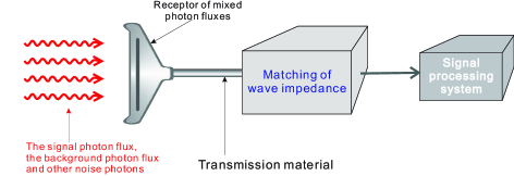
Figure 5: Matching of wave impedance. This figure presents the basic scheme of the matching of wave impedance, to distinguish the signal photon flux from the background noise photon flux. The receptor can collect the mixed photon fluxes(the signal photon and the noise photon fluxes). However, the wave impedance($\sim 10^{-4}\Omega$ or less, see Fig.6, Table 3 and 4) to the signal photon flux $n_{\phi-\otimes}^{(1)}$ is much less than that to the noise photon fluxes(including the background photon flux and other noise photons). The wave impedance matching and the signal processing systems can be only sensitive to the photon fluxes having the low wave impedance and not the photons with high wave impedance. Thus the signal photon flux would be selected and distinguished from the noise photons, due to their very different wave impedances.

By using the typical parameters in the synchro-resonance system and in the typical cosmological models, i.e., $A_{\otimes}\sim 10^{-23}$, $\nu_{g}=3THz$(e.g., the HFGWs in the braneworld modeClarkson and Seahra (2007)), ${\hat{B}^{(0)}}=10T$, $\psi_{0}=2.0\times 10^{3}Vm^{-1}$(for the Gaussian beam of P=10W), $\Delta l=2m$, and selected wave zone: $y\in[5cm,10cm],~{}z\in[0,30cm],~{}x\in[5,30cm]$ for detection: some typical values of the wave impedance we obtained are listed in Table 4 and Fig.6. In the same way it can be shown that there are smaller wave impedance to the signal photon fluxes produced by the HFGWs expected by the pre-big-bang, and quintessential inflationary models(see Fig.6).

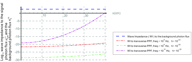
Figure 6: It presents the comparison among wave impedances to the transverse perturbative photon fluxes $n_{\phi-\otimes}^{(1)}$ and to the background photon fluxes having different frequencies and amplitudes in the selected wave zone of the synchro-resonance system. Here x and y are distances to the longitudinal symmetrical surface(the yz-plane and xz-plane) of the Gaussian beam, respectively, and z is distance to the minimum spot radius of the Gaussian beam(see Fig.3), and $y=5cm$, $z=30cm$, $x\in[5,30cm]$. It is clear shown that the wave impedances($\sim 10^{-4}\Omega$ or less) to the transverse perturbative photon flux $n_{\phi-\otimes}^{(1)}$ produced by the HFGW of $h=10^{-23}$, $\nu=3\times 10^{12}Hz$(e.g., the HFGWs in the braneworld modeClarkson and Seahra (2007)), are much less than that of the background photon flux $n^{(0)}_{\phi}$ in such region, and the wave impedances($\sim 10^{-17}\Omega$ or less) to the perturbative photon flux $n_{\phi-\otimes}^{(1)}$ generated by the HFGWs of $h=10^{-30}$, $\nu=3\times 10^{9}Hz$(e.g., the HFGWs in the pre-big-bangGasperini and Veneziano (2003); Veneziano (2004) or in the quintessential inflationary modelGiovannini (1999, 2009), are lot of orders of magnitude lower than that of the background photon flux in the wave zone.

Table 6: Similarity, complementarity and their difference between the two B-modes.

Properties	B-mode in the CMB	Quasi-B-mode in the EM response
Generation mechanism	Interaction of relic GWs with the CMB	EM resonance response to the HFGWs
Physical origin	Tensor perturbation	Tensor perturbation
Effect of available observation	B-mode polarization in the CMB	B-mode distribution of perturbative
		photon fluxes in the EM resonance
Intuitive image	Left-handed and right-handed swirls,	Left-handed and right-handed circular waves
Frequency bands	very-low frequency band	microwave frequency band
	($\sim 10^{-16}~{}to~{}10^{-17}$Hz)	($\sim 10^{9}~{}to~{}10^{12}$Hz)
Type of GWs	Primordial GWs in the	Primordial GWs in the
	very low-frequency band	high-frequency band and other HFGWs
Possible GW sources	Ordinary inflationary and	Quintessential inflationary,
	other possible inflationary	Pre-big-bang,brane oscillation and
		high-energy plasma vibration, etc.
Typical dimension of	Astrophysical scale	Typical laboratory dimension
observation region
Major noise source	The cosmic dusts	The microwave noise photons
		inside the EM resonance system
Wave impedance to signals	$\sim 377\Omega$ (the thermal photon	$\sim 10^{-4}\Omega$ or less (the perturbative
	distribution in the free space)	photon fluxes in the typical wave zone

V Concluding remarks

(i)The B-mode in the CMB is from the interaction of the relic GWs with CMB, and this interaction produces the B-mode polarization in the CMB; the quasi-B-mode in the synchro-resonance system is from EM resonance response to the HFGWs;
(ii)The GW frequencies of the former are located in very low frequency band($\sim 10^{-16}~{}to~{}10^{-17}Hz$), and the GW frequencies of the latter are occurred in typical microwave range($\sim 10^{9}~{}to~{}10^{12}Hz$).
(iii)The B-mode of the former is distributed in astrophysical scale, and the quasi-B-mode of the latter is localized in typical laboratory dimension.
(iv)The major noise source in the former would be from the cosmic dusts, key noise in the latter is from the microwave photons inside the synchro-resonance system, which are almost independent of the cosmic dusts;
(v)Intuitive image of the former are the left-handed swirl and the right-handed swirl in the CMB(Fig.2b), and the physical picture of the latter are expressed as the “left-hand circular wave” and the “right-hand circular wave” distribution of the perturbative photon flux(Fig.2c and 2d);
(vi)The CMB displaying the B-mode are the EM waves(photon fluxes) in the free space, and in fact, it is also a thermal distribution of photons, and typical value of their wave impedance to the B-mode is $\sim 377\Omega$Haslett (2008). Unlike the CMB, the wave impedance($\sim 10^{-4}\Omega$ or less) to the signal photon flux in the typical wave zone of the synchro-resonance system is much less than that of the background photon flux and other noise photons. This means that the perturbative photon flux would be distinguished from the noise photons by the wave impedance matching. The similarity, complementarity and their difference between the two B-modes are listed in Table 6.
Notice, although the above two B-modes correspond to the different situations, their similarity and duality show that they are from the same physical origin: the tensor perturbation of the GWs and not the density perturbation, and only the GWs can generate such similarity and duality, and this is a very important difference to other perturbations and influences.
GWs in ordinary inflation model and the pre-big-bang modelGasperini and Veneziano (2003); Veneziano (2004); Abbott et al. (2009b) involve issues of very early universe and the beginning of time; GWs in the braneworld modelClarkson and Seahra (2007); Seahra et al. (2005) involves issues of the dimension of space, the multiverse, and direction of time arrow; GWs in the quintessential inflationary modelGiovannini (1999, 2009) involve issues of the essence of dark energy, and GWs in high-energy astrophysical processServin and Brodin (2003) involve issues on the interaction mechanism of the interstellar plasma with intense EM radiation. These issues relate to important basic questions: Does the universe have a beginning? If so, how did the universe originate? Was the big-bang the origin of the universe? Was our big-bang the only one? Does the multiverse exist? If so, can it be verified through scientific testing? Would quintessence be a serious candidate for dark energy? Could the interaction between astrophysical plasma and intense EM radiation provide stronger GW sources?
If the GWs are observed in multiple frequency bands in the near future, and not only in the very low-frequency band($\nu\sim 10^{-17}~{}to~{}10^{-16}Hz$), but also in low-frequency band($\nu\sim 10^{-7}$ to $1Hz$), the intermediate-frequency band($\nu\sim 1~{}to~{}10^{4}Hz$) and in the high-frequency band($\nu\sim 10^{8}~{}to~{}10^{12}Hz$), and the observation results have highly self-consistence to the concrete cosmology parameters expected by certain cosmological model or a high-energy astrophysical scenario, then it will provide a stronger evidence for the model or the scenario. If not, the detection sensitivities or observation ways will need further improvement, or these models and scenarios will need to be corrected or will be ruled out.
Finally, it should be pointed out that, the HFGWs can also interact with galactic-extragalactic background magnetic fields, and then lead to EM signals with the same frequency as the HFGWs. Although the galactic-extragalactic background magnetic fields are very weak $\sim 10^{-9}$ to $\sim 10^{-11}$ T, the huge propagation distance could result in a useful spatial accumulation effect in the propagational directionWen et al. (2014), due to the same propagation velocities of HFGWs and EM signals. This may lead to a possibly observable effect on the Earth. Fortunately, such EM signals ($10^{8}$ to $10^{9}$Hz) sit in the detection frequency band of FAST (Five-hundred-meter Aperture Spherical Telescope) which is expected to be completely constructed in 2016 in Guizhou province, China. Therefore, the observation by FAST, detection of the HFGWs by our resonance detection system, and our cooperation with FAST can be strongly complementary. Those consequent works will be carried out in the near future.