Penalty method with P1/P1 finite element approximation for the Stokes equations under slip boundary condition
Abstract.
We consider the P1/P1 or P1b/P1 finite element approximations to the Stokes equations in a bounded smooth domain subject to the slip boundary condition. A penalty method is applied to address the essential boundary condition on , which avoids a variational crime and simultaneously facilitates the numerical implementation. We give -error estimate for velocity and pressure in the energy norm, where and denote the discretization parameter and the penalty parameter, respectively. In the two-dimensional case, it is improved to by applying reduced-order numerical integration to the penalty term. The theoretical results are confirmed by numerical experiments.
Key words and phrases:
Finite element method; Stokes equations; Slip boundary condition; Penalty method; Reduced-order numerical integration2010 Mathematics Subject Classification:
Primary: 65N30; Secondary: 35Q30.1. Introduction
In this paper, letting be a bounded smooth domain, we consider the Stokes equations subject to the non-homogeneous slip boundary condition as follows:
| (1.1) |
where and are the velocity and pressure of the fluid respectively, and is a viscosity constant. Moreover, represents the given body force, the prescribed outgoing flow on the boundary , and the prescribed traction vector on in the tangential direction, with being the Cauchy stress tensor associated with the fluid. The outer unit normal to the boundary is denoted by . The first term in (1.1)1 is added in order to ensure coercivity of the problem without taking into account rigid body movements. We impose the compatibility condition between (1.1)2 and (1.1)3 which reads
| (1.2) |
The slip boundary condition (1.1)3–(1.1)4 (or its variant the Navier boundary condition) is now widely accepted as one of the standard boundary conditions for the Navier-Stokes equations. There are many applications of the slip boundary conditions to real flow problems; here we only mention the coating problem [25] and boundary conditions of high Reynolds number flow [21]. For more details on the application side of slip-type boundary conditions, we refer to Stokes and Carey [27] and references therein; see also John [16] for generalization combined with leak-type boundary conditions.
In the present paper, our motivation to consider problem (1.1) consists in dealing with some mathematical difficulties which are specific to its finite element approximation. As shown by Solonnikov and Ščadilov in [26] (see also Beirão da Veiga [3] for a generalized non-homogeneous problem), proving the existence, uniqueness, and regularity of a solution of (1.1) does not reveal essentially more difficulty compared with the case of Dirichlet boundary conditions. Then one is led to hope that its finite element approximation could also be treated analogously to the Dirichlet case. However, it is known that a naive discretization of (1.1), especially when a smoothly curved domain is approximated by a polyhedral domain , leads to a variational crime in which we no longer obtain convergence of approximate solutions.
Let us describe this phenomenon assuming and considering piecewise linear approximation of velocity. In view of the weak formulation of the continuous problem, see (2.5) below, a natural choice of the space to approximate velocity would be (we adopt the notation of Section 3):
| (1.3) |
where denotes the outer unit normal associated to . Now suppose that and that any two adjacent edges that constitute are not parallel. Then, one readily sees that above reduces to . As a result, the finite element solution computed using is nothing but the one satisfying the Dirichlet boundary condition, which completely fails to approximate the slip boundary condition. For or quadratic approximation (or whatever else), we may well expect similar undesirable reduction in the degrees of freedom that should have been left for the velocity components, which accounts for the variational crime.
One way to overcome the variational crime is to replace the constraint in (1.3) by for each boundary node . This strategy was employed by Tabata and Suzuki [30] where is a spherical shell; see also Tabata [28, 29]. Extension of the idea to the quadratic approximation was proposed by Bänsch and Deckelnick in [1] using some abstract transformation introduced by Lenoir [22]. For of general shape, the exact values for or may not be available. In this regard, some average of ’s near the boundary node can be used as approximation of those unavailable values. This idea was numerically tested by Bänsch and Höhn in [2] for and by Dione, Tibirna and Urquiza [9] for (with penalty formulation), showing good convergence property. However, rigorous and systematic evaluation of those approximations is non-trivial and does not seem to be known in the literature. Moreover, implementation of constraints like in a real finite element code is also non-trivial and requires special computational techniques (see e.g. Gresho and Sani [14, p. 540] and [1, Section 5]), which are not necessary to treat the Dirichlet boundary condition.
In view of these situations, in the present paper we would like to investigate a finite element scheme to (1.1) such that: 1) rigorous error analysis can be performed; 2) numerical implementation is as easy as for the Dirichlet case.
With this aim we adopt a penalty approach proposed by Dione and Urquiza [10] (see also [9]) which, in the continuous setting, replaces the Dirichlet condition (1.1)3 by the Robin-type one involving a very small number (called the penalty parameter) , i.e., on .
At the weak formulation level, this amounts to removing the constraint from the test function space and introducing a penalty term in the weak form.
Our scheme transfers this procedure to the discrete setting given on ; see (3.1) below.
Since the test function space for velocity is taken as the whole involving no constraints, this scheme facilitates implementation, which serves purpose 2) mentioned above.
It is indeed simple enough to be implemented by well-known finite element libraries such as FreeFem++ [15] and FEniCS [23], as is presented in our numerical examples.
Let us turn our attention to the error analysis. The first error estimate was given by Verfürth [31] who derived in the energy norm for . The same author proposed the Lagrange multiplier approach in [32, 33] for . Later, Knobloch [18] derived optimal error estimates (namely, for linear-type approximation and for quadratic-type approximation) for and for various combinations of finite elements satisfying the LBB condition, assuming the existence of better approximation of than . The convergence (without rate) under minimal regularity assumptions was proved by the same author in [19]. A different proof of -estimate for the P2/P1 element was given by [1] for , assuming that is known. The technique using was then exploited to study the penalty scheme in [10], again for the P2/P1 element and for .
In the present paper, we study the penalty scheme for the P1/P1 element combined with pressure stabilization and also for the P1b/P1 element. Our method to establish the error estimate is quite different from those of the preceding works mentioned above. First, we address the non-homogeneous boundary conditions (1.1)3–(1.1)4 which were not considered previously. Second, concerning the penalty scheme, we directly compare and , whereas Dione and Urquiza [10] introduced a penalized problem in the continuous setting, dividing the error estimates into two stages.
Third, we define our error (for velocity) to be , where may be arbitrary smooth extension of . This differs from [32] and [1, 10] in which the errors were defined as and , respectively. In view of practical computation, our choice of the error fits what is usually done in the numerical verification of convergence when . Compared with the method of Knobloch [18] who also employed as the error, the difference lies in the way the boundary element face on is mapped to a part of . In fact, he exploited the orthogonal projection from to , the image of which is localized to each . Then he needed delicate arguments (see [18, pp. 142–143]) to take into account the fact that it is not globally injective when (this point seems to be overlooked in [32, p. 709]). We, to the contrary, rely on the orthogonal projection from to , which is globally bijective regardless of the space dimension , provided the mesh size is sufficiently small. This enables us to transfer the triangulation of to that on in a natural way, which is convenient to estimate surface integrals. Complete proofs of the facts regarding used in this paper, which we could not find in the literature, are provided in Appendices A and B.
Finally, we comment on the rate of convergence we obtain in our main result (Theorem 4.1) which is not optimal. In our opinion, all the error estimates reported in the preceding works, which use to approximate , remain . Verfürth [32, Theorem 5.1] claimed ; however, the estimate
which was used to derive equation (5.12) there, seems non-trivial because is not smooth enough globally on (e.g. it does not belong to ). If on the right-hand side is replaced by , then one ends up with in the final estimate. Dione and Urquiza [10, Theorem 4] claimed ; however, in equation (4.13) there, they did not consider the contribution
which should appear inside the infimum over even when (see Proposition 4.2 of Layton [21]). If this contribution is taken into account, one obtains for the final result.
To overcome the sub-optimality, in Section 5 we investigate the penalty scheme in which reduced-order numerical integration is applied to the penalty term. This method was proposed in [9] and was shown to be efficient by numerical experiments for . We give a rigorous justification for this observation in the sense that the error estimate improves to if . Our numerical example shows that the reduced-order numerical integration gives better results also for , although this is not proved rigorously.
In our numerical results presented in Section 6, we not only provide numerical verification of convergence but also discuss how the penalty parameter affects the performance of linear solvers. We find that too small can lead to non-convergence of iterative methods such as GMRES, whereas sparse direct solvers such as UMFPACK always manage to solve the linear system.
2. Formulation of the Stokes problem with slip boundary condition
We present our notation for the function spaces and bilinear forms that we employ in this paper. The boundary of is supposed to be at least -smooth. The standard Lebesgue and Sobolev(-Slobodetskiĭ) spaces are denoted by and respectively, for and . When , we let . Their vectorial versions are indicated as and etc.; however, in case they appear as subscripts, say , we write for the sake of simplicity. The spaces above may also be defined for ; see e.g. [24].
We define function spaces to describe velocity and pressure as follows:
Also we set
where stands for the trace operator; for simplicity, is indicated as in the following. Finally, to describe a quantity which corresponds to the normal component of the traction vector, i.e. , we introduce
| (2.1) |
where the prime means the dual space.
Let be an open set. The - and -inner products are denoted by and , respectively. Moreover, we define bilinear forms , for , by
| (2.2) | ||||
| (2.3) | ||||
| (2.4) |
where the dot and colon mean the inner products for vectors and matrices, respectively. When , we use the abbreviation . In the following, is also interpreted as the duality pairing between and .
The variational formulation for (1.1) consists in finding such that on and
| (2.5) |
It is well known that this variational equation admits a unique solution under the compatibility condition (1.2) and that it becomes regular according to the smoothness of ; see [3, 26]. Throughout this paper, we assume , so that the regularity is assured.
3. Finite element approximation
3.1. Triangulation and FE spaces
Let us introduce a regular family of triangulations of a polyhedral domain , which is assigned the mesh size . Namely, we assume that:
-
(H1)
each is a closed -simplex such that ;
-
(H2)
;
-
(H3)
the intersection of any two distinct elements is empty or consists of their common face of dimension ;
-
(H4)
there exists a constant , independent of , such that for all where denotes the diameter of the inscribed ball of .
We define the boundary mesh inherited from by
Then we see that satisfies the requirements that are analogous to (H1)–(H4) above, and especially we have . We assume that approximates in the following sense:
-
(H5)
the vertices of every lie on .
Throughout this paper, we confine ourselves to the case where is sufficiently small, which will not be emphasized in the following. In particular, all the results given in Appendices A and B are supposed to hold true.
As mentioned in Section 1, we focus on the P1/P1 and P1b/P1 finite element approximations for velocity and pressure, to which we refer as and , respectively. Namely, we define
where stands for the space spanned by the bubble function on . We also set and . We consider a discrete version of the space (recall (2.1)) as
which is a discontinuous finite element space on .
We turn our attention to interpolation operators. In order to deal with the situation , we first extend functions defined in to , which is a fixed bounded smooth domain containing . For this purpose we consider an arbitrary extension operator satisfying the stability condition
where is a constant depending only on . Such does exist; for example, if we may exploit the zero-extension as , and if it can be constructed e.g. by Nikolskii’s method (see [24]). In view of the lift theorem which concerns a right inverse of the trace operator, we may also extend functions given on to those in . We agree to use the same symbol to refer to this extension as well. Then, given a function in or on , we denote by for simplicity in the notation.
Now we let and represent the Lagrange interpolation operator to linear FE spaces and a local regularization operator to linear FE spaces, respectively. Then, from the theory of interpolation error estimates (see [4, Section 4]) combined with the stability of extension operators, we have
where the constants depend only on , on the constant in assumption (H4) above, and on a reference element. For -estimates, we first apply a trace inequality on each boundary element and then add them up to obtain
3.2. FE scheme with penalty
We propose the following discrete problem to approximate (1.1): choose suitably small and find such that, for all ,
| (3.1) |
where is the outer unit normal of , and (recall (2.2)–(2.4) above). Moreover, represent the extensions of respectively, which are discussed in the previous subsection. is a pressure-stabilizing term, which is present only when and is defined by
We remark that for the case can be any positive constant; here, we suppose it to be for simplicity. We state the well-posedness of this discrete problem.
Proposition 3.1.
There exists a unique solution of (3.1).
The proof relies on the following discrete versions of Korn’s inequality and the inf-sup condition:
| (3.2) | |||||
| (3.3) |
where depends only on and depends only on . Proofs of these uniform coercivity estimates are found in [18, Theorem 4.3] and in [28, Proposition 4], respectively. They will be of central importance when we perform error analysis in Section 4. Now we prove the proposition.
Proof of Proposition 3.1.
We notice that (3.1) is equivalently rewritten as follows: find such that, for all ,
| (3.4) |
Because the problem is finite dimensional, it suffices to prove that for all and implies . Taking yields, thanks to (3.2), and . Below we deal with and separately.
Let . Then, since we have , which implies that equals some constant . By (3.4) one has for all . Choosing such that gives , so that .
3.3. Auxiliary lemmas
We collect several results which will be useful to evaluate the difference of and in terms of volume or surface integrals. We denote the symmetric difference of and by
and call it the boundary skin. The first lemma concerns a linear operator which extends functions in to is equipped with suitable stability properties. For the proof, we refer to [18, Theorem 4.1].
Lemma 3.1.
There exists a linear operator such that and
where the constants are independent of .
The second lemma gives estimates of volume integrals over the boundary skin, which are not restricted to discrete spaces. However, notice that we require higher regularity for the right-hand side.
Lemma 3.2.
Let . Then we have
where is independent of .
Proof.
Lemma 3.3.
Let be the orthogonal projection to defined in a tubular neighborhood of . Then we have the following estimates:
where the constants are independent of . Here, and denote the surface elements associated with and , respectively.
Remark 3.1.
By the first and third estimates together with trace inequalities, for all (hence its extension is in ) we obtain
4. Error analysis of penalty FE scheme
4.1. Estimation of consistency error
To explain the idea, suppose that and that . Then subtracting the discrete problem (3.5) from the continuous one (2.6) would give us
| (4.1) |
This type of relation is essentially important in error analysis of the finite element method and is sometimes called the “Galerkin orthogonality”. If , then such a relation is by no means available because subtraction is impossible. However, even in this case one can still expect that an asymptotic version of (4.1) should hold as becomes small. The next proposition verifies this expectation.
Proposition 4.1.
Proof.
(i) Let us prove (4.2)1. Since , we obtain
| On the other hand, it is clear that | ||||
Addition of the three equations above combined with (2.6)1 and (3.5)1 yields
| (4.3) |
First we estimate volume integrals. It follows from Lemmas 3.1 and 3.2 together with the stability of the extensions that
Next we estimate surface integrals. For we observe that
It follows from Lemma 3.3, Remark 3.1, and Lemma 3.1 that
For we observe that
It follows from Lemmas B.1, 3.3, and 3.1 that
Combining the above estimates with (4.3) and noting that by the regularity theory of the Stokes equations, we conclude (4.2)1.
4.2. Error estimate for velocity and pressure
We are ready to state the main result of this paper.
Theorem 4.1.
Remark 4.1.
As mentioned in Remark 2.1, there is room for us to choose arbitrary additive constant for . Here, we adjust in such a way that , which gives rise to the constant above. By considering instead of , we may assume in the following proof.
Proof of Theorem 4.1.
Let . By interpolation error estimates one has
hence it suffices to bound and by . According to the uniform ellipticity (3.2) we obtain
| (4.4) |
From interpolation error estimates and Proposition 4.1 it follows that
| (4.5) |
For , we observe that
The first three terms are estimated as
whereas we know that by Proposition 4.1. is bounded, thanks to Hölder’s inequality, by
To obtain further estimates of and , we observe from (3.3) that
Here, the second term on the right-hand side is bounded by . We claim that the first term is bounded by . In fact, it follows from (4.2)1, in which is restricted to (hence on so that ), that
This combined with proves the claim. Consequently, we have
| (4.6) |
Collecting the above estimates for and noting that , we deduce
| (4.7) |
In the same way as we computed , one has
By interpolation error estimates on , we have
whereas it follows from (4.2)3 that
Noting that and using Young’s inequality, we arrive at
| (4.8) |
Remark 4.2.
According to the theorem, the best rate of convergence is obtained by choosing , which is not optimal. Let us highlight the reasons for this sub-optimality. First, as far as the variational principle is concerned, the most suitable regularity to work with for would be , instead of as presented above. However, it is not possible to extract this regularity from above (more precisely, in the proof of Proposition 4.1) because . Second, it is not trivial whether the following inf-sup condition would hold:
| (4.9) |
In the case , this condition is valid for a suitable choice of . Çağlar and Liakos [6, 7] took advantage of this fact to derive the optimal rate of convergence .
5. Penalty FE scheme with reduced-order numerical integration
In this section, we investigate problem (3.1) in which is replaced with its reduced-order numerical integration defined via the midpoint (barycenter) formula as follows:
where denotes the area of and is the midpoint of when (resp., the barycenter of when ). Because we exploit pointwise evaluation of functions, we assume higher regularity of the exact solutions as follows:
which implies .
Then the problem we propose reads: find such that
| (5.1) |
for all . The well-posedness of this problem is obtained by the same manner as in Proposition 3.1. We also find that its solution satisfies the following three-variable formulation as we derived (3.5):
where is defined only on by . Likewise, the error analysis is mostly parallel to the arguments in Theorem 4.1. Thereby, in the sequel we only focus on what will change due to the replacement of by . In doing so, first we observe that:
Lemma 5.1.
Let and . Then
Proof.
Since the midpoint (barycenter) formula is exact for affine functions, one obtains
This combined with (note that ) concludes the desired result. ∎
Combining this lemma with the estimates of in the proof of Proposition 4.1, we see that (4.2)1 remains the same even if we replace by .
Next we consider the analysis of (4.2)3, namely, the estimates for – in the proof of Proposition 4.1. To this end we introduce a semi-norm in by
By Lemma B.1 and Cauchy-Schwarz inequality, is bounded by if and by if . By the regularity assumption and by Proposition A.2, we have . We notice that in the present situation is zero. Therefore, instead of (4.2)3 we obtain
| (5.2) |
where if and if .
Finally, we consider the estimates of in the proof of Theorem 4.1. This time we may choose as an interpolation of . In view of the regularity assumption and and by virtue of Lemma B.1, we have
By (5.2), . Consequently, instead of (4.8) we obtain
From these observations, we arrive at the following result.
Theorem 5.1.
Remark 5.1.
According to the theorem, choosing gives us the optimal rate of convergence when . When , at least we see that introduction of reduced-order numerical integration does not deteriorate the rate of convergence. Our numerical example given in the next section shows that it does improve the accuracy for as well.
6. Numerical examples
In the sequel, we refer to the schemes (3.1) and (5.1), i.e. without and with reduced-order numerical integration, as “non-reduced” and “reduced”, respectively.
6.1. Two-dimensional test
In this example, all the computations are done with the use of FreeFem++ [15] choosing the P1/P1 element, i.e. , together with .
Let be the unit disk, namely, .
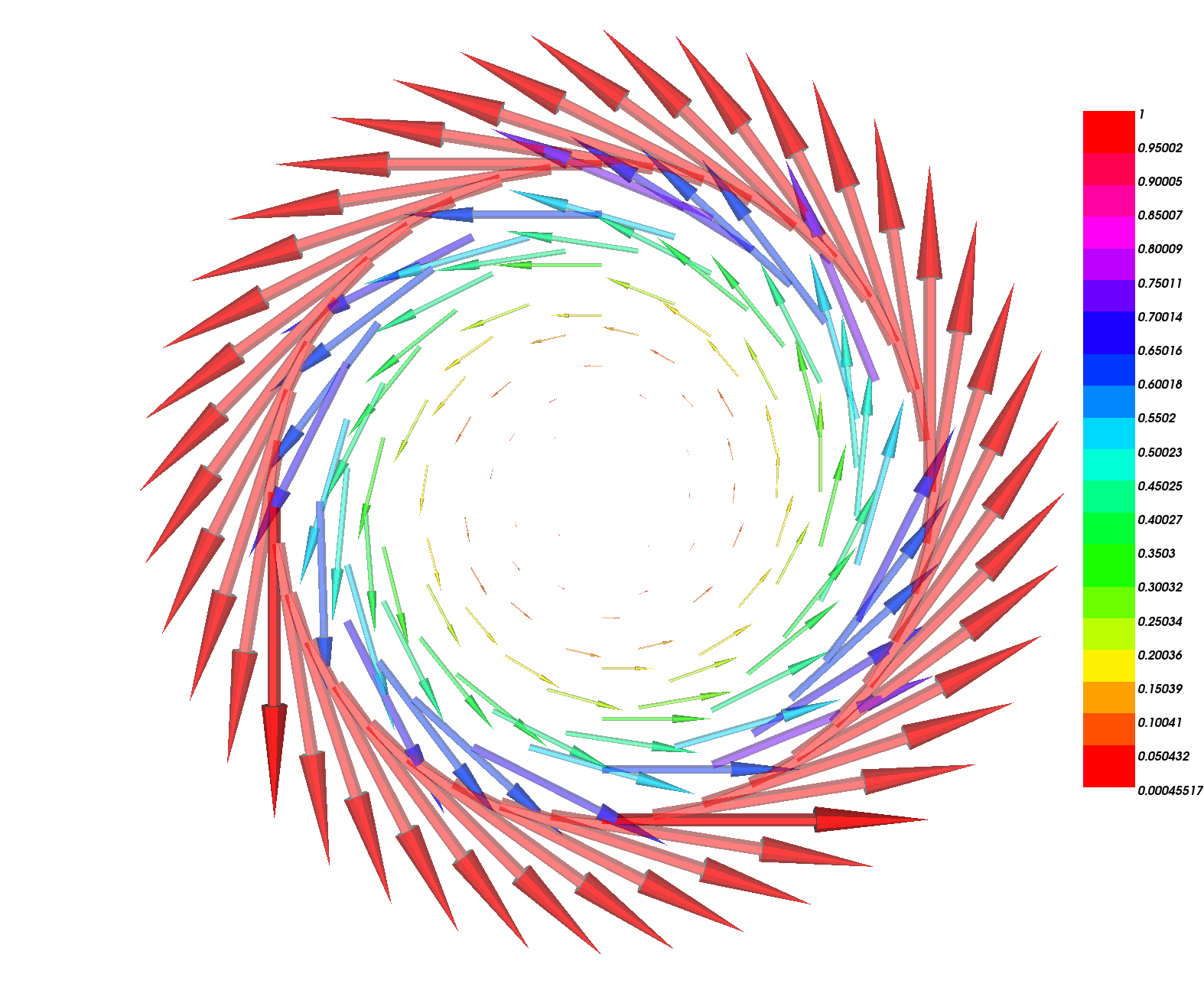
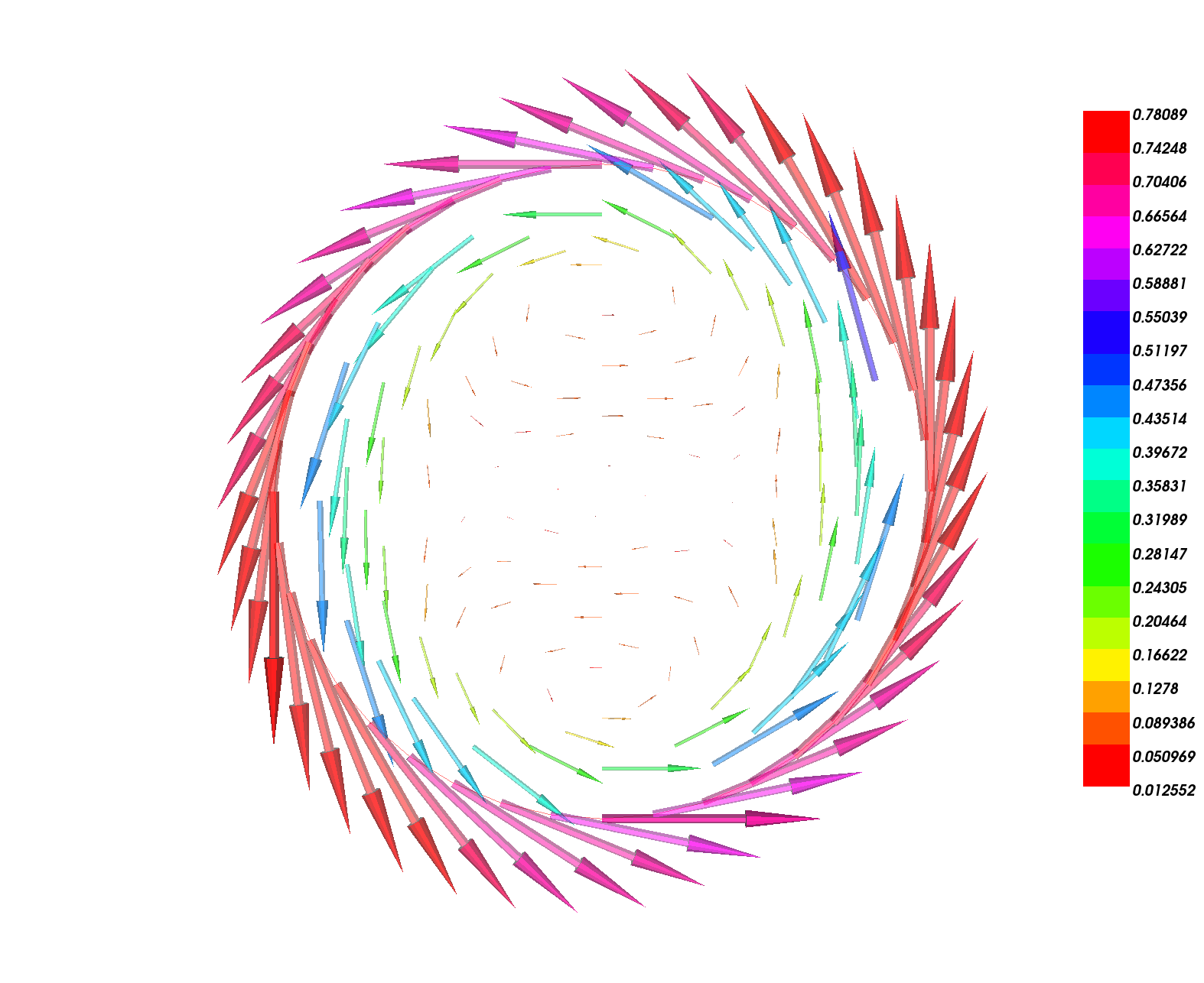
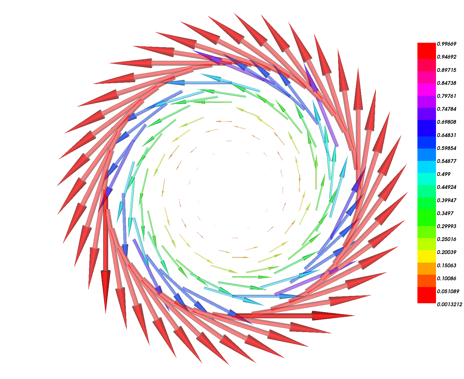
We consider the slip boundary value problem (1.1) for and for given by
in which case we have the analytical solution . We also introduce the solution of the no-slip boundary value problem denoted by . Namely, it is determined according to the same as above and to the boundary condition on . Figure 6.1 shows the velocity profiles of the two solutions; one notices the clear difference in their circulating directions and in the maximum modulus of velocity.


| DOF | Rate | Rate | Rate | ||||
|---|---|---|---|---|---|---|---|
| 0.316 | 333 | 1.043 | — | 0.575 | — | 0.464 | — |
| 0.165 | 1182 | 0.567 | 0.94 | 0.296 | 1.09 | 0.231 | 1.07 |
| 0.078 | 4488 | 0.310 | 0.81 | 0.145 | 0.94 | 0.114 | 0.94 |
| 0.045 | 17391 | 0.146 | 1.37 | 0.077 | 1.30 | 0.057 | 1.28 |
| 0.023 | 69270 | 0.074 | 1.02 | 0.039 | 1.02 | 0.028 | 1.02 |
| 0.012 | 274956 | 0.036 | 1.16 | 0.020 | 1.05 | 0.014 | 1.10 |
| DOF | Rate | Rate | Rate | ||||
|---|---|---|---|---|---|---|---|
| 0.316 | 333 | 1.683 | — | 0.479 | — | 0.464 | — |
| 0.165 | 1182 | 1.559 | 0.12 | 0.232 | 1.12 | 0.231 | 1.07 |
| 0.078 | 4488 | 1.618 | () | 0.114 | 0.95 | 0.114 | 0.94 |
| 0.045 | 17391 | 1.412 | 0.25 | 0.057 | 1.28 | 0.057 | 1.28 |
| 0.023 | 69270 | 1.388 | 0.03 | 0.028 | 1.02 | 0.028 | 1.02 |
| 0.012 | 274956 | 1.293 | 0.11 | 0.014 | 1.10 | 0.014 | 1.10 |
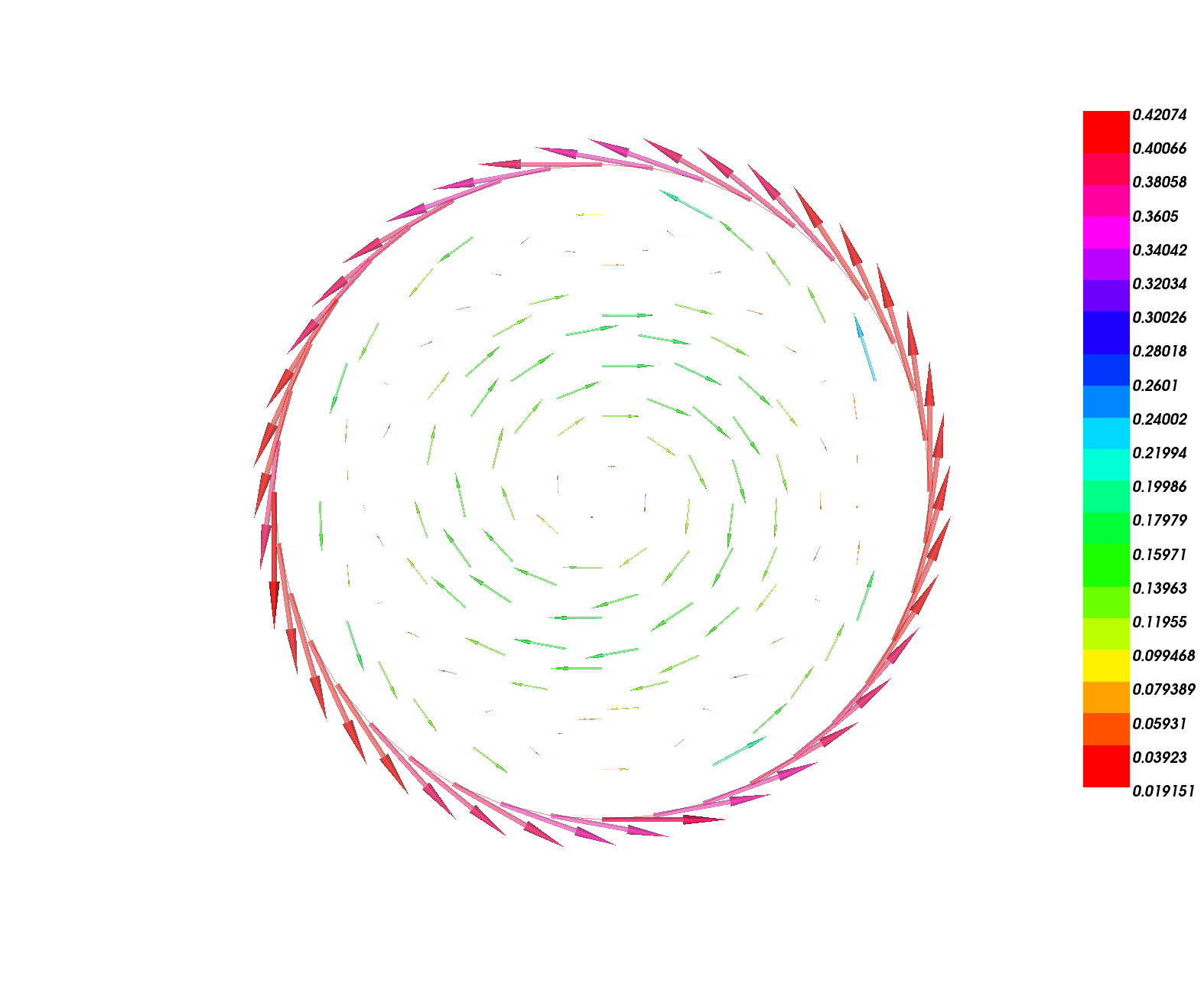
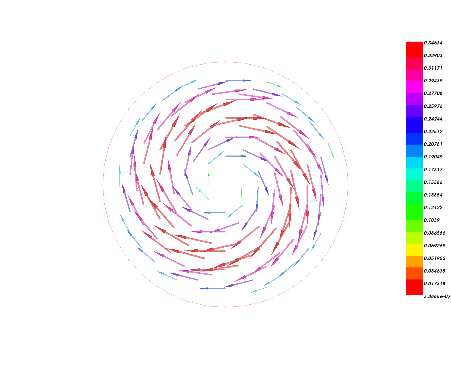
On a mesh with , we computed numerical solutions of the slip boundary value problem using the non-reduced/reduced schemes for three choices of the penalty parameter : , , and very small. The results are shown in Figure 6.2. We find that the reduced scheme gives more robust and accurate approximate solutions. In fact, in case , there are two spurious circulations inside for the non-reduced scheme; we remark that refining a mesh and keeping did not suppress them. For smaller the non-reduced scheme fails to capture the correct solution and seems to approach the no-slip boundary value problem. This behavior is somehow expected because letting in the penalty term of (3.1) implies (at least formally) the constraint on , which undesirably collapses into on as observed in Section 1. However, the reduced scheme produces solutions which capture the slip boundary condition correctly for all sufficiently small. Therefore, it is expected that the error bound (5.3) could be improved in such a way that the reciprocal of would not appear (we conjecture that some inf-sup condition like (4.9) would be valid).
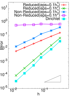
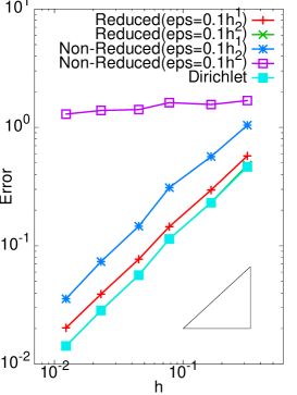
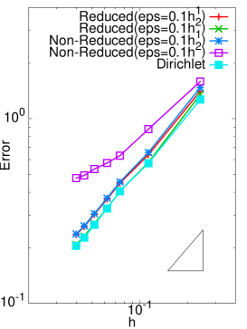
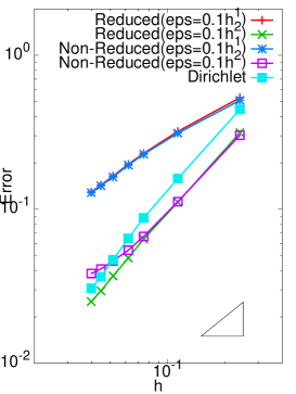
Next we study the convergence property of the non-reduced and reduced schemes, whose solutions are denoted by and , respectively. We compare the convergence behavior of them with that of the numerical solutions computed with the Dirichlet boundary condition, which are denoted by (i.e., the boundary condition on is imposed). The linear solver is chosen as UMFPACK, and and are interpolated into the quadratic finite element space to compute errors in the associated norms. For convenience, we also report errors in the -norm of velocity, and we remark that , , . The results are presented in Table 6.1 and Figure 6.3 for two choices of . We find that for and that for and for , which cannot be explained by the theory. Nevertheless, the fact that the reduced scheme with achieves the best accuracy is in accordance with the theoretical prediction. We see from Figure 6.3 that its accuracy in the energy norm is almost the same as that of .
6.2. Three-dimensional test
In this example, we focus on the verification of convergence. Let be the unit sphere, i.e., . We consider (1.1) for and for such that the analytical solution is
We remark that , , .
The computations are done with the use of FEniCS [23] (combined with Gmsh [12] for obtaining meshes) choosing the P1/P1 element with .
The linear solver is GMRES, preconditioned by incomplete LU factorization, with the restart number 200 and with the relative tolerance .
As in the previous example, and are interpolated into the quadratic finite element space to compute their norms.
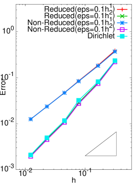
The results are reported in Table 6.2 and Figure 6.4.
Except case of the non-reduced scheme with , the errors seem to converge at the rate , which is better than the theoretically predicted one .
Our opinion is that the interior errors would be dominant with the resolution of meshes considered here and that the suboptimal rate would be observed only for a very fine mesh.
However, from the results we infer that the reduced-order numerical integration is also effective for the case , in which the choice of may be recommended (although this was not justified by a rigorous proof).
With this choice, as in the two-dimensional case, the accuracy in the energy norm is comparable with that of .
| DOF | Rate | Itr | Rate | Itr | Rate | Itr | ||||
|---|---|---|---|---|---|---|---|---|---|---|
| 0.240 | 1.11E+4 | 1.471 | — | 69 | 1.048 | — | 70 | 1.268 | — | 76 |
| 0.113 | 1.12E+5 | 0.656 | 1.08 | 238 | 0.638 | 1.06 | 279 | 0.574 | 1.06 | 349 |
| 0.075 | 3.42E+5 | 0.454 | 0.89 | 352 | 0.448 | 0.86 | 352 | 0.405 | 0.85 | 393 |
| 0.062 | 6.59E+5 | 0.372 | 1.08 | 469 | 0.367 | 1.07 | 473 | 0.326 | 1.16 | 751 |
| 0.052 | 1.17E+6 | 0.306 | 1.05 | 655 | 0.303 | 1.04 | 658 | 0.266 | 1.10 | 790 |
| 0.045 | 1.88E+6 | 0.263 | 1.04 | 901 | 0.261 | 1.03 | 899 | 0.227 | 1.09 | 1979 |
| 0.039 | 2.39E+6 | 0.238 | 0.87 | 1749 | 0.236 | 0.87 | 1638 | 0.205 | 0.88 | 5179 |
| DOF | Rate | Itr | Rate | Itr | Rate | Itr | ||||
|---|---|---|---|---|---|---|---|---|---|---|
| 0.240 | 1.11E+4 | 1.590 | — | 77 | 1.350 | — | 81 | 1.268 | — | 76 |
| 0.113 | 1.12E+5 | 0.877 | 0.79 | 270 | 0.579 | 1.13 | 304 | 0.574 | 1.06 | 349 |
| 0.075 | 3.42E+5 | 0.630 | 0.80 | 467 | 0.405 | 0.87 | 646 | 0.405 | 0.85 | 393 |
| 0.062 | 6.59E+5 | 0.575 | 0.49 | 742 | 0.327 | 1.15 | 782 | 0.326 | 1.16 | 751 |
| 0.052 | 1.17E+6 | 0.534 | 0.41 | 1111 | 0.271 | 1.02 | 1348 | 0.266 | 1.10 | 790 |
| 0.045 | 1.88E+6 | 0.493 | 0.54 | 1735 | 0.231 | 1.08 | 2175 | 0.227 | 1.09 | 1979 |
| 0.039 | 2.39E+6 | 0.477 | 0.29 | 2103 | 0.201 | 0.89 | 2600 | 0.205 | 0.88 | 5179 |

6.3. Affect of penalty parameter on linear solvers
It is known that the use of too strong penalty (i.e. small in our case) would lead to ill-conditioned problems (see e.g. [5]), which could deteriorate the performance of linear solvers.
Therefore, we examine a condition number of the matrix obtained from our penalty FE scheme, in particular, its dependency on the penalty parameter .
For this purpose, we fix the mesh in the 3D test, varying from 100 to .
Moreover, we consider only the reduced scheme since the behavior was similar for the non-reduced one.
The condition number is then estimated by the Matlab function condest(A).
We also report the number of iterations required for GMRES and BiCGSTAB to converge, which were preconditioned by incomplete LU factorization.
The results are presented in Table 6.3.
It seems that the condition number grows at the rate , which is faster than the one explained in [5, p. 532].
One also notices that GMRES and BiCGSTAB failed to converge when .
We remark that, even for such small , sparse direct solvers like UMFPACK or MUMPS were able to solve the linear system (apparently with no problem).
Although we do not have a good explanation of this phenomenon, it tells us that one should carefully choose in order to assure both the accuracy and the numerical stability, especially when one wants to invoke iterative methods for solving linear systems obtained from the penalty method.
| condest(A) | Rate | Itr (restart=30) | Itr (restart=200) | Itr (BiCGSTAB) | |
|---|---|---|---|---|---|
| 1.0E+2 | 2.36E+6 | — | 655 | 182 | 1373 |
| 1.0E+1 | 2.27E+6 | 672 | 191 | 165 | |
| 1.0E+0 | 2.45E+6 | 0.03 | 733 | 195 | 516 |
| 1.0E-1 | 3.53E+6 | 0.16 | 392 | 165 | 264 |
| 1.0E-2 | 1.64E+7 | 0.67 | 480 | 139 | 152 |
| 1.0E-3 | 1.46E+8 | 0.95 | 539 | 195 | 894 |
| 1.0E-4 | 1.56E+9 | 1.03 | 1432 | 352 | 2888 |
| 1.0E-5 | 1.54E+11 | 2.00 | 28162 | 370 | 2293 |
| 1.0E-6 | 1.54E+13 | 2.00 | (not converged) | (not converged) | (not converged) |
| 1.0E-7 | 1.54E+15 | 2.00 | (not converged) | (not converged) | (not converged) |
| 1.0E-8 | 1.54E+17 | 2.00 | (not converged) | (not converged) | (not converged) |
7. Conclusion
We investigated the P1/P1 and P1b/P1 finite element approximations for the Stokes equations subject to the slip boundary condition in a domain with a smooth boundary. The constraint on is relaxed by using the penalty method, which enables us to avoid a variational crime and makes the numerical implementation easier. We developed a framework to address the difficulty due to and successfully applied it to establish error estimates of the finite element approximation. The use of reduced-order numerical integration together with in the penalty term improves the accuracy, which was theoretically justified for and was numerically confirmed for . In fact, we observed that the accuracy in the energy norm was comparable with that of numerical solutions subject to Dirichlet boundary conditions.
Appendix A Transformation between and and related estimates
Let be a bounded domain in . Its boundary is assumed to be -smooth, namely, there exist a system of local coordinates and positive numbers such that: 1) forms an open covering of ; 2) is a rotated coordinate of the original one , that is, for some orthogonal transformation ; 3) gives a graph representation of , where , that is,
Since is compact, there exists such that for any the open ball is contained in some local coordinate neighborhood . According to the fact that , the derivatives of are bounded up to second order, i.e.,
where are constants independent of , and means .
The smoothness of is connected with that of the signed distance function defined by
We collect several known properties on below. For the details, see e.g. [13, Section 14.6] or [8, Section 7.8]. Let be a tubular neighborhood of with width . Then there exists depending only on the curvature of such that for arbitrary the decomposition
| (A.1) |
is uniquely determined. Here, is the outer unit normal field defined on , which coincides with . We extend from to by , which also agrees with . The fact that is -smooth implies that , , and . We call the orthogonal projection onto , in view of its geometrical meaning. We may assume that
where we re-choose the constants if necessary.
Now we introduce a regular family of triangulations of in the sense of Section 3.1. As before, we denote by the boundary mesh inherited from , and we set and . In order for to be compatible with the local-coordinate system , we assume the following:
-
1)
the mesh size is less than ;
-
2)
for every , is represented by a graph ;
-
3)
every vertex of lies on .
From these we see that every is contained in some and that is a piecewise linear interpolation of . As a result of interpolation error estimates, for arbitrary we obtain
where we re-choose if necessary and the subscript E refers to “error”. In the following, is made small enough to satisfy , which in particular ensures that is well-defined on . We may assume further that is contained in the same that contains .
Based on the observations above, we see that the orthogonal projection maps into . It indeed gives a homeomorphism between and , and is element-wisely a diffeomorphism, as shown below. The representation of a function in each local coordinate is defined as . However, with some abuse of notation, we denote it simply by . Then, the local representation of the outer unit normal associated to is given by
where . We are ready to state the following.
Proposition A.1.
If is sufficiently small, then is a homeomorphism between and .
Proof.
Let us construct an inverse map of which is continuous. To this end, we fix arbitrary and choose a local coordinate of such that . For simplicity, we omit the subscript in the following. In view of the definition of by (A.1), we introduce a segment given by
To each point on this segment we associate its height with respect to the graph of , that is,
Then we assert that and that , .
To prove the first assertion, letting
we have . One sees that
where and satisfy
Then it follows that
From this we have provided . For the second assertion, one finds that
where is . By Taylor’s theorem, there exists some such that
By the definition of and by , we obtain
which implies that provided . In the same way, the last assertion can be proved.
From these assertions we deduce that there exists a unique such that . Consequently, the map is well-defined. A direct computation combined with the uniqueness of the decomposition (A.1) shows that is the inverse of . The continuity of , especially that of , follows from an argument similar to the proof of the implicit function theorem (see e.g. [20, Theorem 3.2.1]). ∎
Proposition A.1 enables us to define an exact triangulation of by
In particular, we can subdivide into disjoint sets as . Furthermore, for each we see that and admit the same domain of parametrization, which is important in the subsequent analysis. To describe this fact, we choose a local coordinate such that , and introduce the projection to the base set by . The domain of parametrization is then defined to be . We observe that the mappings
are bijective and that is smooth on . If in addition , especially , is also smooth on , then and may be employed as smooth parametrizations for and respectively. The next proposition verifies that this is indeed the case.
Proposition A.2.
Under the setting above, we have
where and are constants depending only on and .
Proof.
Since the first relation is already obtained in Proposition A.1 with , we focus on proving the second one. For notational simplicity, we omit the subscript and also use the abbreviation . The fact that is differentiable with respect to can be shown in a way similar to the proof of the implicit function theorem. Thereby it remains to evaluate the supremum norm of in , which we address in the following.
Recall that is determined according to the equation
| (A.2) |
where we have set . Because , it follows that
Therefore, it suffices to prove that ; here and hereafter denotes various constants which depends only on and .
Remark A.1.
Let . Since is linear on , further differentiation of (A.3) gives us ; in fact we have . This implies that is a -diffeomorphism between and . However, since is smooth only within , is not globally a diffeomorphism.
Now we give an error estimate for surface integrals on and . Heuristically speaking, the result reads , which may be found in the literature (see e.g. [11]). Here and hereafter, we denote the surface elements of and by and , respectively.
Theorem A.1.
Let and be an integrable function on . Then we have
where is a constant depending only on and .
Proof.
Let be a local coordinate that contains . We omit the subscript and use the abbreviation . We represent the surface integral using the parametrization as follows:
where denotes the Riemannian metric tensor given by (dot means the inner product in ). Similarly, noting that , one obtains
where is given by . Then we assert that:
To prove this, noting that , we compute each component of as follows:
For , we notice that is a tangent vector so that . This yields
which is estimated by thanks to Proposition A.2. can be bounded in the same manner. To estimate , we observe that
which is bounded by . Similarly one gets , hence it follows that . Therefore, , which proves the assertion.
Now we use the following crude estimate for perturbation of determinants (cf. [17, equation (3.13)]): if and are matrices such that and for all , then
Combining this with the assertion above and also with , we obtain
In addition, note that . Consequently,
which proves the theorem. ∎
Remark A.2.
Adding up the results of the theorem for all yields
It also follows that . Choosing in particular as the integrand gives for .
Let be a smooth function given on . Then its transformation to is defined by . However, if is extended to a neighborhood of , e.g. to , then we may also consider ’s natural trace on . The next theorem provides error estimation of these two quantities.
Theorem A.2.
Let , where and . Then,
where is a constant depending only on .
Proof.
Since , where denotes a tubular neighborhood of , it suffices to prove that
| (A.4) |
To this end, using the notation in Theorem A.1, we estimate the left-hand side of (A.4) by
Here, for fixed we have
Because , it follows that
where we have used Hölder’s inequality. Consequently,
| (A.5) |
On the other hand, we observe that the -dimensional transformation
| (A.6) |
is bijective and smooth. Application of this transformation to the right-hand side of (A.4) leads to
where denotes the Jacobi matrix of . Letting , we find that
because . This implies
which combined with yields if is sufficiently small. Therefore,
| (A.7) |
The desired estimate (A.4) is now a consequence of (A.5) and (A.7). This completes the proof. ∎
Finally, we show that the -norm in a tubular neighborhood can be bounded in terms of its width. Such estimate is stated e.g. in [35, Lemma 2.1] or in [28, equation (3.6)]. However, since we could not find a full proof of this fact (especially for ) in the literature, we present it here.
Theorem A.3.
Proof.
We adopt the same notation as in the proofs of Theorems A.1 and A.2. Then it suffices to prove that
To this end, using the transformation given in (A.6) we express the left-hand side as
For , we see from the same argument as before that
which yields
For , it follows that
We have thus obtained the desired estimate, which completes the proof. ∎
Appendix B Error of and
Let us prove that on and also that, when , it is improved to if the consideration is restricted to the midpoint of edges.
Lemma B.1.
Let and be the outer unit normals to and respectively. Then there holds
| (B.1) |
If in addition , , and denotes the midpoint of , then
| (B.2) |
Here, is a constant depending only on and .
Proof.
Let be arbitrary and let be a local coordinate that contains . We omit the subscript in the following. One sees that and are represented as
A direct computation gives
| (B.3) |
This combined with the observation that
proves (B.1). When and , by using Taylor expansion, we find that is a point of super-convergence such that . This improves (B.3) to , and thus (B.2) is proved. ∎
Acknowledgements
The authors thank Professor Fumio Kikuchi, Professor Norikazu Saito, and Professor Masahisa Tabata for valuable comments to the results of this paper. They also thank Professor Xuefeng Liu for giving them a program which converts matrices described by the PETSc-format into those by the CRS-format. The first author was supported by JST, CREST. The second author was supported by JSPS KAKENHI Grant Number 24224004, 26800089. The third author was supported by JST, CREST and by JSPS KAKENHI Grant Number 23340023.
References
- [1] E. Bänsch and K. Deckelnick, Optimal error estimates for the Stokes and Navier-Stokes equations with slip-boundary condition, Math. Mod. Numer. Anal., 33 (1999), pp. 923–938.
- [2] E. Bänsch and B. Höhn, Numerical treatment of the Navier-Stokes equations with slip boundary condition, SIAM J. Sci. Comput., 21 (2000), pp. 2144–2162.
- [3] H. Beirão da Veiga, Regularity for Stokes and generalized Stokes systems under nonhomogeneous slip-type boundary conditions, Adv. Differential Equations, 9 (2004), pp. 1079–1114.
- [4] S. C. Brenner and L. R. Scott, The Mathematical Theory of Finite Element Methods, Springer, 3rd ed., 2007.
- [5] P. Castillo, Performance of discontinuous Galerkin methods for elliptic PDEs, SIAM J. Sci. Comput., 24 (2002), pp. 524–547.
- [6] A. Çağlar, Weak imposition of boundary conditions for the Navier-Stokes equations, Appl. Math. Comput., 149 (2004), pp. 119–145.
- [7] A. Çağlar and A. Liakos, Weak imposition of boundary conditions for the Navier-Stokes equations by a penalty method, Int. J. Numer. Meth. Fluids, 61 (2009), pp. 411–431.
- [8] M. C. Delfour and J.-P. Zolésio, Shapes and Geometries—Metrics, Analysis, Differential Calculus, and Optimization, SIAM, 2nd ed., 2011.
- [9] I. Dione, C. Tibirna, and J. Urquiza, Stokes equations with penalised slip boundary conditions, Int. J. Comput. Fluid Dyn., 27 (2013), pp. 283–296.
- [10] I. Dione and J. Urquiza, Penalty: finite element approximation of Stokes equations with slip boundary conditions, Numer. Math., doi: 10.1007/s0021-014-0646-9 (published online).
- [11] G. Dziuk, Finite elements for the Beltrami operator on arbitrary surfaces, Lecture Notes in Math., 1357 (1988), pp. 142–155.
- [12] C. Geuzaine and J.-F. Remacle, Gmsh: a three-dimensional finite element mesh generator with built-in pre- and post-processing facilities, Int. J. Numer. Meth. Eng., 79 (2009), pp. 1309–1331.
- [13] D. Gilbarg and N. S. Trudinger, Elliptic Partial Differential Equations of Second Order, Springer, 1998.
- [14] P. M. Gresho and R. L. Sani, Incompressible Flow and the Finite Element Method, John Wiley and Sons, 2000.
- [15] F. Hecht, O. Pironneau, F. L. Hyaric, and K. Ohtsuka, FreeFem++, available at www.freefem.org.
- [16] V. John, Slip with friction and penetration with resistance boundary conditions for the Navier-Stokes equations—numerical tests and aspects of the implementation, J. Comput. Appl. Math., 147 (2002), pp. 287–300.
- [17] P. Knobloch, Discrete Friedrichs’ and korn’s inequalities in two and three dimensions, East-West J. Numer. Math., 4 (1996), pp. 35–51.
- [18] , Variational crimes in a finite element discretization of 3D Stokes equations with nonstandard boundary conditions, East-West J. Numer. Math., 7 (1999), pp. 133–158.
- [19] , A finite element convergence analysis for 3D Stokes equations in case of variational crimes, Appl. Math., 45 (2000), pp. 99–129.
- [20] S. G. Krantz and H. R. Parks, The Implicit Function Theorem—History, Theory, and Applications, Birkhäuser, 2002.
- [21] W. Layton, Weak imposition of “no-slip” conditions in finite element methods, Comput. Math. Appl., 38 (1999), pp. 129–142.
- [22] M. Lenoir, Optimal isoparametric finite elements and error estimates for domains involving curved boundaries, SIAM J. Numer. Anal., 21 (1986), pp. 562–580.
- [23] A. Logg, K.-A. Mardal, and G. N. Wells, eds., Automated Solution of Differential Equations by the Finite Element Method, Springer, 2012.
- [24] J. Nečas, Direct Methods in the Theory of Elliptic Equations, Springer, 2012.
- [25] H. Saito and L. E. Scriven, Study of coating flow by the finite element method, J. Comput. Phys., 42 (1981), pp. 53–76.
- [26] V. A. Solonnikov and V. E. Ščadilov, On a boundary value problem for a stationary system of naiver-stokes equations, Proc. Steklov Inst. Math., 125 (1973), pp. 186–199.
- [27] Y. Stokes and G. Carey, On generalized penalty approaches for slip, free surface and related boundary conditions in viscous flow simulation, Int. J. Numer. Meth. Heat and Fluid Flow, 21 (2011), pp. 668–702.
- [28] M. Tabata, Uniform solvability of finite element solutions in approximate domains, Japan J. Indust. Appl. Math., 18 (2001), pp. 567–585.
- [29] , Finite element approximation to infinite Prandtl number Boussinesq equations with temperature-dependent coefficients—Thermal convection problems in a spherical shell, Future Generation Computer Systems, 22 (2006), pp. 521–531.
- [30] M. Tabata and A. Suzuki, A stabilized finite element method for the Rayleigh-Bénard equations with infinite Prandtl number in a spherical shell, Comput. Methods Appl. Mech. Engrg., 190 (2000), pp. 387–402.
- [31] R. Verfürth, Finite element approximation of steady Navier-Stokes equations with mixed boundary conditions, Math. Mod. Numer. Anal., 19 (1985), pp. 461–475.
- [32] , Finite element approximation of incompressible Navier-Stokes equations with slip boundary condition, Numer. Math., 50 (1987), pp. 697–721.
- [33] , Finite element approximation of incompressible Navier-Stokes equations with slip boundary condition II, Numer. Math., 59 (1991), pp. 615–636.
- [34] H. Wei, L. Chen, and Y. Huang, Superconvergence and gradient recovery of linear finite elements for the laplace-beltrami operator on general surfaces, SIAM J. Numer. Anal., 48 (2010), pp. 1920–1943.
- [35] S. Zhang, Analysis of finite element domain embedding methods for curved domain using uniform grids, SIAM J. Math. Anal., 46 (2008), pp. 2843–2866.