The length scale measurements of the Fractional quantum Hall state on cylinder
Abstract
Once the fractional quantum Hall (FQH) state for a finite size system is put on the surface of a cylinder, the distance between the two ends with open boundary conditions can be tuned as varying the aspect ratio . It scales linearly as increasing the system size and therefore has a larger adjustable range than that on disk. The previous study of the quasi-hole tunneling amplitude on disk in Ref. [9] indicates that the tunneling amplitudes have a scaling behavior as a function of the tunneling distance and the scaling exponents are related to the scaling dimension and the charge of the transported quasiparticles. However, the scaling behaviors poorly due to the narrow range of the tunneling distance on disk. Here we systematically study the quasiparticle tunneling amplitudes of the Laughlin state in the cylinder geometry which shows a much better scaling behavior. Especially, there are some corssover behaviors at two length scales when the two open edges are close to each other. These lengths are also reflected in the bipartite entanglement and the electron Green’s function as either a singularity or a crossover. These two critical length scales of the edge-edge distance, and , are found to be related to the dimension reduction and back scattering point respectively.
1 Introduction
The strongly correlated electron system reveals a plenty of non-trivial properties which beyond the single-particle picture. The fractional quantum Hall effect (FQHE) [1] is a paradigm of strongly correlated system that occurs in two-dimensional electron gas with a perpendicular magnetic field. The FQH state is one of the mostly studied object in the condensed matter physics which has topological protected ground state and non-trivial excitation. Especially, the FQH states on the second Landau level, such as and , are expected to have non-Abelian excitations and have potential applications in topological quantum computation [2, 3, 4]. Quasiparticle tunneling through narrow constrictions or point contacts that bring counter-propagating edges close could serve as a powerful tool for probing both the bulk topological order and the edge properties of fractional quantum Hall liquids. In particular, interference signatures from double point contact devices may reveal the statistical properties of the quasiparticles that tunnel through them [5], especially the non-Abelian ones [6, 7]. In disk geometry, a quasiparticle can tunnel from the center to the edge by a single particle tunneling potential which breaks the rotational symmetry [8]. The ring shape of the Landau basis wave function with angular momentum on disk, i.e., has radius . Therefore the tunneling distance is tuned by inserting flux quantum, or quasiholes at the center, namely where is the number of orbitals. The shape of the system evolves from disk to annulus and finally to a quasi-1D ring as increasing . In the ring limit (or CFT limit) with , or , we found a universal analytical formula for the tunneling amplitudes of the bulk quasihole [9] and the edge excitations [10]. On the other hand, the quasihole tunneling amplitudes were found to have a scaling behavior as a function of the system size and the tunneling distance . Interestingly, the fractional charge and the scaling dimension appears in the exponents of the scaling function [9]. However, if we look carefully at the data of the tunneling amplitude in disk geometry, the scaling function works not very well for small which was treated as a finite size effect [8] due to a limited number of electrons can be handled in the numerical diagonalization. It is also hard to look into this region on disk since while .
In this paper, we alternatively consider the physics properties of the FQH liquid in the cylinder geometry. The cylinder has advantages that the distance between the two ends is proportional to the system size and can be tuned from zero to infinity smoothly by varying the aspect ratio , where is the circumference on the side with periodic boundary and is the length of finite cylinder with open boundaries. As a comparison, in the disk geometry, the tunneling distance has a maximum which is the radius of the system and for . This is very inconvenient when we want to look at the small region since numerous of quasiholes, or flux will be inserted at the center of disk. On the other side, when , namely in the thin cylinder limit, two adjacent Landau orbitals have practically zero overlap. In this case, the Hamiltonian is dominated by the electrostatic repulsion which contains the direct interaction and the exchange interaction . The ground state is generally called a charge density wave (CDW) state, or Tao-Thouless (TT) crystal state [11, 12] on torus with the electronic occupation pattern in order to minimize the electrostatic repulsion energy. The wave function of the FQH state [13] can be obtained by diagonalizing the model Hamiltonian with hard-core interaction, or the Hamiltonian only with in the language of the Haldane’s pseudopotential. The more interesting case is when or , to keep the total area of the surface invariant, or keep the total penetrated flux invariant, then approaches to zero. It means the two counter propagating edges at the two ends of cylinder are coming close to each other and the system finally evolves into a one-dimensional system. In this case, because of the strongly overlap of all the Landau orbitals, the Gaussian factors of each Landau wavefunction are the same and can be erased by normalization. In this one-dimensional limit, the FQH wave function can be described by the Jack polynomials and therefore all the results are the same as that we did on disk in the ring limit. The Jack polynomial is one of the polynomial solutions for Calogero-Sutherland Hamiltonian [14] which can describe the Read-Rezayi -parafermion states with a negative parameter and a root configuration (or partition). Jack polynomial is a powerful method in studying the FQHE as it can construct not only the model wave function for Read-Rezayi series [15, 16, 17], but also the low-lying excitations [18, 19]. Another advantage for cylinder geometry is the computational convenient comparing with either the disk or sphere geometries which was discussed in the density matrix renormalization calculation [20]. In this paper, we reconsider the quasiparticle tunneling with cylinder geometry especially in the region of small tunneling distance. Here the quasiparticle can tunnel from the one edge to another as sketched in Fig. 1. Thus the tunneling distance equals to the length of the system. We find a richer structure in this region and two characteristic length scales appears not only on the quasiparticle tunneling, but also in the wavefunction overlap, bipartite entanglement entropy and electron Green’s function.
The rest of this paper is organized as follows. In section II, we consider the tunneling amplitude with varying the length of the finite cylinder for and quasiholes in Laughlin state. In section III, the bipartite entanglement entropy, both in orbital space and real space are discussed. The results of the electron Green’s functions are discussed in section IV and summaries and discussions in section V.
2 Quasiparticle tunneling for Laughlin state
For electrons on a cylinder with circumference in direction in a magnetic field perpendicular to the surface, the single electron wave function in the lowest Landau level is:
| (1) |
in which , are the transitional momentum along direction. Here the magnetic length has been set to be unit. For a finite size system, the number of basis states or orbits, , equals to the number of magnetic flux quantum penetrate from the surface. Each orbit occupies an area . Therefore, the length in direction for a finite system is fixed with a given aspect ratio , namely .
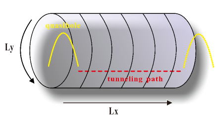
To study the quasiparticle tunneling of the Laughlin state at , a quasihole with charge or is put on one edge of the cylinder as shown in Fig.1. Here the model wavefunction for Laughlin state can be obtained by diagonalizing the model Hamiltonian with hard-core interaction, or just in the language of the Haldane’s pesudopotential. It can also be obtained by using the Jacks with the so called root configuration “”. The quasihole state for and is just the translated states with one and two sites along direction respectively. Or we can say a quasihole is inserted at the left edge of the finite cylinder which is represented as roots “” and “” for and respectively in the Jack polynomial description. A simple single particle tunneling potential
is assumed. It describes a tunneling path along the direction and therefore breaks the translational symmetry in direction. Then the matrix element is , which is related to the tunneling of an electron from the single particle state to state , is (set )
| (2) |
It is clearly that where is the distance between the two Gaussians. The many-body tunneling operator can be written as the summation of ones for single particle . Then we can calculate the tunneling amplitude for many-body wave function in which the and are the ground state and quasihole state wave function respectively. In this section, we just consider the tunneling amplitudes for and quasiholes in Laughlin state at . The matrix elements consist of contributions from the respective Slater-determinant components and . There are nonzero contributions only when the two sets and are identical except for a single pair and with angular momentum difference for and for where is the number of electrons. Therefore, we have and . The tunneling amplitude in the second quantization can be written as:
From the Eq. 2, it is known that the tunneling amplitude decreases exponentially as increasing the tunneling distance which is proportional to . The distance of the quasiparticle tunneling of mang-body state, or the length of the cylinder is determined by the size of the system and the aspect ratio . For a -particle system at fixed filling factor, the can be tuned from to by changing the aspect ratio . As that on the disk, a numerous of quasiholes were added at the center which makes the radius changes from to . And with a given , the distance between two single particle orbitals on cylinder is a constant which makes the tunneling distance scale proportional to the system size, i.e., on cylinder comparing with on disk. The linear relation guarantees a smooth change while varying .
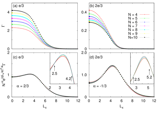
Fig. 2(a) and (b) show the tunneling amplitudes for and Laughlin quasihole as a function of the tunneling distance . When , or , the system is in a thin cylinder limit and the ground state is a crystal-like state in which electrons are separated, then the quasiparticle can not tunnel from one side to another, i.e., . On the other side, when , or , all the single particle orbitals collapse onto each other which corresponding to the ring limit on disk, or the CFT limit in which case the geometry factor of the many-body wave function can be neglected. Our previous studies [9, 10] show that the tunneling amplitude for and quasihole in the CFT limit for a system with electrons can be exactly represented as:
| (7) |
where and . For example, and . The numbers in the fractions are the position of the s in Eq. 2. Formally, the tunneling amplitude for quasihole for Laughlin state has an algebraic expression , in which for Laughlin state and the beta function is defined as . Fig. 2(a) and (b) show that the tunneling amplitudes saturates exactly at these CFT limit values when . In the medium region of , the tunneling amplitude has a dramatical change from these CFT values to zero. The state in this region is close to the Laughlin state, thus the signal of the decreasing of the quasihole tunneling amplitude can be seemed as a measurement of a phase transition (PT)-like from the thin cylinder state with zero tunneling amplitude to the CFT limit with a finite tunneling amplitude. Here we should note that we use the terminology PT-like instead of PT since there is actually no phase transition in the ground state while varying . The topological properties of the ground state in CFT limit are the same as that in the thin cylinder limit [21, 22, 23]. As shown in Fig. 2(c) and (d), the data for different system sizes collapse into each other after the following scaling conjecture is applied
| (8) |
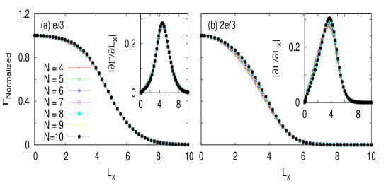
The exponent is related to the scaling dimension of the quasiparticle as . The Laughlin quasihole operator can be written as with a primary charge bosonic field in CFT. Therefore, the scaling dimension for and quasiholes are and respectively and then and . In disk geometry [8], the best scaling parameter for was which has a large deviation from the theoretical prediction. We think this deviation should come from the insufficient tunneling distance which is maximized at the radius of the disk. On the other hand, as we discussed above, the tunnel amplitude data near is missed due to the huge number of quasiholes needed to be insert at the center. On cylinder, as showed in Fig. 2(c) and (d), the scaling conjecture of Eq.8 works perfect when is large than a specific value. The reason we are saying this is that if we enlarge the rescaled data in the small region as shown in the inserted figure, crossover behaviors from different systems occur around and as shown by arrows in Fig. 2(c). The crossover at is also remained the same in Fig. 2(d) for quasihole. Here we should note that there is no crossover for larger in Fig. 2(d). However, we observe that the scaling behavior is starting to be broken down near . The first crossover at can be explained a transition from two dimensional system to one dimensional system. The 1D system corresponds to Calogero-Sutherland model [24] which actually is the origin of the holomorphic part of the FQH wave function, or the Jack polynomials [15, 16, 17]. The dimension reduction of the FQH state was also considered in the composite ferimion systems [25, 26]. Or we can say that the system is in the CFT limit while . The second critical value for and for is the transition point where the scaling behavior is broken down. This can be explained by the broken down of tunneling behavior between two independent edges due to gluing the two anti-propagating edges together when varying . Or we can say that the is the length scale at which two edges start to interact with each other. When , there are back scatterings between the two anti-propagating edges. The different values of between the and quasiholes should be from the size difference of them. Another way to extrapolate the critial point is renormalizing the data by its CFT value from Eq. 2 as shown in Fig. 3. Interestingly, the data for different sizes have a scaling-like behavior with collapsing onto one curve. The insert plots in Fig. 3 are the first order deviations of the normalized tunneling amplitudes. Again the first deviations have peaks at both for and by extrapolating to the thermodynamic limit with .
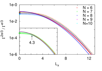
On the other hand, besides the dependence of the tunneling amplitudes, the Eq.8 tells us the ratio of the two types of tunneling amplitude is expected to has an asymptotic behavior which depends on :
| (9) |
In Fig.4, we plot the ratio as a function of for system with electrons. Unlike the data on disk [8] in which there was a sudden change while the first quasihole was inserted at the center, the ratio on the cylinder is smooth as a function of . The data in Fig.4 can be fitted by a solid line with which is consistent with the expected behavior in Eq.9. With comparison to the disk, the ratio of the tunneling amplitude for and for Moore-Read state on disk has an asymptotic which has a relative large deviation from the expected behavior . And for Laughlin state, the numerical and theoretical prediction are , respectively. Moreover, if we just plot the data for 10 electrons as insert plot in Fig.4, it is shown that the deviation of the asymptotic behavior occurs near which is close to . This deviation also demonstrates that the tunneling has been affected by the edge-edge interaction at this length scale.
3 Bipartite Entanglement entropy
The idea that the quantum entanglement [27] in a bipartite system can describe different phases of matter has emerged over the past years. This approach has provided plenty of new insights, while traditional methods based on symmetry breaking and local order parameters in Landau theory are fail. More precisely, a bipartition of the quantum system is defined when the Hilbert space factors into two parts . The bipartite FQH system can be implemented in both the momentum space and the real space of the two dimensional electron system. The former is called the orbital cut (OC) [28] and the later real space cut (RC) [29]. With a bipartition, a pure quantum state can be expressed in the form of Schmidt decomposition
| (10) |
where and are orthonormal sets in and respectively and the value of in Schmidt singular values are the entanglement “energies” in entanglement spectrum [30]. Equivalently, the reduced density matrix has eigenvalues . The Von Neumann entropy
| (11) |
generally scales linearly with the area of the cut between parts A and B and with a universal order correction, namely the topological entanglement entropy [31, 32, 33], i.e., . The topological entanglement entropy of the ground state for a fully gapped Hamiltonian is one robust measure of quantum entanglement in a topological phase in two dimension system. In the FQH state, where is the total quantum dimension of the system. For Laughlin state at , the quantum dimension is and therefore .
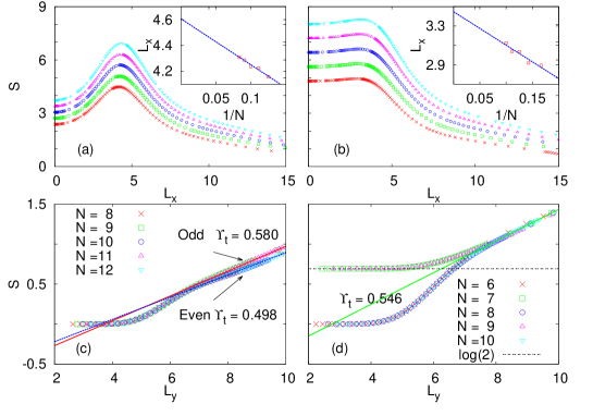
On the cylinder, we intend to divide the system into two equal subsystem with the same number of orbitals in OC or the same length in RC. However, the number of orbitals for -electron Laughlin state is which has the same parity as . Then the bipartition of the orbitals should has an even-odd effect, which can be defined as the orbital difference between and , namely is for even and, for odd . Intuitively, the effect of orbital difference should be diminished as increasing due to the local properties of the entanglement entropy, or inversely, it becomes more clear in small , or large region. This can be shown in Fig.5(c). In the RC case, it is easy to comprehend that even-odd effect exists, especially in the thin cylinder limit. Taking the and thin cylinder crystal-like states as examples, their wavefunction are single Slater-determinant and respectively. Then the position of the RC cut for state with even has zero electron density which induce a zero entanglement entropy. On the other hand, there is an electron locates at the position of the RC cut for odd electron TT state. Then the electron density reaches its maximum and the entanglement entropy saturates at a specific value, which is the same as that for cutting a single electron wave function into two equal parts which is the classical Von Neumann entropy which is shown in Fig.5(d). When the cylinder is bipartite along the direction, the is actually the length of the cutting, or the “area” between two subsystems. Then the topological entanglement entropy can be extrapolated from Fig.5(c) and (d). We found in the case of the OC, the data for systems have the same parity are sitting on the same curve as a function of . For large , they can linearly be fitted and the topological entanglement entropy for even and odd parities are and respectively. The exact value is in between them. A more accurate extrapolation can be obtained in RC entanglement entropy which shown in Fig.5(d) where the which is close to the exact value. An interesting phenomenon is both the OC and RC entanglement entropies saturate at zero ( for odd parity in RC) near . Therefore, we conclude that is the length scale in direction that the CDW behavior appears.
In Fig.5(a) and (b), we plot the bipartite entanglement with OC and RC as a function of . The OC entanglement entropy has a peak at in the thermodynamic limit as shown in the insert plot. In the RC, the peak of the entanglement entropy is not as sharp as that in the OC since the entropy while decreases very slowly. The position of the peak in the thermodynamic limit is . The error bar origins from the strong even-odd effect in this region. The difference between OC and RC can be explained by the different width of the cuts in realspace. The OC has a wider cut range and is more sensitive to the change of . It is known that the entanglement entropy has a singularity at the critical point of the QPT due to the divergence of the quantum fluctuation. However, since there is no phase transition occurs while varying the [21, 22, 23], the increment of the entanglement entropy origins from the correlations between two edges. Therefore, the two length scales and for OC and RC respectively should be related to the .
4 Electron Green’s Function
Tunneling characteristic at the edge has long been regarded as an experimental method of measuring the topological order of the FQH liquids. For tunneling from a three-dimensional Fermi liquid into the FQH edge, chiral Luttinger liquid theory [34] leads to a non-Ohmic tunneling relation with , in sharp contrast to the Ohmic prediction of a Fermi-liquid-dominated edge with . The electron Green’s function is defined as
| (12) |
where the and are field operators which create and annihilate an electron at position and respectively. If we consider the tunneling path along the edge of the FQH droplet, the edge Green’s function shows a scaling behavior with for long distance tunneling [35, 36].
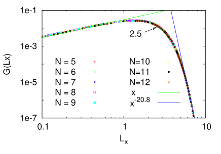
In this section, we consider the electron tunneling from the left edge of the cylinder to the right one, namely the electron correlation function between two anti-propagating edges as a function of . The results are shown in Fig.6. It shows that the Green’s function decreases dramatically when is larger than the saddle point which is the one dimensional limit threshold value . The data for large tunneling distance near obeys a power law behavior with an exponent less than . In the large limit, obviously, the Green’s function is zero in the Tao-Thouless state which is an insulator. We also checked the Laughlin state and found that the electron Green’s function has the same power law behavior in this region. Thus we think that the exponent in the large region depends on the interaction between electrons. The electron Green’s function scales as a which has a positive exponent one. Generally, the electron Green’s function at zero temperature decays as [37, 38] in which and is the “anomalous dimension” of the fermion operators. The case for corresponds to the normal Fermi liquid and is due to the correction of the electron-electron interaction which is the behavior of a Luttinger liquid. On the other hand, when , the system enters into a one dimensional phase which is described by the Calogero-Sutherland model. The reason that the correlation decreases as reducing is due to the repulsion between electrons, or strictly speaking, the electron Green’s function drop to zero in the 1D limit.
5 Summary and discussion
As a conclusion, we confirm that the quasihole tunneling amplitude in the cylinder geometry obeys the scaling conjecture in Eq.8 and the scaling behavior is much better than that on disk. Generally the scaling behavior works well when where for and for with a difference due to different size of the quasihole. The can be explained as the threshold value of the edge-edge back scattering between two edges. It appears not only in the quasihole tunneling amplitude calculations, but also in bipartite entanglement entropy. Therefore, the is the smallest length scale that guarantees there are two independent edges at two ends of the cylinder. It should be the benchmark of the sample size in designing of the experimental setup of the quasiparticle tunneling and interference [39, 40]. Moreover, we found another critical value , which is universal for different types of quasiholes. It can be explained as the critical width evolving from a 2D system to 1D system which is described by the Calogero-Sutherland model. Bipartite entanglement entropy has a singular behavior near due to a contribution of the edge-edge back scatterings. The topological entanglement entropy is extracted from the OC and RC entanglement entropies as a function of in a finite size system. The plays a role of a saddle point in the single particle Green’s function where the system enters into a one dimensional description. The scaling exponent of the Green’s function is one while approaching to the 1D limit. We notice that the is actually the correlation length of the Laughlin state as mentioned in the iDMRG calculation [41]. Here we should admit that we just consider the Laughlin state of the model Hamiltonian with hard-core interaction, or with pesudopotential. For a realistic coulomb interaction or the FQH state in higher Landau levels, we believe that the similar behaviors exists which may at most have small modifications on the value of these lengh scales.
We thank X. Wan and G. T. Liu for helpful discussions. This work was supported by NSFC Project No. 1127403 and Fundamental Research Funds for the Central Universities No. CQDXWL-2014-Z006. NJ is also supported by Chongqing Graduate Student Research Innovation Project No. CYB14033.
References
References
- [1] D. C. Tsui, H. L Stomer and A. C. Gossard, Phys. Rev. Lett. 48, 1559 (1982).
- [2] A. Kitaev, Ann. Phys. (N. Y.) 303, 2 (2003).
- [3] M. H. Freedom, Proc. Natl, Acad. Sci. U. S. A. 95, 98 (1998).
- [4] C. Nayak, S. H. Simon, A. Stern, M. Freedom and S. Das Sarma, Rev. Mod. Phys. 80, 1803 (2008).
- [5] C. de C. Chamon, D. E. Freed, S. A. Kivelson, S. L. Sondhi and X. G. Wen, Phys. Rev. B 55, 2331 (1997).
- [6] A. Stern and B. I. Halperin, Phys. Rev. Lett. 96, 016802 (2006).
- [7] P. Bonderson, A. Kitaev and K. Shtengel, Phys. Rev. Lett. 96, 016803 (2006).
- [8] H. Chen, Z-X. Hu, K. Yang, E.H. Rezayi and X. Wan, Phys. Rev. B 80, 235305 (2009).
- [9] Z-X. Hu, K-H. Lee, E. H. Rezayi, X. Wan and K. Yang, New J. Phys 13, 035020 (2011).
- [10] Z-X. Hu, K-H. Lee and X. Wan, Int. J. Mod. Phys. Conf. Ser. 11, 70 (2012).
- [11] R. Tao and D. J. Thouless, Phys. Rev. B 28, 1142 (1983).
- [12] D. J. Thouless, Surf. Sci. 142, 147 (1984).
- [13] E. H. Rezayi and F. D. M. Haldane, Phys. Rev. B 50, 17199 (1994).
- [14] B. Feigin, M. Jimbo, T. Miwa and E. Mukhin, Int. Math. Res. Not. 2002, 1223 (2002); ibid, 2003, 1015 (2003).
- [15] B. A. Bernevig and F. D. M. Haldane, Phys. Rev. Lett. 100, 246802 (2008).
- [16] B. A. Bernevig and F. D. M. Haldane, Phys. Rev. Lett. 101, 246806 (2008).
- [17] B. A. Bernevig and N. Regnault, Phys. Rev. Lett. 103, 206801 (2009).
- [18] K-H. Lee, Z-X. Hu and X. Wan, Phys. Rev. B 89, 165124 (2014).
- [19] B. Yang, Z-X. Hu, Z. Papić and F. D. M. Haldane, Phys. Rev. Lett. 108, 256807 (2012).
- [20] Z-X. Hu, Z. Papic, S. Johri, R.N. Bhatt and P. Schmitteckert, Phys. Lett. A 376, 2157 (2012).
- [21] A. Seidel, H. Fu, D-H. Lee, J. M. Leinaas, and J. Moore, Phys. Rev. Lett. 95, 266405 (2005).
- [22] E. J. Bergholtz and A. Karlhede, Phys. Rev. B 77, 155308 (2008).
- [23] E. J. Bergholtz, T. H. Hansson, M. Hermanns, A. Karlhede and S. Viefers, Phys. Rev. B 77, 165325 (2008).
- [24] F. Calogero, J. Math. Phys. 10, 2197 (1969); B. Sutherland, 12, 246 (1971); ibid.12, 251 (1971).
- [25] J. K. Jain, Phys. Rev. B 41, 7653 (1990).
- [26] Y. Yu, Phys. Rev. B 61, 4465 (2000).
- [27] M. A. Nielsen and I. L. Chuang, Quantum Computation and Quantum Information(Cambridge, 2000).
- [28] M. Haque, O. Zozulya and K. Schoutens, Phys. Rev. Lett. 98, 060401 (2007); O.S. Zozulya et al., Phys. Rev. B 76, 125310 (2007).
- [29] J. Dubail, N. Read and E. H. Rezayi, Phys. Rev. B 85, 115321 (2012) ; A. Sterdyniak, A. Chandran, N. Regnault, B. A. Bernevig and P. Bonderson, Phys. Rev. B 85, 125308 (2012).
- [30] H. Li and F. D. M. Haldane, Phys. Rev. Lett. 101, 010504 (2008).
- [31] A. Hamma, R. Ionicioiu and P. Zanardi, Phys. Lett. A 337, 22 (2005).
- [32] A. Kitaev and J. Preskill, Phys. Rev. Lett. 96, 110404 (2006).
- [33] M. Levin and X. G. Wen, Phys. Rev. Lett. 96, 110405 (2006).
- [34] X. G. Wen, Int. J. Mod. Phys. B 6, 1711 (1992).
- [35] X. Wan, F. Evers and E. H. Rezayi, Phys. Rev. Lett. 94, 166804 (2005).
- [36] Z-X. Hu, R. N. Bhatt, X. Wan and K. Yang, J. Phys.: Conf. Ser. 402, 012017 (2012).
- [37] A. Luther and I. Peschel, Phys. Rev. B 9, 2911 (1974).
- [38] A. Theumann, J. Math. Phys. 8, 2460 (1967).
- [39] R. L. Willett, L. N. Pfeiffer and K. W. West, Proc. Natl. Acad. Sci. U.S.A. 106, 8853 (2009).
- [40] R. L. Willett, L. N. Pfeiffer, and K. W. West, Phys. Rev. B 82, 205301 (2010).
- [41] M. P. Zaletel, R. S. K. Mong, F. Pollman, and E. H. Rezayi, Phys. Rev. B 91 045115 (2015).