Abstract

An important form of prior information in clustering comes in form of cannot-link and must-link constraints. We present a generalization of the popular spectral clustering technique which integrates such constraints. Motivated by the recently proposed $1$-spectral clustering for the unconstrained problem, our method is based on a tight relaxation of the constrained normalized cut into a continuous optimization problem. Opposite to all other methods which have been suggested for constrained spectral clustering, we can always guarantee to satisfy all constraints. Moreover, our soft formulation allows to optimize a trade-off between normalized cut and the number of violated constraints. An efficient implementation is provided which scales to large datasets. We outperform consistently all other proposed methods in the experiments.

1 Introduction

The task of clustering is to find a natural grouping of items given e.g. pairwise similarities. In real world problems, such a natural grouping is often hard to discover with given similarities alone or there is more than one way to group the given items. In either case, clustering methods benefit from domain knowledge that gives bias to the desired clustering. Wagstaff et. al [17] are the first to consider constrained clustering by encoding available domain knowledge in the form of pairwise must-link (ML, for short) and cannot-link (CL) constraints. By incorporating these constraints into $k$-means they achieve much better performance. Since acquiring such constraint information is relatively easy, constrained clustering has become an active area of research; see [1] for an overview.

Spectral clustering is a graph-based clustering algorithm originally derived as a relaxation of the NP-hard normalized cut problem. The spectral relaxation leads to an eigenproblem for the graph Laplacian, see [7, 14, 16]. However, it is known that the spectral relaxation can be quite loose [6]. More recently, it has been shown that one can equivalently rewrite the discrete (combinatorial) normalized Cheeger cut problem into a continuous optimization problem using the nonlinear $1$-graph Laplacian [8, 15] which yields much better cuts than the spectral relaxation. In further work it is shown that even all balanced graph cut problems, including normalized cut, have a tight relaxation into a continuous optimization problem [9].

The first approach to integrate constraints into spectral clustering was based on the idea of modifying the weight matrix in order to enforce the must-link and cannot-link constraints and then solving the resulting unconstrained problem [11]. Another idea is to adapt the embedding obtained from the first $k$ eigenvectors of the graph Laplacian [12]. Closer to the original normalized graph cut problem are the approaches that start with the optimization problem of the spectral relaxation and add constraints that encode must-links and cannot-links [20, 5, 19, 18]. Furthermore, the case where the constraints are allowed to be inconsistent is considered in [4].

In this paper we contribute in various ways to the area of graph-based constrained learning. First, we show in the spirit of $1$-spectral clustering [8, 9], that the constrained normalized cut problem has a tight relaxation as an unconstrained continuous optimization problem. Our method, which we call COSC, is the first one in the field of constrained spectral clustering, which can guarantee that all given constraints are fulfilled. While we present arguments that in practice it is the best choice to satisfy all constraints even if the data is noisy, in the case of inconsistent or unreliable constraints one should refrain from doing so. Thus our second contribution is to show that our framework can be extended to handle degree-of-belief and even inconsistent constraints. In this case COSC optimizes a trade-off between having small normalized cut and a small number of violated constraints. We present an efficient implementation of COSC based on an optimization technique proposed in [9] which scales to large datasets. While the continuous optimization problem is non-convex and thus convergence to the global optimum is not guaranteed, we can show that our method improves any given partition which satisfies all constraints or it stops after one iteration.

All omitted proofs and additional experimental results can be found in the supplementary material.

Notation. Set functions are denoted by a hat, $\hat{S}$, while the corresponding extension is $S$. In this paper, we consider the normalized cut problem with general vertex weights. Formally, let $G(V,E,w,b)$ be an undirected graph $G$ with vertex set $V$ and edge set $E$ together with edge weights $w:V\times V\rightarrow\mathbb{R}_{+}$ and vertex weights $b:V\rightarrow\mathbb{R}_{+}$ and $n=|V|$. Let $C\subset V$ and denote by $\overline{C}=V\backslash C$. We define respectively the cut, the generalized volume and the normalized cut (with general vertex weights) of a partition $(C,\overline{C})$ as

$$\mathrm{cut}(C,\overline{C})=2\sum_{i\in C,\,j\in\overline{C}}w_{ij}, \mathrm{gvol}(C)=\sum_{i\in C}b_{i},$$

$$\mathrm{bal}(C)=2\frac{\mathrm{gvol}(C)\mathrm{gvol}(\overline{C})}{\mathrm{gvol}(V)}, \mathrm{NCut}(C,\overline{C})=\frac{\mathrm{cut}(C,\overline{C})}{\mathrm{bal}(C)}.$$

We obtain ratio cut and normalized cut for special cases of the vertex weights, $b_{i}=1,\ \textrm{and}\ b_{i}=d_{i},\textrm{where}\ d_{i}=\sum_{j=1}^{n}w_{ij}$, respectively. In the ratio cut case, $\mathrm{gvol}(C)$ is the cardinality of $C$ and in the normalized cut case, it is volume of $C$, denoted by $\mathop{\rm vol}\nolimits(C)$.

2 The Constrained Normalized Cut Problem

We consider the normalized cut problem with must-link and cannot-link constraints. Let $G(V,E,w,b)$ denote the given graph and $Q^{m}$, $Q^{c}$ be the constraint matrices, where the element $q^{m}_{ij}$ (or $q^{c}_{ij}$) $\in\{0,1\}$ specifies the must-link (or cannot-link) constraint between $i$ and $j$. We will in the following always assume that $G$ is connected. All what is stated below and our suggested algorithm can be easily generalized to degree of belief constraints by allowing $q^{m}_{ij}$ (and $q^{c}_{ij}$) $\in[0,1]$. However, in the following we consider only $q_{ij}$ (and $q^{c}_{ij}$) $\in\{0,1\}$, in order to keep the theoretical statements more accessible.

Definition 2.1.

We call a partition $(C,\overline{C})$ consistent if it satisfies all constraints in $Q^{m}$ and $Q^{c}$.

Then the constrained normalized cut problem is to minimize $\mathrm{NCut}(C,\overline{C})$ over all consistent partitions. If the constraints are unreliable or inconsistent one can relax this problem and optimize a trade-off between normalized cut and the number of violated constraints. In this paper, we address both problems in a common framework.

We define the set functions, $M,N:2^{V}\rightarrow\mathbb{R}$, as

$$\hat{M}(C) :=2\sum_{i\in C,\,j\in\overline{C}}q^{m}_{ij}$$

$$\hat{N}(C) :=\sum_{i\in C,\,j\in C}q^{c}_{ij}+\sum_{i\in\overline{C},\,j\in\overline{C}}q^{c}_{ij}=\mathop{\rm vol}\nolimits(Q^{c})-2\sum_{i\in C,\,j\in\overline{C}}q^{c}_{ij}.$$

$\hat{M}(C)$ and $\hat{N}(C)$ are equal to twice the number of violated must-link and cannot-link constraints of partition $(C,\overline{C})$.

As we show in the following, both the constrained normalized cut problem and its soft version can be addressed by minimization of $\hat{F}_{\gamma}:2^{V}\rightarrow\mathbb{R}$ defined as

$$\hat{F}_{\gamma}(C)=\frac{\mathrm{cut}(C,\overline{C})+\gamma\,\big{(}\hat{M}(C)+\hat{N}(C)\big{)}}{\mathrm{bal}(C)},$$ (1)

where $\gamma\in\mathbb{R}_{+}$. Note that $\hat{F}_{\gamma}(C)=\mathrm{NCut}(C,\overline{C})$ if $(C,\overline{C})$ is consistent. Thus the minimization of $\hat{F}_{\gamma}(C)$ corresponds to a trade-off between having small normalized cut and satisfying all constraints parameterized by $\gamma$.

The relation between the parameter $\gamma$ and the number of violated constraints by the partition minimizing $\hat{F}_{\gamma}$ is quantified in the following lemma.

Lemma 2.1.

Let $(C,\overline{C})$ be consistent and $\lambda=\mathrm{NCut}(C,\overline{C})$. If $\gamma\geq\frac{\mathrm{gvol}(V)}{4(l+1)}\lambda$, then any minimizer of $\hat{F_{\gamma}}$ violates no more than $l$ constraints.

Proof.

Any partition $(C,\overline{C})$ that violates more than $l$ constraints satisfies $\hat{M}(C)+\hat{N}(C)\geq 2(l+1)$ and thus

$$\hat{F}_{\gamma}(C) =\mathrm{NCut}(C,\overline{C})+\gamma\ \frac{\hat{M}(C)+\hat{N}(C)}{\mathrm{bal}(C)}$$

$$\geq\mathrm{NCut}(C,\overline{C})+\frac{\gamma 2(l+1)}{\frac{1}{2}\mathrm{gvol}(V)}>\frac{4\gamma(l+1)}{\mathrm{gvol}(V)},$$

where we have used that $\max_{C}\mathrm{bal}(C)=\mathrm{gvol}(V)/2$ and $\mathrm{NCut}(C,\overline{C})>0$ as the graph is connected. Assume now that the partition $(D,\overline{D})$ minimizes $\hat{F}_{\gamma}$ for $\gamma=\frac{\mathrm{gvol}(V)}{4(l+1)}\lambda$ and violates more than $l$ constraints. Then

$$\hat{F}_{\gamma}(D) >\frac{4\gamma(l+1)}{\mathrm{gvol}(V)}\geq\lambda=\hat{F_{\gamma}}(C),$$

which leads to a contradiction. ∎

Note that it is easy to construct a partition which is consistent and thus the above choice of $\gamma$ is constructive. The following theorem is immediate from the above lemma for the special case $l=0$.

Theorem 2.1.

Let $(C,\overline{C})$ be consistent with the given constraints and $\lambda=\mathrm{NCut}(C,\overline{C})$. Then for $\gamma\geq\frac{\mathrm{gvol}(V)}{4}\ \lambda$, it holds that

$$\mathop{\rm arg\,min}\limits_{\begin{subarray}{c}C\subset V:\\ (C,\overline{C})\ \textrm{consistent}\end{subarray}}\mathrm{NCut}(C,\overline{C})=\mathop{\rm arg\,min}\limits_{C\subset V}\hat{F}_{\gamma}(C)$$

and the optimum values of both problems are equal.

Thus the constrained normalized cut problem can be equivalently formulated as the combinatorial problem of minimizing $\hat{F}_{\gamma}$. In the next section we will show that this problem allows for a tight relaxation into a continuous optimization problem.

2.1 A tight continuous relaxation of $\hat{F}_{\gamma}$

Minimizing $\hat{F}_{\gamma}$ is a hard combinatorial problem. In the following, we derive an equivalent continuous optimization problem. Let $f:\mathbb{R}^{V}\rightarrow\mathbb{R}$ denote a function on $V$, and $\mathbf{1}_{C}$ denote the vector that is 1 on $C$ and 0 elsewhere. Define

$$M(f) :=\sum_{i,j=1}^{n}q^{m}_{ij}\left|f_{i}-f_{j}\right|\textrm{and}$$

$$N(f) :=\mathop{\rm vol}\nolimits(Q^{c})\big{(}\max(f)-\min(f)\big{)}-\sum_{i,j=1}^{n}q^{c}_{ij}\left|f_{i}-f_{j}\right|,$$

where $\max(f)$ and $\min(f)$ are respectively the maximum and minimum elements of $f$. Note that $M(\mathbf{1}_{C})=\hat{M}(C)$ and $N(\mathbf{1}_{C})=\hat{N}(C)$ for any non-trivial partition $(C,\overline{C})$.

Let $B$ denote the diagonal matrix with the vertex weights $b$ on the diagonal. We define

$$F_{\gamma}(f)=\frac{\sum_{i,j=1}^{n}w_{ij}\left|f_{i}-f_{j}\right|+\gamma\ M(f)+\gamma\ N(f)}{{\left\|B(f-\frac{1}{\mathrm{gvol}(V)}\left\langle f,b\right\rangle\mathbf{1})\right\|_{1}}}.$$

We denote the numerator of $F_{\gamma}(f)$ by $R_{\gamma}(f)$ and the denominator by $S(f)$.

Lemma 2.2.

For any non-trivial partition it holds that $\hat{F}_{\gamma}(C)=F_{\gamma}(\mathbf{1}_{C})$.

Proof.

We have,

$$\sum_{i,j=1}^{n}w_{ij}|(\mathbf{1}_{C})_{i}-(\mathbf{1}_{C})_{j}|=\mathrm{cut}(C,\overline{C})$$

$$\left\|B(\mathbf{1}_{C}-\frac{1}{\mathrm{gvol}(V)}\left\langle\mathbf{1}_{C},b\right\rangle\mathbf{1})\right\|_{1}$$

$$= \left\|B\Big{(}\big{(}1-\frac{\mathrm{gvol}(C)}{\mathrm{gvol}(V)}\big{)}\mathbf{1}_{C}-\frac{\mathrm{gvol}(C)}{\mathrm{gvol}(V)}\mathbf{1}_{\overline{C}}\Big{)}\right\|_{1}$$

$$= \big{(}1-\frac{\mathrm{gvol}(C)}{\mathrm{gvol}(V)}\big{)}\mathrm{gvol}(C)+\frac{\mathrm{gvol}(C)}{\mathrm{gvol}(V)}\mathrm{gvol}(\overline{C})=\mathrm{bal}(C)$$

This together with the discussion on $M,N$ finishes the proof. ∎

From Lemma 2.2 it immediately follows that minimizing $F_{\gamma}$ is a relaxation of minimizing $\hat{F}_{\gamma}$. In our main result (Theorem 2.2), we establish that both problems are actually equivalent, so that we have a tight relaxation. In particular a minimizer of $F_{\gamma}$ is an indicator function corresponding to the optimal partition minimizing $\hat{F}_{\gamma}$.

The proof is based on the following key property of the functional $F_{\gamma}$. Given any non-constant $f\in\mathbb{R}^{n}$, optimal thresholding,

$$C^{*}_{f}=\mathop{\rm arg\,min}\limits_{\min_{i}f_{i}\ \leq\ t\ <\ \max_{i}f_{i}}\hat{F}_{\gamma}(C^{t}_{f}),$$

where $C^{t}_{f}=\{i\in V|f_{i}>t\}$, yields an indicator function on some $C^{*}_{f}\subset V$ with smaller or equal value of $F_{\gamma}$.

Theorem 2.2.

For $\gamma\geq 0$, we have

$$\min_{C\subset V}\hat{F}_{\gamma}(C)\ =\ \min_{f\in\mathbb{R}^{n},\ f\textrm{ non-constant}}F_{\gamma}(f).$$

Moreover, a solution of the first problem can be obtained from the solution of the second problem.

Proof.

It has been shown in [8], that

$$\sum_{i,j=1}^{n}w_{ij}|f_{i}-f_{j}| =\ \int_{-\infty}^{\infty}\mathrm{cut}(C^{t}_{f},\overline{C^{t}_{f}})dt$$

We define $\hat{P}:2^{V}\rightarrow\mathbb{R}$ as $\hat{P}(C)=1$, if $C\neq V$ and $C\neq\emptyset$, and $0$ otherwise. Denoting by $\mathrm{cut}_{Q}(C,\overline{C})$, the cut on the constraint graph whose weight matrix is given by $Q$, we have

$$R_{\gamma}(f) =\ \int_{-\infty}^{\infty}\mathrm{cut}(C^{t}_{f},\overline{C^{t}_{f}})dt+\gamma\ \int_{-\infty}^{\infty}\mathrm{cut}_{Q^{m}}(C^{t}_{f},\overline{C^{t}_{f}})$$

$$+\gamma\mathop{\rm vol}\nolimits(Q^{c})\int_{\min_{i}f_{i}}^{\max_{i}f_{i}}1dt-\gamma\ \int_{-\infty}^{\infty}\mathrm{cut}_{Q^{c}}(C^{t}_{f},\overline{C^{t}_{f}})$$

$$=\ \int_{-\infty}^{\infty}\mathrm{cut}(C^{t}_{f},\overline{C^{t}_{f}})dt+\gamma\ \int_{-\infty}^{\infty}\mathrm{cut}_{Q^{m}}(C^{t}_{f},\overline{C^{t}_{f}})$$

$$+\gamma\mathop{\rm vol}\nolimits(Q^{c})\int_{-\infty}^{\infty}\hat{P}(C^{t}_{f})dt-\gamma\ \int_{-\infty}^{\infty}\mathrm{cut}_{Q}^{c}(C^{t}_{f},\overline{C^{t}_{f}})$$

$$=\int_{-\infty}^{\infty}\hat{R}_{\gamma}(C^{t}_{f})\,dt$$

Note that $S(f)$ is an even, convex and positively one-homogeneous function. Moreover, every even, convex positively one-homogeneous function, $T:\mathbb{R}^{V}\rightarrow\mathbb{R}$ has the form $T(f)=\sup_{u\in U}\left\langle u,f\right\rangle$, where $U$ is a symmetric convex set, see e.g., [10]. Note that $S(\mathbf{1})=0$ and thus because of the symmetry of $U$ it has to hold $\left\langle u,\mathbf{1}\right\rangle=0$ for all $u\in U$. Since $S(\mathbf{1}_{C^{t}_{f}})=\hat{S}(C^{t}_{f})$ and $\ \left\langle u,f\right\rangle\leq S(f),u\in U$, we have for all $u\in U$,

$$R_{\gamma}(f) \geq\int_{-\infty}^{\infty}\frac{\hat{R}_{\gamma}(C^{t}_{f})}{\hat{S}(C^{t}_{f})}\ \left\langle u,\mathbf{1}_{C^{t}_{f}}\right\rangle dt$$

$$\geq\inf_{t\in\mathbb{R}}\frac{\hat{R}_{\gamma}(C^{t}_{f})}{\hat{S}(C^{t}_{f})}\int_{\min_{i}f_{i}}^{\max_{i}f_{i}}\ \left\langle u,\mathbf{1}_{C^{t}_{f}}\right\rangle dt,$$ (2)

where in the last inequality we changed the limits of integration using the fact that $\left\langle u,\mathbf{1}\right\rangle=0$. Let $C_{i}:=C^{t}_{f_{i}}$ and $C_{0}=V$. Then

$$\int_{\min_{i}f_{i}}^{\max_{i}f_{i}}\left\langle u,\mathbf{1}_{C_{i}}\right\rangle dt=\sum_{i=1}^{n-1}\left\langle u,\mathbf{1}_{C_{i}}\right\rangle(f_{i+1}-f_{i})=$$

$$\sum_{i=1}^{n}f_{i}\big{(}\left\langle u,\mathbf{1}_{C_{i-1}}\right\rangle-\left\langle u,\mathbf{1}_{C_{i}}\right\rangle\big{)}=\sum_{i=1}^{n}f_{i}u_{i}=\ \left\langle u,f\right\rangle$$

Noting that (2.1) holds for all $u\in U$, we have

$$R_{\gamma}(f)\geq\inf_{t\in\mathbb{R}}\hat{F}_{\gamma}(C^{t}_{f})\ \sup_{u\in U}\ \left\langle u,f\right\rangle=\inf_{t\in\mathbb{R}}\hat{F}_{\gamma}(C^{t}_{f})\ S(f).$$

This implies that

$$F_{\gamma}(f)\geq\inf_{t\in\mathbb{R}}\hat{F}_{\gamma}(C^{t}_{f})=F_{\gamma}(\mathbf{1}_{C^{*}_{f}}),$$ (3)

where $C^{*}_{f}=\mathop{\rm arg\,min}\limits_{\min_{i}f_{i}\ \leq\ t\ <\ \max_{i}f_{i}}\hat{F}_{\gamma}(C^{t}_{f})$.

This shows that we always get descent by optimal thresholding. Thus the actual minimizer of $F_{\gamma}$ is a two-valued function, which can be transformed to an indicator function on some $C\subset V$, because of the scale and shift invariance of $F_{\gamma}$. Then from Lemma 2.2, which shows that for non-trivial partitions, $\hat{F}_{\gamma}(C)=F_{\gamma}(\mathbf{1}_{C})$, the statement follows. ∎

Now, we state our second result: the problem of minimizing the functional $F_{\gamma}$ over arbitrary real-valued non-constant $f$, for a particular choice of $\gamma$, is in fact equivalent to the NP-hard problem of minimizing normalized cut with constraints.

Theorem 2.3.

Let $(C,\overline{C})$ be consistent and $\lambda=\mathrm{NCut}(C^{\prime},\overline{C^{\prime}})$. Then for $\gamma\geq\frac{\mathrm{gvol}(V)}{4}\ \lambda$, it holds that

$$\min_{\begin{subarray}{c}C\subset V:\\ (C,\overline{C})\ \textrm{consistent}\end{subarray}}\mathrm{NCut}(C,\overline{C})=\min_{f\in\mathbb{R}^{n},\ f\textrm{ non-constant}}F_{\gamma}(f)$$

Furthermore, an optimal partition of the constrained problem can be obtained from a minimizer of the right problem.

Proof.

From Theorem 2.1 we know that, for the chosen value of $\gamma$, the constrained problem is equivalent to

$$\min_{C\subset V}\hat{F}_{\gamma}(C),$$

which in turn is equivalent, by Theorem 2.2, to the right problem in the statement. Moreover, as shown in Theorem 2.2, minimizer of $F_{\gamma}$ is an indicator function on $C\subset V$ and hence we immediately get an optimal partition of the constrained problem. ∎

A few comments on the implications of Theorem 2.3. First, it shows that the constrained normalized cut problem can be equivalently solved by minimizing $F_{\gamma}(f)$ for the given value of $\gamma$. The value of $\gamma$ depends on the normalized cut value of a partition consistent with given constraints. Note that such a partition can be obtained in polynomial time by 2-coloring the constraint graph as long as the constraints are consistent.

2.2 Integration of must-link constraints via sparsification

If the must-link constraints are reliable and therefore should be enforced, one can directly integrate them by merging the corresponding vertices together with re-definition of edge and vertex weights. In this way ones derives a new reduced graph, where the value of the normalized cut of all partitions that satisfy the must-link constraints are preserved.

The construction of a reduced graph is given below for a must-link constraint $(p,q)$.

1. merge $p$ and $q$ into a single vertex $\tau$.

2. update the vertex weight of $\tau$ by $b_{\tau}=b_{p}+b_{q}$.

3. update the edges as follows: if $r$ is any vertex other than $p$ and $q$, then add an edge between $\tau$ and $r$ with weight $w(p,r)+w(q,r)$.

Note that this construction leads to a graph with vertex weights even if the original graph had vertex weights equal to $1$. If there are many must-links, one can efficiently integrate all of them together by first constructing the must-link constraint graph and merging each connected component in this way.

The following lemma shows that the above construction preserves all normalized cuts which respect the must-link constraints. We prove it for the simple case where we merge $p$ and $q$ and the proof can easily be extended to the general case by induction.

Lemma 2.3.

Let $G^{\prime}(V^{\prime},E^{\prime},w^{\prime},b^{\prime})$ be the reduced graph of $G(V,E,w,b)$ obtained by merging vertices $p$ and $q$. If a partition $(C,\overline{C})$ does not separate $p$ and $q$, we have $\mathrm{NCut}_{G}(C,\overline{C})=\mathrm{NCut}_{G^{\prime}}(C^{\prime},\overline{C^{\prime}})$.

Proof.

Note that $\mathrm{gvol}(V^{\prime})=\mathrm{gvol}(\tau)+\mathrm{gvol}(V\backslash\{p,q\})=\mathrm{gvol}(p)+\mathrm{gvol}(q)+\mathrm{gvol}(V\backslash\{p,q\})=\mathrm{gvol}(V)$. If $(C,\overline{C})$ does not separate $p$ and $q$, then we have either $\tau\subset C$ or $\tau\subset\overline{C}$. W.l.o.g. assume that $\tau\subset C$. The corresponding partition of $V^{\prime}$ is then $C^{\prime}=\tau\cup(C\ \{p,q\})$ and $\overline{C^{\prime}}=\overline{C}$. We get

$$\mathrm{cut}(C^{\prime},\overline{C^{\prime}}) =\sum_{i\in C^{\prime},j\in\overline{C^{\prime}}}w^{\prime}_{ij}=\sum_{j\in\overline{C^{\prime}}}w^{\prime}_{\tau j}+\sum_{i\in C^{\prime}\backslash\tau,j\in\overline{C^{\prime}}}w^{\prime}_{ij}$$

$$=\sum_{k\in\{p,q\},j\in\overline{C}}w_{kj}+\sum_{i\in C\backslash\{p,q\},j\in\overline{C}}w_{ij}=\mathrm{cut}(C,\overline{C}).$$

$$\mathrm{gvol}(C^{\prime}) =\sum_{i\in C^{\prime}}b^{\prime}_{i}=b^{\prime}_{\tau}+\sum_{i\in C^{\prime}\backslash\tau}$$

$$=b_{p}+b_{q}+\sum_{i\in C\backslash\{p,q\}}b_{i}=\sum_{i\in C}b_{i}=\mathrm{gvol}(C).$$

$$\mathrm{gvol}(\overline{C^{\prime}}) =\sum_{i\in\overline{C^{\prime}}}b^{\prime}_{i}=\sum_{i\in\overline{C}}b_{i}=\mathrm{gvol}(\overline{C}).$$

Thus we have $\mathrm{NCut}_{G}(C,\overline{C})=\mathrm{NCut}_{G^{\prime}}(C^{\prime},\overline{C^{\prime}})$ ∎

All partitions of the reduced graph fulfill all must-link constraints and thus any relaxation of the unconstrained normalized cut problem can now be used. Moreover, this is not restricted to the cut criterion we are using but any other graph cut criterion based on cut and the volume of the subsets will be preserved in the reduction.

3 Algorithm for Constrained $1$-Spectral Clustering

In this section we discuss the efficient minimization of $F_{\gamma}$ based on recent ideas from unconstrained $1$-spectral clustering [8, 9]. Note, that $F_{\gamma}$ is a non-negative ratio of a difference of convex (d.c) function and a convex function, both of which are positively one-homogeneous. In recent work [8, 9], a general scheme, shown in Algorithm 1 (where $\partial S(f)$ denotes the subdifferential of the convex function $S$ at $f$), is proposed for the minimization of a non-negative ratio of a d.c function and convex function both of which are positively one-homogeneous.

It is shown in [9] that Algorithm 1 generates a sequence $f^{k}$ such that either $F_{\gamma}(f^{k+1})<F_{\gamma}(f^{k})$ or the sequence terminates. Moreover, the cluster points of $f^{k}$ correspond to critical points of $F_{\gamma}$. The scheme is given in Algorithm 1 for the problem $\min_{f\in\mathbb{R}^{n}}(R_{1}(f)-R_{2}(f))/S(f)$, where

$$R_{1}(f) :=\frac{1}{2}\sum_{i,j=1}^{n}(w_{ij}+\gamma q^{m}_{ij})|f_{i}-f_{j}|$$

$$+\frac{\gamma}{2}\sum_{i,j=1}^{n}q^{c}_{ij}(\max(f)-\min(f))$$

$$R_{2}(f) :=\frac{1}{2}\sum_{i,j=1}^{n}q^{c}_{ij}|f_{i}-f_{j}|,\qquad$$

$$S(f) :=\frac{1}{2}\left\|B(f-\frac{1}{\mathrm{gvol}(V)}\left\langle f,b\right\rangle\mathbf{1})\right\|_{1}$$

Note that $R_{1},\,R_{2}$ are both convex functions and $F_{\gamma}(f)=(R_{1}(f)-R_{2}(f))/S(f)$.

Algorithm 1 Minimization of a ratio $(R_{1}(f)-R_{2}(f))/S(f)$ where $R_{1},R_{2},S$ are convex and positively one-homogeneous

1:  Initialization: $f^{0}=\text{random}$ with $\left\|f^{0}\right\|=1$, $\lambda^{0}=(R_{1}(f^{0})-R_{2}(f^{0}))/S(f^{0})$

2:  repeat

3:     $f^{k+1}=\mathop{\rm arg\,min}\limits_{\left\|f\right\|_{2}\leq 1}\left\{R_{1}(f)-\left\langle f,r_{2}\right\rangle-\lambda^{k}\left\langle f,s\right\rangle\right\}$ where  $r_{2}\in\partial R_{2}(f^{k})$, $s\in\partial S(f^{k})$

4:     $\lambda^{k+1}=(R_{1}(f^{k+1})-R_{2}(f^{k+1})/S(f^{k+1})$

5:  until $\frac{\left|\lambda^{k+1}-\lambda^{k}\right|}{\lambda^{k}}<\epsilon$

6:  Output: $\lambda^{k+1}$ and $f^{k+1}$.

Moreover, it is shown in [9], that if one wants to minimize $(R_{1}(f)-R_{2}(f))/S(f)$ only over non-constant functions, one has to ensure that $\left\langle r_{2},\mathbf{1}\right\rangle=\left\langle s,\mathbf{1}\right\rangle=0$. Note, that

$$\partial S(f) =\frac{1}{2}(\mathbb{I}-\frac{1}{\mathrm{gvol}(V)}b\mathbf{1}^{T})B\mathop{\rm sign}\limits\big{(}f-\frac{\ \left\langle b,f\right\rangle}{\mathrm{gvol}(V)}\mathbf{1}\big{)}$$

$$\partial R_{2}(f) =\Big{\{}\sum_{j=1}^{n}q^{c}_{ij}u_{ij}\,|\,u_{ij}=-u_{ji},\,u_{ij}\in\mathrm{sign}(f_{i}-f_{j})\Big{\}},$$

where $\mathop{\rm sign}\limits(x)=[-1,1]$ if $x=0$, otherwise it just the sign function. It is easy to check that $\left\langle u,\mathbf{1}\right\rangle=0$ for all $u\in\partial S(f)$ and all $f\in\mathbb{R}^{n}$ and there exists always a vector $u\in\partial R_{2}(f)$ for all $f\in\mathbb{R}^{n}$ such that $\left\langle u,\mathbf{1}\right\rangle=0$.

In the algorithm the key part is the inner convex problem which one has to solve at each step. In our case it has the form,

$$\min_{\left\|f\right\|_{2}\leq 1} \;\frac{1}{2}\sum_{i,j=1}^{n}(w_{ij}+\gamma q^{m}_{ij})\left|f_{i}-f_{j}\right|$$ (4)

$$+\frac{\gamma}{2}\sum_{i,j=1}^{n}q^{c}_{ij}(\max(f)-\min(f))-\left\langle f,\gamma\,r_{2}+\lambda^{k}s\right\rangle,$$

where $r_{2}\in\partial R_{2}(f^{k})$, $s\in\partial{S(f^{k})}$ and $\lambda^{k}=F_{\gamma}(f^{k})$.

To solve it more efficiently we derive an equivalent smooth dual formulation for this non-smooth convex problem. We replace $w_{ij}+\gamma q^{m}_{ij}$ by $w^{\prime}_{ij}$ in the following.

Lemma 3.1.

Let $E\subset V\times V$ denote the set of edges and $A:\mathbb{R}^{E}\rightarrow\mathbb{R}^{V}$ be defined as $(A\alpha)_{i}=\sum_{j|(i,j)\in E}w^{\prime}_{ij}\alpha_{ij}$. Moreover, let $U$ denote the simplex, $U=\{u\in\mathbb{R}^{n}\ |\ \sum_{i=1}^{n}u_{i}=1,u_{i}\geq 0,\ \forall i\}$. The above inner problem is equivalent to

$$\min_{\big{\{}\begin{subarray}{c}\alpha\in\mathbb{R}^{E}|\left\|\alpha\right\|_{\infty}\leq 1,\alpha_{ij}=-\alpha_{ji}\\ {v\in U}\end{subarray}\big{\}}}\Psi(\alpha,v):=$$ (5)

$$c\left\|-A\frac{\alpha}{c}+v+b-P_{U}\big{(}-A\frac{\alpha}{c}+v+b\big{)}\right\|_{2},$$

where $c=\frac{\gamma}{2}{\mathop{\rm vol}\nolimits(Q^{c})}$, $b=\frac{r_{2}}{c}+\lambda^{k}\frac{s}{c}$ and $P_{U}(x)$ is the projection of $x$ on to the simplex $U$.

Proof.

Noting that $\frac{1}{2}\sum_{i,j=1}^{n}w^{\prime}_{ij}\left|f_{i}-f_{j}\right|=\max_{\{\alpha\in\mathbb{R}^{E}|\left\|\alpha\right\|_{\infty}\leq 1,\alpha_{ij}=-\alpha_{ji}\}}\left\langle f,A\alpha\right\rangle$ (see [8]) and $\max_{i}f_{i}=\max_{u\in U}\left\langle u,f\right\rangle$, the inner problem can be rewritten as

$$\min_{\left\|f\right\|_{2}\leq 1}\max_{\{\alpha\in\mathbb{R}^{E}|\left\|\alpha\right\|_{\infty}\leq 1,\alpha_{ij}=-\alpha_{ji}\}}\left\langle f,A\alpha\right\rangle$$

$$+c\max_{u\in U}\left\langle f,u\right\rangle+c\max_{v\in U}\left\langle-f,v\right\rangle-\gamma\left\langle f,r_{2}\right\rangle-\lambda^{k}\left\langle f,s\right\rangle$$

$$=\min_{\left\|f\right\|_{2}\leq 1}\max_{\big{\{}\begin{subarray}{c}{\alpha\in\mathbb{R}^{E}|\left\|\alpha\right\|_{\infty}\leq 1,\alpha_{ij}=-\alpha_{ji}}\\ {u,v\in U}\end{subarray}\big{\}}}\left\langle f,A\alpha\right\rangle$$

$$+c\left\langle f,u\right\rangle-c\left\langle f,v\right\rangle-\gamma\left\langle f,r_{2}\right\rangle-\lambda^{k}\left\langle f,s\right\rangle$$

$${\stackrel{{\scriptstyle(s_{1})}}{{=}}}\max_{\begin{subarray}{c}{\alpha\in\mathbb{R}^{E}|}\\ {\left\|\alpha\right\|_{\infty}\leq 1}\\ {\alpha_{ij}=-\alpha_{ji}}\\ {u,v\in U}\end{subarray}}\min_{\left\|f\right\|_{2}\leq 1}\left\langle f,A\alpha+c(u-v)-\gamma r_{2}-\lambda^{k}s\right\rangle$$

$${\stackrel{{\scriptstyle(s_{2})}}{{=}}}\max_{\begin{subarray}{c}{\alpha\in\mathbb{R}^{E}|\left\|\alpha\right\|_{\infty}\leq 1}\\ {\alpha_{ij}=-\alpha_{ji}}{u,v\in U}\end{subarray}}-\left\|A\alpha-\gamma r_{2}-\lambda^{k}s+c(u-v)\right\|_{2}$$

$$=-\min_{\begin{subarray}{c}{\alpha\in\mathbb{R}^{E}|\left\|\alpha\right\|_{\infty}\leq 1}\\ {\alpha_{ij}=-\alpha_{ji}}\\ {u,v\in U}\end{subarray}}\Psi(\alpha,u,v).$$

The step $s_{1}$ follows from the standard min-max theorem (see Corollary 37.3.2 in [13]) since $u$, $v$, $\alpha$ and $f$ lie in non-empty compact convex sets. In the step $s_{2}$, we used that the minimizer of the linear function over the Euclidean ball is given by

$$f^{*}=\frac{A\alpha-\gamma r_{2}-\lambda^{k}s+cu-cv}{\left\|A\alpha-\gamma r_{2}-\lambda^{k}s+cu-cv\right\|_{2}},$$

if $\left\|A\alpha-\gamma r-\lambda^{k}s+cu-cv\right\|_{2}\neq 0$; otherwise $f^{*}$ is an arbitrary element of the Euclidean unit ball.

Finally, we have $\left\|A\alpha-r-\lambda^{k}s+cu-cv\right\|$ = c $\left\|A\frac{\alpha}{c}+u-v-b\right\|$. We also know that for a convex set $C$ and any given $y$, $\min_{x\in C}\left\|x-y\right\|=\left\|y-P_{C}(y)\right\|$, where $P_{C}(y)$ is the projection of $y$ onto the set $C$. With $y=-A\frac{\alpha}{c}+v+b$, we have for any $\alpha$, $\min_{u,v\in U}\Psi(\alpha,u,v)=\min_{v\in U}\min_{u\in U}c\left\|u-y\right\|=\min_{v\in U}c\left\|y-P_{U}(y)\right\|$ and from this the result follows. ∎

The smooth dual problem can be solved efficiently using first order projected gradient methods like FISTA [2], which has a guaranteed convergence rate of $O(\frac{L}{k^{2}})$, where $k$ is the number of steps, and $L$ is the Lipschitz constant of the gradient of the objective. The bound on the Lipschitz constant for the gradient of the objective in (5) can be rather loose if the weights are varying a lot. The rescaling of the variable $\alpha$ introduced in Lemma 3.2 leads to a better condition number and also to a tighter bound on the Lipschitz constant. This results in a significant improvement in practical performance.

Lemma 3.2.

Let $B$ be a linear operator defined as $(B\beta)_{i}:=\sum_{j:(i,j)\in E}\beta_{ij}$ and let $s_{ij}=\frac{w^{\prime}_{ij}}{c}{M}$, for positive constant $M\geq\left\|B\right\|$. The above inner problem is equivalent to

$$\min_{\begin{subarray}{c}\{\beta\in\mathbb{R}^{E}|\left\|\beta\right\|_{\infty}\leq s_{ij},\beta{ij}=-\beta_{ji}\}\\ {v\in U}\end{subarray}}\tilde{\Psi}(\beta,v):=\frac{1}{2}\left\|d-P_{U}(d)\right\|_{2}^{2},$$

where $d=-\frac{B}{M}\beta+v+b$. The Lipschitz constant of the gradient of $\tilde{\Psi}$ is upper bounded by 4.

Proof.

Let $\beta_{ij}=s_{ij}\alpha_{ij}$. Then $(A\frac{\alpha}{c})_{i}=\sum_{j:(i,j)\in E}w^{\prime}_{ij}\frac{\alpha_{ij}}{c}=\sum_{j:(i,j)\in E}\frac{\beta_{ij}}{M}=(\frac{B}{M}\beta)_{i}$ and constraints on $\alpha$ transform to $-s_{ij}\leq\beta_{ij}\leq s_{ij}$ and $\beta_{ij}=-\beta_{ij}$. Since the mapping between $\alpha$ and $\beta$ is one-to-one, the transformation yields an equivalent problem (in the sense that minimizer of one problem can be easily derived from minimizer of the other problem).

Now we derive a bound on the Lipschitz constant.

The gradient of $\Psi$ at $x=(\beta,v)$ w.r.t $\beta$, and $v$ are given by

$$(\nabla{\Psi(x)})_{\beta}=-\frac{B^{T}}{M}(d-P_{U}(d)),$$

$$(\nabla{\Psi(x)})_{v}=(d-P_{U}(d)),$$

where $B^{T}$ is the adjoint operator of $B$ given by $(B^{T}d)_{ij}=(d_{i}-d_{j})$.

Let $x^{\prime}=(\beta^{\prime},v^{\prime})$ denote any other point and $d^{\prime}=-\frac{B}{M}\beta^{\prime}+v^{\prime}+b$. then we have

$$\left\|\nabla{\Psi(x)}-\nabla{\Psi(x^{\prime})}\right\|^{2}$$

$$=\frac{\left\|B^{T}\right\|^{2}}{M^{2}}\left\|(d-P_{U}(d))-(d^{\prime}-P_{U}(d^{\prime})\right\|^{2}$$

$$+\left\|(d-P_{U}(d))-(d^{\prime}-P_{U}(d^{\prime}))\right\|^{2}$$

$$=\biggr{(}1+\frac{\left\|B^{T}\right\|^{2}}{M^{2}}\biggr{)}\left\|((d-d^{\prime})+(-P_{U}(d)+P_{U}(d^{\prime}))\right\|^{2}$$

$$\leq 2\ \biggr{(}1+\frac{\left\|B^{T}\right\|^{2}}{M^{2}}\biggr{)}(\left\|d-d^{\prime}\right\|^{2}+\left\|-P_{U}(d)+P_{U}(d^{\prime})\right\|^{2})$$

$$\leq 4\ \biggr{(}1+\frac{\left\|B^{T}\right\|^{2}}{M^{2}}\biggr{)}\left\|d-d^{\prime}\right\|^{2}$$

$$=4\ \biggr{(}1+\frac{\left\|B^{T}\right\|^{2}}{M^{2}}\biggr{)}\left\|\frac{B}{M}(-\beta+\beta^{\prime})+(v-v^{\prime})\right\|^{2}$$

$$\leq 4\biggr{(}1+\frac{\left\|B^{T}\right\|^{2}}{M^{2}}\biggr{)}\max\biggr{\{}\frac{\left\|B^{T}\right\|^{2}}{M^{2}},1\biggr{\}}$$

$$\ \left\|(-\beta+\beta^{\prime})+(v-v^{\prime})\right\|^{2}$$

$$\leq 8\ \biggr{(}1+\frac{\left\|B^{T}\right\|^{2}}{M^{2}}\biggr{)}\max\biggr{\{}\frac{\left\|B^{T}\right\|^{2}}{M^{2}},1\biggr{\}}$$

$$\ (\left\|\beta-\beta^{\prime}\right\|^{2}+\left\|v-v^{\prime})\right\|^{2})$$

$$=8\ \biggr{(}1+\frac{\left\|B^{T}\right\|^{2}}{M^{2}}\biggr{)}\max\biggr{\{}\frac{\left\|B^{T}\right\|^{2}}{M^{2}},1\biggr{\}}\ \left\|x-x^{\prime}\right\|^{2}$$

Hence the Lipschitz constant is upper bounded by $\sqrt{8\ \biggr{(}1+\frac{\left\|B^{T}\right\|^{2}}{M^{2}}\biggr{)}\max\biggr{\{}\frac{\left\|B^{T}\right\|^{2}}{M^{2}},1\biggr{\}}}\leq 4,$ since $M\geq\left\|B\right\|$. ∎

We can choose $M$ by upper bounding $\left\|B\right\|$ using

$$\left\|B\right\|^{2}\leq\max_{r}\sum_{(r,j)\in E}1^{2}=\max_{r}\mathrm{neigh}(r),$$

where $\mathrm{neigh}(r)$ is the number of neighbors of vertex $r$.

Despite the problem of minimizing $F_{\gamma}$ is non-convex and thus global convergence is not guaranteed, Algorithm 1 has the following quality guarantee.

Theorem 3.1.

Let $(C,\overline{C})$ be any partition and let $\lambda=\mathrm{NCut}(C,\overline{C})$. If one uses $\mathbf{1}_{C}$ as the initialization of the Algorithm 1, then the algorithm either terminates in one step or outputs an $f^{1}$ which yields a partition $(A,\overline{A})$ such that

$$\hat{F}_{\gamma}(A)<\hat{F}_{\gamma}(C)$$

Moreover, if $(C,\overline{C})$ is consistent and if we set for $\gamma$ any value larger than $\frac{\mathrm{gvol}(V)}{4}\lambda$ then $A$ is also consistent and $\mathrm{NCut}(A,\overline{A})<\mathrm{NCut}(C,\overline{C})$.

Proof.

Algorithm 1 generates $\{f^{k}\}$ such that $F_{\gamma}(f^{k+1})<F_{\gamma}(f^{k})$ until it terminates [9], we have $F_{\gamma}(f^{1})<F_{\gamma}(f^{0})=\hat{F}_{\gamma}(C)$, if the algorithm does not stop in one step. As shown in theorem 2.2, optimal thresholding of $f^{1}$ results in a partition $(A,\overline{A})$ such that $\hat{F}_{\gamma}(A)\leq F_{\gamma}(f^{1})<\hat{F}_{\gamma}(C)$. If $C$ is consistent, we have $F_{\gamma}(f^{0})=\hat{F}_{\gamma}(C)=\mathrm{NCut}(C,\overline{C})=\lambda$, by Lemma 2.2. For the chosen value of $\gamma$, using a singular argument as in Lemma 2.1, one sees that for any inconsistent subset $B$, $\hat{F}_{\gamma}(B)>\lambda$ and hence $A$ is consistent with $Q$. Then it is immediate that $\mathrm{NCut}(A,\overline{A})=\hat{F}_{\gamma}(A)\leq F_{\gamma}(f^{1})<F_{\gamma}(f^{0})=\mathrm{NCut}(C,\overline{C})$. ∎

In practice, the best results can be obtained by first minimizing $F_{\gamma}$ for $\gamma=0$ (unconstrained problem) and then increase the value of $\gamma$ and use the previously obtained clustering as initialization. This process is iterated until the current partition violates not more than a given number of constraints.

4 Soft- versus Hard-Constrained Normalized Cut Problem

The need for a soft version arises, for example, if the constraints are noisy or inconsistent. Moreover, as we illustrate in the next section, we use the soft version to extend our clustering method to the multi-partitioning problem. Using the bound of Lemma 2.1 for $\gamma$, we can solve the soft constrained problem for any given number of violations.

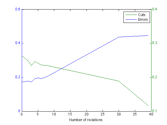
Figure 1: Influence of $\gamma$ on cut and clustering error.

It appears from a theoretical point of view that, due to noise, satisfying all constraints should not be the best choice. However, in our experiments it turned out, that typically the best results were achieved when all constraints were satisfied. We illustrate this behavior for the dataset Sonar, where we generated 80 constraints and increased $\gamma$ from zero until all constraints were satisfied. In Figure 1, we plot cuts and errors versus the number of violated constraints. One observes that the best error is obtained when all constraints were satisfied. Since by enforcing always all given constraints, our method becomes parameter-free (we increase $\gamma$ until all constraints are satisfied), we chose this option for the experiments.

5 Multi-Partitioning with Constraints

In this section we present a method to integrate constraints in a multi-partitioning setting. In the multi-partitioning problem, one seeks a $k$-partitioning $(C_{1},\ldots,C_{k})$ of the graph such that the normalized multi-cut given by

$$\sum_{i=1}^{k}\mathrm{NCut}(C_{i},\overline{C_{i}})$$ (6)

is minimized. A straightforward way to generate a multi-partitioning is to use a recursive bi-partitioning scheme. Starting with all points as the initial partition, the method repeats the following steps until the current partition has $k$ components.

1. split each of the components in the current partition into two parts.

2. choose among the above splits the one minimizing the multi-cut criterion.

Now we extend this method to the constrained case. Note that it is always possible to perform a binary split which satisfies all must-link constraints. Thus, must-link constraints pose no difficulty in the multi-partitioning scheme, as all must-link constraints can be integrated using the procedure given in 2.2.

However, satisfying all cannot-link constraints is sometimes not possible (cyclic constraints) and usually also not desirable at each level of the recursive bi-partition, since an early binary split cannot separate all classes. The issues here is which cannot-link constraints should be considered for the binary split in step 1.

To address this issue, we use the soft-version of our formulation where we need only to specify the maximum number, $l$, of violations allowed. We derive this number $l$ assuming the following simple uniform model of the data and constraints. We assume that all classes have equal size and there is an equal number of cannot link constraints between all pairs of classes. Assuming that any binary split does not destroy the class structure, the maximum number of violation is obtained if one class is separated from the rest. Precisely, the expected value of this number, given $N$ cannot-link constraints and $k$ classes, is $\frac{(k-1)(k-2)/2}{k(k-1)/2}\ N$. In the first binary split, these numbers ($N$ and $k$) are known. In the succesive binary splits, $N$ is known, while $k$ can again be derived, assuming the uniform model, as $\frac{k}{n}\ \tilde{n}$, where $\tilde{n}$ is the size of the current component.

We illustrate our approach using an artificial dataset (mixture of Gaussians, 500 points, 2 dimensions). Figure 2 shows on the left the ground truth and the solution of unconstrained ($\gamma$=0) multi-partitioning. In the unconstrained solution, points belonging to the same class are split into two clusters while points from other two classes are merged into a single cluster. On the rightmost, the result of our constrained multi-partitioning framework with 80 randomly generated constraints is shown.

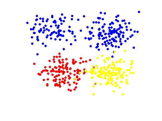
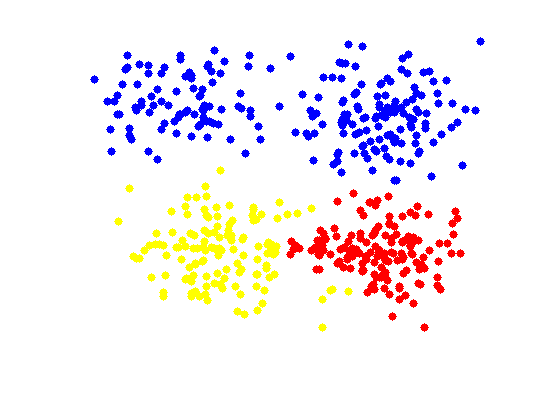
Figure 2: Left: ground-truth, middle: clustering obtained by unconstrained $1$-spectral clustering, right: clustering obtained by the constrained version.

6 Experiments

We compare our method against the following four related constrained clustering approaches: Spectral Learning (SL) [11], Flexible Constrained Spectral Clustering (CSP) [18], Constrained Clustering via Spectral Regularization (CCSR) [12] and Spectral Clustering with Linear Constraints (SCLC) [19]. SL integrates the constraints by simply modifying the weight matrix such that the edges connecting must-links have maximum weight and the edges of cannot-links have zero weight. CSP starts from the spectral relaxation and restricts the space of feasible solutions to those that satisfy a certain amount (specified by the user) of constraints. This amounts to solving a full generalized eigenproblem and choosing among the eigenvectors corresponding to positive eigenvalues the one that has minimum cost. CCSR addresses the problem of incorporating the constraints in the multi-class problem directly by an SDP which aims at adapting the spectral embedding to be consistent with the constraint information. For CSP and CCSR we use the code provided by the authors on their webpages.

In SCLC one solves the spectral relaxation of the normalized cut problem subject to linear constraints [5, 19]. Cannot-links and must-links are encoded via linear constraints as follows [5]: if the vertices $p$ and $q$ cannot-link (resp. must-link) then add a constraint $f_{p}=-f_{q}$ (resp. $f_{p}=f_{q}$). Although must-links are correctly formulated, one can argue that the encoding of cannot-links has modeling drawbacks. First observe that any solution that assigns zero to the constrained vertices $p$ and $q$ still satisfies the corresponding cannot-link constraint although it is not feasible to the constrained cut problem. Moreover, one can observe from the derivation of spectral relaxation [16], that vertices belonging to different components need to have only different signs but not the same value. Encoding cannot-links this way introduces bias towards partitions of equal volume, which can be observed in the experiments.

Our evaluation is based on three criteria: clustering error, normalized cut and fraction of constraints violated. For the clustering error we take the known labels and classify each cluster using majority vote. In this way each point is assigned a label and the clustering error is the error of this labeling. We use this measure as it is the expected error one would obtain when using simple semi-supervised learning, where one labels each cluster using majority vote.

The summary of the datasets considered is given in Table 1. The data with missing values are removed and the $k$-NN similarity graph is constructed from the remaining data as in [3].

Dataset	Size	Features	Classes
Sonar	208	60	2
Spam	4207	57	2
USPS	9298	256	10
Shuttle	58000	9	7
MNIST (Ext)	630000	784	10

Table 1: UCI datasets. The extended MNIST dataset is generated by translating each original input image of MNIST by one pixel, i.e., 8 directions.

In order to illustrate the performance in case of highly unbalanced problems, we create a binary problem (digit 0 versus rest) from USPS. The constraint pairs are generated in the following manner. We randomly sample pairs of points and for each pair, we introduce a cannot or must-link constraint based on the labels of the sampled pair. The results, averaged over $10$ trials are shown in Table 2 for 2-class problems and in Table 3 for multi-class problems. In the plots our method is denoted as COSC and we enforce always all constraints (see discussion in Section 4). Since our formulation is a non-convex problem, we use the best result (based on the achieved cut value) of 10 runs with random initializations. Except our method, no other method can guarantee to satisfy all constraints, even though SCLC does so in all cases. Our method produces always much better cuts than the ones found by SCLC which shows that our method is better suited for solving the constrained normalized cut problem. In terms of the clustering error, our method is consistently better than other methods. In case of unbalanced datasets (Spam, USPS 0 vs rest) our method significantly outperforms SCLC in terms of cuts and clustering error. Moreover, because of hard encoding of constraints, CSLC cannot solve multi-partitioning problems.

Table 2: Results for binary partitioning: Left: clustering error versus number of constraints, Middle: normalized cut versus number of constraints, Right: fraction of violated constraints versus number of constraints.

Table 3: Results for multi-partitioning - Left: clustering error versus number of constraints, Middle: normalized cut versus number of constraints, Right: fraction of violated constraints versus number of constraints.

6.1 Additional experimental results

Additional experimental results are given in Tables 5 and 6 for the datasets given in Table 4

Dataset	Size	Features	Classes
Breast Cancer	263	9	2
Heart	270	13	2
Diabetis	768	8	2
USPS	9298	256	10
MNIST	70000	784	10

Table 4: Additional UCI datasets

Table 5: Results for binary partitioning: Left: clustering error versus number of constraints, Middle: normalized cut versus number of constraints, Right: fraction of violated constraints versus number of constraints.

Table 6: Results for multi-partitioning - Left: clustering error versus number of constraints, Middle: normalized cut versus number of constraints, Right: fraction of violated constraints versus number of constraints.

References

- [1] S. Basu, I. Davidson, and K. Wagstaff. Constrained Clustering: Advances in Algorithms, Theory, and Applications. Chapman & Hall, 2008.
- [2] A. Beck and M. Teboulle. Fast gradient-based algorithms for constrained total variation image denoising and deblurring problems. IEEE Transactions on Image Processing, 18(11):2419–2434, 2009.
- [3] T. Bühler and M. Hein. Spectral clustering based on the graph p-Laplacian. In Proc. 26th Int. Conf. on Machine Learning (ICML), pages 81–88. Omnipress, 2009.
- [4] Tom Coleman, James Saunderson, and Anthony Wirth. Spectral clustering with inconsistent advice. In Proceedings of the 25th international conference on Machine learning, ICML ’08, pages 152–159, New York, NY, USA, 2008. ACM.
- [5] A.P. Eriksson, C. Olsson, and F. Kahl. Normalized cuts revisited: A reformulation for segmentation with linear grouping constraints. In IEEE 11th International Conference on Computer Vision (ICCV), pages 1–8, 2007.
- [6] Stephen Guattery and Gary L. Miller. On the quality of spectral separators. SIAM Journal on Matrix Analysis and Applications, 19:701–719, 1998.
- [7] L. W. Hagen and A. B. Kahng. Fast spectral methods for ratio cut partitioning and clustering. In Proc. Internat. Conf. on Computer Aided Design, pages 10–13, 1991.
- [8] M. Hein and T. Bühler. An inverse power method for nonlinear eigenproblems with applications in 1-spectral clustering and sparse PCA. In J. Lafferty, C. Williams, J. Shawe-Taylor, R. Zemel, and A. Culotta, editors, Advances in Neural Information Processing Systems 23 (NIPS), pages 847–855, 2010.
- [9] Matthias Hein and Simon Setzer. Beyond spectral clustering - tight relaxations of balanced graph cuts. In J. Shawe-Taylor, R.S. Zemel, P. Bartlett, F.C.N. Pereira, and K.Q. Weinberger, editors, Advances in Neural Information Processing Systems 24, pages 2366–2374. 2011.
- [10] J.-B. Hiriart-Urruty and C. Lemaréchal. Fundamentals of Convex Analysis. Springer, Berlin, 2001.
- [11] S.D. Kamvar, D. Klein, and C.D. Manning. Spectral learning. In Proc. of the 18th International Joint Conference On Artificial Intelligence (IJCAI), pages 561–566. Morgan Kaufmann, 2003.
- [12] Z. Li, J. Liu, and X. Tang. Constrained clustering via spectral regularization. In IEEE Conference on Computer Vision and Pattern Recognition (CVPR), pages 421–428, 2009.
- [13] R.T. Rockafellar. Convex analysis. Princeton University Press, 1970.
- [14] J. Shi and J. Malik. Normalized cuts and image segmentation. IEEE Trans. on Pattern Analysis and Machine Intelligence, 22:888–905, 2000.
- [15] A. Szlam and X. Bresson. Total variation and Cheeger cuts. In Proc. of the 27th International Conference on Machine Learning (ICML), pages 1039–1046. Omnipress, 2010.
- [16] U. von Luxburg. A tutorial on spectral clustering. Statistics and Computing, 17:395–416, 2007.
- [17] K. Wagstaff, C. Cardie, S. Rogers, and S. Schrödl. Constrained k-means clustering with background knowledge. In Proc. of the 18th International Conference on Machine Learning (ICML), pages 577–584. Citeseer, 2001.
- [18] X. Wang and I. Davidson. Flexible Constrained Spectral Clustering. In Proc. of the 16th ACM SIGKDD International conference on Knowledge Discovery and Data mining (KDD), pages 563–572. ACM Press, 2010.
- [19] L. Xu, W. Li, and D. Schuurmans. Fast normalized cut with linear constraints. In IEEE Conference on Computer Vision and Pattern Recognition (CVPR), pages 421–428, 2009.
- [20] S. X. Yu and J. Shi. Segmentation given partial grouping constraints. IEEE Trans. on Pattern Analysis and Machine Intelligence, 26:173–183, 2004.