Statistical equilibrium in deterministic cellular automata

Abstract

Some deterministic cellular automata have been observed to follow the pattern of the second law of thermodynamics: starting from a partially disordered state, the system evolves towards a state of equilibrium characterized by maximal disorder. This chapter is an exposition of this phenomenon and of a statistical scheme for its explanation. The formulation is in the same vein as Boltzmann’s ideas, but the simple combinatorial setup offers clarification and hope for generic mathematically rigorous results. Probabilities represent frequencies and subjective interpretations are avoided.

1 Introduction

The aim of statistical mechanics is to bridge between microscopic and macroscopic behaviour of systems consisting of a large number of interacting components. The prime example is a gas of particles moving and interacting according to the laws of mechanics, giving rise to macroscopic behaviour described in thermodynamics. The kinetic theory of gases, initiated by Clausius, Maxwell and Boltzmann, takes on the task of explaining the macroscopic behaviour of a gas on the basis of its microscopic description.

The main problem in kinetic theory is the derivation of the second law of thermodynamics (i.e., the tendency of an isolated thermodynamic system to evolve towards more disordered states). Starting from a collection of particles pictured as hard balls interacting through elastic collisions and using a simplifying (though erroneous) statistical assumption about the number of collisions of each type occurring in a small time interval (the Stosszahlansatz), Boltzmann was able to derive a version of the second law by showing that a certain quantity measuring disorder (Boltzmann’s entropy) increases monotonically with time and is maximized precisely when the system is in equilibrium.

Although the second law of thermodynamics was originally formulated for thermodynamic systems, its applicability goes beyond a system of particles following the particular laws of (classical or quantum) mechanics. A mathematical understanding of the precise circumstances leading to the applicability of the more general law of tendency towards disorder is desirable but missing.

The purpose of this chapter is to demonstrate examples of results and experimental observations regarding the so-called randomization behaviour in cellular automata (going back to Miyamoto, Wolfram and Lind) that could be thought of as instances of this generalized version of the second law of thermodynamics. Notably, neither probabilistic hypotheses (i.e., incorporating intrinsic randomness in the model) nor subjective interpretations (see Jay57 ) are needed — probabilities enter the picture only as intuitive means of representing statistical data. The combinatorial setting of cellular automata is simple enough that one could attempt to find generic mathematical conditions that guarantee the applicability of the second law. At the same time, the rich range of behaviour among cellular automata makes the challenge interesting and non-trivial.

The scenario is briefly as follows. Consider a configuration that is atypical of the maximally disordered state (so that there is a bias in the frequency of the patterns) but is not too rigidly regular either (e.g., it is not periodic). Over the time, a sufficiently chaotic cellular automaton shuffles such a configuration (albeit deterministically) in such a way that the bias gradually becomes undetectable. More specifically, the configuration of the system becomes more and more typical of the maximally disordered state, up to wider and wider ranges of observation.

2 Randomization Phenomenon: Examples

2.1 XOR cellular automaton

On the space of all bi-infinite sequences of symbols $\mathtt{0}$ and $\mathtt{1}$, consider a transformation $T$ that maps a sequence $x$ into another sequence $Tx$ defined by $(Tx)_{i}\triangleq x_{i}+x_{i+1}\pmod{2}$. In other words, $T$ replaces each symbol with the sum (modulo $2$) of that symbol and its right neighbour. The iteration of $T$ defines a dynamical system on $\{\mathtt{0},\mathtt{1}\}^{\mathbb{Z}}$, which we refer to as the XOR cellular automaton. Each sequence in $\{\mathtt{0},\mathtt{1}\}^{\mathbb{Z}}$ will be called a configuration of the system. A sample trajectory of this system is depicted in Figure 1.

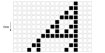
Figure 1: A sample trajectory of the XOR cellular automaton starting with a configuration consisting of a single $\mathtt{1}$ at the origin and $\mathtt{0}$ everywhere else.

The map $T$ is continuous with respect to the product topology. The product topology is the topology in which two configurations are considered “close” if they agree on a large region around the origin. Convergence in the product topology corresponds to site-wise eventual agreement. Another basic property of $T$ is its translation symmetries. Namely, if $\sigma^{k}$ denotes the translation by $k$ (that is, $(\sigma^{k}x)_{i}\triangleq x_{k+i}$), then $T\sigma^{k}=\sigma^{k}T$ for every $k\in\mathbb{Z}$. The map $T$ is also additive, meaning $T(x+y)=Tx+Ty$, where the addition is performed site-wise and modulo $2$. Although $T$ is not invertible, it is onto and “almost one-to-one” in that every configuration $y\in\{\mathtt{0},\mathtt{1}\}^{\mathbb{Z}}$ has precisely $2$ pre-images. Namely, choosing a symbol $x_{0}$ arbitrarily, we can find, recursively, unique values for the symbols $x_{i}$, for $i>0$ and $i<0$, such that $Tx=y$.

Slightly less obvious is the following balance property of $T$: if we choose the symbols in $x$ by independent unbiased coin flips, the symbols in $Tx$ will also be indistinguishable from independent unbiased coin flips. In other words, the uniform Bernoulli measure is invariant under $T$. To see this, take any block of $n$ consecutive symbols $b_{1}b_{2}\cdots b_{n}$ and consider the probability that $Tx$ takes values $b_{1}b_{2}\cdots b_{n}$ at positions $k$ to $k+n-1$. There are precisely two choices of values $a_{1}a_{2}\cdots a_{n+1}$ and $a^{\prime}_{1}a^{\prime}_{2}\cdots a^{\prime}_{n+1}$ that, if on $x$ at positions $k$ to $k+n$, lead to the desired values $b_{1}b_{2}\cdots b_{n}$ on $Tx$ at sites $k$ to $k+n-1$. Each of these two choices has probability $2^{-(n+1)}$ of appearing in independent flips of an unbiased coin. Therefore, $b_{1}b_{2}\cdots b_{n}$ appears at positions $k$ to $k+n-1$ of $Tx$ with probability $2^{-n}$.

Besides the balance property, the XOR cellular automaton has a wealth of other statistical regularities. For instance, if $x$ is chosen according to a uniform Bernoulli measure (i.e., with independent unbiased coin flips), then for any $n$, the sequence of blocks $(T^{t}x)_{[k,k+n)}$, $t=k,k+1,\ldots$ is independent of the block $x_{[k,k+n)}$. It follows from the law of large numbers that, almost surely, every pattern $a_{1}a_{2}\cdots a_{n}$ appears with the same frequency $2^{-n}$ in the space-time column $(T^{t}x)_{[k,k+n)}$, $t=0,1,2,\ldots$. The same sort of eventual independence holds along any other “space-time direction”: for every $a\in\mathbb{Z}^{+}$ and $b\in\mathbb{Z}$ and a sufficiently large $t_{0}$, the tilted column of blocks $(T^{at}x)_{[bt+k,bt+k+n)}$ with $t\geq t_{0}$ is independent of $x_{[k,k+n)}$.

Yet, the most remarkable property of the XOR cellular automaton for us is its randomization effect: if $x$ is chosen using independent flips of a biased coin (say, with probability $p\in(0,1)$ of having $\mathtt{1}$ at each site), then $T$ will gradually randomize $x$, meaning $T^{t}x$ will be asymptotically indistinguishable (in distribution) from a configuration chosen using independent flips of an unbiased coin as $t\to\infty$, provided we ignore a negligible set of time steps $t$ (Figure 2).

Figure 2: Randomization effect of the XOR cellular automaton. The starting configuration is chosen by independent biased coin flips with probability $p=0.1$ of having $\mathtt{1}$ at each site. Ignoring a negligible set of time steps (represented by gray lines), the configuration quickly becomes almost uniform.

To state this more precisely, we need some notation and terminology. A (Borel) probability measure on $\{\mathtt{0},\mathtt{1}\}^{\mathbb{Z}}$ is uniquely identified by the probabilities it associates to the cylinder sets

$$[a_{k}a_{k+1}\cdots a_{k+n}] \triangleq\{x\in\{\mathtt{0},\mathtt{1}\}^{\mathbb{Z}}:x_{k}x_{k+1}\cdots x_{k+n}=a_{k}a_{k+1}\cdots a_{k+n}\}\;.$$

For instance, for the Bernoulli measure with parameter $p$ (the distribution of independent flips of a biased coin with probability $p$ of having $\mathtt{1}$), which we will denote by $\mu_{p}$, we have

$$\mu_{p}([a_{k}a_{k+1}\cdots a_{k+n}]) =p^{\#_{\mathtt{1}}(a)}(1-p)^{\#_{\mathtt{0}}(a)}$$

for any block $a=a_{k}a_{k+1}\cdots a_{k+n}$, where $\#_{\mathtt{1}}(a)$ and $\#_{\mathtt{0}}(a)$ denote, respectively, the number of $\mathtt{1}$s and $\mathtt{0}$s appearing in $a$. The image of a probability measure $\pi$ under $T$ is another probability measure $T\pi$ with $(T\pi)(E)=\pi(T^{-1}E)$ for any measurable set $E$. This is the distribution of $Tx$ if $x$ is chosen at random according to $\pi$. A sequence of probability measures $\nu_{1},\nu_{2},\ldots$ is said to converge weakly to a measure $\pi$ if the probabilities that $\nu_{t}$ associate to each fixed cylinder converge to the probability of that cylinder according to $\pi$.

By the above-mentioned balance property, $T\mu_{1/2}=\mu_{1/2}$. Miyamoto Miy79 and Lind Lin84 (following experimental observations made by Wolfram Wol83 ) proved that

Theorem 2.1

There is a set $J\subseteq\mathbb{N}$ of density $1$ such that for every $p\in(0,1)$, $T^{t}\mu_{p}\to\mu_{1/2}$ as $t\to\infty$ within $J$.

Here, the density of a set of non-negative integers $J$ is defined as

$$d(J) \triangleq\lim_{n\to\infty}\frac{\left\lvert J\cap[0,n)\right\rvert}{n}$$

when the limit exists. The theorem in particular implies that the Cesàro averages $\frac{1}{n}\sum_{t=0}^{n-1}T^{t}\mu_{p}$ converge to $\mu_{1/2}$ as $n\to\infty$.

The randomization behaviour of the XOR cellular automaton can be seen as an analogue (or an instance) of the second law of thermodynamics: the system evolves towards an equilibrium in a macroscopic state with highest degree of disorder. Here, the term macroscopic is understood as synonymous with statistical: the macroscopic state of a configuration $x$ consists of the frequency of occurrence of every finite word $a\in\{\mathtt{0},\mathtt{1}\}^{*}$ in $x$. This information is encapsulated conveniently in a translation-invariant probability measure $\pi_{x}$ that is defined by those frequencies and which has $x$ as a “typical element”. The equilibrium state (the uniform Bernoulli measure) is the least presumptive (most random) state: every word of length $n$ has the same frequency $2^{-n}$. In Sections 3 and 4, we shall make this interpretation more precise.

The starting configuration does not need to be Bernoulli for the XOR cellular automaton to randomize it. A random configuration which is a realization of a (bi-infinite) $k$-step Markov chain with positive transition probabilities is also randomized by the XOR cellular automaton. In other words, the conclusion of Theorem 2.1 remains true if $\mu_{p}$ is replaced with a full-support Markov measure FerMaaMarNey00 . More generally, randomizaton is known to occur as long as the starting measure is harmonically mixing PivYas02 ; PivYas04 . A complete characterization of the measures randomized by the XOR map is nevertheless missing.

2.2 A reversible cellular automaton

The analogy with the second law of thermodynamics would have been stronger if the XOR cellular automaton were reversible or symmetric under time reversal. Consider now a different cellular automaton acting on the configurations of symbols from $S\triangleq\{\mathtt{0},\mathtt{1}\}\times\{\mathtt{0},\mathtt{1}\}$. Each site $i\in\mathbb{Z}$ of a configuration $(x,y)$ carries two symbols $x_{i}$ and $y_{i}$, and the cellular automaton map $T$ is defined by $\left(T(x,y)\right)_{i}\triangleq(y_{i},x_{i}+y_{i+1})$, where the addition is again modulo $2$. Let us call this the XOR-transpose cellular automaton. As in the XOR example, the map $T$ is continuous and translation-invariant. It is also additive and has the balance property: the uniform Bernoulli measure $\mu$ on $S^{\mathbb{Z}}$ is invariant under $T$. Unlike the XOR cellular automaton, the XOR-transpose is reversible and time-reversal symmetric: one can traverse backwards in time by switching the two symbols at each site. Maass and Martínez MaaMar99 proved that the XOR-transpose cellular automaton has a similar randomization property as the XOR cellular automaton (Figure 3):

Theorem 2.2

Let $\pi$ be the distribution of a single-step Markov chain on $S$ with positive transition probabilities. Then, $\frac{1}{n}\sum_{t=0}^{n-1}T^{t}\pi$ converges to the uniform Bernoulli measure $\mu$ as $n\to\infty$.

The convergence of the Cesàro averages implies the existence of a set $J\subseteq\mathbb{N}$ of density $1$ of time steps $t$ along which $T^{t}\pi$ converges to $\mu$ (see JohRud95 , Corollary 1.4), but the set $J$ might, in principle, depend on the measure $\pi$.

Figure 3: Randomization effect of the reversible cellular automaton of Maass and Martínez. In the initial configuration, each component of the symbol at each site is chosen with an independent coin flip with probability $0.1$ of having a $\mathtt{1}$.

2.3 A bi-permutative cellular automaton

As a third example, let us look at the cellular automaton with symbol set $S\triangleq\{\mathtt{0},\mathtt{1},\mathtt{2}\}$, defined by

$$(Tx)_{i}\triangleq\varphi(x_{i-1},x_{i},x_{i+1}) \triangleq\begin{cases}x_{i-1}+x_{i+1}+1\pmod{3}\quad&\text{if $x_{i}=\mathtt{2}$,}\\ x_{i-1}+x_{i+1}\pmod{3}&\text{otherwise.}\end{cases}$$ (1)

Unlike the last two examples, the map $T$ is not additive. Nevertheless, the local rule $\varphi$ is bi-permutative, which is to say both $a\mapsto\varphi(a,b,c)$ and $c\mapsto\varphi(a,b,c)$ are permutations. It follows, similarly as in the case of the XOR cellular automaton, that the map $T$ is $9$-to-$1$. Like the last two examples, the uniform Bernoulli measure (i.e., the distribution of a configuration chosen at random by flipping an unbiased “$3$-sided coin” independently for each site) is invariant under $T$. The bi-permutativity also ensures other statistical regularities for $T$, similar to those enjoyed by the XOR cellular automaton She92 .

It is not known whether the above cellular automaton has a randomizing behaviour in the sense of Theorems 2.1 or 2.2. Nevertheless, there is experimental evidence suggesting that $T$ indeed randomizes biased Bernoulli configurations (Figure 4). The graphs in Figure 4 depict the change in time of the empirical entropies of words of length $1$, $3$ and $7$ in consecutive configurations of this cellular automaton, starting from a biased Bernoulli configuration. More specifically, a single pseudo-random configuration $x$ is picked by simulating independent biased ($3$-sided) coin flips, and iterations of $T$ on $x$ are obtained for up to $50$ time steps. At each time step, the empirical entropy of words of length $k$ (for $k=1,3,7$) appearing in the current configuration are calculated as follows. For each word $w$ of length $k$ with symbols from $S$, let $\overline{\zeta_{w}}(y)$ denote the frequency of appearance of the word $w$ in configuration $y$. The empirical entropy of words of length $k$ appearing in $y$ is defined as

$$\hat{H}_{k}(y) \triangleq-\sum_{w\in S^{k}}\overline{\zeta_{w}}(y)\log\overline{\zeta_{w}}(y)\;.$$

Figure 4 shows that the empirical entropy $\hat{H}_{k}(T^{t}x)$ rapidly increases to reach its maximum at around $k\log 3$, where it stays.

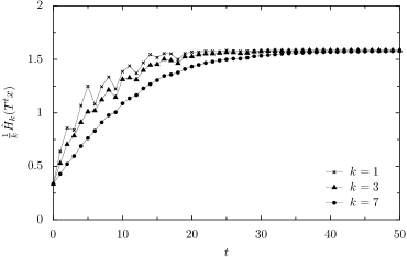
Figure 4: Evidence of randomization in the bi-permutative cellular automaton defined in Equation (1). The starting configuration $x$ (on a ring of length $50000$) is chosen with independent flips of a biased $3$-sided coin with distribution $(\mathtt{0}\mapsto 0.95,\mathtt{1}\mapsto 0.025,\mathtt{2}\mapsto 0.025)$.

The empirical entropy $\hat{H}_{k}(y)$ is a measure of disorder in $y$. It is maximized when all words of length $k$ appear in $y$ with approximately the same frequency. For instance, a configuration chosen using independent unbiased coin flips (which is considered to be maximally disordered) has, with probability $1$, the maximum empirical entropy $\hat{H}_{k}$ for each $k$. The empirical entropy $\hat{H}_{k}(y)$ should be compared with Boltzmann’s entropy (see below). Although not exhaustive, the simulation in Figure 4 suggests a gradual approach towards a maximally disordered state.

2.4 Rule 30

Yet another example where randomization seems to be present is the so-called Rule 30 cellular automaton. The Rule 30 cellular automaton has the binary alphabet $\{\mathtt{0},\mathtt{1}\}$ as the symbol set and may be defined by the logical expression

$$(Tx)_{i}\triangleq\varphi(x_{i-1},x_{i},x_{i+1}) \triangleq x_{i-1}\mathbin{\mathsf{XOR}}(x_{i}\mathbin{\mathsf{OR}}x_{i+1})\;,$$

where $\mathbin{\mathsf{XOR}}$ denotes “exclusive or”. The local rule $\varphi$ is not bi-permutative, but it is left-permutative (i.e., $a\leftrightarrow\varphi(a,b,c)$ is a bijection for each $b$ and $c$). This still implies that the map $T$ is onto, and that each configuration has at most $4$ pre-images under $T$. It follows that the Rule 30 cellular automaton again has the balance property. Starting from an unbiased Bernoulli configuration, the Rule 30 cellular automaton enjoys similar statistical regularities as in the previous examples, along almost all space-time directions She97 .

This cellular automaton was first studied by Wolfram Wol86 . He noticed that even with a simple starting configuration, the iterations of the Rule 30 cellular automaton produce complex seemingly unpredictable patterns. He proposed a method for generation of pseudo-random sequences by initializing the Rule 30 cellular automaton with a “seed” and picking the symbols appearing on a particular site every few time steps, which he tested against standard statistical randomness tests.

Figure 5 shows evidence for randomization in the Rule 30 cellular automaton starting from biased Bernoulli configurations. The empirical entropies are calculated as in the previous example.

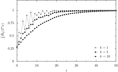
Figure 5: Evidence of randomization in the Rule 30 cellular automaton. The starting configuration $x$ (on a ring of length $50000$) is chosen with independent flips of a biased coin with probability $p=0.05$ of having a $\mathtt{1}$.

2.5 Q2R spin dynamics

One feature that is common among the first three examples (and is suspected for the Rule 30 cellular automaton) is the absence of conserved energy-like quantities ForKarTaa11 . A non-trivial conserved quantity would partition the macroscopic states into unescapable fibers, hence preventing complete randomization. Nevertheless, one might still expect randomization within each fiber.

The next example is based on the configurations of the Ising model, and was introduced by Vichniac Vic84 . The Ising model is a model of ferromagnetism: each site of an infinite two-dimensional square lattice (indexed by $\mathbb{Z}^{2}$) carries a symbol $\mathtt{\uparrow}$ or $\mathtt{\downarrow}$, representing two possible directions of a magnetic spin. The interaction between spins is modelled by assigning energy $-1$ or $+1$ to any pair of neighbouring sites whose symbols are, respectively, aligned or anti-aligned spins. The energy content of a region is the sum of the interaction energy of neighbouring sites in that region. Hence, lower energy in a region corresponds to an average tendency of neighbouring spins to be aligned.

The dynamics is through alternate applications of two maps $T_{0}$ and $T_{1}$: the first map updates the even sites (i.e., the sites $(i,j)$ with $i+j$ even) and the second updates the odd sites. The updating is done in such a way that the energy is preserved: a spin is flipped if and only if the flipping does not change the total energy of the site and its four immediate neighbours. More specifically, let us say that a site $(i,j)$ is balanced on a configuration $x$ if half of the neighbouring spins $x_{i+1,j}$, $x_{i,j+1}$, $x_{i-1,j}$ and $x_{i,j-1}$ are upward and the other half are downward. For a spin $a\in\{\mathtt{\uparrow},\mathtt{\downarrow}\}$, let $\overline{a}$ denote the spin with the opposite direction as $a$. Then,

$$(T_{0}x)_{i,j} \triangleq\begin{cases}\overline{x_{i,j}}\quad&\text{if $i+j$ even and $(i,j)$ balanced on $x$,}\\ x_{i,j}&\text{otherwise,}\end{cases}$$

and similarly for $T_{1}$. The dynamical system defined by the composition $T\triangleq T_{1}T_{0}$ is called the Q2R cellular automaton.

The Q2R system is reversible and symmetric under time reversal in the sense that $T^{-1}=T_{0}T_{1}$. By construction, it also conserves the energy. The conservation of energy can be formulated in various equivalent ways. For us, it suffices to say that $T$ (indeed, each of $T_{0}$ and $T_{1}$) keeps the average energy per site invariant. Note that the average energy per site of a configuration $x$ is a function of its macroscopic state $\pi_{x}$. The set of translation-invariant probability measures with a given average energy per site is convex and closed under the topology of weak convergence. Therefore, any limit or Cesáro limit of the measures $T^{t}\pi_{x}$ will have the same average energy per site as $\pi_{x}$.

As before, we consider the uniform Bernoulli measure on the configuration space $\{\mathtt{\uparrow},\mathtt{\downarrow}\}^{\mathbb{Z}^{2}}$ to be a representation of a “maximally disordered” state, because it assigns the same probability $2^{-\left\lvert A\right\rvert}$ to all cylinder sets

$$[q_{A}] \triangleq\{x\in\{\mathtt{\uparrow},\mathtt{\downarrow}\}^{\mathbb{Z}^{2}}:\text{$x_{i}=q_{i}$ for $i\in A$}\}\;.$$

Put another way, in a typical spin configuration obtained by independent unbiased coin flips, (translations of) each finite pattern $q_{A}:A\to\{\mathtt{\uparrow},\mathtt{\downarrow}\}$ appears with the same frequency $2^{-\left\lvert A\right\rvert}$. Another way to express this is to say that the entropy

$$H_{A}(\mu) \triangleq-\sum_{q_{A}:A\to\{\mathtt{\uparrow},\mathtt{\downarrow}\}}\mu([q_{A}])\log\mu([q_{A}])$$

of any finite window $A\subseteq\mathbb{Z}^{2}$ has its maximum value $\left\lvert A\right\rvert\log 2$ if $\mu$ is the uniform Bernoulli measure.

The description of a “maximally disordered” state with a given average energy per site is more subtle. Indeed, since the constraint is not local, it might not be possible to maximize the entropy $H_{A}(\mu)$ simultaneously for all finite windows $A$. However, if $B\supseteq A$, a larger value for $H_{B}(\mu)$ is a better indication of disorder than a larger value for $H_{A}(\mu)$. Therefore, one may measure the disorder by the limit entropy per site

$$h(\mu) \triangleq\lim_{n\to\infty}\frac{H_{I_{n}}(\mu)}{\left\lvert I_{n}\right\rvert}\;,$$

where $I_{n}=[-n,n]\times[-n,n]$. A maximally disordered state with a given average energy per site may therefore be identified with an ergodic translation-invariant measure that has the prescribed average energy per site and maximal entropy per site subject to the energy constraint. These are the ergodic Gibbs measures for the Ising model (see e.g. Rue04 ; Isr79 ).

Figure 6 shows few snapshots from a simulation of the Q2R cellular automaton starting from a biased Bernoulli configuration. At the beginning, the spins gradually cluster, even though the total length of the boundaries between upward and downward clusters remains constant. After a while, the macroscopic picture of the configuration appears to reach an equilibrium, which resembles a typical configuration chosen according to a Gibbs measure of the Ising model. More elaborate simulations have shown numerical agreement with the Ising model (see e.g. Her86 ; TofMar87 ), hence supporting the conjecture that Q2R indeed randomizes a coin-flip configurations within the corresponding average energy per site level.

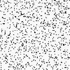
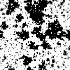
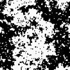
t=0		t=500		t=5000

Figure 6: Simulation of the Q2R cellular automaton starting from a coin-flip configuration with probability $p=0.1$ of having $\mathtt{\uparrow}$ (represented by black). After a relatively short while, the macroscopic look of the configuration seems to reach an equilibrium with upward and downward spins clustered together.

In the next two sections, we attempt to make the concepts of macroscopic state and maximally disordered state more precise.

3 Macroscopic States

Let us fix a symbol set $S$ and denote by $\mathcal{X}=\{x:\mathbb{Z}^{d}\to S\}$ the set of all $d$-dimensional configurations of symbols from $S$. A configuration $x\in\mathcal{X}$ is considered as a microscopic state of a system. The macroscopic state of $x$ consists of all information in $x$ that is visible through “macroscopic observations”. Which observations are considered macroscopic is somewhat arbitrary and depends on the physical context. Here, we equate “macroscopic” with “statistical”: a macroscopic observation would amount to identifying the frequency of a fixed pattern, or the spatial average of a “microscopic observation”.

To be more specific, let us call a function $f:\mathcal{X}\to\mathbb{R}$ a local observable if the symbols $x_{i}$ at finitely many sites $i\in A$ are sufficient to determine $f(x)$. For instance, if $q:A\to S$ is a pattern on a finite set $A$, the function $x\mapsto\zeta_{q}(x)$ that has value $1$ if $x$ agrees with $q$ on $A$ and $0$ otherwise is a local observable. Furthermore, any local observable is a linear combination of observables of this type.

If $f$ is a local observable, the spatial average

$$\overline{f}(x) \triangleq\lim_{n\to\infty}\frac{1}{\left\lvert I_{n}\right\rvert}\sum_{i\in I_{n}}f(\sigma^{i}x)$$ (2)

will be considered as a macroscopic observable. As before, $I_{n}\triangleq[-n,n]^{d}$, and $\sigma^{i}$ denotes the translation by $i$. For instance, $\overline{\zeta_{q}}(x)$ is simply the frequency of the occurrence of (translations of) the pattern $q$ in $x$. The limit in (2) may or may not exist. If well-defined, the collection $\left(\overline{f}(x):\text{$f$ local}\right)$ defines a unique translation-invariant probability measure $\pi_{x}$ with

$$\pi_{x}(f)=\int f\mathrm{d}\pi_{x} =\overline{f}(x)\;,$$

describing the statistics of $x$. In particular, $\pi_{x}([q])=\overline{\zeta_{q}}(x)$ for any finite pattern $q$.

Every translation-invariant probability measure on $\mathcal{X}$ arises from a configuration in the above fashion Oxt63 . Nevertheless, not every translation-invariant probability measure should be considered as an unambiguous macroscopic state. To illustrate this, consider a one-dimensional configuration $z$ with $z_{i}=\mathtt{0}$ for $i<0$ and $z_{i}=\mathtt{1}$ for $i>0$. Then $\pi_{z}=\frac{1}{2}(\delta_{\underline{\mathtt{0}}}+\delta_{\underline{\mathtt{1}}})$, where $\delta_{\underline{\mathtt{0}}}$ and $\delta_{\underline{\mathtt{1}}}$ are the point-mass measures at the uniform configurations $\underline{\mathtt{0}}$ and $\underline{\mathtt{1}}$. The measure $\frac{1}{2}(\delta_{\underline{\mathtt{0}}}+\delta_{\underline{\mathtt{1}}})$ however suggests an ambiguous situation in which we are uncertain about which of $\underline{\mathtt{0}}$ and $\underline{\mathtt{1}}$ is the real configuration of the system. The ambiguity comes from the fact that the configuration $z$ lacks homogeneity: its left and right tails have different macroscopic looks.

Here, we focus on configurations that are homogeneous. We call a configuration $x$ homogeneous if

1. $\pi_{x}$ is well-defined (i.e., the spatial average $\overline{f}(x)$ of every local observable $f$ exists on $x$),

2. $\pi_{x}$ cannot be written as a non-trivial convex combination of other translation-invariant measures (i.e., $\pi_{x}$ is ergodic for the group of translations), and

3. $x$ is a point of density for $\pi_{x}$, which is to say, every finite pattern occurring in $x$ occurs with positive frequency.

The measure $\pi_{x}$ describing the statistical averages of a homogeneous configuration $x$ will be called the macroscopic state of $x$. The set of homogeneous configurations sharing the same ergodic measure $\pi$ as macroscopic state is called the ergodic set of $\pi$. The countability of the set of finite patterns together with the ergodic theorem implies that the ergodic set of any ergodic measure $\pi$ has measure $1$ with respect to $\pi$ (see Oxt52 ). Hence, one may think of a configuration in the ergodic set of $\pi$ as a typical configuration with macroscopic state $\pi$.

4 Maximally Disordered States

From the definition, it follows that, for any finite window $A\subseteq\mathbb{Z}^{d}$, the entropy $H_{A}(\pi)$ of a macroscopic state (i.e., a translation-ergodic measure) $\pi$ agrees with the empirical entropy $\hat{H}_{A}(x)$ of any configuration $x$ that is typical for $\pi$. The entropy $H_{A}(\pi)$ is a convex continuous function of $\pi$, taking its maximum value $\left\lvert A\right\rvert\log\left\lvert S\right\rvert$ only when $\pi$ assigns equal probabilities to every cylinder with base $A$.

The limit entropy per site $h(\pi)$ is affine (hence convex) and takes its maximum value $\log\left\lvert S\right\rvert$ precisely when $\pi$ is the uniform Bernoulli measure, that is the state with “maximum disorder”. The map $\pi\mapsto h(\pi)$ is however not continuous. For example, for each $m>0$, let $x(m)$ be a periodic configuration in $\{\mathtt{0},\mathtt{1}\}^{\mathbb{Z}}$ that has each word of length $m$ exactly once in its period. Then, the macroscopic states $\pi_{x(m)}$ have $0$ entropy per site yet converge weakly to the uniform Bernoulli measure as $m\to\infty$. In fact, every macroscopic state is a weak limit of macroscopic states of periodic configurations (which all have entropy $0$). Nevertheless, entropy per site is upper semi-continuous: $\pi_{n}\to\pi$ implies $\limsup_{n\to\infty}h(\pi_{n})\leq h(\pi)$ (see e.g. Wal82 ).

Let us now consider a concept of energy as in the Ising model. Namely, let $f:\mathcal{X}\to\mathbb{R}$ be a local observable, representing the energy contribution of the symbol at the origin when interacting with the nearby symbols. For instance, for the Ising model, we can set

$$f(x) =\begin{cases}\frac{1}{2}\left(n_{\mathtt{\downarrow}}(\partial_{0}x)-n_{\mathtt{\uparrow}}(\partial_{0}x)\right)\quad&\text{if $x_{0}=\mathtt{\uparrow}$,}\\ \frac{1}{2}\left(n_{\mathtt{\uparrow}}(\partial_{0}x)-n_{\mathtt{\downarrow}}(\partial_{0}x)\right)&\text{if $x_{0}=\mathtt{\downarrow}$,}\end{cases}$$

where $n_{\mathtt{\uparrow}}(\partial_{0}x)$ and $n_{\mathtt{\downarrow}}(\partial_{0}x)$ are the numbers of upward and downward spins among the four neighbours $x_{1,0}$, $x_{0,1}$, $x_{-1,0}$ and $x_{0,-1}$ of site $0$. Then, $\overline{f}(x)$ represents the average energy per site of a configuration $x$, which is well-defined if $x$ is homogeneous, and agrees with $\pi_{x}(f)$.

Suppose $e$ is a real number within the range of $\overline{f}$. Among all the macroscopic states $\pi$ satisfying $\pi(f)=e$, those with maximum entropy per site $h(\pi)$ could be considered as the most disordered. These are the presumed equilibrium states of a system in which the energy $f$ is conserved. Applying the Lagrange multipliers method (Legendre transform), the optimization problem

maximize $$h(\pi)$$

subject to $$\pi(f)=e$$

(for $e$ in the range of $\overline{f}$) translates into the unconstrained problem

maximize $$h(\pi)-\beta\pi(f)$$ (3)

(for $\beta\in\mathbb{R}$). The compactness of the space, the continuity of $\pi\mapsto\pi(f)$ and the upper semi-continuity of $\pi\mapsto h(\pi)$ imply that, in both problems, the maximums are achieved by some translation-invariant probability measures. Dobrushin, Lanford and Ruelle proved that the macroscopic states solving the variational problem (3) are precisely the ergodic Gibbs measures at inverse temperature $\beta$. See Rue04 ; Isr79 ; Kel98 for more information.

5 Boltzmann’s Theory and Cellular Automata

Let us take a moment to draw parallels between the concepts in Boltzmann’s gas theory and in cellular automata. We refer to the survey article of the Ehrenfests EhrEhr12 and the book by Kac Kac59 , which contain excellent accounts of Boltzmann’s theory and related issues. See also Leb99 for a general discussion.

Boltzmann considered an isolated collection of $n$ particles (identical hard spheres) interacting via elastic collisions. The particles are assumed to be homogeneously distributed in (a bounded but large region of) the space. To be concrete, we may consider a cubic region with periodic boundary conditions. The focus is thus only on the velocity of the particles. Assuming that the number of particles is very large, we take $\rho(v,t)\mathrm{d}v$ to be the fraction of particles that, at time $t$, have velocities within an infinitesimal approximation $\mathrm{d}v$ of each value $v\in\mathbb{R}^{3}$. Using the assumption of spatial homogeneity, Boltzmann estimated the average number of collisions, in an infinitesimally small time interval $(t,t+\mathrm{d}t)$, among particles with velocities close to $u$ and those with velocities close to $v$ (the Stosszahlansatz). The model of elastic collisions (the conservation of energy and momentum) could now be invoked to obtain the new distribution $\rho(v,t+\mathrm{d}t)\mathrm{d}v$ for the velocity of the particles at the end of the time interval $(t,t+\mathrm{d}t)$. This leads to an equation describing the time evolution of $\rho(v,t)$ known as the Boltzmann equation. Boltzmann used this equation to show that the quantity $-\int\rho(v,t)\log\rho(v,t)\mathrm{d}v$ is monotonically increasing in time, except at an equilibrium in which the velocities are distributed according to the Maxwell distribution $\rho(v)\sim\mathrm{e}^{-c\left\lvert v\right\rvert^{2}}$.

Boltzmann’s derivation of the “law of increase in entropy” faced two major criticisms. Loschmidt objected that a system governed by a reversible and time-reversal symmetric dynamics (like a system of particles interacting via elastic collisions) cannot possibly have an observable that is invariant under time reversal (like entropy) and is monotonically increasing in all situations. Zermelo’s objection was based on Poincaré’s recurrence theorem. According to Liouville’s theorem, a Hamiltonian system (such as a system of particles) preserves the phase space volume (i.e., the Lebesgue measure). Poincaré’s theorem states that in a volume-preserving system whose phase-space has finite volume (such as an isolated system of particles in a $3$-dimensional torus), almost every trajectory eventually returns (infinitely many times) arbitrarily close to its starting point. This again implies that such a system cannot have a continuous observable that is monotonically increasing in time for almost all starting points.

In order to address these criticisms, Boltzmann later introduced another more refined framework. In this new setting, each particle $i$ is described by a state variable $x_{i}$, which could, for instance, consist of the position as well as the velocity of the particle. The phase space of an individual particle (i.e., the range of values of $x_{i}$) is divided into small equally-sized regions $A_{1},A_{2},\ldots$. Given a configuration of particles $x$, we can form the fraction $\rho_{k}=n_{k}/n$ of particles whose states are in region $A_{k}$. Conversely, given the macroscopic information $\rho=(\rho_{1},\rho_{2},\ldots)$, there corresponds a set $[\rho]$ consisting of all particle configurations that have fractions $\rho_{1},\rho_{2},\ldots$ of particles in regions $A_{1},A_{2},\ldots$. If the number of particles is very large, the volume of the set $[\rho]$ could be measured by the quantity $H(\rho)=-\sum_{k}\rho_{k}\log\rho_{k}$. Neglecting any interaction energy between particles, the energy of a configuration $x$ could be written as $E(x)=n\sum_{k}\rho_{k}e_{k}$, where $e_{k}$ is the (approximate) energy of a particle whose state is within $A_{k}$. Boltzmann now argued that a system with energy $E$ at equilibrium is most likely to be found (at almost any moment of time) to have a state distribution $\rho$ that maximizes the quantity $H(\rho)$ among all the state distributions with energy $E$, for this is the distribution for which $[\rho]$ takes the overwhelmingly largest portion of the set of all configurations with energy $E$. If $n$ is large, this equilibrium distribution is (approximately) given by $\rho_{k}\sim\mathrm{e}^{-\beta e_{k}}$, where $\beta$ is a Lagrange multiplier for tuning $E$.

The analogy with cellular automata should be clear. Rather than particles, the elementary pieces of information in cellular automata are carried by lattice sites representing discretized positions in the space. The symbol at site $i$ should therefore be compared with the state of particle $i$. The model of elastic collisions governing the interaction between the particles is replaced with the local update rule describing the cellular automaton map $T:S^{\mathbb{Z}^{d}}\to S^{\mathbb{Z}^{d}}$. The fraction $\overline{\zeta_{a}}(x)$ of sites having symbol $a$ is an elementary macroscopic observable analogous to the fraction $n_{k}/n$ of particles whose states are in region $A_{k}$, but now it is clear that one must also take into account the macroscopic observables $\overline{\zeta_{q}}(x)$ (for larger patterns $q:A\to S$) which contain information about correlations between finite collections of sites. Boltzmann’s entropy corresponds to the empirical entropy $\hat{H}_{0}(x)$ of symbols appearing in the configuration $x$, or more generally, the empirical entropy $\hat{H}_{A}(x)$, which measures lack of bias in the frequency of the patterns with support $A$ occurring in $x$.

To understand Boltzmann’s argument about the increase in entropy, consider the XOR cellular automaton (Section 2.1), and let $x$ be a Bernoulli random configuration with parameter $p\in(0,1)$ (i.e., a homogeneous configuration whose macroscopic state is described by the Bernoulli measure with parameter $p$). In particular, the words of length $2$ have frequencies

$$\overline{\zeta_{\mathtt{0}\mathtt{0}}}(x) =(1-p)^{2}\;, \overline{\zeta_{\mathtt{0}\mathtt{1}}}(x) =(1-p)p\;, \overline{\zeta_{\mathtt{1}\mathtt{0}}}(x) =p(1-p)\;, \overline{\zeta_{\mathtt{1}\mathtt{1}}}(x) =p^{2}$$

in $x$. It follows that the frequency $\overline{\zeta_{\mathtt{1}}}(Tx)$ of occurrence of symbol $\mathtt{1}$ after one step is $\varphi(p)\triangleq 2p(1-p)$. If $\mathsf{H}(p)\triangleq-p\log p-(1-p)\log(1-p)$ denotes the binary entropy function, one can easily verify that $\mathsf{H}(\varphi(p))\geq\mathsf{H}(p)$ with equality if and only if $p=\frac{1}{2}$. Therefore, it is indeed the case that the entropy $\hat{H}_{0}(Tx)$ is larger than $\hat{H}_{0}(x)$ unless $p=\frac{1}{2}$.

Boltzmann’s assumption about the number of collisions (the Stosszahlansatz) is analogous to the (invalid) assumption that the configuration $Tx$ is also Bernoulli, so that the frequency of occurrence of a word $w=a_{1}a_{2}\cdots a_{n}$ in $Tx$ is simply the product of the frequencies of $a_{1},a_{2},\ldots,a_{n}$. If true, this would lead to the conclusion that the entropy increases monotonically in the consecutive steps, that is, $H_{0}(x)\leq H_{0}(Tx)\leq H_{0}(T^{2}x)\leq\cdots$ with the equalities only if $H_{0}(x)=\log 2$. The assumption is of course false. Nevertheless, the randomization property of the XOR cellular automaton (Theorem 2.1) suggests a mathematically rigorous scenario that makes Boltzmann’s conclusion essentially true. Indeed, the randomization implies that for any finite set $A\subseteq\mathbb{Z}$, the entropy $\hat{H}_{A}(T^{t}x)$ approaches (after ignoring a negligible set of time steps) to its maximum value $\left\lvert A\right\rvert\log 2$, even if this convergence might be non-monotonic.

For cellular automata, the uniform Bernoulli measure plays the role of the Lebesgue measure on the phase space of a Hamiltonian system. The analog of Liouville’s theorem is the balance property, which says that any surjective cellular automaton map $T:S^{\mathbb{Z}^{d}}\to S^{\mathbb{Z}^{d}}$ preserves the uniform Bernoulli measure. Hence, Poincaré’s theorem applies to all surjective cellular automata. It says that starting from almost every configuration $x$ (i.e., any configuration in a set of uniform Bernoulli measure $1$), every finite pattern occurring on $x$ (i.e., $q=x_{A}$ for some finite set $A\subseteq\mathbb{Z}^{d}$) reappears on the same position infinitely many times (i.e., $(T^{t}x)_{A}=q$ for infinitely many time steps $t$). Note that this does not say anything about a starting configuration that is not typical for the uniform Bernoulli measure.

It is worth mentioning that surjective cellular automata preserve the limit entropy per site, that is, $h(T^{t}\pi)=h(\pi)$ for every macroscopic state $\pi$ and $t=1,2,\ldots$ (see e.g. KarTaa14 ). On the other hand, randomization implies a jump at the limit to $h(\mu)>\lim_{\begin{subarray}{c}t\in J\\ t\to\infty\end{subarray}}h(T^{t}\pi)=h(\pi)$. This may be understood as follows. A sub-maximum value for $H_{A}(\pi)$ expresses the presence of correlations among symbols with relative positions given by $A$. The convergence of the entropy $H_{A}(T^{t}\pi)$ to its maximal value $\left\lvert A\right\rvert\log\left\lvert S\right\rvert$ for larger and larger finite sets $A\subseteq\mathbb{Z}^{d}$ indicates that the correlations are gradually distributed over larger and larger regions, and are escaping to infinity as $t$ grows to infinity.

6 How Far the Second Law Goes?

The phenomenon described by the second law of thermodynamics extends to all physical systems. What constitutes a physical system and what is the exact statement of the second law are much less clear. Let us discuss few prerequisites for the presence of the randomization effect. For simplicity, we focus on the case that the cellular automaton has no non-trivial conserved quantity.

To fix the terminology, let us say that a cellular automaton $T:S^{\mathbb{Z}^{d}}\to S^{\mathbb{Z}^{d}}$ randomizes a translation-invariant probability measure $\pi$ if the Cesàro averages $\frac{1}{n}\sum_{t=0}^{n-1}T^{t}\pi$ converge weakly to the uniform Bernoulli measure $\mu$ as $n$ goes to infinity. Equivalently, $T$ randomizes $\pi$ if $T^{t}\pi\to\mu$ along a subsequence $J\subseteq\mathbb{N}$ of density $1$ of time steps (see JohRud95 , Corollary 1.4).

An obvious case in which randomization fails is when $T$ is not surjective. Lack of surjectivity (or reversibility) has been suggested as a mechanism behind the contrasting phenomenon of self-organization (see e.g. Wol83 ). The requirement for $T$ to be surjective is a relaxation compared to reversibility (let alone time-reversal symmetry), which is common among most microscopic physical theories. Yet, surjectivity already guarantees the invariance of the uniform Bernoulli measure. Moreover, surjective cellular automata are in some way close to being injective: if two configurations $x,y$ differ on at most finitely many positions, then $Tx$ and $Ty$ are distinct (see e.g. Kar05 ).

Besides surjectivity, the cellular automaton requires to have certain degree of chaos in order for randomization to occur. For instance, for a one-dimensional surjective cellular automata with equicontinuity points, the Cesàro averages $\frac{1}{n}\sum_{t=0}^{n-1}T^{t}\pi$ with a Bernoulli starting measure $\pi$ converge but not necessarily to the uniform Bernoulli measure BlaTis00 . Such cellular automaton typically have too many distinct conserved quantities, resulting in failure of any thermodynamic behaviour (see Tak87 ; KarTaa14 ).

Another obstacle for randomization is too much regularity in the starting configuration. The simplest type of regularity is periodicity. Note that a spatially periodic configuration is also temporally periodic. Therefore, no cellular automaton can randomize a periodic configuration. A spatially periodic configuration has zero entropy per site. As a more sophisticated example of a regularity obstructing randomization, consider the XOR cellular automaton. The XOR cellular automaton has the following self-similarity property, which can be verified by induction: $(T^{2^{n}}x)_{i}=x_{i}+x_{i+2^{n}}\pmod{2}$ for every $n\geq 0$. Define the duplicate of a configuration $x$ as the configuration $Dx$ with $(Dx)_{2i}\triangleq(Dx)_{2i+1}\triangleq x_{i}$. It follows from self-similarity that $DTx=T^{2}Dx$, or more generally $D^{n}Tx=T^{2^{n}}D^{n}x$. For the uniform Bernoulli measure $\mu$, in particular, we find that $T^{2^{n}}D^{n}\mu=D^{n}\mu$. Note that if $\pi$ is a translation-ergodic measure, the measure $\overline{D}\pi\triangleq\frac{1}{2}(D\pi+\sigma D\pi)$ is also translation-ergodic and has entropy per site $\frac{1}{2}h(\pi)$. Moreover, if $T^{k}\pi=\pi$, we get $T^{2k}\overline{D}\pi=\overline{D}\pi$. Therefore, we have an infinite sequence $\overline{D}\mu,\overline{D}^{2}\mu,\overline{D}^{3}\mu,\ldots$ of distinct translation-ergodic measures (i.e., macroscopic states) with positive entropy that are not randomized by the XOR cellular automaton.

In summary, randomization is expected only if the cellular automaton is surjective and “sufficiently chaotic”, and the starting configuration does not have “too much regularity”.

- (1) Blanchard, F., Tisseur, P.: Some properties of cellular automata with equicontinuity points. Annales de l’Institut Henri Poincaré, Probabilités et Statistiques 36(5), 569–582 (2000)
- (2) Cercignani, C., Illner, R., Pulvirenti, M.: The Mathematical Theory of Dilute Gases. Springer-Verlag (1994)
- (3) Cover, T.M., Thomas, J.A.: Elements of Information Theory. Wiley (1991)
- (4) Ehrenfest, P., Ehrenfest, T.: The Conceptual Foundations of the Statistical Approach in Mechanics. Cornell University Press (1959). Originally appeared in 1912 as volume IV, part 32 of the Encyklopädie der mathematischen Wissenschaften.
- (5) Einsiedler, M.: Invariant subsets and invariant measures for irreducible actions on zero-dimensional groups. Bulletin of the London Mathematical Society 36(3), 321–331 (2004)
- (6) Ferrari, P.A., Maass, A., Martínez, S., Ney, P.: Cesàro mean distribution of group automata starting from measures with summable decay. Ergodic Theory and Dynamical Systems 20(6), 1657–1670 (2000)
- (7) Formenti, E., Kari, J., Taati, S.: On the hierarchy of conservation laws in a cellular automaton. Natural Computing 10(4), 1275–1294 (2011)
- (8) Gajardo, A., Kari, J., Moreira, A.: On time-symmetry in cellular automata. Journal of Computer and System Sciences 78(4), 1115–1126 (2012)
- (9) Georgii, H.O.: Gibbs Measures and Phase Transitions. Walter de Gruyter (1988)
- (10) Georgii, H.O.: Probabilistic aspects of entropy. In: A. Greven, G. Keller, G. Warnecke (eds.) Entropy, pp. 37–54. Princeton University Press (2003)
- (11) Hedlund, G.A.: Endomorphisms and automorphisms of the shift dynamical system. Mathematical System Theory 3, 320–375 (1969)
- (12) Herrmann, H.J.: Fast algorithm for the simulation of Ising models. Journal of Statistical Physics 45(1/2), 145–151 (1986)
- (13) Host, B., Maass, A., Martínez, S.: Uniform bernoulli measure in dynamics of permutative cellular automata with algebraic local rules. Discrete and Continuous Dynamical Systems — Series A 9(6), 1423–1446 (2003)
- (14) Israel, R.B.: Convexity in the theory of lattice gases. Princeton University Press (1979)
- (15) Jaynes, E.T.: Information theory and statistical mechanics. The Physical Review 106(4), 620–630 (1957)
- (16) Johnson, A., Rudolph, D.J.: Convergence under of invariant measures on the circle. Advances in Mathematics 115(1), 117–140 (1995)
- (17) Kac, M.: Probability and Related Topics in Physical Sciences. Interscience Publishers (1959)
- (18) Kari, J.: Theory of cellular automata: A survey. Theoretical Computer Science 334, 3–33 (2005)
- (19) Kari, J., Taati, S.: Statistical mechanics of surjective cellular automata. Journal of Statistical Physics (To appear). [arXiv:1311.2319]
- (20) Keller, G.: Equilibrium States in Ergodic Theory. Cambridge University Press (1998)
- (21) Kůrka, P.: Topological and Symbolic Dynamics, Cours Spécialisés, vol. 11. Société Mathématique de France (2003)
- (22) Lanford III, O.E.: Time evolution of large classical systems. In: J. Moser (ed.) Dynamical Systems, Theory and Applications, Lecture Notes in Physics, vol. 38, pp. 1--111 (1975)
- (23) Lebowitz, J.L.: Statistical mechanics: A selective review of two central issues. Reviews of Modern Physics 71(2) (1999)
- (24) Lind, D.A.: Applications of ergodic theory and sofic systems to cellular automata. Physica D: Nonlinear Phenomena 10(1--2) (1984)
- (25) Maass, A., Martínez, S.: Time averages for some classes of expansive one-dimensional cellular automata. In: Cellular Automata and Complex Systems, Nonlinear Phenomena and Complex Systems, vol. 3, pp. 37--54. Kluwer Academic Publishers (1999)
- (26) Miyamoto, M.: An equilibrium state for a one-dimensional life game. Journal of Mathematics of Kyoto University 19, 525--540 (1979)
- (27) Oxtoby, J.C.: Ergodic sets. Bulletin of the American Mathematical Society 58(2), 116--136 (1952)
- (28) Oxtoby, J.C.: On two theorems of Parthasarathy and Kakutani concerning the shift transformation. In: F.B. Wright (ed.) Ergodic Theory, pp. 203–--215. Academic Press (1963)
- (29) Pivato, M., Yassawi, R.: Limit measures for affine cellular automata. Ergodic Theory and Dynamical Systems 22, 1269--1287 (2002)
- (30) Pivato, M., Yassawi, R.: Limit measures for affine cellular automata II. Ergodic Theory and Dynamical Systems 24, 1961--1980 (2004)
- (31) Ruelle, D.: Thermodynamic Formalism, second edn. Cambridge University Press (2004)
- (32) Shereshevsky, M.A.: Ergodic properties of certain surjective cellular automata. Monatshefte für Mathematik 114(3--4), 305--316 (1992)
- (33) Shereshevsky, M.A.: K-property of permutative cellular automata. Indagationes Mathematicae 8(3), 411--416 (1997)
- (34) Takesue, S.: Reversible cellular automata and statistical mechanics. Physical Review Letters 59(22), 2499--2502 (1987)
- (35) Toffoli, T., Margolus, N.: Cellular Automata Machines: A New Environment for Modeling. MIT Press (1987)
- (36) Vichniac, G.Y.: Simulating physics with cellular automata. Physica D 10, 96--116 (1984)
- (37) Walters, P.: An Introduction to Ergodic Theory. Springer-Verlag (1982)
- (38) Wolfram, S.: Statistical mechanics of cellular automata. Reviews of Modern Physics 55, 601--644 (1983)
- (39) Wolfram, S.: Random sequence generation by cellular automata. Advances in Applied Mathematics 7, 123--169 (1986)