Parameter-free Topology Inference and Sparsification for Data on Manifolds

Abstract

In topology inference from data, current approaches face two major problems. One concerns the selection of a correct parameter to build an appropriate complex on top of the data points; the other involves with the typical ‘large’ size of this complex. We address these two issues in the context of inferring homology from sample points of a smooth manifold of known dimension sitting in an Euclidean space $\mathbb{R}^{k}$. We show that, for a sample size of $n$ points, we can identify a set of $O(n^{2})$ points (as opposed to $O(n^{\lceil\frac{k}{2}\rceil})$ Voronoi vertices) approximating a subset of the medial axis that suffices to compute a distance sandwiched between the well known local feature size and the local weak feature size (in fact, the approximating set can be further reduced in size to $O(n)$). This distance, called the lean feature size, helps pruning the input set at least to the level of local feature size while making the data locally uniform. The local uniformity in turn helps in building a complex for homology inference on top of the sparsified data without requiring any user-supplied distance threshold. Unlike most topology inference results, ours does not require that the input is dense relative to a global feature such as reach or weak feature size; instead it can be adaptive with respect to the local feature size. We present some empirical evidence in support of our theoretical claims.

1 Introduction

In recent years, considerable progress has been made in analyzing data for inferring the topology of a space from which the data is sampled. Often this process involves building a complex on top of the data points, and then analyzing the complex using various mathematical and computational tools developed in computational topology. There are two main issues that need attention to make this approach viable in practice. The first one stems from the requirement of choosing appropriate parameters to build the complexes so that the provable guarantees align with the computations. The other one arises from the unmanageable ‘size’ of the complex—a problem compounded by the fact that the input can be large and usual complexes such as Vietoris-Rips built on top of it can be huge in size.

In this paper, we address both of the above two issues with a technique for data sparsification. The data points are assumed to be sampled from a smooth manifold of known dimension sitting in some Euclidean space. We sparsify the data so that the resulting set is locally uniform and is still good for homology inference. Observe that, with a sample whose density varies with respect to a local feature size (such as the ${\mathrm{lfs}}$ proposed for surface reconstruction [2]), no global parameter for building an appropriate complex can be found. The figure in the next paragraph illustrates this difficulty.

For the non-uniformly sampled curve, there is no single radius that can be chosen to construct, for example, Rips or Čech complexes. To connect points in the sparsely sampled part on right, the radius needs to be bigger than the feature size at the small neck in the middle. If chosen, this radius destroys the neck in the middle thus creating spurious topology. Our solution to this problem is a sparsification strategy so that the sample becomes locally uniform [12, 15] while guaranteeing that no topological information is lost. The sparsification is carried out without requiring any extra parameter and the resulting local uniformity eventually helps constructing the appropriate complex on top of the sparsified set without requiring any user supplied parameter.

The sparsification also addresses the problem of ‘size’ because it produces a sub-sample of the original input. The technique of subsampling has been suggested in some of the recent works. The well-known witness complex builds on the idea of subsampling the input data by restricting the Delaunay centers on the data points [21]. Unfortunately, guarantees about topological inference cannot be achieved with witness complexes unless some non-trivial modifications are made and parameters are tuned. Sparsified Rips complexes proposed by Sheehy [20] also uses subsampling to summarize the topological information contained in a Rips filtration (a nested sequence). The graph induced complex proposed in [13] alleviates the ‘size’ problem even further by replacing the Rips complexes with a more sparsified complex. Both approaches, however, only approximate the true persistence diagram and hence to infer homology exactly require a user-supplied parameter to find the ‘sweet spot’ in the filtration range. Furthermore, none of these sparsifications is designed to work with a non-uniform input that is adaptive to a local as opposed to a global feature size.

Our algorithm first identifies a set of points that supposedly approximates only a subset of the medial axis. It is known that the medial axis of a manifold embedded in $\mathbb{R}^{k}$ can be approximated with the Voronoi diagrams of the $n$ input sample points [3, 9, 14] which requires $\Omega(n^{\lceil\frac{k}{2}\rceil})$ Voronoi vertices in the worst-case. In contrast, we approximate the medial axis only with a lean set of $O(n^{2})$ points (which can be brought down to $O(n)$ with some more processing as shown in Section 2.3). The distance to this lean set which we call the lean feature size is shown to be sandwiched between the local feature size ${\mathrm{lfs}}$ and the weak local feature size ${\mathrm{wlfs}}$. Sparsifying the input with respect to this lean feature size allows the data to be decimated at least to the level of ${\mathrm{lfs}}$, but at the same time keeps it dense enough with respect to the weak local feature size, which eventually leads to topological fidelity. This roughly means that the data is sparsified adaptively as much as possible without sacrificing the topological information (see experimental results in Figure 1).

The sparsified points are connected in a Rips-like complex using the lean feature size computed for each sample point. Following the approach in [11], the guarantee for topological fidelity is obtained by interleaving the union of a set of balls with the offsets of the manifold. To account for the adaptivity of the sample density, these offsets are scaled appropriately by the lean feature size and the approach in [11] is adapted to this framework. To the best of our knowledge, this is the first sparsification strategy that handles adaptive input samples, produces an adaptive as well as a locally uniform sparsified sample, and infers homology without requiring a threshold parameter.

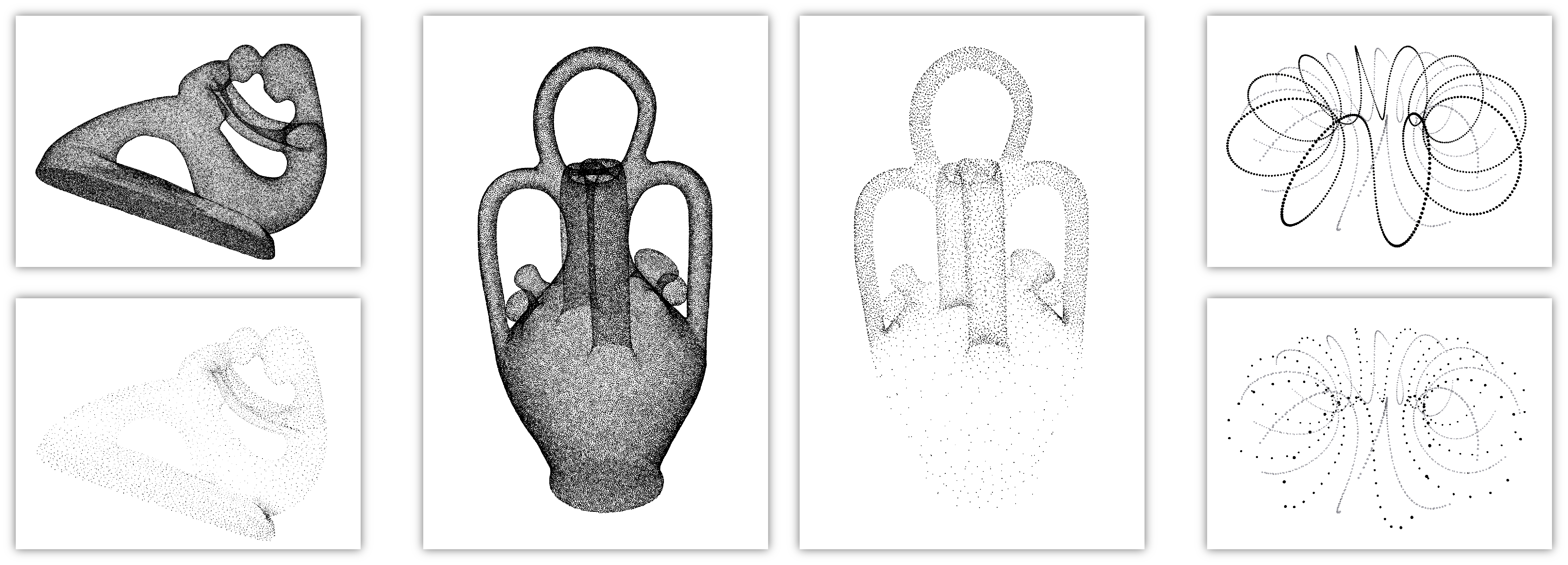
Figure 1: Sparsification: Original samples of 126500 and 101529 points of MotherChild and Botijo are decimated to 6016 and 8622 points respectively. Betti numbers are computed correctly by our algorithm (Section 4). The rightmost picture shows a 3D curve sample (top) and the lean set (bottom) approximating a relevant subset of the medial axis which otherwise spans a much larger subspace of $\mathbb{R}^{3}$.

2 Sparsification

Let ${\mathsf{X}}$ be a smooth compact manifold embedded in a $k$-dimensional ambient Euclidean space $\mathbb{R}^{k}$. Our goal is to sparsify a dense and possibly adaptive sample of ${\mathsf{X}}$ and still be able to recover homological information of ${\mathsf{X}}$ from it.

Distance function, feature size, and sample density.

Let $d(x,A)$ denote the distance between a point $x\in\mathbb{R}^{k}$ and its closest point in a compact set $A\subset\mathbb{R}^{k}$. Consider the distance function $d_{\mathsf{X}}:\mathbb{R}^{k}\to\mathbb{R}$ defined as $d_{\mathsf{X}}(x)=d(x,{\mathsf{X}})$. Let $\Pi(x)=\{y\in{\mathsf{X}}\mid d(x,y)=d(x,{\mathsf{X}})\}$ be the set of closest points of $x\in\mathbb{R}^{k}$ in ${\mathsf{X}}$. Notice that, for any $y\in\Pi(x)$, the segment $xy$ is contained in the normal space $\mathbf{N}_{x}$ of ${\mathsf{X}}$ at $x$. The medial axis $M$ of ${\mathsf{X}}$ is the closure of the set of points with at least two closest points in ${\mathsf{X}}$, and thus $M:={\mathrm{c}losure\,}\{m\in\mathbb{R}^{k}\mid|\Pi(m)|\geq 2\}$.

The local feature size at a point $x\in{\mathsf{X}}$, denoted by ${\mathrm{lfs}}(x)$, is defined as the smallest distance between $x$ and the medial axis $M$; that is, ${\mathrm{lfs}}(x)=d(x,M)$ [2]. There is another feature size definition that is particularly useful for inferring homological information [10]. This feature size is defined as the distance to the critical points of the distance function $d_{\mathsf{X}}$, which is not differentiable everywhere. However, one can still define the following vector which extends the concept of gradient to $d_{\mathsf{X}}$ [18]. Specifically, given any point $x\in\mathbb{R}^{k}\setminus{\mathsf{X}}$, let $c(x)$ be the center of the unique minimal enclosing ball $B_{x}$ enclosing $\Pi(x)$. Define the gradient vector at $x$: $\nabla_{d}(x)=\frac{x-c(x)}{d(x,{\mathsf{X}})}$ and the critical points $C:=\{x\in\mathbb{R}^{k}\,|\,\nabla_{d}(x)=0\}$. The weak local feature size at a point $x\in{\mathsf{X}}$, denoted by ${\mathrm{wlfs}}(x)$, is defined as ${\mathrm{wlfs}}(x)=d(x,C)$. Given an ${\varepsilon}$-dense sample w.r.t. the ${\mathrm{lfs}}$ which is known as the ${\varepsilon}$-sample in the literature [14], we would like to sparsify it to a locally uniform sample w.r.t. some function, ideally ${\mathrm{lfs}}$, or ${\mathrm{wlfs}}$. This motivates the following definition.

Definition 2.1

A discrete sample $P\subset{\mathsf{X}}$ is called $c$-dense w.r.t. a function $\phi:{\mathsf{X}}\rightarrow\mathbb{R}$ if $\forall x\in{\mathsf{X}}$, $d(x,P)\leq c\cdot\phi(x)$. It is $c$-sparse if each pair of distinct points $p,q\in P$ satisfies $d(p,q)\geq c\cdot\phi(p)$. The sample $P$ is called $(c_{1},c_{2})$-uniform w.r.t. $\phi$ if it is $c_{1}$-dense and $c_{2}$-sparse w.r.t. $\phi$.

To produce a $(c_{1},c_{2})$-uniform sample w.r.t. ${\mathrm{lfs}}$ or ${\mathrm{wlfs}}$ one needs to compute ${\mathrm{lfs}}$ or ${\mathrm{wlfs}}$ or their approximations. This in turn needs the computation of at least a subset of the medial axis or its approximation. One option is to approximate this set using the Voronoi poles as in  [2, 3]. This proposition faces two difficulties. First of all, it needs computing the Voronoi diagram in high dimensions. Second, approximating the medial axis may require a large number of samples when a manifold of a low co-dimension is embedded in a high dimensional Euclidean space. To overcome this difficulty we propose to compute a discrete set $L$ near $M$ of small cardinality which helps estimating the distance to a subset of $M$ (See the curve sample in Figure 1 for an example). The set $L$ called the lean set allows us to define an easily computable feature size which we call lean feature size. We show that this feature size is sandwiched between the ${\mathrm{lfs}}$ and ${\mathrm{wlfs}}$ thereby enabling us to sparsify an arbitrarily dense sample to a $(c_{1},c_{2})$-uniform sample w.r.t. a function bracketed by ${\mathrm{lfs}}$ and ${\mathrm{wlfs}}$. The constants $c_{1},c_{2}$ are universal which ultimately leads to a parameter-free inference of the homology.

From now on, we assume that the input $P$ is a dense sample of ${\mathsf{X}}$ in the following adaptive sense [2]. Each point is also equipped with a normal information as stated in Assumption 1. We will see later how this normal information can be computed.

Assumption 2.2

The input point set $P$ is ${\varepsilon}$-dense w.r.t. ${\mathrm{lfs}}$ function on a compact smooth manifold ${\mathsf{X}}\subset\mathbb{R}^{k}$ of known dimension without boundary. Also, every point $p\in P$ has an estimated normal space $\tilde{\mathbf{N}}_{p}$ where $\angle{(\tilde{\mathbf{N}}_{p},\mathbf{N}_{p})}\leq\nu_{\varepsilon}=O({\varepsilon})$ (see Section 2.2 for computations of $\tilde{\mathbf{N}}_{p}$).

Notice that while we assume the input to be ${\varepsilon}$-dense w.r.t. ${\mathrm{lfs}}$, we do not need to know ${\mathrm{lfs}}$ and, locally, the sample can be much denser and non-uniform. Now we define the lean set with respect to which we define the lean feature size.

2.1 Lean set

Definition 2.3

A pair $(p,q)\in P\times P$ is $\beta$-good for $0<\beta<\frac{\pi}{2}$ if the following two conditions hold:

1. $\max\{\angle{(\tilde{\mathbf{N}}_{p},pq)},\angle{(\tilde{\mathbf{N}}_{q},pq)}\}\leq\frac{\pi}{2}-\beta$.

2. Let $v=\frac{p+q}{2}$ be the midpoint of $pq$. The ball $B(v,c_{\beta}d(p,q))$ does not contain any point of $P$ where $c_{\beta}=\frac{1}{3}\tan\frac{\beta}{2}$.

Definition 2.4

The $\beta$-lean set $L_{\beta}$ is defined as:

$$L_{\beta}=\{v|\mbox{ $v=\frac{p+q}{2}$ is the mid point of $pq$ where $(p,q)$ is a $\beta$-good pair\}.}$$

The $\beta$-lean feature size is defined as ${\mathrm{lnfs}_{\beta}}(x)=d(x,L_{\beta})$.

One of our main results is the following property of the lean feature size ( recall the definition of $\nu_{\varepsilon}$ in Assumption 1).

Theorem 2.5

Let $\theta,\beta$ be two positive constants so that $\frac{\pi}{4}\geq\theta\geq\beta+\frac{3}{2}\sqrt{\varepsilon}+\nu_{\varepsilon}$ for a sufficiently small ${\varepsilon}\leq\frac{1}{8}\sin^{2}\theta$. Then,

1. ${\mathrm{lnfs}_{\beta}}(x)\leq c_{1}\cdot{\mathrm{wlfs}}(x)$ for any point $x$ in ${\mathsf{X}}$,

2. ${\mathrm{lnfs}_{\beta}}(p)\geq c_{2}\cdot{\mathrm{lfs}}(p)$ for every point $p\in P$

where $c_{1}=1+\cos\theta+{\varepsilon}$, $c_{2}=\frac{2c_{0}c_{\beta}}{1+c_{0}+2c_{0}c_{\beta}}$, and $c_{0}=\sin(\beta-\nu_{\varepsilon})$, $c_{\beta}=\frac{1}{3}\tan\frac{\beta}{2}$ are positive constants.

The upper bound follows from Proposition 2.7 which shows a stronger result that ${\mathrm{lnfs}_{\beta}}$ is bounded from above by the distance to a subset of the medial axis characterized by an angle condition. This set also contains all critical points of the distance function $d_{\mathsf{X}}$. First, we establish this result.

Definition 2.6

The $\theta$-medial axis $M_{\theta}\subseteq M$ of ${\mathsf{X}}$ is defined as the set of points $m\in M$ where there exist two points $x,y\in\Pi(m)$ such that $\angle{xmy}\geq 2\theta$.

We will see later that the concept of $\theta$-medial axis is also used as a bridge between geometry and topology for our inference result. Our algorithm does not approximate $M_{\theta}$, but rather, approximates the distances to it by the the lean set.

Proposition 2.7

Let $\theta,\beta$ be two positive constants so that $\frac{\pi}{2}\geq\theta\geq\beta+\frac{3}{2}\sqrt{\varepsilon}+\nu_{\varepsilon}$ for a sufficiently small ${\varepsilon}\leq\frac{1}{8}\sin^{2}\theta$. Let $x$ be any point in ${\mathsf{X}}$. Then, ${\mathrm{lnfs}_{\beta}}(x)=d(x,L_{\beta})\leq c\cdot d(x,M_{\theta})$ where $c=1+\cos\theta+{\varepsilon}$ is a positive constant.

Proof.

Let $m=\operatorname{\mathrm{a}rgmin\,}d(x,M_{\theta})$. By definition, we have a pair of points $s,t$ in the manifold ${\mathsf{X}}$ so that the line segments $sm$ and $tm$ subtends an angle larger than or equal to $2\theta$ and both $sm$ and $tm$ are normal to ${\mathsf{X}}$ at $s$ and $t$ respectively. Let $p\in P$ and $q\in P$ be the nearest sample points to $s$ and $t$ respectively. By the ${\varepsilon}$-sampling condition of $P$, we have that $d(p,s)\leq{\varepsilon}{\mathrm{lfs}}(s)$ and thus $\angle{(\mathbf{N}_{s},\mathbf{N}_{p})}\leq{\varepsilon}$.

In Appendix A, we show that the pair $(p,q)$ is $\beta$-good, hence its midpoint $\frac{p+q}{2}$ belongs to $L_{\beta}$. Notice that $\max\{{\mathrm{lfs}}(s),{\mathrm{lfs}}(t)\}\leq d(s,m)=d(t,m)$, and due to the ${\varepsilon}$-sampling condition, $d(\frac{p+q}{2},\frac{s+t}{2})\leq{\varepsilon}d(s,m)$. We then have:

$$d(\frac{p+q}{2},m)\leq d(\frac{s+t}{2},m)+d(\frac{p+q}{2},\frac{s+t}{2})\leq(\cos\theta+{\varepsilon})d(s,m);$$

$$\Rightarrow~{}~{} d(x,L_{\beta})\leq d(x,\frac{p+q}{2})\leq d(x,m)+d(m,\frac{p+q}{2})\leq d(x,m)+d(s,m)(\cos\theta+{\varepsilon}).$$ (1)

Since $s$ is a closest point of $m$ in ${\mathsf{X}}$, we have $d(s,m)=d(m,{\mathsf{X}})\leq d(x,m)$. Combining this with Eqn (1), it follows that

$$d(x,L_{\beta})\leq(1+\cos\theta+{\varepsilon})\cdot d(x,m).$$

∎

We bound the distance $d(x,M_{\theta})$ with ${\mathrm{wlfs}}(x)$ by observing the following. The critical points of a distance function $d:\mathbb{R}^{k}\rightarrow\mathbb{R}$ can be characterized by points $x\in\mathbb{R}^{k}$ that have the zero gradient $\nabla d$ along every unit vector originating at $x$; see Grove [16]. It is also known that the critical points of the distance function $d_{\mathsf{X}}$ lie in the medial axis $M$. They are points $m\in M$ so that the convex hull ${\rm Conv\,}(\Pi(m))$ of all nearest neighbors of $m$ in ${\mathsf{X}}$ contains $m$. This means that there exists a pair of points $x,y$ in $\Pi(m)$ so that the angle $\angle{xmy}$ is large. We use this angle condition to avoid the critical points. Specifically, we show the following result for manifolds of arbitrary codimension which helps to make the angle condition precise.

Proposition 2.8

Let the ambient dimension $k\geq 1$ and $m\in M$ be a critical point of the distance function $d_{\mathsf{X}}$. There exists a pair of points $x,y\in\Pi(m)$ so that $\angle{xmy}\geq\frac{\pi}{2}$.

Proof.

It is known that any critical point $m$ of the distance function $d_{\mathsf{X}}$ is in the convex hull $C={\rm Conv\,}\Pi(m)$ of the points in $\Pi(m)$. This convex hull $C$ is a $j$-polytope for some $j\leq k$. We can assume that $j$ is at least $2$, because otherwise, $C$ is an edge with endpoints say $x,y\in\Pi(m)$, and $\angle{xmy}=\pi\geq\frac{\pi}{2}$.

Now consider the subspace $\mathbb{R}^{j}\subseteq\mathbb{R}^{k}$ that contains the $j$-polytope $C$. Choose an arbitrary $2$-flat $H$ passing through $m$ in this $\mathbb{R}^{j}$. The intersection of $H$ and $C$ is a polygon that contains $m$. There is at least a pair of vertices $u$, $v$ of this polygon so that $\pi\geq\angle{umv}\geq\frac{\pi}{2}$. The vertices $u$ and $v$ are the intersection of the $2$-flat with the two codimension-2 faces $U$ and $V$ of $C$ respectively which are $(j-2)$-faces.

Let $e$ be the maximal line segment contained in $U$ that connects $u$ and a vertex of $U$. We can show that, one can choose an endpoint, say $x$, of $e$ so that the angle $\angle{umv}$ remains at least $\frac{\pi}{2}$ when $u$ assumes the position of $x$. To see this consider the plane $L$ spanned by the line of $e$ and the point $m$ (see figure on the right). Let $t$ be the line perpendicular to the orthogonal projection of $mv$. Observe that all points $z\in e$ makes an angle $\angle{zmv}$ of at least $\frac{\pi}{2}$ if $z$ lies in the halfplane of $L$ delimited by $t$ which does not contain the projection of $mv$. Then, one of the endpoints of $e$ must satisfy this condition because $u\in e$ does so to ensure $\angle{umv}\geq\frac{\pi}{2}$.

The chosen endpoint $x$ of $e$ is either a vertex of $C$ or a point in a lower dimensional face of $U$. Keeping $u$ at $x$, we can let $v$ coincide with a similar endpoint of a line segment in $V$ while keeping the angle $\angle{umv}$ at least $\frac{\pi}{2}$. Therefore, continuing this process, $u$ and $v$ either reach a vertex of $C$ or a lower dimensional face. It follows that both will reach a vertex of $C$ eventually while keeping the angle $\angle{umv}\geq\frac{\pi}{2}$. These two vertices qualify for $x$ and $y$ in the proposition. ∎

Remark 2.9

We remark that the above bound of $\frac{\pi}{2}$ can be further tightened with a term depending on the dimension $k$. However, the bound of $\frac{\pi}{2}$ suffices for our results.

The following assertion is now immediate.

Proposition 2.10

For $\theta\leq\frac{\pi}{4}$, every point $x\in{\mathsf{X}}$ satisfies $d(x,M_{\theta})\leq{\mathrm{wlfs}}(x)$.

Propositions 2.7 and 2.10 together proves the upper bound of the ${\mathrm{lnfs}_{\beta}}$ claimed in Theorem 2.5. Next, we show the lower bound.

Proposition 2.11

For every sample point $p\in P$, we have ${\mathrm{lnfs}_{\beta}}(p)>{c_{2}}\cdot{\mathrm{lfs}}(p)$ where ${c_{2}}=\frac{2c_{0}c_{\beta}}{1+c_{0}+2c_{0}c_{\beta}}$ and $c_{0}=\sin(\beta-\nu_{\varepsilon})$.

Proof.

Let $z$ be the nearest point to $p$ in $L_{\beta}$, and $(p^{\prime},q^{\prime})$ the $\beta$-good pair that gives rise to $z$ (thus $z$ is the midpoint of $p^{\prime}q^{\prime}$). By definition of a $\beta$-good pair, $\angle{(\tilde{\mathbf{N}}_{p^{\prime}},p^{\prime}q^{\prime}))}\leq\frac{\pi}{2}-\beta$ and hence $\angle{(\mathbf{N}_{p^{\prime}},p^{\prime}q^{\prime})}\leq\frac{\pi}{2}-\beta+\nu_{\varepsilon}$. There is a medial ball $B$ tangent to the manifold ${\mathsf{X}}$ at $p^{\prime}$ so that the half line $p^{\prime}o$ going through the center $o$ of this ball $B$ realizes the angle $\angle{(\mathbf{N}_{p^{\prime}},p^{\prime}q^{\prime})}$. Hence, $\angle{op^{\prime}q^{\prime}}\leq\frac{\pi}{2}-\beta+\nu_{\varepsilon}$. It follows that

$$d(p^{\prime},z)=\frac{1}{2}d(p^{\prime},q^{\prime})\geq d(p^{\prime},o)\cos(\frac{\pi}{2}-\beta+\nu_{\varepsilon})\geq c_{0}\cdot{\mathrm{lfs}}(p^{\prime}),\mbox{ where $c_{0}=\sin(\beta-\nu_{\varepsilon})$.}$$ (2)

The empty ball condition of the $\beta$-good pair means that $2c_{\beta}d(p^{\prime},z)\leq d(p,z)$, that is, $d(p^{\prime},z)\leq\frac{d(p,z)}{2c_{\beta}}$. It then follows that

$$d(p,p^{\prime})\leq d(p,z)+d(p^{\prime},z)\leq(1+\frac{1}{2c_{\beta}})d(p,z).$$

By the $1$-Lipschitz property of the ${\mathrm{lfs}}$ function and Eqn (2), we have:

$${\mathrm{lfs}}(p) \leq{\mathrm{lfs}}(p^{\prime})+d(p,p^{\prime})\leq{\mathrm{lfs}}(p^{\prime})+(1+\frac{1}{2c_{\beta}})d(p,z)\leq\frac{1}{c_{0}}d(p^{\prime},z)+(1+\frac{1}{2c_{\beta}})d(p,z)$$

$$\leq\frac{1}{2c_{0}c_{\beta}}d(p,z)+(1+\frac{1}{2c_{\beta}})d(p,z)=(1+\frac{1}{2c_{\beta}}+\frac{1}{2c_{0}c_{\beta}})\cdot d(p,z).$$

Setting ${c_{2}}=\frac{1}{1+\frac{1}{2c_{\beta}}+\frac{1}{2c_{0}c_{\beta}}}=\frac{2c_{0}c_{\beta}}{1+c_{0}+2c_{0}c_{\beta}}$, we have that $d(p,z)={\mathrm{lnfs}_{\beta}}(p)\geq{c_{2}}\cdot{\mathrm{lfs}}(p)$, which proves the proposition. ∎

We will see later that, $\beta$ is fixed at a constant value of $\frac{\pi}{5}$. For this choice of $\beta$, $c_{2}$ is not unusually small.

2.2 Computations for sparsification

In this section we describe the algorithm Lean that takes a standard ${\varepsilon}$-dense sample $P$ w.r.t. ${\mathrm{lfs}}$ of a hidden manifold ${\mathsf{X}}\subset\mathbb{R}^{k}$ of known intrinsic dimension, and outputs a sparsified set $Q\subseteq P$. The set $Q$ is both adaptive and locally uniform as stated afterward in Theorem 2.12. The parameter $\rho$ is chosen later to be a fixed constant less than $1$.

Algorithm 1 Lean($P$, $\beta$, $\rho$)

1:  $L_{\beta}:=\emptyset$;

2:  for every pair $(p,q)\in P\times P$ do

3:     if $(p,q)$ is a $\beta$-good pair then $L_{\beta}:=L_{\beta}\cup\{\frac{p+q}{2}\}$

4:  end for

5:  Put $P$ in a max priority queue ${\mathbb{Q}}$ with priority ${\mathrm{lnfs}_{\beta}}(p)$ for $p\in P$;

6:  while ${\mathbb{Q}}$ not empty  do

7:     $q:=$extract-max(${\mathbb{Q}}$);   $Q:=Q\cup\{q\}$;

8:     delete any $p$ from ${\mathbb{Q}}$ if $d(q,p)\leq\rho{\mathrm{lnfs}_{\beta}}(q)$

9:  end while

The sparsification is based on the lean set $L_{\beta}$, which is computed in lines 2–4 of the algorithm. We note that checking whether a pair $(p,q)$ is $\beta$-good or not requires no parameter other than $\beta$, which is set to a fixed constant $\frac{\pi}{5}$ later in the homology inference algorithm. Clearly, $|L_{\beta}|=O(|P|^{2})$ (see Section 2.3 for improving $|L_{\beta}|$ to $O(|P|)$). There is one implementation detail which involves the estimation of the normal space $\tilde{\mathbf{N}}_{p}$ for every point $p\in P$. This estimation step is oblivious to any parameter but requires the intrinsic dimension $s$ of ${\mathsf{X}}$ to be known.

We estimate the tangent space $T_{p}$ (thus the normal space) of ${\mathsf{X}}$ at a point $p\in P$ as follows. Let $s$ be the intrinsic dimension of the manifold ${\mathsf{X}}$. Let $p_{1}\in P$ be the nearest neighbor of $p$ in $P\setminus\{p\}$. Suppose we have already obtained points $\sigma_{i}=\{p,p_{1},\ldots,p_{i}\}$ with $i<s$. Let ${\mathrm{aff}}(\sigma_{i})$ denote the affine hull of the points in $\sigma_{i}$. Next, we choose $p_{i+1}\in P$ that is closest to $p$ among all points forming an angle within the range $[\frac{\pi}{2}-\frac{\pi}{5},\frac{\pi}{2}]$ with ${\mathrm{aff}}(\sigma_{i})$. We add $p_{i+1}$ to the set and obtain $\sigma_{i+1}=\{p,p_{1},\ldots,p_{i},p_{i+1}\}$. This process is repeated until $i+1=s$, the dimension of ${\mathsf{X}}$, at which point we have obtained $s+1$ points $\sigma_{s}=\{p,p_{1},\ldots,p_{s}\}$. We use ${\mathrm{aff}}(\sigma_{s})$ to approximate the tangent space $T_{p}$. It turns out that the simplex $\sigma_{s}$ obtained this way has good thickness property, which by Corollary 2.6 in [4] implies that the angle between the tangent space and the estimated tangent space at $p$ (thus also the angle between the normal space and the estimated normal space at $p$) is bounded by $O({\varepsilon})$. The big-$O$ hides terms depending only on the intrinsic property of the manifold. See Appendix B for details. In other words, we have that the error $\nu_{\varepsilon}$ in the estimated normal spaces (as required in Assumption 1) is $O({\varepsilon})$.

Next, we put the points in $P$ in a priority queue and process them in the non-decreasing order of their distances to $L_{\beta}$. We iteratively remove the point $q$ with maximum value of $d(q,L_{\beta})$ from the queue and proceed as follows. We put $q$ into the sparse set $Q$ and delete any point from the queue that lies at a distance of at most $\rho{\mathrm{lnfs}_{\beta}}(q)$ from $q$. Since we consider points in non-decreasing order of their distances to $L_{\beta}$, no earlier point that is already in the sparse set $Q$ can be deleted by this process.

Determining if a pair $(p,q)$ is $\beta$-good takes $O(|P|)$ time. This linear complexity is mainly due to the range queries for balls required for testing the ‘empty ball’ condition $2$ for $\beta$-goodness. Therefore, for $L_{\beta}=O(|P|^{2})$, the algorithm spends $O(|P|^{3})$ time in total. This can be slightly improved to $O(|P|^{2-\frac{1}{k}}2^{O(\log^{*}|P|})$ using general spherical range query data structure in the ambient space $\mathbb{R}^{k}$ [1]. Once the lean set is computed, the computation of ${\mathrm{lnfs}}$ for all points involves computing the nearest neighbor in $L_{\beta}$ for each point $p\in P$. Using the method described in section 2.3, we can bring down the lean set size to $O(|P|)$. Then, computing ${\mathrm{lnfs}_{\beta}}$ takes at most $O(|P|^{2})$ time in total. The actual sparsification in steps 6-9 takes only $O(|Q|^{2})=O(|P|^{2})$ time.

We show that the decimation by Lean leaves the point set $Q$ locally uniform w.r.t. ${\mathrm{lnfs}_{\beta}}$. The proof appears in Appendix A.

Theorem 2.12

Let $P$ be a sample of a manifold ${\mathsf{X}}\subseteq\mathbb{R}^{k}$, which is ${\varepsilon}$-dense w.r.t. ${\mathrm{lfs}}$. For $\rho\leq\frac{1}{12}$, the output of ${\sc Lean}(P,\beta,\rho)$ is a $(\frac{4}{3}\rho,\rho)$-uniform sample of ${\mathsf{X}}$ w.r.t. ${\mathrm{lnfs}}_{\beta}$ when ${\varepsilon}>0$ is sufficiently small.

2.3 Linear-size Lean Set

Observe that, the size $|L_{\beta}|$ is $O(n^{2})$ if the input sample $P$ has size $n$. This is far less than $O(n^{\lceil\frac{k}{2}\rceil})$, $k$ being the ambient dimension, which one incurs if the medial axis is approximated with the Voronoi diagrams [9, 14]. We can further thin down the lean set to a linear size $O(n)$ for any fixed $k$ by the following simple strategy:

For every $p\in P$, among all $\beta$-good pairs $(p,q)$ it forms, we choose the pair $(p,q^{*})$ such that the distance $d(p,q^{*})$ is the smallest. We call this pair $(p,q^{*})$ the minimal $\beta$-good pair for $p$. We now take a reduced lean set, denoted by ${\widehat{L}}_{\beta}$, as the collection of midpoints of these minimal $\beta$-good pairs. Obviously, $|{\widehat{L}}_{\beta}|=O(n)$.

Below we show that this reduced lean set can replace the original lean set $L_{\beta}$: it only worsens the distance from a sample point to the lean set by an additional constant factor. Note that this is the only distance in the end required by the algorithm (and the homology inference in Theorem 3.10). In particular, we have the following result.

Lemma 2.13

For any point $p\in P$, we have that ${\mathrm{lnfs}_{\beta}}(p)\leq d(p,{\widehat{L}}_{\beta})\leq(1+\frac{1}{c_{\beta}}){\mathrm{lnfs}_{\beta}}(p).$

Proof.

The left inequality is trivial since ${\widehat{L}}_{\beta}\subseteq L_{\beta}$. We will show the right inequality. Fix any sample point $p\in P$, and let $m\in L_{\beta}$, the midpoint of a $\beta$-good pair $(s,t)$, be $p$’s nearest neighbor in the original lean set $L_{\beta}$.

Let $(s,t^{*})$ be the minimal $\beta$-good pair for $s$, and $m^{*}$ its midpoint. We now show that $d(p,{\widehat{L}}_{\beta})\leq d(p,m^{*})\leq(1+\frac{1}{c_{\beta}})d(p,L_{\beta}).$ Indeed, since $(s,t^{*})$ is the minimal $\beta$-good pair for $s$, we have that $d(s,t)\geq d(s,t^{*})$. Hence

$$d(m,m^{*})\leq d(m,s)+d(s,m^{*})\leq\frac{1}{2}(d(s,t)+d(s,t^{*}))\leq d(s,t).$$

At the same time, by the empty-ball property of a $\beta$-good pair, we have that $d(p,m)\geq c_{\beta}d(s,t)$; that is, $d(s,t)\leq\frac{1}{c_{\beta}}d(p,m)$. Putting everything together, we obtain:

$$d(p,{\widehat{L}}_{\beta})\leq d(p,m^{*})\leq d(p,m)+d(m,m^{*})\leq d(p,m)+d(s,t)\leq(1+\frac{1}{c_{\beta}})d(p,m)=(1+\frac{1}{c_{\beta}})d(p,L_{\beta}).$$

The claim then follows. ∎

3 Homology inference

In this section, we aim to infer homology groups of a hidden manifold ${\mathsf{X}}$ from its point samples. Let ${\sf H}_{i}(\cdot)$ denote the $i$-dimensional homology group. It refers to the singular homology when the argument is a manifold or a compact set, and to the simplicial homology when it is a simplicial complex. All homology groups in this paper are assumed to be defined over the finite field $\mathbb{Z}_{2}$. For details on homology groups, see e.g. [19].

The homology inference from a point sample of a hidden manifold ${\mathsf{X}}$ has been researched extensively in the literature [8, 11, 13, 20]. However, most of these work assume that the given sample $P\subset{\mathsf{X}}$ is globally dense, that is, ${\varepsilon}$-dense w.r.t. to the infimum of ${\mathrm{lfs}}$ or ${\mathrm{wlfs}}$. This strong assumption allows to infer the homology from an appropriate offset of $P$ w.r.t. the distance $d(x,P)$, which is represented with the union of balls of equal radii around the sample points. As we indicated in the introduction, unfortunately, when the sample is adaptive (${\varepsilon}$-dense w.r.t. a non-constant function $\phi$), there may not be such choice of a global radius so that the offset captures the topology of ${\mathsf{X}}$.

To circumvent this problem, one needs to scale the distance with the function $\phi$ that provides the adaptivity. This idea was used in [8] where $\phi$ is taken as ${\mathrm{lfs}}$. Approximating ${\mathrm{lfs}}$ is difficult, so we use ${\mathrm{lnfs}_{\beta}}$ instead for scaling. Observe that the offset may intersect the medial axis, but we argue that we can compute relevant offsets that never contains the critical points of the scaled distance, thereby ensuring topological fidelity.

3.1 Scaled distance and its offsets

In what follows we develop the results in more generality by scaling the distance $d_{\mathsf{X}}$ with the distance to a finite set $L\subset\mathbb{R}^{k}$. Later, in computations, we replace $L$ by the lean set $L_{\frac{\pi}{5}}$ and the distance $d(x,L)$ with ${\mathrm{lnfs}}_{\frac{\pi}{5}}$ for $x\in{\mathsf{X}}$. Recall that $\Pi(x)$ denotes the set of closest neighbors of $x\in\mathbb{R}^{k}$ in ${\mathsf{X}}$.

Definition 3.1

Given a finite set $L\subset\mathbb{R}^{k}$ such that $L\cap{\mathsf{X}}=\emptyset$, Let $h_{L}:\mathbb{R}^{k}\rightarrow\mathbb{R}$ be a scaled distance to the manifold where

$$h_{L}(x)=\frac{d(x,{\mathsf{X}})}{d(x,{\mathsf{X}})+d(x,L)}=\frac{d(x,\Pi(x))}{d(x,\Pi(x))+d(x,L)}.$$

We avoid the obvious choice of $h_{L}(x)=\frac{d(x,{\mathsf{X}})}{d(x,L)}$ because that makes $h_{L}(x)$ unbounded at $L$. We are interested in analyzing the topology of the $\alpha$-offsets ${\mathsf{X}}_{\alpha}=h_{L}^{-1}[0,\alpha]$ of $h_{L}$ (clearly, ${\mathsf{X}}_{0}={\mathsf{X}}$ since $L\cap{\mathsf{X}}=\emptyset$) when ${\mathsf{X}}_{\alpha}\setminus{\mathsf{X}}$ does not include any critical points of $h_{L}$. This brings us to the concept of flow induced by the distance function which was studied in [16] and later used in the context of sampling theory [9, 17, 18]. The vector field $\nabla_{d_{{\mathsf{X}}}}$ as we defined earlier is not continuous. However, as it is shown in [18], there exists a continuous flow ${\mathsf{F}}:\mathbb{R}^{k}\setminus{\mathsf{X}}\times\mathbb{R}^{+}\rightarrow\mathbb{R}^{k}\setminus{\mathsf{X}}$ such that ${\mathsf{F}}(x,t)=x+\int_{0}^{t}\nabla_{d_{{\mathsf{X}}}}({\mathsf{F}}(x,\tau))d\tau$. For a point $x\in\mathbb{R}^{k}\setminus{\mathsf{X}}$, the image ${\mathsf{F}}(x,[0,t])$ of an interval $[0,t]$ is called its flow line. For a point $x\notin{\mathsf{X}}\cup M$, where $M$ is the medial axis of ${\mathsf{X}}$, the flowline ${\mathsf{F}}(x,[0,\infty])$ first coincides with the line segment $x\Pi(x)$ which is normal to the manifold ${\mathsf{X}}$. Once it reaches the medial axis $M$, it stays in $M$. We show that $h_{L}$ increases along the flow line of $d_{\mathsf{X}}$ in the $\alpha$-offset that we are interested in. This, in turn, implies that the $\alpha$-offset of our interest avoids the critical points of $h_{L}$.

Proposition 3.2

For $\theta\leq\frac{\pi}{4}$, $\alpha<\frac{\cos 2\theta}{1+\cos 2\theta}$ and $M_{\theta}\cap{\mathsf{X}}_{\alpha}=\emptyset$, the function $h_{L}$ increases along the flow line on the piece ${\mathsf{X}}_{\alpha}\cap{\mathsf{F}}(x,[0,\infty))$ where $x$ is any point in ${\mathsf{X}}_{\alpha}\setminus{\mathsf{X}}$.

Proof.

First, observe that, due to Proposition 2.8, we can assert that ${\mathsf{X}}_{\alpha}\setminus{\mathsf{X}}$ contains no critical point of $d_{\mathsf{X}}$ since ${\mathsf{X}}_{\alpha}\cap M_{\theta}=\emptyset$ and $\theta\leq\frac{\pi}{4}$. Therefore, flow lines for every point $x\in{\mathsf{X}}_{\alpha}\setminus{\mathsf{X}}$ are (topological) segments. Consider an arbitrary point $y={\mathsf{F}}(x,t)$ such that $y\in{\mathsf{X}}_{\alpha}$. Set $d=d(y,{\mathsf{X}})$ and $\tilde{d}=d(y,L)$. Since $y\in{\mathsf{X}}_{\alpha}$, we have

$$h_{L}(y)\leq\alpha~{}~{}\Longrightarrow~{}~{}\frac{\tilde{d}}{d}\geq\frac{1-\alpha}{\alpha}.$$ (3)

For arbitrary small $\Delta t>0$, let $\Delta d$ and $\Delta\tilde{d}$ denote the changes in the distances $d$ and $\tilde{d}$ respectively when we move on the flow line from $y={\mathsf{F}}(x,t)$ to $y^{\prime}={\mathsf{F}}(x,t+\Delta t)$. Observe that by the triangle inequality, $\Delta\tilde{d}=|d(y,L)-d(y^{\prime},L)|\leq d(y,y^{\prime})$. We claim that $\Delta d\geq d(y,y^{\prime})\cdot\cos 2\phi$ where $\phi$ is the maximum angle so that any point of ${\mathsf{X}}_{\alpha}\cap M$ belongs to $M_{\phi}$.

The flow line ${\mathsf{F}}(x,[0,\infty))$ follows a direction that is normal to the manifold ${\mathsf{X}}$ when it does not lie in the medial axis $M$ of ${\mathsf{X}}$. If $y$ lies on a portion of the flow line which is normal to the manifold ${\mathsf{X}}$, then it is easy to see that $\Delta d=|d(y,{\mathsf{X}})-d(y^{\prime},{\mathsf{X}})|=d(y,y^{\prime})\geq d(y,y^{\prime})\cdot\cos 2\phi$. If $y$ lies on a portion of the flow line which is contained in the medial axis $M$, then the definition of $\phi$ implies that, for any two points $z_{1},z_{2}\in\Pi(y)$, the angle $\angle z_{1}yz_{2}\leq 2\phi$. At the same time, it is known that if $y\in M$, then the flow direction $\nabla_{d_{{\mathsf{X}}}}(y)$ at $y={\mathsf{F}}(x,t)$ points in the direction of $\overrightarrow{oy}$ where $o$ is the center of the minimum enclosing ball for $\Pi(y)$ (see e.g, [18]). In fact, $o$ must be contained in the convex hull of points in $\Pi(y)$. This further leads to that there exists a pair of points $z_{1},z_{2}\in\Pi(y)$ so that the angle between $\overrightarrow{oy}$ and $\overrightarrow{zy}$ for any $z\in\Pi(y)$ is at most the angle $\angle z_{1}yz_{2}$, which is at most $2\phi$. See the figure for an illustration where $\Pi(y)=\{z,z_{1},z_{2},z_{3}\}$, and $T_{z}$ is the intersection of the tangent space of ${\mathsf{X}}$ at $z$ with the plane spanned by $o,y,z$. Hence, in the limit as $y^{\prime}\rightarrow y$, $\Delta d\rightarrow d(y,y^{\prime})\cdot\cos\angle oyz$ for some $z\in\Pi(y)$, implying $\Delta d\geq d(y,y^{\prime})\cdot\cos(2\phi)$.

Finally, note that in the claim, we require that $M_{\theta}\cap{\mathsf{X}}_{\alpha}=\emptyset$. By definition of $\phi$, this means that $\theta>\phi$. Hence, for $\theta\leq\frac{\pi}{4}$, $\frac{\cos 2\theta}{1+\cos 2\theta}=1-\frac{1}{1+\cos 2\theta}\leq 1-\frac{1}{1+\cos 2\phi}$. The condition $\alpha<\frac{\cos 2\theta}{1+\cos 2\theta}$ now provides that $\frac{1}{\cos 2\phi}<\frac{1-\alpha}{\alpha}$. It follows that:

$$\frac{\Delta\tilde{d}}{\Delta d}\leq\frac{1}{\cos 2\phi}<\frac{1-\alpha}{\alpha}\leq\frac{\tilde{d}}{d}\\ \Longrightarrow\frac{\tilde{d}+\Delta\tilde{d}}{d+\Delta d}<\frac{\tilde{d}}{d}\Longrightarrow h_{L}({\mathsf{F}}(x,t))<h_{L}({\mathsf{F}}(x,t+\Delta t)).$$

∎

Now, we will show that the $\alpha$-offset ${\mathsf{X}}_{\alpha}$ remains homotopy equivalent to ${\mathsf{X}}$ if $\alpha$ is chosen appropriately. For the standard distance function $d_{\mathsf{X}}$, such a result is well known [8, 10]. Here, we need the result for the scaled distance $h_{L}$ which we establish using Proposition 3.2 and the critical point theory of Grove [16]. The isotopy lemma of Grove [16] provides the partial result that ${\mathsf{X}}_{\alpha}$ is homotopy equivalent to a smaller offset ${\mathsf{X}}_{\alpha^{\prime}}$, $\alpha^{\prime}<\alpha$. Then we argue that $X_{\alpha^{\prime}}$ is homotopy equivalent to ${\mathsf{X}}$ when $\alpha^{\prime}$ is sufficiently small.

Proposition 3.3

Let $\theta\leq\frac{\pi}{4}$ and $\alpha<\frac{\cos 2\theta}{1+\cos 2\theta}$. Let ${\mathsf{X}}_{\alpha}$ be as defined in proposition 3.2 where ${\mathsf{X}}_{\alpha}\cap M_{\theta}=\emptyset$. Then, ${\mathsf{X}}_{\alpha}$ is homotopy equivalent to ${\mathsf{X}}$ and hence ${\sf H}_{i}({\mathsf{X}}_{\alpha})\cong{\sf H}_{i}({\mathsf{X}})$ for each dimension $i\geq 0$.

Proof.

Consider a real $\alpha^{\prime}$ where $0<\alpha^{\prime}\leq\alpha$. Let $B={\mathrm{C}losure}\,(X_{\alpha}\setminus X_{\alpha}^{\prime})$. Any point $x\in B$ has a flow line ${\mathsf{F}}(x,[0,t])$ along which $h_{L}$ strictly increases (Proposition 3.2). In particular, there is a unit vector originating at $x$ along which $\nabla_{h_{L}}$ does not vanish. Therefore, $B$ does not contain any critical point of $h_{L}$. Applying the isotopy lemma of Grove [16], we conclude that $B$ deformation retracts to the bounding hypersurface $h_{L}^{-1}(\alpha^{\prime})$ of $X_{\alpha}^{\prime}$. The resulting homotopy equivalence can be extended to a map $r:{\mathsf{X}}_{\alpha}=B\cup{\mathsf{X}}_{\alpha^{\prime}}\rightarrow h_{L}^{-1}(\alpha^{\prime})\cup{\mathsf{X}}_{\alpha^{\prime}}={\mathsf{X}}_{\alpha^{\prime}}$ by restricting $r$ to identity on ${\mathsf{X}}_{\alpha^{\prime}}$. It follows that $r$ is a homotopy equivalence.

For any point $x\in{\mathsf{X}}_{\alpha^{\prime}}\setminus{\mathsf{X}}$, a flow line ${\mathsf{F}}(x,[0,t])$ cannot re-enter ${\mathsf{X}}_{\alpha^{\prime}}$ once it exits because of the monotonicity of $h_{L}$. This means ${\mathsf{F}}(x,[0,t])$ intersects ${\mathsf{X}}_{\alpha^{\prime}}$ in one connected segment. Let $x^{\prime}$ be the unique point where ${\mathsf{F}}(x,[0,t])$ intersects the hypersurface $h_{L}^{-1}(\alpha^{\prime})$. Since ${\mathsf{X}}$ is compact and smooth, by choosing $\alpha^{\prime}>0$ sufficiently small, one can ensure that ${\mathsf{F}}(x,[0,t])\cap{\mathsf{X}}_{\alpha^{\prime}}$ lies on the normal line segment $x\Pi(x)$, for all $x\in{\mathsf{X}}_{\alpha^{\prime}}\setminus{\mathsf{X}}$. It implies that ${\mathsf{X}}_{\alpha^{\prime}}$ intersects the normal lines to ${\mathsf{X}}$ in a connected segment along which ${\mathsf{X}}_{\alpha^{\prime}}$ can be retracted to ${\mathsf{X}}$ completing the proof. ∎

3.2 Interleaving and inference

Our goal is to interleave the $\alpha$-offsets of $h_{L}$ with the union of a set of balls $\cup B$ centered at the sample points because then, following the approach in [11], we can relate the topology of the nerve complex of $\cup B$ with that of ${\mathsf{X}}$. For the distance function $d_{\mathsf{X}}$, the offsets restricted to the sample $P$ provide the required set of balls because $d_{{\mathsf{X}}}|_{P}$ approximates $d_{\mathsf{X}}$. Unfortunately, offsets of $h_{L}$ restricted to $P$ are not necessarily union of geometric balls centering points in $P$. Nevertheless, we show that a set of balls whose radii are proportional to the distances to $L$ have the necessary property.

First, we consider the union of balls, one for every point in ${\mathsf{X}}$. Let $\cup B_{\alpha}$ denote the union of balls $B(x,r)$ for every $x\in{\mathsf{X}}$ where $r=\alpha d(x,L)$. One has the following interleaving result.

Proposition 3.4

${\mathsf{X}}_{\frac{\alpha}{1+2\alpha}}\subseteq\cup B_{\alpha}\subseteq{\mathsf{X}}_{\alpha}$.

Proof.

First we show the left inclusion. Let $x$ be any point in ${\mathsf{X}}_{\frac{\alpha}{1+2\alpha}}$, and $y$ an arbitrary point from $\Pi(x)$ (i.e, $d(x,y)=d(x,\Pi(x))$). Then we have,

$$\frac{d(x,y)}{2d(x,y)+d(y,L)} = \frac{d(x,y)}{d(x,y)+(d(x,y)+d(y,L))}$$

$$\leq \frac{d(x,y)}{d(x,y)+d(x,L)}=\frac{\alpha}{1+2\alpha}\mbox{ since $x\in{\mathsf{X}}_{\frac{\alpha}{1+2\alpha}}$}$$

It then follows that

$$(1+2\alpha)d(x,y)\leq 2\alpha d(x,y)+\alpha d(y,L)\Longrightarrow d(x,y)\leq\alpha d(y,L)\Longrightarrow x\in\cup B_{\alpha}.$$

We now prove the second inclusion. Let $x$ be any point in $\cup B_{\alpha}$. Let $z\in{\mathsf{X}}$ be a point so that $x\in B(z,\alpha d(z,L))$; that is, $d(x,z)\leq\alpha d(z,L)$. Such a point exists by the definition of $\cup B_{\alpha}$. Using triangle inequality, we have:

$$h_{L}(x)=\frac{d(x,{\mathsf{X}})}{d(x,{\mathsf{X}})+d(x,L)}\leq\frac{d(x,z)}{d(x,z)+d(x,L)}\leq\frac{d(x,z)}{d(z,L)}\leq\frac{\alpha d(z,L)}{d(z,L)}=\alpha.$$

∎

We extend the above interleaving result to the union of balls whose centers are restricted only to a sample $P\subset{\mathsf{X}}$. For convenience we define the following sampling condition closely related the ${\varepsilon}$-dense sampling condition.

Definition 3.5

A finite set $P\subset{\mathsf{X}}$ is a $(\delta,L)$-sample of ${\mathsf{X}}$ if every point $x\in{\mathsf{X}}$ has a point $p\in P$ so that $d(x,p)\leq\delta d(p,L)$. Furthermore, let $\cup P_{\alpha}=\cup_{p\in P}B(p,\alpha d(p,L))$ denote the union of scaled balls around sample points in $P$.

Remark 3.6

A $\delta$-dense sample w.r.t. ${\mathrm{lnfs}_{\beta}}$ is also a $(\frac{\delta}{1-\delta},L_{\beta})$-sample of ${\mathsf{X}}$. Conversely, a $(\delta,L_{\beta})$-sample of $X$ is also a $\frac{\delta}{1-\delta}$-dense sample w.r.t. ${\mathrm{lnfs}_{\beta}}$. These follow from the fact that ${\mathrm{lnfs}_{\beta}}$ is $1$-Lipschitz.

Proposition 3.7

For a $(\delta,L)$-sample $P$ of ${\mathsf{X}}$ and any $\alpha>0$, we have ${\mathsf{X}}_{\frac{\alpha}{1+2\alpha}}\subseteq\cup P_{\alpha+\delta+\alpha\delta}\subseteq{\mathsf{X}}_{\alpha+\delta+\alpha\delta}.$

Proof.

Recall that by definition $\cup B_{\alpha}=\cup_{x\in{\mathsf{X}}}B(x,\alpha d(x,L))$. By the $(\delta,L)$-sampling condition of $P$, as well as triangle inequality, we have $\cup B_{\alpha}\subseteq\cup P_{\alpha+\delta+\alpha\delta}$. Combining this with the left inclusion in Proposition  3.4, we have

$${\mathsf{X}}_{\frac{\alpha}{1+2\alpha}}\subseteq\cup B_{\alpha}\subseteq\cup P_{\alpha+\delta+\alpha\delta}.$$

The second inclusion follows because $\cup P_{\alpha+\delta+\alpha\delta}\subseteq\cup B_{\alpha+\delta+\alpha\delta}$ and $\cup B_{\alpha+\delta+\alpha\delta}\subseteq{\mathsf{X}}_{\alpha+\delta+\alpha\delta}$ (Proposition 3.4). ∎

With the isomorphisms in the homology groups of the offset of our scaled distance function (Proposition 3.3) and the interleaving result (Proposition 3.7), we can infer the homology of the hidden manifold ${\mathsf{X}}$ from the union of balls $\cup P_{\alpha}$.

Suppose that $P$ is a $(\delta,L)$-sample of the manifold ${\mathsf{X}}$. Recall that $\cup P_{\alpha}$ denotes the union of balls $\bigcup_{p\in P}B(p,\alpha d(p,L))$ centered at each point $p\in P$, with radius $\alpha d(p,L)$. Note that the parameter $\alpha$ does not stand for distance threshold, but a scale parameter for the distance $d(p,L)$. This parameter is universal for all points, while the distance $d(p,L)$ makes the union of balls adaptive.

By manipulating the result in Proposition  3.7, one obtains that, for $\alpha+\delta\leq\frac{1}{4}$ and $\alpha^{\prime}=\frac{\alpha}{2(1-\alpha)}$,

$${\mathsf{X}}_{\frac{\alpha}{2}}\subseteq\cup P_{\alpha^{\prime}+\delta+\alpha^{\prime}\delta}\subseteq\cup P_{\frac{5}{4}\alpha^{\prime}+\delta}\subseteq\cup P_{\alpha+\delta}$$

When $\alpha+\delta\leq\frac{1}{6}$ and $\alpha^{\prime}=\frac{\alpha+\delta}{1-2(\alpha+\delta)}$, similar manipulation gives

$${\mathsf{X}}_{\alpha+\delta}\subseteq\cup P_{\alpha^{\prime}+\delta+\alpha^{\prime}\delta}\subseteq\cup P_{\frac{7}{6}\alpha^{\prime}+\delta}\subseteq\cup P_{\frac{11}{4}(\alpha+\delta)}\subseteq\cup P_{3(\alpha+\delta)}$$

So, for $\alpha+\delta\leq\frac{1}{6}$, we obtain

$${\mathsf{X}}_{\frac{\alpha}{2}}\subseteq\cup P_{\alpha+\delta}\subseteq{\mathsf{X}}_{\alpha+\delta}\subseteq\cup P_{3(\alpha+\delta)}\subseteq{\mathsf{X}}_{3(\alpha+\delta)}$$ (4)

which leads to inclusion-induced homomorphisms at the homology level that interleave:

$${\sf H}_{i}({\mathsf{X}}_{\frac{\alpha}{2}})\rightarrow{\sf H}_{i}(\cup P_{\alpha+\delta})\rightarrow{\sf H}_{i}({\mathsf{X}}_{\alpha+\delta})\rightarrow{\sf H}_{i}(\cup P_{3(\alpha+\delta)})\rightarrow{\sf H}_{i}({\mathsf{X}}_{3(\alpha+\delta)})$$

On the other hand, if $3(\alpha+\delta)<\frac{\cos 2\theta}{1+\cos 2\theta}$ and ${\mathsf{X}}_{3(\alpha+\delta)}\cap M_{\theta}=\emptyset$, we can use Proposition 3.3 and Lemma 3.2 in [11] to claim that

$${\mathrm{image}\,}({\sf H}_{i}(\cup P_{\alpha+\delta})\rightarrow{\sf H}_{i}(\cup P_{3(\alpha+\delta)}))\cong{\sf H}_{i}({\mathsf{X}}).$$

Let $C^{\alpha}(P)$ denote the nerve of $\cup P_{\alpha}$. One can recognize the resemblance between $C^{\alpha}(P)$ and the well-known Čech complex. Both are nerves of unions of closed balls, but unlike Čech complexes, $C^{\alpha}(P)$ is the nerve of a union of balls that may have different radii; recall that $\alpha$ denotes a fraction relative to a distance rather than an absolute distance. The Nerve Lemma [5] provides that $C^{\alpha}(P)$ is homotopy equivalent to $\cup P_{\alpha}$. Also, the argument of Chazal and Oudot [11] to prove Theorem 3.5 can be extended to claim that for any $i\geq 0$,

$${\mathrm{rank}}\,({\sf H}_{i}(C^{\alpha+\delta}(P))\rightarrow{\sf H}_{i}(C^{3(\alpha+\delta)}(P))={\mathrm{rank}}\,({\sf H}_{i}(\cup P_{\alpha+\delta})\rightarrow{\sf H}_{i}(\cup P_{3(\alpha+\delta)}))={\mathrm{rank}}\,{\sf H}_{i}({\mathsf{X}}).$$

The complex $C^{\alpha}(P)$ interleaves with another complex $R^{\alpha}(P)$ that is reminiscent of the interleaving of the Čech with the Vietoris-Rips complexes. Specifically, let

$$R^{\alpha}(P):=\{\sigma\,|\,d(p,q)\leq\alpha(d(p,L)+d(q,L))\mbox{ for every edge $pq$ of $\sigma$}\}.$$

It is easy to observe that $R^{\alpha}(P)$ is the completion of the $1$-skeleton of $C^{\alpha}(P)$ and the following inclusions hold as in the case of the original Čech and Vietoris-Rips complexes.

$$C^{\alpha}(P)\subseteq R^{\alpha}(P)\subseteq C^{2\alpha}(P)\mbox{ for any $\alpha\geq 0$}.$$

Now, by choosing $\alpha+\delta\leq\frac{1}{6}\frac{\cos 2\theta}{1+\cos 2\theta}$ (which also implies $\alpha+\delta\leq\frac{1}{12}$ since $\frac{\cos 2\theta}{1+\cos 2\theta}\leq\frac{1}{2}$), we have a sequence similar to (4) that eventually induces the following sequence:

$${\sf H}_{i}(C^{\alpha+\delta}(P))\rightarrow{\sf H}_{i}(R^{\alpha+\delta}(P))\rightarrow{\sf H}_{i}(C^{2(\alpha+\delta)}(P))\rightarrow{\sf H}_{i}(C^{6(\alpha+\delta)}(P))\rightarrow{\sf H}_{i}(R^{6(\alpha+\delta)}(P))\rightarrow{\sf H}_{i}(C^{12(\alpha+\delta)}(P)).$$

In particular, following a similar argument as before, we have that

$${\mathrm{rank}}\,({\sf H}_{i}(C^{\alpha+\delta}(P))\rightarrow{\sf H}_{i}(C^{12(\alpha+\delta)}(P))={\mathrm{rank}}\,({\sf H}_{i}(C^{2(\alpha+\delta)}(P))\rightarrow{\sf H}_{i}(C^{6(\alpha+\delta)}(P))={\mathrm{rank}}\,{\sf H}_{i}({\mathsf{X}})$$

as long as $12(\alpha+\delta)\leq\frac{\cos 2\theta}{1+\cos 2\theta}$ and ${\mathsf{X}}_{12(\alpha+\delta)}\cap M_{\theta}=\emptyset$. By using the standard results of interleaving [11] on this sequence, we obtain that

$${\mathrm{rank}}({\sf H}_{i}(R^{\alpha+\delta}(P))\rightarrow{\sf H}_{i}(R^{6(\alpha+\delta)}(P)))={\mathrm{rank}}\,{\sf H}_{i}({\mathsf{X}}).$$

Theorem 3.8

For a finite set $L\subset\mathbb{R}^{k}$ where $L\cap{\mathsf{X}}=\emptyset$, let $P$ be a $(\delta,L)$-sample of the manifold ${\mathsf{X}}\subset\mathbb{R}^{k}$. Let $\theta\leq\frac{\pi}{4}$, and $\alpha+\delta\leq\frac{1}{12}\frac{\cos 2\theta}{1+\cos 2\theta}$. If ${\mathsf{X}}_{12(\alpha+\delta)}\cap M_{\theta}=\emptyset$, then $\mathrm{rank}({\sf H}_{i}({\mathsf{X}}))=\mathrm{rank}({\sf H}_{i}(R^{\alpha+\delta}(P))\rightarrow{\sf H}_{i}(R^{6(\alpha+\delta)}(P)))$, for any $i\geq 0$.

3.3 Computations for topology inference

Algorithm 2 LeanTopo($P$)

1:  $\beta:=\frac{\pi}{5}$;   $\rho:=\frac{1}{26}\frac{\cos 2\beta}{1+\cos 2\beta}$;   $Q:={{\sc Lean}}(P,\beta,\rho)$;

2:  Compute the complexes $R^{2\rho}(Q)$ and $R^{12\rho}(Q)$;

3:  Compute the persistence induced by the inclusion $R^{2\rho}(Q)\rightarrow R^{12\rho}(Q)$.

In step 3 of LeanTopo, we compute the persistence homology induced by the inclusion $R^{2\rho}(Q)\rightarrow R^{12\rho}(Q)$ where $\rho=\frac{1}{26}\frac{\cos 2\beta}{1+\cos 2\beta}$. When the parameter ${\varepsilon}$ is sufficiently small and $\beta=\frac{\pi}{5}$, we can find a value $\theta$ such that $\frac{\pi}{4}\geq\theta\geq\beta+\frac{3}{2}\sqrt{{\varepsilon}}+\nu_{\varepsilon}$ and $2\rho=\frac{1}{13}\frac{\cos 2\beta}{1+\cos 2\beta}\leq\frac{1}{12}\frac{\cos 2\theta}{1+\cos 2\theta}$. This is precisely what is needed for the homology inference in Theorem 3.8. More specifically, recall by Eqn. 7 in the proof of Theorem 2.12, the output sparsified set of points $Q$ is a $(\delta,L_{\frac{\pi}{5}})$-sample for $\delta=\frac{6}{5}\rho$. The algorithm implicitly sets $\alpha=2\rho-\delta=\frac{4}{5}\rho$ such that $\alpha+\delta=2\rho\leq\frac{1}{12}\frac{\cos 2\theta}{1+\cos 2\theta}$ when ${\varepsilon}$ is sufficiently small. Theorem 3.8 requires further that the offset ${\mathsf{X}}_{\alpha^{\prime}}:=h^{-1}_{L_{\frac{\pi}{5}}}[0,\alpha^{\prime}]$ is disjoint from $M_{\theta}$ for $\alpha^{\prime}=12(\alpha+\delta)$ which we establish using the following proposition.

Proposition 3.9

Let $\alpha^{\prime}\leq\frac{1}{1+\cos\theta+{\varepsilon}}$ and $\theta$ be such that $\frac{\pi}{2}\geq\theta\geq\frac{\pi}{5}+\frac{3}{2}\sqrt{\varepsilon}+\nu_{\varepsilon}$ for a sufficiently small ${\varepsilon}\leq\frac{1}{8}\sin^{2}\theta$. Then, $M_{\theta}\cap{\mathsf{X}}_{\alpha^{\prime}}=\emptyset.$

Proof.

We prove the result by contradiction. Assume that there exists a point $x\in M_{\theta}\cap{\mathsf{X}}_{\alpha^{\prime}}$. Define $m$ and $s$ as in the proof of Proposition 2.7. With $\beta=\frac{\pi}{5}$, the assumed conditions for $\theta,\beta,{\varepsilon}$ are same as in Proposition 2.7, and thus we can arrive at the inequality 1 in its proof. Since $s$ is a closest point of $m$ in ${\mathsf{X}}$, we have $d(s,m)=d(m,{\mathsf{X}})\leq d(x,m)+d(x,{\mathsf{X}})$. Combining this with Eqn (1), it follows that, for any $x\in{\mathsf{X}}_{\alpha^{\prime}}$,

$$d(x,L_{\frac{\pi}{5}})\leq(1+\cos\theta+{\varepsilon})\cdot d(x,m)+(\cos\theta+{\varepsilon})\cdot d(x,{\mathsf{X}}).$$

Since $x\in{\mathsf{X}}_{\alpha^{\prime}}$, $h_{L_{\frac{\pi}{5}}}(x)\leq\alpha^{\prime}$ implies that $d(x,{\mathsf{X}})\leq\frac{\alpha^{\prime}}{1-\alpha^{\prime}}d(x,L_{\frac{\pi}{5}})$. Hence $d(x,L_{\frac{\pi}{5}})\leq c\cdot d(x,m)=c\cdot d(x,M_{\theta})$ for the positive constant $c=\frac{1+\cos\theta+{\varepsilon}}{1-\frac{\alpha^{\prime}}{1-\alpha^{\prime}}(\cos\theta+{\varepsilon})}=1+\frac{\cos\theta+{\varepsilon}}{1-\alpha^{\prime}(1+\cos\theta+{\varepsilon})}$.

On the other hand, since $x\in M_{\theta}\cap{\mathsf{X}}_{\alpha^{\prime}}$ and since ${\mathsf{X}}\cap M_{\theta}$ is empty, $x\not\in{\mathsf{X}}$. Thus, $d(x,{\mathsf{X}})>0$. Since $x\in{\mathsf{X}}_{\alpha^{\prime}}$ and $h_{L_{\frac{\pi}{5}}}(x)\leq\alpha^{\prime}$, we have that $d(x,L_{\frac{\pi}{5}})\geq\frac{1-\alpha^{\prime}}{\alpha^{\prime}}d(x,{\mathsf{X}})$. Hence $d(x,L_{\frac{\pi}{5}})>0$ as well since $\alpha^{\prime}<1$. This further implies that $d(x,M_{\theta})>0$ because according to the above derivation, $d(x,M_{\theta})\geq\frac{1}{c}d(x,L_{\frac{\pi}{5}})$ for $c>0$. This however contradicts the fact that $x\in M_{\theta}\cap{\mathsf{X}}_{\alpha^{\prime}}\in M_{\theta}$. Hence our assumption is wrong and there is no such point $x\in M_{\theta}\cap{\mathsf{X}}_{\alpha^{\prime}}$. ∎

Theorem 3.10

Let ${\mathsf{X}}\subset\mathbb{R}^{k}$ be a smooth compact manifold without boundary of known intrinsic dimension. Let $P$ be an ${\varepsilon}$-dense sample of ${\mathsf{X}}$ w.r.t. ${\mathrm{lfs}}$. LeanTopo$(P)$ computes the rank of ${\sf H}_{i}({\mathsf{X}})$ for any $i\geq 0$ when ${\varepsilon}$ is sufficiently small.

Proof.

Since $\frac{\cos 2\theta}{1+\cos 2\theta}\leq\frac{1}{1+\cos\theta+{\varepsilon}}$ for $\theta\leq\frac{\pi}{2}$ and small enough ${\varepsilon}$, one has the fact that $\alpha^{\prime}=12(\alpha+\delta)\leq\frac{\cos 2\theta}{1+\cos 2\theta}$ implies that $\alpha^{\prime}\leq\frac{1}{1+\cos\theta+{\varepsilon}}$. This means that the parameters $\alpha,$ and $\theta$ set by the algorithm LeanTopo implicitly or explicitly satisfy the conditions required by Proposition 3.9. Hence, ${\mathsf{X}}_{12(\alpha+\delta)}\cap M_{\theta}=\emptyset$. Therefore, all conditions for Theorem 3.8 hold for the sparsified set $Q$ output by Lean, and it then follows that $\mathrm{rank}({\sf H}_{i}({\mathsf{X}}))=\mathrm{rank}({\sf H}_{i}(R^{2\rho}(Q))\to{\sf H}_{i}(R^{12\rho}(Q)))$, for any $i\geq 0$. ∎

We remark that a particular interesting feature of Algorithm LeanTopo is that, we only need to set the parameter $\beta$ to a universal constant $\frac{\pi}{5}$. All other parameters such as the angle and radius conditions for choosing $\beta$-good pairs and the decimation radius are determined by this choice of the angle $\beta$. This makes LeanTopo parameter-free; see also our experimental results in Section 4. At the same time, the above Theorem states that its output is guaranteed to be correct as the input set of samples $P$ becomes sufficiently dense.

4 Experiments and discussion

We experimented with LeanTopo primarily on curve and surface samples. We used thresholds for sparsification that are more aggressive than predicted by our analysis. For example, our analysis predicts that for $\beta=\frac{\pi}{5}$, the constant $c_{\beta}=\frac{1}{3}\tan\frac{\beta}{2}\approx 0.11$, but we kept it at $0.5$. We kept the same thresholds for all models to ensure that we don’t fine tune it for different input. The decimation ratio $\frac{r_{q}}{d(q,L_{\beta})}$ is kept at $0.5$, and the $r$ for computing the complex $R^{r}$ is kept at $0.65$ in all cases. Table 1 below shows the details. The rank of $H_{1}$ homology is computed correctly by our algorithm for all these data. The sparsified points are shown in Figure 1.

Name	input #points	output #points	$c_{\beta}$	decimation ratio	$r$ for $R^{r}$	${\mathrm{r}ank}\,H_{1}$
MotherChild	126500	5267	0.5	0.5	0.7	8
Botijo	101529	7600	0.5	0.5	0.7	10
Kitten	134448	1914	0.5	0.5	0.7	2
CurveHelix	1000	235	0.5	0.5	0.7	1

Table 1: Experiments on a curve and three surface samples.

Extensions.

One obvious question that remains open is how to extend the scope of our sparsification strategy to larger class of input, such as noisy data samples and/or samples from compact spaces rather than manifolds.

Noise: We observe that, for Hausdorff noise, where samples are assumed to lie within a small offset of the manifold, our method can be applied. However, a parameter giving the extent of this Hausdorff noise needs to be supplied. With this parameter, one can estimate the normals reliably from the noisy but dense sample. The step where we compute the lean set, requires an empty ball test which also needs this parameter because otherwise noise can collaborate to provide a false impression that some spurious manifolds have been sampled. Given the ambiguity that a noisy sample can be dense for two topologically different spaces, it may be impossible to avoid a parameter that eliminates different such possibilities. Nevertheless, our method would free the user from specifying a threshold for building the complexes.

In an experiment, we added artificial noise on the three surface samples as shown in Figure 2 to test robustness of our algorithm. We added a uniform displacement to each sample point along the normal direction. The displacement ranged from $-0.5\%$ to $0.5\%$ times the diameter of the model. We modified our algorithm to ignore all leanset points formed by two points closer than a threshold which is picked as a multiple of the diameter of the model. Other thresholds were kept the same as in the previous experiment. Results in Table 2 show that the algorithm can tolerate noise in case there is a known upper limit on the noise level.

Threshold (multiple of noise scale)	0	1	2	3	4	5	6	7	8	9	10	11	12	13
MotherChild	18196	1636	37	8	8	8	8	8	8	8	8	8	7	7
Botijo	14565	14580	1462	10	10	10	10	10	10	10	10	8	8	8
Kitten	20506	20572	1314	2	2	2	2	2	2	2	2	2	2	2

Table 2: Experiments on 3 surfaces with artificial noise. The table shows resulting $H_{1}$ of each model under different threshold. Experiments show that the influence of noise is removed when we pick threshold greater than or equal to 3 times of the noise scale. The threshold might introduce problem when it is too large.

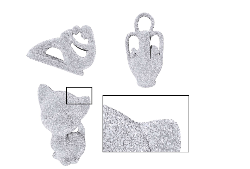
Figure 2: Noisy samples. Meshes are created only for rendering.

The more general noise model which allows outliers would also be worthwhile to investigate. One may explore the ‘distance to measure’ technique proposed in [7] for this case. But, it is not clear how to adapt the entire development in this paper to this setting. One possibility is to eliminate all outliers first to make the noise only Hausdorff, and then apply the technique for Hausdorff noise as alluded in the previous paragraph. This will certainly require more parameters to be supplied by the user.

Compacts: The case for compact sets is perhaps more challenging. The normal spaces are not well defined everywhere for such spaces. Thus, we need to devise a different strategy to compute the lean set. The theory of compacts developed in the context of topology inference in [6] may be useful here. Computing the lean sets efficiently in high dimensions for compact spaces remain a formidable open problem.

Appendix A Missing Proofs

Proving that $(p,q)$ is $\beta$-good for Proposition 2.7.

We know that $\angle{(\mathbf{N}_{s},st)}\leq\pi/2-\theta$ which implies that $d(s,t)\geq 2d(s,m)\sin\theta\geq 2{\mathrm{lfs}}(s)\sin\theta$. Consider the triangle $pst$. By triangle inequality, $d(p,t)\geq d(s,t)-d(s,p)\geq(2\sin\theta-{\varepsilon}){\mathrm{lfs}}(s)$. The angle $\angle{pts}$ is at most

$$\arcsin\frac{d(p,s)}{d(p,t)}\leq\arcsin\frac{{\varepsilon}{\mathrm{lfs}}(s)}{(2\sin\theta-{\varepsilon}){\mathrm{lfs}}(s)}\leq\frac{4}{3}\cdot\frac{{\varepsilon}}{2\sin\theta-{\varepsilon}}.$$ (5)

The last inequality follows from that $\arcsin(x)\leq cx$ for $x\leq\frac{\sqrt{c^{2}-1}}{c}$. In our case, choose $c=\frac{4}{3}$. Since $\sqrt{{\varepsilon}}\leq\frac{\sin\theta}{2\sqrt{2}}\leq\frac{1}{2}$, we have that

$$\frac{{\varepsilon}}{2\sin\theta-{\varepsilon}}\leq\frac{{\varepsilon}}{4\sqrt{{\varepsilon}}-{\varepsilon}}=\frac{\sqrt{{\varepsilon}}}{4-\sqrt{{\varepsilon}}}\leq\frac{1}{7}\leq\frac{\sqrt{c^{2}-1}}{c}.$$

Now assume without loss of generality that ${\mathrm{lfs}}(s)\geq{\mathrm{lfs}}(t)$. Then,

$$d(p,q)\geq d(s,t)-d(p,s)-d(q,t)\geq d(s,t)-2{\varepsilon}{\mathrm{lfs}}(s)\geq 2(\sin\theta-{\varepsilon}){\mathrm{lfs}}(s).$$

Recall that $d(t,p)\geq(2\sin\theta-{\varepsilon}){\mathrm{lfs}}(s)$. Considering the triangle $tpq$, we have

$$\angle{tpq}\leq\arcsin\frac{d(q,t)}{d(p,t)}\leq\arcsin\frac{{\varepsilon}{\mathrm{lfs}}(t)}{2(\sin\theta-{\varepsilon}){\mathrm{lfs}}(s)}\leq\arcsin\frac{{\varepsilon}{\mathrm{lfs}}(s)}{2(\sin\theta-{\varepsilon}){\mathrm{lfs}}(s)}\leq\frac{4}{3}\cdot\frac{{\varepsilon}}{2(\sin\theta-{\varepsilon})},$$ (6)

where the last inequality follows from a similar argument used for Eqn. (5).

We know that, $\angle{(\mathbf{N}_{p},\mathbf{N}_{s})}\leq{\varepsilon}$, $\angle{(\tilde{\mathbf{N}}_{p},\mathbf{N}_{p})}\leq\nu_{{\varepsilon}},$ and $\angle{(pq,st)}\leq\angle pts+\angle tpq$. Combining these with Eqn. (5), (6) and the assumption that $\sqrt{{\varepsilon}}\leq\frac{1}{2\sqrt{2}}\sin\theta(\leq\frac{1}{2})$, we have that

$$\angle{(pq,\tilde{\mathbf{N}}_{p})} \leq\angle{(pq,st)}+\angle{(st,\mathbf{N}_{s})}+\angle{(\mathbf{N}_{s},\mathbf{N}_{p})}+\angle{(\mathbf{N}_{p},\tilde{\mathbf{N}}_{p})}\leq\frac{8}{3}\cdot\frac{{\varepsilon}}{2\sin\theta-2{\varepsilon}}+\frac{\pi}{2}-\theta+{\varepsilon}+\nu_{\varepsilon}$$

$$\leq\frac{8}{3}\cdot\frac{\sqrt{{\varepsilon}}}{4\sqrt{2}-2\sqrt{{\varepsilon}}}+\frac{\sqrt{{\varepsilon}}}{2}+\frac{\pi}{2}-\theta+\nu_{\varepsilon}\leq\frac{\pi}{2}-\theta+\frac{3}{2}\sqrt{{\varepsilon}}+\nu_{\varepsilon}$$

Similar bound holds for $\angle{(pq,\tilde{\mathbf{N}}_{q})}$. It follows that the pair $(p,q)$ satisfies the first condition of being $\beta$-good, as long as $\frac{\pi}{2}-\theta+\frac{3}{2}\sqrt{{\varepsilon}}+\nu_{\varepsilon}\leq\frac{\pi}{2}-\beta$. This is guaranteed by requiring $\theta\geq\beta+\frac{3}{2}\sqrt{\varepsilon}+\nu_{\varepsilon}$ (as specified in the proposition).

Next, we argue that $(p,q)$ also satisfies the second condition of being $\beta$-good. To do so, let ${\tilde{\theta}}=\frac{1}{2}\angle smt$ be half of the angle spanned by $sm$ and $tm$. Note that by the definition of $\theta$-medial axis $M_{\theta}$, we have that ${\tilde{\theta}}\geq\theta$. See the right figure for an illustration. First, observe that the ball $D=B(\frac{s+t}{2},r)$ with $r=d(s,m)\cdot(1-\cos{\tilde{\theta}})$ does not intersect ${\mathsf{X}}$, since this ball is contained inside the medial ball $B(m,d(s,m))$. The midpoint $\frac{p+q}{2}$ of $pq$ is at most ${\varepsilon}{\mathrm{lfs}}(s)\leq{\varepsilon}d(s,m)$ distance away from $\frac{s+t}{2}$ because both $p$ and $q$ are at most ${\varepsilon}{\mathrm{lfs}}(s)$ away from $s$ and $t$ (assuming w.o.l.g ${\mathrm{lfs}}(s)\geq{\mathrm{lfs}}(t)$). This means that the ball $D^{\prime}=B(\frac{p+q}{2},r^{\prime})$ centering at the midpoint of $pq$ and with radius $r^{\prime}=d(s,m)\cdot(1-\cos{\tilde{\theta}}-{\varepsilon})$ is contained in the ball $D$ and thus does not have any point of ${\mathsf{X}}$ and hence $P$ inside.

On the other hand, note that

$$d(p,q)\leq d(s,t)+2{\varepsilon}{\mathrm{lfs}}(s)\leq 2d(s,m)\sin{\tilde{\theta}}+2{\varepsilon}d(s,m)=2d(s,m)(\sin{\tilde{\theta}}+{\varepsilon}).$$

Thus, the second condition for $p,q$ being a good pair is satisfied as long as

$$c_{\beta}\leq\frac{1-\cos{\tilde{\theta}}-{\varepsilon}}{2(\sin{\tilde{\theta}}+{\varepsilon})}\leq\frac{r^{\prime}}{d(p,q)}.$$

Consider the function $f(x)=\frac{1-\cos x-{\varepsilon}}{\sin x+{\varepsilon}}$, its derivative $f^{\prime}(x)$ is greater than $0$ for $x\in[0,\pi/2]$. Indeed,

$$f^{\prime}(x)=\frac{\sin x\cdot(\sin x+{\varepsilon})-(1-\cos x-{\varepsilon})\cdot\cos x}{(\sin x+{\varepsilon})^{2}}=\frac{1-\cos x+{\varepsilon}\sin x+{\varepsilon}\cos x}{(\sin x+{\varepsilon})^{2}}\geq 0.$$

Hence $f(x)$ is an increasing function, and $f({\tilde{\theta}})\geq f(\theta)$ since ${\tilde{\theta}}\geq\theta$. In other words, the second condition for $(p,q)$ being a good pair is satisfied as long as $c_{\beta}\leq\frac{1-\cos\theta-{\varepsilon}}{2(\sin\theta+{\varepsilon})}$. To further simplify it, note that using ${\varepsilon}\leq\frac{1}{8}\sin^{2}\theta$, one can show that $\frac{4{\varepsilon}}{\sin\theta}\leq\tan\frac{\theta}{2}$. Combining this with $\frac{1-\cos\theta}{\sin\theta}=\tan\frac{\theta}{2}$, we then have

$$\frac{1-\cos\theta-{\varepsilon}}{2(\sin\theta+{\varepsilon})}\geq\frac{1-\cos\theta-{\varepsilon}}{\frac{9}{4}\sin\theta}=\frac{4}{9}\tan\frac{\theta}{2}-\frac{4{\varepsilon}}{9\sin\theta}\geq\frac{4}{9}\tan\frac{\theta}{2}-\frac{1}{9}\tan\frac{\theta}{2}=\frac{1}{3}\tan\frac{\theta}{2}\geq\frac{1}{3}\tan\frac{\beta}{2}.$$

Hence as $c_{\beta}\leq\frac{1}{3}\tan\frac{\beta}{2}$, the ball $B(\frac{p+q}{2},c_{\beta}d(p,q))$ is contained in $D^{\prime}$ and thus contains no point in $P$. Therefore, the pair $(p,q)$ is $\beta$-good and its midpoint is in $L_{\beta}$.

Proof of Theorem 2.12.

Let $x$ be any point in ${\mathsf{X}}$ to which $p$ is the nearest sample point in $P$. Then, $d(x,p)\leq{\varepsilon}{\mathrm{lfs}}(x)\leq{\varepsilon}^{\prime}{\mathrm{lfs}}(p)$ where ${\varepsilon}^{\prime}=\frac{{\varepsilon}}{1-{\varepsilon}}$. If $p$ is retained in $Q$, $d(x,Q)\leq{\varepsilon}{\mathrm{lfs}}(x)\leq{\varepsilon}^{\prime}{\mathrm{lfs}}(p)\leq\frac{{\varepsilon}^{\prime}}{{c_{2}}}d(p,L_{\beta})\leq\frac{6\rho}{5}d(p,L_{\beta})$ for sufficiently small ${\varepsilon}>0$, where ${c_{2}}$ is the constant from Proposition 2.11. Now consider the case when $p$ is deleted while processing another point, say $q\in P$. By the decimation procedure in lines 5–9, $d(q,L_{\beta})\geq d(p,L_{\beta})$ and $q$ will remain in $Q$ since we process points in non-decreasing order of their distances to $L_{\beta}$. Using Proposition 2.11, we then have:

$$d(x,q) \leq d(x,p)+d(p,q)\leq{\varepsilon}{\mathrm{lfs}}(x)+\rho d(q,L_{\beta})\leq{\varepsilon}^{\prime}{\mathrm{lfs}}(p)+\rho d(q,L_{\beta})$$

$$\leq\frac{{\varepsilon}^{\prime}}{{c_{2}}}d(p,L_{\beta})+\rho d(q,L_{\beta})\leq(\frac{{\varepsilon}^{\prime}}{{c_{2}}}+\rho)d(q,L_{\beta})\leq\frac{6\rho}{5}d(q,L_{\beta}).$$

The last inequality holds when ${\varepsilon}$ is sufficiently small (in which case the estimation error $\nu_{\varepsilon}$ in the normal space is also small). Therefore,

$$d(x,q)\leq\frac{6\rho}{5}{\mathrm{lnfs}_{\beta}}(q)$$ (7)

Now applying Remark 3.6, $Q$ is also $(\frac{4}{3}\rho)$-dense because $\frac{\frac{6\rho}{5}}{1-\frac{6\rho}{5}}\leq\frac{4}{3}\rho$ for $\rho\leq\frac{1}{12}$.

The fact that $Q$ is $\rho$-sparse w.r.t. ${\mathrm{lnfs}_{\beta}}$ follows easily from the decimation procedure.

Appendix B Estimation of Normal/Tangent Space

Here, we provide the justification for the claimed bound of $O({\varepsilon})$ on the tangent space estimation(and thus the normal space) of the hidden manifold ${\mathsf{X}}$ at a sample point $p\in P$. For completion, we restate the procedure described in section 2.2 for estimating the tangent space $T_{p}$. Set $\beta=\frac{\pi}{5}$ for the calculations to follow. Let $s$ denote the intrinsic dimension of the manifold ${\mathsf{X}}$, which we assume is known a-priori. Let $p_{1}\in P$ be the nearest neighbor of $p$ in $P\setminus\{p\}$. Suppose we have already obtained points $\sigma_{i}=\{p,p_{1},\ldots,p_{i}\}$ with $i<s$. Let ${\mathrm{aff}}(\sigma_{i})$ denote the affine hull of the points in $\sigma_{i}$. Next, we choose $p_{i+1}\in P$ that is closest to $p$ among all points forming an angle within the range $[\frac{\pi}{2}-\beta,\frac{\pi}{2}]$ with ${\mathrm{aff}}(\sigma_{i})$. We add $p_{i+1}$ to the set and obtain $\sigma_{i+1}=\{p,p_{1},\ldots,p_{i},p_{i+1}\}$. This process is repeated until $i=s$, at which point we have obtained $s+1$ points $\sigma_{s}=\{p,p_{1},\ldots,p_{s}\}$. We use ${\mathrm{aff}}(\sigma_{s})$ to approximate the tangent space $T_{p}$. We now show that the simplex $\sigma_{i}$ is “fat”. In particular, we will leverage a result (Corollary 2.6) of [4] to bound the angle between the true tangent space $T_{p}$ and approximate tangent space ${\mathrm{aff}}(\sigma_{i})$.

More specifically, we first modify the simplex $\sigma_{i}$ to another one $\widehat{\sigma}_{i}$ as follows. Let $D$ denote the longest length of any edge incident to $p$ in $\sigma_{i}$. Later we will prove that $D=O(\frac{{\varepsilon}{\mathrm{lfs}}(p)}{\sin\beta})$. Now, we extend each edge $pp_{j}$ along the same line segment but to $p\hat{p}_{j}$ such that $\|p\hat{p}_{j}\|=D$. The resulting simplex spanned by $\{p,\hat{p}_{1},\ldots,\hat{p}_{i}\}$ is denoted by $\widehat{\sigma}_{i}$. By construction, ${\mathrm{aff}}(\sigma_{i})={\mathrm{aff}}(\widehat{\sigma}_{i})$. Hence, we only need to bound the angle $\angle(T_{p},{\mathrm{aff}}(\widehat{\sigma}_{i}))$. Corollary 2.6 of [4] states that $\sin\angle({\mathrm{aff}}(\widehat{\sigma}_{i}),T_{p})\leq\frac{L^{i+2}}{\mathrm{Vol}(\widehat{\sigma}_{i})\cdot S\cdot{\mathrm{lfs}}(p)}$, where $L$ and $S$ are the longest and shortest edge length of $\widehat{\sigma}_{i}$ respectively; while $\mathrm{Vol}(\widehat{\sigma}_{i})$ stands for the volume of the simplex $\widehat{\sigma}_{i}$. To use this result, we bound the terms $L,S$, and $\mathrm{Vol}(\widehat{\sigma}_{i})$.

See the figure on right for an illustration. First, we bound the angle between any two $p\hat{p}_{\ell}$ and $p\hat{p}_{j}$, for $\ell,j\in[1,i]$. Assume w.o.l.g. that $j>\ell$. By construction, $p\hat{p}_{j}$ forms an angle $\alpha$ such that $\alpha\in[\frac{\pi}{2}-\beta,\frac{\pi}{2}]$ with ${\mathrm{aff}}(\sigma_{j-1})$. It follows that $\alpha\leq\angle(p\hat{p}_{\ell},p\hat{p}_{j})\leq\pi-\alpha$, that is, $\angle(p\hat{p}_{\ell},p\hat{p}_{j})\in[\frac{\pi}{2}-\beta,\frac{\pi}{2}+\beta]$. Therefore, the edge length $d(\hat{p}_{\ell},\hat{p}_{j})$ satisfies

$$d(\hat{p}_{\ell},\hat{p}_{j})=2D\cdot\sin\frac{1}{2}\angle(p\hat{p}_{\ell},p\hat{p}_{j})\in[2D\cdot\sin(\frac{\pi}{4}-\frac{\beta}{2}),2D\cdot\sin(\frac{\pi}{4}+\frac{\beta}{2})].$$

Therefore the longest edge length $L$ in simplex $\widehat{\sigma}_{i}$ is at most $L\leq 2D\cdot\sin(\frac{\pi}{4}+\frac{\beta}{2})$, while the smallest edge length $S$ in simplex $\widehat{\sigma}_{i}$ is at least $S\geq\min\{D,2D\cdot\sin(\frac{\pi}{4}-\frac{\beta}{2})\}$.

Next, we bound the volume $\mathrm{Vol}(\widehat{\sigma}_{i})$ of $\widehat{\sigma}_{i}$, which we do inductively. We claim that $\mathrm{Vol}(\widehat{\sigma}_{i})\geq\frac{D\cdot(D\cdot\cos\beta)^{i-1}}{i!}$. This claim holds when $i=1$ in which case $\mathrm{Vol}(\widehat{\sigma}_{1})=d(p,\hat{p}_{1})=D$. Assume it holds for $i-1$. Then, we have that $\mathrm{Vol}(\widehat{\sigma}_{i})=\frac{1}{i}d(\hat{p}_{i},{\mathrm{aff}}(\widehat{\sigma}_{i-1}))\cdot\mathrm{Vol}(\widehat{\sigma}_{i-1})$, where $h_{i}=d(\hat{p}_{i},{\mathrm{aff}}(\widehat{\sigma}_{i-1}))$ is the height of the simplex $\widehat{\sigma}_{i}$ using $\widehat{\sigma}_{i-1}$ as the base facet. On the other hand, by construction $\angle(p\hat{p}_{i},{\mathrm{aff}}(\widehat{\sigma}_{i-1})\geq\frac{\pi}{2}-\beta$, which gives

$$h_{i}=d(p,\hat{p}_{i})\cdot\sin\angle(p\hat{p}_{i},{\mathrm{aff}}(\widehat{\sigma}_{i-1}))\geq D\cdot\cos\beta.$$

It follows that $\mathrm{Vol}(\widehat{\sigma}_{i})\geq\frac{D}{i}\cdot\cos\beta\cdot\mathrm{Vol}(\widehat{\sigma}_{i-1})\geq\frac{D\cdot(D\cdot\cos\beta)^{i-1}}{i!}$, which then proves the claim inductively.

Now we derive an upper bound on $D$. Inductively, assume that for $1\leq i\leq s$,

$$D\leq 13{\varepsilon}{\mathrm{lfs}}(p)\mbox{ and }\theta_{i}=\angle{({\mathrm{aff}}(\sigma_{i}),T_{p})}\leq\arcsin\left(\frac{i!2^{i+2}D\sin^{i+2}(\frac{\pi}{4}+\frac{\beta}{2})}{\cos^{i-1}\beta\sin(\frac{\pi}{4}-\frac{\beta}{2}){\mathrm{lfs}}(p)}\right).$$

For $i=1$ and sufficiently small ${\varepsilon}$, it is true because the nearest point $p_{1}$ to $p$ satisfies $d(p,p_{1})\leq 3{\varepsilon}{\mathrm{lfs}}(p)$ and also $\sin\angle({pp_{1},T_{p}})\leq\frac{3}{2}{\varepsilon}$ (this follows easily from the ${\varepsilon}$-dense sampling condition, see e.g. Corollary 3.1 and Lemma 3.4 [14]) For induction consider the time when we choose $p_{i}$. Consider the projection $\tilde{\sigma}_{i-1}$ of $\sigma_{i-1}$ onto $T_{p}$ and the $(i-1)$-dimensional affine subspace ${\mathrm{aff}}(\tilde{\sigma}_{i-1})$ of $T_{p}$ containing this projection. By our inductive hypothesis, $\angle({\mathrm{aff}}{\sigma_{i-1}},{\mathrm{aff}}{\tilde{\sigma}_{i-1}})\leq\theta_{i-1}$. Let $F$ be the subspace of $T_{p}$ orthogonal to ${\mathrm{aff}}{\tilde{\sigma}_{i-1}}$ and let $x\in F$ be such that $d(x,p)=10{\varepsilon}{\mathrm{lfs}}(p)$. The closest point $\tilde{x}\in{\mathsf{X}}$ of $x$ to ${\mathsf{X}}$ has $d(x,\tilde{x})=O({\varepsilon}^{2}{\mathrm{lfs}}(p))$. Therefore, we can assume that

$$9{\varepsilon}{\mathrm{lfs}}(p)\leq d(p,\tilde{x})\leq 11{\varepsilon}{\mathrm{lfs}}(p)$$

when ${\varepsilon}>0$ is sufficiently small. There is a sample point $p^{\prime}\in P$ with $d(\tilde{x},p^{\prime})\leq{\varepsilon}{\mathrm{lfs}}(\tilde{x})$. This means that the angle $\angle{p\tilde{x},pp^{\prime}}$ is at most $\arcsin(\frac{{\varepsilon}{\mathrm{lfs}}(x)}{9{\varepsilon}{\mathrm{lfs}}(p)})=\arcsin\frac{1}{8}$ when ${\varepsilon}$ is sufficiently small. It follows that $\angle{(pp^{\prime},{\mathrm{aff}}(\sigma_{i-1}))}\geq\frac{\pi}{2}-\arcsin\frac{1}{8}-\theta_{i-1}$. One can make $\theta_{i-1}$ arbitrarily small by choosing ${\varepsilon}$ sufficiently small. Therefore, if $\beta=\frac{\pi}{5}$ and ${\varepsilon}$ is small enough, we have $\angle{pp^{\prime},{\mathrm{aff}}(\sigma_{i-1})}\in[\frac{\pi}{2}-\beta,\frac{\pi}{2}]$. Since $p_{i}$ is chosen with the smallest distance from $p$ satisfying the above angle condition, we have, for small enough ${\varepsilon}$,

$$d(p,p_{i})\leq d(p,p^{\prime})\leq d(p,\tilde{x})+d(\tilde{x},p^{\prime})\leq 11{\varepsilon}{\mathrm{lfs}}(p)+{\varepsilon}{\mathrm{lfs}}(x)\leq 13{\varepsilon}{\mathrm{lfs}}(p).$$

Since $D$ cannot be larger than the maximum between older $D$ from stage $i-1$ and $d(p,p_{i})$, one has $D\leq 13{\varepsilon}{\mathrm{lfs}}(p)$. Combining all these with Corollary 2.6 of [4], we obtain that $\sin\angle({\mathrm{aff}}(\widehat{\sigma}_{i}),T_{p})=\sin\theta_{i}$ as claimed.

Evaluating $\sin\theta_{i}$ we obtain $\sin\theta_{i}=O(\frac{D}{{\mathrm{lfs}}(p)})=O({\varepsilon})$ for all $i\in[1,s]$ where the big-O notation hides constants depending exponentially on the intrinsic dimension $s$ and $\cos\beta$. In other words, the angle $\nu_{\varepsilon}$ between the approximate tangent space and the true tangent space (thus between the approximate normal space and the true normal space) at any sample point is bounded by $O({\varepsilon})$, where the big-O notations hides constant depending on the angle $\beta$ and intrinsic dimension $s$ of the manifold ${\mathsf{X}}$.

References

- [1] P. K. Agarwal. Range searching. Chapter 36, Handbook Discr. Comput. Geom., J. E. Goodman, J. O’Rourke (eds.), Chapman & Hall/CRC, Boca Raton, Florida, 2004.
- [2] N. Amenta and M. Bern. Surface reconstruction by Voronoi filtering. Discrete Comput. Geom. 22 (1999), 481–504.
- [3] N. Amenta, S. Choi, and R. K. Kolluri. The power crust, union of balls, and the medial axis transform. Comput. Geom. Theory Appl. 19 (2001) 127–153.
- [4] J.-D. Boissonnat and A. Ghosh. Manifold reconstruction using tangential Delaunay complexes. Tech Report Inria-00440337, version 2, (2011), http://hal.inria.fr/inria-00440337.
- [5] K. Borsuk. On the imbedding of systems of compacta in simplicial complexes. Fund. Math 35, (1948) 217-234.
- [6] F. Chazal, D. Cohen-Steiner, and A. Lieutier. A sampling theory for compact sets in Euclidean space. Discr. Comput. Geom. 41 (2009), 461–479.
- [7] F. Chazal, D. Cohen-Steiner, and Q. Mérigot. Geometric inference for measures based on distance functions. Found. Comput. Math., Springer Verlag (Germany), 11 (2011), pp.733-751.
- [8] F. Chazal and A. Lieutier. Topology guaranteeing manifold reconstruction using distance function to noisy data. Proc. 22nd Ann. Sympos. Comput. Geom. (2006), 112–118.
- [9] F. Chazal and A. Lieutier. The -medial axis. Graph. Models 67 (2005), 304–331.
- [10] F. Chazal and A. Lieutier. Stability and computation of topological invariants of solids in . Discrete Comput. Geom.37 (2007), 601–607.
- [11] F. Chazal and S. Oudot. Towards persistence-based reconstruction in Euclidean spaces. Proc. 24th Ann. Sympos. Comput. Geom. (2008), 232–241.
- [12] S.-W. Cheng, J. Jin and M-K. Lau. A fast and simple surface reconstruction algorithm. Proc. 28th Ann. Sympos. Comput. Geom. (2012), 69–78.
- [13] T. K. Dey, F. Fan, and Y. Wang. Graph induced complex on point data. Proc. 29th Annu. Sympos. Comput. Geom. (2013), 107–116.
- [14] T. K. Dey. Curve and Surface Reconstruction : Algorithms with Mathematical Analysis. Cambridge University Press, New York, 2007.
- [15] S. Funke and E. A. Ramos. Smooth-surface reconstruction in near-linear time. Proc. 13th Annu. ACM-SIAM Sympos. Discrete Algorithms (2002), 781–790.
- [16] K. Grove. Critical point theory for distance functions. Proc. Symposia in Pure Mathematics 54, American Mathematical Society, Providence, RI, 1993.
- [17] J. Giesen and M. John. The flow complex: A data structure for geometric modeling. Proc. 14th Annu. ACM-SIAM Sympos. Discrete Algorithms (2003), 285–294.
- [18] A. Lieutier. Any open bounded subset of has the same homotopy type as its medial axis. J. Comput. Aided Design 36 (2004), 1029–1046.
- [19] James R. Munkres. Elements of Algebraic Topology. Addison–Wesley Publishing Company, Menlo Park, 1984.
- [20] D. Sheehy. Linear-Size Approximations to the Vietoris-Rips Filtration. Proc. 28th. Annu. Sympos. Comput. Geom. (2012), 239–247.
- [21] V. de Silva and G. Carlsson. Topological estimation using witness complexes. Proc. Sympos. Point Based Graphics (2004), 157–166.