Adaptive importance sampling via minimization of estimators of cross-entropy, mean square, and inefficiency constant

Abstract

The inefficiency of using an unbiased estimator in a Monte Carlo procedure can be quantified using an inefficiency constant, equal to the product of the variance of the estimator and its mean computational cost. We develop methods for obtaining the parameters of the importance sampling (IS) change of measure via single- and multi-stage minimization of well-known estimators of cross-entropy and the mean square of the IS estimator, as well as of new estimators of such a mean square and inefficiency constant. We prove the convergence and asymptotic properties of the minimization results in our methods. We show that if a zero-variance IS parameter exists, then, under appropriate assumptions, minimization results of the new estimators converge to such a parameter at a faster rate than such results of the well-known estimators, and a positive definite asymptotic covariance matrix of the minimization results of the cross-entropy estimators is four times such a matrix for the well-known mean square estimators. We introduce criteria for comparing the asymptotic efficiency of stochastic optimization methods, applicable to the minimization methods of estimators considered in this work. In our numerical experiments for computing expectations of functionals of an Euler scheme, the minimization of the new estimators led to the lowest inefficiency constants and variances of the IS estimators, followed by the minimization of the well-known mean square estimators, and the cross-entropy ones.

Contents

1. Abstract
2. 1 Introduction
3. 2 Monte Carlo method and inefficiency constant
4. 3 Importance sampling
   1. 3.1 Background on densities
   2. 3.2 IS and zero- and optimal-variance IS distributions
   3. 3.3 Mean cost and inefficiency constant in IS
   4. 3.4 Parametric IS
5. 4 The minimized functions and their estimators
   1. 4.1 The minimized functions
   2. 4.2 Estimators of the minimized functions
6. 5 Examples of parametrizations of IS
   1. 5.1 Exponential change of measure
   2. 5.2 IS for independently parametrized product distributions
   3. 5.3 IS for stopped sequences
      1. 5.3.1 Change of measure for stopped sequences using a tilting process
      2. 5.3.2 Parametrizations of IS for stopped sequences
      3. 5.3.3 Change of measure for Gaussian stopped sequences using a tilting process
      4. 5.3.4 Linearly parametrized exponential tilting for stopped sequences
   4. 5.4 IS for a Brownian motion up to a stopping time
   5. 5.5 IS for diffusions and Euler schemes
   6. 5.6 Zero-variance IS for diffusions
   7. 5.7 Some examples of expectations of functionals of diffusions and Euler schemes
   8. 5.8 Diffusion in a potential
   9. 5.9 The special cases considered in our numerical experiments
7. 6 Some properties of the minimized functions and their estimators
   1. 6.1 Cross-entropy and its estimators in the ECM setting
   2. 6.2 Some conditions in the LETS setting
   3. 6.3 Some conditions in the LETGS setting
   4. 6.4 Discussion of Condition 76 in the Euler scheme case
   5. 6.5 Cross-entropy and its estimators in the LETGS setting
   6. 6.6 Some properties of expectations of random functions
   7. 6.7 Some properties of mean square and its estimators
   8. 6.8 Mean square and its estimators in the ECM setting
   9. 6.9 Strongly convex functions and $\epsilon$-minimizers
   10. 6.10 Mean square and its well-known estimators in the LETGS setting
   11. 6.11 Smoothness of functions in the LETS setting
   12. 6.12 Some properties of inefficiency constants
8. 7 Minimization methods of estimators and their convergence properties
   1. 7.1 A simple adaptive IS procedure used in our numerical experiments
   2. 7.2 Helper strong laws of large numbers
   3. 7.3 Locally uniform convergence of estimators
   4. 7.4 Exact minimization of estimators
   5. 7.5 Helper theorems for proving the convergence properties of minimization methods with gradient-based stopping criteria
   6. 7.6 Minimization of estimators with gradient-based stopping criteria
   7. 7.7 Helper theorems for proving the convergence properties of multi-phase minimization methods
   8. 7.8 Two-phase minimization of estimators with gradient-based stopping criteria and constraints or function modifications
   9. 7.9 Three-phase minimization of estimators with gradient-based stopping criteria and function modifications
   10. 7.10 Comparing the first-order asymptotic efficiency of minimization methods
   11. 7.11 Finding exactly a zero- or optimal-variance IS parameter
9. 8 Asymptotic properties of minimization methods
   1. 8.1 Helper theory for proving the asymptotic properties of minimization results
   2. 8.2 Asymptotic properties of functions of minimization results
   3. 8.3 Comparing the second-order asymptotic efficiency of minimization methods
   4. 8.4 Discussion of some conditions useful for proving the asymptotic properties in our methods
   5. 8.5 Asymptotic properties of single-stage minimization methods
   6. 8.6 A helper CLT
   7. 8.7 Asymptotic properties of multi-stage minimization methods
   8. 8.8 Asymptotic properties of the minimization results of the new estimators when a zero- or optimal-variance IS parameter exists
   9. 8.9 Some properties of the matrices characterizing the asymptotic distributions when a zero- or optimal-variance IS parameter exists
   10. 8.10 An analytical example of a symmetric three-point distribution
10. 9 Two-stage estimation
11. 10 Numerical experiments
    1. 10.1 Testing statistical hypotheses
    2. 10.2 Estimation experiments
    3. 10.3 Experiments comparing the spread of IS drifts.
    4. 10.4 Some intuitions behind certain results of our numerical experiments
12. 11 Conclusions and further ideas

Introduction

In this work we consider the problem of estimating an expectation of the form $\mathbb{E}_{\mathbb{Q}_{1}}(Z)$, where $\mathbb{Q}_{1}$ is a probability and $Z$ is a $\mathbb{Q}_{1}$-integrable random variable. Such expectations are of interest in a variety of fields. For instance, they arise as prices of derivatives in mathematical finance [19], as committors in molecular dynamics [26, 42, 3], and as probabilities of buffer overflow in telecommunications, system failure in dependability modelling, or ruin in insurance risk modelling [5]. The Monte Carlo (MC) method relies on approximating such an expectation using an average of independent replicates of $Z$ under $\mathbb{Q}_{1}$. The inefficiency of the MC method can be quantified using an inefficiency constant, also known as a work-normalized variance [23, 20, 45, 6, 7]. We discuss such constants and their interpretations in more detail in Chapter 2. Efficiency improvement techniques (EITs) (the term having been proposed in [23]) try to improve the efficiency of the estimation of the expectation of interest over the crude MC as above, e.g. by using some MC method with a lower inefficiency constant. Popular statistical EITs include control variates, importance sampling (IS), antithetic variables, and stratified sampling; see e.g. [5, 20]. Control variates method relies on generating in an MC method replicates of a control variates estimator, equal to the sum of $Z$ and a $\mathbb{Q}_{1}$-zero-mean random variable, called a control variate [5, 22]. In importance sampling (IS), for a probability $\mathbb{Q}_{2}$, called an IS distribution, and a random variable $L$ such that $\mathbb{E}_{\mathbb{Q}_{2}}(ZL)=\mathbb{E}_{\mathbb{Q}_{1}}(Z)$, called an IS density, one computes in an MC method replicates of the IS estimator $ZL$, under $\mathbb{Q}_{2}$. IS has found numerous applications among others to the computation of the expectations mentioned above and is a useful tool for rare-event simulation [21, 5, 56, 10, 30, 37]. Adaptive EITs use the information from the random drawings available to make the estimation method more efficient, e.g. by tuning some parameter of the method from some set $A\subset\mathbb{R}^{l}$. For instance, in adaptive control variates one typically tunes the parameter in some parametrization of the control variates, while in IS — in some parametrizations $b\to\mathbb{Q}(b)$ of the IS distributions and $b\to L(b)$ of the IS densities. Adaptive IS and control variates can have a two-stage form, in the first stage of which an adaptive parameter as above is obtained and in the second a separate IS or control variates MC procedure is performed using this parameter. Typically in the literature adaptive control variates and IS have attempted to find a parameter optimizing (i.e. minimizing or maximizing) some function $f:A\to\overline{\mathbb{R}}$. Frequently, such a function was the variance or equivalently the mean square of the adaptive estimator and it was minimized; see e.g. [46, 30, 4, 37, 35] for adaptive IS and [22, 40, 32] for control variates. We say that two functions $f_{i}$, $i=1,2$, are positively (negatively) linearly equivalent, if $f_{1}=af_{2}+b$ for some linear proportionality constant $a\in(0,\infty)$ ($a\in(-\infty,0)$) and $b\in\mathbb{R}$. In a number of adaptive IS approaches it was proposed to maximize a certain function negatively linearly equivalent to the cross-entropy distance (also known as Kullback-Leibrer divergence) of the zero variance IS distribution (if it exists) from the IS distribution considered [47, 48, 43].

We define cross-entropy to be a certain function of the IS parameter, positively linearly equivalent to the cross-entropy distance of the zero-variance IS distribution from the IS distribution considered, even though this name is sometimes used in the literature as a synonym of the cross-entropy distance [47, 14]. In addition to minimizing the mean square and such a cross-entropy, in this work we also minimize inefficiency constant. To our knowledge, it is the first time when inefficiency constant is being minimized for adaptive MC. One reason why many previous works focused on the minimization of variance rather than inefficiency constant may be that for some problems considered in these works the mean computation cost was approximately constant in the function of the adaptive parameter and thus the inefficiency constant and variance were approximately proportional. For instance, this is typically the case in parametric adaptive control variates and in parametric IS for many problems of derivative pricing in computational finance [19, 30, 37]. However, in numerous current and potential applications of IS in which the computation of a replicate of the IS estimator involves simulating a stochastic process until a random time, the mean cost typically depends on the IS parameter and the minimization of the variance and the inefficiency constant is no longer equivalent. This is for instance typically the case when performing IS for pricing knock-out barrier options in computational finance [19, 30]. Further examples are provided by the molecular dynamics applications in which one is interested in computing expectations of various functionals of discretizations of diffusions considered until their exit time of some set; see e.g. [56, 16] and our numerical experiments. See also [21] and references therein for some examples from queueing theory and dependability modelling.

Two types of stochastic optimization methods have typically been used in the literature for optimizing some functions $f$ as above. Methods of the first type are stochastic approximation algorithms. These are multi-stage stochastic optimization methods using stochastic gradient descent, in which estimates of the values of gradients of such $f$ are computed in each stage. See e.g. [32] for an application of such methods to variance minimization in adaptive control variates and [4, 37, 35] in adaptive IS. One problem with such methods is that their practical performance heavily depends on the choice of step sizes, and some heuristic tuning of them may be needed to achieve a reasonable performance [32]. Stochastic optimization methods of the second type rely, in their simplest form, on the optimization of $b\to\widehat{{f}}(b,\omega)$ for an appropriate random function $\widehat{{f}}:A\times\Omega\to\mathbb{R}$ (where $(\Omega,\mathcal{{F}},\mathcal{{P}})$ is the default probability space and $\omega\in\Omega$ is an elementary event). The function $\widehat{{f}}$ can be thought of as an estimator or a stochastic counterpart of $f$, and thus the methods from this class have been called stochastic counterpart methods, alternative names including sample path and sample average approximation methods [28, 32, 34, 53]. See Chapter 6, Section 9, in [53] for a historical review of such methods, related to M-estimation and in particular maximum likelihood estimation in statistics [55]. The most well-known example of an application of the stochastic counterpart method to efficiency improvement are linearly parametrized control variates [5, 22, 40], in which to obtain the control variates parameter one minimizes the sample variance of the control variates estimator by solving a certain system of linear equations. See [46, 47, 48, 30] for applications of the stochastic counterpart method to adaptive IS and [32] for an application to nonlinearly parametrized control variates. In some works on adaptive IS it was proposed to perform a multi-stage stochastic counterpart method (as opposed to the single-stage one as above), in which the optimization result from a given stage is used to construct the estimator optimized in the subsequent stage [46, 48]. As discussed heuristically in Section 2 in [46], such an approach may be better than the single-stage one because the asymptotic distribution of the optimization results of the estimators from its final stage may be less spread than when using some default estimators in the single-stage case.

In this work we investigate single- and multi-stage stochastic counterpart methods minimizing some well-known estimators of mean square [46, 30] and cross-entropy [47, 48], as well as newly proposed estimators of mean square and inefficiency constant. In our theoretical analysis we focus on the parametrizations of IS obtained via exponential change of measure (ECM) and via linearly parametrized exponential tilting for Gaussian stopped sequences (LETGS). Using IS in some special cases of the ECM and LETGS settings has been demonstrated to lead to significant variance reductions e.g. in rare event simulation [10, 5] and when pricing options in computational finance [30, 37]. We provide sufficient and in some cases also necessary assumptions under which there exist unique minimum points of the cross-entropy and mean square as well as of their estimators in the ECM and LETGS settings and we give some sufficient conditions for these assumptions to hold in the Euler scheme case. It is well known that for some important parametrizations of IS the minimum points of the cross-entropy estimators can be found exactly, which makes these estimators more convenient to minimize than the well-known mean square estimators, for the minimization of which one typically uses some iterative methods. This is for instance the case in some special cases of the ECM setting, in IS for finite support distributions (see examples 3.5 and 3.6 in [48]), and when using the Girsanov transformation with a linear parametrization of IS drifts for diffusions [56]. We show that this is also the case in the LETGS setting.

An important contribution of this work is the definition of versions of single- and multi-stage minimization methods of the above estimators in the ECM and LETGS settings whose results enjoy appropriate strong convergence and asymptotic properties in the limit of the increasing budget of the single-stage minimization or the increasing number of stages of the multi-stage minimization. To ensure such properties of the multi-stage methods we use increasing numbers of simulations in the consecutive stages and projections of the minimization results onto some bounded sets. Furthermore, in the proofs we apply a new multi-stage strong law of large numbers. For the cross-entropy estimators we consider their exact minimization utilising formulas for their minimum points, and we prove the a.s. convergence of their minimization results to the unique minimum point of cross-entropy. We show that the well-known mean square estimators in both settings and the new mean square estimators in the ECM setting are convex and we prove the a.s. convergence of the results of their minimization with gradient-based stopping criteria to the unique minimum point of mean square. For the new mean square estimators in the LETGS setting and the ones of the inefficiency constant in the ECM setting for a constant computation cost, we prove the a.s. convergence of their minimization results to the unique minimum point of the mean square when using the following two-phase minimization procedure. In its first phase some convex estimator of the mean square as above can be minimized, and then, using its minimization result as a starting point, one can carry out a constrained minimization of the considered estimator or an unconstrained minimization but of an appropriately modified such estimator. For the inefficiency constant estimators in the LETGS setting we propose a more complicated three-phase minimization procedure with gradient-based stopping criteria, the first phase of which can be as above. We prove the convergence of the minimization results in such a procedure to the set of the first-order critical points of the inefficiency constant which have not higher values of the inefficiency constant than in the minimum point of the variance, or even by at least some positive constant lower such values if the gradient of the inefficiency constant in the minimum point of the variance does not vanish.

Using the theory of the asymptotic behaviour of minimization results of random functions from [51], we develop such a theory for the minimization results of such functions when using gradient-based stopping criteria. We use it for proving the asymptotic properties of the single- and multi-stage minimization methods of the estimators as above. To our knowledge, previously in the literature only the strong convergence and asymptotic properties of the single-stage minimization of the well-known mean square estimators were proved in [30], but only in the limit of the increasing number of simulations, in the ECM setting for normal random vectors, under stronger integrability assumptions than in our work, and using exact minimization which cannot be implemented in practice as opposed to the minimization with gradient-based stopping criteria considered in this work.

Another important contribution of this work is the definition of the first- and second-order criteria for comparing the asymptotic efficiency of certain stochastic optimization methods for the minimization of a given function. A method more efficient in the first-order sense leads to lower values of the minimized function in the minimization results by at least a fixed positive constant with probability going to one as the budget of the method increases. The second-order asymptotic efficiency of the minimization methods in which such values converge in probability to the same constant can be quantified using some parameters, like the means, of some second-order asymptotic distributions of such values around such a constant. We apply such criteria to comparing the asymptotic efficiency of the single- and multi-stage minimization methods of the estimators discussed above. For these methods, the means of the distributions as above can be potentially estimated and adaptively minimized.

We show that if $\mathbb{Q}_{1}(Z\neq 0)>0$ then there exists a unique IS distribution leading to the lowest variance of the IS estimator, which we call the optimal-variance one. If additionally $Z\geq 0$, $\mathbb{Q}_{1}$ a.s., then the optimal-variance IS distribution leads to a zero-variance IS estimator. IS parameters leading to such distributions are called optimal-variance or zero-variance ones respectively. We show that if there exists an optimal-variance IS parameter for the new mean square estimators or a zero-variance one for the inefficiency constant estimators, then under appropriate assumptions a.s. the minimization results of the exact single- and multi-stage minimization of such estimators are equal to such respective parameters for a sufficiently large simulation budget used. Furthermore, for the single- or multi-stage minimization of these estimators with gradient-based stopping criteria we can have a faster rate of convergence of the minimization results to such parameters than for the well-known estimators. We also show that if there exists a zero-variance IS parameter, then, under appropriate assumptions, the asymptotic covariance matrix of the minimization results of the cross-entropy estimators is positive definite and is four times such a matrix for the well-known mean square estimators.

We provide an analytical example in which all possible relations between the asymptotic variances (i.e. equalities and both strict inequalities) of the minimization results of different types of estimators converging to the same point are achieved for different parameters of the example, except that using the cross-entropy estimators always leads to not lower asymptotic variance than using the well-known mean square estimators.

In our numerical experiments we consider an Euler scheme discretization of a diffusion in a potential. We address the problem of estimating the moment-generating function (MGF) of the exit time of such an Euler scheme of a domain, the probability to exit it by a fixed time, and the probabilities to leave it through given parts of the boundary, called committors. Such quantities are of interest e.g. in molecular dynamics applications; see [17, 27, 56, 26, 42, 3]. We use IS in the LETGS setting, for which under the IS distribution we receive again an Euler scheme but this time with an additional drift depending on the IS parameter, called an IS drift. For the estimation of the above quantities we use a two-stage method as discussed above, in the first stage of which to obtain the IS parameter we use simple multi-stage minimization of various estimators. In our numerical experiments, the minimization of the new estimators of inefficiency constant and mean square led to the lowest variances and inefficiency constants of the IS estimators, followed by the minimization of the well-known mean square estimators, and of the cross-entropy ones. In one case, the minimization of the inefficiency constant estimators outperformed the minimization of the new mean square estimators by arriving at a lower mean cost and a higher variance but so that their product, equal to the inefficiency constant, was lower. The variances and inefficiency constants of the adaptive IS estimators in our experiments strongly depended on the parametrization of the IS drifts used and could be reduced by adding appropriate positive constants to the variables $Z$ as above. For a committor we also performed experiments comparing the spread of the IS drifts obtained from single-stage minimization, which yielded results qualitatively and quantitatively close to the case when a zero-variance IS parameter exists as discussed above. We provide some intuitions supporting the observed results.

Monte Carlo method and inefficiency constant

Let us further in this work denote $\mathbb{N}_{p}=\{p,p+1,\ldots\}$, $\mathbb{N}=\mathbb{N}_{0}$, $\mathbb{N}_{+}=\mathbb{N}_{1}$, and $\mathbb{R}_{+}=(0,\infty)$. For a set $A\in\mathcal{{B}}(\mathbb{R}^{l})$ for some $l\in\mathbb{N}_{+}$, or $A\in\mathcal{{B}}(\overline{\mathbb{R}})$ (where $\mathcal{{B}}(B)$ is the Borel $\sigma$-field on $B$), the default measurable space which we shall consider on it is $(A,\mathcal{{B}}(A))$, further denoted simply as $\mathcal{{S}}(A)$. Consider a probability $\mathbb{Q}_{1}$ on a measurable space $\mathcal{{S}}_{1}=(\Omega_{1},\mathcal{{F}}_{1})$ and let $Z$ be an $\mathbb{R}$-valued random variable on $\mathcal{{S}}_{1}$ (i.e. a measurable function from $\mathcal{{S}}_{1}$ to $\mathcal{{S}}(\mathbb{R})$), such that $\mathbb{E}_{\mathbb{Q}_{1}}(|Z|)<\infty$. We are interested in the estimation of $\alpha:=\mathbb{E}_{\mathbb{Q}_{1}}(Z)$. The above defined quantities shall be frequently used further in this work. In the Monte Carlo (MC) method, for some $n\in\mathbb{N}_{+}$, one approximates $\alpha$ using an MC average $\widehat{{\alpha}}_{n}:=\frac{1}{n}\sum_{i=1}^{n}Z_{i}$ of independent random variables $Z_{i}$, $i=1,\ldots n$, each having the same distribution as $Z$ under $\mathbb{Q}_{1}$, shortly called independent replicates of $Z$ under $\mathbb{Q}_{1}$. Variance of $\widehat{{\alpha}}_{n}$ measures its mean squared error of approximation of $\alpha$, and for $\operatorname{var}:=\operatorname{Var}_{\mathbb{Q}_{1}}(Z)$ we have $\operatorname{Var}(\widehat{{\alpha}}_{n})=\frac{\operatorname{var}}{n}$.

When performing an MC procedure on a computer it is often the case that there exists a nonnegative random variable $\dot{C}$ on $\mathcal{{S}}_{1}$ such that for generated independent replicates $(Z_{i},\dot{C}_{i})$, $i=1,\ldots n$, of $(Z,\dot{C})$ under $\mathbb{Q}_{1}$, $\dot{C}_{i}$ are typically approximately equal to some practical costs, like computation times, needed to generate $Z_{i}$. We call such $\dot{C}$ a practical cost variable (of an MC step). Often we have $\dot{C}=p_{\dot{C}}C$ for some $p_{\dot{C}}\in\mathbb{R}_{+}$, which may be different for different computers and implementations (shortly, for different practical realizations) considered and a random variable $C$ on $\mathcal{{S}}_{1}$, called a theoretical cost (of an MC step), which is common for these practical realizations. In case when the practical costs of generating $Z_{i}$ are approximately constant, one can take $C=1$. A random $C$ can be e.g. the internal duration time of a stochastic process from which $Z$ is computed, like its hitting time of some set. For instance, when pricing knock-out barrier options in computational finance using the MC method [19, 30] as such $C$ one can typically take the minimum of the hitting time of the asset of the barrier and the expiry date of the option. We define a mean theoretical cost $c=\mathbb{E}_{\mathbb{Q}_{1}}(C)$ and a theoretical inefficiency constant $\operatorname{ic}=c\operatorname{var}$ (whenever this product makes sense, i.e. when we do not multiply zero by infinity in it), and the practical ones $\dot{c}=\mathbb{E}_{\mathbb{Q}_{1}}(\dot{C})=p_{\dot{C}}c$ and $\dot{\operatorname{ic}}=\dot{c}\operatorname{var}=p_{\dot{C}}\operatorname{ic}$. For $\dot{c}$ and $\operatorname{var}$ finite, practical inefficiency constants are reasonable measures of the inefficiency of MC procedures as above, i.e. higher such constants imply lower efficiency. The name inefficiency constant was coined in [6, 7], while in some other works such a constant was called a work-normalized variance [45]. However, the idea of using a reciprocal of a practical inefficiency constant to quantify the efficiency of MC methods was conceived much earlier, see [23] for a historical review. Glynn and Whitt [23] proposed more general criteria for quantifying the asymptotic efficiency of simulation estimators using asymptotic efficiency rates and values and the above practical inefficiency constant is equal to the reciprocal of their efficiency value in the special case of an MC method, in which the efficiency rate equals $\frac{1}{2}$. See [20], Section 10 of Chapter 3 in [5], or Section 1.1.3 in [19] for accessible descriptions of their approach in the special case of MC methods.

Further on in this chapter we provide some interpretations of inefficiency constants, both from the literature and new ones, justifying their utility for quantifying the inefficiency of MC procedures. The theorems introduced in the process will be frequently used further on in this work. We focus on theoretical inefficiency constants (often dropping further the word theoretical), but analogous interpretations hold also for the practical ones.

The following interpretation of inefficiency constants was given in Section 2.6 in [7]. The ratio of positive finite inefficiency constants $\operatorname{ic}$ of different sequences of MC procedures as above (indexed by the numbers $n$ of replicates used in them) is equal to the limit of ratios of their mean costs $n_{\epsilon}c$ corresponding to the minimum numbers of replicates $n_{\epsilon}=\lceil\frac{\operatorname{var}}{\epsilon}\rceil$ needed to reduce the variances $\frac{\operatorname{var}}{n_{\epsilon}}$ of the MC averages $\widehat{{\alpha}}_{n}$ below a given threshold $\epsilon>0$ for $\epsilon\rightarrow 0$.

Consider a function $f:\mathbb{R}_{+}^{2}\to\mathbb{R}_{+}$ such that for each $x,y\in\mathbb{R}_{+}$, $f(x,y)=f(y,x)$ and for each $a\in\mathbb{R}_{+}$, $af(x,y)=f(ax,ay)$. Let $g:\mathbb{R}_{+}^{2}\to[0,\infty)$ be such that $g(x,y)=\frac{|x-y|}{f(x,y)}$, so that $g(x,y)=g(y,x)$ and $g(ax,ay)=g(x,y)$, $a\in\mathbb{R}_{+}$. For instance, $f(x,y)$ can be equal to $\max(x,y)$, $\min(x,y)$, or $\frac{x+y}{2}$, in which case $g(x,y)$ can be interpreted as the relative difference of $x$ and $y$. For some $\delta>0$, we say that $x,y\in\mathbb{R}_{+}$ are $\delta$-approximately equal, which we denote as $x\approx_{\delta}y$, if $g(x,y)\leq\delta$. Note that $x\approx_{0}y$ implies that $x=y$. The below simple interpretations of inefficiency constants were given in sections 1.9 and 2.6 of [7] in the special case of $f=\min$ as above. For two MC procedures for estimating $\alpha$, one like above using $n$ replicates and an analogous primed one, assuming that $\operatorname{ic},\operatorname{ic}^{\prime}\in\mathbb{R}_{+}$, from an easy calculation we have

$$g(\frac{\frac{\operatorname{var}}{n}}{\frac{\operatorname{var}^{\prime}}{n^{\prime}}},\frac{\operatorname{ic}}{\operatorname{ic}^{\prime}})=g(nc,n^{\prime}c^{\prime})$$ (2.1)

and

$$g(\frac{nc}{n^{\prime}c^{\prime}},\frac{\operatorname{ic}}{\operatorname{ic}^{\prime}})=g(\frac{\operatorname{var}}{n},\frac{\operatorname{var}^{\prime}}{n^{\prime}}).$$ (2.2)

In particular, the ratio of positive finite inefficiency constants of these procedures is $\delta$-approximately equal to the ratio of the variances of their respective MC averages for $\delta$-approximately equal respective mean total costs and it is also $\delta$-approximately equal to the ratio of their average costs for $\delta$-approximately equal variances of their MC averages.

Let $(Z_{i},C_{i}),\ i\in\mathbb{N}_{+}$, be independent replicates of $(Z,C)$ under $\mathbb{Q}_{1}$. Before providing further interpretations of inefficiency constants, let us recall some basic facts about MC procedures as above. From the strong law of large numbers (SLLN), for $\widehat{{\alpha}}_{n}=\frac{1}{n}\sum_{i=1}^{n}Z_{i}$ it holds a.s. $\lim_{n\to\infty}\widehat{{\alpha}}_{n}=\alpha$, and if $\operatorname{var}<\infty$, then from the central limit theorem (CLT), $\sqrt{n}(\widehat{{\alpha}}_{n}-\alpha)\Rightarrow\operatorname{\mathcal{N}}(0,\operatorname{var})$. Consider the following sample variance estimators

$$\widehat{{\operatorname{var}}}_{n}=\frac{n}{n-1}(\frac{1}{n}\sum_{i=1}^{k}Z_{i}^{2}-\widehat{{\alpha}}_{n}^{2}),\quad n\in\mathbb{N}_{2}.$$ (2.3)

If $\operatorname{var}<0$, then from the SLLN a.s. $\lim_{n\to\infty}\widehat{{\operatorname{var}}}_{n}=\operatorname{var}$ and if further $\operatorname{var}>0$, then from Slutsky’s lemma (see e.g. Lemma 2.8 in [55])

$$\sqrt{\frac{n}{\widehat{{\operatorname{var}}}_{n}}}(\widehat{{\alpha}}_{n}-\alpha)\Rightarrow\operatorname{\mathcal{N}}(0,1),$$ (2.4)

which can be used to construct asymptotic confidence intervals for $\alpha$, as discussed e.g. in Chapter 3, Section 1 in [5].

For $n\in\mathbb{N}_{+}$, let $\widehat{{c}}_{n}=\frac{1}{n}\sum_{i=1}^{n}C_{i}$ and for $n\in\mathbb{N}_{2}$, let $\widehat{{\operatorname{ic}}}_{n}=\widehat{{c}}_{n}\widehat{{\operatorname{var}}}_{n}$. Assuming that $c,\operatorname{var}<\infty$, from the SLLN, a.s. $\lim_{n\to\infty}\widehat{{c}}_{n}=c$ and $\lim_{n\to\infty}\widehat{{\operatorname{ic}}}_{n}=\operatorname{ic}$. Let $S_{n}=\sum_{i=1}^{n}C_{i}$, $n\in\mathbb{N}$ (in particular $S_{0}=0$), so that $S_{n}$ is the cost of generating the first $n$ replicates of $Z$. For $t\in\mathbb{R}_{+}$, consider

$$N_{t}=\sup\{n\in\mathbb{N}:S_{n}\leq t\},$$ (2.5)

or

$$N_{t}=\inf\{n\in\mathbb{N}:S_{n}\geq t\}.$$ (2.6)

The above defined $N_{t}$ are reasonable choices of the numbers of simulations to perform if we want to spend an approximate total budget $t$ (like e.g. some internal simulation time) on the whole MC procedure. Definition (2.5) ensures that we do not exceed the budget $t$. Under definition (2.6) we let ourselves finish the last computation started before the budget $t$ is exceeded and thus we do not waste the computational effort already invested in it. Note that under (2.6) we have $N_{t}>0$, $t\in\mathbb{R}_{+}$, which does not need to be the case under (2.5). If $C<\infty$, $\mathbb{Q}_{1}$ a.s., then a.s. $C_{i}<\infty$, $i\in\mathbb{N}_{+}$, and thus under both definitions a.s.

$$\lim_{t\to\infty}N_{t}=\infty.$$ (2.7)

For some subset $A$ of some set $D$ we denote $\mathbb{1}_{A}$ or $\mathbb{1}(A)$ the indicator function of $A$, i.e. a function equal to one on $A$ and to zero on $D\setminus A$. For a real-valued random variable $Y$ we denote $Y_{+}=Y\mathbb{1}(Y>0)$ and $Y_{-}=-Y\mathbb{1}(Y<0)$. We have the following well-known slight generalization of the ordinary SLLN (see the corollary on page 292 in [8]).

Theorem 1.

If an $\overline{\mathbb{R}}$-valued random variable $Y$ is such that $\mathbb{E}(Y_{-})<\infty$, then for $Y_{1},Y_{2},\ldots$, i.i.d. $\sim Y$, a.s.

$$\frac{1}{n}\sum_{i=1}^{n}Y_{i}\to\mathbb{E}(Y)\in\mathbb{R}\cup\{\infty\}.$$ (2.8)

Let $c>0$ (in particular we can have $c=\infty$). Then, from the above lemma a.s. $\lim_{n\to\infty}\frac{S_{n}}{n}=c$ and thus

$$\lim_{n\to\infty}S_{n}=\infty,$$ (2.9)

so that under both definitions a.s.

$$N_{t}<\infty,\quad t\geq 0.$$ (2.10)

From renewal theory (see Theorem 5.5.2 in [11]), under definition (2.5) we have a.s.

$$\lim_{t\to\infty}\frac{N_{t}}{t}=\frac{1}{c}.$$ (2.11)

Since, marking $N_{t}$ given by (2.6) with a prim, we have $N_{t}\leq N_{t}^{\prime}\leq N_{t}+1$, (2.11) holds also when using definition (2.6).

Let us further consider general $\mathbb{N}\cup\{\infty\}$-valued random variables $N_{t}$, $t\in\mathbb{R}_{+}$. Let $m\in\mathbb{N}_{+}$ and $Y$ be an $\mathbb{R}^{m}$-valued random vector such that $\mathbb{E}(Y_{i}^{2})<\infty$, $i=1,\ldots,m$, with mean $\mu=\mathbb{E}(Y)$ and covariance matrix $W=\mathbb{E}((Y-\mu)(Y-\mu)^{T})$. Let $X_{1},X_{2},\ldots$ be i.i.d. $\sim Y$. Let $\widehat{{\mu}}_{n}=\frac{1}{n}\sum_{i=1}^{n}X_{i}$, $n\in\mathbb{N}_{+}$. For the string $\lambda$ substituted by each of the strings $\alpha$, $\operatorname{var}$, $\operatorname{ic}$, $c$, and $\mu$, for $p=2$ for $\lambda$ substituted by $\operatorname{var}$ or $\operatorname{ic}$ and for $p=1$ otherwise, consider an estimator $\widetilde{{\lambda}}_{t}$ of $\lambda$ corresponding to the total budget $t\in\mathbb{R}_{+}$ and with an initial value $\lambda_{0}$, where $\lambda_{0}\in\mathbb{R}^{m}$ for $\lambda$ substituted by $\mu$ and $\lambda_{0}\in\mathbb{R}$ otherwise, defined as follows

$$\widetilde{{\lambda}}_{t}=\widehat{{\lambda}}_{N_{t}}\mathbb{1}(N_{t}\in\mathbb{N}_{p})+\lambda_{0}\mathbb{1}(N_{t}\notin\mathbb{N}_{p}).$$ (2.12)

We shall need the following trivial remark.

Remark 2.

For each $k\in\mathbb{N}_{+},$ let $\tau_{k}$ be an a.s. $\mathbb{N}$-valued random variable (i.e. $\mathbb{P}(\tau_{k}\in\mathbb{N})=1$) and let a.s. $\lim_{k\to\infty}\tau_{k}=\infty$. Let further $a_{k}$, $k\in\mathbb{N}$, be random variables such that a.s. $\lim_{k\to\infty}a_{k}=a$. Then, a.s. $\lim_{k\to\infty}\mathbb{1}(\tau_{k}\in\mathbb{N})a_{\tau_{k}}=a$.

When we have a.s. (2.7), (2.10), and for some $\lambda$ as above, a.s. $\lim_{n\to\infty}\widehat{{\lambda}}_{n}=\lambda$, then from Remark 2, a.s.

$$\lim_{t\to\infty}\widetilde{{\lambda}}_{t}=\lambda.$$ (2.13)

Lemma 3.

Let $a_{n}$, $n\in\mathbb{N}_{+}$, be $\mathbb{N}_{+}$-valued random variables such that for some $t_{n}\in\mathbb{R}_{+}$, $n\in\mathbb{N}_{+}$, such that $\lim_{n\to\infty}t_{n}=\infty$, for some $b\in\mathbb{R}_{+}$, we have $\frac{a_{n}}{t_{n}}\overset{p}{\to}b$. Then,

$$\frac{\sum_{i=1}^{a_{n}}(X_{i}-\mu)}{\sqrt{a_{n}}}\Rightarrow\operatorname{\mathcal{N}}(0,W).$$ (2.14)

Proof.

Using Cramér-Wold device (see page 16 in [55]) it is sufficient to consider the case of $m=1$, which let us assume. For $W=0$ we have a.s. $X_{i}=\mu$, $i\in\mathbb{N}_{+}$, so that the thesis is obvious. The general case with $W>0$ can be easily inferred from the special case in which $\mu=0$ and $W=1$, which can be proved analogously as Theorem 7.3.2 in [11]. ∎

Consider the following condition (which for $c\in\mathbb{R}_{+}$ follows e.g. from (2.11) holding a.s.).

Condition 4.

It holds $c\in\mathbb{R}_{+}$ and

$$\frac{N_{t}}{t}\overset{p}{\to}\frac{1}{c}.$$ (2.15)

For $a,b\in\overline{\mathbb{R}}$, by $a\wedge b$ we denote their minimum and $a\vee b$ — their maximum.

Theorem 5.

Under Condition 4 we have

$$\sqrt{t}(\widetilde{{\mu}}_{t}-\mu)\Rightarrow\operatorname{\mathcal{N}}(0,cW).$$ (2.16)

Proof.

For each $t\in\mathbb{R}_{+}$, let $M_{t}=(\mathbb{1}(N_{t}\neq\infty)N_{t})\vee 1$, which is an $\mathbb{N}_{+}$-valued random variable, equal to $N_{t}$ when $N_{t}\in\mathbb{N}_{+}$. From Condition 4, it holds

$$\lim_{t\to\infty}\mathbb{P}(M_{t}=N_{t}\in\mathbb{N}_{+})=1$$ (2.17)

and thus

$$\frac{M_{t}}{t}\overset{p}{\to}\frac{1}{c}.$$ (2.18)

Thus, from Lemma 3

$$R_{t}:=\sqrt{M_{t}}(\widehat{{\mu}}_{M_{t}}-\mu)\Rightarrow\operatorname{\mathcal{N}}(0,W).$$ (2.19)

Let $\widetilde{{R}}_{t}=\mathbb{1}(N_{t}\in\mathbb{N}_{+})R_{t}=\mathbb{1}(N_{t}\in\mathbb{N}_{+})\sqrt{N_{t}}(\widetilde{{\mu}}_{t}-\mu)$. From (2.17), $R_{t}-\widetilde{{R}}_{t}\overset{p}{\to}0$. Therefore, from (2.19) and Slutsky’s lemma, $\widetilde{{R}}_{t}\Rightarrow\operatorname{\mathcal{N}}(0,W)$, and thus

$$\sqrt{c}\widetilde{{R}}_{t}\Rightarrow\operatorname{\mathcal{N}}(0,cW).$$ (2.20)

Let $G_{t}=\sqrt{t}(\widetilde{{\mu}}_{t}-\mu)$ and $\widetilde{{G}}_{t}=\mathbb{1}(N_{t}\in\mathbb{N}_{+})G_{t}$. Then, $G_{t}-\widetilde{{G}}_{t}\overset{p}{\to}0$, so that to prove (2.16) it is sufficient to prove that

$$\widetilde{{G}}_{t}\Rightarrow\operatorname{\mathcal{N}}(0,cW).$$ (2.21)

From (2.17), the continuous mapping theorem, and Slutsky’s lemma, $S_{t}:=\mathbb{1}(N_{t}\in\mathbb{N}_{+})\sqrt{\frac{t}{cN_{t}}}\overset{p}{\to}1$. Thus, (2.21) follows from (2.20) and the fact that from Slutsky’s lemma

$$\sqrt{c}\widetilde{{R}}_{t}-\widetilde{{G}}_{t}=\sqrt{c}\widetilde{{R}}_{t}(1-S_{t})\overset{p}{\to}0.$$ (2.22)

∎

In the below theorem and remark we extend the interpretations of inefficiency constants provided at the beginning of Section 10, Chapter 3 in [5] (see also [20] and Example 1 in [23]).

Theorem 6.

If $\operatorname{var}<\infty$ and Condition 4 holds, then

$$\sqrt{t}(\widetilde{{\alpha}}_{t}-\alpha)\Rightarrow\operatorname{\mathcal{N}}(0,\operatorname{ic}).$$ (2.23)

If we further have $\operatorname{var}>0$ and a.s. (2.7) and (2.10), then

$$\sqrt{\frac{t}{\widetilde{{\operatorname{ic}}}_{t}}}(\widetilde{{\alpha}}_{t}-\alpha)\Rightarrow\operatorname{\mathcal{N}}(0,1).$$ (2.24)

Proof.

Formula (2.23) follows immediately from Theorem 5 and (2.24) follows from (2.23), (2.13) holding a.s. for $\lambda=\operatorname{ic}$, and Slutsky’s lemma. ∎

Remark 7.

Let $X\sim\operatorname{\mathcal{N}}(0,1)$ and let for $\beta\in(0,1)$, $z_{\beta}$ be the $\beta$-quantile of the normal distribution, i.e. $\mathbb{P}(X\leq z_{\beta})=\beta$. Let $\gamma\in(0,1)$ and $p_{\gamma}=z_{1-\frac{\gamma}{2}}$, so that $\mathbb{P}(|X|\leq p_{\gamma})=1-\gamma$. Assuming (2.24), for the random interval $I_{\gamma,t}=(\widetilde{{\alpha}}_{t}-p_{\gamma}\sqrt{\frac{\widetilde{{\operatorname{ic}}}_{t}}{t}},\widetilde{{\alpha}}_{t}+p_{\gamma}\sqrt{\frac{\widetilde{{\operatorname{ic}}}_{t}}{t}})$ we have

$$\lim_{t\to\infty}\mathbb{P}(\alpha\in I_{\gamma,t})=\mathbb{P}(|X|\leq p_{\gamma})=1-\gamma,$$ (2.25)

i.e. $I_{\gamma,t}$ is an asymptotic $1-\gamma$ confidence interval for $\alpha$. It follows that $\widetilde{{\operatorname{ic}}}_{t}$ and $\widetilde{{\alpha}}_{t}$ can play the same role when constructing the asymptotic confidence intervals for $\alpha$ for $t\to\infty$, as $\widehat{{\operatorname{var}}}_{n}$ and $\widehat{{\alpha}}_{n}$ do for $n\to\infty$ as discussed below (2.4). For $C=1$, both approaches to constructing the asymptotic confidence intervals are equivalent.

Importance sampling

3.1 Background on densities

Consider a measurable space $\mathcal{{S}}=(D,\mathcal{{D}})$, let $\mu_{1}$ and $\mu_{2}$ be measures on $\mathcal{{S}}$, and let $A\in\mathcal{{D}}$. We say that $\mu_{1}$ has a density $L$ (also a called Radon-Nikodym derivative) with respect to $\mu_{2}$ on $A$, which we denote as $L=(\frac{d\mu_{1}}{d\mu_{2}})_{A}$, if $L$ is a measurable function from $\mathcal{{S}}$ to $\mathcal{{S}}(\overline{\mathbb{R}})$ such that for each $B\in\mathcal{{D}}$, $\mu_{1}(A\cap B)=\int\!L\mathbb{1}(A\cap B)\,\mathrm{d}\mu_{2}$. If $L=(\frac{d\mu_{1}}{d\mu_{2}})_{A}$, then for each measurable function $f$ from $\mathcal{{S}}$ to $\mathcal{{S}}(\overline{\mathbb{R}})$ such that that $\mathbb{1}_{A}f$ is nonnegative or $\mu_{1}$-integrable, it holds

$$\int\!\mathbb{1}(A)f\,\mathrm{d}\mu_{1}=\int\!\mathbb{1}(A)fL\,\mathrm{d}\mu_{2}.$$ (3.1)

Such an $L$ is uniquely defined $\mu_{2}$ a.e. on $A$, i.e. for some $L^{\prime}:\mathcal{{S}}\to\mathcal{{S}}(\overline{\mathbb{R}})$ we also have $L^{\prime}=(\frac{d\mu_{1}}{d\mu_{2}})_{A}$ only if $L^{\prime}=L$, $\mu_{2}$ a.e. on $A$ (i.e. if $\mu_{2}(\{L^{\prime}=L\}\cap A)=\mu_{2}(A)$). Furthermore, such an $L$ is $\mu_{2}$ a.e. nonnegative on $A$. We say that $\mu_{1}$ is absolutely continuous with respect to $\mu_{2}$ on $A$, which we denote as $\mu_{1}\ll_{A}\mu_{2}$, if for each $B\in\mathcal{{D}}$, from $\mu_{2}(A\cap B)=0$ it follows that $\mu_{1}(A\cap B)=0$. We say that $\mu_{1}$ and $\mu_{2}$ are mutually absolutely continuous on $A$ if $\mu_{1}\ll_{A}\mu_{2}$ and $\mu_{2}\ll_{A}\mu_{1}$, which we also denote as $\mu_{1}\sim_{A}\mu_{2}$. If $L=(\frac{d\mu_{1}}{d\mu_{2}})_{A}$ exists, then it holds $\mu_{1}\ll_{A}\mu_{2}$. We say that a measure $\mu$ on $\mathcal{{S}}$ is $\sigma$-finite on $A$ if $A$ is a countable union of sets from $\mathcal{{D}}$ with $\mu$-finite measure. Note that if $\mu$ is a probability distribution then it is $\sigma$-finite on $A$. From the Radon-Nikodym theorem, if $\mu_{1}$ and $\mu_{2}$ are $\sigma$-finite on $A$ and $\mu_{1}\ll_{A}\mu_{2}$, then $L=(\frac{d\mu_{1}}{d\mu_{2}})_{A}$ exists.

Lemma 8.

Let $L=(\frac{d\mu_{1}}{d\mu_{2}})_{A}$. Then, $\mu_{1}\sim_{A}\mu_{2}$ only if $\mu_{2}(\{L=0\}\cap A)=0$, in which case

$$\frac{\mathbb{1}(L\neq 0)}{L}=\left(\frac{d\mu_{2}}{d\mu_{1}}\right)_{A}.$$ (3.2)

Proof.

If $\mu_{2}(\{L=0\}\cap A)=0$, then for $B\in\mathcal{{D}}$, from (3.1),

$$\int\!\mathbb{1}(A\cap B)\,\mathrm{d}\mu_{2}=\int\!L\frac{\mathbb{1}(L\neq 0)}{L}\mathbb{1}(A\cap B)\,\mathrm{d}\mu_{2}=\int\!\frac{\mathbb{1}(L\neq 0)}{L}\mathbb{1}(A\cap B)\,\mathrm{d}\mu_{1}$$ (3.3)

so that we have (3.2) and $\mu_{1}\sim_{A}\mu_{2}$. On the other hand, since $\mu_{1}(\{L=0\}\cap A)=\int\!L\mathbb{1}(\{L=0\}\cap A)\,\mathrm{d}\mu_{2}=0$, if $\mu_{2}(\{L=0\}\cap A)>0$ then we cannot have $\mu_{2}\ll_{A}\mu_{1}$. ∎

For $A=D$ we omit $A$ in the above notations, e.g. we write $\mu_{1}\ll\mu_{2}$, $\mu_{1}\sim\mu_{2}$, and $L=\frac{d\mu_{1}}{d\mu_{2}}$. We say that $q$ is a random condition on $\mathcal{{S}}$ if $\{x\in D:q(x)\}\in\mathcal{{D}}$. Often the event $\{x\in D:q(x)\}$ will be denoted simply as $\{q\}$ and we shall frequently write $q$ in the place of $\{q\}$ in various notations.

3.2 IS and zero- and optimal-variance IS distributions

If for some probability $\mathbb{Q}_{2}$ on $\mathcal{{S}}_{1}$, $\mathbb{Q}_{1}\ll_{Z\neq 0}\mathbb{Q}_{2}$, then for $L=(\frac{d\mathbb{Q}_{1}}{d\mathbb{Q}_{2}})_{Z\neq 0}$ we have $\alpha=\mathbb{E}_{\mathbb{Q}_{2}}(ZL)$. Importance sampling (IS) relies on estimating $\alpha$ by using in an MC method independent replicates of such an IS estimator $ZL$ under $\mathbb{Q}_{2}$. The variance of the IS estimator fulfills

$$\operatorname{Var}_{\mathbb{Q}_{2}}(ZL)=\mathbb{E}_{\mathbb{Q}_{2}}((ZL)^{2})-\alpha^{2}=\mathbb{E}_{\mathbb{Q}_{1}}(Z^{2}L)-\alpha^{2}.$$ (3.4)

Condition 9.

It holds $\mathbb{Q}_{1}\ll_{Z\neq 0}\mathbb{Q}_{2}$ and for some $L=(\frac{d\mathbb{Q}_{1}}{d\mathbb{Q}_{2}})_{Z\neq 0}$ we have $\operatorname{Var}_{\mathbb{Q}_{2}}(ZL)=0$ or equivalently $\mathbb{Q}_{2}$ a.s. $ZL=\alpha$.

Theorem 10.

Condition 9 holds only if it holds with ’for some’ replaced by ’for each’.

Proof.

Let $L$ be as in Condition 9 and $L^{\prime}=(\frac{d\mathbb{Q}_{1}}{d\mathbb{Q}_{2}})_{Z\neq 0}$. Then, $L=L^{\prime}$, $\mathbb{Q}_{2}$ a.s. on $Z\neq 0$ and $0=ZL=ZL^{\prime}$ on $Z=0$. Thus, from $\mathbb{Q}_{2}$ a.s. $ZL=\alpha$ it also holds $\mathbb{Q}_{2}$ a.s. $ZL^{\prime}=\alpha$. ∎

Condition 11.

It holds $\mathbb{Q}_{1}(Z\neq 0)>0$.

Condition 12.

It holds $\mathbb{Q}_{1}(Z\neq 0)>0$ and either $\mathbb{Q}_{1}$ a.s. $Z\geq 0$ or $\mathbb{Q}_{1}$ a.s. $Z\leq 0$.

Theorem 13.

If Condition 12 holds, then for a probability $\mathbb{Q}^{*}$ given by

$$\frac{d\mathbb{Q}^{*}}{d\mathbb{Q}_{1}}=\frac{Z}{\alpha},$$ (3.5)

Condition 9 holds for $\mathbb{Q}_{2}=\mathbb{Q}^{*}$. Furthermore, $\mathbb{Q}^{*}(Z\neq 0)=1$ and $\mathbb{Q}^{*}\sim_{Z\neq 0}\mathbb{Q}_{1}$ with

$$L^{*}:=\mathbb{1}(Z\neq 0)\frac{\alpha}{Z}=(\frac{d\mathbb{Q}_{1}}{d\mathbb{Q}^{*}})_{Z\neq 0}.$$ (3.6)

Proof.

Condition 12 implies that $\mathbb{Q}^{*}$ is well-defined. Furthermore, $\mathbb{Q}^{*}(Z\neq 0)=\mathbb{E}_{\mathbb{Q}_{1}}(\frac{Z}{\alpha})=1$ and from Lemma 8 we have (3.6). In particular, $ZL^{*}=\alpha$, $\mathbb{Q}^{*}$ a.s., that is Condition 9 holds for $\mathbb{Q}_{2}=\mathbb{Q}^{*}$. ∎

Lemma 14.

Assuming Condition 11, if there exists a probability $\mathbb{Q}_{2}$ fulfilling Condition 9, then Condition 12 holds and such $\mathbb{Q}_{2}$ is equal to the probability $\mathbb{Q}^{*}$ as in Theorem 13.

Proof.

Let conditions 9 and 11 hold. Then, $\mathbb{Q}_{2}$ a.s.

$$\mathbb{1}(Z\neq 0)\frac{\alpha}{Z}=\mathbb{1}(Z\neq 0)L=(\frac{d\mathbb{Q}_{1}}{d\mathbb{Q}_{2}})_{Z\neq 0}.$$ (3.7)

Thus, from Condition 11, $\mathbb{E}_{\mathbb{Q}_{2}}\left(\mathbb{1}(Z\neq 0)\frac{\alpha}{Z}\right)=\mathbb{Q}_{1}(Z\neq 0)>0$, which implies that $\alpha\neq 0$. From (3.7) and Lemma 8 we have $\mathbb{Q}_{1}\sim_{Z\neq 0}\mathbb{Q}_{2}$ and $\frac{Z}{\alpha}=(\frac{d\mathbb{Q}_{2}}{d\mathbb{Q}_{1}})_{Z\neq 0}$. Thus, $\mathbb{Q}_{2}(Z\neq 0)=\mathbb{E}_{\mathbb{Q}_{1}}(\mathbb{1}(Z\neq 0)\frac{Z}{\alpha})=1$ and $\frac{Z}{\alpha}=\frac{d\mathbb{Q}_{2}}{d\mathbb{Q}_{1}}$. In particular, $\mathbb{Q}_{1}$ a.s. $Z\operatorname{sgn}(\alpha)\geq 0$ and thus Condition 12 holds and $\mathbb{Q}_{2}=\mathbb{Q}^{*}$. ∎

Theorem 15.

If Condition 12 holds, then the probability $\mathbb{Q}^{*}$ as in Theorem 13 is the unique probability $\mathbb{Q}_{2}$ for which Condition 9 holds.

Proof.

Since Condition 12 implies Condition 11 and Theorem 13 implies the existence of $\mathbb{Q}_{2}$ fulfilling Condition 9, from Lemma 14, $\mathbb{Q}_{2}=\mathbb{Q}^{*}$. ∎

We shall call the probability $\mathbb{Q}^{*}$ as in Theorem 13 the zero-variance IS distribution. Assuming that $L=(\frac{d\mathbb{Q}_{1}}{d\mathbb{Q}_{2}})_{Z\neq 0}$, from (3.4),

$$\operatorname{Var}_{\mathbb{Q}_{2}}(|ZL|)=\mathbb{E}_{\mathbb{Q}_{1}}(Z^{2}L)-(\mathbb{E}_{\mathbb{Q}_{1}}(|Z|))^{2},$$ (3.8)

and thus

$$\begin{split}\operatorname{Var}_{\mathbb{Q}_{2}}(ZL)=\operatorname{Var}_{\mathbb{Q}_{2}}(|ZL|)+(\mathbb{E}_{\mathbb{Q}_{1}}(|Z|))^{2}-\alpha^{2}\geq(\mathbb{E}_{\mathbb{Q}_{1}}(|Z|))^{2}-\alpha^{2},\\ \end{split}$$ (3.9)

with equality holding only if Condition 9 holds for $|Z|$ (i.e. for $Z$ replaced by $|Z|$ and in particular for $\alpha$ replaced by $\mathbb{E}_{\mathbb{Q}_{1}}(|Z|)$). Let Condition 11 hold. Then, Condition 12 holds for $|Z|$ and from Theorem 15, $\mathbb{Q}^{*}$ as in Theorem 13 but for $Z$ replaced by $|Z|$, i.e. such that

$$\frac{d\mathbb{Q}^{*}}{d\mathbb{Q}_{1}}=\frac{|Z|}{\mathbb{E}_{\mathbb{Q}_{1}}(|Z|)},$$ (3.10)

is the unique probability $\mathbb{Q}_{2}$ for which Condition 9 holds for $|Z|$. The fact that Condition 9 holds for $|Z|$ for such a $\mathbb{Q}^{*}$ is well-known, see e.g. Theorem 1.2 in Chapter V in [5], but the uniqueness result is to our knowledge new. Furthermore, we have

$$L^{*}:=\mathbb{1}(Z\neq 0)\frac{\mathbb{E}_{\mathbb{Q}_{1}}(|Z|)}{|Z|}=(\frac{d\mathbb{Q}_{1}}{d\mathbb{Q}^{*}})_{Z\neq 0}.$$ (3.11)

Note that from Condition 9 holding for $|Z|$ and (3.8), $\mathbb{Q}^{*}$ a.s. (or equivalently $\mathbb{Q}_{1}$ a.s. on $Z\neq 0$)

$$|Z|L^{*}=\mathbb{E}_{\mathbb{Q}_{1}}(|Z|)=\sqrt{\mathbb{E}_{\mathbb{Q}_{1}}(Z^{2}L^{*})}.$$ (3.12)

We call such a $\mathbb{Q}^{*}$ the optimal-variance IS distribution. Under Condition 12 the optimal-variance IS distribution is also the zero-variance one. In some places in the literature our optimal-variance IS distribution is called simply the optimal IS distribution (see e.g. page 127 in [5]). However, since as argued in Chapter 2 it may be more optimal to minimize inefficiency constant than variance and the optimal-variance IS distribution does not need to lead to the lowest inefficiency constant achievable via IS, calling it optimal may be misleading.

3.3 Mean cost and inefficiency constant in IS

Let $L=(\frac{d\mathbb{Q}_{1}}{d\mathbb{Q}_{2}})_{Z\neq 0}$ and let $C$ be a nonnegative (theoretical) cost variable on $\mathcal{{S}}_{1}$ for computing replicates of $ZL$ under $\mathbb{Q}_{2}$. We shall consider $C$ to be the same for different $\mathbb{Q}_{2}$ under consideration. The mean cost under $\mathbb{Q}_{2}$ is $\mathbb{E}_{\mathbb{Q}_{2}}(C)$ and such a (theoretical) inefficiency constant is

$$\operatorname{Var}_{\mathbb{Q}_{2}}(ZL)\mathbb{E}_{\mathbb{Q}_{2}}(C)$$ (3.13)

(assuming that it is well-defined).

Note that if the zero-variance IS distribution $\mathbb{Q}^{*}$ exists and the mean cost $\mathbb{E}_{\mathbb{Q}^{*}}(C)$ is finite, then the inefficiency constant under $\mathbb{Q}^{*}$ is zero.

The below theorem provides an intuition why in our numerical experiments in Chapter 10, for some $a\in[0,\infty)$ and $s\in\mathbb{R}_{+}$, for a nonincreasing function $f(x)=\mathbb{1}(x<s)+a$ and a strictly decreasing one $f(x)=\exp(-sx)$, and for $Z=f(C)$, we observed mean cost reduction after changing the initial distribution to a one in a sense closer to the respective zero-variance IS distribution $\mathbb{Q}^{*}$.

Theorem 16.

Let $f:\mathcal{{S}}(\mathbb{R})\to\mathcal{{S}}([0,\infty))$, $Z=f(C)$, $\mathbb{E}_{\mathbb{Q}_{1}}(Z)\in\mathbb{R}_{+}$, and $\mathbb{E}_{\mathbb{Q}_{1}}(C)<\infty$. Let $\mathbb{Q}^{*}$ be the zero-variance IS distribution.

1. If $f$ is nonincreasing, then

   $$\mathbb{E}_{\mathbb{Q}^{*}}(C)\leq\mathbb{E}_{\mathbb{Q}_{1}}(C),$$ (3.14)

   and if further for some $0\leq x_{1}<x_{2}<\infty$ we have $f(x_{1})>f(x_{2})$, $\mathbb{Q}_{1}(C\in[0,x_{1}])>0$, and $\mathbb{Q}_{1}(C\in[x_{2},\infty))>0$ (which is the case e.g. if $f$ is strictly decreasing and $C$ is not $\mathbb{Q}_{1}$ a.s. constant), then the inequality in (3.14) is sharp.

2. If $f$ is nondecreasing, then

   $$\mathbb{E}_{\mathbb{Q}^{*}}(C)\geq\mathbb{E}_{\mathbb{Q}_{1}}(C),$$ (3.15)

   and if further for some $0\leq x_{1}<x_{2}<\infty$ we have $f(x_{1})<f(x_{2})$, $\mathbb{Q}_{1}(C\in[0,x_{1}])>0$, and $\mathbb{Q}_{1}(C\in[x_{2},\infty))>0$, then the inequality in (3.15) is sharp.

Proof.

From (3.5) we have

$$\mathbb{E}_{\mathbb{Q}^{*}}(C)=\frac{\mathbb{E}_{\mathbb{Q}_{1}}(f(C)C)}{\mathbb{E}_{\mathbb{Q}_{1}}(f(C))}.$$ (3.16)

For $C_{1}$ and $C_{2}$ being independent replicates of $C$ under $\mathbb{Q}_{1}$, we have

$$\mathbb{E}_{\mathbb{Q}_{1}}(f(C)C)-\mathbb{E}_{\mathbb{Q}_{1}}(C)\mathbb{E}_{\mathbb{Q}_{1}}(f(C))=\frac{1}{2}\mathbb{E}_{\mathbb{Q}_{1}}((f(C_{1})-f(C_{2}))(C_{1}-C_{2})),$$ (3.17)

which is nonpositive if $f$ is nonincreasing and negative under the additional assumptions of point one, or nonnegative if $f$ is nondecreasing and positive under the additional assumptions of point two. From this and (3.16), the thesis easily follows. ∎

3.4 Parametric IS

For some nonempty set $A$, let us consider a family $\mathbb{Q}(b)$, $b\in A$, of probability distributions on $\mathcal{{S}}_{1}$. Typically, we shall assume that for some $l\in\mathbb{N}_{+}$

$$A\in\mathcal{{B}}(\mathbb{R}^{l}).$$ (3.18)

Consider a function $L:A\times\Omega_{1}\to\mathbb{R}$, for which we denote $L(b)=L(b,\cdot)$, $b\in A$. If the following condition is fulfilled, then for each $b\in A$ one can perform IS using the IS distribution $\mathbb{Q}(b)$ and density $L(b)$ as in Section 3.2.

Condition 17.

It holds $L(b)=(\frac{d\mathbb{Q}_{1}}{d\mathbb{Q}(b)})_{Z\neq 0}$, $b\in A$.

For $x_{1}$ and $x_{2}$ being two $\sigma$-fields, measurable spaces, or measures, by $x_{1}\otimes x_{2}$ we denote their product $\sigma$-field, measurable space, or measure respectively, while for $n\in\mathbb{N}_{+}$, by $x_{1}^{n}$ we mean such an $n$-fold product of $x_{1}$. The following conditions will be useful further on.

Condition 18.

We have (3.18) and $L$ is measurable from $\mathcal{{S}}(A)\otimes\mathcal{{S}}_{1}$ to $\mathcal{{S}}(\mathbb{R})$.

Condition 19.

We have (3.18) and a probability $\mathbb{P}_{1}$ on a measurable space $\mathcal{{C}}_{1}$ and $\xi:\mathcal{{C}}_{1}\otimes\mathcal{{S}}(A)\rightarrow\mathcal{{S}}_{1}$ are such that for each $b\in A$

$$\mathbb{Q}(b)(B)=\mathbb{P}_{1}(\xi(\cdot,b)^{-1}[B]),\quad B\in\mathcal{{F}}_{1},$$ (3.19)

or equivalently, for each random variable $X\sim\mathbb{P}_{1}$, $\xi(X,b)\sim\mathbb{Q}(b)$, $b\in A$.

Remark 20.

Let conditions 17, 18, and 19 hold and let $b$ be some $A$-valued random variable, which can be e.g. some adaptively obtained IS parameter. Let $\beta_{i}\sim\mathbb{P}_{1}$, $i\in\mathbb{N}_{+}$, be i.i.d. and independent of $b$. Then, from Fubini’s theorem it follows that the random variables $\widehat{{\alpha}}_{n}=\frac{1}{n}\sum_{i=1}^{n}(ZL(b))(\xi(\beta_{i},b))$, $n\in\mathbb{N}_{+}$, are unbiased and strongly consistent estimators of $\alpha$, i.e. $\mathbb{E}(\widehat{{\alpha}}_{n})=\alpha$, $n\in\mathbb{N}_{+}$, and a.s. $\lim_{n\to\infty}\widehat{{\alpha}}_{n}=\alpha$.

In the further sections we shall often deal with families of distributions and densities satisfying the following condition.

Condition 21.

A set $B_{1}\in\mathcal{{F}}_{1}$ is such that we have $\mathbb{Q}(b)\sim_{B_{1}}\mathbb{Q}_{1}$ and $L(b)=(\frac{d\mathbb{Q}_{1}}{d\mathbb{Q}(b)})_{B_{1}}$, $b\in A$.

Let us formulate separately the special important case of the above condition.

Condition 22.

Condition 21 holds for $B_{1}=\Omega_{1}$, or equivalently $\mathbb{Q}(b)\sim\mathbb{Q}_{1}$ and $L(b)=\frac{d\mathbb{Q}_{1}}{d\mathbb{Q}(b)}$, $b\in A$.

The following condition will be useful to avoid different technical problems like when dividing by $L$ or taking its logarithm.

Condition 23.

It holds $L(b)(\omega)>0$, $b\in A$, $\omega\in\Omega_{1}$.

Condition 24.

Condition 21 holds, $\mathbb{Q}_{1}(\{Z\neq 0\}\setminus B_{1})=0$, and $\mathbb{Q}(b)(\{Z\neq 0\}\setminus B_{1})=0$, $b\in A$.

Remark 25.

Note that for $Z$ such that Condition 24 holds, we have $\mathbb{Q}(b)\sim_{Z\neq 0\cup B_{1}}\mathbb{Q}_{1}$, $b\in A$, and

$$L(b)=(\frac{d\mathbb{Q}_{1}}{d\mathbb{Q}(b)})_{B_{1}\cup\{Z\neq 0\}},\quad b\in A,$$ (3.20)

so that Condition 17 holds.

Definition 26.

We say that $b^{*}\in A$ is a zero-variance (optimal-variance) IS parameter if Condition 12 (Condition 11) holds and $\mathbb{Q}(b^{*})$ is the zero-variance (optimal-variance) IS distribution.

Note that in the literature the name optimal IS parameter is sometimes used for the parameter minimizing the variance $b\in A\to\operatorname{Var}_{\mathbb{Q}(b)}(ZL(b))$ of the IS estimator (see e.g. [35]), which may be not equal to an optimal-variance IS parameter in the sense of the above definition.

The below theorem characterizes the random variables $Z$ as above for which there exists a zero-variance IS parameter, under some of the above conditions.

Theorem 27.

Let us assume Condition 21. Then, Condition 24 holds and there exists a zero-variance IS parameter $b_{1}$ (for which we denote $\mathbb{Q}^{*}=\mathbb{Q}(b_{1})$), only if for some $b_{2}\in A$, $\mathbb{Q}(b_{2})(B_{1})=1$ and for some $\beta\in\mathbb{R}\setminus 0$,

$$Z=\mathbb{1}_{B_{1}}\mathbb{1}(L(b_{2})\neq 0)\frac{\beta}{L(b_{2})},\quad\mathbb{Q}_{1}\text{ a.s.}$$ (3.21)

Furthermore, in the latter case we have $\beta=\alpha$ and $\mathbb{Q}(b_{2})=\mathbb{Q}^{*}$.

Proof.

Let us first show the right implication. From Condition 24 and $\mathbb{Q}^{*}=\mathbb{Q}(b_{1})$ it follows for $b_{2}=b_{1}$ that $\mathbb{Q}(b_{2})(B_{1})=\mathbb{Q}^{*}(B_{1})=\mathbb{Q}^{*}(Z\neq 0\cap B_{1})=\mathbb{Q}^{*}(Z\neq 0)-\mathbb{Q}(b_{2})(\{Z\neq 0\}\setminus B_{1})=1$. From (3.6), $\mathbb{Q}^{*}$ a.s. $L(b_{2})Z=\mathbb{1}(Z\neq 0)\alpha$, which from $\mathbb{Q}^{*}\sim_{Z\neq 0}\mathbb{Q}_{1}$ holds also $\mathbb{Q}_{1}$ a.s. Thus, since from Condition 12 we have $\alpha\neq 0$, it holds $\mathbb{Q}_{1}$ a.s. that if $Z\neq 0$ then also $L(b_{2})\neq 0$. Therefore, we have $\mathbb{Q}_{1}$ a.s. $Z=\mathbb{1}(Z\neq 0\wedge L(b_{2})\neq 0)\frac{1}{L(b_{2})}\alpha$. Thus, from Condition 24,

$$Z=\mathbb{1}_{B_{1}}\frac{1}{L(b_{2})}\mathbb{1}(Z\neq 0\wedge L(b_{2})\neq 0)\alpha,\quad\mathbb{Q}_{1}\text{ a.s. }$$ (3.22)

From Condition 21, $\mathbb{Q}^{*}\sim_{B_{1}}\mathbb{Q}_{1}$, and thus from Lemma 8 and (3.5), $0=\mathbb{Q}_{1}(\{L(b_{2})=0\}\cap B_{1})=\mathbb{Q}_{1}(\{Z=0\}\cap B_{1})$, so that from (3.22) and $\mathbb{Q}_{1}(Z\neq 0)>0$ we have (3.21) only for $\beta=\alpha$.

For the left implication note that for $Z$ as in (3.21) Condition 24 holds. Furthermore, from Condition 21 and Lemma 8,

$$\mathbb{Q}(b_{2})(B_{1}\cap\{L(b_{2})\neq 0\})=\mathbb{Q}(b_{2})(B_{1}).$$ (3.23)

From (3.21), (3.23), and $\mathbb{Q}(b_{2})(B_{1})=1$

$$\alpha=\mathbb{E}_{\mathbb{Q}(b_{2})}(ZL(b_{2}))=\beta\mathbb{Q}(b_{2})(B_{1}\cap\{L(b_{2})\neq 0)=\beta\neq 0,$$ (3.24)

so that Condition 12 holds. We have

$$\frac{d\mathbb{Q}(b_{2})}{d\mathbb{Q}_{1}}=\mathbb{1}(B_{1})\mathbb{1}(L(b_{2})\neq 0)\frac{1}{L(b_{2})}=\frac{Z}{\beta}=\frac{d\mathbb{Q}^{*}}{d\mathbb{Q}_{1}},$$ (3.25)

where in the first equality we used Condition 21, $\mathbb{Q}(b_{2})(B_{1})=1$, and Lemma 8, in the second (3.21), and in the last (3.24) and (3.5). ∎

Remark 28.

From the discussion in Section 3.2, the optimal-variance IS distribution for $Z$ is the zero-variance one for $|Z|$. Thus, from the above theorem for $Z$ replaced by $|Z|$ we receive a characterization of variables $Z$ for which there exists an optimal-variance IS parameter under certain assumptions.

The minimized functions and their estimators

4.1 The minimized functions

For some nonempty set $A$, consider a family of probability distributions as in Section 3.4 for which Condition 17 holds. Assuming Condition 23 and that

$$\mathbb{E}_{\mathbb{Q}_{1}}((Z\ln(L(b)))_{-})<\infty,\quad b\in A,$$ (4.1)

we define a cross-entropy (function) $\operatorname{ce}:A\to\mathbb{R}\cup\{\infty\}$ as

$$\operatorname{ce}(b)=\mathbb{E}_{\mathbb{Q}_{1}}(Z\ln(L(b))),\quad b\in A$$ (4.2)

(see the discussion in Chapter 1 regarding its name).

Remark 29.

Let us discuss how $\operatorname{ce}(b)$ is related to a certain $f$-divergence of the zero-variance IS distribution from $\mathbb{Q}(b)$. For some convex function $f:[0,\infty)\rightarrow\mathbb{R}$, the $f$-divergence $\operatorname{d}(\mathbb{P}_{1},\mathbb{P}_{2})$ of a probability $\mathbb{P}_{2}$ from another one $\mathbb{P}_{1}$ such that $\mathbb{P}_{2}\ll\mathbb{P}_{1}$ is given by the formula

$$\operatorname{d}(\mathbb{P}_{1},\mathbb{P}_{2})=\mathbb{E}_{\mathbb{P}_{1}}(f(\frac{d\mathbb{P}_{2}}{d\mathbb{P}_{1}})).$$ (4.3)

Such an $f$-divergence is also known as Csiszár $f$-divergence or Ali-Silvey distance [43, 2, 38]. From Jensen’s inequality we have $\operatorname{d}(\mathbb{P}_{1},\mathbb{P}_{2})\geq f(1)$, and if $f$ is strictly convex then the equality in this inequality holds only if $\mathbb{P}_{1}=\mathbb{P}_{2}$. For example, for the strictly convex function $f(x)=x\ln(x)$ (which we assume to be zero for $x=0$), $\operatorname{d}(\mathbb{P}_{1},\mathbb{P}_{2})$ is called Kullback-Leibler divergence or cross-entropy distance (of $\mathbb{P}_{2}$ from $\mathbb{P}_{1}$), while for $f(x)=(x^{2}-1)$, $\operatorname{d}(\mathbb{P}_{1},\mathbb{P}_{2})$ is called Pearson divergence. For $\operatorname{d}$ denoting the cross-entropy distance, let us assume Condition 12, so that the zero-variance IS distribution $\mathbb{Q}^{*}$ exists, $\mathbb{Q}^{*}\ll\mathbb{Q}(b)$, $b\in A$, and

$$\begin{split}\operatorname{d}(\mathbb{Q}(b),\mathbb{Q}^{*})&=\mathbb{E}_{\mathbb{Q}(b)}(\frac{d\mathbb{Q}^{*}}{d\mathbb{Q}(b)}\ln(\frac{d\mathbb{Q}^{*}}{d\mathbb{Q}(b)}))\\ &=\mathbb{E}_{\mathbb{Q}^{*}}(\ln(\frac{d\mathbb{Q}^{*}}{d\mathbb{Q}(b)}))\\ &=\mathbb{E}_{\mathbb{Q}_{1}}(\frac{Z}{\alpha}(\ln(\frac{d\mathbb{Q}^{*}}{d\mathbb{Q}_{1}})+\ln(L(b)))),\\ \end{split}$$ (4.4)

where in the last equality we used (3.5) and

$$(\frac{d\mathbb{Q}^{*}}{d\mathbb{Q}(b)})_{Z\neq 0}=\frac{d\mathbb{Q}^{*}}{d\mathbb{Q}_{1}}L(b).$$ (4.5)

Assuming that $Z\geq 0$, we have

$$\mathbb{E}_{\mathbb{Q}_{1}}(Z\ln(\frac{d\mathbb{Q}^{*}}{d\mathbb{Q}_{1}}))=\mathbb{E}_{\mathbb{Q}_{1}}(Z\ln(Z))-\alpha\ln(\alpha).$$ (4.6)

From $x\ln(x)\geq-e^{-1}$ we have $\mathbb{E}_{\mathbb{Q}_{1}}(Z\ln(Z))\geq-e^{-1}$. Assuming further that

$$\mathbb{E}_{\mathbb{Q}_{1}}(Z\ln(Z))<\infty,$$ (4.7)

we receive from (4.4) that

$$\begin{split}\operatorname{d}(\mathbb{Q}(b),\mathbb{Q}^{*})&=\alpha^{-1}(\mathbb{E}_{\mathbb{Q}_{1}}(Z\ln(Z))-\alpha\ln(\alpha)+\operatorname{ce}(b)).\\ \end{split}$$ (4.8)

If (4.8) holds as above for each $b\in A$, then $b\to\operatorname{ce}(b)$ and $b\to\operatorname{d}(\mathbb{Q}(b),\mathbb{Q}^{*})$ are positively linearly equivalent (see Chapter 1). Note that from the discussion leading to formula (4.8) and from $\operatorname{d}(\mathbb{Q}(b),\mathbb{Q}^{*})\geq 0$, a sufficient assumption for (4.1) to hold is that we have $Z\geq 0$ and (4.7).

We define the mean square of the IS estimator as

$$\operatorname{msq}(b)=\mathbb{E}_{\mathbb{Q}(b)}((ZL(b))^{2})=\mathbb{E}_{\mathbb{Q}_{1}}(Z^{2}L(b)),\quad b\in A,$$ (4.9)

and such a variance as

$$\operatorname{var}(b)=\operatorname{msq}(b)-\alpha^{2},\quad b\in A.$$ (4.10)

Remark 30.

Assuming that Condition 11 holds, for $\mathbb{Q}^{*}$ denoting the optimal-variance IS distribution as in Section 3.2 and $\operatorname{d}$ denoting the Pearson divergence as in Remark 29, from (4.5) and (3.10) we have for $b\in A$

$$\begin{split}\operatorname{d}(\mathbb{Q}(b),\mathbb{Q}^{*})&=\mathbb{E}_{\mathbb{Q}(b)}((\frac{|Z|}{\mathbb{E}_{\mathbb{Q}_{1}}(|Z|)}L(b))^{2}-1)\\ &=\frac{1}{(\mathbb{E}_{\mathbb{Q}_{1}}(|Z|))^{2}}(\operatorname{msq}(b)-(\mathbb{E}_{\mathbb{Q}_{1}}(|Z|))^{2})\\ &=\frac{1}{(\mathbb{E}_{\mathbb{Q}_{1}}(|Z|))^{2}}(\operatorname{var}(b)+\alpha^{2}-(\mathbb{E}_{\mathbb{Q}_{1}}(|Z|))^{2}).\\ \end{split}$$ (4.11)

Thus, in such a case $b\in A\to\operatorname{d}(\mathbb{Q}(b),\mathbb{Q}^{*})$ is positively linearly equivalent to $\operatorname{msq}$ and $\operatorname{var}$.

Let $C$ be some $[0,\infty]$-valued theoretical cost variable on $\mathcal{{S}}_{1}$. Let $c(b)=\mathbb{E}_{\mathbb{Q}(b)}(C)$ be the mean cost under $\mathbb{Q}(b)$, $b\in A$.

Condition 31.

For each $b\in A$, it does not hold $c(b)=\infty$ and $\operatorname{var}(b)=0$, or $c(b)=0$ and $\operatorname{var}(b)=\infty$.

Assuming Condition 31, we define a (theoretical) inefficiency constant as

$$\operatorname{ic}(b)=c(b)\operatorname{var}(b),\quad b\in A.$$ (4.12)

Frequently, the proportionality constants $p_{\dot{C}}$ of the practical to the theoretical costs of the IS MC as in Chapter 2 can be chosen the same for different IS parameters $b\in A$, so that the practical and theoretical inefficiency constants are proportional and their minimization is equivalent.

4.2 Estimators of the minimized functions

Consider a family of probability distributions as in Section 3.4 and let us assume that conditions 17 and 18 hold. Consider a measurble function $f:\mathcal{{S}}(A)\to\mathcal{{S}}(\overline{\mathbb{R}})$ and for some $p\in\mathbb{N}_{+}$, consider

$$\widehat{{\operatorname{est}}}_{n}:\mathcal{{S}}(A)^{2}\otimes\mathcal{{S}}_{1}^{n}\rightarrow\mathcal{{S}}(\mathbb{R}),\quad n\in\mathbb{N}_{p},$$ (4.13)

called estimators of $f$, where $\widehat{{\operatorname{est}}}_{n}(b^{\prime},b)$ is thought of as an estimator of $f(b)$ under $\mathbb{Q}(b^{\prime})^{n}$, $b,b^{\prime}\in A$, $n\in\mathbb{N}_{p}$. In all this work, for $b^{\prime}\in A$, we denote $\mathbb{Q}^{\prime}=\mathbb{Q}(b^{\prime})$ and $L^{\prime}=L(b^{\prime})$. We say that some $\widehat{{\operatorname{est}}}_{n}$ as above is an unbiased estimator of $f$ if

$$f(b)=\mathbb{E}_{(\mathbb{Q}^{\prime})^{n}}(\widehat{{\operatorname{est}}}_{n}(b^{\prime},b)),\quad b^{\prime},b\in A.$$ (4.14)

Let us further in this section assume the following condition.

Condition 32.

We have $b^{\prime}\in\mathbb{R}^{l}$ and $\kappa_{1},\kappa_{2},\ldots,$ are i.i.d. $\sim\mathbb{Q}^{\prime}$ and $\widetilde{{\kappa}}_{n}=(\kappa_{i})_{i=1}^{n}$, $n\in\mathbb{N}_{+}$.

We call the estimators $\widehat{{\operatorname{est}}}_{n}$, $n\in\mathbb{N}_{p}$, strongly consistent for $f$ if for each $b^{\prime},b\in A$, a.s.

$$\lim_{n\to\infty}\widehat{{\operatorname{est}}}_{n}(b^{\prime},b)(\widetilde{{\kappa}}_{n})=f(b).$$ (4.15)

For a function $Y$ on $\Omega_{1}$ (like e.g. $Z$ or $L$), we define such functions $Y_{1},\ldots,Y_{n}$ on $\Omega_{1}^{n}$ by the formula

$$Y_{i}(\omega)=Y(\omega_{i}),\quad\omega=(\omega_{i})_{i=1}^{n}\in\Omega_{1}^{n},$$ (4.16)

and whenever $Y$ takes values in some linear space we denote

$$\overline{(Y)}_{n}=\frac{1}{n}\sum_{i=1}^{n}Y_{i}.$$ (4.17)

For the cross-entropy as in the previous section, assuming (4.1), we have

$$\operatorname{ce}(b)=\mathbb{E}_{\mathbb{Q}^{\prime}}(L^{\prime}Z\ln(L(b))),$$ (4.18)

so that for $n\in\mathbb{N}_{+}$, from Theorem 1, its unbiased strongly consistent estimators are

$$\widehat{{\operatorname{ce}}}_{n}(b^{\prime},b)=\overline{(L^{\prime}Z\ln(L(b)))}_{n}=\frac{1}{n}\sum_{i=1}^{n}L_{i}^{\prime}Z_{i}\ln(L_{i}(b)).$$ (4.19)

For mean square, we have

$$\operatorname{msq}(b)=\mathbb{E}_{\mathbb{Q}^{\prime}}(Z^{2}L^{\prime}L(b)),$$ (4.20)

so that for $n\in\mathbb{N}_{+}$, its unbiased strongly consistent estimators are

$$\widehat{{\operatorname{msq}}}_{n}(b^{\prime},b)=\overline{(Z^{2}L^{\prime}L(b))}_{n}.$$ (4.21)

The above mean square estimators and estimators negatively linearly equivalent to the above cross-entropy estimators in the function of $b$ (see Chapter 1) have been considered before in the literature; see e.g. [46, 47, 48, 30]. Thus, we call the above estimators well-known. We shall now proceed to define some new estimators. If $\mathbb{Q}(b)\ll\mathbb{Q}^{\prime}$, then for variance, we have for $n\in\mathbb{N}_{2}$

$$\begin{split}\operatorname{var}(b)&=\operatorname{Var}_{\mathbb{Q}(b)}(ZL(b))\\ &=\mathbb{E}_{(\mathbb{Q}(b))^{n}}\left(\frac{1}{n(n-1)}\sum_{i<j\in\{1,\ldots,n\}}(Z_{i}L_{i}(b)-Z_{j}L_{j}(b))^{2}\right)\\ &=\frac{1}{n(n-1)}\mathbb{E}_{(\mathbb{Q}^{\prime})^{n}}\left(\sum_{i<j\in\{1,\ldots,n\}}\left(\frac{d\mathbb{Q}(b)}{d\mathbb{Q}^{\prime}}\right)_{i}\left(\frac{d\mathbb{Q}(b)}{d\mathbb{Q}^{\prime}}\right)_{j}(Z_{i}L_{i}(b)-Z_{j}L_{j}(b))^{2}\right).\\ \end{split}$$ (4.22)

Let us further in this section assume conditions 22 and 23. Then, $\frac{d\mathbb{Q}(b)}{d\mathbb{Q}^{\prime}}=\frac{L^{\prime}}{L(b)}$, and from (4.22), we have the following unbiased estimators of $\operatorname{var}$ for $n\in\mathbb{N}_{2}$

$$\begin{split}\widehat{{\operatorname{var}}}_{n}(b^{\prime},b)&=\frac{1}{n(n-1)}\sum_{i<j\in\{1,\ldots,n\}}\frac{L_{i}^{\prime}L_{j}^{\prime}}{L_{i}(b)L_{j}(b)}(Z_{i}L_{i}(b)-Z_{j}L_{j}(b))^{2}\\ &=\frac{1}{n(n-1)}\left(\sum_{i=1}^{n}\left(Z_{i}^{2}L_{i}^{\prime}L_{i}(b)\sum_{j\in\{1,\ldots,n\},j\neq i}\frac{L_{j}^{\prime}}{L_{j}(b)}\right)-\sum_{i<j\in\{1,\ldots,n\}}2Z_{i}Z_{j}L_{i}^{\prime}L_{j}^{\prime}\right)\\ &=\frac{n}{n-1}\left(\widehat{{\operatorname{msq}}}_{n}(b^{\prime},b)\overline{\left(\frac{L^{\prime}}{L(b)}\right)}_{n}-\overline{(ZL^{\prime})}_{n}^{2}\right).\end{split}$$ (4.23)

Thus, $b\to\widehat{{\operatorname{var}}}_{n}(b^{\prime},b)$ is positively linearly equivalent to the following estimator of mean square

$$\widehat{{\operatorname{msq}2}}_{n}(b^{\prime},b)=\widehat{{\operatorname{msq}}}_{n}(b^{\prime},b)\overline{\left(\frac{L^{\prime}}{L(b)}\right)}_{n},$$ (4.24)

which can be considered also for $n=1$. From the facts that from the SLLN, a.s.

$$\lim_{n\to\infty}\overline{(ZL^{\prime})}_{n}(\widetilde{{\kappa}}_{n})=\mathbb{E}_{\mathbb{Q}^{\prime}}(ZL^{\prime})=\alpha$$ (4.25)

and

$$\lim_{n\to\infty}\overline{\left(\frac{L^{\prime}}{L(b)}\right)}_{n}(\widetilde{{\kappa}}_{n})=\mathbb{E}_{\mathbb{Q}^{\prime}}\left(\frac{L^{\prime}}{L(b)}\right)=1,$$ (4.26)

estimators $\widehat{{\operatorname{msq}2}}_{n}$ and $\widehat{{\operatorname{var}}}_{n}$ are strongly consistent for $\operatorname{msq}$ and $\operatorname{var}$ respectively. Let us further in this section assume that

$$\mathbb{Q}(b)(C=\infty)=0,\quad b\in A.$$ (4.27)

Then, strongly consistent and unbiased estimators of the mean cost $c$ are

$$\widehat{{c}}_{n}(b^{\prime},b)=\mathbb{1}(i=1,\ldots,n)\overline{\left(\frac{L^{\prime}}{L(b)}\mathbb{1}(C\neq\infty)C\right)}_{n}.$$ (4.28)

Let us further in this section assume Condition 31. Then, strongly consistent estimators of $\operatorname{ic}$ are for $n\in\mathbb{N}_{2}$,

$$\widehat{{\operatorname{ic}}}_{n}(b^{\prime},b)=\widehat{{c}}_{n}(b^{\prime},b)\cdot\widehat{{\operatorname{var}}}_{n}(b^{\prime},b),$$ (4.29)

which are in general not unbiased. For each $n\in\mathbb{N}_{3}$, defining helper unbiased estimators of variance for $k=1,\ldots,n$

$$\widehat{{\operatorname{var}}}_{n,k}(b^{\prime},b)=\frac{1}{(n-1)(n-2)}\left(\sum_{i<j\in\{1,\ldots,n\}\setminus\{k\}}\frac{L_{i}^{\prime}L_{j}^{\prime}}{L_{i}(b)L_{j}(b)}(Z_{i}L_{i}(b)-Z_{j}L_{j}(b))^{2}\right),$$ (4.30)

we have the following unbiased estimator of $\operatorname{ic}$

$$\widehat{{\operatorname{ic}2}}_{n}(b^{\prime},b)=\frac{1}{n}\sum_{k=1}^{n}\left(\frac{L^{\prime}}{L(b)}\mathbb{1}(C\neq\infty)C\right)_{k}\widehat{{\operatorname{var}}}_{n,k}(b^{\prime},b).$$ (4.31)

Examples of parametrizations of IS

In this chapter we introduce a number of parametrizations of IS, most of which shall be used in the theoretical reasonings or numerical experiments in this work.

5.1 Exponential change of measure

Exponential change of measure (ECM), also known as exponential tilting, is a popular method for obtaining a family of IS distributions from a given one. It has found numerous applications among others in IS for rare event simulation [10, 5] or for pricing derivatives in computational finance [30, 37]. In this work by default all vectors (including gradients of functions) are considered to be column vectors. For some $l\in\mathbb{N}_{+}$, consider an $\mathbb{R}^{l}$-valued random vector $X$ on $\mathcal{{S}}_{1}$. We define the moment-generating function as $b\in\mathbb{R}^{l}\to\Phi(b)=\mathbb{E}_{\mathbb{Q}_{1}}(\exp(b^{T}X))$. Let $A$ be the set of all $b\in\mathbb{R}^{l}$ for which $\Phi(b)<\infty$. Note that $0\in A$ and from the convexity of the exponential function, $A$ is convex. The cumulant generating function is defined as $\Psi(b)=\ln(\Phi(b))$, $b\in A$.

Condition 33.

For each $b_{1},b_{2}\in A$ such that $b_{1}\neq b_{2}$, $(b_{1}-b_{2})^{T}X$ is not $\mathbb{Q}_{1}$ a.s. constant.

Lemma 34.

$\Psi$ is convex on $A$ and it is strictly convex on $A$ only if Condition 33 holds.

Proof.

Let $b_{1},b_{2}\in A$ and $q_{1},q_{2}\in\mathbb{R}_{+}$ be such that $q_{1}+q_{2}=1$. From Hölder’s inequality

$$\Phi(\sum_{i=1}^{2}q_{i}b_{i})\leq\prod_{i=1}^{2}\Phi(b_{i})^{q_{i}}$$ (5.1)

and taking the logarithms of the both sides we receive

$$\Psi(\sum_{i=1}^{2}q_{i}b_{i})\leq\sum_{i=1}^{2}q_{i}\Psi(b_{i}).$$ (5.2)

Thus, $\Psi$ is convex. Equality in (5.1) or equivalently in (5.2) holds only if for some $a\in\mathbb{R}_{+}$, $\mathbb{Q}_{1}$ a.s. $\exp(b_{1}^{T}X)=a\exp(b_{2}^{T}X)$ (see page 63 in [50]) or equivalently if for some $c\in\mathbb{R}$, $\mathbb{Q}_{1}$ a.s. $(b_{1}-b_{2})^{T}X=c$. $\Psi$ is strictly convex only if there do not exist $b_{1},b_{2}\in A$, $b_{1}\neq b_{2},$ such that an equality in (5.2) holds, and thus only if Condition 33 holds. ∎

Condition 35.

For each $t\in\mathbb{R}^{l}\setminus\{0\}$, $t^{T}X$ is not $\mathbb{Q}_{1}$ a.s. constant.

Note that Condition 35 implies Condition 33 and if $A$ has a nonempty interior then these conditions are equivalent. If $A$ contains some neighbourhood of zero, then $X$ has finite all mixed moments, i.e. $\mathbb{E}(\prod_{i=1}^{l}|X_{i}|^{v_{i}})<\infty$, $v\in\mathbb{N}^{l}$. For $v\in\mathbb{N}^{l}$, let us denote $\partial_{v}=\frac{\partial^{v_{1}+\ldots+v_{l}}}{\partial_{b_{1}}^{v_{1}}\ldots\partial_{b_{l}}^{v_{l}}}$.

Condition 36.

$A$ is open, $\Phi$ is smooth (i.e. infinitely continuously differentiable) on $A$, and for each $v\in N^{l}$ we have

$$\partial_{v}\Phi(b)=\mathbb{E}_{\mathbb{Q}_{1}}(\partial_{v}\exp(b^{T}X))=\mathbb{E}_{\mathbb{Q}_{1}}(\exp(b^{T}X)\prod_{i=1}^{l}X_{i}^{v_{i}}).\\$$ (5.3)

Remark 37.

It is easy to show using inductively the mean value theorem and Lebesgue’s dominated convergence theorem that Condition 36 holds when $A=\mathbb{R}^{l}$ or when $\mathbb{Q}_{1}([0,\infty)^{l})=1$ and for some $\lambda>0$, $A=(-\infty,\lambda)^{l}$.

We define the exponentially tilted family of probability distributions $\mathbb{Q}(b)$, $b\in A$, corresponding to the above $\mathbb{Q}_{1}$ and $X$ by the formula

$$\frac{d\mathbb{Q}(b)}{d\mathbb{Q}_{1}}=\exp(b^{T}X-\Psi(b)),\quad b\in A.$$ (5.4)

Note that $\mathbb{Q}(0)=\mathbb{Q}_{1}$ and

$$L(b):=\exp(-b^{T}X+\Psi(b))=\frac{d\mathbb{Q}_{1}}{d\mathbb{Q}(b)},\quad b\in A.$$ (5.5)

Note that conditions 18, 22, and 23 hold for the above $\mathbb{Q}(b)$ and $L(b)$, $b\in A$. From Lemma 34, for each $\omega\in\Omega_{1}$, $b\in A\to L(b)(\omega)$ is log-convex (and thus also convex) and if Condition 33 holds, then it is strictly log-convex (and thus also strictly convex). Let us define means $\mu(b)=\mathbb{E}_{\mathbb{Q}(b)}(X)$ and covariance matrices $\Sigma(b)=\mathbb{E}_{\mathbb{Q}(b)}((X-\mu(b))(X-\mu(b))^{T})$, for $b\in A$ for which they exist. Note that the functions $\Phi$, $\Psi$, $\Sigma$, and $\mu$ depend only on the law of $X$ under $\mathbb{Q}_{1}$. If for some $b\in A$ it holds $\Sigma(b)\in\mathbb{R}^{l\times l}$, then we have $t^{T}\Sigma(b)t=\mathbb{E}_{\mathbb{Q}(b)}((t^{T}(X-\mu(b)))^{2})$, $t\in\mathbb{R}^{l}$, and thus $\Sigma(b)$ is positive definite only if Condition 35 holds. When Condition 36 holds, then we receive by direct calculation that $\nabla\Psi(b)=\mu(b)$ and $\nabla^{2}\Psi(b)=\Sigma(b)$, $b\in A$.

Let $U$ be an open subset of $\mathbb{R}^{l}$. The following well-known lemma is an easy consequence of the inverse function theorem.

Lemma 38.

If $f:U\to\mathbb{R}^{l}$ is injective and differentiable with an invertible derivative $Df$ on $U$, then $f$ is a diffeomorphism of the open sets $U$ and $f(U)$.

By $|\cdot|$ we denote the standard Euclidean norm.

Lemma 39.

If $U$ is convex and a function $g:U\to\mathbb{R}$ is strictly convex and differentiable, then the function $b\in U\to\nabla g(b)$ is injective.

Proof.

If for some $b_{1},b_{2}\in U$, $b_{1}\neq b_{2}$, we had $\nabla g(b_{1})=\nabla g(b_{2})$, then for $v=\frac{b_{2}-b_{1}}{|b_{2}-b_{1}|}$ it would hold

$$\left(\frac{dg(b_{1}+tv)}{dt}\right)_{t=0}=v^{T}\nabla g(b_{1})=v^{T}\nabla g(b_{2})=\left(\frac{dg(b_{1}+tv)}{dt}\right)_{t=|b_{2}-b_{1}|},$$ (5.6)

which is impossible since $t\in[0,|b_{2}-b_{1}|]\to g(b_{1}+tv)$ is strictly convex. ∎

Theorem 40.

If conditions 35 and 36 hold, then $b\in A\to\mu(b)=\nabla\Psi(b)$ is a diffeomorphism of the open sets $A$ and $\mu[A]$.

Proof.

From Condition 35 and Lemma 34, $\Psi$ is strictly convex. From Condition 36, $D\mu=\nabla^{2}\Psi=\Sigma$, which from 35 and the above discussion is positive definite. Thus, for $U=A$ the thesis follows from Lemma 39 for $g=\Psi$ and Lemma 38 for $f=\mu$. ∎

Some important special cases of ECM for $l=1$ are when $X$ has a binomial, Poisson, or gamma distribution under $\mathbb{Q}(b)$, $b\in A$, while for general $l\in\mathbb{N}_{+}$ — when $X$ has a multivariate normal distribution (see page 130 in [5]). In all these cases, from Remark 37, Condition 36 holds. Furthermore, for the first three cases and non-degenerate multivariate normal distributions, Condition 35 is satisfied and we have analytical formulas for $\mu^{-1}$. In the gamma case, for some $\alpha,\lambda\in\mathbb{R}_{+}$, and $A=(-\infty,\lambda)$, for each $b\in A$, for $\lambda_{b}=\lambda-b$, under $\mathbb{Q}(b)$, $X$ has a distribution with a density

$$\frac{1}{\Gamma(\alpha)}\lambda_{b}^{\alpha}x^{\alpha-1}\exp(-\lambda_{b}x)$$ (5.7)

with respect to the Lebesgue measure on $(0,\infty)$. Furthermore, for each $b\in A$ it holds $\Psi(b)=\alpha\ln(\frac{\lambda}{\lambda-b})$ and $\mu(b)=\frac{\alpha}{\lambda-b}$, and for each $x\in\mu[A]=\mathbb{R}_{+}$, $\mu^{-1}(x)=\lambda-\frac{\alpha}{x}$. In the Poisson case we have $A=\mathbb{R}$ and for some initial mean $\mu_{0}\in\mathbb{R}_{+}$, for each $b\in A$ we have $\mu(b)=\mu_{0}\exp(b)$ and

$$\mathbb{Q}(b)(X=k)=\frac{\mu(b)^{k}}{k!}\exp(-\mu(b)),\quad k\in\mathbb{N},$$ (5.8)

i.e. $X\sim\operatorname{Pois}(\mu(b))$ under $\mathbb{Q}(b)$. Furthermore, it holds $\Psi(b)=\mu_{0}(\exp(b)-1)$, $b\in A$, $\mu^{-1}(x)=\ln(\frac{x}{\mu_{0}})$, $x\in\mu[A]=(0,\infty)$, and $\Sigma(b)=\mu(b)$, $b\in A$. In the multivariate normal case we have $A=\mathbb{R}^{l}$ and for $M\in\mathbb{R}^{l\times l}$ being some positive semidefinite covariance matrix and $\mu_{0}\in\mathbb{R}^{l}$ some initial mean, for each $b\in A$, $\mu(b)=\mu_{0}+Mb$ and under $\mathbb{Q}(b)$, $X\sim\operatorname{\mathcal{N}}(\mu(b),M)$. Moreover, it holds $\Psi(b)=b^{T}\mu_{0}+\frac{1}{2}b^{T}Mb$ and $\Sigma(b)=M$, $b\in A$. An important special case are non-degenerate normal distributions in which $M$ is positive definite, $\mu[A]=A$, and $\mu^{-1}(x)=M^{-1}(x-\mu_{0})$, $x\in A$. In the standard multivariate normal case we have $M=I_{l}$ and $\mu_{0}=0$, so that $X\sim\operatorname{\mathcal{N}}(b,I_{l})$ under $\mathbb{Q}(b)$, $b\in A$.

For an exponential tilting in which $A=\mathbb{R}^{l}$ we shall further need the following function defined for $a\in[0,\infty)$

$$F(a)=\sup\{|\Psi(b)|:b\in\mathbb{R}^{l},\ |b|\leq a\}.$$ (5.9)

For instance, in the multivariate standard normal case as above we have $\Psi(b)=\frac{|b|^{2}}{2}$ and thus $F(a)=\frac{a^{2}}{2}$, while in the Poisson case $F(a)=\mu_{0}(\exp(a)-1)$.

Remark 41.

In some practical realizations of ECM, the computation times on a computer needed to generate i.i.d. replicates of the IS estimator $ZL(b)$ under $\mathbb{Q}(b)$ for different $b\in A$ are approximately equal to the same constant. This is typically the case e.g. when $X\sim\operatorname{\mathcal{N}}(0,I_{l})$ under $\mathbb{Q}_{1}$. In such a case one can often take the theoretical cost $C=1$.

5.2 IS for independently parametrized product distributions

Let $n\in\mathbb{N}_{+}$. For each $i\in\{1,\ldots,n\}$, consider a probability distribution $\widetilde{{\mathbb{Q}}}_{1,i}$ on a measurable space $\mathcal{{S}}_{1,i}=(\Omega_{1,i},\mathcal{{F}}_{1,i})$, a nonempty set $A_{i}$, and parametric families of probabilities $\widetilde{{\mathbb{Q}}}_{i}(b_{i})$ and densities $\widetilde{{L}}_{i}(b_{i})=\frac{d\widetilde{{\mathbb{Q}}}_{1,i}}{d\widetilde{{\mathbb{Q}}}_{i}(b_{i})}$, $b_{i}\in A_{i}$. Let us define the corresponding product measure $\mathbb{Q}_{1}=\bigotimes_{i=1}^{n}\widetilde{{\mathbb{Q}}}_{1,i}$, product parameter set $A=\prod_{i=1}^{n}A_{i}$, and families of independently parametrized product probabilities $\mathbb{Q}(b)=\bigotimes_{i=1}^{n}\widetilde{{\mathbb{Q}}}(b_{i})$ and densities $L(b)=\prod_{i=1}^{n}\widetilde{{L}}_{i}(b_{i})$, $b=(b_{i})_{i=1}^{n}\in A$. Then, $\mathbb{Q}(b)\sim\mathbb{Q}_{1}$ and $L(b)=\frac{d\mathbb{Q}_{1}}{d\mathbb{Q}(b)}$, $b\in A$.

Let us further consider the special case of $\widetilde{{\mathbb{Q}}}_{i}$ and $\widetilde{{L}}_{i}$ as above being the exponentially tilted probabilities and densities given by some probabilities $\widetilde{{\mathbb{Q}}}_{1,i}$ and random variables $\widetilde{{X}}_{i}$, having moment-generating functions $\Phi_{i}$, and cumulant generating functions $\Psi_{i}$, $i=1,\ldots,n$. Then, $\mathbb{Q}(b)$ and $L(b)$, $b\in A$, are the exponentially tilted probabilities and densities corresponding to the above probability $\mathbb{Q}_{1}$ and a random variable $X(\omega)=(\widetilde{{X}}_{i}(\omega_{i}))_{i=1}^{n}$, $\omega\in\prod_{i=1}^{n}\Omega_{1,i}$, with a moment-generating function $\Phi(b)=\prod_{i=1}^{n}\Phi_{i}(b_{i})$ and a cumulant generating function $\Psi(b)=\sum_{i=1}^{n}\Psi_{i}(b_{i})$. If Condition 35 or 36 holds in the $i$th case for $i\in\{1,\ldots,n\}$, then such a condition holds also in the product case. If $\mu_{i}$ is the mean function in the $i$th case, $i=1,\ldots,n$, then $\mu(b)=(\mu_{i}(b_{i}))_{i=1}^{n}$, $b=(b_{i})_{i=1}^{n}\in A$, is such a mean function in the product case, and if all $\mu^{-1}_{i}$ exist, then for each $x=(x_{i})_{i=1}^{n}\in\mu[A]=\prod_{i=1}^{n}\mu_{i}[A_{i}]$, $\mu^{-1}(x)=(\mu^{-1}_{i}(x_{i}))_{i=1}^{n}$.

5.3 IS for stopped sequences

5.3.1 Change of measure for stopped sequences using a tilting process

Let $\widetilde{{\mathbb{U}}}_{1}$ be a probability measure on a measurable space $\widetilde{{\mathcal{{C}}}}=(\widetilde{{E}},\widetilde{{\mathcal{{E}}}})$, let $\mathcal{{C}}=(E,\mathcal{{E}}):=\widetilde{{\mathcal{{C}}}}^{\mathbb{N}_{+}}$, let $\eta=(\eta_{i})_{i\in\mathbb{N}_{+}}=\operatorname{id}_{E}$ be the coordinate process on $E$, and let $\widetilde{{\eta}}_{k}=(\eta_{i})_{i=1}^{k}$, $k\in\mathbb{N}_{+}$. Let $\mathbb{U}$ be the unique probability measure on $\mathcal{{C}}$ such that $\eta_{1},\ \eta_{2},\ \ldots$, are i.i.d. $\sim\widetilde{{\mathbb{U}}}_{1}$ under $\mathbb{U}$ (see Theorem 16, Chapter 9 in [18]). Let $\mathcal{{F}}_{k}=\sigma(\widetilde{{\eta}}_{k})$, $k\in\mathbb{N}_{+}$, i.e. it is the natural filtration of $\eta$, and let $\mathcal{{F}}_{0}=\{\emptyset,E\}$, i.e. it is a trivial $\sigma$-field. For some $d\in\mathbb{N}_{+}$ and a nonempty set $B\in\mathcal{{B}}(\mathbb{R}^{d})$, let conditions 18, 22, and 23 hold for $A=B$, $\mathbb{Q}_{1}=\widetilde{{\mathbb{U}}}_{1}$, and some probabilities $\mathbb{Q}(b)$ and densities $L(b)$ denoted further as $\widetilde{{\mathbb{U}}}(b)$ and $\widetilde{{L}}(b)$, $b\in B$. Let $\kappa(b)=\widetilde{{L}}(b)^{-1}=\frac{d\widetilde{{\mathbb{U}}}(b)}{d\widetilde{{\mathbb{U}}}_{1}}$, $b\in B$.

Definition 42.

We define $\mathcal{{J}}$ to be the set of all $\mathcal{{S}}(B)$-valued, $(\mathcal{{F}}_{k})_{k\in\mathbb{N}}$-adapted stochastic processes $\lambda=(\lambda_{k})_{k\in\mathbb{N}}$ on $\mathcal{{C}}$.

Processes $\lambda$ as in the above definition shall be called tilting processes. The following lemma follows from Lemma 7, Chapter 21 in [18]. See Definition 18, Chapter 21 in [18] for the definition of Borel spaces. From Proposition 20 in that Chapter, $\mathcal{{S}}(B)$ is a Borel space.

Lemma 43.

Let $\mathcal{{\Psi}}$ be a measurable space, $\mathcal{{B}}$ be a Borel space, $V$ be a $\Psi$-valued random variable, and $Y$ be a $\mathcal{{B}}$-valued, $\sigma(V)$-measurable random variable. Then, there exists a measurable function $f:\mathcal{{\Psi}}\to\mathcal{{B}}$ such that $Y=f(V)$.

Let further in this section $\lambda$ be as in Definition 42. From the above lemma there exist $h_{0}\in B$ and $h_{k}:\widetilde{{\mathcal{{C}}}}^{k}\to\mathcal{{S}}(B)$, $k\in\mathbb{N}_{+}$, such that $\lambda_{0}=h_{0}$ and $\lambda_{k}=h_{k}(\widetilde{{\eta}}_{k})$, $k\in\mathbb{N}_{+}$, which let us further consider. Let $\gamma_{0}=1$ and

$$\gamma_{n}=\prod_{k=0}^{n-1}\kappa(\lambda_{k})(\eta_{k+1}),\quad n\in\mathbb{N}_{+}.$$ (5.10)

For a nonempty set $T\subset[0,\infty)$ and a filtration $\mathcal{{G}}_{t\in T}$ on a measurable space $(\Omega,\mathcal{{G}})$, let $\mathcal{{G}}_{\infty}:=\sigma(\bigcup_{t\in T}\mathcal{{G}}_{t})$. A stopping time $\tau$ for $\mathcal{{G}}_{t\in T}$ is a $T\cup\{\infty\}$-valued random variable such that $\tau\leq t\in\mathcal{{G}}_{t}$, $t\in T$. For such a $\tau$ one defines a $\sigma$-field

$$\mathcal{{G}}_{\tau}=\{A\in\mathcal{{G}}_{\infty}:A\cap\{\tau\leq t\}\in\mathcal{{G}}_{t},\ t\in T\}.$$ (5.11)

For $\tau$ being a stopping time for the filtration $(\mathcal{{F}}_{k})_{k\in\mathbb{N}}$ as above it also holds

$$\mathcal{{F}}_{\tau}=\{B\in\mathcal{{E}}:B\cap\{\tau=n\}\in\mathcal{{F}}_{n},\ n\in\mathbb{N}\}.$$ (5.12)

For a probability $\mathbb{S}$ on $\mathcal{{C}}$ and such a $\tau$ we shall denote $\mathbb{S}_{|\tau}=\mathbb{S}_{|\mathcal{{F}}_{\tau}}$. Identifying each $n\in\mathbb{N}_{+}$ with a constant random variable we thus have $\mathbb{S}_{|n}=\mathbb{S}_{|\mathcal{{F}}_{n}}$. The following theorem is an easy consequence of Theorem 3, Chapter 22 in [18].

Theorem 44.

There exists a unique probability $\mathbb{V}$ on $\mathcal{{C}}$ satisfying one of the following equivalent conditions.

1. Under $\mathbb{V}$, $\eta_{1}$ has density $\kappa(h_{0})$ with respect to $\widetilde{{\mathbb{U}}}_{1}$ and for each $k\in\mathbb{N}_{+}$, $\eta_{k+1}$ has conditional density $\kappa(\lambda_{k})$ with respect to $\widetilde{{\mathbb{U}}}_{1}$ given $\mathcal{{F}}_{k}$ (see Definition 14, Chapter 21 in [18]).

2. For each $n\in\mathbb{N}$,

   $$\frac{d\mathbb{V}_{|n}}{d\mathbb{U}_{|n}}=\gamma_{n}.$$ (5.13)

Let $\mathbb{V}$ be as in the above theorem and let $\tau$ be a stopping time for $(\mathcal{{F}}_{n})_{n\in\mathbb{N}}$.

Lemma 45.

It holds

$$\mathbb{V}_{|\tau}\sim_{\tau<\infty}\mathbb{U}_{|\tau},$$ (5.14)

with

$$\mathbb{1}(\tau<\infty)\gamma_{\tau}=\left(\frac{d\mathbb{V}_{|\tau}}{d\mathbb{U}_{|\tau}}\right)_{\tau<\infty}.$$ (5.15)

Proof.

To prove (5.15) we notice that for each $B\in\mathcal{{F}}_{\tau}$ we have

$$\begin{split}\mathbb{E}_{\mathbb{U}}(\mathbb{1}(B\cap\{\tau<\infty\})\gamma_{\tau})&=\sum_{n=0}^{\infty}\mathbb{E}_{\mathbb{U}}(\mathbb{1}(\{\tau=n\}\cap B)\gamma_{n})\\ &=\sum_{n=0}^{\infty}\mathbb{V}(\{\tau=n\}\cap B)=\mathbb{V}(B\cap\{\tau<\infty\}),\\ \end{split}$$ (5.16)

where in the second equality we used (5.12) and (5.13). Now, (5.14) follows from (5.15) and Lemma 8. ∎

From the above lemma, if $\tau<\infty$ both $\mathbb{V}$ and $\mathbb{U}$ a.s., then $\mathbb{V}_{|\tau}\sim\mathbb{U}_{|\tau}$. In this work, a product over an empty set is considered to be equal one. For some $\epsilon\in\mathbb{R}_{+}$, considered to avoid some technical problems as discussed above Condition 23, let us define

$$L=\mathbb{1}(\tau<\infty)\frac{1}{\gamma_{\tau}}+\epsilon\mathbb{1}(\tau=\infty)=\mathbb{1}(\tau<\infty)\prod_{k=0}^{\tau-1}\widetilde{{L}}(\lambda_{k}(\eta_{k+1}))+\epsilon\mathbb{1}(\tau=\infty).$$ (5.17)

Then, from Lemma 45 and the discussion in Section 3.1 it holds

$$L=\left(\frac{d\mathbb{U}_{|\tau}}{d\mathbb{V}_{|\tau}}\right)_{\tau<\infty}.$$ (5.18)

Let $Z$ be an $\mathbb{R}$-valued, $\mathcal{{F}}_{\tau}$-measurable random variable such that $\mathbb{E}_{\mathbb{U}}(|Z|)<\infty$ (for short we shall also informally describe such a $Z$ as an $\mathbb{R}$-valued element of $L^{1}(\mathbb{U}_{|\tau})$, see e.g. Chapter 20 in [18]). Let us assume that $\mathbb{U}(Z\neq 0,\ \tau=\infty)=\mathbb{V}(Z\neq 0,\ \tau=\infty)=0$, so that from (5.14), $\mathbb{U}_{|\tau}\sim_{Z\neq 0\vee\tau<\infty}\mathbb{V}_{|\tau}$ and

$$L=\left(\frac{d\mathbb{U}_{|\tau}}{d\mathbb{V}_{|\tau}}\right)_{Z\neq 0\vee\tau<\infty}.$$ (5.19)

Then, one can perform IS as in Section 3.2 for $\mathbb{Q}_{1}=\mathbb{U}_{|\tau}$, $\mathbb{Q}_{2}=\mathbb{V}_{|\tau}$, and $L$ as above. Note that such a $\mathbb{Q}_{1}$ is defined on $\mathcal{{S}}_{1}=(\Omega_{1},\mathcal{{F}}_{1})=(E,\mathcal{{F}}_{\tau})$.

Remark 46.

Consider two stopping times $\tau_{1},\tau_{2}$ for $(\mathcal{{F}}_{n})_{n\in\mathbb{N}}$, such that $\tau_{1}\leq\tau_{2}$ and an $\mathbb{R}$-valued $Z\in L^{1}(\mathbb{U}_{\tau_{1}})$ such that $\mathbb{U}(Z\neq 0,\ \tau_{2}=\infty)=\mathbb{V}(Z\neq 0,\ \tau_{2}=\infty)=0$. Then, we also have $Z\in L^{1}(\mathbb{U}_{\tau_{2}})$ and $\mathbb{U}(Z\neq 0,\ \tau_{1}=\infty)=\mathbb{V}(Z\neq 0,\ \tau_{1}=\infty)=0$. Furthermore, denoting $L$ as in (5.17) for $\tau=\tau_{i}$ as $L_{\tau_{i}}$, we have

$$\mathbb{E}_{\mathbb{V}}(ZL_{\tau_{2}}|\mathcal{{F}}_{\tau_{1}})=ZL_{\tau_{1}}.$$ (5.20)

Indeed, for each $D\in\mathcal{{F}}_{\tau_{1}}$ and $i=1,2$, from (5.19) it holds

$$\mathbb{E}_{\mathbb{V}}(ZL_{\tau_{i}}\mathbb{1}(D))=\mathbb{E}_{\mathbb{V}}(ZL_{\tau_{i}}\mathbb{1}(D\cap\{Z\neq 0\}))=\mathbb{E}_{\mathbb{U}}(Z\mathbb{1}(D\cap\{Z\neq 0\})).$$ (5.21)

From (5.20) and conditional Jensen’s inequality we have $\operatorname{Var}_{\mathbb{V}}(ZL_{\tau_{2}})\geq\operatorname{Var}_{\mathbb{V}}(ZL_{\tau_{1}})$, i.e. using $\tau_{1}$ for IS as above leads to not higher variance than using $\tau_{2}$. Furthermore, $\mathbb{E}_{\mathbb{V}}(\tau_{1})\leq\mathbb{E}_{\mathbb{V}}(\tau_{2})$, so that, for the theoretical costs equal to the respective stopping times, using $\tau_{1}$ also leads to not higher mean cost and inefficiency constant than $\tau_{2}$ (assuming that such constants are well-defined).

5.3.2 Parametrizations of IS for stopped sequences

For some $l\in\mathbb{N}_{+}$ and a nonempty set $A\in\mathcal{{B}}(\mathbb{R}^{l})$, let us consider a function

$$\lambda:A\to\mathcal{{J}}$$ (5.22)

(see Definition 42), called a parametrization of tilting processes. For each $b\in A$, let $\mathbb{V}(b)$ and $\mathbb{V}_{|\tau}(b)$ be given by $\lambda(b)$ similarly as $\mathbb{V}$ and $\mathbb{V}_{|\tau}$ are given by $\lambda$ in the unparametrized case in the previous section. Let $\mathbb{Q}_{1}$ and $\mathcal{{S}}_{1}=(\Omega_{1},\mathcal{{F}}_{1})$ be as in the previous section. Let for each $b\in A$, $\mathbb{Q}(b)=\mathbb{V}_{|\tau}(b)$ and $L(b)$ be defined by formula (5.17) but using $\lambda(b)$ in the place of $\lambda$. Note that such an $L$ satisfies Condition 23.

Condition 47.

For each $n\in\mathbb{N}$, $(b,x)\rightarrow\lambda_{n}(b)(x)$ is measurable from $\mathcal{{S}}(A)\otimes(E,\mathcal{{F}}_{n})$ to $\mathcal{{S}}(B)$.

Theorem 48.

Under Condition 47, Condition 18 holds for the above $L$.

To prove the above theorem we will need the following lemmas.

Lemma 49.

Let $\mathcal{{G}}$ be a $\sigma$-field, $A\in\mathcal{{G}}$, for some set $T$, $C_{t}\in\mathcal{{G}}$, $t\in T$, and $\mathcal{{C}}=\sigma(C_{t}:t\in T)$. Then

$$A\cap\mathcal{{C}}:=\{A\cap C:C\in\mathcal{{C}}\}\subset\sigma(A,\{A\cap C_{t}:t\in T\}).$$ (5.23)

Proof.

Let $\mathcal{{A}}=\sigma(A,\{A\cap C_{t}:t\in T\})$ and $\mathcal{{D}}=\{C\in\mathcal{{C}}:A\cap C\in\mathcal{{A}}\}$. It holds $\emptyset\in\mathcal{{D}}$ and $C_{t}\in\mathcal{{D}}$, $t\in T$. If $B_{i}\in\mathcal{{D}}$, $i\in\mathbb{N}$, then $A\cap\bigcup_{i\in\mathbb{N}}B_{i}=\bigcup_{i\in\mathbb{N}}A\cap B_{i}\in\mathcal{{A}}$ and thus $\bigcup_{i\in\mathbb{N}}B_{i}\in\mathcal{{D}}$. If $B\in\mathcal{{D}}$, then $A\cap B^{\prime}=A\setminus(A\cap B)\in\mathcal{{A}}$ and thus $B^{\prime}\in\mathcal{{D}}$. Thus, $\mathcal{{D}}=\mathcal{{C}}$ and we have (5.23). ∎

Lemma 50.

Let $(B,\mathcal{{B}})$ be a measurable space, $I$ be a countable set, $\mathcal{{B}}_{i}$ be a sub-$\sigma$-field of $\mathcal{{B}}$, $i\in I$, and $B_{i}\in\mathcal{{B}}_{i}$, $i\in I$, be such that $\bigcup_{i\in I}B_{i}=B$. Then,

$$\mathcal{{K}}=\{C\subset B:\forall_{i\in I}C\cap B_{i}\in\mathcal{{B}}_{i}\}$$ (5.24)

is a sub-$\sigma$-field of $\mathcal{{B}}$. If further for each $i\in I$, for some set $T_{i}$ and for some $C_{i,j}\in\mathcal{{B}}_{i}$, $j\in T_{i}$, it holds $\mathcal{{B}}_{i}=\sigma(C_{i,t}:\ t\in T_{i})$, then

$$\mathcal{{K}}=\sigma(B_{i},\{C_{i,t}\cap B_{i}:t\in T_{i}\}:i\in I).$$ (5.25)

Proof.

For each $C\in\mathcal{{K}}$ it holds $C\cap B_{i}\in\mathcal{{B}}$, $i\in I$, and thus $C=\bigcup_{i\in I}C\cap B_{i}\in\mathcal{{B}}$. It holds $\emptyset\in\mathcal{{K}}$, for $A_{i}\in\mathcal{{K}}$, $i\in I$, $(\bigcup_{i\in\mathbb{N}}A_{i})\cap B_{j}=\bigcup_{i\in\mathbb{N}}(A_{i}\cap B_{j})\in\mathcal{{B}}_{j}$, $j\in I$, and for $A\in\mathcal{{K}}$, $A^{\prime}\cap B_{i}=B_{i}\setminus(B_{i}\cap A)\in\mathcal{{B}}_{i}$, $i\in I$, so that $\mathcal{{K}}$ is a sub-$\sigma$-field of $\mathcal{{B}}$. For $A\in\mathcal{{K}}$ we have $A=\bigcup_{i\in I}A\cap B_{i}$ and $A\cap B_{i}\in B_{i}\cap\mathcal{{B}}_{i}$, $i\in I$. Furthermore, $B_{i}\cap\mathcal{{B}}_{i}\subset\mathcal{{K}}$, $i\in I$. Thus, $\mathcal{{K}}=\sigma(B_{i}\cap\mathcal{{B}}_{i}:i\in I)$. Therefore, (5.25) follows from the fact that from Lemma 49

$$B_{i}\cap\mathcal{{B}}_{i}\subset\sigma(B_{i},\{C_{i,t}\cap B_{i}:t\in T_{i}\}),\quad i\in I.$$ (5.26)

∎

Lemma 51.

Let $(D,\mathcal{{D}})$ be a measurable space, $\mathcal{{F}}_{n}$, $n\in\mathbb{N}$, be a filtration in a measurable space $(\Omega,\mathcal{{F}})$, and $\tau$ be a stopping time for such a filtration. Then,

$$\mathcal{{D}}\otimes\mathcal{{F}}_{\tau}=\{C\in D\times\Omega:\forall_{k\in\mathbb{N}\cup\{\infty\}}C\cap(D\times\{\tau=k\})\in\mathcal{{D}}\otimes\mathcal{{F}}_{k}\}.$$ (5.27)

Proof.

Let us denote the right-hand side of 5.27 as $\mathcal{{K}}$. Then, it is equal to such a $\mathcal{{K}}$ from Lemma 50 for $B=D\times\Omega$, $\mathcal{{B}}=\mathcal{{D}}\otimes\mathcal{{F}}_{\infty}$, $I=\mathbb{N}\cup\{\infty\}$, and for $B_{i}=(D\times\{\tau=i\})$ and $\mathcal{{B}}_{i}=\mathcal{{D}}\otimes\mathcal{{F}}_{i}$, $i\in I$, which let us further consider. From that lemma,

$$\mathcal{{K}}=\sigma(C_{1}\times(C_{2}\cap\{\tau=i\}):C_{1}\in\mathcal{{D}},\ C_{2}\in\mathcal{{F}}_{i},i\in I).$$ (5.28)

By definition, $\mathcal{{D}}\otimes\mathcal{{F}}_{\tau}=\sigma(C_{1}\times C_{2}:C_{1}\in\mathcal{{D}},\ C_{2}\in\mathcal{{F}}_{\tau})$. For each $C_{1}\in\mathcal{{D}}$, $C_{2}\in\mathcal{{F}}_{\tau}$, and $i\in I$ it holds $(C_{1}\times C_{2})\cap(D\times\{\tau=i\})=C_{1}\times(C_{2}\cap\{\tau=i\})\in\mathcal{{D}}\otimes\mathcal{{F}}_{i}$, so that $\mathcal{{D}}\otimes\mathcal{{F}}_{\tau}\subset\mathcal{{K}}$. For each $C_{1}\in\mathcal{{D}}$, $i\in I$, and $C_{2}\in\mathcal{{F}}_{i}$, it holds $C_{1}\times(C_{2}\cap\{\tau=i\})\in\mathcal{{D}}\otimes\mathcal{{F}}_{\tau}$, so that $\mathcal{{K}}\subset\mathcal{{D}}\otimes\mathcal{{F}}_{\tau}$. ∎

Let us now provide a proof of Theorem 48.

Proof.

From Condition 47 and Condition 18 holding for $\widetilde{{L}}$, for $n\in\mathbb{N}$, for $\gamma_{n}(b)$ given by $\lambda(b)$, $b\in A$, in the way that $\gamma_{n}$ is given by $\lambda$ in the previous section, $(b,x)\to\gamma_{n}(b)(x)$ is measurable from $\mathcal{{S}}(A)\otimes(E,\mathcal{{F}}_{n})$ to $\mathcal{{S}}(\mathbb{R})$. Let $B\in\mathcal{{B}}(\mathbb{R})$. For $n\in\mathbb{N}$ it holds

$$L^{-1}(B)\cap(A\times\{\tau=n\})=\gamma_{n}^{-1}(B)\cap(A\times\{\tau=n\})\in\mathcal{{B}}(A)\otimes\mathcal{{F}}_{n}.$$ (5.29)

Furthermore, $L^{-1}(B)\cap(A\times\{\tau=\infty\})$ is equal to $A\times\{\tau=\infty\}$ if $\epsilon\in B$ and to $\emptyset$ otherwise. Thus, from Lemma 51, $L^{-1}(B)\in\mathcal{{B}}(A)\otimes\mathcal{{F}}_{\tau}$. ∎

Condition 52.

$\mathbb{Q}_{1}(Z\neq 0,\ \tau=\infty)=0$ and $\mathbb{Q}(b)(Z\neq 0,\ \tau=\infty)=0$, $b\in A$.

Condition 53.

It holds $\tau<\infty$, $\mathbb{Q}_{1}$ a.s. and $\mathbb{Q}(b)$ a.s., $b\in A$.

Remark 54.

From (5.14), Condition 21 is satisfied for $B_{1}=\{\tau<\infty\}$. Thus, for such a $B_{1}$, Condition 24 is equivalent to Condition 52. In particular, Condition 22 is implied by Condition 53.

Definition 55.

Let $B=\mathbb{R}^{d}$, $A=\mathbb{R}^{l}$, and let an $\mathbb{R}^{d\times l}$-valued process $\Lambda=(\Lambda_{k})_{k\geq 0}$ on $\mathcal{{C}}$ be such that for each $j\in\{1,\ldots,l\}$, $(((\Lambda_{k})_{i,j})_{i=1}^{d})_{k\in\mathbb{N}}\in\mathcal{{J}}$. Then, we define the corresponding linear parametrization $\lambda$ of tilting processes as in (5.22) to be such that

$$\lambda_{k}(b)=\Lambda_{k}b,\quad k\in\mathbb{N},b\in A.$$ (5.30)

Note that for $\lambda$ as in the above definition Condition 47 holds and we have $\mathbb{Q}(0)=\mathbb{Q}_{1}$.

5.3.3 Change of measure for Gaussian stopped sequences using a tilting process

Let $\widetilde{{\mathbb{U}}}_{1}=\operatorname{\mathcal{N}}(0,I_{d})$, $X=\operatorname{id}_{\mathbb{R}^{d}}$, and let $\widetilde{{\mathbb{U}}}(b)$ and $\widetilde{{L}}(b)$, $b\in B:=\mathbb{R}^{d}$, be the exponentially tilted distributions and densities corresponding to such $X$, $\mathbb{Q}_{1}=\widetilde{{\mathbb{U}}}_{1}$, and $A=B$, as in Section 5.1. For such distributions and densities, let us consider the corresponding definitions for stopped sequences for some tilting process $\lambda\in\mathcal{{J}}$ and $h_{k}$, $k\in\mathbb{N}$, as in Section 5.3.1. In particular, $\kappa(b)(x)=\exp(-\frac{1}{2}|b|^{2}+b^{T}x)$. Let $\dot{\eta}_{k}=\eta_{k}-\lambda_{k-1}$, $k\in\mathbb{N}_{+}$. The following theorem is a discrete version of Girsanov’s theorem.

Theorem 56.

Under $\mathbb{V}$, the random variables $\dot{\eta}_{k}$, $k\in\mathbb{N}$, are i.i.d. $\sim\operatorname{\mathcal{N}}(0,I_{d})$.

Proof.

Writing $h_{k}$ in the place of $h_{k}(x_{1},\ldots,x_{k})$, $k\in\mathbb{N}_{+}$, for each $n\in\mathbb{N}_{+}$ and $\Gamma\in(\mathcal{{B}}(\mathbb{R}^{d}))^{n}$

$$\begin{split}\mathbb{V}((\dot{\eta}_{i})_{i=1}^{n}\in\Gamma)&=\mathbb{E}_{\mathbb{U}}(\mathbb{1}((\dot{\eta}_{i})_{i=1}^{n}\in\Gamma)\gamma_{n})\\ &=\int_{(\mathbb{R}^{d})^{n}}\mathbb{1}((x_{k}-h_{k-1})_{k=1}^{n}\in\Gamma)\frac{1}{(2\pi)^{nd/2}}\exp(-\frac{1}{2}\sum_{k=1}^{n}(x_{k}-h_{k-1})^{2})\,\mathrm{d}x_{n}\ldots\,\mathrm{d}x_{1}\\ &=\int_{(\mathbb{R}^{d})^{n}}\mathbb{1}(y\in\Gamma)\frac{1}{(2\pi)^{nd/2}}\exp(-\frac{1}{2}\sum_{k=1}^{n}y_{k}^{2})\,\mathrm{d}y_{n}\ldots\,\mathrm{d}y_{1}\\ &=\mathbb{U}((\eta_{i})_{i=1}^{n}\in\Gamma),\end{split}$$ (5.31)

where we used Fubini’s theorem and a sequence of changes of variables $y_{k}(x_{k})=x_{k}-h_{k-1}$, $k=1,\ldots,n$, each of which is a diffeomorphism with a Jacobian 1. ∎

Let us consider a function $\pi:E\to E$ such that $\pi=(\dot{\eta}_{i})_{i\in\mathbb{N}_{+}}$. Its inverse function $\pi^{-1}$ is given by the formula

$$\pi^{-1}=(\eta_{k}+\lambda_{k-1}(\pi^{-1}))_{k\in\mathbb{N}_{+}},$$ (5.32)

or in more detail we have $\pi^{-1}=(\ddot{\eta}_{i})_{i=1}^{\infty}$ for $\ddot{\eta}_{i}=\eta_{i}+\ddot{\lambda}_{i-1}$, $i\in\mathbb{N}_{+}$, where $\ddot{\lambda}_{0}=h_{0}$ and $\ddot{\lambda}_{k}=h_{k}((\ddot{\eta}_{i})_{i=1}^{k})$, $k\in\mathbb{N}_{+}$. Note that both $\pi$ and $\pi^{-1}$ are measurable from $\mathcal{{U}}_{n}:=(E,\mathcal{{F}}_{n})$ to $\mathcal{{U}}_{n}$, $n\in\mathbb{N}$, i.e. $\pi$ is an isomorphism of $\mathcal{{U}}_{n}$, $n\in\mathbb{N}$, and thus also of $\mathcal{{U}}_{\infty}:=(E,\mathcal{{F}}_{\infty})=\mathcal{{C}}$. From Theorem 56 we have $\mathbb{U}(B)=\mathbb{V}(\pi^{-1}[B]),\ B\in\mathcal{{E}}$, so that

$$\mathbb{U}(\pi[B])=\mathbb{V}(B),\quad B\in\mathcal{{E}}.$$ (5.33)

In particular, for each random variable $Y$ on $\mathcal{{C}}$ the distribution of $Y\pi^{-1}:=Y(\pi^{-1})$ under $\mathbb{U}$ is the same as of $Y$ under $\mathbb{V}$.

Remark 57.

For $\overrightarrow{\pi}$ denoting the image function of $\pi$, we have

$$\begin{split}\overrightarrow{\pi}[\mathcal{{F}}_{\tau}]&=\{\pi[B]:\ B\in\mathcal{{F}}_{\tau}\}\\ &=\{\pi[B]:\ B\in\mathcal{{F}}_{\infty},\ B\cap\{\tau=k\}\in\mathcal{{F}}_{k},\ k\in\mathbb{N}\cup\{\infty\}\}\\ &=\{C\in\mathcal{{F}}_{\infty}:\ \pi^{-1}[C]\cap\{\tau=k\}\in\mathcal{{F}}_{k},\ k\in\mathbb{N}\cup\{\infty\}\}\\ &=\{C\in\mathcal{{F}}_{\infty}:\ C\cap\{\tau\pi^{-1}=k\}\in\mathcal{{F}}_{k},\ k\in\mathbb{N}\cup\{\infty\}\}\\ &=\mathcal{{F}}_{\tau\pi^{-1}},\\ \end{split}$$ (5.34)

where in the fourth equality we used the fact that $\pi$ is an isomorphism of $\mathcal{{U}}_{n}$, $n\in\mathbb{N}\cup\{\infty\}$. In particular, if a random variable $Y$ on $\mathcal{{C}}$ is $\mathcal{{F}}_{\tau}$-measurable, then $Y\pi^{-1}$ is $\mathcal{{F}}_{\tau\pi^{-1}}$-measurable, i.e. it depends only on the information available until the time $\tau\pi^{-1}$.

For some parametrization $\lambda(b)$, $b\in A$, of tilting processes as in (5.22), let $\pi_{b}$ be given by $\lambda(b)$ in the way that $\pi$ is given by $\lambda$ above. Let further $\mathbb{Q}(b)$ and $L(b)$, $b\in A$, correspond to such a parametrization as in Section 5.3.2, and let $\mathcal{{S}}_{1}=(\Omega_{1},\mathcal{{F}}_{1})$ and $\mathbb{Q}_{1}$ be as in that section. Let $\xi:E\times A\to E$ be such that

$$\xi(\eta,b)=\pi_{b}^{-1}(\eta),\quad b\in A.$$ (5.35)

Theorem 58.

Under Condition 47 and the above definitions, Condition 19 holds for $\mathcal{{C}}_{1}=\mathcal{{C}}$ and $\mathbb{P}_{1}=\mathbb{U}$.

Proof.

From (5.32) it follows by induction that $\xi$ is measurable from $\mathcal{{U}}_{n}\otimes\mathcal{{S}}(A)$ to $\mathcal{{U}}_{n}$, $n\in\mathbb{N}$. Thus, it is also measurable from $\mathcal{{C}}\otimes\mathcal{{S}}(A)$ to $\mathcal{{C}}$ and due to $\mathcal{{F}}_{1}=\mathcal{{F}}_{\tau}\subset\mathcal{{E}}$, also to $\mathcal{{S}}_{1}$. Furthermore, from (5.33),

$$\mathbb{U}(\xi(\cdot,b)^{-1}[B])=\mathbb{V}_{|\tau}(b)(B),\quad B\in\mathcal{{F}}_{\tau},$$ (5.36)

i.e. (3.19) holds. ∎

For each random variable $Y$ on $\mathcal{{C}}$ and $b\in A$, let us denote

$$Y^{(b)}=Y\pi_{b}^{-1}=Y(\xi(\cdot,b)).$$ (5.37)

Note that from (5.32) we have

$$(\xi(\eta,b))_{k}=\eta_{k}^{(b)}=\eta_{k}+\lambda_{k-1}(b)^{(b)},\quad k\in\mathbb{N}_{+}.$$ (5.38)

For each $b\in A$ it holds

$$L(b)=\mathbb{1}(\tau<\infty)\exp(\sum_{k=0}^{\tau-1}(\frac{1}{2}|\lambda_{k}(b)|^{2}-\lambda_{k}(b)^{T}\eta_{k+1}))+\mathbb{1}(\tau=\infty)\epsilon.$$ (5.39)

From (5.38) and (5.39), for each $b^{\prime},b\in A$ we have

$$L(b)^{(b^{\prime})}=\mathbb{1}(\tau^{(b^{\prime})}<\infty)\exp(\sum_{k=0}^{\tau^{(b^{\prime})}-1}(\frac{1}{2}|\lambda_{k}(b)^{(b^{\prime})}|^{2}-(\lambda_{k}(b)^{(b^{\prime})})^{T}(\eta_{k+1}+\lambda_{k}(b^{\prime})^{(b^{\prime})})))+\mathbb{1}(\tau^{(b^{\prime})}=\infty)\epsilon$$ (5.40)

and in particular

$$L(b)^{(b)}=\mathbb{1}(\tau^{(b)}<\infty)\exp(-\sum_{k=0}^{\tau^{(b)}-1}(\frac{1}{2}|\lambda_{k}(b)^{(b)}|^{2}+(\lambda_{k}(b)^{(b)})^{T}\eta_{k+1}))+\mathbb{1}(\tau^{(b)}=\infty)\epsilon.$$ (5.41)

5.3.4 Linearly parametrized exponential tilting for stopped sequences

Let $\widetilde{{\mathbb{U}}}_{1}$, $\widetilde{{\mathcal{{C}}}}=(\widetilde{{E}},\widetilde{{\mathcal{{E}}}})$, $\widetilde{{X}}$, $\widetilde{{\mathbb{U}}}(b)$, $\widetilde{{L}}(b)$, $\widetilde{{\Psi}}(b)$, $b\in B=\mathbb{R}^{d}$, and $\widetilde{{F}}$ be as some $\mathbb{Q}_{1}$, $\mathcal{{S}}_{1}=(\Omega_{1},\mathcal{{F}}_{1})$, $X$, $\mathbb{Q}(b)$, $L(b)$, $\Psi(b)$, $b\in A=B$, and $F$ in the ECM setting in Section 5.1. Let $\lambda$ be a linear paramatrization of tilting processes corresponding to some $\Lambda$ as in Definition 55 and consider the corresponding families of probabilities $\mathbb{Q}(b)$ and densities $L(b)$, $b\in A$, as in Section 5.3.2. Note that we now have from (5.17), for $U(b)=\mathbb{1}(\tau<\infty)\sum_{k=0}^{\tau-1}\widetilde{{\Psi}}(\lambda_{k}(b))$, $b\in A$, and $H=-\mathbb{1}(\tau<\infty)\sum_{k=0}^{\tau-1}(\widetilde{{X}}(\eta_{k+1}))^{T}\Lambda_{k}$, that

$$L(b)=\mathbb{1}(\tau<\infty)\exp(U(b)+Hb)+\epsilon\mathbb{1}(\tau=\infty),\quad b\in A.$$ (5.42)

We shall call the above parametrization of IS the linearly parametrized exponentially tilted stopped sequences (LETS) setting. Its special case in which $\widetilde{{\mathbb{U}}}_{1}=\operatorname{\mathcal{N}}(0,I_{d})$ and $\widetilde{{X}}=\operatorname{id}_{\mathbb{R}^{d}}$ shall be called the linearly parametrized exponentially tilted Gaussian stopped sequences (LETGS) setting. Note that the LETGS setting is a special case of the parametrized IS for Gaussian stopped sequences as in Section 5.3.3. In the LETGS setting $H=-\mathbb{1}(\tau<\infty)\sum_{k=0}^{\tau-1}\eta_{k+1}^{T}\Lambda_{k}$ and for $G:=\mathbb{1}(\tau<\infty)\frac{1}{2}\sum_{k=0}^{\tau-1}\Lambda_{k}^{T}\Lambda_{k}$ we have $U(b)=b^{T}Gb$, $b\in A$, so that

$$\begin{split}L(b)=\mathbb{1}(\tau<\infty)\exp(b^{T}Gb+Hb)+\mathbb{1}(\tau=\infty)\epsilon,\quad b\in A.\\ \end{split}$$ (5.43)

Furthermore, we have $G^{(b^{\prime})}=\mathbb{1}(\tau^{(b^{\prime})}<\infty)\frac{1}{2}\sum_{k=0}^{\tau^{(b^{\prime})}-1}(\Lambda_{k}^{(b^{\prime})})^{T}\Lambda_{k}^{(b^{\prime})}$ and

$$H^{(b^{\prime})}=-\mathbb{1}(\tau^{(b^{\prime})}<\infty)\sum_{k=0}^{\tau^{(b^{\prime})}-1}(\eta_{k+1}+\Lambda_{k}^{(b^{\prime})}b^{\prime})^{T}\Lambda_{k}^{(b^{\prime})},$$ (5.44)

and formula (5.40) can be rewritten as

$$L(b)^{(b^{\prime})}=\mathbb{1}(\tau^{(b^{\prime})}<\infty)\exp(b^{T}G^{(b^{\prime})}b+H^{(b^{\prime})}b)+\mathbb{1}(\tau^{(b^{\prime})}=\infty)\epsilon.\\$$ (5.45)

Remark 59.

Note that in the LETGS setting, on $\tau<\infty$ we have

$$\inf_{b\in\mathbb{R}^{l}}\ln(L(b))\geq\sum_{k=1}^{\tau}\inf_{y\in\mathbb{R}^{d}}(\frac{1}{2}|y|^{2}-\eta_{k}^{T}y)=-\frac{1}{2}\sum_{k=1}^{\tau}|\eta_{k}|^{2}\in\mathbb{R}.\\$$ (5.46)

Remark 60.

In our numerical experiments performing IS for computing expectations of functionals of an Euler scheme in the LETGS setting, the simulation times were roughly proportional to the replicates of $\tau$ under $\mathbb{Q}(b)$. Thus, on several occasions in this work when dealing with the LETGS setting we shall consider the theoretical cost $C=s\tau$ for some $s\in\mathbb{R}_{+}$.

Remark 61.

Consider the special case of the LETS setting in which $\Lambda$ is a sequence of constant matrices and $\tau=n\in\mathbb{N}_{+}$ is deterministic. Then, for the above $\mathbb{Q}(b)$ and $L(b)$, $b\in A$, a family of probabilities $\mathbb{Q}^{\prime}(b),b\in A$, on $\widetilde{{\mathcal{{C}}}}^{n}$ such that $\mathbb{Q}^{\prime}(b)(\widetilde{{\eta}}_{n}[C])=\mathbb{Q}(b)(C)$, $C\in\mathcal{{F}}_{n}$, $b\in A$, and $L^{\prime}:A\times\widetilde{{E}}^{n}\to\mathbb{R}$ such that $L^{\prime}(b)(\widetilde{{\eta}}_{n})=L(b)$, are the exponentially tilted families of probabilities and densities corresponding to $\mathbb{Q}_{1}^{\prime}:=\widetilde{{\mathbb{U}}}_{1}^{n}$ and $X^{\prime}(\omega):=\sum_{i=1}^{n}\Lambda_{i-1}^{T}\widetilde{{X}}(\omega_{i})$, $\omega=(\omega_{i})_{i=1}^{n}\in\widetilde{{E}}^{n}$, as in Section 5.1. Note that for each random variable $Y^{\prime}$ on $\widetilde{{\mathcal{{C}}}}^{n}$, $Y=Y^{\prime}(\widetilde{{\eta}}_{n})$ is an $\mathcal{{F}}_{n}$-measurable random variable with the same distribution under $\mathbb{Q}(b)$ as of $Y^{\prime}$ under $\mathbb{Q}(b)^{\prime}$, $b\in A$. Note also that if further $\tau=1$ and $\Lambda_{0}=I_{d}$, then $\mathbb{Q}_{1}^{\prime}:=\widetilde{{\mathbb{U}}}_{1}$, $L^{\prime}(b)=\widetilde{{L}}(b)$ $\mathbb{Q}^{\prime}(b)=\widetilde{{\mathbb{U}}}(b)$, $b\in A$, and $X^{\prime}=\widetilde{{X}}$.

5.4 IS for a Brownian motion up to a stopping time

Let us now briefly discuss IS for computing expectations of functionals of a Brownian motion up to a stopping time. For some $d\in\mathbb{N}_{+}$, let $B=(B_{t})_{t\geq 0}$ be the coordinate process on the Wiener space $\mathcal{{C}}([0,\infty),\mathbb{R}^{d})$, whose measurable space let us denote as $\mathcal{{W}}$. Let $(\widetilde{{\mathcal{{F}}}}_{t})_{t\geq 0}$ be the natural filtration of $B$. Let $\widetilde{{\mathbb{U}}}$ be the unique probability on $\mathcal{{W}}$ for which $B$ is a $d$-dimensional Brownian motion (see Chapter 1, Section 3 in [44]). For a probability $\mathbb{S}$ on $\mathcal{{W}}$ and a stopping time $\tau$ for $(\widetilde{{\mathcal{{F}}}}_{t})_{t\geq 0}$, we denote $\mathbb{S}_{|\tau}=\mathbb{S}_{|\widetilde{{\mathcal{{F}}}}_{\tau}}$. From Girsanov’s theorem, if $(\widetilde{{\lambda}}_{t})_{t\geq 0}$ is a predictable locally square-integrable $\mathbb{R}^{d}$-valued process on $\mathcal{{W}}$ for which

$$\widetilde{{\gamma}}_{t}=\exp\left(\int_{0}^{t}\widetilde{{\lambda}}_{s}^{T}\,\mathrm{d}B_{s}-\frac{1}{2}\int_{0}^{t}|\widetilde{{\lambda}}_{s}|^{2}\mathrm{d}s\right),\quad t\geq 0,$$ (5.47)

is a martingale under $\widetilde{{\mathbb{U}}}$ (for which e.g. Novikov’s condition suffices), then from Kolmogorov’s extension theorem there exists a unique measure $\widetilde{{\mathbb{V}}}$ on $\mathcal{{W}}$ such that $\frac{d\widetilde{{\mathbb{U}}}_{|t}}{d\widetilde{{\mathbb{V}}}_{|t}}=\widetilde{{\gamma}}_{t}$, $t\geq 0$. Furthermore,

$$\widetilde{{B}}_{t}=B_{t}-\int_{0}^{t}\widetilde{{\lambda}}_{s}\,\mathrm{d}s,\quad t\geq 0,$$ (5.48)

is a Brownian motion under $\widetilde{{\mathbb{V}}}$. From Proposition 1.3, Chapter 8 in [44], for a stopping time $\widetilde{{\tau}}$ for $(\widetilde{{\mathcal{{F}}}}_{t})_{t\geq 0}$, we have $\mathbb{1}(\widetilde{{\tau}}<\infty)\widetilde{{\gamma}}_{\widetilde{{\tau}}}=\left(\frac{d\widetilde{{\mathbb{V}}}_{|\widetilde{{\tau}}}}{d\widetilde{{\mathbb{U}}}_{|\widetilde{{\tau}}}}\right)_{\widetilde{{\tau}}<\infty}$ and thus $\widetilde{{L}}=\mathbb{1}(\widetilde{{\tau}}<\infty)\frac{1}{\widetilde{{\gamma}}_{\widetilde{{\tau}}}}=\left(\frac{d\widetilde{{\mathbb{U}}}_{|\widetilde{{\tau}}}}{d\widetilde{{\mathbb{V}}}_{|\widetilde{{\tau}}}}\right)_{\widetilde{{\tau}}<\infty}$, similarly as in the discrete case. Thus, if for some $\mathbb{R}$-valued $\widetilde{{Z}}\in L^{1}(\widetilde{{\mathbb{U}}}_{|\widetilde{{\tau}}})$ we have $\widetilde{{\mathbb{U}}}$ and $\widetilde{{\mathbb{V}}}$ a.s. that $\widetilde{{\tau}}=\infty$ implies $\widetilde{{Z}}=0$, then $\widetilde{{\mathbb{U}}}_{|\widetilde{{\tau}}}\sim_{Z\neq 0}\mathbb{V}_{|\widetilde{{\tau}}}$ and we can perform IS for computing $\mathbb{E}_{\widetilde{{\mathbb{U}}}}(\widetilde{{Z}})$ analogously as in the discrete case. For adaptive IS, for some $l\in\mathbb{N}_{+}$, we can use e.g. linear parametrization $\widetilde{{\lambda}}_{t}(b)=\widetilde{{\Lambda}}_{t}b$, $b\in A:=\mathbb{R}^{l}$ of tilting processes for some $\mathbb{R}^{d\times l}$-valued predictable process $(\widetilde{{\Lambda}}_{t})_{t\geq 0}$ with locally square integrable coordinates.

Due to the fact that the sequence $(B_{k+1}-B_{k})_{k\in\mathbb{N}}$ has i.i.d. $\sim\operatorname{\mathcal{N}}(0,I_{d})$ coordinates under $\widetilde{{\mathbb{U}}}$, under appropriate identifications the LETGS setting can be viewed as a special discrete case of the IS for Brownian motion with a linear parametrization of tilting processes as above. In the further sections we focus mainly on the discrete case, both for simplicity and due to it having important numerical applications. However, many of our reasonings can be generalized to the Brownian case.

5.5 IS for diffusions and Euler schemes

Let us use the notations for IS for a Brownian motion from the previous section. Let us consider Lipschitz functions $\mu:\mathcal{{S}}(\mathbb{R}^{m})\rightarrow\mathcal{{S}}(\mathbb{R}^{m})$ and $\sigma:\mathcal{{S}}(\mathbb{R}^{m})\rightarrow\mathcal{{S}}(\mathbb{R}^{m\times d})$. Then, there exists a unique strong solution $Y$ of the SDE

$$dY_{t}=\mu(Y_{t})dt+\sigma(Y_{t})dB_{t},\quad Y_{0}=x_{0}$$ (5.49)

(see e.g. Section 5.2 in [31]). Such a $Y$ is called a diffusion, $\mu$ a drift, and $\sigma$ a diffusion matrix. For $\widetilde{{\tau}}$ being a stopping time for $(\widetilde{{\mathcal{{F}}}}_{t})_{t\geq 0}$ (like e.g. some hitting time of $Y$ of an appropriate set) and some $\mathbb{R}$-valued $\widetilde{{Z}}\in L^{1}(\widetilde{{\mathbb{U}}}_{|\widetilde{{\tau}}})$, one can be interested in estimating

$$\widetilde{{\phi}}(x_{0})=\mathbb{E}_{\widetilde{{\mathbb{U}}}}(\widetilde{{Z}}).$$ (5.50)

A popular way of discretizing $Y$, especially in many dimensions, is by using an Euler scheme $X=(X_{k})_{k\in\mathbb{N}}$ with a time step $h\in\mathbb{R}_{+}$, which, for some $\eta_{1},\eta_{2},\ldots,$ i.i.d. $\sim\operatorname{\mathcal{N}}(0,I_{m})$ and some starting point $x_{0}\in\mathbb{R}^{m}$, fulfills $X_{0}=x_{0}$ and

$$X_{k+1}=X_{k}+h\mu(X_{k})+\sqrt{h}\sigma(X_{k})\eta_{k+1},\quad k\in\mathbb{N}.$$ (5.51)

We shall sometimes need a time-extended version $X^{\prime}$ of such an $X$, defined in the below remark.

Remark 62.

For an Euler scheme $X$ as above, $X^{\prime}=(X_{k},kh)_{k\in\mathbb{N}}$ is also an Euler scheme, in the definition of which, in the place of $m$, $x_{0}$, $\mu$ and $\sigma$, we use $m^{\prime}=m+1$, $x_{0}^{\prime}=(x_{0},0)$, as well as $\mu^{\prime}:\mathbb{R}^{m^{\prime}}\to\mathbb{R}^{m^{\prime}}$ and $\sigma^{\prime}:\mathbb{R}^{m^{\prime}}\rightarrow\mathbb{R}^{m^{\prime}\times d}$ such that for each $x\in\mathbb{R}^{m}$ and $t\in\mathbb{R}$ we have $\mu^{\prime}(x,t)=(\mu(x),1)$, $\sigma_{i,j}^{\prime}(x,t)=\sigma_{i,j}(x)$, $i\leq m$, and $\sigma_{m^{\prime},j}^{\prime}(x,t)=0$, $j\in\{1,\ldots,d\}$.

Let further $\eta_{i}$, $i\in\mathbb{N}_{+}$, be as in Section 5.3.1 for $\widetilde{{\mathbb{U}}}_{1}=\operatorname{\mathcal{N}}(0,I_{d})$, so that $X$ as above is an Euler scheme under $\mathbb{U}$ as in that section. As discussed further on, in some cases, for a sufficiently small $h$, for an appropriate stopping time $\tau$ for $(\mathcal{{F}}_{n})_{n\geq 0}$ and an appropriate $Z\in L^{1}(\mathbb{U}_{|\tau})$, $\widetilde{{\phi}}(x_{0})$ can be approximated well using

$$\phi(x_{0})=\mathbb{E}_{\mathbb{U}}(Z).$$ (5.52)

For some function $r:\mathcal{{S}}(\mathbb{R}^{m})\rightarrow\mathcal{{S}}(\mathbb{R}^{d})$, called an IS drift, let us consider a tilting process $\lambda_{k}=\sqrt{h}r(X_{k})$, $k\in\mathbb{N}$. Then, for

$$\widetilde{{\mu}}=\mu+\sigma r$$ (5.53)

and $\dot{\eta}_{k}$, $k\in\mathbb{N}$, as in Section 5.3.3, we have

$$X_{k+1}=X_{k}+h\widetilde{{\mu}}(X_{k})+\sqrt{h}\sigma(X_{k})\dot{\eta}_{k+1},\quad k\in\mathbb{N},$$ (5.54)

so that from Theorem 56, $X$ is an Euler scheme under $\mathbb{V}$ with a drift $\widetilde{{\mu}}$. As discussed in Section 5.3.3, the distribution of $X$ under $\mathbb{V}$ is the same as of $\widehat{{X}}:=X(\pi^{-1})$ under $\mathbb{U}$. Since $\dot{\eta}_{i}=\eta_{i}\pi$, we have $\dot{\eta}_{i}\pi^{-1}=\eta_{i}$, $i\in\mathbb{N}_{+}$, so that $\widehat{{X}}$ satisfies $\widehat{{X}}_{0}=x_{0}$ and

$$\widehat{{X}}_{k+1}=\widehat{{X}}_{k}+h\widetilde{{\mu}}(\widehat{{X}}_{k})+\sqrt{h}\sigma(\widehat{{X}}_{k})\eta_{k+1},\quad k\in\mathbb{N},$$ (5.55)

i.e. it is also an Euler scheme with a drift $\widetilde{{\mu}}$, but this time under $\mathbb{U}$.

For a nonempty set $A\in\mathcal{{B}}(\mathbb{R}^{l})$, let us consider a parametrization $r:A\rightarrow\{f:\mathbb{R}^{m}\rightarrow\mathbb{R}^{d}\}$ of IS drifts, such that $(b,x)\rightarrow r(b)(x)$ is measurable from $\mathcal{{S}}(A)\otimes\mathcal{{S}}(\mathbb{R}^{m})$ to $\mathcal{{S}}(\mathbb{R}^{d})$, and let $\widetilde{{\mu}}(b)=\mu+\sigma r(b)$, $b\in A$. Consider a parametrization $\lambda:A\rightarrow\mathcal{{J}}$ of tilting processes such that

$$\lambda(b)=(\lambda_{k}(b))_{k\in\mathbb{N}}=(\sqrt{h}r(b)(X_{k}))_{k\in\mathbb{N}},\quad b\in A.$$ (5.56)

Note that Condition 47 holds for such a parametrization. Note also that, using notation (5.37), from (5.55) we have

$$X_{k+1}^{(b)}=X_{k}^{(b)}+h\widetilde{{\mu}}(b)(X_{k}^{(b)})+\sqrt{h}\sigma(X_{k}^{(b)})\eta_{k+1},\quad k\in\mathbb{N}.$$ (5.57)

Let us now describe the linear case of the above parametrization, leading to IS in the special case of the LETGS setting. We take $A=\mathbb{R}^{l}$ and for some functions $\widetilde{{r}}_{i}:\mathcal{{S}}(\mathbb{R}^{m})\rightarrow\mathcal{{S}}(\mathbb{R}^{d})$, $i=1,\ldots,l$, called IS basis functions, we set

$$r(b)(x)=\sum_{i=1}^{l}b_{i}\widetilde{{r}}_{i}(x),\quad b\in\mathbb{R}^{l},\ x\in\mathbb{R}^{m}.$$ (5.58)

Let $\Theta:\mathbb{R}^{m}\rightarrow\mathbb{R}^{d\times l}$ be such that for $i=1,\ldots,l$ and $j=1,\ldots,d$

$$\Theta_{j,i}(x)=\sqrt{h}(\widetilde{{r}}_{i})_{j}(x).$$ (5.59)

Then, a process $\Lambda$ leading to $\lambda(b)$ given by (5.30) and such that (5.56) holds, can be defined as

$$\Lambda_{k}=\Theta(X_{k}),\quad k\in\mathbb{N}.$$ (5.60)

An example of a stopping time $\tau$ for $(\mathcal{{F}}_{k})_{k\geq 0}$ is an exit time of $X$ of some $D\in\mathcal{{B}}(\mathbb{R}^{m})$, that is $\tau=\inf\{k\in\mathbb{N}:X_{k}\notin D\}$, for which we have $\tau^{(b)}=\inf\{k\in\mathbb{N}:X_{k}^{(b)}\notin D\}$, $b\in A$.

Theorem 63.

Let us consider some linear parametrization of IS drifts as above. Let $\tau$ be the exit time of $X$ of $D\in\mathcal{{B}}(\mathbb{R}^{m})$ such that $x_{0}\in D$, let $B\subset\mathbb{R}^{l}$ be nonempty, and let there exist $v\in\mathbb{R}^{m}$, $v\neq 0$, such that

$$M_{1}:=\sup_{x,y\in D}|v^{T}(x-y)|<\infty$$ (5.61)

and

$$M_{2}:=\sup_{x\in D,b\in B}|v^{T}\widetilde{{\mu}}(b)(x)|<\infty.$$ (5.62)

For some $i\in\{1,\ldots,d\}$, let there exist $\delta_{i}\in\mathbb{R}_{+}$ and $\delta_{j}\in[0,\infty)$, $j\in\{1,\ldots,d\}$, $j\neq i$, such that $|(v^{T}\sigma(x))_{i}|\geq\delta_{i}$ and $|(v^{T}\sigma(x))_{j}|\leq\delta_{j}$, $j\neq i$, $x\in D$. Let $M=M_{1}+hM_{2}$ and consider the following random conditions on $\mathcal{{C}}$ for $k\in\mathbb{N}_{+}$

$$q_{k}(\omega)=(|\eta_{k,i}(\omega)\delta_{i}|>\frac{M}{\sqrt{h}}+|\sum_{j\in\{1,\ldots,d\},\ j\neq i}\eta_{k,j}(\omega)\delta_{j}|),\quad\omega\in E.$$ (5.63)

Then, a random variable $\widehat{{\tau}}$ on $\mathcal{{C}}$ such that $\widehat{{\tau}}(\omega)=\inf\{k\in\mathbb{N}_{+}:q_{k}(\omega)\}$, $\omega\in E$, fulfills $\tau^{(b)}\leq\widehat{{\tau}}$, $b\in B$. Under $\mathbb{U}$, the variable $\widehat{{\tau}}$ has a geometric distribution with a parameter $q=\mathbb{U}(q_{1})$, that is $\mathbb{U}(\widehat{{\tau}}=k)=q(1-q)^{k-1}$, $k\in\mathbb{N}_{+}$.

Proof.

Let $b\in B$. From (5.57), for each $k\in\mathbb{N}_{+}$

$$\begin{split}(X_{k}^{(b)}\notin D)\wedge(X_{k-1}^{(b)}\in D)&=(\sqrt{h}\sigma(X_{k-1}^{(b)})\eta_{k}\notin D-X_{k-1}^{(b)}-h\widetilde{{\mu}}(b)(X_{k-1}^{(b)}))\wedge(X_{k-1}^{(b)}\in D)\\ &\Leftarrow(\sqrt{h}v^{T}\sigma(X_{k-1}^{(b)})\eta_{k}\notin v^{T}(D-X_{k-1}^{(b)}-h\widetilde{{\mu}}(b)(X_{k-1}^{(b)})))\wedge(X_{k-1}^{(b)}\in D)\\ &\Leftarrow(\sqrt{h}|v^{T}\sigma(X_{k-1}^{(b)})\eta_{k}|>M)\wedge(X_{k-1}^{(b)}\in D)\\ &\Leftarrow q_{k}\wedge(X_{k-1}^{(b)}\in D).\end{split}$$ (5.64)

Thus, $q_{k}\Rightarrow(X_{k-1}^{(b)}\notin D\vee X_{k}^{(b)}\notin D)\Rightarrow\tau^{(b)}\leq k$. For $\omega\in E$ such that $\widehat{{\tau}}(\omega)<\infty$ it holds $q_{\widehat{{\tau}}(\omega)}(\omega)$, and thus $\tau^{(b)}(\omega)\leq\widehat{{\tau}}(\omega)$. ∎

Remark 64.

Note that if for each $b\in A$ the assumptions of Theorem 63 hold for $B=\{b\}$, then from $\tau^{(b)}$ having the same distribution under $\mathbb{U}$ as $\tau$ under $\mathbb{V}(b)$, we receive that $\tau$ has all finite moments under $\mathbb{V}(b)$, $b\in A$, and in particular Condition 53 holds.

We say that a matrix- or vector-valued function $f$ is uniformly bounded on some subset $B$ of its domain if for some arbitrary vector or matrix norm $||\cdot||$ we have $\sup_{x\in B}||f(x)||<\infty$.

Remark 65.

Note that (5.61) holds for $D$ bounded and arbitrary $v\in\mathbb{R}^{m}$. Furthermore, if for some $v\in\mathbb{R}^{m}$, $v^{T}\mu$, $v^{T}\sigma$, and $\Theta$ are uniformly bounded on $D$ (which holds e.g. when they are continuous on $\mathbb{R}^{l}$ and $D$ is bounded) then (5.62) holds for each bounded $B$.

5.6 Zero-variance IS for diffusions

To provide an intuition when the variance of the IS estimator of the expectation a functional of an Euler scheme can be small, let us briefly describe a situation when its diffusion counterpart has zero variance. See Section 4 in [21] for details. Using notations as in the previous section, for $\widetilde{{\tau}}$ being the hitting time of $Y$ a boundary of an open set $D$ such that $x_{0}\in D$, as well as for an appropriate $g:\mathbb{R}^{m}\rightarrow\mathbb{R}$ and $\beta:\mathbb{R}^{m}\rightarrow\mathbb{R}$, consider

$$\widetilde{{Z}}=\mathbb{1}(\widetilde{{\tau}}<\infty)g(Y_{\widetilde{{\tau}}})\exp(\int_{0}^{\widetilde{{\tau}}}\beta(Y_{s})\,\mathrm{d}s).$$ (5.65)

If there exists an appropriate function $u:\mathbb{R}^{m}\rightarrow\mathbb{R}$, such that for $Lu=\operatorname{Tr}(\sigma\sigma^{T})\Delta u+\mu^{T}\nabla u+\beta u$ we have

$$Lu(x)=0,\quad x\in D,$$ (5.66)

and

$$u(x)=g(x),\quad x\in\partial D,$$ (5.67)

then, from the Feynman-Kac theorem, $\widetilde{{\phi}}(x_{0})=u(x_{0})$. Under certain assumptions, including $u(x)>0$, $x\in D$, it can be proved (see Theorem 4 in [21]) that for $r$ equal to

$$r^{*}:=\frac{\sigma^{T}\nabla u}{u}=\sigma^{T}\nabla(\ln(u)),$$ (5.68)

for the IS for a Brownian motion as in Section 5.4 with $\widetilde{{\lambda}}_{t}=r^{*}(Y_{t})$, we have $\widetilde{{Z}}\widetilde{{L}}=\widetilde{{\phi}}(x_{0})$, $\widetilde{{\mathbb{V}}}$ a.s., i.e. the IS estimator for the diffusion case has zero variance. Furthermore, from (5.48)

$$dY_{t}=(\mu+\sigma r^{*})(Y_{t})dt+\sigma(Y_{t})d\widetilde{{B}}_{t},\quad Y_{0}=x_{0}.$$ (5.69)

For $\tau$ being the exit time of $X$ of some set $B$, a possible Euler scheme counterpart of (5.65) is

$$Z=\mathbb{1}(\tau<\infty)g(X_{\tau})\exp(\sum_{k=0}^{\tau-1}h\beta(X_{k})).$$ (5.70)

Under appropriate assumptions for such a $Z$ we have

$$\lim_{h\to 0}\phi(x_{0})=\widetilde{{\phi}}(x_{0})$$ (5.71)

for $B=D$; see [24, 25]. Furthermore, in [25] it was proved that in some situations the rate of convergence in (5.71) can be increased by taking as $B$ an appropriately shifted $D$. Further on for $\tau$ as above and $Z$ as in (5.70) we shall assume that $B=D$, but one can easily modify the below reasonings to consider the shifted set instead. It seems intuitive that for some such $Z$, for $r$ close to $r^{*}$, and for small $h$, we can receive low variance of the Euler scheme IS estimator $ZL$. This intuition shall be confirmed in our numerical experiments in Chapter 10.

5.7 Some examples of expectations of functionals of diffusions and Euler schemes

We shall now discuss several examples of expectations of functionals of diffusions and their Euler scheme counterparts. As discussed in Chapter 1, these expectations can be of interest among others in molecular dynamics, and their Euler scheme counterparts were estimated in our numerical experiments described in Section 10. In the first two examples, for diffusions we consider the expectations $\widetilde{{\phi}}(x_{0})=\mathbb{E}_{\widetilde{{\mathbb{U}}}}(\widetilde{{Z}})$ for some $\widetilde{{Z}}$ as in (5.65), and for the corresponding Euler schemes we consider $\phi(x_{0})=\mathbb{E}_{\mathbb{U}}(Z)$ for the variable $Z$ as in (5.70). In the first example, for some $p\in\mathbb{R}_{+}$ we take $\beta(x)=-p$ and $g(x)=1$, $x\in\mathbb{R}^{m}$, so that $\widetilde{{Z}}=\exp(-p\widetilde{{\tau}})\mathbb{1}(\widetilde{{\tau}}<\infty)$ and $Z=\exp(-ph\tau)\mathbb{1}(\tau<\infty)$. The quantities $\widetilde{{\operatorname{mgf}}}(x_{0}):=\widetilde{{\phi}}(x_{0})$ and $\operatorname{mgf}(x_{0}):=\phi(x_{0})$ for this case are called the moment-generating functions (MGFs) of $\widetilde{{\tau}}$ and $h\tau$ respectively. Let us consider some $a\in\mathbb{R}$, called an added constant. For the second example let us assume that

$$\mathbb{U}(\tau<\infty)=\widetilde{{\mathbb{U}}}(\widetilde{{\tau}}<\infty)=1$$ (5.72)

and let $D^{\prime}=\mathbb{R}^{m}\setminus D=A\cup B$ for two closed disjoint sets $A$ and $B$ from $\mathcal{{B}}(\mathbb{R}^{m})$. Let $\beta(x)=0$, $x\in\mathbb{R}^{m}$, $g(x)=a+1$, $x\in B$, and $g(x)=a$, $x\in A$. We receive $\widetilde{{Z}}=\mathbb{1}(\widetilde{{\tau}}<\infty)(a+\mathbb{1}(Y_{\widetilde{{\tau}}}\in B))$ and $\widetilde{{\phi}}(x_{0})$ equal to $\widetilde{{q}}_{AB,a}(x_{0}):=a+\widetilde{{\mathbb{U}}}(Y_{\widetilde{{\tau}}}\in B))$, which we shall call a translated committor. For the added constant $a=0$, we denote $\widetilde{{q}}_{AB,a}(x_{0})$ simply as $\widetilde{{q}}_{AB}(x_{0})$ and call it a committor. In the Euler scheme case we consider analogous definitions but with omitted tildes and with $X$ in the place of $Y$. Committors are of interest for instance when computing the reaction rates and characterizing the reaction mechanisms of dynamic processes; see [26, 42, 3].

For the third example, for some $D$, $X$, $\tau$, and $\widetilde{{\tau}}$ as in Section 5.6, as well for some $T\in\mathbb{R}_{+}$, let us now consider $\widetilde{{Z}}=\mathbb{1}(\widetilde{{\tau}}\leq T)+a$, $\widetilde{{p}}_{T,a}(x_{0})=\mathbb{E}_{\widetilde{{\mathbb{U}}}}(\widetilde{{Z}})$, and $\widetilde{{p}}_{T}(x_{0})=\widetilde{{p}}_{T,0}(x_{0})$, while for the Euler scheme case $Z=\mathbb{1}(h\tau\leq T)+a$, $p_{T,a}(x_{0})=\mathbb{E}_{\mathbb{U}}(Z)$, and $p_{T}(x_{0})=p_{T,0}(x_{0})$. Note that for

$$\tau^{\prime}=\tau\wedge\left\lfloor\frac{T}{h}\right\rfloor$$ (5.73)

it holds $Z=\mathbb{1}(X_{\tau^{\prime}}\in D^{\prime})+a$. Note also that for the time-extended process $X^{\prime}$ corresponding to the above $X$ as in Remark 62, such a $\tau^{\prime}$ is the exit time of $X^{\prime}$ of

$$\widehat{{D}}=D\times[0,h\left\lfloor\frac{T}{h}\right\rfloor).$$ (5.74)

Such a $\tau^{\prime}$ is the stopping time which we shall further consider by default for IS in the LETGS setting for computing $p_{T,a}(x_{0})$. A possible alternative would be to use $\tau$, which, as discussed in Remark 46, would lead to not lower variance and mean cost for the cost variables equal to the respective stopping times.

Remark 66.

Sufficient assumptions for (5.71) to hold for the MGFs and translated committors as above can be derived e.g. from the discussion in Section 4 in [25] (along with appropriate convergence rates in it), while for

$$\lim_{h\to 0}p_{T,a}(x_{0})=\widetilde{{p}}_{T,a}(x_{0})$$ (5.75)

— from reasonings analogous as in Section 1.2 of [24].

Let $\widehat{{\psi}}_{a}$ be an unbiased estimator of $\psi_{a}$ equal to $q_{AB,a}(x_{0})$ or $p_{T,a}(x_{0})$, i.e. $\mathbb{E}(\widehat{{\psi}}_{a})=\psi_{a}$. Then, the translated estimator $\widehat{{\psi}}_{a,0}=\widehat{{\psi}}_{a}-a$ is an unbiased estimator of $\psi_{0}$ equal to $q_{AB}(x_{0})$ or $p_{T}(x_{0})$ respectively, and $\operatorname{Var}(\widehat{{\psi}}_{a,0})=\operatorname{Var}(\widehat{{\psi}}_{a})$. The reason why we are considering such translated estimators of $\psi_{0}$ for nonzero added constants $a$ is that using these estimators in the adaptive IS procedures in our numerical experiments as discussed in Chapter 10 led to lower variances and inefficiency constants than for $a=0$.

Note that we have $q_{AB}(x_{0})+q_{BA}(x_{0})=1$ and similarly for the diffusion case, so that if $\widehat{{q}}$ is an unbiased estimator of one of the quantities $q_{AB}(x_{0})$ or $q_{BA}(x_{0})$, then $1-\widehat{{q}}$ is such an estimator of the other quantity with the same variance and inefficiency constant. Therefore, given an estimator $\widehat{{q}}_{AB}$ of $q_{BA}(x_{0})$ and $\widehat{{q}}_{AB}$ of $q_{BA}(x_{0})$, it seems reasonable to compute both quantities as above using the estimator leading to a lower inefficiency constant.

5.8 Diffusion in a potential

We define a diffusion $Y$ in a differentiable potential $V:\mathbb{R}^{m}\longmapsto\mathbb{R}$ and corresponding to a temperature $\epsilon\in\mathbb{R}_{+}$ to be a unique strong solution of

$$dY_{t}=-\nabla V(Y_{t})dt+\sqrt{2\epsilon}dB_{t},\quad Y_{0}=x_{0},$$ (5.76)

assuming that such a solution exists, which is the case e.g. if $\nabla V$ is Lipschitz. For such a diffusion, under appropriate assumptions as in Section 5.6, an IS drift (5.68) leading to a zero-variance IS estimator and probability $\widetilde{{\mathbb{V}}}$ is

$$r^{*}=\sqrt{2\epsilon}(\nabla\ln(u)).$$ (5.77)

Let $F=-\epsilon\ln(u)$, $C_{0}\in\mathbb{R}$, and let us define an optimally-tilted potential

$$V^{*}=V+2F+C_{0}.$$ (5.78)

Then, (5.69) can be rewritten as

$$dY_{t}=-\nabla V^{*}(Y_{t})dt+\sqrt{2\epsilon}d\widetilde{{B}}_{t},\quad Y_{0}=x_{0}.$$ (5.79)

Thus, under $\widetilde{{\mathbb{V}}}$, $Y$ is a diffusion in potential $V^{*}$.

5.9 The special cases considered in our numerical experiments

Let $D:=(a_{1},a_{2})=(-3.5,3.5)$. Consider a smooth potential $V:\mathbb{R}\to\mathbb{R}$ such that

$$V(x)=\frac{1}{200}(0.5x^{6}-15x^{4}+119x^{2}+28x+50),\quad x\in D,$$ (5.80)

and $\nabla V$ is Lipschitz. Such a $V$ restricted to $D$ is shown in Figure 5.1.

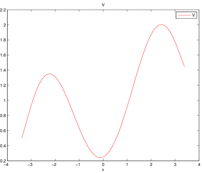
Figure 5.1: The three-well potential given by (5.80) on $D$.

For a temperature $\epsilon=0.5$, consider a diffusion $Y$ in such a potential starting at some $x_{0}\in D$. Let $\widetilde{{\tau}}$ be the hitting time of $Y$ of the boundary of $D$. Let $A=(-\infty,a_{1})$, $B=(a_{2},\infty)$, and let $\widetilde{{q}}_{1,a}=\widetilde{{q}}_{AB,a}$ and $\widetilde{{q}}_{2,a}=\widetilde{{q}}_{BA,a}$ (see Section 5.7), which for $a=0$ will be denoted simply as $\widetilde{{q}}_{1}$ and $\widetilde{{q}}_{2}$, and analogously in the Euler scheme case in which the tildes are omitted. Let us also consider $\widetilde{{\operatorname{mgf}}}$ and $\operatorname{mgf}$ for $p=\widetilde{{p}}:=0.1$. We computed approximations of such $\widetilde{{q}}_{i}(x)$ and $\widetilde{{\operatorname{mgf}}}(x)$ in the function of $x$ using finite difference discretizations of PDEs given by (5.66) and (5.67). The results are shown in figures 5.2a and 5.2b. In figures 5.3a and 5.3b we show approximations of the optimally tilted potentials (5.78) for the MGF and committors $\widetilde{{q}}_{i,a}$ for $a=0$ and $a=\widetilde{{a}}:=0.05$, $i=1,2$.

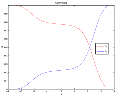
(a)

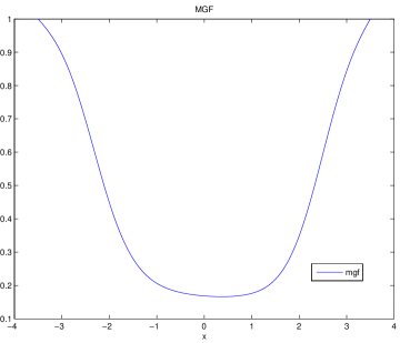
(b)

Figure 5.2: The committors and MGF as in the main text.

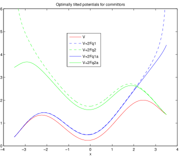
(a)

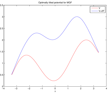
(b)

Figure 5.3: Optimally tilted potentials as in (5.78) for the MGF and committors. $Fqi$ and $Fqia$ are the functions $F$ as in Section 5.8 for the $i$th committor for $a=0$ and $a=\widetilde{{a}}$ respectively. The constant $C_{0}$ for the $i$th committor for $i\in\{1,2\}$ was chosen so that the tilted potential is equal to the original potential in point $a_{i}$ and for the MGF — so that these potentials are equal in both $a_{1}$ and $a_{2}$.

In our experiments we considered an Euler scheme $X$ with a time step $h=0.01$ corresponding to the above diffusion $Y$ starting at $x_{0}=0$. We focused on estimating $\operatorname{mgf}(x_{0})$ for $p=\widetilde{{p}}$, $q_{i}(x_{0})$ for $i=1,2$, and $p_{T}(x_{0})$ for $T=10$. For some $M\in\mathbb{N}_{2}$, $\widetilde{{a}}_{1}=-3.6$, $\widetilde{{a}}_{2}=3.6$, $\widetilde{{d}}=\frac{\widetilde{{a}}_{2}-\widetilde{{a}}_{1}}{M-1}$, and $p_{i}=\widetilde{{a}}_{1}+(i-1)\sigma$, $i\in\{1,\ldots,M\}$, consider Gaussian functions

$$\widetilde{{r}}_{i}(x)=\frac{1}{\sqrt{\epsilon}}\exp(-\frac{(x-p_{i})^{2}}{\widetilde{{d}}^{2}}),\quad i=1,\ldots,M.$$ (5.81)

In our experiments we used a linear parametrization of IS drifts as in Section 5.5. For each estimation problem we used as the IS basis functions the above Gaussian functions for $M=10$. For estimating $p_{T,a}(x_{0})$, considering a time-extended Euler scheme as in Remark 62 corresponding to the above $X$, we additionally performed experiments using $2M$ time-dependent IS basis functions

$$\widehat{{r}}_{i}(x,t)=\widetilde{{r}}_{i}(x),\ \widehat{{r}}_{M+i}(x,t)=t^{p}\widetilde{{r}}_{i}(x),\quad i=1,\ldots,M,$$ (5.82)

for different $p\in\mathbb{N}_{+}$, and for $M=5$ and $M=10$. See Section 7.1 and Chapter 10 for further details on our numerical experiments. Note that since the above $\widetilde{{r}}_{i}$ are continuous and $D$ is bounded, from remarks 64, 65, and Theorem 63, in which one can take $v=1$ and $\delta_{1}=\sqrt{2\epsilon}$, it follows that Condition 53 holds when estimating the MGF and committors as above. Using further the fact that $\mathbb{E}_{\widetilde{{\mathbb{U}}}}(\widetilde{{\tau}})<\infty$ (which follows e.g. from Lemma 7.4 in [31]), (5.72) holds. Furthermore, from Remark 66, we have (5.71) for the MGF and tanslated committors, and (5.75) for the exit probability.

Some properties of the minimized functions and their estimators

In this chapter we discuss various properties of the functions and their estimators from Chapter 4 for some parametrizations of IS from the previous chapter. These properties will be useful when proving the convergence and asymptotic properties of certain minimization methods of such estimators further on.

6.1 Cross-entropy and its estimators in the ECM setting

Let us consider the ECM setting as in Section 5.1. We have

$$\widehat{{\operatorname{ce}}}_{n}(b^{\prime},b)=\overline{(ZL^{\prime}(\Psi(b)-bX))}_{n}=\Psi(b)\overline{(ZL^{\prime})}_{n}-b^{T}\overline{(ZL^{\prime}X)}_{n}.$$ (6.1)

Let us assume Condition 36. Then,

$$\nabla_{b}\widehat{{\operatorname{ce}}}_{n}(b^{\prime},b)=\nabla\Psi(b)\overline{(ZL^{\prime})}_{n}-\overline{(ZL^{\prime}X)}_{n}$$ (6.2)

and

$$\nabla^{2}_{b}\widehat{{\operatorname{ce}}}_{n}(b^{\prime},b)=\nabla^{2}\Psi(b)\overline{(ZL^{\prime})}_{n}.$$ (6.3)

Let us further assume Condition 35, so that $\nabla^{2}\Psi$ is positive definite. Then, from (6.3), $b\to\widehat{{\operatorname{ce}}}_{n}(b^{\prime},b)(\omega)$ has a positive definite Hessian and thus it is strictly convex only for $\omega\in\Omega_{1}^{n}$ and $b^{\prime}\in A$ such that

$$\overline{(ZL^{\prime})}_{n}(\omega)>0.$$ (6.4)

Furthermore, $b^{*}_{n}\in A$ is the unique minimum point of $b\to\widehat{{\operatorname{ce}}}_{n}(b^{\prime},b)(\omega)$ only if (6.4) holds and

$$\nabla_{b}\widehat{{\operatorname{ce}}}_{n}(b^{\prime},b^{*}_{n})(\omega)=0$$ (6.5)

(where by $\nabla_{b}\widehat{{\operatorname{ce}}}_{n}(b^{\prime},b^{*}_{n})(\omega)$ we mean $\nabla_{b}(\widehat{{\operatorname{ce}}}_{n}(b^{\prime},b)(\omega))_{b=b^{*}_{n}}$). Assuming (6.4), from (6.2), (6.5) holds only if

$$\mu(b^{*}_{n})=\nabla\Psi(b^{*}_{n})=\frac{\overline{(ZL^{\prime}X)}_{n}}{\overline{(ZL^{\prime})}_{n}}(\omega),$$ (6.6)

or from Theorem 40 only if $\frac{\overline{(ZL^{\prime}X)}_{n}}{\overline{(ZL^{\prime})}_{n}}(\omega)\in\mu[A]$ and

$$b^{*}_{n}=\mu^{-1}\left(\frac{\overline{(ZL^{\prime}X)}_{n}}{\overline{(ZL^{\prime})}_{n}}(\omega)\right).$$ (6.7)

Let us assume that

$$\mathbb{E}_{\mathbb{Q}_{1}}(|ZX_{i}|)<\infty,\quad i=1,\ldots,l.$$ (6.8)

Due to $X$ having finite all mixed moments, from Hölder’s inequality, (6.8) holds e.g. when $\mathbb{E}_{\mathbb{Q}_{1}}(|Z|^{p})<\infty$ for some $p>1$. For the cross-entropy we then have

$$\operatorname{ce}(b)=\alpha\Psi(b)-b^{T}\mathbb{E}_{\mathbb{Q}_{1}}(ZX),\quad b\in A.$$ (6.9)

Thus, analogously as for the cross-entropy estimator above, $\operatorname{ce}$ has a positive definite Hessian everywhere only if $\alpha>0$, and $\operatorname{ce}$ has a unique minimum point only if $\alpha>0$ and

$$\frac{\mathbb{E}_{\mathbb{Q}_{1}}(ZX)}{\alpha}\in\mu[A],$$ (6.10)

in which case such a point is

$$b^{*}=\mu^{-1}\left(\frac{\mathbb{E}_{\mathbb{Q}_{1}}(ZX)}{\alpha}\right).$$ (6.11)

Remark 67.

Note that we can receive analogous conditions as above for the cross-entropy and its estimator to have negative definite Hessians or have unique maximum points by replacing $Z$ by $-Z$ (and thus also $\alpha$ by $-\alpha$) in the above conditions. The formulas for the maximum points remain the same as for the minimum points above. With some exceptions, in the further sections we shall focus on the minimization of cross-entropy and its estimators and will be interested in checking the conditions as in the main text above. However, we can analogously perform their maximization, or jointly optimization if we consider alternatives of the above conditions.

6.2 Some conditions in the LETS setting

Let $||\cdot||_{\infty}$ denote the supremum norm induced by the standard Euclidean norm $|\cdot|$. Consider the LETS setting as in Section 5.3.4. For each real matrix-valued process $Y=(Y_{k})_{k\in\mathbb{N}}$ on $\mathcal{{C}}$ and $B\in\mathcal{{E}}$, let us define

$$||Y||_{\tau,B,\infty}=\operatorname*{ess\,sup}_{\mathbb{U}}(\mathbb{1}_{B}\mathbb{1}(0<\tau<\infty)\max(||Y_{0}||_{\infty},\ldots,||Y_{\tau-1}||_{\infty})),$$ (6.12)

which for $B=\Omega_{1}$ is denoted simply as $||Y||_{\tau,\infty}$. Let $S$ be an $\overline{\mathbb{R}}$-valued random variable on $\mathcal{{S}}_{1}$. Further on in this work we will often assume the following conditions.

Condition 68.

It holds

$$R:=||\Lambda||_{\tau,S\neq 0,\infty}<\infty.$$ (6.13)

Condition 69.

A number $s\in\mathbb{N}_{+}$ is such that

$$\mathbb{1}(S\neq 0)\tau\leq s.$$ (6.14)

Note that conditions 68 or 69 hold for each possible random variable $S$ as above only if they hold for some $S$ such that $S(\omega)\neq 0$, $\omega\in\Omega_{1}$, that is only if

$$||\Lambda||_{\tau,\infty}<\infty$$ (6.15)

for Condition 68, or

$$\tau\leq s\in\mathbb{N}_{+}$$ (6.16)

for Condition 69.

Remark 70.

Note that Condition 69 implies Condition 52 for $Z=S$, while (6.16) implies Condition 53.

For each real matrix-valued function $f$ on $\mathbb{R}^{m}$ and $B\subset\mathbb{R}^{m}$, let us denote $||f||_{B,\infty}=\sup_{x\in B}||f||_{\infty}$. If $\tau$ is the exit time of an Euler scheme $X$ of a set $D$ such that $X_{0}\in D$, then for $\Lambda$ is as in (5.60) we have $||\Lambda||_{\tau,\infty}\leq||\Theta||_{D,\infty}$. In particular, if

$$||\Theta||_{D,\infty}<\infty,$$ (6.17)

then we have (6.15). Note that from (5.59), (6.17) is equivalent to $||\widetilde{{r}}_{i}||_{D,\infty}<\infty$, $i=1,\ldots,l$. In particular, (6.17) and thus also (6.15) hold in our numerical experiments as discussed in Section 5.9, both when using the time-independent and time-dependent IS basis functions, where in the time-dependent case by $\widetilde{{r}}_{i}$ we mean $\widehat{{r}}_{i}$ as in Section 5.9 and we consider $D$ equal to $\widehat{{D}}$ as in (5.74), $X$ equal to $X^{\prime}$ as in Remark 62, and $\tau$ equal to $\tau^{\prime}$ as in (5.73).

Let us discuss how one can enforce (6.16) if it is initially not fulfilled, as is the case for the translated committors and the MGF in our numerical experiments. Analogous reasonings as below can be applied also to more general stopped sequences or processes than in the LETS setting. For some $s\in\mathbb{N}_{+}$ and $z_{s}\in\mathbb{R}$, instead of $\tau$ and $Z$ we can consider their terminated versions $\tau_{s}=\tau\wedge s$ and $Z_{s}=\mathbb{1}(\tau\leq s)Z+z_{s}\mathbb{1}(\tau>s)$ and focus on computing $\alpha_{s}=\mathbb{E}_{\mathbb{U}}(Z_{s})=\mathbb{E}_{\mathbb{U}}(\mathbb{1}(\tau\leq s)Z)+z_{s}\mathbb{U}(\tau>s)$ rather than $\alpha=\mathbb{E}_{\mathbb{U}}(Z)$. If $\mathbb{U}(\tau=\infty)=0$, or $\mathbb{U}(Z\neq 0,\ \tau=\infty)=0$ and $\lim_{s\to\infty}z_{s}=0$, then $\mathbb{U}$ a.s. $Z_{s}\rightarrow Z$, so that assuming further that $\limsup_{s\to\infty}|z_{s}|<\infty$, from $|Z_{s}|\leq|Z|+|z_{s}|$ and Lebesgue’s dominated convergence theorem, $\lim_{s\rightarrow\infty}\alpha_{s}=\alpha$. Thus, in such a case, for a sufficiently large $s$ we will make arbitrarily small absolute error when approximating $\alpha$ by $\alpha_{s}$. Let us provide some upper bounds on this error. If $\operatorname*{ess\,sup}_{\mathbb{U}}(|Z-z_{s}|\mathbb{1}(\tau>s))\leq M_{s}\in[0,\infty)$, then

$$|\alpha-\alpha_{s}|=|\mathbb{E}_{\mathbb{U}}((Z-z_{s})\mathbb{1}(\tau>s))|\leq M_{s}\mathbb{U}(\tau>s).$$ (6.18)

For the MGF example from Section 5.7 we can take $z_{s}=M_{s}=\frac{1}{2}\exp(-ph(s+1))$, while for the translated committors we can choose $z_{s}=a+\frac{1}{2}$ and $M_{s}=\frac{1}{2}$. The quantity $\mathbb{U}(\tau>s)$ can be estimated using IS from the same simulations as used to estimate $\alpha_{s}$ or in a separate IS MC procedure. Alternatively, if we have $\tau\leq\widehat{{\tau}}$ for some random variable $\widehat{{\tau}}$ with a known distribution, we can use the inequality $\mathbb{U}(\tau>s)\leq\mathbb{U}(\widehat{{\tau}}>s)$ to bound the right side of (6.18) from above. For instance, if $\widehat{{\tau}}$ has a geometric distribution with a parameter $q$ (see Theorem 63 for a situation in which this may occur), then we have $\mathbb{U}(\widehat{{\tau}}>s)=(1-q)^{s}$ and thus $|\alpha-\alpha_{s}|\leq M_{s}(1-q)^{s}$.

6.3 Some conditions in the LETGS setting

Let us discuss some conditions and random conditions in the LETGS setting, which, as we shall discuss in the further sections, turn out to be necessary for the existence of the unique minimum points of cross-entropy, mean square, and their estimators in this setting. Let $Z$ be an $\mathbb{R}$-valued $\mathcal{{S}}_{1}$-measurable random variable (where $\mathcal{{S}}_{1}=(E,\mathcal{{F}}_{\tau})$).

Definition 71.

For $b\in A=\mathbb{R}^{l}$, we define a random condition $A_{b}$ on $\mathcal{{S}}_{1}$ as follows

$$A_{b}=(Z\neq 0,\ 0<\tau<\infty,\text{ and there exists }k\in\mathbb{N},\ k<\tau,\text{ such that }\lambda_{k}(b)\neq 0).$$ (6.19)

Lemma 72.

If $A_{b}$ does not hold and $Z\neq 0$, then for each $a\in\mathbb{R}^{l}$ and $t\in\mathbb{R}$

$$L(a+tb)=L(a).$$ (6.20)

Proof.

From (5.39), when $\tau=0$ then the both sides of (6.20) are equal to $1$ and when $\tau=\infty$ — to $\epsilon$. If $A_{b}$ does not hold, $Z\neq 0$, and $0<\tau<\infty$, then for each $0\leq k<\tau$ we have $\lambda_{k}(b)=0$, and thus for each $a\in\mathbb{R}^{l}$ and $t\in\mathbb{R}$, $\lambda_{k}(a+tb)=\lambda_{k}(a)+t\lambda_{k}(b)=\lambda_{k}(a)$, so that (6.20) also follows from (5.39). ∎

Lemma 73.

For $n\in\mathbb{N}_{+}$, the following random conditions on $\mathcal{{S}}_{1}^{n}$ are equivalent.

1. For each $b\in\mathbb{R}^{l},\ b\neq 0$, there exists $i\in\{1,\ldots,n\}$ such that $(A_{b})_{i}$ holds (where we use the notation as in (4.16)).

2. For some (equivalently, for each) random variable $K$ on $\Omega$ which is positive on $Z\neq 0$, $\overline{(\mathbb{1}(Z\neq 0)GK)}_{n}$ is positive definite.

3. It holds $N:=\sum_{i=1}^{n}\mathbb{1}(Z_{i}\neq 0,\ \tau_{i}<\infty)\tau_{i}>0$. Let a matrix $B\in\mathbb{R}^{(dN)\times l}$ be such that for each $i\in\{1,\ldots,n\}$ such that $0<\tau_{i}<\infty$ and $Z_{i}\neq 0$, for each $k\in\{0,\ldots,\tau_{i}-1\}$ and $j\in\{1,\ldots,d\}$ the $\sum_{v=1}^{i-1}\mathbb{1}(Z\neq 0,\ \tau_{v}<\infty)\tau_{v}+kd+j$th row of $B$ is equal to the $j$th row of $(\Lambda_{k})_{i}$. Then, the columns of $B$ are linearly independent.

Proof.

The fact that the second point above is a random condition follows from Sylvester’s criterion. The equivalence of the first two conditions follows from the fact that for each $b\in\mathbb{R}^{l}$

$$b^{T}\overline{(K\mathbb{1}(Z\neq 0)G)}_{n}b=\frac{1}{2n}\sum_{i=1}^{n}(\mathbb{1}(0<\tau<\infty,\ Z\neq 0)K\sum_{k=0}^{\tau-1}|\lambda_{k}(b)|^{2})_{i}$$ (6.21)

and the equivalence of the first and last condition is obvious. ∎

Definition 74.

We define $r_{n}$ to be one of the equivalent random conditions in Lemma 73.

Lemma 75.

The below three conditions are equivalent.

1. For each $b\in\mathbb{R}^{l}$, $b\neq 0$, we have $\mathbb{Q}_{1}(A_{b})>0$.

2. For each $b\in\mathbb{R}^{l}$, from $\mathbb{Q}_{1}(A_{b})=0$ it follows that $b=0$.

3. Let $\widetilde{{\Lambda}}_{j}=((\Lambda_{k,i,j})_{i=1}^{d})_{k\in\mathbb{N}}\in\mathcal{{J}}$, $j=1,\ldots,l$ (see Definition 42). Let $\sim$ be a relation of equivalence on $\mathcal{{J}}$ such that for $\psi_{1},\psi_{2}\in\mathcal{{J}}$, $\psi_{1}\sim\psi_{2}$, only if $\mathbb{Q}_{1}$ a.s. if $0<\tau<\infty$ and $Z\neq 0$ then $\psi_{1,i}=\psi_{2,i}$, $i=0,\ldots,\tau-1$. Then, the equivalence classes $[\widetilde{{\Lambda}}_{1}]_{\sim},\ldots,[\widetilde{{\Lambda}}_{l}]_{\sim}$ are linearly independent in the linear space $\mathcal{{J}}/\mathord{\sim}$ of equivalence classes of $\sim$, defined in a standard way (i.e. the operations in such a linear space are defined by using in them in the place of the equivalence classes their arbitrary members and then taking the equivalence class of the result).

Proof.

The equivalence of the first two conditions is obvious. The equivalence of the last two conditions follows from the fact that, using notations as in the third condition, for $b\in\mathbb{R}^{l}$, $\sum_{i=1}^{l}b_{i}\widetilde{{\Lambda}}_{i}$ is equal to the zero in $\mathcal{{J}}/\mathord{\sim}$ only if $\mathbb{Q}_{1}(A_{b})=0$. ∎

Condition 76.

We define the condition under consideration to be one of the conditions from Lemma 75.

Remark 77.

Note that for a probability $\mathbb{S}\sim_{\tau<\infty}\mathbb{Q}_{1}$ we have $\mathbb{S}(A_{b})>0$ only if $\mathbb{Q}_{1}(A_{b})>0$, so that Condition 76 holds only if it holds for such a $\mathbb{S}$ in the place of $\mathbb{Q}_{1}$.

Remark 78.

Note that $\mathbb{Q}_{1}(A_{b})>0$ only if for some $l\in\mathbb{N}_{+}$ and $k\in\mathbb{N}$, $k<l$, we have $\mathbb{Q}_{1}(Z\neq 0,\ \tau=l,\ \lambda_{k}(b)\neq 0)>0$.

Lemma 79.

Let for some probability $\mathbb{S}\sim_{\tau<\infty}\mathbb{Q}_{1}$, a random variable $K$ on $\mathcal{{S}}_{1}$ be $\mathbb{S}$ a.s. positive on $Z\neq 0$, and let $\mathbb{1}(Z\neq 0)KG$ have $\mathbb{S}$-integrable entries. Then, $\mathbb{E}_{\mathbb{S}}(\mathbb{1}(Z\neq 0)KG)$ is positive definite only if Condition 76 holds.

Proof.

For each $b\in\mathbb{R}^{l}$, $b\neq 0$,

$$b^{T}\mathbb{E}_{\mathbb{S}}(\mathbb{1}(Z\neq 0)KG)b=\frac{1}{2}\mathbb{E}_{\mathbb{S}}(\mathbb{1}(Z\neq 0,\ 0<\tau<\infty)K\sum_{k=0}^{\tau-1}|\lambda_{k}(b)|^{2})$$ (6.22)

is greater than zero only if $\mathbb{S}(A_{b})>0$, so that from Remark 77 we receive the thesis. ∎

Let $\operatorname{Sym}_{n}(\mathbb{R})$ denote the subset of $\mathbb{R}^{n\times n}$ consisting of symmetric matrices, and let $m_{n}:\operatorname{Sym}_{n}(\mathbb{R})\to\mathbb{R}$ be such that for $A\in\operatorname{Sym}_{n}(\mathbb{R})$, $m_{n}(A)$ is equal to the lowest eigenvalue of $A$, or equivalently

$$m_{n}(A)=\inf_{x\in\mathbb{R}^{n},\ |x|=1}x^{T}Ax.$$ (6.23)

Lemma 80.

$m_{n}$ is Lipschitz from $(\operatorname{Sym}_{n}(\mathbb{R}),||\cdot||_{\infty})$ to $(\mathbb{R},|\cdot|)$ with a Lipschitz constant $1$.

Proof.

For $A,B\in\operatorname{Sym}_{n}(\mathbb{R})$ and $x\in\mathbb{R}^{n}$, $|x|=1$, we have $x^{T}Ax=x^{T}Bx+x^{T}(A-B)x$, so that

$$x^{T}Bx-||A-B||_{\infty}\leq x^{T}Ax\leq x^{T}Bx+||A-B||_{\infty}$$ (6.24)

and thus

$$m_{n}(B)-||A-B||_{\infty}\leq m_{n}(A)\leq m_{n}(B)+||A-B||_{\infty}$$ (6.25)

and

$$|m_{n}(B)-m_{n}(A)|\leq||A-B||_{\infty}.$$ (6.26)

∎

Lemma 81.

If the entries of some matrices $M_{n}\in\operatorname{Sym}_{l}(\mathbb{R})$, $n\in\mathbb{N}_{+}$, converge to the respective entries of a positive definite symmetric matrix $M\in\mathbb{R}^{l\times l}$, then for a sufficiently large $n$, $M_{n}$ is positive definite.

Proof.

This follows from the fact that $A\in\operatorname{Sym}_{l}(\mathbb{R})$ is positive definite only if $m_{l}(A)>0$, and from Lemma 80, $\lim_{n\to\infty}m_{l}(M_{n})=m_{l}(M)$. ∎

Theorem 82.

If Condition 76 holds, then under Condition 32, a.s. for a sufficiently large $n$, $r_{n}(\widetilde{{\kappa}}_{n})$ holds for $r_{n}$ as in Definition 74. In particular, a.s. $\lim_{n\rightarrow\infty}\mathbb{P}(r_{n}(\widetilde{{\kappa}}_{n}))=1$.

Proof.

Let $K=\exp(-\max_{i,j=1,\ldots,d}|G_{i,j}|)$. Then, $K>0$ and the entries of the matrix $\mathbb{1}(Z\neq 0)GK$ are bounded and thus $\mathbb{Q}^{\prime}$-integrable. Thus, from Lemma 79 for $\mathbb{S}=\mathbb{Q}^{\prime}$, $\mathbb{E}_{\mathbb{Q}^{\prime}}(\mathbb{1}(Z\neq 0)KG)$ is positive definite. Let $A_{n}=\overline{(\mathbb{1}(Z\neq 0)KG)}_{n}(\widetilde{{\kappa}}_{n})$. From the SLLN, a.s.

$$\lim_{n\rightarrow\infty}A_{n}=\mathbb{E}_{\mathbb{Q}^{\prime}}(\mathbb{1}(Z\neq 0)KG).$$ (6.27)

Thus, from Lemma 81, a.s. $A_{n}$ is positive definite for a sufficiently large $n$ and the thesis follows from the second point of Lemma 73. ∎

6.4 Discussion of Condition 76 in the Euler scheme case

Let us consider IS for an Euler scheme with a linear parametrization of IS drifts, discussed in Section 5.5 below formula (5.57). In this section we shall reformulate Condition 76 and provide some sufficient assumptions for it to hold in such a case.

Let us define a measure $\nu$ on $\mathcal{{S}}(\mathbb{R}^{m})$ to be such that for each $B\in\mathcal{{B}}(\mathbb{R}^{m})$

$$\begin{split}\nu(B)&=\mathbb{E}_{\mathbb{U}}(\mathbb{1}(Z\neq 0,\ 0<\tau<\infty)\sum_{k=0}^{\tau-1}\mathbb{1}(X_{k}\in B))\\ &=\sum_{l\in\mathbb{N}_{+}}\sum_{k=0}^{l-1}\mathbb{U}(Z\neq 0,\ \tau=l,\ X_{k}\in B)\\ &=\sum_{k=0}^{\infty}\mathbb{U}(Z\neq 0,\ k<\tau<\infty,\ X_{k}\in B).\\ \end{split}$$ (6.28)

Remark 83.

From the second line of (6.28), Remark 78, and (5.60), $\mathbb{Q}_{1}(A_{b})=\mathbb{U}(A_{b})=0$ is equivalent to

$$\nu(\{\Theta b\neq 0\})=0$$ (6.29)

(where $\{\Theta b\neq 0\}=\{x\in\mathbb{R}^{m}:\Theta(x)b\neq 0\}$).

Remark 84.

Let for each $i\in\{1,\ldots,l\}$, $\widetilde{{\Theta}}_{i}:\mathbb{R}^{m}\rightarrow\mathbb{R}^{d}$ be the $i$th column of $\Theta$ and $[\widetilde{{\Theta}}_{i}]_{\approx}$ be the class of equivalence of $\widetilde{{\Theta}}_{i}$ with respect to the relation $\approx$ of equality $\nu$ a.e. on the set $\mathcal{{K}}$ of measurable functions from $\mathcal{{S}}(\mathbb{R}^{m})$ to $\mathcal{{S}}(\mathbb{R}^{d})$. Then, from Remark 83, Condition 76 is equivalent to $[\widetilde{{\Theta}}_{i}]_{\approx}$, $i=1,\ldots,l$, being linearly independent in the linear space $\mathcal{{K}}/\mathord{\approx}$ defined in a standard way.

Let us assume that $m=n+1$ for some $n\in\mathbb{N}_{+}$. Consider the following condition concerning the IS basis functions $\widetilde{{r}}_{i}:\mathbb{R}^{m}\to\mathbb{R}^{d}$, $i=1,\ldots,l$, as in Section 5.5.

Condition 85.

For some $m_{1},m_{2}\in\mathbb{N}_{+}$, functions $g_{1,i}:\mathbb{R}\to\mathbb{R}$, $i=1,\ldots,m_{1}$, and $g_{2,i}:\mathbb{R}^{n}\to\mathbb{R}^{d}$, $i=1,\ldots,m_{2}$, are such that for $K_{1}=\{kh:k\in\{1,\ldots,m_{1}\}\}$, $g_{1,i|K_{1}}$, $i=1,\ldots,m_{1}$, are linearly independent and for each $i\in\{1,\ldots,m_{1}\}$, for some open set $K_{2,i}\subset\mathbb{R}^{n}$, $g_{2,j|K_{2,i}}$, $j=1,\ldots,m_{2}$, are continuous and linearly independent. Furthermore, we have $l=m_{1}m_{2}$, and denoting $\pi(i,j)=m_{2}(i-1)+j$, for each $x\in\mathbb{R}^{n}$ and $t\in\mathbb{R}$ we have $\widetilde{{r}}_{\pi(i,j)}(x,t)=g_{1,i}(t)g_{2,j}(x)$, $i=1,\ldots,m_{1}$, $j=1,\ldots,m_{2}$.

Remark 86.

As the functions $g_{1,i}$ as in the above condition one can take for example polynomials $g_{1,i}(t)=t^{i-1}$, $i=1,\ldots,m_{1}$. For $m_{1}=2$ one can also use $g_{1,1}(t)=1$ and $g_{1,2}(t)=t^{p}$ for some $p\in\mathbb{N}_{+}$. For $n=1$ and arbitrary nonempty open sets $K_{2,i}\subset\mathbb{R}$, $i=1,\ldots,m_{2}$, as the functions $g_{2,i}$ in the above condition one can take e.g. polynomials analogously as above or Gaussian functions $g_{2,i}(x)=a_{i}\exp(\frac{(x-p_{i})^{2}}{s})$ for some $a_{i}\in\mathbb{R}\setminus\{0\}$, $s\in\mathbb{R}_{+}$, and $p_{i}\in R$ different for different $i$ (the linear independence of such Gaussian functions on each open interval can be proved by an analogous reasoning as in [1]). In particular, for such $K_{2,i}$, Condition 85 holds for the functions $\widetilde{{r}}_{i}$ equal to $\widehat{{r}}_{i}$ as in (5.82) or equal to $\widehat{{r}}_{i}$ such that $\widehat{{r}}_{i}(x,t)=\widetilde{{r}}_{i}(x)$, $x\in\mathbb{R}^{n}$, $t\in\mathbb{R}$, for $\widetilde{{r}}_{i}$ as in (5.81), where in the first case $m_{1}=2$, in the second $m_{1}=1$, and in both cases $n=1$ and $m_{2}$ is equal to $M$ as in Section 5.9.

Let $\lambda$ denote the Lebesgue measure on $\mathbb{R}^{n}$ and $\delta_{x}$ — the Dirac measure centred on $x$.

Theorem 87.

If Condition 85 holds and

$$\lambda\otimes\delta_{ih}\ll_{K_{2,i}\times\{ih\}}\nu,\quad i=1,\ldots,m_{1},$$ (6.30)

then Condition 76 holds.

Proof.

Let $b\in\mathbb{R}^{l}$ be such that $\mathbb{U}(A_{b})=0$. Then, from Remark 83, $\nu(\{\Theta b\neq 0\})=0$ and thus for $i=1,\ldots,m_{1}$, $\nu(\{(x,ih):x\in K_{2,i},\ \Theta(x,ih)b\neq 0\})=0$ and from (6.30)

$$\lambda(\{x\in K_{2,i}:\Theta(x,ih)b\neq 0\})=0.$$ (6.31)

From (5.59) and Condition 85 we have for $x\in\mathbb{R}^{n}$ and $t\in\mathbb{R}$

$$\Theta(x,t)b=\sqrt{h}\sum_{j=1}^{m_{1}}\sum_{k=1}^{m_{2}}b_{\pi(j,k)}g_{1,j}(t)g_{2,k}(x).$$ (6.32)

Denoting for $i=1,\ldots,m_{1}$ and $k=1,\ldots,m_{2}$

$$a_{i,k}=\sum_{j=1}^{m_{1}}b_{\pi(j,k)}g_{1,j}(ih),$$ (6.33)

we thus have $\Theta(x,ih)b=\sqrt{h}\sum_{k=1}^{m_{2}}a_{i,k}g_{2,k}(x)$, $x\in\mathbb{R}^{n}$, and from (6.31),

$$\lambda(\{x\in K_{2,i}:\sum_{k=1}^{m_{2}}a_{i,k}g_{2,k}(x)\neq 0\})=0.$$ (6.34)

Thus, for $i=1,\ldots,m_{1}$, from the continuity and linear independence of $g_{2,k|K_{2,i}}$ , $k=1,\ldots,m_{2}$, we have $a_{i,k}=0$, $k=1,\ldots,m_{2}$. Therefore, from (6.33), for $k=1,\ldots,m_{2}$, $\sum_{j=1}^{m_{1}}b_{\pi(j,k)}g_{1,j|K_{1}}=0$, so that from the linear independence of $g_{1,j|K_{1}}$, $j=1,\ldots,m_{1}$, we have $b=0$. ∎

Let us assume the following condition.

Condition 88.

We have $\sigma_{m,i}=0$, $i=1,\ldots,d$, $\mu_{m}=1$, $(x_{0})_{m}=0$, and $\widetilde{{\sigma}}:\mathbb{R}^{m}\to\mathbb{R}^{n\times d}$ is such that $\widetilde{{\sigma}}_{i,j}=\sigma_{i,j}$, $i=1,\ldots,n$, $j=1,\ldots,d$.

Note that it now holds for $\widetilde{{X}}_{k}=(X_{k,i})_{i=0}^{n}$, $k\in\mathbb{N}$, that

$$X_{k}=(\widetilde{{X}}_{k},kh),\quad k\in\mathbb{N}.$$ (6.35)

For $x\in\mathbb{R}^{n}$ and $k\in\mathbb{N}$ for which $\widetilde{{\sigma}}(x,kh)$ has linearly independent rows, let $Q_{k}(x)=(h\widetilde{{\sigma}}(x,kh)\widetilde{{\sigma}}(x,kh)^{T})^{-1}$, and for $y\in\mathbb{R}^{n}$, let

$$\rho_{k}(x,y)=\frac{\sqrt{\det(Q_{k}(x))}}{(2\pi)^{\frac{m}{2}}}\exp((y-x-h\mu(x))^{T}Q_{k}(y-x-h\mu(x))).$$ (6.36)

Theorem 89.

Let $k\in\mathbb{N}_{+}$ and sets $B_{1},B_{2},\ldots,B_{k},C\in\mathcal{{B}}(\mathbb{R}^{n})$ have positive Lebesgue measure. Let $\mathbb{U}$ a.s. the fact that $\widetilde{{X}}_{i}\in B_{i},\ i=1,\ldots,k$ and $\widetilde{{X}}_{k+1}\in C$ imply that $Z\neq 0$ and $k<\tau<\infty$. Let further $\widetilde{{\sigma}}(x,t)$ have independent rows for each $(x,t)\in\{x_{0}\}\cup\bigcup_{i=1}^{k}B_{i}\times\{ih\}$. Then,

$$\lambda\otimes\delta_{ih}\ll_{B_{i}\times\{ih\}}\nu,\quad i=1,\ldots,k.$$ (6.37)

Proof.

It follows from the fact that for each $j\in\{1,\ldots,k\}$, for each $D\subset\mathcal{{B}}(B_{j})$ such that $\lambda(D)>0$, for $\widetilde{{D}}=\prod_{i=1}^{j-1}B_{i}\times D\times\prod_{i=j+1}^{k}B_{i}\times C$ we have

$$\begin{split}0&<\int_{\widetilde{{D}}}\prod_{i=0}^{k}\rho_{i}(x_{i},x_{i+1})\,\mathrm{d}x_{1}\,\mathrm{d}x_{2}\ldots\,\mathrm{d}x_{k+1}\\ &=\mathbb{U}((\widetilde{{X}}_{i})_{i=1}^{k+1}\in\widetilde{{D}})\\ &=\mathbb{U}(Z\neq 0,\ k<\tau<\infty,\ (\widetilde{{X}}_{i})_{i=1}^{k+1}\in\widetilde{{D}})\\ &\leq\mathbb{U}(Z\neq 0,\ j<\tau<\infty,\ \widetilde{{X}}_{j}\in D)\\ &\leq\nu(D\times\{jh\}),\\ \end{split}$$ (6.38)

where in the last line we used (6.35) and the last line of (6.28). ∎

Remark 90.

Let us consider the problems of estimating an MGF $\operatorname{mgf}(x_{0})$, a translated committor $q_{AB,a}(x_{0})$, and a translated exit probability by a given time $p_{T,a}(x_{0})$ as in Section 5.7 for $a\neq-1$. As $x_{0}$, $\mu$, and $\sigma$ fulfilling the above Condition 88 let us consider $x_{0}^{\prime}$, $\mu^{\prime}$, and $\sigma^{\prime}$ as in Remark 62, and as an Euler scheme $X$ in the LETGS setting as above let us consider the time-extended process $X^{\prime}$ as in that remark. Note that the process $X$ as in Section 5.7 is now equal to the above $\widetilde{{X}}$. Let $k\in\mathbb{N}_{+}$. Then for $D$ and $Z$ corresponding to the above expectations as in Section 5.7, assuming that $C\in\mathcal{{B}}(B)$ in the case of estimation of the translated committor, or $C\in\mathcal{{B}}(D^{\prime})$ for the MGF or the exit probability, and additionally $T\geq h(k+1)$ in the case of the exit probability, for each $B\in\mathcal{{B}}(D)$ we have that $\widetilde{{X}}_{i}\in B,\ i=1,\ldots,k$ and $\widetilde{{X}}_{k+1}\in C$ implies that $Z\neq 0$ and $\tau=k+1$ (where for the exit probability rather than $\tau$ we mean $\tau^{\prime}$ as in (5.73)). This holds also for $Z$ and $\tau$ replaced by their terminated versions $Z_{s}$ and $\tau_{s}$ for $s\in\mathbb{N}_{+}$, $s>k$, as in Section 6.2.

From remarks 86 and 90 and theorems 87 and 89 it follows that Condition 76 holds in all the cases considered in our numerical experiments as in Section 5.9 if for the case of the exit probability before a given time we assume that $T\geq h(m_{1}+1)$ for $m_{1}$ depending on the basis functions used as in Remark 86. Furthermore, this condition also holds in such terminated cases as in Section 6.2 for each $s\in\mathbb{N}_{+}$, $s>m_{1}$.

6.5 Cross-entropy and its estimators in the LETGS setting

Consider the LETGS setting. From (5.43),

$$\begin{split}\widehat{{\operatorname{ce}}}_{n}(b^{\prime},b)&=\overline{ZL^{\prime}(b^{T}Gb+Hb+\mathbb{1}(\tau=\infty)\ln(\epsilon))}_{n}\\ &=b^{T}\overline{(ZL^{\prime}G)}_{n}b+\overline{(ZL^{\prime}H)}_{n}b+\ln(\epsilon)\overline{(ZL^{\prime}\mathbb{1}(\tau=\infty))}_{n},\\ \end{split}$$ (6.39)

so that

$$\nabla_{b}\widehat{{\operatorname{ce}}}_{n}(b^{\prime},b)=2\overline{(ZL^{\prime}G)}_{n}b+\overline{(ZL^{\prime}H)}_{n}.$$ (6.40)

Thus, $b\rightarrow\widehat{{\operatorname{ce}}}_{n}(b^{\prime},b)(\omega)$ has a unique minimum point $b^{*}_{n}\in A$ only for $\omega\in\Omega_{1}^{n}$ for which $\overline{(ZL^{\prime}G)}_{n}(\omega)$ is positive definite, in which case for $A_{n}(b^{\prime}):=2\overline{(ZL^{\prime}G)}_{n}$ and $B_{n}(b^{\prime}):=-\overline{(ZL^{\prime}H)}_{n}$ we have

$$b^{*}_{n}=(A_{n}(b^{\prime}))^{-1}(\omega)B_{n}(b^{\prime})(\omega).$$ (6.41)

Note that if $Z\geq 0$ then from the second point of Lemma 73 for $K=ZL^{\prime}$, for each $\omega\in\Omega_{1}^{n}$, $\overline{(ZL^{\prime}G)}_{n}(\omega)$ is positive definite only if $r_{n}(\omega)$ holds (see Definition 74).

Condition 91.

$ZG$ and $ZH$ have $\mathbb{Q}_{1}$-integrable (equivalently, $\mathbb{U}$-integrable) entries.

Lemma 92.

Let Condition 68 hold for $S=Z$, let for some $p>1$, $\mathbb{E}_{\mathbb{U}}(|Z|^{p})<\infty$, and let for some $s\in\mathbb{N}_{+}$ and a random variable $\widehat{{\tau}}$ with a geometric distribution under $\mathbb{U}$ with a parameter $q\in(0,1]$ it hold

$$\mathbb{1}(Z\neq 0)\tau\leq\widetilde{{\tau}}:=s+\widehat{{\tau}}.$$ (6.42)

Then, for each $1\leq u<p$, we have $\mathbb{E}_{\mathbb{U}}(|ZH_{i}|^{u})<\infty$ and $\mathbb{E}_{\mathbb{U}}(|ZG_{i,j}|^{u})<\infty$, $i,j\in\{1,\ldots,l\}$. In particular, Condition 91 holds.

Proof.

Let $1\leq u<p$. For $r\in(u,\infty)$ such that $\frac{u}{r}+\frac{u}{p}=1$, using Hölder’s inequality and (6.42) we have

$$\mathbb{E}_{\mathbb{U}}(|Z||G||_{\infty}|^{u})\leq\mathbb{E}_{\mathbb{U}}((|Z|\tau\frac{1}{2}R^{2})^{u})\leq(\frac{1}{2}R^{2})^{u}(\mathbb{E}_{\mathbb{U}}(|Z|^{p}))^{\frac{u}{p}}(\mathbb{E}_{\mathbb{U}}(\widetilde{{\tau}}^{r}))^{\frac{u}{r}}<\infty$$ (6.43)

and

$$\mathbb{E}_{\mathbb{U}}((|Z||H||_{\infty}|)^{u})\leq\mathbb{E}_{\mathbb{U}}((|Z|R\sum_{k=1}^{\tau}|\eta_{k}|)^{u})\leq R^{u}(\mathbb{E}_{\mathbb{U}}(Z^{p}))^{\frac{u}{p}}(\mathbb{E}_{\mathbb{U}}((\sum_{k=1}^{\widetilde{{\tau}}}|\eta_{k}|)^{r}))^{\frac{u}{r}}.\\$$ (6.44)

Furthermore,

$$\mathbb{E}_{\mathbb{U}}((\sum_{k=1}^{\widetilde{{\tau}}}|\eta_{k}|)^{r})=\sum_{l=1}^{\infty}\mathbb{E}_{\mathbb{U}}(\mathbb{1}(\widetilde{{\tau}}=l)(\sum_{k=1}^{l}|\eta_{k}|)^{r})\leq\sum_{l=1}^{\infty}l^{r-1}\mathbb{E}_{\mathbb{U}}(\mathbb{1}(\widetilde{{\tau}}=l)\sum_{k=1}^{l}|\eta_{k}|^{r})\\$$ (6.45)

and from Schwarz’s inequality,

$$\mathbb{E}_{\mathbb{U}}(\mathbb{1}(\widetilde{{\tau}}=l)\sum_{k=1}^{l}|\eta_{k}|^{r})\leq\mathbb{U}(\widetilde{{\tau}}=l)^{\frac{1}{2}}(\mathbb{E}_{\mathbb{U}}((\sum_{k=1}^{l}|\eta_{k}|^{r})^{2}))^{\frac{1}{2}}.$$ (6.46)

It holds $\mathbb{U}(\widetilde{{\tau}}=s+k)=q(1-q)^{k-1}$, $k\in\mathbb{N}_{+}$, and $\mathbb{E}_{\mathbb{U}}((\sum_{k=1}^{l}|\eta_{k}|^{r})^{2})=l\mathbb{E}_{\mathbb{U}}(|\eta_{1}|^{2r}+l(l-1)(\mathbb{E}_{\mathbb{U}}(|\eta_{1}|^{r}))^{2}$. The thesis easily follows from the above formulas. ∎

Note that (6.42) in the above lemma holds e.g. for $s=0$ and $\widehat{{\tau}}$ as in Theorem 63 if the assumptions of this theorem hold for $B=\{0\}$, or for $\widehat{{\tau}}=0$ for $\tau$ being an arbitrary stopping time terminated at $s$ as in Section 6.2.

Let us assume conditions 52 and 91. Then, from (5.43) we receive the following formula for the cross-entropy

$$\operatorname{ce}(b)=\mathbb{E}_{\mathbb{Q}_{1}}(Z\ln(L(b)))=b^{T}\mathbb{E}_{\mathbb{Q}_{1}}(ZG)b+\mathbb{E}_{\mathbb{Q}_{1}}(ZH)b.$$ (6.47)

Let $\widetilde{{A}}=2\mathbb{E}_{\mathbb{Q}_{1}}(ZG)=\nabla^{2}\operatorname{ce}(b)$, $b\in\mathbb{R}^{l}$, and $\widetilde{{B}}=-\mathbb{E}_{\mathbb{Q}_{1}}(ZH)$. Then, we have $\nabla\operatorname{ce}(b)=\widetilde{{A}}b-\widetilde{{B}}$. Thus, if $\mathbb{E}_{\mathbb{Q}_{1}}(ZG)$ is positive definite, then $\operatorname{ce}$ has a unique point $b^{*}\in A$, satisfying

$$b^{*}=\widetilde{{A}}^{-1}\widetilde{{B}}.$$ (6.48)

If $Z\geq 0$, then from Lemma 79 for $K=Z$, $\mathbb{E}_{\mathbb{Q}_{1}}(ZG)$ is positive definite only if Condition 76 holds. Remark 67 applies also to the above discussion in the LETGS setting.

6.6 Some properties of expectations of random functions

Some of the below theorems are modifications or slight extensions of well-known results; see the appendix of Chapter 1 in [53].

Let $l\in\mathbb{N}_{+}$ and $A\in\mathcal{{B}}(\mathbb{R}^{l})$ be nonempty. A function $f:A\to\overline{\mathbb{R}}$ is said to be lower semicontinuous in a point $b\in A$ if $\liminf_{x\to b}f(x)\geq f(b)$, and it is said to be lower semicontinuous if it is lower semicontinuous in each $b\in A$.

Lemma 93.

A lower semicontinuous function $f:A\to\overline{\mathbb{R}}$ such that $f>-\infty$ (i.e. $f(b)>-\infty$, $b\in A$) attains a minimum on each nonempty compact set $K\subset A$ (where such a minimum may be equal to infinity).

Proof.

Let $m=\inf_{b\in K}f(b)$ and let $a_{n}\in K$, $n\in\mathbb{N}_{+}$, be such that $\lim_{n\rightarrow\infty}f(a_{n})=m$. Consider a subsequence $(a_{n_{k}})_{k\in\mathbb{N}_{+}}$ of $(a_{n})_{n\in\mathbb{N}_{+}}$, converging to some $b^{*}\in K$. Then, from the lower semicontinuity of $f$, $m=\liminf_{k\rightarrow\infty}f(a_{n_{k}})\geq f(b^{*})$, so that $f(b^{*})=m$. ∎

Condition 94.

A (random) function $h:\mathcal{{S}}(A)\otimes(\Omega,\mathcal{{F}})\to\mathcal{{S}}(\overline{\mathbb{R}})$ is such that a.s. $b\ inA\to h(b):=h(b,\cdot)$ is lower semicontinuous and

$$\mathbb{E}(\sup_{b\in A}(h(b)_{-}))<\infty.$$ (6.49)

For such a $h$ we denote $b\in A\to f(b):=\mathbb{E}(h(b))$.

Lemma 95.

Assuming Condition 94, we have $f>-\infty$ and $f$ is lower semicontinuous on $A$.

Proof.

From (6.49), $f>-\infty$. For each $b\in A$ and $a_{n}\in A$, $n\in\mathbb{N}$, such that $\lim_{n\to\infty}a_{n}=b$, from Fatou’s lemma (which can be used thanks to (6.49)) and the a.s. lower semicontinuity of $b\rightarrow h(b)$,

$$\liminf_{n\to\infty}f(a_{n})\geq\mathbb{E}(\liminf_{n\rightarrow\infty}h(a_{n}))\geq f(b).$$ (6.50)

∎

Let further in this section $A\subset\mathbb{R}^{l}$ be open. For $x\in A$, let $d_{x}=\inf_{y\in A^{\prime}}|y-x|$. For a sequence $x_{n}\in A$, $n\in\mathbb{N}_{+}$, let us write $x_{n}\uparrow A$ if $\max(\frac{1}{d_{x_{n}}},\ |x_{n}|)\to\infty$ as $n\to\infty$, i.e. $x_{n}$ in a sense tries to leave $A$. For $a\in\overline{\mathbb{R}}$ and $f:A\to\overline{\mathbb{R}}$, let us denote by $\lim_{x\uparrow A}f(x)=a$ the fact that $\lim_{n\to\infty}f(x_{n})=a$ whenever $x_{n}\uparrow A$.

Condition 96.

A lower semicontinuous function $f:A\to\overline{\mathbb{R}}$ fulfills $f>-\infty$ and $\lim_{x\uparrow A}f(x)=\infty$.

Condition 97.

Condition 96 holds, the set $B$ on which $f$ is finite is nonempty and convex, and $f$ is strictly convex on $B$.

Lemma 98.

Under Condition 96, $f$ attains a minimum on $A$ and if Condition 97 holds, then the corresponding minimum point $b^{*}$ is unique and $f(b^{*})<\infty$.

Proof.

Under Condition 96, for a sufficiently large $M>0$, for a compact set

$$K=\{b\in A:|b|\leq M,\ d_{b}\geq\frac{1}{M}\},$$ (6.51)

we have $\inf_{b\in A}f(b)=\inf_{b\in K}f(b)$. From Lemma 93 there exists a minimum point $b^{*}\in K$ of $f$ on $K$ and thus also on $A$. Under Condition 97 we have $f(b^{*})<\infty$ and the uniqueness of $b^{*}$ follows from the strict convexity of $f$. ∎

Lemma 99.

Assuming Condition 94, if with positive probability $\lim_{b\uparrow A}h(b)=\infty$, then $\lim_{b\uparrow A}f(b)=\infty$.

Proof.

For $a_{k}\uparrow A$, from Fatou’s lemma

$$\liminf_{k\rightarrow\infty}f(a_{k})\geq\mathbb{E}(\liminf_{k\rightarrow\infty}h(a_{k}))=\infty.$$ (6.52)

∎

Lemma 100.

Under Condition 94, let us assume that $A$ is convex, for some $b_{0}\in A$, $f(b_{0})<\infty$, and a.s. $b\rightarrow h(b)$ is convex. Then, $f$ is convex on the convex nonempty set $B\subset A$ on which it is finite. If further with positive probability $b\rightarrow h(b)\in\mathbb{R}$ is strictly convex and $\lim_{b\uparrow A}h(b)=\infty$, then $f$ satisfies Condition 97.

Proof.

The (strict) convexity of $f$ and the convexity of $B$ easily follow from $f(b)=\mathbb{E}(h(b))$. The remaining points of Condition 97 follow from lemmas 95 and 99. ∎

6.7 Some properties of mean square and its estimators

Let us consider the mean square function and its estimators as in sections 4.1 and 4.2 (under appropriate assumptions as in these sections).

Condition 101.

$A$ is convex and $b\in A\to L(b)(\omega)\in\mathbb{R}$ is convex and continuous, $\omega\in\Omega_{1}$.

From (4.21), if Conditon 101 holds, then $b\to\widehat{{\operatorname{msq}}}_{n}(b^{\prime},b)$ is convex and continuous (for each $b^{\prime}\in A$ and when evaluated on each $\omega\in\Omega_{1}^{n}$).

Definition 102.

For $A$ open and convex, let the random condition $p_{\operatorname{msq}}$ on $\mathcal{{S}}_{1}$ hold only if $Z\neq 0$, $b\to L(b)\in\mathbb{R}_{+}$ is strictly convex, and $\lim_{b\uparrow A}L(b)=\infty$.

Remark 103.

If Condition 101 holds and for some $n\in\mathbb{N}_{+}$, $\omega=(\omega_{i})_{i=1}^{n}\in\Omega_{1}^{n}$, and $i\in\{1,\ldots,n\}$, $p_{\operatorname{msq}}(\omega_{i})$ holds, then for each $b^{\prime}\in A$, $b\to\widehat{{\operatorname{msq}}}_{n}(b^{\prime},b)(\omega)\in\mathbb{R}$ is strictly convex, continuous, and $\lim_{b\uparrow A}\widehat{{\operatorname{msq}}}_{n}(b^{\prime},b)(\omega)=\infty$.

It holds

$$\widehat{{\operatorname{msq}2}}_{n}(b^{\prime},b)=\frac{1}{n^{2}}\sum_{i=1}^{n}\left(Z_{i}^{2}L_{i}^{\prime}L_{i}(b)\sum_{j\in\{1,\ldots,n\},j\neq i}\frac{L_{j}^{\prime}}{L_{j}(b)}\right)+\frac{1}{n}\overline{((ZL^{\prime})^{2})}_{n}.$$ (6.53)

Thus, $b\to\widehat{{\operatorname{var}}}_{n}(b^{\prime},b)$ and $b\to\widehat{{\operatorname{msq}2}}_{n}(b^{\prime},b)$ are positively linearly equivalent to $b\to f_{\operatorname{var},n}(b^{\prime},b)$ for

$$f_{\operatorname{var},n}(b^{\prime},b)=\sum_{i=1}^{n}\left(Z_{i}^{2}L_{i}^{\prime}\sum_{j\in\{1,\ldots,n\},j\neq i}\frac{L_{j}^{\prime}L_{i}(b)}{L_{j}(b)}\right),\quad b^{\prime},b\in A.$$ (6.54)

Condition 104.

For each $\omega_{1},\omega_{2}\in\Omega_{1}$, $b\to\frac{L(b)(\omega_{1})}{L(b)(\omega_{2})}$ is convex.

Note that if Condition 104 holds, then $b\to f_{\operatorname{var},n}(b^{\prime},b)$ is convex and thus so are $b\to\widehat{{\operatorname{var}}}_{n}(b^{\prime},b)$ and $b\to\widehat{{\operatorname{msq}2}}_{n}(b^{\prime},b)$.

Remark 105.

Let us assume Condition 32 and that $b\in A\to L(b)(\omega)\in\mathbb{R}$ is continuous, $\omega\in\Omega_{1}$. Then, for each $n\in\mathbb{N}_{+}$, from $\widehat{{\operatorname{msq}}}_{n}$ being nonnegative, Condition 94 holds for $h(b,\cdot)=\widehat{{\operatorname{msq}}}_{n}(b^{\prime},b)(\widetilde{{\kappa}}_{n})$, for which $f=\operatorname{msq}$ in that condition.

Lemma 106.

Under Condition 101, if $\mathbb{Q}_{1}(p_{\operatorname{msq}})>0$ and for some $b\in A$, $\operatorname{msq}(b)<\infty$, then $f=\operatorname{msq}$ satisfies Condition 97.

Proof.

It follows from Remark 103, Remark 105 for $n=1$, and Lemma 100. ∎

6.8 Mean square and its estimators in the ECM setting

Let us consider the ECM setting as in Section 5.1 for $A$ open. As discussed there, for each $\omega\in\Omega_{1}$, $b\to L(b)(\omega)$ is convex, and under Condition 35, $b\to L(b)(\omega)$ is strictly convex. Thus, under Condition 35, for each $\omega\in\Omega_{1}$, $p_{\operatorname{msq}}(\omega)$ holds (see Definition (102)) only if $Z(\omega)\neq 0$ and $\lim_{b\uparrow A}L(b)(\omega)=\infty$. Note that for $X$ having a non-degenerate normal distribution under $\mathbb{Q}_{1}$, for each $\omega\in\Omega_{1}$, $\lim_{|b|\to\infty}L(b)(\omega)=\infty$, so that $p_{\operatorname{msq}}$ holds only if $Z\neq 0$. For $X$ having the distribution of a product of $n$ exponentially tilted distributions from the gamma family under $\mathbb{Q}_{1}$, we have $\mathbb{Q}_{1}(X\in\mathbb{R}_{+}^{n})=1$, and for $\omega\in\Omega_{1}$ such that $X(\omega)\in\mathbb{R}_{+}^{n}$, we have $L(b)(\omega)\to\infty$ as $b\uparrow A$. Thus, for such an $\omega$, $p_{\operatorname{msq}}(\omega)$ holds only if $Z(\omega)\neq 0$, and the condition $\mathbb{Q}_{1}(p_{\operatorname{msq}})>0$, appearing in Lemma 106, reduces to $\mathbb{Q}_{1}(Z\neq 0)>0$. For $X$ having a Poisson distribution under $\mathbb{Q}_{1}$, we have $\lim_{|b|\to\infty}L(b)(\omega)=\infty$ when $X(\omega)\in\mathbb{N}_{+}$, but not when $X(\omega)=0$. Thus, in such a case $p_{\operatorname{msq}}$ holds when $Z\neq 0$ and $X\in\mathbb{N}_{+}$, but not when $X=0$, and we have $\mathbb{Q}_{1}(p_{\operatorname{msq}})>0$ only if $\mathbb{Q}_{1}(X\in\mathbb{N}_{+},\ Z\neq 0)>0$.

Remark 107.

Let us assume Condition 36. Then, for each $n\in\mathbb{N}_{+}$ and $b^{\prime}\in A$,

$$\nabla_{b}\widehat{{\operatorname{msq}}}_{n}(b^{\prime},b)=\overline{(Z^{2}L^{\prime}(\mu(b)-X)L(b))}_{n}$$ (6.55)

and

$$\nabla^{2}_{b}\widehat{{\operatorname{msq}}}_{n}(b^{\prime},b)=\overline{(Z^{2}L^{\prime}(\Sigma(b)+(\mu(b)-X)(\mu(b)-X)^{T})L(b))}_{n}.$$ (6.56)

Let us further in this remark assume Condition 35, so that $\Sigma(b)$ is positive definite. Then, for $\omega\in\Omega_{1}^{n}$ such that $Z(\omega_{i})\neq 0$ for some $i\in\{1,\ldots,n\}$, $\nabla^{2}_{b}\widehat{{\operatorname{msq}}}_{n}(b^{\prime},b)(\omega)$ is positive definite for each $b^{\prime},b\in A$. Indeed, in such a case for each $v\in\mathbb{R}^{l}\setminus\{0\}$ we have

$$\begin{split}v^{T}\nabla^{2}_{b}\widehat{{\operatorname{msq}}}_{n}(b^{\prime},b)v&=v^{T}\Sigma(b)v\overline{(Z^{2}L^{\prime}L(b))}_{n}+\overline{(Z^{2}L^{\prime}L(b)((\mu(b)-X)^{T}v)^{2})}_{n}\\ &\geq v^{T}\Sigma(b)v\overline{(Z^{2}L^{\prime}L(b))}_{n}>0.\\ \end{split}$$ (6.57)

Note that Condition 104 holds for ECM since for each $\omega_{1},\omega_{2}\in\Omega_{1}$ and $b\in A$ we have

$$\frac{L(b)(\omega_{1})}{L(b)(\omega_{2})}=\exp(b^{T}(X(\omega_{2})-X(\omega_{1}))).$$ (6.58)

In particular, as discussed in the previous section, the estimators of variance and the new estimators of mean square are convex. For each $n\in\mathbb{N}_{+}$, $\omega\in\Omega_{1}^{n}$, and $i,j\in\{1,\ldots,n\}$, let us denote

$$v_{j,i}(\omega)=X(\omega_{j})-X(\omega_{i}).$$ (6.59)

For each $n\in\mathbb{N}_{2}$, let a function $g_{\operatorname{var},n}:A\times\mathbb{R}^{l}\times\Omega_{1}^{n}\to\mathbb{R}$ be such that for each $b^{\prime}\in A$, $b\in\mathbb{R}^{l}$, and $\omega\in\Omega_{1}^{n}$

$$g_{\operatorname{var},n}(b^{\prime},b)(\omega)=\sum_{i=1}^{n}\left((Z^{2}L^{\prime})(\omega_{i})\sum_{j\in\{1,\ldots,n\},j\neq i}L^{\prime}(\omega_{j})\exp(b^{T}v_{j,i}(\omega))\right).$$ (6.60)

Note that for each $b^{\prime}$ and $\omega$ as above, $b\in\mathbb{R}^{l}\to g_{\operatorname{var},n}(b^{\prime},b)(\omega)$ is convex and

$$g_{\operatorname{var},n}(b^{\prime},b)(\omega)=f_{\operatorname{var},n}(b^{\prime},b)(\omega),\quad b\in A.$$ (6.61)

For $A=\mathbb{R}^{l}$, we have $g_{\operatorname{var},n}=f_{\operatorname{var},n}$, but in some cases, like for the gamma family of distributions as in Section 5.1, we have $A\neq\mathbb{R}^{l}$ and $f_{\operatorname{var},n}$ is only a restriction of $g_{\operatorname{var},n}$. For each $b^{\prime}$, $b$, and $\omega$ as above, it holds

$$\nabla_{b}g_{\operatorname{var},n}(b^{\prime},b)(\omega)=\sum_{i=1}^{n}\left((Z^{2}L^{\prime})(\omega_{i})\sum_{j\in\{1,\ldots,n\},j\neq i}L^{\prime}(\omega_{j})v_{j,i}(\omega)\exp(b^{T}v_{j,i}(\omega))\right)$$ (6.62)

and

$$\nabla^{2}_{b}g_{\operatorname{var},n}(b^{\prime},b)(\omega)=\sum_{i=1}^{n}\left((Z^{2}L^{\prime})(\omega_{i})\sum_{j\in\{1,\ldots,n\},j\neq i}L^{\prime}(\omega_{j})v_{j,i}(\omega)v_{j,i}(\omega)^{T}\exp(b^{T}v_{j,i}(\omega))\right).$$ (6.63)

Let $n\in\mathbb{N}_{2}$ and $\omega\in\Omega_{1}^{n}$. Let $D(\omega)\in\mathbb{R}^{l\times n^{2}}$ be a matrix whose $(i-1)n+j$th column, $i,j\in\{1,\ldots,n\}$, is equal to $\mathbb{1}(Z\neq 0)(\omega_{i})v_{j,i}(\omega)$.

Lemma 108.

If $D(\omega)$ has linearly independent rows, then for each $b\in\mathbb{R}^{l}$ and $b^{\prime}\in A$, $\nabla^{2}_{b}g_{\operatorname{var},n}(b^{\prime},b)(\omega)$ is positive definite.

Proof.

If $D(\omega)$ has linearly independent rows, then for each $t\in\mathbb{R}^{l}$, $t\neq 0$, there exist $i,j\in\{1,\ldots,n\}$, $i\neq j$, such that $t^{T}\mathbb{1}(Z\neq 0)(\omega_{i})v_{j,i}(\omega)\neq 0$, so that from (6.63),

$$t^{T}\nabla^{2}_{b}g_{\operatorname{var},n}(b^{\prime},b)(\omega)t\geq(Z^{2}L^{\prime})(\omega_{i})L^{\prime}(\omega_{j})(t^{T}v_{j,i}(\omega))^{2}\exp(b^{T}v_{j,i}(\omega))>0.$$ (6.64)

∎

Let for each $k\in\{1,\ldots,n\}$ a matrix $\widetilde{{D}}(k,\omega)\in\mathbb{R}^{l\times(n-1)}$ have the consecutive columns equal to $v_{k,j}(\omega)$ for $j=1,2,\ldots,k-1,k+1,k+2,\ldots,n$.

Lemma 109.

$D(\omega)$ has linearly independent rows only if for some $i\in\{1,\ldots,n\}$, $Z(\omega_{i})\neq 0$, and for some (equivalently, for each) $k\in\{1,\ldots,n\}$, $\widetilde{{D}}(k,\omega)$ has linearly independent rows.

Proof.

If $Z(\omega_{i})=0$, $i=1,\ldots,n$, then $D(\omega)$ has zero rows, so that they are linearly dependent. The dimensions of the linear spans of the columns and vectors of a matrix are the same, so that the matrices $D(\omega)$ and $\widetilde{{D}}(k,\omega)$, $k\in\{1,\ldots,n\}$, have linearly independent rows only if the dimension of the linear span of their columns is equal to $l$. Thus, the thesis follows from the easy to check fact that the linear span $V$ of the columns of $\widetilde{{D}}(k,\omega)$ for different $k\in\{1,\ldots,n\}$ is the same and if $Z(\omega_{i})\neq 0$ for some $i\in\{1,\ldots,n\}$, then the linear span of the columns of $D(\omega)$ is equal to $V$. ∎

For a vector $v\in\mathbb{R}^{m}$, by $v\leq 0$ we mean that its coordinates are nonpositive.

Theorem 110.

If the system of linear inequalities

$$D^{T}(\omega)b\leq 0,\quad b\in\mathbb{R}^{l},$$ (6.65)

has only the zero solution, then for each $b^{\prime}\in A$, $g_{\operatorname{var},n}(b^{\prime},b)(\omega)\to\infty$ as $|b|\to\infty$ and $\nabla^{2}_{b}g_{\operatorname{var},n}(b^{\prime},b)(\omega)$ is positive definite, $b\in\mathbb{R}^{l}$. If $b$ is a solution of (6.65), then for each $b^{\prime}\in A$, $a\in\mathbb{R}^{l}$, and $t\in[0,\infty)$, we have

$$g_{\operatorname{var},n}(b^{\prime},a+tb)(\omega)\leq g_{\operatorname{var},n}(b^{\prime},a)(\omega).$$ (6.66)

Proof.

For $b\in\mathbb{R}^{l}$ for which (6.65) holds, for $i\in\{1,\ldots,n\}$ such that $Z(\omega_{i})\neq 0$, for $j\in\{1,\ldots,n\}$, $i\neq j$, we have $b^{T}v_{j,i}(\omega)\leq 0$, so that (6.66) follows from (6.60). Let further (6.65) have only the zero solution. Then, $D(\omega)$ has linearly independent rows, and thus the positive definiteness of $\nabla^{2}_{b}g_{\operatorname{var},n}(b^{\prime},b)(\omega)$ follows from Lemma 108. Consider a function $b\in\mathbb{R}^{l}\to f(b):=\max\{b^{T}v_{j,i}(\omega):Z(\omega_{i})\neq 0,\ i,j\in\{1,\ldots,n\},\ i\neq j\}$. Then, for each $b\in\mathbb{R}^{l}$, $b\neq 0$, it holds $f(b)>0$. Thus, from the continuity of $f$ we have $0<\delta:=\min\{f(b):|b|=1\}$ and for $0<a:=\min\{(Z^{2}L^{\prime})(\omega_{i})L^{\prime}(\omega_{j}):Z(\omega_{i})\neq 0,\ i,j\in\{1,\ldots,n\},\ i\neq j\}$, from (6.60)

$$g_{\operatorname{var},n}(b^{\prime},b)(\omega)\geq a\exp(\delta|b|)\to\infty$$ (6.67)

as $|b|\to\infty$. ∎

There exist numerical methods for finding the set of solutions of (6.65) and in particular for checking if it has only the zero solution; see [33].

Theorem 111.

Let us assume that

$$Z(\omega_{i})\neq 0,\quad i=1\ldots,n.$$ (6.68)

Then, (6.65) has only the zero solution only if $D(\omega)$ has linearly independent rows, which from Lemma 109 holds only if for some (equivalently, for each) $k\in\{1,\ldots,n\}$, $\widetilde{{D}}(k,\omega)$ has linearly independent rows.

Proof.

Assuming (6.68), for $b\in\mathbb{R}^{l}$, $D^{T}(\omega)b\leq 0$ holds only if

$$v_{i,j}(\omega)^{T}b\leq 0,\quad i,j\in\{1,\ldots,n\}.$$ (6.69)

Since $v_{i,j}(\omega)=-v_{j,i}(\omega)$, this holds only if $v_{i,j}(\omega)^{T}b=0$, $i,j\in\{1,\ldots,n\}$, i.e. only if $D^{T}(\omega)b=0$. ∎

6.9 Strongly convex functions and $\epsilon$-minimizers

For some nonempty $A\subset\mathbb{R}^{l}$, consider a function $f:A\to\overline{\mathbb{R}}$. For some $\epsilon\geq 0$, we say that $x^{*}\in A$ is an $\epsilon$-minimizer of $f$, if

$$f(x^{*})\leq\inf_{x\in A}f(x)+\epsilon.$$ (6.70)

Consider a convex set $S\subset A$, such that $A$ is a neighbourhood of $S$ (i.e. $S$ is contained in some open set $D\subset A$). Then, $f$ is said to be strongly convex on $S$ (where we do not mention $S$ if it is equal to $A$) with a (strong convexity) constant $m>0$, if $f$ is twice differentiable on $S$ and for each $b\in\mathbb{R}^{l}$ and $x\in S$

$$b^{T}\nabla^{2}f(x)b\geq m|b|^{2}.$$ (6.71)

Let us discuss some properties of strongly convex functions $f$ on $S$ as above (see Section 9.1.2. in [9] for more details). It is well known that $f$ as above is strictly convex on $S$, and from Taylor’s theorem it easily follows that for $x,y\in S$

$$f(y)\geq f(x)+(\nabla f(x))^{T}(y-x)+\frac{m}{2}|y-x|^{2}.$$ (6.72)

In particular, $f(y)\to\infty$ as $|y|\to\infty$, $y\in S$. Furthermore, if $\nabla f(x)=0$, then

$$f(y)\geq f(x)+\frac{m}{2}|y-x|^{2}.$$ (6.73)

Thus, $x$ is a unique minimum point of $f_{|S}$ only if $\nabla f(x)=0$. The right-hand side of (6.72) in the function of $y\in\mathbb{R}^{l}$ is minimized by $\widetilde{{y}}=x-\frac{1}{m}\nabla f(x)$, and thus we have

$$f(y)\geq f(x)+(\nabla f(x))^{T}(\widetilde{{y}}-x)+\frac{m}{2}|\widetilde{{y}}-x|^{2}=f(x)-\frac{1}{2m}|\nabla f(x)|^{2}.$$ (6.74)

Let $f$ have a unique minimum point $b^{*}\in S$. Then, from (6.74) for $y=b^{*}$, for $x\in S$ we have

$$f(x)\leq f(b^{*})+\frac{1}{2m}|\nabla f(x)|^{2}.$$ (6.75)

In particular, each $x\in S$ is a $\frac{1}{2m}|\nabla f(x)|^{2}$-minimizer of $f$.

6.10 Mean square and its well-known estimators in the LETGS setting

Let us in this section consider the LETGS setting.

Theorem 112.

Let $b^{\prime},b\in\mathbb{R}^{l}$, $n\in\mathbb{N}_{+}$, and $\omega\in\Omega_{1}^{n}$. Then, $b\in\mathbb{R}^{l}\to f(b):=\widehat{{\operatorname{msq}}}_{n}(b^{\prime},b)(\omega)$ is convex and if $r_{n}(\omega)$ holds (see Definition 74), then $f$ is strongly convex. If $r_{n}(\omega)$ does not hold, then there exists $b\in\mathbb{R}^{l}\setminus\{0\}$ such that

$$f(a+tb)=f(a),\quad a\in\mathbb{R}^{l},\ t\in\mathbb{R}.$$ (6.76)

Proof.

It holds

$$\nabla^{2}f(b)=\overline{(Z^{2}L^{\prime}(2G+(2Gb+H)(2Gb+H)^{T})L(b))}_{n}(\omega),$$ (6.77)

which is positive semidefinite, so that $f$ is convex. If $r_{n}(\omega)$ does not hold, then from the first point of Lemma 73 there exists $b\in\mathbb{R}^{l}$ such that for each $i\in 1,\ldots,n,$, $A_{b}(\omega_{i})$ does not hold, so that from Lemma 72 and (4.21) we receive (6.76). Let us assume that $r_{n}(\omega)$ holds. Then, from the second point of Lemma 73 for $K=Z^{2}L^{\prime}$, the matrix $M:=\overline{(Z^{2}L^{\prime}G)}_{n}(\omega)$ is positive definite. Let $m_{1}>0$ be such that $b^{T}Mb\geq m_{1}|b|^{2}$, $b\in\mathbb{R}^{l}$. For each $i\in\{1,\ldots,n\}$ such that $\tau(\omega_{i})<\infty$, from Remark 59 we have

$$m_{2,i}:=\inf_{b\in\mathbb{R}^{l}}L(b)(\omega_{i})=\exp(\inf_{b\in\mathbb{R}^{l}}\ln(L(b)(\omega_{i})))\in\mathbb{R}_{+}.$$ (6.78)

Let $m_{2}=\min\{m_{2,i}:i\in\{1,\ldots,n\},\ \tau(\omega_{i})<\infty\}$. Then, $m_{2}\in\mathbb{R}_{+}$ and for each $a,b\in\mathbb{R}^{l}$ we have

$$a^{T}\nabla^{2}f(b)a\geq 2a^{T}\overline{(Z^{2}L^{\prime}GL(b))}_{n}(\omega)a\geq 2m_{2}a^{T}\overline{(Z^{2}L^{\prime}G)}_{n}(\omega)a\geq 2m_{1}m_{2}|a|^{2}.$$ (6.79)

∎

Theorem 113.

If conditions 32 and 76 hold, then a.s. for a sufficiently large $n$, $b\rightarrow\widehat{{\operatorname{msq}}}_{n}(b^{\prime},b)(\widetilde{{\kappa}}_{n})$ is strongly convex. In particular, the probability of this event converges to one as $n\to\infty$.

Proof.

It follows directly from theorems 82 and 112. ∎

Theorem 114.

Let Condition 52 hold. If $\operatorname{msq}(b_{0})<\infty$ for some $b_{0}\in\mathbb{R}^{l}$, then $\operatorname{msq}$ is convex on the convex nonempty set $B$ on which it is finite and if further Condition 76 holds, then $f=\operatorname{msq}$ satisfies Condition 97 (in particular, from Lemma 98, it has a unique minimum point). If Condition 76 does not hold, then there exists $b\in\mathbb{R}^{l}$, $b\neq 0$, such that

$$\operatorname{msq}(a+tb)=\operatorname{msq}(a),\quad a\in\mathbb{R}^{l},\ t\in\mathbb{R}.$$ (6.80)

Proof.

The first part of the thesis follows from theorems 112 and 113, the properties of strongly convex functions discussed in Section 6.9, Remark 105, and, under Condition 32, from Lemma 100 for $h(b,\cdot)=\widehat{{\operatorname{msq}}}_{n}(b^{\prime},b)(\widetilde{{\kappa}}_{n})$ for a sufficiently large $n$. If Condition 76 does not hold, then there exists $b\in\mathbb{R}^{l}$, $b\neq 0$, such that $\mathbb{Q}_{1}(A_{b})=0$, for which (6.80) follows from Lemma 72 and formula (4.9). ∎

6.11 Smoothness of functions in the LETS setting

In this section we provide some sufficient conditions for the smoothness and for certain properties of the derivatives of functions defined in Section 4.1. Unless stated otherwise, we consider the LETS setting, which contains the LETGS setting as a special case (see Section 5.3.4). From Remark 61, the ECM setting for $A=\mathbb{R}^{l}$ can be identified with the LETS setting for $\tau=1$ and $\Lambda_{0}=I_{l}$, so that it is easy to modify the below theory to deal also with such an ECM setting.

Condition 115.

A measurable function $S:\mathcal{{S}}_{1}\to\mathcal{{S}}(\overline{\mathbb{R}})$ is such that conditions 68 and 69 hold and for each $\theta\in(\mathbb{R}^{d})^{s}$

$$\mathbb{E}_{\mathbb{U}}(|S|\exp(\sum_{i=1}^{s}\theta_{i}^{T}\widetilde{{X}}(\eta_{i})))<\infty.$$ (6.81)

Note that Condition 115 implies that $S$ is $\mathbb{U}$-integrable.

Remark 116.

In the special case which can be identified with the ECM setting for $A=\mathbb{R}^{l}$ as discussed above, Condition 68 holds for $R=1$ and Condition 69 holds for $s=1$. Thus, for some $S:\mathcal{{S}}_{1}\to\mathcal{{S}}(\overline{\mathbb{R}})$, a counterpart of Condition 115 in the ECM setting for $A=\mathbb{R}^{l}$ reduces to demanding that

$$\mathbb{E}_{\mathbb{U}}(|S|\exp(\theta^{T}X))<\infty,\quad\theta\in\mathbb{R}^{l}.$$ (6.82)

Remark 117.

Since for each $s\in\mathbb{N}_{+}$ and $\theta\in(\mathbb{R}^{d})^{s}$, $\mathbb{E}_{\mathbb{U}}(\exp(\sum_{i=1}^{s}\theta_{i}^{T}\widetilde{{X}}(\eta_{i})))=\exp(\sum_{i=1}^{s}\widetilde{{\Psi}}(\theta_{i}))<\infty$, from Hölder’s inequality, (6.81) holds if we have $\mathbb{E}_{\mathbb{U}}(|S|^{q})<\infty$ for some $q\in(1,\infty)$.

Condition 118.

We have $t,s\in\mathbb{N}_{+}$ and $f:(\mathcal{{S}}(\mathbb{R}^{l}))^{t}\otimes\mathcal{{C}}\to\mathcal{{S}}(\mathbb{R})$ is such that for each $M\in\mathbb{R}_{+}$, for some $N\in\mathbb{N}_{+}$, $\phi\in((\mathbb{R}^{d})^{s})^{N}$, and $u\in\mathbb{R}_{+}^{N}$, we have $\mathbb{U}$ a.s.

$$\sup_{b\in(\mathbb{R}^{l})^{t}:|b_{i}|\leq M,\ i=1,\ldots,t}|f(b)|\leq\sum_{i=1}^{N}u_{i}\exp(\sum_{j=1}^{s}\phi_{i,j}^{T}\widetilde{{X}}(\eta_{j}))$$ (6.83)

(where $f(b)=f(b,\cdot)$).

Remark 119.

Let Condition 118 hold and $S$ satisfy Condition 115 (for the same $s$). Let $M\in\mathbb{R}_{+}$ and consider the corresponding $N$, $\phi$, and $u$ as in Condition 118. Then, for each $\theta\in(\mathbb{R}^{d})^{s}$

$$\mathbb{E}_{\mathbb{U}}(\sup_{b\in(\mathbb{R}^{l})^{t}:|b_{i}|\leq M,\ i=1,\ldots,t}|Sf(b)\exp(\sum_{j=1}^{s}\theta_{j}^{T}\widetilde{{X}}(\eta_{j}))|)\leq\sum_{i=1}^{N}u_{i}\mathbb{E}_{\mathbb{U}}(S\exp(\sum_{j=1}^{s}(\phi_{i,j}+\theta_{j})^{T}\widetilde{{X}}(\eta_{j})))<\infty.$$ (6.84)

In particular, $\mathbb{E}_{\mathbb{U}}(\sup_{b\in(\mathbb{R}^{l})^{t}:|b_{i}|\leq M,\ i=1,\ldots,t}|Sf(b)|)<\infty$. Furthermore, from the above $M\in\mathbb{R}_{+}$ being arbitrary, for each $b\in(\mathbb{R}^{l})^{t}$, $Sf(b)$ satisfies Condition 115.

In this work we assume that $x^{0}=1,\ x\in\mathbb{R}$.

Theorem 120.

Let conditions 68 and 69 hold, let $t\in\mathbb{N}_{+}$, $r\in\mathbb{R}^{t}$, $w\in\mathbb{N}^{t\times l}$, $u\in\mathbb{N}^{t\times s\times d}$, $z\in\mathbb{N}^{t\times s\times d\times l}$, $y\in\mathbb{N}_{+}^{t\times s}$, $v\in\prod_{m=1}^{t}\prod_{i=1}^{s}(\mathbb{N}^{l})^{y_{m,i}}$, and $q\in\prod_{m=1}^{t}\prod_{i=1}^{s}\mathbb{N}^{y_{m,i}}$. Let for each $b\in(\mathbb{R}^{l})^{t}$

$$\begin{split}f(b)&=\mathbb{1}(S\neq 0)|\prod_{m=1}^{t}(L(b_{m})^{r_{m}}\prod_{i=1}^{l}b_{m,i}^{w_{m,i}}\prod_{i=1}^{\tau\wedge s}(\prod_{j=1}^{d}(\widetilde{{X}}_{j}(\eta_{i})^{u_{m,i,j}}\\ &\cdot\prod_{k=1}^{l}(\Lambda_{i-1})_{j,k}^{z_{m,i,j,k}})\prod_{j=1}^{y_{m,i}}(\partial_{v_{m,i,j}}\widetilde{{\Psi}}(\lambda_{i-1}(b_{m})))^{q_{m,i,j}}))|.\end{split}$$ (6.85)

Then, Condition 118 holds for such an $f$ (for the same $t$ and $s$ as above).

Proof.

Let $M\in[0,\infty)$ and $g(x)=e^{x}+e^{-x}$. For $p\in\mathbb{R}$ and $b\in\mathbb{R}^{l}$, $|b|\leq M$, from (5.42) we have $\mathbb{U}$ a.s.

$$\mathbb{1}(S\neq 0)L^{p}(b)\leq K(p):=\exp(|p|s\widetilde{{F}}(RM))\prod_{i=1}^{s}\prod_{j=1}^{d}g(pRM\widetilde{{X}}_{j}(\eta_{i})).$$ (6.86)

Let for $x\in[0,\infty)$ and $a\in\mathbb{N}^{l}$

$$U_{a}(x)=1+\sup_{b\in\mathbb{R}^{l},\ |b|\leq x}|\partial_{a}\widetilde{{\Psi}}(b)|,$$ (6.87)

which is finite thanks to Remark 37. Then, for each $b\in(\mathbb{R}^{l})^{t}$, $|b_{i}|\leq M$, $i=1,\ldots,m$, we have $\mathbb{U}$ a.s.

$$\begin{split}|f(b)|&\leq\mathbb{1}(S\neq 0)\prod_{m=1}^{t}(K(r_{m})M^{\sum_{i=1}^{l}w_{m,i}}\prod_{i=1}^{s}(\prod_{j=1}^{d}(g(\widetilde{{X}}_{j}(\eta_{i}))^{u_{m,i,j}}(1+R)^{\sum_{k=1}^{l}z_{m,i,j,k}})\\ &\cdot\prod_{j=1}^{y_{m,i}}U_{v_{m,i,j}}(RM)^{q_{m,i,j}})).\end{split}$$ (6.88)

The right-hand side of (6.88) can be rewritten to have the form as the right-hand side of (6.83). ∎

Theorem 121.

If conditions 68 and 69 hold, then for each $t\in\mathbb{N}_{+}$, $p_{1},p_{2}\in\mathbb{R}^{t}$ such that $p_{2,i}\geq 1$, $i=1,\ldots,t$, $M\in\mathbb{R}_{+}$, $v\in(\mathbb{N}^{l})^{t}$, and for $h_{p_{1},p_{2}}(b,\omega):=(\mathbb{1}(S\neq 0)\prod_{i=1}^{t}|\partial_{v_{i}}(L^{p_{1,i}}(b_{i}))|^{p_{2,i}})(\omega)$, $b\in(\mathbb{R}^{l})^{t}$, $\omega\in E$, Condition 118 holds for $f=h_{p_{1},p_{2}}$.

Proof.

Since for $p_{3}\in(\mathbb{N}_{+})^{t}$ such that $p_{3,i}\geq p_{2,i}$, $i=1,\ldots,t$, we have

$$|h_{p_{1},p_{2}}(b)|\leq\mathbb{1}(S\neq 0)\prod_{i=1}^{t}(1+|\partial_{v_{i}}(L^{p_{1,i}}(b_{i}))|)^{p_{3,i}},$$ (6.89)

it is sufficient to prove the above theorem for $p_{2}\in\mathbb{N}_{+}^{t}$. In such a case $h_{p_{1},p_{2}}(b)$ is a linear combination of a finite number of variables as in (6.85). Thus, the thesis follows from Theorem 120. ∎

Theorem 122.

If Condition 115 holds, then for each $p\in\mathbb{R}$, for $g(b)=SL^{p}(b)$, $b\in\mathbb{R}^{l}\to f(b)=\mathbb{E}_{\mathbb{U}}(g(b))\in\mathbb{R}$ is smooth and we have $\partial_{v}f(b)=\mathbb{E}_{\mathbb{U}}(\partial_{v}g(b))$, $v\in\mathbb{N}^{l}$, $b\in\mathbb{R}^{l}$.

Proof.

It follows from Theorem 121 for $p_{1}=p$ and $p_{2}=1$ and from Remark 119 by induction over $\sum_{i=1}^{l}v_{i}$ using mean value and Lebesgue’s dominated convergence theorems. ∎

Theorem 123.

If Condition 115 holds

1. for $S=1$, then $1=\mathbb{E}_{\mathbb{U}}(L^{-1}(b))$ and for each $v\in\mathbb{N}^{l}$, $v\neq 0$, $\mathbb{E}_{\mathbb{U}}(\partial_{v}(L^{-1}(b)))=0$, $b\in\mathbb{R}^{l}$,

2. for $S=Z^{2}$, then $\operatorname{msq}$ is smooth and $\partial_{v}\operatorname{msq}(b)=\mathbb{E}_{\mathbb{U}}(Z^{2}\partial_{v}L(b))$, $b\in\mathbb{R}^{l}$, $v\in\mathbb{N}^{l}$,

3. for $S=C$, then $b\to c(b)$ is smooth and $\partial_{v}c(b)=\mathbb{E}_{\mathbb{U}}(C\partial_{v}(L^{-1}(b)))=\mathbb{E}_{\mathbb{U}}(\mathbb{1}(C\neq\infty)C\partial_{v}(L^{-1}(b)))$, $b\in\mathbb{R}^{l}$, $v\in\mathbb{N}^{l}$,

4. for $S$ equal to $Z^{2}$ and $C$, then $\operatorname{ic}$ is smooth.

Proof.

The first three points follow from Theorem 122 and from the fact that due to remarks 70 and 54, we have $1=\mathbb{E}_{\mathbb{U}}(L(b)^{-1})$, $\operatorname{msq}(b)=\mathbb{E}_{\mathbb{U}}(Z^{2}L(b))$, and $c(b)=\mathbb{E}_{\mathbb{U}}(CL^{-1}(b))$ respectively, $b\in\mathbb{R}^{l}$, and in the third point additionally (4.27). The last point is a consequence of points two and three. ∎

Theorem 124.

In the ECM setting for $A=\mathbb{R}^{l}$, let us assume that $\mathbb{Q}_{1}(Z\neq 0)>0$, conditions 35 and 36 hold, and we have (6.82) for $S=Z^{2}$. Then, $\nabla^{2}\operatorname{msq}(b)$ exists and is positive definite, $b\in\mathbb{R}^{l}$.

Proof.

From a counterpart of Theorem 120 and Remark 119 for ECM, $W=Z^{2}L(b)(\mu(b)-X)(\mu(b)-X)^{T}$ has integrable entries. Thus, from the second point of a counterpart of Theorem 123 for ECM

$$\begin{split}\nabla^{2}\operatorname{msq}(b)&=\mathbb{E}_{\mathbb{Q}_{1}}(Z^{2}L(b)(\nabla^{2}\Psi(b)+(\mu(b)-X)(\mu(b)-X)^{T}))\\ &=\nabla^{2}\Psi(b)\operatorname{msq}(b)+\mathbb{E}_{\mathbb{Q}_{1}}(W).\\ \end{split}$$ (6.90)

For $v\in\mathbb{R}^{l}$, $v^{T}\mathbb{E}_{\mathbb{Q}_{1}}(W)v=\mathbb{E}_{\mathbb{Q}_{1}}(Z^{2}L(b)((\nabla\Psi(b)-X)^{T}v)^{2})$, so that $\mathbb{E}_{\mathbb{Q}_{1}}(W)$ is positive semidefinite. Thus, the thesis follows from the fact that as discussed in Section 5.1, $\nabla^{2}\Psi(b)$ is positive definite and from $\operatorname{msq}(b)\in\mathbb{R}_{+}$, $b\in\mathbb{R}^{l}$. ∎

Theorem 125.

In the LETGS setting, if Condition 115 holds for $S=Z^{2}$ and Condition 76 holds, then for a positive definite matrix

$$M=\mathbb{E}_{\mathbb{Q}_{1}}(2GZ^{2}\exp(-\frac{1}{2}\sum_{i=1}^{\tau}|\eta_{i}|^{2}))\in\mathbb{R}^{l\times l},$$ (6.91)

$\nabla^{2}\operatorname{msq}(b)-M$ is positive semidefinite, $b\in\mathbb{R}^{l}$. In particular, $\operatorname{msq}$ is strongly convex with a constant $m$ equal to the lowest eigenvalue of $M$.

Proof.

From the second point of Theorem 123, we have

$$\nabla^{2}\operatorname{msq}(b)=\mathbb{E}_{\mathbb{Q}_{1}}(Z^{2}(2G+(2Gb+H)(2Gb+H)^{T})L(b)).$$ (6.92)

From Theorem 120 and Remark 119, $Z^{2}G$ and $W:=Z^{2}(2Gb+H)(2Gb+H)^{T})L(b)$ have $\mathbb{Q}_{1}$-intergrable entries, and from $\mathbb{1}(Z\neq 0)|\exp(-\frac{1}{2}\sum_{i=1}^{\tau}|\eta_{i}|^{2})|\leq 1$, so does $Z^{2}G\exp(-\frac{1}{2}\sum_{i=1}^{\tau}|\eta_{i}|^{2})$. Furthermore, $v^{T}\mathbb{E}_{\mathbb{Q}_{1}}(W)v=\mathbb{E}_{\mathbb{Q}_{1}}(Z^{2}L(b)((2Gb+H)^{T}v)^{2})$, $v\in\mathbb{R}^{l}$, i.e. $\mathbb{E}_{\mathbb{Q}_{1}}(W)$ is positive semidefinite. From Lemma 79 for $K=2Z^{2}\exp(-\frac{1}{2}\sum_{i=1}^{\tau}|\eta_{i}|^{2})$, $M$ is positive definite. Furthermore, from Remark 59, for each $v\in\mathbb{R}^{l}$, $v^{T}\mathbb{E}_{\mathbb{Q}_{1}}(2GZ^{2}L(b))v\geq v^{T}Mv$, and thus also $v^{T}(\mathbb{E}_{\mathbb{Q}_{1}}(2GZ^{2}L(b))-M)v\geq 0$. ∎

6.12 Some properties of inefficiency constants

Let us consider the inefficiency constant function and its estimator as in sections 4.1 and 4.2.

Condition 126.

It holds $\inf_{b\in A}c(b)=c_{min}\in\mathbb{R}_{+}$.

Condition 127.

For some $C_{min}\in\mathbb{R}_{+}$ we have $C(\omega)\geq C_{min}$, $\omega\in\Omega_{1}$.

Note that Condition 127 implies Condition 126 for $c_{min}=C_{min}$.

Remark 128.

Note that in the Euler scheme case as in Section 5.5, for $\tau$ being the exit time of the scheme of a set $D$ such that $x_{0}\in D$, for $s\in\mathbb{R}_{+}$ and $C=s\tau$, Condition 127 holds for $C_{min}=s$.

Under Condition 126 we have $\operatorname{ic}\geq c_{min}\operatorname{var}$ and thus if further $A$ is open and $\lim_{b\uparrow A}\operatorname{var}(b)=\infty$, then $\lim_{b\uparrow A}\operatorname{ic}(b)=\infty$. Note also that if $c$ and $\operatorname{var}$ are lower semicontinuous (which from Lemma 95 holds e.g. if $b\to L(b)(\omega)$ is continuous, $\omega\in\Omega_{1}$) then $\operatorname{ic}$ is lower semicontinuous as well. Thus, if further $A$ is open and $\lim_{b\uparrow A}\operatorname{ic}(b)=\infty$, then from Lemma 98, $\operatorname{ic}$ attains a minimum on $A$.

Remark 129.

Let us assume that $\operatorname{var}$ has a unique minimum point $b^{*}\in A$. If for some $b\in A$ it holds $\operatorname{ic}(b)<\operatorname{ic}(b^{*})$, then $b\neq b^{*}$ and thus $\operatorname{var}(b^{*})<\operatorname{var}(b)$, so that we must have $c(b)<c(b^{*})$. Note that if $\operatorname{var}$, $c$, and $\operatorname{ic}$ are differentiable (some sufficient assumptions for which were discussed in Section 6.11), then a sufficient condition for the existence of $b\in A$ such that $\operatorname{ic}(b)<\operatorname{ic}(b^{*})$ is that $\nabla\operatorname{ic}(b^{*})\neq 0$. Since $\nabla\operatorname{var}(b^{*})=0$, we have $\nabla\operatorname{ic}(b^{*})=\operatorname{var}(b^{*})\nabla c(b^{*})$, so that $\nabla\operatorname{ic}(b^{*})\neq 0$ only if $\operatorname{var}(b^{*})\neq 0$ and $\nabla c(b^{*})\neq 0$.

Remark 130.

Let $c(b)>0$, $b\in A$, let $\operatorname{var}$ have a unique minimum point $b^{*}$, and let $\operatorname{var}(b^{*})=0$ and $c(b^{*})<\infty$. Then, $b^{*}$ is also the unique minimum point of $\operatorname{ic}$ and we have $\operatorname{ic}(b^{*})=0$. If further $A$ is open, $\operatorname{msq}$ and $c$ are twice continuously differentiable, and $\nabla^{2}\operatorname{msq}(b^{*})$ is positive definite, then from

$$\nabla^{2}\operatorname{ic}(b)=(\nabla^{2}c(b))\operatorname{var}(b)+c(b)\nabla^{2}\operatorname{msq}(b)+(\nabla c(b))(\nabla\operatorname{msq}(b))^{T}+(\nabla\operatorname{msq}(b))(\nabla c(b))^{T},$$ (6.93)

we have

$$\nabla^{2}\operatorname{ic}(b^{*})=c(b^{*})\nabla^{2}\operatorname{msq}(b^{*}),$$ (6.94)

and thus $\nabla^{2}\operatorname{ic}(b^{*})$ is positive definite.

Minimization methods of estimators and their convergence properties

7.1 A simple adaptive IS procedure used in our numerical experiments

Let us describe a simple framework of adaptive IS via minimization of estimators of various functions from Section 4.2, shown in Scheme 1. A special case of this framework was used in the numerical experiments in this work. In the further sections we discuss some modifications of this framework which ensure suitable convergence and asymptotic properties of the minimization results of the estimators.

Consider some estimators $\widehat{{\operatorname{est}}}_{k}$, $k\in\mathbb{N}_{p}$, as in (4.13). Let $b_{0}\in A$, $k\in\mathbb{N}_{+}$, $n_{i}\in\mathbb{N}_{+}$, $i=1,\ldots,k$, and $N=n_{k+1}\in\mathbb{N}_{+}$. Let $b_{i}$, $i=1,\ldots,k$, be some $A$-valued random variables, defined in Scheme 1. Let us assume Condition 19 and let for $i=1,\ldots,k+1$ and $j=1,\ldots,n_{i}$, $\beta_{i,j}$ be i.i.d. $\sim\mathbb{P}_{1}$ and $\chi_{i,j}=\xi(\beta_{i,j},b_{i-1})$. Let us denote $\widetilde{{\chi}}_{i}=(\chi_{i,j})_{j=1}^{n_{i}}$, $i=1,\ldots,k+1$

  for  $i:=1$ to $k$ do

     Minimize $b\rightarrow\widehat{{\operatorname{est}}}_{n_{i}}(b_{i-1},b)(\widetilde{{\chi}}_{i})$, e.g. using exact formulas or some numerical minimization method started at $b_{i-1}$. Let $b_{i}$ be the minimization result.

  end for

  Approximate $\alpha$ with

$$\overline{(ZL(b_{k}))}_{N}(\widetilde{{\chi}}_{k+1}).$$ (7.1)

Scheme 1 A scheme of adaptive IS

For $k=1$ we call the inside of the loop in Scheme 1 single-stage minimization (SSM) and denote $b^{\prime}=b_{0}$, while for $k>1$ we call this whole loop multi-stage minimization (MSM).

Let us now consider the LETGS setting and $\xi$ as in (5.35). Then, using the notation (5.37), (7.1) is equal to

$$\frac{1}{N}\sum_{i=1}^{N}(ZL(b_{k}))^{(b_{k})}(\beta_{k+1,i}).$$ (7.2)

From the discussion in Section 6.5, if $A_{n_{i}}(b_{i-1})(\widetilde{{\chi}}_{i})=\frac{1}{n_{i}}\sum_{j=1}^{n_{i}}2(ZL(b_{i-1})G)^{(b_{i-1})}(\beta_{i,j})$ is positive definite, then for $B_{n}(b_{i-1})(\widetilde{{\chi}}_{i})=-\frac{1}{n_{i}}\sum_{j=1}^{n_{i}}(ZL((b_{i-1}))H)^{(b_{i-1})}(\beta_{i,j})$, the unique minimum point $b_{i}$ of $b\to\widehat{{\operatorname{ce}}}_{n_{i}}(b_{i-1},b)(\widetilde{{\chi}}_{i})$ is given by the formula $b_{i}=(A_{n_{i}}(b_{i-1})(\widetilde{{\chi}}_{i}))^{-1}B_{n}(b_{i-1})(\widetilde{{\chi}}_{i})$. Thus, in such a case, finding $b_{i}$ reduces to solving a linear system of equations. For $\operatorname{est}$ replaced by $\operatorname{msq}$, $\operatorname{msq}2$, or $\operatorname{ic}$, the functions $b\to\widehat{{\operatorname{est}}}_{n_{i}}(b_{i-1},b)(\widetilde{{\chi}}_{i})$ can be minimized using some numerical minimization methods which can utilise some formulas for their exact derivatives. Let us only provide formulas for such derivatives used in our numerical experiments. It holds

$$\nabla_{b}\widehat{{\operatorname{msq}}}_{n_{i}}(b_{i-1},b)(\widetilde{{\chi}}_{i})=\frac{1}{n_{i}}\sum_{j=1}^{n_{i}}(Z^{2}L(b_{i-1})(2Gb+H)L(b))^{(b_{i-1})}(\beta_{i,j}),$$ (7.3)

$$\nabla^{2}_{b}\widehat{{\operatorname{msq}}}_{n_{i}}(b_{i-1},b)(\widetilde{{\chi}}_{i})=\frac{1}{n_{i}}\sum_{j=1}^{n_{i}}(Z^{2}L(b_{i-1})(2G+(2Gb+H)(2Gb+H)^{T})L(b))^{(b_{i-1})}(\beta_{i,j}),$$ (7.4)

$$\begin{split}\nabla_{b}\widehat{{\operatorname{msq}2}}_{n_{i}}(b_{i-1},b)(\widetilde{{\chi}}_{i})&=\nabla_{b}\widehat{{\operatorname{msq}}}_{n_{i}}(b_{i-1},b)(\widetilde{{\chi}}_{i})\frac{1}{n_{i}}\sum_{j=1}^{n_{i}}(\frac{L(b_{i-1})}{L(b)})^{(b_{i-1})}(\beta_{i,j})\\ &-\widehat{{\operatorname{msq}}}_{n_{i}}(b_{i-1},b)(\widetilde{{\chi}}_{i})\frac{1}{n_{i}}\sum_{j=1}^{n_{i}}((2Gb+H)\frac{L(b_{i-1})}{L(b)})^{(b_{i-1})}(\beta_{i,j}),\end{split}$$ (7.5)

and for

$$\widehat{{\operatorname{var}}}_{n_{i}}(b_{i-1},b)(\widetilde{{\chi}}_{i})=\frac{n_{i}}{n_{i}-1}(\widehat{{\operatorname{msq}2}}_{n_{i}}(b_{i-1},b)(\widetilde{{\chi}}_{i})-(\frac{1}{n_{i}}\sum_{i=1}^{n_{i}}(ZL(b_{i-1}))^{(b_{i-1})}(\beta_{i,j}))^{2}),$$ (7.6)

$$\begin{split}\nabla_{b}\widehat{{\operatorname{ic}}}_{n_{i}}(b_{i-1},b)(\widetilde{{\chi}}_{i})&=\frac{1}{n_{i}-1}\sum_{j=1}^{n_{i}}(\frac{L(b_{i-1})}{L(b)}C)^{(b_{i-1})}(\beta_{i,j})\nabla_{b}\widehat{{\operatorname{msq}2}}_{n_{i}}(b_{i-1},b)(\widetilde{{\chi}}_{i})\\ &-\frac{1}{n_{i}}\sum_{j=1}^{n_{i}}((2Gb+H)\frac{L(b_{i-1})}{L(b)}C)^{(b_{i-1})}(\beta_{i,j})\widehat{{\operatorname{var}}}_{n_{i}}(b_{i-1},b)(\widetilde{{\chi}}_{i}).\end{split}$$ (7.7)

Formulas for the second derivatives of $\widehat{{\operatorname{msq}2}}_{n_{i}}(b_{i-1},\cdot)$ and $\widehat{{\operatorname{ic}}}_{n_{i}}(b_{i-1},\cdot)$ can also be easily computed and used in minimization algorithms, but we did not apply them in our experiments. When evaluating the above expressions one can take advantage of formulas (5.41), (5.44), and (5.45).

7.2 Helper strong laws of large numbers

In this section we provide various SLLNs needed further on. The following uniform SLLN is well-known; see Theorem A1, Section 2.6 in [49].

Theorem 131.

Let $Y$ be a random variable with values in a measurable space $\mathcal{{S}}$, let $V\subset\mathbb{R}^{l}$ be nonempty and compact, and let $h:\mathcal{{S}}(V)\otimes\mathcal{{S}}\to\mathcal{{S}}(\mathbb{R})$ be such that a.s. $x\to h(x,Y)$ is continuous and $\mathbb{E}(\sup_{x\in V}|h(x,Y)|)<\infty$. Then, for $Y_{1},Y_{2},\ldots$ i.i.d. $\sim Y$, a.s. as $n\to\infty$, $x\in V\to\frac{1}{n}\sum_{i=1}^{n}h(x,Y_{i})$ converges uniformly to a continuous function $x\in V\to\mathbb{E}(h(x,Y))$.

For each $p\in[1,\infty]$ and $\overline{\mathbb{R}}$-valued random variable $U$, let $|U|_{p}$ denote the norm of $U$ in $L^{p}(\mathbb{P})$. We have the following well-known generalization of Hölder’s inequality which follows from it by induction.

Lemma 132.

Let $n\in\mathbb{N}_{+}$, let $U_{i}$, $i=1,\ldots,n$, be $\overline{\mathbb{R}}$-valued random variables, and let $q_{i}\in[1,\infty]$, $i=1,\ldots,n$, be such that $\sum_{i=1}^{n}\frac{1}{q_{i}}=1$. Then, it holds

$$|\prod_{i=1}^{n}U_{i}|_{1}\leq\prod_{i=1}^{n}|U_{i}|_{q_{i}}.$$ (7.8)

Let further in this section $n_{i}\in\mathbb{N}_{+}$, $i\in\mathbb{N}_{+}$, and $r\in\mathbb{N}_{+}$. To our knowledge, the SLLNs that follow are new.

Theorem 133.

Let $M_{i}\geq 0$, $i\in\mathbb{N}_{+}$, be such that

$$\sum_{i=0}^{\infty}\frac{M_{i}}{n_{i}^{r}}<\infty.$$ (7.9)

Consider $\sigma$-fields $\mathcal{{G}}_{i}\subset\mathcal{{F}}$, $i\in\mathbb{N}_{+}$, and $\overline{\mathbb{R}}$-valued random variables $\psi_{i,j}$, $j=1\ldots,n_{i}$, $i\in\mathbb{N}_{+}$, which are conditionally independent given $\mathcal{{G}}_{i}$ for the same $i$ and different $j$, and we have $\mathbb{E}(\psi_{i,j}^{2r})\leq M_{i}<\infty$ and $\mathbb{E}(\psi_{i,j}|\mathcal{{G}}_{i})=0$. Then, for $\widehat{{a}}_{i}=\frac{1}{n_{i}}\sum_{j=1}^{n_{i}}\psi_{i,j}$, $i\in\mathbb{N}_{+}$, we have a.s. $\lim_{n\rightarrow\infty}\widehat{{a}}_{n}=0$.

Proof.

From the Borel-Cantelli lemma it is sufficient to prove that for each $\epsilon>0$

$$\sum_{i=1}^{\infty}\mathbb{P}(|\widehat{{a}}_{i}|>\epsilon)<\infty.$$ (7.10)

From Markov’s inequality we have

$$\mathbb{P}(|\widehat{{a}}_{i}|>\epsilon)\leq\frac{\mathbb{E}(\widehat{{a}}_{i}^{2r})}{\epsilon^{2r}},$$ (7.11)

so that it is sufficient to prove that

$$\sum_{i=1}^{\infty}\mathbb{E}(\widehat{{a}}_{i}^{2r})<\infty.$$ (7.12)

Let us consider separately the easiest to prove case of $r=1$. We have for $i\in\mathbb{N}_{+}$, and $j,l\in\{1,\ldots,n_{i}\}$, $j\neq l$, from the conditional independence

$$\mathbb{E}(\psi_{i,j}\psi_{i,l}|\mathcal{{G}}_{i})=\mathbb{E}(\psi_{i,j}|\mathcal{{G}}_{i})\mathbb{E}(\psi_{i,l}|\mathcal{{G}}_{i})=0,$$ (7.13)

and thus

$$\mathbb{E}(\psi_{i,j}\psi_{i,l})=\mathbb{E}(\mathbb{E}(\psi_{i,j}\psi_{i,l}|\mathcal{{G}}_{i}))=0.$$ (7.14)

Thus, for $i\in\mathbb{N}_{+}$

$$\mathbb{E}(\widehat{{a}}_{i}^{2})=\frac{1}{n_{i}^{2}}(\sum_{j=1}^{n_{i}}\mathbb{E}(\psi_{i,j})^{2}+\sum_{j<l\in\{1,\ldots,n\}}2\mathbb{E}(\psi_{i,j}\psi_{i,l}))\leq\frac{M_{i}}{n_{i}}.$$ (7.15)

Now, (7.12) follows from (7.9).

For general $r\in\mathbb{N}_{+}$, denoting $J_{i}=\{v\in\mathbb{N}^{n_{i}}:\sum_{j=1}^{n_{i}}v_{j}=2r\}$ and for $v\in J_{i}$, ${2r\choose v}=\frac{(2r)!}{\prod_{j=1}^{n_{i}}v_{j}!}$, we have for $v\in J_{i}$, from Lemma 132 for $n=n_{i}$, $U_{j}=\psi_{i,j}^{v_{j}}$, and $\frac{1}{q_{i}}=\frac{v_{i}}{2r}$,

$$\mathbb{E}(|\prod_{j=1}^{n_{i}}\psi_{i,j}^{v_{j}}|)\leq\prod_{j=1}^{n_{i}}(\mathbb{E}(\psi_{i,j}^{2r}))^{\frac{v_{j}}{2r}}\leq M_{i}.$$ (7.16)

Thus,

$$\mathbb{E}(\widehat{{a}}_{i}^{2r})=\frac{1}{n_{i}^{2r}}\sum_{v\in J_{i}}{2r\choose v}\mathbb{E}(\prod_{j=1}^{n_{i}}\psi_{i,j}^{v_{j}})<\infty.$$ (7.17)

For $v\in J_{i}$ such that $v_{k}=1$ for some $k\in\{1,\ldots,n_{i}\}$, denoting $\psi_{i,\sim k}=\prod_{j\in\{1,\ldots,n_{i}\},j\neq k}\psi_{i,j}^{v_{j}}$, we have that $\psi_{i,k}$ and $\psi_{i,\sim k}$ are conditionally independent. Furthermore, from Lemma 132 for $n=n_{i}$, $U_{j}=\psi_{i,j}^{v_{j}}$ for $j\neq k$, $U_{k}=1$, and $\frac{1}{q_{i}}=\frac{v_{i}}{2r}$, we have

$$\mathbb{E}(|\psi_{i,\sim k}|)\leq\prod_{j\in\{1,\ldots,n_{i}\},j\neq k}(\mathbb{E}(\psi_{i,j}^{2r}))^{\frac{v_{j}}{2r}}<\infty.$$ (7.18)

Thus,

$$\mathbb{E}(\prod_{j=1}^{n_{i}}\psi_{i,j}^{v_{j}}|\mathcal{{G}}_{i})=\mathbb{E}((\mathbb{E}(\psi_{i,k}|\mathcal{{G}}_{i})\mathbb{E}(\psi_{i,\sim k})|\mathcal{{G}}_{i}))=0,$$ (7.19)

and $\mathbb{E}(\prod_{j=1}^{n_{i}}\psi_{i,j}^{v_{j}})=0$. Therefore, for $\widetilde{{J}}_{i}=\{v\in(\mathbb{N}\setminus\{1\})^{n_{i}}:\sum_{j=1}^{n_{i}}v_{j}=2r\}$ we have

$$\mathbb{E}(\widehat{{a}}_{i}^{2r})=\frac{1}{n_{i}^{2r}}\sum_{v\in\widetilde{{J}}_{i}}{2r\choose v}\mathbb{E}(\prod_{j=1}^{n_{i}}\psi_{i,j}^{v_{j}}).$$ (7.20)

Note that for $v\in\widetilde{{J}}_{i}$ and $p(v):=|\{j\in\{1,\ldots,n_{i}\}:v_{j}\neq 0\}|$, it holds $p(v)\leq r$, and thus for $J^{\prime}_{i}=\{v\in\{0,2,3,\ldots,2r\}^{n_{i}}:p(v)\leq r\}$, we have $\widetilde{{J}}_{i}\subset J_{i}^{\prime}$. Therefore,

$$|\widetilde{{J}}_{i}|\leq|J_{i}^{\prime}|\leq{n_{i}\choose r}(2r)^{r}\leq n_{i}^{r}(2r)^{r}.$$ (7.21)

Furthermore,

$${2r\choose v}\leq(2r)!.$$ (7.22)

From (7.20), (7.16), (7.21), and (7.22)

$$\mathbb{E}(\widehat{{a}}_{i}^{2r})\leq\frac{M_{i}}{n_{i}^{r}}(2r)!(2r)^{r}.$$ (7.23)

Inequality (7.12) follows from (7.23) and (7.9). ∎

Let $l\in\mathbb{N}_{+}$, let $A\in\mathcal{{B}}(\mathbb{R}^{l})$ be nonempty, and let a family of probability distributions $\mathbb{Q}(b)$, $b\in A$, be as in Section 3.4. Let $b_{i}$, $i\in\mathbb{N}$, be $A$-valued random variables.

Condition 134.

Nonempty sets $K_{i}\in\mathcal{{B}}(A)$, $i\in\mathbb{N}_{+}$, are such that a.s. for a sufficiently large $i$, $b_{i}\in K_{i}$.

Condition 135.

For each $i\in\mathbb{N}_{+}$, $\chi_{i,j}$, $j=1,\ldots,n_{i}$, are conditionally independent given $b_{i-1}$ and have conditional distribution $\mathbb{Q}(v)$ given $b_{i-1}=v$ (see page 420 in [18] or page 15 in [29] for a definition of a conditional distribution). It holds $\widetilde{{\chi}}_{i}=(\chi_{i,j})_{j=1}^{n_{i}}$, $i\in\mathbb{N}_{+}$.

Condition 135 is implied by the following one.

Condition 136.

Condition 19 holds and for each $i\in\mathbb{N}_{+}$, $\beta_{i,j}\sim\mathbb{P}_{1}$, $j=1,\ldots,n_{i}$, are independent and independent of $b_{i-1}$. Furthermore, $\chi_{i,j}=\xi(\beta_{i,j},b_{i-1})$, $j=1,\ldots,n_{i}$, and $\widetilde{{\chi}}_{i}=(\chi_{i,j})_{j=1}^{n_{i}}$, $i\in\mathbb{N}_{+}$.

Let us further in this section assume conditions 134 and 135.

Condition 137.

A function $h:\mathcal{{S}}(A)\otimes\mathcal{{S}}_{1}\to\mathcal{{S}}(\mathbb{R})$ is such that for each $v\in A$, $\mathbb{E}_{\mathbb{Q}(v)}(h(v,\cdot))=0$, and for

$$M_{i}=\sup_{w\in K_{i-1}}\mathbb{E}_{\mathbb{Q}(w)}(h(w,\cdot)^{2r}),\quad i\in\mathbb{N}_{+},$$ (7.24)

(7.9) holds.

Theorem 138.

Under Condition 137, for

$$\widehat{{b}}_{i}=\frac{1}{n_{i}}\sum_{k=1}^{n_{i}}h(b_{i-1},\chi_{i,k}),\quad i\in\mathbb{N}_{+},$$ (7.25)

we have a.s.

$$\lim_{i\to\infty}\widehat{{b}}_{i}=0.$$ (7.26)

Proof.

Let for $i\in\mathbb{N}_{+}$, $h_{i}:A\times\Omega_{1}\to\mathbb{R}$ be such that for each $x\in\Omega_{1}$, $h_{i}(v,x)=h(v,x)$ when $v\in K_{i-1}$ and $h_{i}(v,x)=0$ when $v\in A\setminus K_{i-1}$. For

$$\widehat{{a}}_{i}=\frac{1}{n_{i}}\sum_{k=1}^{n_{i}}h_{i}(b_{i-1},\chi_{i,k}),$$ (7.27)

from Condition 134 we have a.s. $\widehat{{b}}_{i}-\widehat{{a}}_{i}=\mathbb{1}(b_{i-1}\notin K_{i-1})\widehat{{b}}_{i}\to 0$ as $i\to\infty$. Thus, to prove (7.26) it is sufficient to prove that a.s.

$$\lim_{i\to\infty}\widehat{{a}}_{i}=0.$$ (7.28)

Let $\psi_{i,j}=h_{i}(b_{i-1},\chi_{i,j})$, $i\in\mathbb{N}_{+}$, $j=1,\ldots,n_{i}$. From the conditional Fubini’s theorem (see Theorem 2, Section 22.1 in [18])

$$\begin{split}\mathbb{E}(\psi_{i,j}^{2r})&=\mathbb{E}((\mathbb{E}_{\mathbb{Q}(v)}(h_{i}^{2r}(v,\cdot)))_{v=b_{i-1}})\\ &=\mathbb{E}((\mathbb{1}(v\in K_{i-1})\mathbb{E}_{\mathbb{Q}(v)}(h^{2r}(v,\cdot)))_{v=b_{i-1}})\leq M_{i}.\end{split}$$ (7.29)

Furthermore, $\psi_{i,j}$, $j=1,\ldots,n_{i}$ are conditionally independent given $\mathcal{{G}}_{i}:=\sigma(b_{i-1})$, and from some well-known properties of conditional distributions (see Definition 1, Section 23.1 in [18]), we have

$$\begin{split}\mathbb{E}(\psi_{i,j}|\mathcal{{G}}_{i})&=(\mathbb{E}_{\mathbb{Q}(v)}(h_{i}(v,\cdot)))_{v=b_{i-1}}\\ &=(\mathbb{1}(v\in K_{i-1})\mathbb{E}_{\mathbb{Q}(v)}(h(v,\cdot)))_{v=b_{i-1}}=0.\end{split}$$ (7.30)

Thus, (7.28) follows from Theorem 133. ∎

Theorem 139.

If $g:\mathcal{{S}}(A)\otimes\mathcal{{S}}_{1}\to\mathcal{{S}}(\mathbb{R})$ is such that $f(v):=\mathbb{E}_{\mathbb{Q}(v)}(g(v,\cdot))\in\mathbb{R}$, $v\in A$, and for

$$P_{i}=\sup_{v\in K_{i-1}}\mathbb{E}_{\mathbb{Q}(v)}(g(v,\cdot)^{2r}),\quad i\in\mathbb{N}_{+},$$ (7.31)

we have

$$\sum_{i=1}^{\infty}\frac{P_{i}}{n_{i}^{r}}<\infty,$$ (7.32)

then Condition 137 holds for $h(v,y)=g(v,y)-f(v)$, $v\in A$, $y\in\Omega_{1}$.

Proof.

Clearly, $\mathbb{E}_{\mathbb{Q}(v)}(h(v,\cdot))=0$, $v\in A$. Furthermore, for $v\in A$

$$\begin{split}\mathbb{E}_{\mathbb{Q}(v)}(h(v,\cdot)^{2r})&\leq\mathbb{E}_{\mathbb{Q}(v)}(|g(v,\cdot)|+|f(v)|)^{2r})\\ &\leq 2^{2r-1}\mathbb{E}_{\mathbb{Q}(v)}(g(v,\cdot)^{2r}+f(v)^{2r})\\ &\leq 4^{r}\mathbb{E}_{\mathbb{Q}(v)}(g(v,\cdot)^{2r}),\\ \end{split}$$ (7.33)

where in the second inequality we used the fact that $\frac{a+b}{2}\leq(\frac{a^{p}+b^{p}}{2})^{\frac{1}{p}}$, $a,b\in[0,\infty)$, $p\in[1,\infty)$, and in the last inequality we used conditional Jensen’s inequality. Thus, $M_{i}\leq 4^{r}P_{i}$ and (7.9) follows from (7.32). ∎

Condition 140.

Condition 17 holds for $Z$ replaced by some $S\in L^{1}(\mathbb{Q}_{1})$ and for

$$P_{i}=\sup_{v\in K_{i-1}}\mathbb{E}_{\mathbb{Q}(v)}((SL(v))^{2r})=\sup_{v\in K_{i-1}}\mathbb{E}_{\mathbb{Q}_{1}}(S^{2r}L(v)^{2r-1}),\quad i\in\mathbb{N}_{+},$$ (7.34)

we have (7.32).

Theorem 141.

Under Condition 140, a.s.

$$\lim_{k\to\infty}\overline{(SL(b_{k-1}))}_{n_{k}}(\widetilde{{\chi}}_{k})=\mathbb{E}_{\mathbb{Q}_{1}}(S).$$ (7.35)

Proof.

This follows from Theorem 139 for $g(v,y)=(SL(v))(y)$, $v\in A$, $y\in\Omega_{1}$, in which $f(v)=\mathbb{E}_{\mathbb{Q}_{1}}(S)$, $v\in A$, as well as from Theorem 138. ∎

For each $\overline{\mathbb{R}}$-valued random variable $Y$ on $\mathcal{{S}}_{1}$ and $q\geq 1$, let $||Y||_{q}=\mathbb{E}_{\mathbb{Q}_{1}}(|Y|^{q})^{\frac{1}{q}}$.

Lemma 142.

Let $p,q\in[1,\infty]$ be such that $\frac{1}{p}+\frac{1}{q}=1$, let $S\in L^{2rp}(\mathbb{Q}_{1})$, let Condition 17 hold for $Z=S$, and let for

$$R_{i}=\sup_{v\in K_{i-1}}||\mathbb{1}(S\neq 0)L(v)^{2r-1}||_{q},\quad i\in\mathbb{N}_{+},$$ (7.36)

it hold

$$\sum_{i=1}^{\infty}\frac{R_{i}}{n_{i}^{r}}<\infty.$$ (7.37)

Then, Condition 140 holds.

Proof.

From Hölder’s inequality $\mathbb{E}_{\mathbb{Q}_{1}}(S^{2r}L(v)^{2r-1})\leq||S^{2r}||_{p}||\mathbb{1}(S\neq 0)L(v)^{2r-1}||_{q}$, so that for $P_{i}$ as in (7.34) we have $P_{i}\leq||S^{2r}||_{p}R_{i}$. Thus, from (7.37), (7.32) holds for such $P_{i}$. ∎

The following uniform SLLN can be thought of as a multi-stage version of Theorem 131 and some reasonings in its below proof are analogous as in the proof of the latter in Theorem A1, Section 2.6 in [49].

Theorem 143.

Let $V\subset\mathbb{R}^{l}$ be a nonempty compact set and let $h:\mathcal{{S}}_{1}\otimes\mathcal{{S}}(V)\rightarrow\mathcal{{S}}(\overline{\mathbb{R}})$ be such that for $\mathbb{Q}_{1}$ a.e. $\omega\in\Omega_{1}$, $b\to h(\omega,b)$ is continuous. Let $Y(\omega)=\sup_{b\in V}|h(\omega,b)|$, $\omega\in\Omega_{1}$, and let Condition 140 hold for $S=Y$. Then, a.s. as $k\rightarrow\infty$, $b\in V\to\widehat{{a}}_{k}(b):=\frac{1}{n_{k}}\sum_{i=1}^{n_{k}}h(\chi_{k,i},b)L(b_{k-1})(\chi_{k,i})$ converges uniformly to a continuous function $b\in V\rightarrow a(b):=\mathbb{E}_{\mathbb{Q}_{1}}(h(\cdot,b))\in\mathbb{R}$.

Proof.

Obviously,

$$|h(\omega,b)|\leq Y(\omega),\quad\omega\in\Omega_{1},\ b\in V,$$ (7.38)

and for each $b\in K_{0}$, for $P_{1}$ as in (7.34) for $S=Y$,

$$\mathbb{E}_{\mathbb{Q}_{1}}(Y)=\mathbb{E}_{\mathbb{Q}(b)}(YL(b))\leq(\mathbb{E}_{\mathbb{Q}(b)}((YL(b))^{2r}))^{\frac{1}{2r}}\leq P_{1}^{\frac{1}{2r}}<\infty.$$ (7.39)

Thus, for each $v\in V$ and $v_{k}\in V$, $k\in\mathbb{N}_{+}$, such that $\lim_{k\to\infty}v_{k}=v$, from Lebesgue’s dominated convergence theorem and $\mathbb{Q}_{1}$ a.s. continuity of $b\rightarrow h(\cdot,b)$,

$$\lim_{k\rightarrow\infty}a(v_{k})=\mathbb{E}_{\mathbb{Q}_{1}}(\lim_{k\rightarrow\infty}h(\cdot,v_{k}))=a(v)\in\mathbb{R}.$$ (7.40)

Thus, $a$ is finite and continuous on $V$. Let $\epsilon>0$. From the uniform continuity of $a$ on $V$, let $\delta>0$ be such that

$$|a(x)-a(y)|<\epsilon,\quad x,y\in V,\ |x-y|<\delta.$$ (7.41)

For each $y\in V$ and $n\in\mathbb{N}_{+}$, let $B_{n,y}=\{x\in V:|x-y|\leq\frac{1}{n}\}$, and let for each $\omega\in\Omega_{1}$

$$r_{n,y}(\omega)=\sup\{|h(\omega,x)-h(\omega,y)|:x\in B_{n,y}\}.$$ (7.42)

For $\mathbb{Q}_{1}$ a.e. $\omega$ for which $h(\omega,\cdot)$ is continuous, $\lim_{n\rightarrow\infty}r_{n,y}(\omega)=0$, $y\in V$. Furthermore,

$$r_{n,y}(\omega)\leq 2Y(\omega),\quad\omega\in\Omega_{1},\ n\in\mathbb{N}_{+},\ y\in V,$$ (7.43)

so that from Lebesgue’s dominated convergence theorem

$$\lim_{n\rightarrow\infty}\mathbb{E}_{\mathbb{Q}_{1}}(r_{n,y})=\mathbb{E}_{\mathbb{Q}_{1}}(\lim_{n\rightarrow\infty}r_{n,y})=0,\quad y\in V.$$ (7.44)

Thus, for each $y\in V$ there exists $n_{y}\in\mathbb{N}_{+}$, $n_{y}>\frac{1}{\delta}$, such that

$$\mathbb{E}_{\mathbb{Q}_{1}}(r_{n_{y},y})<\epsilon,$$ (7.45)

for which let us denote $W_{y}=B_{n_{y},y}$. For each $x,y\in V$

$$|\widehat{{a}}_{k}(x)-\widehat{{a}}_{k}(y)|\leq\frac{1}{n_{k}}\sum_{i=1}^{n_{k}}L(b_{k-1})(\chi_{k,i})|h(\chi_{k,i},x)-h(\chi_{k,i},y)|,$$ (7.46)

so that for each $y\in V$

$$\sup_{x\in W_{y}}|\widehat{{a}}_{k}(x)-\widehat{{a}}_{k}(y)|\leq\frac{1}{n_{k}}\sum_{i=1}^{n_{k}}L(b_{k-1})(\chi_{k,i})r_{n_{y},y}(\chi_{k,i}).$$ (7.47)

From (7.43), Condition 140 holds for $S=r_{n_{y},y}$, so that from Theorem 141, the right-hand side of (7.47) converges a.s. to $\mathbb{E}_{\mathbb{Q}_{1}}(r_{n_{y},y})$ as $k\rightarrow\infty$. Thus, from (7.45), for each $y\in V$, a.s. for a sufficiently large $k$,

$$\sup_{x\in W_{y}}|\widehat{{a}}_{k}(x)-\widehat{{a}}_{k}(y)|<\epsilon.$$ (7.48)

The family $\{W_{y},y\in V\}$ is a cover of $V$. From the compactness of $V$ there exists a finite set of points $y_{1},\ldots,y_{m}\in V$ such that $\{W_{y_{i}}:i=1,\ldots,m\}$ is a cover $V$, and a.s. for a sufficiently large $k$ we have

$$\sup_{x\in W_{y_{i}}}|\widehat{{a}}_{k}(x)-\widehat{{a}}_{k}(y_{i})|<\epsilon,\quad i=1,\ldots,m.$$ (7.49)

From (7.38), for each $x\in V$, Condition 140 holds for $S=h(\cdot,x)$, so that from Theorem 141, for each $x\in V$, a.s. $\lim_{k\rightarrow\infty}\widehat{{a}}_{k}(x)=a(x)$. Thus, a.s. for a sufficiently large $k$

$$|\widehat{{a}}_{k}(y_{i})-a(y_{i})|<\epsilon,\quad i=1,\ldots,m.$$ (7.50)

Therefore, a.s. for a sufficiently large $k$ for which (7.49) and (7.50) hold, for each $x\in V$, for some $i\in\{1,\ldots,m\}$ such that $|y_{i}-x|<\delta$,

$$|\widehat{{a}}_{k}(x)-a(x)|\leq|\widehat{{a}}_{k}(x)-\widehat{{a}}_{k}(y_{i})|+|\widehat{{a}}_{k}(y_{i})-a(y_{i})|+|a(y_{i})-a(x)|<3\epsilon.$$ (7.51)

∎

7.3 Locally uniform convergence of estimators

In this section we apply the SLLNs from the previous section to provide sufficient conditions for the single- and multi-stage a.s. locally uniform convergence of various estimators from Section 4.2 as well as their derivatives to the corresponding functions and their derivatives. Such a convergence will be needed when proving the convergence and asymptotic properties of the minimization results of these estimators in the further sections. By $\rightrightarrows$ we denote uniform convergence. For some $A\subset\mathbb{R}^{l}$, we say that functions $f_{n}:A\to\mathbb{R}$, $n\in\mathbb{N}_{+}$, converge locally uniformly to some function $f:A\to\mathbb{R}$, which we denote as $f_{n}\overset{loc}{\rightrightarrows}f$, if for each compact set $K\subset A$, $f_{n|K}\rightrightarrows f_{|K}$, i.e. $f_{n}$ converges to $f$ uniformly on $K$.

Lemma 144.

Let $l,m\in\mathbb{N}_{+}$, let $D\subset\mathbb{R}^{l}$ be nonempty and compact, let functions $f:D\rightarrow\mathbb{R}^{m}$ and $s:\mathbb{R}^{m}\rightarrow\mathbb{R}$ be continuous, and for some $f_{n}:D\to\mathbb{R}^{m}$, $n\in\mathbb{N}_{+}$, let $f_{n}\rightrightarrows f$. Then, $s(f_{n})\rightrightarrows s(f)$. If further $s_{n}:\mathbb{R}^{m}\to\mathbb{R}$, $n\in\mathbb{N}_{+}$, are such that $s_{n}\overset{loc}{\rightrightarrows}s$, then $s_{n}(f_{n})\rightrightarrows s(f)$.

Proof.

For $M=\sup_{x\in D}|f(x)|<\infty$ let $K=\overline{B}_{l}(0,M+1)$, and let $\epsilon>0$. Since $s$ is uniformly continuous on $K$, let us choose $0<\delta<1$ such that $|s(x)-s(y)|<\epsilon$ when $|x-y|<\delta$, $x,y\in K$. Let $N\in\mathbb{N}_{+}$ be such that for $n\geq N$, $|f_{n}(x)-f(x)|<\delta$, $x\in D$. Then, for $n\geq N$ we have $|s(f_{n}(x))-s(f(x))|<\epsilon$, $x\in D$. Let further $M\in\mathbb{N}_{+}$, $M\geq N$, be such that for $n\geq M$, $|s_{n}(y)-s(y)|<\epsilon$, $y\in K$. Then, for $n\geq M$ and $x\in D$

$$|s_{n}(f_{n}(x))-s(f(x))|\leq|s_{n}(f_{n}(x))-s(f_{n}(x))|+|s(f_{n}(x))-s(f(x))|<2\epsilon.$$ (7.52)

∎

Until dealing with the cross-entropy estimators at the end of this section, we shall consider the LETS setting. Similarly as in Section 6.11, this will allow us to cover the special case of the LETGS setting and it is straightforward to modify the below theory to deal with the ECM setting for $A=\mathbb{R}^{l}$.

Theorem 145.

Assuming Condition 32, if Condition 115 holds

1. for $S=1$, then a.s. (as $n\to\infty$) $b\to\overline{(L^{\prime}\partial_{v}(L^{-1})(b))}_{n}(\widetilde{{\kappa}}_{n})$ converges locally uniformly to $0$ for $v\in\mathbb{N}^{l}\setminus\{0\}$ and to $1$ for $v=0$,

2. for $S=Z^{2}$, then a.s. $b\to\partial_{v}\widehat{{\operatorname{msq}}}_{n}(b^{\prime},b)(\widetilde{{\kappa}}_{n})=\overline{(Z^{2}L^{\prime}\partial_{v}L(b))}_{n}(\widetilde{{\kappa}}_{n})\overset{loc}{\rightrightarrows}\partial_{v}\operatorname{msq}$, $v\in\mathbb{N}^{l}$,

3. for $S=C$, then a.s. $b\to\partial_{v}\widehat{{c}}_{n}(b^{\prime},b)(\widetilde{{\kappa}}_{n})\overset{loc}{\rightrightarrows}\partial_{v}c$, $v\in\mathbb{N}^{l}$,

4. both for $S$ equal to $Z^{2}$ and $1$, then a.s. $b\to\partial_{v}\widehat{{\operatorname{msq}2}}_{n}(b^{\prime},b)(\widetilde{{\kappa}}_{k})\overset{loc}{\rightrightarrows}\partial_{v}\operatorname{msq}$ and $b\to\partial_{v}\widehat{{\operatorname{var}}}_{n}(b^{\prime},b)(\widetilde{{\kappa}}_{n})\overset{loc}{\rightrightarrows}\partial_{v}\operatorname{var}$, $v\in\mathbb{N}^{l}$,

5. for $S=C$, $S=Z^{2}$, and $S=1$, then a.s. $b\to\partial_{v}\widehat{{\operatorname{ic}}}_{n}(b^{\prime},b)(\widetilde{{\kappa}}_{n})\overset{loc}{\rightrightarrows}\partial_{v}\operatorname{ic}$, $v\in\mathbb{N}^{l}$.

Proof.

The first three points follow from such points of Theorem 123, Theorem 121 for $p_{2}=1$ and appropriate $p_{1}$, Remark 119, and from Theorem 131 (note that from Condition 115 for $S=C$ we have such a condition for $S=\mathbb{1}(C\neq\infty)C$). The fourth point follows from the first two points, the fact that a.s. $\overline{(ZL^{\prime})}_{n}(\widetilde{{\kappa}}_{n})\to\alpha$, the last line in (4.23), (4.24), and Lemma 144. The fifth point follows from points three, four, and Lemma 144. ∎

Let us further in this section assume the following condition.

Condition 146.

$A=\mathbb{R}^{l}$, $r\in\mathbb{N}_{+}$, for each $i\in\mathbb{N}_{+}$, $n_{i}\in\mathbb{N}_{+}$, and for each $i\in\mathbb{N}$, $L_{i}\in[0,\infty)$ and $K_{i}=\{b\in\mathbb{R}^{l}:|b|\leq L_{i}\}$.

Consider the following conditions.

Condition 147.

For each $a_{1},a_{2}\in\mathbb{R}_{+}$

$$\sum_{i=1}^{\infty}\frac{\exp(a_{1}\widetilde{{F}}(a_{2}L_{i-1}))}{n_{i}^{r}}<\infty.$$ (7.53)

Condition 148.

$\lim_{i\to\infty}L_{i}=\infty$.

Remark 149.

Let us discuss possible choices of $n_{i}$ and $L_{i}$ such that conditions 147 and 148 hold for each $r\in\mathbb{N}_{+}$, in some special cases of the LETS setting. Let $A_{1}\in\mathbb{N}$, $A_{2}\in\mathbb{N}_{+}$, $m\in\mathbb{N}_{2}$, $0<\delta<1$, and $B_{1},B_{2}\in\mathbb{R}_{+}$. Consider $\widetilde{{F}}(x)=\frac{x^{2}}{2}$, which corresponds to $\widetilde{{X}}$ having multivariate standard normal distribution under $\widetilde{{\mathbb{U}}}_{1}$ (see sections 5.1 and 5.3.4). Then, one can take $n_{i}=A_{1}+A_{2}m^{i}$ and $L_{i}=(B_{1}+B_{2}(i+1)^{1-\delta})^{\frac{1}{2}}$, or alternatively $n_{i}=A_{1}+A_{2}i!$ and $L_{i}=(B_{1}+B_{2}(i+1))^{\frac{1}{2}}$. For some $a_{1},a_{2}\in\mathbb{R}_{+}$, denoting $b_{i}=\frac{\exp(a_{1}\widetilde{{F}}(a_{2}L_{i-1}))}{n_{i}^{r}}$, $i\in\mathbb{N}_{+}$, in the first case we have $\lim_{i\to\infty}b_{i}^{\frac{1}{i}}=\frac{1}{m^{r}}<1$ and in the second case, using Stirling’s formula, we have $\lim_{i\to\infty}b_{i}^{\frac{1}{i}}=0$. Thus, in both cases (7.53) follows from Cauchy’s criterion. For $\widetilde{{F}}(x)=\mu_{0}(\exp(x)-1)$, which corresponds to the Poisson case with initial mean $\mu_{0}$, one can take e.g. $L_{i}=B_{1}\ln(B_{2}+\ln(i+1))$ and some $n_{i}$ as for the normal case above.

Lemma 150.

If conditions 68 and 69 hold, then for each $p\in[0,\infty)$ and $b\in\mathbb{R}^{l}$

$$\mathbb{E}_{\mathbb{Q}_{1}}(\mathbb{1}(S\neq 0)L(b)^{p})\leq\exp(s(p\widetilde{{F}}(R|b|)+\widetilde{{F}}(Rp|b|))).\\$$ (7.54)

In particular, if $p\geq 1$ then

$$\mathbb{E}_{\mathbb{Q}_{1}}(\mathbb{1}(S\neq 0)L(b)^{p})\leq\exp(2ps\widetilde{{F}}(Rp|b|))).\\$$ (7.55)

Proof.

From (5.42) we have $\mathbb{Q}_{1}$ a.s. that if $S\neq 0$ (and thus from Condition 69, $\tau\leq s$) then

$$\begin{split}L(b)^{p}&=\exp(p(U(b)+Hb))\\ &=\exp(pU(b)+U(-bp))\frac{1}{L(-bp)}\\ &\leq\exp(s(p\widetilde{{F}}(R|b|)+\widetilde{{F}}(Rp|b|)))\frac{1}{L(-bp)}.\\ \end{split}$$ (7.56)

Now (7.54) follows from $\mathbb{E}_{\mathbb{Q}_{1}}(\mathbb{1}(S\neq 0)\frac{1}{L(-bp)})=\mathbb{Q}(-bp)(S\neq 0)\leq 1$. ∎

Condition 151.

Conditions 68 and 69 hold and for some $p\in(1,\infty)$, $S\in L^{2rp}(\mathbb{Q}_{1})$.

Theorem 152.

If conditions 147 and 151 hold, then Condition 140 holds (for the same $S$, $p$, $r$, $K_{i}$, and $n_{i}$ as in these conditions and Condition 146).

Proof.

From Lemma 142 it is sufficient to check that for $q$ as in that lemma corresponding to $p$ from Condition 151, and for $R_{i}$ as in (7.36), we have (7.37). From (7.55) in Lemma 150, it holds

$$\begin{split}R_{i}&=\sup_{b\in K_{i-1}}||\mathbb{1}(S\neq 0)L(b)^{2r-1}||_{q}\\ &\leq\sup_{b\in K_{i-1}}\exp(2s(2r-1)\widetilde{{F}}(Rq(2r-1)|b|))\\ &\leq\exp(2s(2r-1)\widetilde{{F}}(Rq(2r-1)L_{i-1})),\\ \end{split}$$ (7.57)

so that (7.37) follows from Condition 147 for $a_{1}=2s(2r-1)$ and $a_{2}=Rq(2r-1)$. ∎

Theorem 153.

If conditions 134, 135, and 147 hold and Condition 151 holds for $S=U$ (that is for $S$ denoted as $U$), then for each $w\in\mathbb{R}$ and $v\in\mathbb{N}^{l}$, a.s. as $k\rightarrow\infty$, $b\in\mathbb{R}^{l}\to\widehat{{f}}_{k}(b):=\overline{(UL(b_{k-1})\partial_{v}(L(b)^{w}))}_{n_{k}}(\widetilde{{\chi}}_{k})$ converges locally uniformly to $b\in\mathbb{R}^{l}\to f(b):=\mathbb{E}_{\mathbb{Q}_{1}}(U\partial_{v}(L(b)^{w}))\in\mathbb{R}$.

Proof.

Let $M\in\mathbb{R}_{+}$, $V=\{x\in\mathbb{R}^{l}:|x|\leq M\}$, $h(\omega,b)=U(\omega)\partial_{v}(L(b)^{w})(\omega)$, $\omega\in\Omega_{1}$, $b\in V$, and $W(\omega)=\sup_{b\in V}|h(\omega,b)|$, $\omega\in\Omega_{1}$. For some $1<p^{\prime}<p$, from Remark 117 for $S=U^{2rp^{\prime}}$ and $q=\frac{p}{p^{\prime}}$, Condition 115 holds for such an $S$. Thus, from Theorem 121 for $p_{1}=w$ and $p_{2}=2rp^{\prime}$ and from Remark 119, we have

$$\mathbb{E}_{\mathbb{Q}_{1}}(W^{2rp^{\prime}})=\mathbb{E}_{\mathbb{Q}_{1}}(\sup_{|b|\leq M}(U\partial_{v}(L(b)^{w}))^{2rp^{\prime}})<\infty.$$ (7.58)

Furthermore, if $W\neq 0$ then also $U\neq 0$, so that Condition 151 holds for $S=W$ and $p=p^{\prime}$. Thus, from theorems 143 and 152 we receive that a.s. $b\to\widehat{{f}}_{k}(b)$ converges to $f$ uniformly on $V$. ∎

Theorem 154.

Let conditions 134, 135, and 147 hold. If Condition 151 holds

1. then a.s. $\overline{(L(b_{k-1})S)}_{n_{k}}(\widetilde{{\chi}}_{k})$ converges to $\mathbb{E}_{\mathbb{Q}_{1}}(S)$ (as $k\to\infty$),

2. for $S=1$, then a.s. $b\to\overline{(L(b_{k-1})\partial_{v}(L(b)^{-1}))}_{n_{k}}(\widetilde{{\chi}}_{k})$ converges locally uniformly to $0$ for $v\in\mathbb{N}^{l}\setminus\{0\}$ and to $1$ for $v=0$,

3. for $S=Z^{2}$, then a.s. $b\to\partial_{v}\widehat{{\operatorname{msq}}}_{n_{k}}(b_{k-1},b)(\widetilde{{\chi}}_{k})\overset{loc}{\rightrightarrows}\partial_{v}\operatorname{msq}$, $v\in\mathbb{N}^{l}$,

4. for $S=C$, then $b\to\partial_{v}\widehat{{c}}_{n_{k}}(b_{k-1},b)(\widetilde{{\chi}}_{k})\overset{loc}{\rightrightarrows}\partial_{v}c$, $v\in\mathbb{N}^{l}$,

5. both for $S=1$ and $S=Z^{2}$, and if $n_{k}\in\mathbb{N}_{2}$, $k\in\mathbb{N}_{+}$, then a.s. $b\to\partial_{v}\widehat{{\operatorname{msq}2}}_{n_{k}}(b_{k-1},b)(\widetilde{{\chi}}_{k})\overset{loc}{\rightrightarrows}\partial_{v}\operatorname{msq}$ and $b\to\partial_{v}\widehat{{\operatorname{var}}}_{n_{k}}(b_{k-1},b)(\widetilde{{\chi}}_{k})\overset{loc}{\rightrightarrows}\partial_{v}\operatorname{var}$, $v\in\mathbb{N}^{l}$,

6. for $S=C$, $S=Z^{2}$, and $S=1$, and if $n_{k}\in\mathbb{N}_{2}$, $k\in\mathbb{N}_{+}$, then a.s. $b\to\partial_{v}\widehat{{\operatorname{ic}}}_{n_{k}}(b_{k-1},b)(\widetilde{{\chi}}_{k})\overset{loc}{\rightrightarrows}\partial_{v}\operatorname{ic}$, $v\in\mathbb{N}^{l}$.

Proof.

The first point follows directly from Theorem 153 for $v=0$ and $w=0$. Points two to four follow from Theorem 153 and points one to three of Theorem 123 (note that from Condition 151 for $S=C$ we have such a condition for $S=\mathbb{1}(C\neq\infty)C$). The fifth point follows from point one for $S=Z$ as well as points two, three, and Lemma 144, similarly as in the proof of the fourth point of Theorem 145. The sixth point follows from points four, five, and Lemma 144. ∎

Let us now discuss single- and multi-stage locally uniform convergence of the cross-entropy estimators, for which we shall consider the ECM and LETGS settings separately.

Theorem 155.

In the ECM setting, let us assume Condition 32 and that we have (6.8). Then, a.s.

$$\overline{(ZL^{\prime})}_{n}(\widetilde{{\kappa}}_{n})\to\alpha$$ (7.59)

and

$$\overline{(ZL^{\prime}X)}_{n}(\widetilde{{\kappa}}_{n})\to\mathbb{E}_{\mathbb{Q}_{1}}(ZX).$$ (7.60)

Assuming further Condition 36, we have a.s.

$$b\to\partial_{v}\widehat{{\operatorname{ce}}}_{n}(b^{\prime},b)(\widetilde{{\kappa}}_{n})\overset{loc}{\rightrightarrows}\partial_{v}\operatorname{ce},\quad v\in\mathbb{N}^{l}.$$ (7.61)

Proof.

Formulas (7.59) and (7.60) follow from the SLLN. Under Condition 36, from (6.1) and (6.9) we have for $v\in\mathbb{N}^{l}$

$$\partial_{v}\operatorname{ce}(b)-\partial_{v}\widehat{{\operatorname{ce}}}_{n}(b^{\prime},b)(\widetilde{{\kappa}}_{n})=\partial_{v}\Psi(b)(\alpha-\overline{(ZL^{\prime})}_{n}(\widetilde{{\kappa}}_{n}))-(\partial_{v}b^{T})(\mathbb{E}_{\mathbb{Q}_{1}}(ZX)-\overline{(ZL^{\prime}X)}_{n}(\widetilde{{\kappa}}_{n})).$$ (7.62)

Thus, for each compact $K\subset A$, from (7.59) and (7.60),

$$\begin{split}\sup_{b\in K}|\partial_{v}\operatorname{ce}(b)-\partial_{v}\widehat{{\operatorname{ce}}}_{n}(b^{\prime},b)(\widetilde{{\kappa}}_{n})|&\leq\sup_{b\in K}|\partial_{v}\Psi(b)|(\alpha-\overline{(ZL^{\prime})}_{n}(\widetilde{{\kappa}}_{n}))\\ &+\sup_{b\in K}|\partial_{v}b^{T}|(\mathbb{E}_{\mathbb{Q}_{1}}(ZX)-\overline{(ZL^{\prime}X)}_{n}(\widetilde{{\kappa}}_{n}))\to 0.\end{split}$$ (7.63)

∎

Theorem 156.

In the ECM setting, let us assume that $A=\mathbb{R}^{l}$, conditions 134, 135, and 147 hold, and for some $s>2$ we have $Z\in L^{rs}(\mathbb{Q}_{1})$. Then, a.s.

$$\lim_{k\to\infty}\overline{(ZL(b_{k-1}))}_{n_{k}}(\widetilde{{\chi}}_{k})=\alpha,$$ (7.64)

$$\lim_{k\to\infty}\overline{(ZXL(b_{k-1}))}_{n_{k}}(\widetilde{{\chi}}_{k})=\mathbb{E}_{\mathbb{Q}_{1}}(ZX),$$ (7.65)

and assuming further Condition 36, a.s.

$$b\to\partial_{v}\widehat{{\operatorname{ce}}}_{n_{k}}(b_{k-1},b)(\widetilde{{\chi}}_{k})\overset{loc}{\rightrightarrows}\partial_{v}\operatorname{ce},\quad v\in\mathbb{N}^{l}.$$ (7.66)

Proof.

From Hölder’s inequality, for each $2<q<s$ we have $\mathbb{E}_{\mathbb{Q}_{1}}(|ZX_{i}|^{rq})<\infty$, $i=1,\ldots,l$. Thus, (7.64) and (7.65) follow from the counterpart of the first point of Theorem 154 for ECM for $S=Z$ and $S=ZX$ respectively and (7.66) can be proved similarly as (7.61) in Theorem 155. ∎

Theorem 157.

In the LETGS setting, let us assume conditions 32 and 91. Then, a.s.

$$\overline{(ZGL^{\prime})}_{n}(\widetilde{{\kappa}}_{n})\to\mathbb{E}_{\mathbb{Q}_{1}}(ZG),$$ (7.67)

$$\overline{(ZHL^{\prime})}_{n}(\widetilde{{\kappa}}_{n})\to\mathbb{E}_{\mathbb{Q}_{1}}(ZH),$$ (7.68)

and

$$b\to\partial_{v}\widehat{{\operatorname{ce}}}_{n}(b^{\prime},b)(\widetilde{{\kappa}}_{n})\overset{loc}{\rightrightarrows}\partial_{v}\operatorname{ce},\quad v\in\mathbb{N}^{l}.$$ (7.69)

Proof.

Formulas (7.67) and (7.68) follow from the SLLN. From (6.39) and (6.47), $\partial_{v}\operatorname{ce}(b)$ and $\partial_{v}\widehat{{\operatorname{ce}}}_{n}(b^{\prime},b)(\widetilde{{\kappa}}_{n})$ can be nonzero only for $v\in\mathbb{N}^{l}$ such that $\sum_{i=1}^{l}v_{i}\leq 2$. It is easy to check that for such a $v$, from (7.67) and (7.68), a.s.

$$\partial_{v}\operatorname{ce}(b)-\partial_{v}\widehat{{\operatorname{ce}}}_{n}(b^{\prime},b)(\widetilde{{\kappa}}_{n})=\partial_{v}(b^{T}(\mathbb{E}_{\mathbb{Q}_{1}}(ZG)-\overline{(ZGL^{\prime})}_{n}(\widetilde{{\kappa}}_{n}))b+(\mathbb{E}_{\mathbb{Q}_{1}}(ZH)-\overline{(ZHL^{\prime})}_{n}(\widetilde{{\kappa}}_{n}))b)\overset{loc}{\rightrightarrows}0.$$ (7.70)

∎

Theorem 158.

In the LETGS setting, let us assume conditions 68, 69, 134, 135, and 147, and that for some $p>2$ we have $Z\in L^{rp}(\mathbb{Q}_{1})$. Then, a.s.

$$\overline{(ZGL(b_{k-1}))}_{n_{k}}(\widetilde{{\chi}}_{k})\to\mathbb{E}_{\mathbb{Q}_{1}}(ZG),$$ (7.71)

$$\overline{(ZHL(b_{k-1}))}_{n_{k}}(\widetilde{{\chi}}_{k})\to\mathbb{E}_{\mathbb{Q}_{1}}(ZH),$$ (7.72)

and

$$b\to\partial_{v}\widehat{{\operatorname{ce}}}_{n_{k}}(b_{k-1},b)(\widetilde{{\chi}}_{k})\overset{loc}{\rightrightarrows}\partial_{v}\operatorname{ce},\quad v\in\mathbb{N}^{l}.$$ (7.73)

Proof.

From Lemma 92, for each $2<u<p$ and $i\in\{1,\ldots,l\}$, we have $\mathbb{E}_{\mathbb{Q}_{1}}(|ZH_{i}|^{ru})<\infty$ and $\mathbb{E}_{\mathbb{Q}_{1}}(|ZG_{i,j}|^{ru})<\infty$. Thus, (7.71) and (7.72) follow from the first point of Theorem 154 for $S=ZH_{i}$ and $S=ZG_{i,j}$ respectively, and (7.73) can be proved similarly as (7.69) in Theorem 157. ∎

7.4 Exact minimization of estimators

In this section we define exact single- and multi-stage minimization methods of estimators, abbreviated as ESSM and EMSM. We also discuss the possibility of their application to the minimization of the cross-entropy estimators in the ECM and LETGS settings.

Let $T\subset\mathbb{R}_{+}$ be unbounded and for some $l\in\mathbb{N}_{+}$, let $B\in\mathcal{{B}}(\mathbb{R}^{l})$ be nonempty. The ESSM and EMSM methods can be viewed as special cases of the following abstract method for exact minimization of random functions, which we call EM. In EM we assume the following condition.

Condition 159.

For each $t\in T$ we are given a function $\widehat{{f}}_{t}:\mathcal{{S}}(B)\otimes(\Omega,\mathcal{{F}})\to\mathcal{{S}}(\mathbb{R})$, a set $G_{t}\in\mathcal{{F}}$, and a $B$-valued random variable $d_{t}$. Random variable $\widehat{{f}}_{t}(b,\cdot)$ is denoted shortly as $\widehat{{f}}_{t}(b)$.

Furthermore, it assumed that for each $t\in T$ and $\omega\in G_{t}$, $d_{t}(\omega)$ is the unique minimum point of $b\to\widehat{{f}}_{t}(b,\omega)$.

Let us now define ESSM and EMSM. For some nonempty set $A\in\mathcal{{B}}(\mathbb{R}^{l})$, $A\subset B$, and $p\in\mathbb{N}_{+}$, let us consider functions

$$\widehat{{\operatorname{est}}}_{n}:\mathcal{{S}}(A)\otimes\mathcal{{S}}(B)\otimes\mathcal{{S}}_{1}^{n}\to\mathcal{{S}}(\mathbb{R}),\quad n\in\mathbb{N}_{p}.$$ (7.74)

For $B=A$ these can be some estimators as in (4.13). We shall further often need the following condition.

Condition 160.

For each $n\in\mathbb{N}_{p}$, a set $D_{n}\in\mathcal{{B}}(A)\otimes\mathcal{{F}}_{1}^{n}$ is such that for each $(b^{\prime},\omega)\in D_{n}$, the function $b\in B\to\widehat{{\operatorname{est}}}_{n}(b^{\prime},b)(\omega)$ has a unique minimum point, denoted as $b_{n}^{*}(b^{\prime},\omega)$.

In ESSM and EMSM we assume the following condition.

Condition 161.

Condition 160 holds and for each $n\in\mathbb{N}_{p}$, for $\mathcal{{F}}_{n}^{\prime}:=\{D_{n}\cap D:D\in\mathcal{{B}}(A)\otimes\mathcal{{F}}_{1}^{n}\}$, the function $(b^{\prime},\omega)\to b_{n}^{*}(b^{\prime},\omega)$ is measurable from $\mathcal{{S}}^{\prime}_{n}=(D_{n},\mathcal{{F}}_{n}^{\prime})$ to $\mathcal{{S}}(B)$.

In ESSM we also assume Condition 32 and the following condition.

Condition 162.

$\mathbb{N}\cup\{\infty\}$-valued random variables $N_{t}$, $t\in T$, are such that a.s. (2.7) and (2.10) hold.

Remark 163.

In Condition 162 one can take e.g. $T=\mathbb{N}_{+}$ and $N_{k}=k$, $k\in\mathbb{N}_{+}$. Alternatively, one can take $T=\mathbb{R}_{+}$ and for some nonnegative random variable $U$ on $\mathcal{{S}}_{1}$, $N_{t}$ can be given by formula (2.5) or (2.6) but for $C_{i}=U(\kappa_{i})$, $i\in\mathbb{N}_{+}$ (i.e. for $S_{n}=\sum_{i=1}^{n}U(\kappa_{i})$, $n\in\mathbb{N}_{+}$). In such cases sufficient conditions for (2.7) and (2.10) to hold a.s. were discussed in Chapter 2. For instance, such an $U$ can be some theoretical cost variable, fulfilling $\dot{U}=p_{\dot{U}}U$ for some $p_{\dot{U}}\in\mathbb{R}_{+}$ and an practical cost variable $\dot{U}$ for generating some replicates (e.g. of $Z$) under $\mathbb{Q}^{\prime}$ and doing some helper computations needed for the later estimator minimization. Such $U$ and $\dot{U}$ are defined analogously as such costs $C$ and $\dot{C}$ of an MC step in Chapter 2 and shall be called the cost variables of a step of SSM. In such a case, some $N_{t}$ as above can be interpreted as the number of steps of SSM corresponding to an approximate theoretical budget $t$. Often one can take $U=C$, as is the case in our numerical experiments.

For each $t\in T$, in ESSM we define $d_{t}$ to be a $B$-valued random variable such that on the event

$$G_{t}:=\{(N_{t}=k\in\mathbb{N}_{p})\wedge((b^{\prime},\widetilde{{\kappa}}_{k})\in D_{k})\},$$ (7.75)

we have

$$d_{t}=b_{k}^{*}(b^{\prime},\widetilde{{\kappa}}_{k}).$$ (7.76)

On $G_{t}^{\prime}=\Omega\setminus G_{t}$ one can set e.g. $d_{t}=b^{\prime}$, $t\in T$.

In EMSM we assume that conditions 134 and 135 hold for $n_{k}\in\mathbb{N}_{p}$, $k\in\mathbb{N}_{+}$. Furthermore, for each $k\in\mathbb{N}_{+}$, $d_{k}$ is a $B$-valued random variable such that on the event

$$G_{k}:=\{(b_{k-1},\widetilde{{\chi}}_{k})\in D_{n_{k}}\}$$ (7.77)

we have

$$d_{k}=b_{n_{k}}^{*}(b_{k-1},\widetilde{{\chi}}_{k}).$$ (7.78)

On $G_{k}^{\prime}$ one can set e.g. $d_{k}=b_{0}$ or $d_{k}=b_{k-1}$.

Remark 164.

ESSM and EMSM are special cases of EM for the respective $G_{t}$ and $d_{t}$ as above, in ESSM for $\widehat{{f}}_{t}(b,\omega)=\mathbb{1}(N_{t}=k\in\mathbb{N}_{p})\widehat{{\operatorname{est}}}_{k}(b^{\prime},b)(\widetilde{{\kappa}}_{k}(\omega))$, while in EMSM for $T=\mathbb{N}_{+}$ and $\widehat{{f}}_{k}(b,\omega)=\widehat{{\operatorname{est}}}_{n_{k}}(b_{k-1},b)(\widetilde{{\chi}}_{k}(\omega))$.

In EMSM the variables $b_{k}$, $k\in\mathbb{N}$, satisfying Condition 134 can be defined in various ways. An important possibility is when we are given some $K_{0}$-valued random variable $b_{0}$, and $b_{k}$, $k\in\mathbb{N}_{+}$, are as in the below condition.

Condition 165.

For each $k\in\mathbb{N}_{+}$, if $d_{k}\in K_{k}$, then $b_{k}=d_{k}$, and otherwise $b_{k}=r_{k}$ for some $K_{k}$-valued random variable $r_{k}$.

Note that if $K_{k}\subset K_{k+1}$, $k\in\mathbb{N}$, then for each $k\in\mathbb{N}_{+}$, in the above condition we can take e.g. $r_{k}=b_{0}$ or $r_{k}=b_{k-1}$.

Consider some function $f:A\to\mathbb{R}$ and let $b^{*}\in A$ be its unique minimum point. We will be interested in verifying when some of the below conditions hold for EM methods, like ESSM and EMSM under the identifications as in Remark 164, or for some other methods defined further on.

Condition 166.

Almost surely for a sufficiently large $t\in T$, $G_{t}$ holds.

Condition 167.

It holds a.s. $\lim_{t\to\infty}d_{t}=b^{*}$.

Condition 168.

It holds a.s. $\lim_{t\to\infty}\widehat{{f}}_{t}(d_{t})=f(b^{*})$.

Consider the following condition.

Condition 169.

$A$ is open and $K_{i}\in\mathcal{{B}}(A)$, $i\in\mathbb{N}$, are such that for each compact set $D\subset A$, for a sufficiently large $i$, $D\subset K_{i}$.

Note that if conditions 146 and 148 hold, then Condition 169 holds.

Remark 170.

For EMSM let us assume conditions 165 and 169 (for the same sets $K_{i}$). Then, if for some compact set $D\subset A$ a.s. $d_{k}\in D$ for a sufficiently large $k$ (which happens e.g. if a.s. $d_{k}\to b^{*}$ and $D$ is some compact neighbourhood of $b^{*}$), then a.s. for a sufficiently large $k$, $d_{k}=b_{k}$. In particular, if additionally Condition 167 or 168 holds for EMSM then such a condition holds also for $d_{k}$ replaced by $b_{k}$.

Let us now describe how ESSM and EMSM can be used for $\widehat{{\operatorname{est}}}_{n}=\widehat{{\operatorname{ce}}}_{n}$ in the ECM and LETGS settings. Let us first consider ECM as in sections 5.1 and 6.1, assuming conditions 35 and 36, as well as that we have (6.8), $\alpha>0$, and (6.10). Then, from the discussion in Section 6.1, Condition 160 holds for

$$D_{n}=\{(b^{\prime},\omega)\in A\times\Omega_{1}^{n}:\overline{(ZL^{\prime})}_{n}(\omega)>0\wedge\frac{\overline{(ZL^{\prime}X)}_{n}}{\overline{(ZL^{\prime})}_{n}}(\omega)\in\mu[A]\},$$ (7.79)

and from formula (6.7), Condition 161 holds. In ESSM, from (7.59) and (7.60) in Theorem 155 as well as from $\alpha>0$, a.s. for a sufficiently large $n$ we have $\overline{(ZL^{\prime})}_{n}(\widetilde{{\kappa}}_{n})>0$ and a.s.

$$\frac{\overline{(ZL^{\prime}X)}_{n}}{\overline{(ZL^{\prime})}_{n}}(\widetilde{{\kappa}}_{n})\to\frac{\mathbb{E}_{\mathbb{Q}_{1}}(ZX)}{\alpha}.$$ (7.80)

Thus, using further (6.10), the fact that $\mu[A]$ is open, and Condition 162, a.s. for a sufficiently large $t$, $G_{t}$ as in (7.75) holds (i.e. Condition 166 holds for ESSM), in which case

$$d_{t}=\mu^{-1}\left(\frac{\overline{(ZL^{\prime}X)}_{k}}{\overline{(ZL^{\prime})}_{k}}(\widetilde{{\kappa}}_{k})\right).$$ (7.81)

From Condition 162, (6.11), (7.80), (7.81), and the continuity of $\mu^{-1}$, Condition 167 holds. For EMSM let us additionally make the assumptions as in Theorem 156. Then, from (7.64) and (7.65) in that theorem, by similar arguments as above for ESSM, conditions 166 and 167 hold for EMSM.

Consider now the LETGS setting and, using the notations as in Section 6.5, let us assume that Condition 91 holds and $\widetilde{{A}}$ is positive definite. From the discussion in that section, Condition 160 holds for $D_{n}=\{(b^{\prime},\omega)\in A\times\Omega_{1}^{n}:A_{n}(b^{\prime})(\omega)\text{ is positive definite}\}$, which, for $Z\geq 0$, fulfills $D_{n}=A\times\{\omega\in\Omega_{1}^{n}:r_{n}(\omega)\}$. From formula (6.41), Condition 161 holds. In ESSM, from the SLLN a.s. $A_{n}(b^{\prime})(\widetilde{{\kappa}}_{n})\to\widetilde{{A}}$ and $B_{n}(b^{\prime})(\widetilde{{\kappa}}_{n})\to\widetilde{{B}}$. Thus, from Lemma 81 and Condition 162, a.s. for a sufficiently large $t$, $N_{t}=n\in\mathbb{N}_{+}$ and $A_{n}(b^{\prime})(\widetilde{{\kappa}}_{n})$ is positive definite (i.e. Condition 166 holds), in which case $d_{t}=(A_{n}(b^{\prime})(\widetilde{{\kappa}}_{n}))^{-1}B_{n}(b^{\prime})(\widetilde{{\kappa}}_{n})$. Thus, from (6.48), Condition 167 holds. For EMSM, let us make the additional assumptions as in Theorem 158, so that from (7.71), a.s. $A_{n_{k}}(b_{k-1})(\widetilde{{\chi}}_{k})\to\widetilde{{A}}$, and from (7.72), a.s. $B_{n_{k}}(b_{k-1})(\widetilde{{\chi}}_{k})\to\widetilde{{B}}$. Then, analogously as for ESSM above, conditions 166 and 167 hold for EMSM.

7.5 Helper theorems for proving the convergence properties of minimization methods with gradient-based stopping criteria

Condition 171.

For a random variable $Y$ with values in a measurable space $\mathcal{{S}}$ and a nonempty set $A\in\mathcal{{B}}(\mathbb{R}^{l})$, a function $r:\mathcal{{S}}(A)\otimes\mathcal{{S}}\to\mathcal{{S}}(\overline{\mathbb{R}})$ is such that Condition 94 holds for $h(b,\cdot)=r(b,Y(\cdot))$, $b\in A$.

For $a\in\mathbb{R}^{l}$ and $\epsilon\in\mathbb{R}_{+}$, we define a sphere $S_{l}(a,\epsilon)=\{x\in\mathbb{R}^{l}:|x-a|=\epsilon\}$, a ball $B_{l}(a,\epsilon)=\{x\in\mathbb{R}^{l}:|x-a|<\epsilon\}$, and a closed ball $\overline{B}_{l}(a,\epsilon)=\overline{B_{l}(a,\epsilon)}=\{x\in\mathbb{R}^{l}:|x-a|\leq\epsilon\}$. The proof of the below lemma uses a similar reasoning as in the proof of consistency of M-estimators in Theorem 5.14 in [55].

Lemma 172.

Let Condition 171 hold, $Y_{1},Y_{2},\ldots$ be i.i.d. $\sim Y$, $b\in A\to\widehat{{f}}_{n}(b):=\frac{1}{n}\sum_{i=1}^{n}r(b,Y_{i})$, $n\in\mathbb{N}_{+}$, $K\subset A$ be a nonempty compact set, and $m$ be the minimum of $f$ on $K$ (which exists due to lemmas 93 and 95). Then, for each $a\in(-\infty,m)$, a.s. for a sufficiently large $n$, $\widehat{{f}}_{n}(b)>a$, $b\in K$.

Proof.

Let $U_{i}=B_{l}(0,i^{-1})$, $i\in\mathbb{N}_{+}$. From the a.s. lower semicontinuity of $b\to r(b,Y)$, for each $v\in K$, for $g_{l,v}(x)=\inf_{b\in\{v+U_{l}\}\cap A}r(b,x)$, we have a.s. $g_{l,v}(Y)\uparrow r(v,Y)$ as $l\to\infty$. Thus, from the monotone convergence theorem, $\mathbb{E}(g_{l,v}(Y))\uparrow f(v)$ as $l\to\infty$, $v\in K$. In particular, $\mathbb{E}(g_{l,v}(Y))>a$ for $l\geq l_{v}$ for some $l_{v}\in\mathbb{N}_{+}$, $v\in K$. The family $\{D_{v}:=v+U_{l_{v}}:v\in K\}$ is a cover of $K$. From the compactness of $K$, let $\{D_{v_{1}},\ldots,D_{v_{m}}\}$ be its finite subcover. Then, from the generalized SLLN in Theorem 1 (which can be used thanks to (6.49)),

$$\inf_{b\in K}\widehat{{f}}_{n}(b)\geq\min_{k\in\{1,\ldots,m\}}\frac{1}{n}\sum_{i=1}^{n}g_{l_{v_{k}},v_{k}}(Y_{i})\overset{\text{a.s.}}{\to}\min_{k\in\{1,\ldots,m\}}\mathbb{E}(g_{l_{v_{k}},v_{k}}(Y))>a.$$ (7.82)

∎

Lemma 173.

Let Condition 171 hold for $r$ equal to some nonnegative $r_{1}$ and $r_{2}$, for the same $Y$ and $A$. Let $g(b)=\mathbb{E}(r_{1}(b,Y))$ and $\mathbb{E}(r_{2}(b,Y))=1$, $b\in A$, let $Y_{1},Y_{2},\ldots$ be i.i.d. $\sim Y$, and let $b\in A\to\widehat{{f}}_{i,n}(b):=\frac{1}{n}\sum_{j=1}^{n}r_{i}(b,Y_{j})$, $i=1,2$, and $b\in A\to\widehat{{g}}_{n}(b):=\widehat{{f}}_{1,n}(b)\widehat{{f}}_{2,n}(b)$, $n\in\mathbb{N}_{+}$. Let $K\subset A$ be a nonempty compact set and $m$ be the minimum of $g$ on $K$. Then, for each $a\in(-\infty,m)$, a.s. for a sufficiently large $n$,

$$\widehat{{g}}_{n}(b)>a,\quad b\in K.$$ (7.83)

Proof.

It holds $\widehat{{g}}_{n}(b)\geq 0$, $n\in\mathbb{N}_{+}$, $b\in A$, so that it is sufficient to consider the case when $m>0$ and $0<a<m$. Let $a<d<m$. Then, from Lemma 172, a.s. for a sufficiently large $n$, $\widehat{{f}}_{1,n}(b)>d$ and $\widehat{{f}}_{2,n}(b)>\frac{a}{d}$, $b\in K$, in which case (7.83) holds. ∎

Condition 174.

We have $b^{*}\in\mathbb{R}^{l}$ and $A\in\mathcal{{B}}(\mathbb{R}^{l})$ is a neighbourhood of $b^{*}$. A function $f:A\to\overline{\mathbb{R}}$, $f>-\infty$, is lower semicontinuous and $b^{*}$ is its unique minimum point (in particular, $f(b^{*})<\infty$).

Condition 175.

Condition 174 holds and $B\subset\mathbb{R}^{l}$ is such that $A\subset B$. Functions $f_{n}:B\to\mathbb{R}$, $n\in\mathbb{N}_{+}$, fulfill

$$\lim_{n\to\infty}f_{n}(b^{*})=f(b^{*}).$$ (7.84)

Furthermore, for each compact set $K\subset A$, for $m$ equal to the minimum of $f$ on $K$, for each $a<m$, for a sufficiently large $n$, $f_{n}(x)>a$, $x\in K$.

Remark 176.

Let Condition 174 hold, $B\subset\mathbb{R}^{l}$, $A\subset B$, and $f_{n}:B\to\mathbb{R}$, $n\in\mathbb{N}_{+}$ be such that $f_{n|A}\overset{loc}{\rightrightarrows}f$. Then, Condition 175 holds.

Remark 177.

Let us assume Condition 175, let $\epsilon\in\mathbb{R}_{+}$ be such that $\overline{B}_{l}(b^{*},\epsilon)\subset A$ and let $c$ be the minimum of $f$ on $S_{l}(b^{*},\epsilon)$. From the uniqueness of the minimum point $b^{*}$ of $f$, we have $c>f(b^{*})$. Let $\delta\in\mathbb{R}_{+}$ be such that $c>f(b^{*})+\delta$. Then, for a sufficiently large $n$

$$f_{n}(b)\geq f(b^{*})+\delta,\quad b\in S_{l}(b^{*},\epsilon)$$ (7.85)

and

$$f_{n}(b^{*})\leq f(b^{*})+\frac{\delta}{2}.$$ (7.86)

Theorem 178.

Let us assume that Condition 175 holds for a convex $B$ and for $f_{n}$, $n\in\mathbb{N}_{+}$, which are convex and continuous. Then, for a sufficiently large $n$, $f_{n}$ possesses a minimum point $a_{n}\in B$. Furthermore,

$$\lim_{n\to\infty}a_{n}=b^{*}$$ (7.87)

and

$$\lim_{n\to\infty}f_{n}(a_{n})=f(b^{*}).$$ (7.88)

If further $B$ is open, $f_{n}$, $n\in\mathbb{N}_{+}$, are differentiable on $B$, and a sequence $b_{n}\in B$, $n\in\mathbb{N}_{+}$, is such that $\lim_{n\to\infty}|\nabla f_{n}(b_{n})|=0$, then

$$\lim_{n\to\infty}b_{n}=b^{*}$$ (7.89)

and

$$\lim_{n\to\infty}f_{n}(b_{n})=f(b^{*}).$$ (7.90)

Proof.

Let us consider $\epsilon,\delta\in\mathbb{R}_{+}$ as in Remark 177. From this remark, let $N\in\mathbb{N}_{+}$ be such that for $n>N$ we have (7.85) and (7.86). Then, for $n>N$, for each $b\in B$ such that $|b-b^{*}|\geq\epsilon$, from the convexity of $f_{n}$

$$\begin{split}f_{n}(b)-f_{n}(b^{*})&\geq\frac{|b-b^{*}|}{\epsilon}(f_{n}(b^{*}+\epsilon\frac{b-b^{*}}{|b-b^{*}|})-f_{n}(b^{*}))\\ &\geq\frac{|b-b^{*}|\delta}{2\epsilon}>0.\\ \end{split}$$ (7.91)

For $n>N$, from (7.91) and the continuity of $f_{n}$, $f_{n}$ has a minimum point $a_{n}$ fulfilling

$$|a_{n}-b^{*}|<\epsilon.$$ (7.92)

This proves (7.87). For $n>N$, from (7.86) and $f_{n}(a_{n})\leq f_{n}(b^{*})$ we have

$$f_{n}(a_{n})\leq f(b^{*})+\frac{\delta}{2}.$$ (7.93)

From Condition 175, for some $N_{1}>N$, for $n>N_{1}$,

$$f_{n}(b)\geq f(b^{*})-\frac{\delta}{2},\quad b\in\overline{B}_{l}(b^{*},\epsilon).$$ (7.94)

Thus, for $n>N_{1}$, from (7.92), (7.94), and (7.93), we receive that $|f_{n}(a_{n})-f(b^{*})|\leq\frac{\delta}{2}$. Since we could have selected $\delta$ arbitrarily small, we receive (7.88).

Let $B$ be open and $f_{n}$ be differentiable. Then, for $b\in B$ such that $b\neq b^{*}$, for $v=\frac{b-b^{*}}{|b-b^{*}|}$, from the convexity of $f_{n}$

$$|\nabla f_{n}(b)|\geq\nabla_{v}f_{n}(b)\geq\frac{f_{n}(b)-f_{n}(b^{*})}{|b-b^{*}|}.$$ (7.95)

Thus, for each $b\in B$ for which $|b-b^{*}|\geq\epsilon$, for $n>N$, from (7.95) and (7.91)

$$|\nabla f_{n}(b)|\geq\frac{\delta}{2\epsilon}.$$ (7.96)

Let $N_{2}>N$ be such that for $n>N_{2}$

$$|\nabla f_{n}(b_{n})|<\frac{\delta}{2\epsilon}.$$ (7.97)

Then, from (7.96), for $n>N_{2}$

$$|b_{n}-b^{*}|<\epsilon,$$ (7.98)

which proves (7.89). For $n>N_{1}\vee N_{2}$ we have

$$\begin{split}\frac{\delta}{2}&=\frac{\delta}{2\epsilon}\epsilon>|\nabla f_{n}(b_{n})||b_{n}-b^{*}|\geq f_{n}(b_{n})-f_{n}(b^{*})\\ &\geq f_{n}(b_{n})-f(b^{*})-\frac{\delta}{2}\geq-\delta,\end{split}$$ (7.99)

where in the first inequality we used (7.97) and (7.98), in the second (7.95), in the third (7.86), and in the last one (7.94). Thus, in such a case

$$\delta\geq f_{n}(b_{n})-f(b^{*})\geq-\frac{\delta}{2},$$ (7.100)

which proves (7.90). ∎

Lemma 179.

Let $A\subset\mathbb{R}^{l}$ be open. If a twice continuously differentiable function $f:A\to\mathbb{R}$ has a positive definite Hessian on $A$, then for each convex $U\subset A$ such that for some compact $K\subset A$, $U\subset K$, $f$ is strongly convex on $U$. If further $\lim_{x\uparrow A}f(x)=\infty$, then for each $x_{0}\in A$ as such a $U$ one can take the sublevel set $S=\{x\in A:f(x)\leq f(x_{0})\}$.

Proof.

From Lemma 80, $b\in A\to m_{l}(\nabla^{2}f(b))$ is continuous and thus $f$ is strongly convex on $U$ with a constant $\inf_{x\in K}m_{l}(\nabla^{2}f(x))>0$. From the convexity of $f$, $S$ as above is convex. Furthermore, if $\lim_{x\uparrow A}f(x)=\infty$, then for a sufficiently large $M$, for a compact set $K$ as in (6.51) we have $S\subset K$. ∎

7.6 Minimization of estimators with gradient-based stopping criteria

In this section we define single- and multi-stage minimization methods of estimators with gradient-based stopping criteria, abbreviated as GSSM and GMSM respectively. We also discuss the possibility of their application to the minimization of the well-known mean square estimators in the LETGS setting and both the well-known and the new mean square estimators in the ECM setting.

Consider some sets $T$ and $B$ as in Section 7.4 and let additionally such a $B$ be open. GSSM and GMSM are special cases of the following minimization method of random functions with gradient-based stopping criteria, abbreviated as GM. In GM we assume Condition 159. Furthermore, we assume that $b\to\widehat{{f}}_{t}(b,\omega)$ is differentiable, $t\in T$, $\omega\in\Omega_{1}$, and that we are given $[0,\infty]$-valued random variables $\epsilon_{t}$, $t\in T$, such that a.s.

$$\lim_{t\to\infty}\epsilon_{t}=0$$ (7.101)

and

$$|\nabla_{b}\widehat{{f}}_{t}(d_{t}(\omega),\omega)|\leq\epsilon_{t}(\omega),\quad\omega\in G_{t},\ t\in T.$$ (7.102)

We shall further need the following conditions and lemmas.

Condition 180.

Condition 160 holds, for each $n\in\mathbb{N}_{p}$ and $(b^{\prime},\omega)\in D_{n}$, $b\in B\to\widehat{{\operatorname{est}}}_{n}(b^{\prime},b)(\omega)$ is differentiable, and $b_{n}^{*}(b^{\prime},\omega)$ is equal to the unique point $c\in B$ such that $\nabla_{b}\widehat{{\operatorname{est}}}_{n}(b^{\prime},c)(\omega)=0$.

Lemma 181.

Condition 180 implies Condition 161.

Proof.

A function $(b,(b^{\prime},\omega))\in B\times D_{n}\to g(b,(b^{\prime},\omega)):=\nabla_{b}\widehat{{\operatorname{est}}}_{n}(b^{\prime},b)(\omega)$ is measurable from $\mathcal{{S}}(B)\otimes(D_{n},\mathcal{{F}}^{\prime}_{n})$ to $\mathcal{{S}}(\mathbb{R}^{l})$ and for each $D\in\mathcal{{B}}(B)$, $(b^{*}_{n})^{-1}(D)=\{(b^{\prime},\omega)\in D_{n}:\text{there exists }c\in D,\text{ such that }g(c,(b^{\prime},\omega))=0\}$ is a projection of $g^{-1}(0)\cap(D\times D_{n})\in\mathcal{{B}}(B)\otimes\mathcal{{F}}^{\prime}_{n}$ onto the second coordinate. Thus, $(b_{n}^{*})^{-1}(D)\in\mathcal{{F}}^{\prime}_{n}$, $D\in\mathcal{{B}}(B)$. ∎

Condition 182.

The set $B$ is convex. Furthermore, for each $n\in\mathbb{N}_{p}$, a set $\widetilde{{D}}_{n}\in\mathcal{{F}}_{1}^{n}$ is such that for each $b^{\prime}\in A$ and $\omega\in\widetilde{{D}}_{n}$, $b\in B\to g(b):=\widehat{{\operatorname{est}}}_{n}(b^{\prime},b)(\omega)$ is smooth with a positive definite Hessian on $B$, and $\lim_{b\uparrow B}g(b)=\infty$.

Lemma 183.

Condition 182 implies Condition 180 for $b_{n}^{*}(b^{\prime},\omega)$ as in Condition 160 and $D_{n}=A\times\widetilde{{D}}_{n}$, $n\in\mathbb{N}_{p}$.

Proof.

It follows from lemmas 39 and 98. ∎

Except for some differences mentioned below, we define GSSM and GMSM in the same way as ESSM and EMSM in the previous section. The first difference is that in GSSM and GMSM we additionally assume that Condition 180 holds for $B$ as above and we consider $[0,\infty]$-valued random variables $\epsilon_{t}$, $t\in T$, such that a.s. (7.101) holds. Furthermore, in GSSM, for $t\in T$, on $G_{t}$ as in (7.75), instead of (7.76) we require that $|\nabla_{b}\widehat{{\operatorname{est}}}_{k}(b^{\prime},d_{t})(\widetilde{{\kappa}}_{k}(\omega))|\leq\epsilon_{t}$, while in GMSM, for $k\in\mathbb{N}_{+}$, on $G_{k}$ as in (7.77), instead of (7.78) we require that $|\nabla_{b}\widehat{{\operatorname{est}}}_{n_{k}}(b_{k-1},d_{k})(\widetilde{{\chi}}_{k})|\leq\epsilon_{k}$.

Note that GSSM and GMSM are special cases of GM under the identifications as in Remark 164. Such identifications shall be frequently considered below. From Lemma 181, for $\epsilon_{t}=0$, $t\in T$, GSSM and GMSM become special cases of ESSM and EMSM respectively.

Remark 184.

Let us discuss how one can construct the variables $d_{t}$, $t\in T$, in GSSM and GMSM, assuming that the other variables as above are given. Let $t\in T$. From Assumption 180, on an arbitrary event $A_{t}$ contained in the appropriate $G_{t}$ as above, like $A_{t}=G_{t}$ or $A_{t}=G_{t}\cap\{\epsilon_{t}=0\}$, we can take in GSSM $d_{t}=b_{k}^{*}(b^{\prime},\widetilde{{\kappa}}_{k})$ and in GMSM $d_{t}=b_{n_{t}}^{*}(b_{t-1},\widetilde{{\chi}}_{t})$. Note that from Lemma 181, in both these cases $d_{t}$ is measurable on $A_{t}$. Unfortunately, in the examples discussed below such $d_{t}(\omega)$, $\omega\in A_{t}$, typically cannot be found in practice. Let now $\omega\in\Omega$ be such that $\epsilon_{t}(\omega)>0$. Then, under some additional assumptions on $b\to g(b):=\widehat{{f}}_{t}(b,\omega)$, $d_{t}(\omega)$ in GSSM or GMSM can be a result of some globally convergent iterative minimization method (i.e. one in which the gradients in the subsequent points converge to zero), minimizing $g$, started at $x_{0}$ equal to $b^{\prime}$ in GSSM or $b_{t-1}(\omega)$ in GMSM, and stopped in the first point $d_{t}(\omega)$ in which (7.102) holds. As such an iterative method one can potentially use the damped Newton method, for the global and quadratic convergence of which it is sufficient if $g$ is strongly convex on the sublevel set $S:=\{x\in B:g(x)\leq g(x_{0})\}$, $g$ is twice continuously differentiable on some open neighbourhood of such an $S$, and the second derivative of $g$ is Lipschitz on $S$ (see Section 9.5.3 in [9]). From Lemma 179, such assumptions hold in the above discussed GSSM and GMSM methods if Condition 182 holds, we consider the corresponding $D_{n}$, $n\in\mathbb{N}_{p}$, as in Lemma 183, and we have $\omega\in G_{t}$. See [9] and [41] for some other examples of globally convergent minimization methods requiring typically weaker assumptions. In Remark 188 below we discuss a situation when one can perform some minimization method of a $g$ as above for each $\omega\in\Omega$ such that $\epsilon(\omega)>0$. For most iterative minimization methods, including the damped Newton method, if the same method is used for each $\omega$ in some event $B_{t}$ contained in $\{\epsilon_{t}>0\}$, then the fact that the resulting $d_{t}$ is measurable on $B_{t}$ follows from the definition of the method. On $G_{t}^{\prime}$ one can define $d_{t}$ in similar ways as for ESSM or EMSM in the previous section.

Condition 185.

The above set $B$ is an open convex neighbourhood of some $b^{*}\in\mathbb{R}^{l}$, and $\epsilon\in\mathbb{R}_{+}$ is such that $\overline{B}_{l}(b^{*},\epsilon)\in B$. Furthermore, for some $\widehat{{\operatorname{est}}}_{n}$ as in (7.74) for some $n\in\mathbb{N}_{p}$, $b^{\prime}\in A$, and $\omega\in\Omega_{1}^{n}$ are such that

$$\inf_{b\in S_{l}(b^{*},\epsilon)}\widehat{{\operatorname{est}}}_{n}(b^{\prime},b)(\omega)>\widehat{{\operatorname{est}}}_{n}(b^{\prime},b^{*})(\omega).$$ (7.103)

The following remark will be useful for proving the convergence properties of the GM methods in the below examples.

Remark 186.

Consider the LETGS setting. Then, from Theorem 112, if Condition 185 holds for $\widehat{{\operatorname{est}}}_{n}=\widehat{{\operatorname{msq}}}_{n}$, then for $a=b^{*}$ and each $b\in\mathbb{R}^{l}\setminus\{0\}$ we cannot have (6.76) for

$$t=\frac{\epsilon}{|b|},$$ (7.104)

and thus $r_{n}(\omega)$ holds. Let us now consider the ECM setting. Then, if Condition 185 holds for $\widehat{{\operatorname{est}}}_{n}=g_{\operatorname{var},n}$ (see (6.60)) then for $a=b^{*}$ and each $b\in\mathbb{R}^{l}\setminus\{0\}$ we cannot have (6.66) for $t$ as in (7.104). Thus, from Theorem 110, in such a case system (6.65) has only the zero solution.

For the GSSM and GMSM methods in the below examples we shall discuss when Condition 182 holds in them and we consider Condition 180 holding in them as a result of Lemma 183. For GMSM in all the below examples we assume that conditions 146 and 147 hold (where in the ECM setting we mean the counterparts of these conditions).

Let us first discuss GSSM and GMSM for $\widehat{{\operatorname{est}}}_{n}=\widehat{{\operatorname{msq}}}_{n}$, $n\in\mathbb{N}_{+}$, in the LETGS setting. From Theorem 112, we can and shall take in Condition 182, $\widetilde{{D}}_{n}=\{\omega\in\Omega_{1}^{n}:r_{n}(\omega)\}$, $n\in\mathbb{N}_{+}$. Let us assume conditions 52 and 76 and that for some $b\in A$, $\operatorname{msq}(b)<\infty$, so that from Theorem 114, we can and shall take in Condition 174, $f=\operatorname{msq}$. In GSSM, from Condition 162 and Theorem 82, Condition 166 holds. From the SLLN and Lemma 172 for

$$r(b,x)=(Z^{2}L^{\prime}L(b))(x),\quad b\in A,\ x\in\Omega_{1},$$ (7.105)

and $Y_{i}=\kappa_{i}$, $i\in\mathbb{N}_{+}$, for $\mathbb{P}$ a.e. $\omega\in\Omega$, Condition 175 holds for $B=A$ and $f_{n}(b)=\widehat{{\operatorname{msq}}}_{n}(b^{\prime},b)(\widetilde{{\kappa}}_{n}(\omega))$. Thus, from Theorem 178, (7.102), and (7.101), conditions 167 and 168 hold. For GMSM let us assume that Condition 151 holds for $S=Z^{2}$. Then, from the third point of Theorem 154 and remarks 176, 177, and 186, a.s. for a sufficiently large $k$, $r_{n_{k}}(\widetilde{{\chi}}_{k})$ holds, i.e. Condition 166 holds. Thus, from (7.101), (7.102), and Theorem 178, conditions 167 and 168 hold too.

Let us now consider the ECM setting, assuming the following condition.

Condition 187.

Conditions 35 and 36 hold and $f=\operatorname{msq}$ satisfies Condition 174.

From Lemma 98, $f=\operatorname{msq}$ satisfies Condition 174 for instance when $f=\operatorname{msq}$ satisfies Condition 97, which due to Lemma 106 holds e.g. if for some $b\in A$, $\operatorname{msq}(b)<\infty$, and

$$\mathbb{Q}_{1}(p_{\operatorname{msq}})>0.$$ (7.106)

Let us first consider the case of $\widehat{{\operatorname{est}}}_{n}=\widehat{{\operatorname{msq}}}_{n}$, $n\in\mathbb{N}_{+}$, for which let us assume (7.106). From remarks 103 and 107, we can and shall take in Condition 182, $\widetilde{{D}}_{n}=\{\omega\in\Omega_{1}^{n}:p_{\operatorname{msq}}(\omega_{i})\text{ holds for some }i\in\{1,\ldots,n\}\}$, $n\in\mathbb{N}_{+}$. In GSSM, from the SLLN, a.s. $\lim_{n\to\infty}\overline{(p_{\operatorname{msq}})}_{n}(\widetilde{{\kappa}}_{n})=\mathbb{Q}_{1}(p_{\operatorname{msq}})$, so that from (7.106) and the SLLN we have a.s. $\widetilde{{\kappa}}_{k}\in\widetilde{{D}}_{k}$ for a sufficiently large $k$. Thus, from Condition 162, Condition 166 holds. Using further Lemma 172 for $r$ as in (7.105) and Theorem 178, conditions 167 and 168 hold too. In GMSM, let $A=\mathbb{R}^{l}$. Since the counterpart of Condition 151 for ECM is fulfilled for $S=\mathbb{1}(p_{\operatorname{msq}})$, from the first point of Theorem 154, a.s. $\overline{(L(b_{k-1})S)}_{n_{k}}(\widetilde{{\chi}}_{k})\to\mathbb{Q}_{1}(p_{\operatorname{msq}})$. Thus, from (7.106), Condition 166 holds. Let us assume Condition 151 for $S=Z^{2}$. Then, from the third point of Theorem 154 and Theorem 178, conditions 167 and 168 hold.

Let us now consider for each $n\in\mathbb{N}_{2}$

$$\widehat{{\operatorname{est}}}_{n}(b^{\prime},b)=\widetilde{{\operatorname{msq}2}}_{n}(b^{\prime},b):=\frac{1}{n^{2}}g_{\operatorname{var},n}(b^{\prime},b)+\frac{1}{n}\overline{((ZL^{\prime})^{2})}_{n},\quad b^{\prime}\in A,\ b\in B=\mathbb{R}^{l}$$ (7.107)

(see (6.60)). Then, from (6.61), (6.54), and (6.53)

$$\widetilde{{\operatorname{msq}2}}_{n}(b^{\prime},b)=\widehat{{\operatorname{msq}2}}_{n}(b^{\prime},b),\quad b^{\prime},b\in A.$$ (7.108)

Note that $\frac{1}{n}\overline{((ZL^{\prime})^{2})}_{n}$ does not depend on $b$. Thus, from Theorem 110, we can and shall take in Condition 182, $\widetilde{{D}}_{n}=\{\omega\in\Omega_{1}^{n}:\text{ system (\ref{sysIneq}) has only the zero solution}\}$. In GSSM, from the SLLN and Lemma 173 for $r_{1}(b,y)=(Z^{2}L^{\prime}L(b))(y)$, $r_{2}(b,y)=\frac{L^{\prime}}{L(b)}(y)$, $b\in\mathbb{R}^{l}$, $y\in\Omega_{1}$, and $Y_{i}=\kappa_{i}$, $i\in\mathbb{N}_{+}$, for $\mathbb{P}$ a.e. $\omega\in\Omega$, Condition 175 holds for $B=A$ and $f_{n}(b)=\widehat{{\operatorname{msq}2}}_{n}(b^{\prime},b)(\widetilde{{\kappa}}_{n}(\omega))$, $b\in A$, and thus from (7.108) it holds also for $B=\mathbb{R}^{l}$ and $f_{n}(b)=\widetilde{{\operatorname{msq}2}}_{n}(b^{\prime},b)(\widetilde{{\kappa}}_{n}(\omega))$, $b\in B$. Therefore, from remarks 177 and 186 and Condition 162, Condition 166 holds. Using further Theorem 178, conditions 167 and 168 hold as well. In GMSM, let $A=\mathbb{R}^{l}$ and let us assume that the counterpart of Condition 151 for ECM holds for $S=Z^{2}$ (note that for $S=1$ it holds automatically). Then, from the fifth point of Theorem 154 and from remarks 177 and 186, Condition 166 holds. Using further Theorem 178, conditions 167 and 168 hold as well.

Remark 188.

Checking if $G_{t}$ holds in possible practical realizations of GSSM or GMSM methods, as it can be done when using the damped Newton method as discussed in Remark 184, may be inconvenient. For instance, for $\widehat{{\operatorname{est}}}_{n}=\widehat{{\operatorname{msq}}}_{n}$ in the LETGS setting or $\widehat{{\operatorname{est}}}_{n}$ as in (7.107) in the ECM setting as above, this typically cannot be done precisely due to numerical errors, and one has to make a rather arbitrary decision when such a condition holds approximately. From the below discussion, in the latter case one can avoid checking if $G_{t}$ holds and perform some minimization method of a $g$ as in Remark 184 for each $\omega\in\Omega$ such that $\epsilon(\omega)>0$. From the Zoutendjik theorem (see Theorem 3.2 in [41]), for a number of line search minimization methods of a function $g:B\to\mathbb{R}$ started at $x_{0}\in B$ to be globally convergent it is sufficient if $g$ is bounded from below and continuously differentiable on some open neighbourhood $\mathcal{{N}}\subset B$ of the sublevel set $\{x\in B:g(x)\leq g(x_{0})\}$, and if $\nabla g$ is Lipschitz on $\mathcal{{N}}$. In particular, it is sufficient if, in addition to the boundedness from below, $g$ is twice differentiable and $||\nabla^{2}g||_{\infty}$ is bounded on such an $\mathcal{{N}}$. One of the methods for which this holds is gradient descent with step lengths satisfying the Wolfe conditions; see [41]. Note that from (6.60), (6.63), and $||vv^{T}||_{\infty}=|v|^{2}$, $v\in\mathbb{R}^{l}$, for $\omega\in\Omega_{1}^{n}$ and $K=\max_{i,j\in\{1,\ldots,n\}}|v_{j,i}(\omega)|^{2}$, we have for each $b^{\prime}\in A$ and $b\in\mathbb{R}^{l}$

$$\begin{split}||\nabla^{2}_{b}g_{\operatorname{var},n}(b^{\prime},b)(\omega)||_{\infty}&\leq\sum_{i=1}^{n}(Z^{2}L^{\prime})(\omega_{i})\sum_{j\in\{1,\ldots,n\},j\neq i}L^{\prime}(\omega_{j})||v_{j,i}(\omega)v_{j,i}(\omega)^{T}||_{\infty}\exp(b^{T}v_{j,i}(\omega))\\ &\leq Kg_{\operatorname{var},n}(b^{\prime},b)(\omega).\\ \end{split}$$ (7.109)

Thus, for $\widehat{{\operatorname{est}}}_{n}$ as in (7.107) it also holds $||\nabla^{2}_{b}\widehat{{\operatorname{est}}}_{n}(b^{\prime},b)(\omega)||_{\infty}\leq K\widehat{{\operatorname{est}}}_{n}(b^{\prime},b)(\omega)$. From this it follows that for $g$ as in Remark 184 corresponding to the GSSM or GMSM methods for $\widehat{{\operatorname{est}}}_{n}$ as above, for each $x_{0}\in\mathbb{R}^{l}$ and $\delta\in\mathbb{R}_{+}$, the assumptions of the Zoutendjik theorem as above hold for $\mathcal{{N}}=\{x\in\mathbb{R}^{l}:g(x)<g(x_{0})+\delta\}$.

7.7 Helper theorems for proving the convergence properties of multi-phase minimization methods

Theorem 189.

Let $U\subset\mathbb{R}^{l}$ be an open ball with a center $b^{*}$ and $f:U\to\mathbb{R}$ be strongly convex with a constant $s\in\mathbb{R}_{+}$. Let $f_{n}:U\to\mathbb{R}$, $n\in\mathbb{N}_{+}$, be twice differentiable and such that $\nabla^{2}f_{n}\rightrightarrows\nabla^{2}f$. Then, for each $0<m<s$, for a sufficiently large $n$, $f_{n}$ is strongly convex with a constant $m$. Let further $b^{*}$ as above be the minimum point of $f$ and $\nabla f_{n}\rightrightarrows\nabla f$. Then, for a sufficiently large $n$, $f_{n}$ possesses a unique minimum point $a_{n}$, which is equal to the unique point $x\in U$ for which $\nabla f_{n}(x)=0$, and each $b\in U$ is a $\frac{1}{2m}|\nabla f_{n}(b)|^{2}$-minimizer of $f_{n}$. Furthermore, $\lim_{n\to\infty}a_{n}=b^{*}$.

Proof.

Let $0<m<s$. From Lemma 80, for the sufficiently large $n$ for which $||\nabla^{2}f_{n}(x)-\nabla^{2}f(x)||_{\infty}<s-m$, $x\in U$, we have $m_{l}(\nabla^{2}f_{n}(x))>m$, $x\in U$, so that $f_{n}$ is strongly convex with a constant $m$. Under the additional assumptions as above, let $h_{n}=f_{n}+f(b^{*})-f_{n}(b^{*})$, $n\in\mathbb{N}_{+}$. Then, $h_{n}(b^{*})=f(b^{*})$ and $\nabla h_{n}=\nabla f_{n}\rightrightarrows\nabla f$, so that $h_{n}\rightrightarrows f$. Furthermore, since $\nabla^{2}h_{n}=\nabla^{2}f_{n}$, $n\in\mathbb{N}_{+}$, $h_{n}$ is strongly convex for a sufficiently large $n$. Thus, from Remark 176 and Theorem 178, for a sufficiently large $n$, $h_{n}$ and thus also $f_{n}$ possesses a unique minimum point $a_{n}$ and $\lim_{n\to\infty}a_{n}=b^{*}$. The rest of the thesis follows from the discussion in Section 6.9. ∎

Condition 190.

A function $f:\mathbb{R}^{l}\to\mathbb{R}$ is continuous, functions $f_{n}:\mathbb{R}^{l}\rightarrow\mathbb{R}$, $n\in\mathbb{N}_{+}$, are such that $f_{n}\overset{loc}{\rightrightarrows}f$, and for a sequence $d_{n}\in\mathbb{R}^{l}$, $n\in\mathbb{N}_{+}$, we have

$$\lim_{n\rightarrow\infty}d_{n}=d^{*}\in\mathbb{R}^{l}.$$ (7.110)

We have the following easy-to-prove lemma.

Lemma 191.

If Condition 190 holds, then $\lim_{n\to\infty}f_{n}(d_{n})=f(d^{*})$.

Theorem 192.

Assuming condition 190, let for a bounded sequence $s_{n}\in\mathbb{R}^{l}$, $n\in\mathbb{N}_{+}$, it hold $f_{n}(s_{n})\leq f_{n}(d_{n})$, $n\in\mathbb{N}_{+}$. Then,

$$\limsup_{n\rightarrow\infty}f(s_{n})\leq f(d^{*}).$$ (7.111)

Let further $d^{*}\in\mathbb{R}^{l}$ be the unique minimum point of $f$. Then,

$$\lim_{n\to\infty}f(s_{n})=f(d^{*}).$$ (7.112)

If further $f$ is convex, then

$$\lim_{n\to\infty}s_{n}=d^{*}.$$ (7.113)

Proof.

Let $\epsilon>0$. From the boundedness of the set $D=\{s_{n}:n\in\mathbb{N}\}$ and $f_{n}\overset{loc}{\rightrightarrows}f$, let $N_{1}\in\mathbb{N}_{+}$ be such that for $n\geq N_{1}$, $|f_{n}(x)-f(x)|<\frac{\epsilon}{2}$, $x\in D$. From Lemma 191, let $N_{2}\geq N_{1}$ be such that for $n\geq N_{2}$, $|f_{n}(d_{n})-f(d^{*})|<\frac{\epsilon}{2}$. Then, for each $n\geq N_{2}$,

$$f(s_{n})<f_{n}(s_{n})+\frac{\epsilon}{2}\leq f_{n}(d_{n})+\frac{\epsilon}{2}<f(d^{*})+\epsilon,$$ (7.114)

which proves (7.111). Let $d^{*}$ be the unique minimum point of $f$. Then, (7.112) follows from $f(s_{n})\geq f(d^{*})$, $n\in\mathbb{N}_{+}$, and (7.111). Let now $f$ be convex and $\delta\in\mathbb{R}_{+}$. Then, from the continuity of $f$, there exists $x_{0}\in S_{l}(d^{*},\delta)$ such that $f(x_{0})=\inf_{x\in S_{l}(d^{*},\delta)}f(x)$. From the uniqueness of $d^{*}$, $m:=f(x_{0})-f(d^{*})>0$. From the convexity of $f$, for $x\in\mathbb{R}^{l}$ such that $|x-d^{*}|\geq\delta$ we have

$$f(x)-f(d^{*})\geq\frac{|x-d^{*}|}{\delta}(f(d^{*}+\delta\frac{x-d^{*}}{|x-d^{*}|})-f(d^{*}))\geq m.$$ (7.115)

Thus, when (7.114) holds for $\epsilon\leq m$, then we must have $|s_{n}-d^{*}|<\delta$, which proves (7.113). ∎

7.8 Two-phase minimization of estimators with gradient-based stopping criteria and constraints or function modifications

In this section we describe minimization methods of estimators in which two-phase minimization can be used. In their first phase one can use some GM method as in Section 7.6 and in the second phase e.g. constrained minimization of the estimator considered or unconstrained minimization of such a modified estimator, using gradient-based stopping criteria. The single- and multi-stage versions of these methods shall be abbreviated as CGSSM and CGMSM respectively. We also discuss applications of these methods to the minimization of the new mean square estimators in the LETGS setting and the inefficiency constant estimators in the ECM setting for $C=1$.

Let us further in this section assume that $A=\mathbb{R}^{l}$ and that the following condition holds.

Condition 193.

For some $\epsilon\in\mathbb{R}_{+}$, functions $g_{1},g_{2}:\mathbb{R}^{l}\rightarrow\mathcal{{B}}(\mathbb{R}^{l})$ are such that for each $x\in\mathbb{R}^{l}$, $g_{1}(x)$ is open,

$$B_{l}(x,\epsilon)\subset g_{1}(x),$$ (7.116)

$$\overline{g_{1}(x)}\subset g_{2}(x),$$ (7.117)

and for each bounded set $B\subset\mathbb{R}^{l}$, the set $\bigcup_{x\in B}g_{2}(x)$ is bounded.

CGSSM and CGMSM will be defined as special cases of the following CGM method. In CGM we assume that for some unbounded $T\subset\mathbb{R}_{+}$, for each $t\in T$ we are given a $[0,\infty]$-valued random variable $\widetilde{{\epsilon}}_{t}$, an $A$-valued random variable $d_{t}$, a function $\widetilde{{d}}_{t}:\Omega\to A$, and a random function $\widetilde{{f}}_{t}:\mathcal{{S}}(A)\otimes(\Omega,\mathcal{{F}})\to\mathcal{{S}}(\mathbb{R})$, such that $b\to\widetilde{{f}}_{t}(b,\omega)$ is differentiable, $\omega\in\Omega$, we have

$$\widetilde{{d}}_{t}\in g_{2}(d_{t}),$$ (7.118)

$$\widetilde{{f}}_{t}(\widetilde{{d}}_{t})\leq\widetilde{{f}}_{t}(d_{t}),$$ (7.119)

and if $\widetilde{{d}}_{t}\in g_{1}(d_{t})$, then

$$|\nabla_{b}\widetilde{{f}}_{t}(\widetilde{{d}}_{t})|\leq\widetilde{{\epsilon}}_{t}.$$ (7.120)

Furthermore, we assume that Condition 167 holds for the above variables $d_{t}$, $t\in T$, and some $b^{*}\in A$.

Remark 194.

Functions $\widetilde{{d}}_{t}$ as above always exist, assuming that the other variables as above are given. Indeed, without loss of generality let $\widetilde{{\epsilon}}_{t}=0$. Then, if $\widetilde{{d}}_{t}$ fulfilling (7.118), (7.119), and $\widetilde{{d}}_{t}\notin g_{1}(d_{t})$ does not exist, then $\widetilde{{d}}_{t}$ can be chosen to be a minimum point of $b\in g_{1}(d_{t})\to\widetilde{{f}}_{t}(b)$, which exists due to $\overline{g_{1}(d_{t})}$ being compact (see Condition 193) and $\widetilde{{f}}_{t}(b)>\widetilde{{f}}_{t}(d_{t})$, $b\in\partial g_{1}(d_{t})\subset g_{2}(d_{t})\setminus g_{1}(d_{t})$.

Consider some functions $\widetilde{{\operatorname{est}}}_{k}$, $k\in\mathbb{N}_{p}$, as in (7.74) such that $b\to\widetilde{{\operatorname{est}}}_{k}(b^{\prime},b)(\omega)$ is differentiable, $b^{\prime}\in\mathbb{R}^{l}$, $\omega\in\Omega_{1}^{k}$, $k\in\mathbb{N}_{p}$.

Definition 195.

CGSSM is defined as CGM in which conditions 162 and 32 hold and $\widetilde{{f}}_{t}(b)=\mathbb{1}(N_{t}=k\in\mathbb{N}_{p})\widetilde{{\operatorname{est}}}_{k}(b^{\prime},b)(\widetilde{{\kappa}}_{k})$, $t\in T$. CGMSM is defined as CGM in which $T=\mathbb{N}_{+}$, Condition 134 holds, Condition 135 holds for $n_{k}\in\mathbb{N}_{p}$, $k\in\mathbb{N}_{+}$, and we have $\widetilde{{f}}_{k}(b)=\widetilde{{\operatorname{est}}}_{n_{k}}(b_{k-1},b)(\widetilde{{\chi}}_{k})$, $k\in\mathbb{N}_{+}$.

The following condition is needed e.g. if we want to investigate the asymptotic properties of $\widetilde{{d}}_{t}$, $t\in T$.

Condition 196.

The functions $\widetilde{{d}}_{t}$, $t\in T$, are random variables (i.e. they are measurable functions from $(\Omega,\mathcal{{F}})$ to $\mathcal{{S}}(A)$).

Remark 197.

Whenever dealing with some set $D\in\Omega$ for which it is not clear if $D\in\mathcal{{F}}$, when trying to prove that $\mathbb{P}(D)=1$ and in particular $D\in\mathcal{{F}}$, we shall implicitly assume that we are working on a complete probability space, so that to achieve the goal it is sufficient to prove that $\mathbb{P}(E)=1$ for some $E\in\mathcal{{F}}$ such that $E\subset D$. Such a $D$ will further typically appear when considering functions $g_{t}:\Omega\to\mathbb{R}^{l}$, like $\widetilde{{d}}_{t}$ as above, without assuming that they are random variables. For instance, for some $b^{*}\in\mathbb{R}^{l}$, we will consider $D=\{\omega\in\Omega:\lim_{t\to\infty}g_{t}(\omega)\to b^{*}\}$ or $D=\{\omega\in\Omega:g_{t}(\omega)=b^{*}\text{ for a sufficiently large }t\}$.

Condition 198.

It holds $\widetilde{{\epsilon}}_{t}(\omega)>0$, $t\in T$, $\omega\in\Omega$, and we are given a function $R:\mathcal{{S}}(A)\to\mathcal{{S}}((\epsilon,\infty))$ such that $\sup_{|x|\leq M}R(x)<\infty$, $M\in\mathbb{R}_{+}$.

As the function $R$ in the above condition one can take e.g. $R(x)=a|x|+b$ for some $a\in(0,\infty)$ and $b\in(\epsilon,\infty)$.

Remark 199.

Let us assume Condition 198. Then, using e.g. boxes $g_{1}(x)=\{y\in\mathbb{R}^{l}:|x_{i}-y_{i}|<R(x),\ i=1,\ldots,l\}$, or balls $g_{1}(x)=B_{l}(x,R(x))$, and $g_{2}(x)=\overline{g}_{1}(x)$, $x\in A$, for each $t\in T$, under some additional regularity assumptions on $b\to\widetilde{{f}}_{t}(\omega,b)$, $\omega\in\Omega$ (which in the case of CGSSM and CGMSM reduce to appropriate such assumptions on $\widetilde{{\operatorname{est}}}_{k}$, $k\in\mathbb{N}_{p}$), $\widetilde{{d}}_{t}$ as above can be a result of some constrained minimization method of the respective $\widetilde{{f}}_{t}(b)$, started at $d_{t}$, constrained to $g_{2}(d_{t})$, and stopped in the first point $\widetilde{{d}}_{t}$ in which the respective requirements for CGM as above are fulfilled. See e.g. [41, 12, 13] for some examples of such constrained minimization algorithms (also called minimization methods with bounds when box constraints are used). In such a case (and assuming that the same minimization algorithm is used for each $\omega\in\Omega$) Condition 196 typically holds and can be proved using the definition of the algorithm used.

Consider the following condition.

Condition 200.

It holds $\delta\in\mathbb{R}_{+}$ and $h:A\to[0,\infty)$ is a twice continuously differentiable function such that $h(x)=0$ for $x\in\overline{B}_{l}(0,1)$ and $h(x)>1$ for $|x|>1+\delta$.

An example of an easy to compute function fulfilling Condition 200 is $h(x)=0$ for $|x|\leq 1$ and $h(x)=\frac{(|x|^{2}-1)^{3}}{\delta^{3}}$ for $|x|>1$.

Remark 201.

Let us assume conditions 198 and 200, and let $\widetilde{{f}}_{t}$ be nonnegative, $t\in T$. Let $g_{1}(x)=B_{l}(x,R(x))$ and $g_{2}(x)=\overline{B}_{l}(x,R(x)(1+\delta))$, $x\in A$. Then, under some additional assumptions on $b\to\widetilde{{f}}_{t}(b,\omega)$, $\omega\in\Omega$, rather than using constrained minimization as in Remark 199, to obtain $\widetilde{{d}}_{t}$ in CGM one can use some globally convergent unconstrained minimization method the following modification of $\widetilde{{f}}_{t}$

$$b\to h_{t}(b)=\widetilde{{f}}_{t}(b)+\widetilde{{f}}_{t}(d_{t})h(\frac{|b-d_{t}|}{R(d_{t})}).$$ (7.121)

Such a method could start at $d_{t}$ and stop in the first point $\widetilde{{d}}_{t}$ in which

$$h_{t}(\widetilde{{d}}_{t})\leq h_{t}(d_{t})$$ (7.122)

and if $\widetilde{{d}}_{t}\in g_{1}(d_{t})$, then

$$|\nabla_{b}h_{t}(\widetilde{{d}}_{t})|\leq\widetilde{{\epsilon}}_{t}.$$ (7.123)

Sufficient assumptions for the global convergence of a class of such minimization methods are given by the Zoutendjik theorem, as discussed in Remark 188. Such assumptions are fulfilled in the above case if we have twice continuous differentiability of $b\to\widetilde{{f}}_{t}(b,\omega)$, $\omega\in\Omega$, and $h$, which is why we assumed the latter in Condition 200.

Let us check that the assumptions of CGM are satisfied for such constructed $\widetilde{{d}}_{t}$. If $\widetilde{{f}}_{t}(d_{t})=0$, then from $\widetilde{{f}}_{t}$ being nonnegative, it holds $\nabla_{b}\widetilde{{f}}_{t}(d_{t})=0$, and thus $\widetilde{{d}}_{t}=d_{t}$ and we have (7.118). If $\widetilde{{f}}(d_{t})>0$, then from (7.121) and Condition 200, $h_{t}(b)>h_{t}(d_{t})$ for $|b-d_{t}|>(1+\delta)R(d_{t})$, and thus from (7.122) we also have (7.118). From (7.121) we have $h_{t}(d_{t})=\widetilde{{f}}_{t}(d_{t})$ and $\widetilde{{f}}_{t}(\widetilde{{d}}_{t})\leq h_{t}(\widetilde{{d}}_{t})$, so that from (7.122) we have (7.119). Finally, if $\widetilde{{d}}_{t}\in g_{1}(d_{t})$, then from (7.123) and $\nabla_{b}h_{t}(x)=\nabla_{b}\widetilde{{f}}_{t}(x)$, $x\in g_{1}(d_{t})$, we have (7.120). Similarly as in Remark 199, Condition 196 typically holds for such constructed $\widetilde{{d}}_{t}$.

Consider the following condition, which will be useful for proving the asymptotic properties of minimization results of CGSSM, CGMSM, and some further methods.

Condition 202.

Almost surely for a sufficiently large $t$, (7.120) holds.

The following theorem will be useful for proving the convergence properties of CGM methods.

Theorem 203.

Let us assume that Condition 190 holds for $A=\mathbb{R}^{l}$ and $f$ which is convex and has a unique minimum point $d^{*}$. Let $\widetilde{{d}}_{n}\in g_{2}(d_{n})$ be such that $f_{n}(\widetilde{{d}}_{n})\leq f_{n}(d_{n})$, $n\in\mathbb{N}_{+}$. Then,

$$\lim_{n\to\infty}\widetilde{{d}}_{n}=d^{*}$$ (7.124)

and

$$\lim_{n\to\infty}f_{n}(\widetilde{{d}}_{n})=f(d^{*}).$$ (7.125)

Let further $f$ be twice continuously differentiable with a positive definite Hessian on $A$ and let $f_{n}$, $n\in\mathbb{N}_{+}$, be twice differentiable and whose $i$th derivatives for $i=1,2$, converge locally uniformly to such derivatives of $f$. Let $\epsilon_{n}\geq 0$, $n\in\mathbb{N}_{+}$, be such that $\lim_{n\to\infty}\epsilon_{n}=0$. Let for $n\in\mathbb{N}_{+}$ it hold that if $\widetilde{{d}}_{n}\in g_{1}(d_{n})$ then

$$|\nabla f_{n}(\widetilde{{d}}_{n})|\leq\epsilon_{n}.$$ (7.126)

Then, for a sufficiently large $n$, (7.126) holds. Let further $D$ be a bounded neighbourhood of $d^{*}$. Then, for a sufficiently large $n$, $f_{n|D}$ has a unique minimum point equal to a unique $\widetilde{{d}}_{n}\in D$ such that $\nabla f_{n}(\widetilde{{d}}_{n})=0$.

Proof.

From (7.110) and Condition 193, the set $\bigcup_{n\in\mathbb{N}_{+}}g_{2}(d_{n})$ is bounded and so is the sequence $(\widetilde{{d}}_{n})_{n\in\mathbb{N}_{+}}$. Thus, (7.124) and (7.125) follow from Theorem 192. From (7.110) and (7.116), for a sufficiently large $n$, $d_{n}\in\overline{B}_{l}(d^{*},\frac{\epsilon}{2})\subset g_{1}(d_{n})$, and thus (7.126) holds. The rest of the thesis follows from Theorem 189, in which from Lemma 179 as $U$ one can take any open ball with the center $d^{*}$, such that $D\subset U$, and as $f$ and $f_{n}$ in that theorem use restrictions to $U$ of the above $f$ and $f_{n}$. ∎

For CGMSM in the below examples we assume conditions 146 and 147. By saying that the counterparts of conditions 167 or 168 hold for CGSSM or CGMSM or that Condition 165 holds for CGMSM, we mean that these conditions hold for $d_{t}$ and $\widehat{{f}}_{t}$ replaced by $\widetilde{{d}}_{t}$ and $\widetilde{{f}}_{t}$, in the counterpart of Condition 165 additionally assuming that Condition 196 holds.

Remark 204.

Note that we have a counterpart of Remark 170 with $d_{k}$ replaced by $\widetilde{{d}}_{k}$ and conditions 167, 168, and 165 replaced by the counterparts of such conditions for CGMSM.

In the below CGSSM methods let us assume that Condition 115 holds for $S=Z^{2}$, while for the CGMSM methods that Condition 151 holds for $S=Z^{2}$ (where when considering the ECM setting we mean the counterparts of these conditions), in the LETGS setting additionally assuming these conditions for $S=1$.

Let us now consider CGSSM or CGMSM in the LETGS setting, assuming conditions 52 and 76, that $b^{*}$ as above is a unique minimum point of $\operatorname{msq}$, and that $\widetilde{{\operatorname{est}}}_{n}=\widehat{{\operatorname{msq}2}}_{n}$, $n\in\mathbb{N}_{+}$. Note that in such a case the variables $d_{t}$ satisfying Condition 167 as assumed for CGM above can be e.g. the results of GSSM or GMSM respectively for $\widehat{{\operatorname{est}}}_{n}=\widehat{{\operatorname{msq}}}_{n}$ as in Section 7.6. From conditions 167, 162, and the fourth point of Theorem 145 for CGSSM or the fifth point of Theorem 154 for CGMSM, as well as from theorems 125, 203, and Remark 197, the counterparts of conditions 167 and 168 and Condition 202 hold for CGSSM and CGMSM.

Let us now consider CGSSM or CGMSM in the ECM setting for $\widetilde{{\operatorname{est}}}_{n}=\widehat{{\operatorname{ic}}}_{n}$. Let us assume Condition 187 for $b^{*}$ as above and that $C=1$ as discussed in Remark 41, so that $\operatorname{ic}=\operatorname{var}$ and $b^{*}$ is its unique minimum point. Note that in such a case the variables $d_{t}$ satisfying Condition 167 as above can be e.g. the results of GSSM or GMSM as in Section 7.6 respectively for $\widehat{{\operatorname{est}}}_{n}=\widehat{{\operatorname{msq}}}_{n}$ or $\widehat{{\operatorname{est}}}_{n}=\widehat{{\operatorname{msq}2}}_{n}$, for $\widehat{{\operatorname{est}}}_{n}=\widehat{{\operatorname{msq}}}_{n}$ additionally assuming (7.106) as in that section. From Condition 167, the fifth point of Theorem 145 for CGSSM or the sixth point of Theorem 154 for CGMSM, as well as from theorems 124 and 203, the counterparts of conditions 167 and 168 and Condition 202 hold for such a CGSSM and CGMSM.

7.9 Three-phase minimization of estimators with gradient-based stopping criteria and function modifications

In this section we define minimization methods of estimators in which three-phase minimization can be used. In their first phase one can perform some GM method as in Section 7.6, in the second a search of step lengths satisfying the Wolfe conditions can be carried out on a modification of the estimator considered, and in the third phase one can perform unconstrained minimization of the modified estimator using gradient-based stopping criteria. The single- and multi-stage versions of these methods shall be abbreviated as MGSSM and MGMSM respectively. We also discuss the possibility of the application of such methods to the minimization of the inefficiency constant estimators in the LETGS setting.

MGSSM and MGMSM will be defined as special cases of the following MGM method. We assume in it that Condition 200 holds, $0<\alpha_{1}<\alpha_{2}<1$, and $A=\mathbb{R}^{l}$. Let $d^{*}\in A$ and for $T$ as in Section 7.4, let $d_{t}$, $t\in T$, be $A$-valued random variables such that a.s.

$$\lim_{t\to\infty}d_{t}=d^{*}.$$ (7.127)

Let random functions $\widetilde{{f}}_{t}:\mathcal{{S}}(A)\otimes(\Omega,\mathcal{{F}})\to\mathcal{{S}}([0,\infty))$, $t\in T$, be such that $b\to\widetilde{{f}}_{t}(b,\omega)$ is continuously differentiable, $\omega\in\Omega$, $t\in T$. Let $\widetilde{{\epsilon}}_{t}$, $t\in T$, be as in the previous section and such that additionally a.s.

$$\lim_{t\to\infty}\widetilde{{\epsilon}}_{t}=0.$$ (7.128)

Let for each $t\in T$, $r_{t}$ be an $\mathbb{R}_{+}$-valued random variable,

$$h_{t}(b)=\widetilde{{f}}_{t}(b)+\widetilde{{f}}_{t}(d_{t})h(\frac{|b-d_{t}|}{r_{t}}),\quad b\in A,$$ (7.129)

and a function $\widetilde{{d}}_{t}:\Omega\to A$ and an $A$-valued random variable $d_{t}^{\prime}$ be such that

$$\widetilde{{d}}_{t},d_{t}^{\prime}\in\overline{B}_{l}(d_{t},r_{t}(1+\delta)).$$ (7.130)

For each $t\in T$, let for some $[0,\infty)$-valued random variable $p_{t}$ it hold

$$d_{t}^{\prime}-d_{t}=-p_{t}\nabla h_{t}(d_{t}),$$ (7.131)

and let the following inequalities hold (which are the Wolfe conditions on the step length $p_{t}$ when considering the steepest descent search direction, see e.g. (3.6) in [41])

$$h_{t}(d_{t}^{\prime})\leq h_{t}(d_{t})-p_{t}\alpha_{1}|\nabla h_{t}(d_{t})|^{2},$$ (7.132)

$$\nabla h_{t}(d_{t}^{\prime})\nabla h_{t}(d_{t})\leq\alpha_{2}|\nabla h_{t}(d_{t})|^{2}.$$ (7.133)

Finally, in MGM we assume that for each $t\in T$

$$h_{t}(\widetilde{{d}}_{t})\leq h_{t}(d_{t}^{\prime})$$ (7.134)

and

$$|\nabla h_{t}(\widetilde{{d}}_{t})|\leq\widetilde{{\epsilon}}_{t}.$$ (7.135)

Let $\widetilde{{\operatorname{est}}}_{k}$, $k\in\mathbb{N}_{p}$, as in (7.74) be such that $b\to\widetilde{{\operatorname{est}}}_{k}(b^{\prime},b)(\omega)\in[0,\infty)$ is continuously differentiable, $b^{\prime}\in\mathbb{R}^{l}$, $\omega\in\Omega_{1}^{k}$, $k\in\mathbb{N}_{p}$. We define MGSSM and MGMSM as special cases of MGM in the same way as CGSSM and CGMSM are defined as special cases of CGM in Definition 195.

Remark 205.

For a given $t\in T$, assuming that the other variables and constants as above are given, a possible construction of $p_{t}$, $d_{t}^{\prime}$, and $\widetilde{{d}}_{t}$ in MGM is as follows. On the event $\nabla h_{t}(d_{t})=0$, let us set $d_{t}^{\prime}=\widetilde{{d}}_{t}=d_{t}$. Let further $\omega\in\Omega$ be such that

$$\nabla h_{t}(d_{t}(\omega),\omega)\neq 0.$$ (7.136)

Then, to obtain $p_{t}(\omega)$ and thus also $d_{t}^{\prime}(\omega)$, one can perform a line search of $h_{t}(\cdot,\omega)$ in the steepest descent direction $-\nabla h_{t}(d_{t}(\omega),\omega)$, started in $d_{t}(\omega)$ and stopped when $p_{t}(\omega)$ and the corresponding $d_{t}^{\prime}(\omega)$ (see (7.131)) start to satisfy the Wolfe conditions (7.132) and (7.133) (evaluated on such an $\omega$). The line search can be performed e.g. using Algorithm 3.5 from [41]. If this algorithm is used for each $\omega$ as above, then such constructed $d_{t}^{\prime}$ is a random variable. Let further the variable $d_{t}^{\prime}$ as above be given. Consider now $\omega\in\Omega$ satisfying (7.136) and $\widetilde{{\epsilon}}_{t}(\omega)>0$. Then, under some additional assumptions on $\widetilde{{f}}_{t}(\cdot,\omega)$, to construct $\widetilde{{d}}_{t}(\omega)$ one can use some convergent unconstrained minimization algorithm of $h_{t}(\cdot,\omega)$ started in $d_{t}^{\prime}(\omega)$ and stopped in the first point $\widetilde{{d}}_{t}(\omega)$ in which (7.134) and (7.135) hold. See e.g. the assumptions of the Zoutendjik theorem in Remark 188. Note that from (7.136) and $h_{t}$ being nonnegative it holds $h_{t}(d_{t}(\omega),\omega)>0$, and thus $h_{t}(x,\omega)>h_{t}(d_{t}(\omega),\omega)$ for $|x-d_{t}(\omega)|>r_{t}(\omega)(1+\delta)$, so that from $h_{t}(\widetilde{{d}}_{t}(\omega),\omega)\leq h_{t}(d_{t}^{\prime}(\omega),\omega)\leq h_{t}(d_{t}(\omega),\omega)$, (7.130) holds. If $\widetilde{{\epsilon}}_{t}(\omega)>0$ for each $\omega$ such that (7.136) holds, and the same unconstrained minimization algorithm is used for each such $\omega$, then from the definition of such an algorithm it typically follows that such constructed $\widetilde{{d}}_{t}$ is a random variable. For $\omega\in\Omega$ such that we have (7.136) and $\widetilde{{\epsilon}}_{t}(\omega)=0$, $\widetilde{{d}}_{t}(\omega)$ can be e.g. some (global) minimum point of $h_{t}(\cdot,\omega)$.

For $x\in\mathbb{R}^{l}$ and $B\subset\mathbb{R}^{l}$, let us denote

$$\operatorname{d}(x,B)=\inf_{y\in B}|x-y|.$$ (7.137)

The following theorems will be useful for proving the convergence properties of MGM methods.

Theorem 206.

Let $K\subset\mathbb{R}^{l}$ be nonempty and compact and let $g_{n}:K\to\mathbb{R}$, $n\in\mathbb{N}_{+}$, converge uniformly to a continuous function $g:K\to\mathbb{R}$. Let $m$ be the minimum of $g$ and $B$ be its set of minimum points. Then, for each sequence of points $d_{n}\in K$, $n\in\mathbb{N}_{+}$, such that $\lim_{n\to\infty}g_{n}(d_{n})=m$, we have $\lim_{n\to\infty}\operatorname{d}(d_{n},B)=0$.

Proof.

Let $\epsilon\in\mathbb{R}_{+}$. From the continuity of $x\in K\to\operatorname{d}(x,B)$, $K_{2}:=\{x\in K:\operatorname{d}(x,B)\geq\epsilon\}$ is a closed subset of $K$ and thus it is compact. From $g$ being continuous, it attains its infimum $w:=\inf_{x\in K_{2}}g(x)$ on $K_{2}$, and thus we must have $\delta:=w-m>0$. For sufficiently large $n$ for which $|g_{n}(x)-g(x)|<\frac{\delta}{2}$, $x\in K$, and $|g_{n}(d_{n})-m|<\frac{\delta}{2}$, we have $|g(d_{n})-m|\leq|g(d_{n})-g_{n}(d_{n})|+|g_{n}(d_{n})-m|<\delta$ and thus $d_{n}\notin K_{2}$, i.e. $\operatorname{d}(d_{n},B)<\epsilon$. ∎

Theorem 207.

Let $f:\mathbb{R}^{l}\to$ and $f_{n}:\mathbb{R}^{l}\rightarrow\mathbb{R}$, $n\in\mathbb{N}_{+}$, be continuously differentiable and such that $f_{n}\overset{loc}{\rightrightarrows}f$ and $\nabla f_{n}\overset{loc}{\rightrightarrows}\nabla f$. Let further for some $d^{*}\in\mathbb{R}^{l}$, $s\in\mathbb{R}_{+}$, and $0<w<r<\infty$ it hold

$$f(b)\geq f(d^{*})+s,\quad b\in\mathbb{R}^{l},\ |b-d^{*}|\geq w,$$ (7.138)

and let $r_{n}\in\mathbb{R}_{+}$, $n\in\mathbb{N}_{+}$, be such that $\lim_{n\to\infty}r_{n}=r$. Let for a sequence $d_{n}\in\mathbb{R}^{l}$, $n\in\mathbb{N}_{+}$, it hold

$$\lim_{n\rightarrow\infty}d_{n}=d^{*}.$$ (7.139)

Let for each $n\in\mathbb{N}_{+}$, $h_{n}:\mathbb{R}^{l}\to\mathbb{R}$ be such that

$$h_{n}(b)=f_{n}(b)+f_{n}(d_{n})h(\frac{|b-d_{n}|}{r_{n}}),\quad b\in\mathbb{R}^{l}.$$ (7.140)

Let $\epsilon_{n}\geq 0$, $n\in\mathbb{N}_{+}$, be such that $\lim_{n\to\infty}\epsilon_{n}=0$, and let for each $n\in\mathbb{N}_{+}$, for some $p_{n}\in[0,\infty)$, points $d_{n}^{\prime},\widetilde{{d}}_{n}\in B_{l}(d_{n},(1+\delta)r_{n})$ be such that

$$d_{n}^{\prime}-d_{n}=-p_{n}\nabla h_{n}(d_{n}),$$ (7.141)

$$h_{n}(d_{n}^{\prime})\leq f_{n}(d_{n})-p_{n}\alpha_{1}|\nabla f_{n}(d_{n})|^{2},$$ (7.142)

$$\nabla h_{n}(d_{n}^{\prime})\nabla f_{n}(d_{n})\leq\alpha_{2}|\nabla f_{n}(d_{n})|^{2},$$ (7.143)

$$h_{n}(\widetilde{{d}}_{n})\leq h_{n}(d_{n}^{\prime}),$$ (7.144)

and

$$|\nabla h_{n}(\widetilde{{d}}_{n})|\leq\epsilon_{n}.$$ (7.145)

Then, for a sufficiently large $n$ we have

$$d_{n}^{\prime},\widetilde{{d}}_{n}\in B_{l}(d^{*},w)$$ (7.146)

and

$$|\nabla f_{n}(\widetilde{{d}}_{n})|\leq\epsilon_{n}.$$ (7.147)

Let further

$$\phi(u)=\nabla f(d^{*}-u\nabla f(d^{*}))\nabla f(d^{*})-\alpha_{2}|\nabla f(d^{*})|^{2},\quad u\in\mathbb{R},$$ (7.148)

and $v=\inf\{u\geq 0:\phi(u)=0\}$. Then, if $|\nabla f(d^{*})|=0$ then $v=0$ and if $|\nabla f(d^{*})|\neq 0$ then $v\in(0,w)$. Furthermore, for

$$\mu=f(d^{*})-v\alpha_{1}|\nabla f(d^{*})|^{2}$$ (7.149)

we have

$$\limsup_{n\to\infty}f(d_{n}^{\prime})\leq\mu,$$ (7.150)

$$\limsup_{n\to\infty}f(\widetilde{{d}}_{n})\leq\mu,$$ (7.151)

for $E=\{x\in\mathbb{R}^{l}:f(x)\leq\mu\}$, we have

$$\lim_{n\to\infty}\operatorname{d}(d_{n}^{\prime},E)=0,$$ (7.152)

and for the set $D=\{x\in\mathbb{R}^{l}:\nabla f(x)=0,\ f(x)\leq\mu\}\subset E$, containing the nonempty set of minimum points of $f$, we have

$$\lim_{n\to\infty}\operatorname{d}(\widetilde{{d}}_{n},D)=0.$$ (7.153)

Proof.

Let $K=\overline{B}_{l}(d^{*},w)$. Let $N_{1}\in\mathbb{N}_{+}$ be such that for $n\geq N_{1}$, $|d_{n}-d^{*}|\leq\frac{r-w}{2}$ and $r-r_{n}\leq\frac{r-w}{2}$, in which case for $x\in K$ we have

$$|x-d_{n}|\leq|d^{*}-d_{n}|+|x-d^{*}|\leq\frac{r-w}{2}+w\leq\frac{r-w}{2}+w+(\frac{r-w}{2}-(r-r_{n}))=r_{n},$$ (7.154)

so that

$$K\subset\overline{B}_{l}(d_{n},r_{n}).$$ (7.155)

From the set $F:=\bigcup_{n=1}^{\infty}B_{l}(d_{n},(1+\delta)r_{n})$ being bounded, let $N_{2}\geq N_{1}$ be such that for $n\geq N_{2}$

$$|f_{n}(x)-f(x)|\leq\frac{s}{2},\quad x\in F.$$ (7.156)

From Lemma 191,

$$\lim_{n\to\infty}f_{n}(d_{n})=f(d^{*}),$$ (7.157)

and thus let $N_{3}\geq N_{2}$ be such that for $n\geq N_{3}$

$$|f_{n}(d_{n})-f(d^{*})|<\frac{s}{2}.$$ (7.158)

Then, for $n\geq N_{3}$ and $x\in F$ such that $|x-d^{*}|\geq w$, we have

$$h_{n}(x)\geq f_{n}(x)\geq f(x)-\frac{s}{2}\geq f(d^{*})+\frac{s}{2}>f_{n}(d_{n}),$$ (7.159)

where in the first inequality we used (7.140) and Condition 200, in the second (7.156), in the third (7.138), and in the last (7.158). Thus, since from (7.142) and (7.144),

$$h_{n}(\widetilde{{d}}_{n})\leq h_{n}(d_{n}^{\prime})\leq f_{n}(d_{n}),$$ (7.160)

for $n\geq N_{3}$ we have (7.146). For $n\geq N_{3}$, from (7.155) and (7.146), we have $h_{n}(d_{n}^{\prime})=f_{n}(d_{n}^{\prime})$, $\nabla h_{n}(d_{n}^{\prime})=\nabla f_{n}(d_{n}^{\prime})$, and similarly for $d_{n}^{\prime}$ replaced by $\widetilde{{d}}_{n}$, so that from (7.145), (7.147) holds, and from (7.160),

$$f_{n}(\widetilde{{d}}_{n})\leq f_{n}(d_{n}^{\prime})\leq f_{n}(d_{n}).$$ (7.161)

If $\nabla f(d^{*})=0$, then $v=0$, in which case (7.150) and (7.151) follow from (7.161), the sequences $(d_{n}^{\prime})_{n\in\mathbb{N}_{+}}$ and $(\widetilde{{d}}_{n})_{n\in\mathbb{N}_{+}}$ being bounded, and Theorem 192. Let now $\nabla f(d^{*})\neq 0$. Then, $\phi(0)=(1-\alpha_{2})|\nabla f(d^{*})|^{2}>0$ and thus from the continuity of $\phi$, $v>0$. The fact that $v<w$ follows from (7.138) and Lemma 3.1 in [41] about the existence of steps $u>0$ satisfying the Wolfe conditions: $\phi(u)\leq 0$ and $f(d^{*}-\nabla f(d^{*})u)\leq f(d^{*})-u\alpha_{1}|\nabla f(d^{*})|^{2}$. Let $0<v^{\prime}<v$. Then, from the continuity of $\phi$,

$$\inf_{0\leq u\leq v^{\prime}}\phi(u)>0.$$ (7.162)

For $n\in\mathbb{N}_{+}$, and $u\in\mathbb{R}$, let $\phi_{n}(u)=\nabla f_{n}(d_{n}-\nabla f_{n}(d_{n})u)\nabla f(d^{*})-\alpha_{2}|\nabla f(d^{*})|^{2}$. Since from Lemma 191

$$\lim_{n\to\infty}\nabla f_{n}(d_{n})=\nabla f(d^{*}),$$ (7.163)

the function $u\to d_{n}-u\nabla f_{n}(d_{n})$ converges uniformly to $u\to d^{*}-u\nabla f(d^{*})$ on $[0,v^{\prime}]$, and thus from Theorem 144, $\phi_{n}$ converges to $\phi$ uniformly on $[0,v^{\prime}]$. Thus, from (7.162), let $N_{4}\geq N_{3}$, be such that for $n\geq N_{4}$, $\inf_{u\in[0,v^{\prime}]}\phi_{n}(u)>0$. For such an $n$, from (7.141) and (7.143) it must hold $p_{n}>v^{\prime}$ and from (7.142) we have

$$f_{n}(d_{n}^{\prime})\leq f_{n}(d_{n})-v^{\prime}\alpha_{1}|\nabla f_{n}(d_{n})|^{2},$$ (7.164)

and thus

$$f(d_{n}^{\prime})\leq f(d_{n}^{\prime})-f_{n}(d_{n}^{\prime})+f_{n}(d_{n})-v^{\prime}\alpha_{1}|\nabla f_{n}(d_{n})|^{2}.$$ (7.165)

From (7.146) and the fact that $f_{n}$ converges to $f$ uniformly on $K$, we have $\lim_{n\to\infty}(f(d_{n}^{\prime})-f_{n}(d_{n}^{\prime}))=0$. Thus, from (7.165), (7.157), and (7.163),

$$\limsup_{n\to\infty}f(d_{n}^{\prime})\leq f(d^{*})-v^{\prime}\alpha_{1}|\nabla f(d^{*})|^{2}.$$ (7.166)

Since this holds for each $v^{\prime}<v$, we have (7.150), and from (7.161), we also have (7.151). Due to (7.138), $f$ attains a minimum. For each minimum point $x_{0}$ of $f$ we have $\nabla f(x_{0})=0$ and from (7.150) and $f(x_{0})\leq f(d_{n}^{\prime})$, $n\in\mathbb{N}_{+}$, we have $f(x_{0})\leq\mu$. Thus, $x_{0}\in D$. The minimum of $g:=(f\vee\mu)_{|K}$ is equal to $\mu$ and $E\subset K$ is its set of minimum points. From (7.150), we have $\lim_{n\to\infty}f(d_{n}^{\prime})\vee\mu=\mu$. Thus, from (7.146) and Theorem 206 for such a $g$ and $g_{n}=g$, $n\in\mathbb{N}_{+}$, we receive (7.152). The minimum of $g:=(|\nabla f|+f\vee\mu)_{|K}$ is $\mu$ and its set of minimum points is $D\subset K$. From $\epsilon_{n}\to 0$, (7.147), and (7.151), $\lim_{n\to\infty}(|\nabla f_{n}(\widetilde{{d}}_{n})|+f(\widetilde{{d}}_{n})\vee\mu)=\mu$. Thus, from (7.146) and Theorem 206 for such a $g$ and $g_{n}=(|\nabla f_{n}|+f\vee\mu)_{|K}$, $n\in\mathbb{N}_{+}$, we receive (7.153). ∎

Let us now discuss how MGSSM and MGMSM can be applied in the LETGS setting for $\widetilde{{\operatorname{est}}}_{n}=\widehat{{\operatorname{ic}}}_{n}$, $n\in\mathbb{N}_{p}$, for $p=2$. We assume conditions 76, 126, and Condition 115 for $S=Z^{2}$. Then, from Theorem 125, $\operatorname{msq}$ has a unique minimum point $d^{*}$. The variables $d_{t}$, $t\in T$, such that (7.127) holds a.s. for such a $d^{*}$, can be obtained e.g. using GSSM or GMSM methods respectively for $\widehat{{\operatorname{est}}}_{n}=\widehat{{\operatorname{msq}}}_{n}$ as in Section 7.6. Furthermore, for a positive definite matrix $M$ and its lowest eigenvalue $m>0$ as in Theorem 125, we have from (6.73) that

$$\operatorname{var}(d^{*}+b)\geq\operatorname{var}(d^{*})+\frac{m}{2}|b|^{2},\quad b\in\mathbb{R}^{l},$$ (7.167)

and thus

$$\operatorname{ic}(d^{*}+b)\geq c_{min}(\operatorname{var}(d^{*})+\frac{m}{2}|b|^{2}),\quad b\in\mathbb{R}^{l}.$$ (7.168)

For some $\sigma_{1},\sigma_{2}\in\mathbb{R}_{+}$, $\sigma_{1}<\sigma_{2}$, let us define

$$r=\sqrt{\frac{2}{m}\left(\frac{\operatorname{ic}(d^{*})}{c_{min}}-\operatorname{var}(d^{*})\right)+\sigma_{2}}$$ (7.169)

and

$$w=\sqrt{\frac{2}{m}\left(\frac{\operatorname{ic}(d^{*})}{c_{min}}-\operatorname{var}(d^{*})\right)+\sigma_{1}}.$$ (7.170)

It holds $r>w>0$ and from (7.168), for $b\in\mathbb{R}^{l}$, $|b|\geq w$,

$$\operatorname{ic}(d^{*}+b)\geq c_{min}(\operatorname{var}(d^{*})+\frac{mw^{2}}{2})=\operatorname{ic}(d^{*})+\frac{m}{2}c_{min}\sigma_{1},$$ (7.171)

so that we have (7.138) for $f=\operatorname{ic}$ and $s=\frac{m}{2}c_{min}\sigma_{1}$.

Let us assume that Condition 115 holds for $S=C$ (in addition to this condition holding for $S=Z^{2}$ as assumed above), so that from the fourth point of Theorem 123, $\operatorname{ic}$ is smooth. Let $\mu$, $E$, and $D$ be as in Theorem 207 for $f=\operatorname{ic}$ and $d^{*}$ as above. Note that we have $\mu<\operatorname{ic}(d^{*})$ only if $\nabla\operatorname{ic}(d^{*})\neq 0$, which from Remark 129 holds only if $\operatorname{var}(d^{*})\neq 0$ and $\nabla c(d^{*})\neq 0$. Let for $n\in\mathbb{N}_{+}$ and $b\in\mathbb{R}^{l}$

$$\widehat{{M}}_{n}(b)=\overline{\left(2L(b)GZ^{2}\exp(-\frac{1}{2}\sum_{i=1}^{\tau}|\eta_{i}|^{2})\right)}_{n},$$ (7.172)

and let $\widehat{{m}}_{n}(b)=m_{l}(\widehat{{M}}_{n}(b))$ for $m_{l}$ as in Section 6.3, i.e. $\widehat{{m}}_{n}(b)$ is the lowest eigenvalue of $\widehat{{M}}_{n}(b)$. For $n\in\mathbb{N}_{p}$, and $b,d\in\mathbb{R}^{l}$, let us define $\widehat{{r}}_{n}(b,d):\Omega_{1}^{n}\to\mathbb{R}$ to be such that for $\omega\in\Omega_{1}^{n}$ for which $\widehat{{m}}_{n}(b)(\omega)>0$ and $\widehat{{\operatorname{ic}}}(b,d)(\omega)-c_{min}\widehat{{\operatorname{var}}}_{n}(b,d)(\omega)>0$

$$\widehat{{r}}_{n}(b,d)(\omega)=\sqrt{\frac{2}{\widehat{{m}}_{n}(b)(\omega)}\left(\frac{\widehat{{\operatorname{ic}}}_{n}(b,d)(\omega)}{c_{min}}-\widehat{{\operatorname{var}}}_{n}(b,d)(\omega)\right)+\sigma_{2}},$$ (7.173)

and otherwise $\widehat{{r}}_{n}(b,d)(\omega)=a$ for some $a\in\mathbb{R}_{+}$.

Let us now focus on MGSSM, for which let us assume Condition 115 for $S=1$ and that $r_{t}=\mathbb{1}(N_{t}=k\in\mathbb{N}_{p})\widehat{{r}}_{k}(b^{\prime},d_{t})(\widetilde{{\kappa}}_{k})$, $t\in T$. Then, from Theorem 145, a.s. $b\to\widehat{{\operatorname{var}}}_{n}(b^{\prime},b)(\widetilde{{\kappa}}_{n})\overset{loc}{\rightrightarrows}\operatorname{var}$ and $b\to\widehat{{\operatorname{ic}}}_{n}(b^{\prime},b)(\widetilde{{\kappa}}_{n})\overset{loc}{\rightrightarrows}\operatorname{ic}$. Thus, from Lemma 191 and Condition 162, we have a.s. $\mathbb{1}(N_{t}=k\in\mathbb{N}_{p})\widehat{{\operatorname{var}}}_{k}(b^{\prime},d_{t})(\widetilde{{\kappa}}_{k})\to\operatorname{var}(d^{*})$ and $\mathbb{1}(N_{t}=k\in\mathbb{N}_{p})\widehat{{\operatorname{ic}}}_{k}(b^{\prime},d_{t})(\widetilde{{\kappa}}_{k})\to\operatorname{ic}(d^{*})$. Furthermore, from the SLLN, a.s. $\widehat{{M}}_{n}(b^{\prime})(\widetilde{{\kappa}}_{n})\rightarrow M$ and thus from Lemma 80, $\widehat{{m}}_{n}(b^{\prime})(\widetilde{{\kappa}}_{n})\to m$. Therefore, a.s. $\lim_{t\to\infty}r_{t}=r$. Thus, from Theorem 207 and Remark 197 we receive that the following condition holds for MGSSM.

Condition 208.

Condition 202 holds, a.s. $\limsup_{t\to\infty}\operatorname{ic}(d_{t}^{\prime})\leq\mu$, $\limsup_{t\to\infty}\operatorname{ic}(\widetilde{{d}}_{t})\leq\mu$, $\lim_{t\to\infty}\operatorname{d}(d_{t}^{\prime},E)=0$, and

$$\lim_{t\to\infty}\operatorname{d}(\widetilde{{d}}_{t},D)=0.$$ (7.174)

Furthermore, a.s. for a sufficiently large $t$, $d_{t}^{\prime},\widetilde{{d}}_{t}\in B_{l}(d^{*},w)$.

For MGMSM let us assume that conditions 146 and 147 hold, that Condition 151 holds for $S=Z^{2}$, $S=C$, and $S=1$, and that $r_{k}=\widehat{{r}}_{n_{k}}(b_{k-1},d_{k})(\widetilde{{\chi}}_{k})$, $k\in\mathbb{N}_{+}$. From Theorem 154, a.s. $b\to\widehat{{\operatorname{var}}}_{n_{k}}(b_{k-1},b)(\widetilde{{\chi}}_{k})\overset{loc}{\rightrightarrows}\operatorname{var}$ and $b\to\widehat{{\operatorname{ic}}}_{n_{k}}(b_{k-1},b)(\widetilde{{\chi}}_{k})\overset{loc}{\rightrightarrows}\operatorname{ic}$. From Hölder’s inequality and Theorem 120 it easily follows that Condition 151 holds for $S$ equal to the different entries of $\widehat{{M}}_{1}(0)$. Thus, from the first point of Theorem 154 a.s. $\widehat{{M}}_{n_{k}}(b_{k-1})(\widetilde{{\chi}}_{k})\rightarrow M$, and thus $\widehat{{m}}_{n_{k}}(b_{k-1})(\widetilde{{\chi}}_{k})\to m$. Therefore, we have a.s. $\lim_{k\to\infty}r_{k}=r$. Thus, from Theorem 207 and Remark 197 it follows that Condition 208 holds for MGMSM.

Theorem 209.

Let functions $\operatorname{var}$, $c$, and $\operatorname{ic}$ be as in Section 4.1 for $A$ open, let $\operatorname{var}$ be lower semicontinuous and convex and have a unique minimum point $b^{*}\in A$, and let $\operatorname{ic}$ be continuous in $b^{*}$. Let for some $d_{n}\in A$, $n\in\mathbb{N}_{+}$,

$$\limsup_{n\to\infty}\operatorname{ic}(d_{n})<\operatorname{ic}(b^{*}).$$ (7.175)

Then,

$$\liminf_{n\to\infty}\operatorname{var}(d_{n})>\operatorname{var}(b^{*})$$ (7.176)

and

$$\limsup_{n\to\infty}c(d_{n})<c(b^{*}).$$ (7.177)

Proof.

For some $\operatorname{ic}(b^{*})>s>\limsup_{n\to\infty}\operatorname{ic}(d_{n})$, let $\epsilon\in\mathbb{R}_{+}$ be such that $\operatorname{ic}(b)>s$ for $b\in B_{l}(b^{*},\epsilon)\subset A$. Then, $d_{n}\in A\setminus B_{l}(b^{*},\epsilon)$ for a sufficiently large $n$. From the semicontinuity of $\operatorname{var}$, for some $b_{0}\in S_{l}(b^{*},\epsilon)$, $\operatorname{var}(b_{0})=\min_{b\in S_{l}(b^{*},\epsilon)}\operatorname{var}(b)>\operatorname{var}(b^{*})$, and thus from the convexity of $\operatorname{var}$ it holds $\operatorname{var}(b)\geq\operatorname{var}(b_{0})$ for $b\in A\setminus B_{l}(b^{*},\epsilon)$, and we have (7.176). Note that from (7.175), $\operatorname{ic}(b^{*})>0$ and thus $\operatorname{var}(b^{*})>0$. Therefore,

$$\limsup_{n\to\infty}c(d_{n})\leq\frac{\limsup_{n\to\infty}\operatorname{ic}(d_{n})}{\liminf_{n\to\infty}\operatorname{var}(d_{n})}<\frac{\operatorname{ic}(b^{*})}{\operatorname{var}(b^{*})}=c(b^{*}).$$ (7.178)

∎

If $\nabla\operatorname{ic}(d^{*})\neq 0$, so that $\mu<\operatorname{ic}(d^{*})$, then for $c_{t}=\widetilde{{d}}_{t}$ or $c_{t}=d_{t}^{\prime}$ as above for which we have a.s. $\limsup_{t\to\infty}\operatorname{ic}(c_{t})\leq\mu$, from Theorem 209 it also holds a.s. $\liminf_{t\to\infty}\operatorname{var}(c_{t})>\operatorname{var}(d^{*})$ and $\limsup_{t\to\infty}c(c_{t})<c(d^{*})$.

Condition 210.

$D=\{b^{*}\}$ for some $b^{*}\in\mathbb{R}^{l}$.

Remark 211.

Note that Condition 210 holds under the assumptions as above e.g. if $C$ is a positive constant or if $\operatorname{var}(d^{*})=0$, and in both these cases $b^{*}=d^{*}$.

Remark 212.

Let us assume Condition 210. Then, $b^{*}$ is the unique minimum point of $\operatorname{ic}$ as above. Furthermore, under the above assumptions for MGSSM and MGMSM, from (7.174) and Lemma 191, counterparts of conditions 167 and 168 hold in these methods (by which we mean the same as above Remark 204).

Note that Remark 204 applies also to MGMSM.

7.10 Comparing the first-order asymptotic efficiency of minimization methods

Let $A\in\mathcal{{B}}(\mathbb{R}^{l})$ be nonempty and $T\subset\mathbb{R}_{+}$ be unbounded. Consider a function $\phi:\mathcal{{S}}(A)\to\mathcal{{S}}(\overline{\mathbb{R}})$ and an $A$-valued stochastic process $d=(d_{t})_{t\in T}$. For $t\in T$, $d_{t}$ can be an adaptive random parameter trying to minimize $\phi$ for $t$ being e.g. the simulation budget, the total number of steps in SSM methods, or the number of stages or simulations in MSM methods, used to compute $d_{t}$. We describe some such possibilities in more detail in the below remark.

Remark 213.

In the various SSM methods as in the previous sections, for some $T$ as in Condition 162, we can consider $d_{t}$ equal to $d_{t}$, $\widetilde{{d}}_{t}$, or $d_{t}^{\prime}$ as in these methods, $t\in T$ (see Remark 163). Let us further consider the case of the various MSM methods as in the previous sections. Then, for variables $p_{k}$ equal to $d_{k}$, $\widetilde{{d}}_{k}$, or $d_{k}^{\prime}$ as in these methods, $k\in\mathbb{N}_{+}$, for some $\mathbb{N}\cup\{\infty\}$-valued random variables $N_{t}$, $t\in T$, and some $A$-valued random variables $p_{0}$ and $p_{\infty}$, one can set

$$d_{t}=p_{N_{t}}\mathbb{1}(N_{t}\neq\infty)+p_{\infty}\mathbb{1}(N_{t}=\infty),\quad t\in T.$$ (7.179)

The simplest choice would be to take $T=\mathbb{N}_{+}$ and $N_{k}=k$, so that $d_{k}=p_{k}$, $k\in\mathbb{N}_{+}$, i.e. $k$ is the number of stages of MSM in which $d_{k}$ is computed. If we want $t\in T$ to correspond to the number of samples generated to compute $d_{t}$, then for $s_{k}:=\sum_{i=1}^{k}n_{i}$, $k\in\mathbb{N}_{+}$, and $T=\{s_{k},k\in\mathbb{N}_{+}\}$, we can take $N_{s_{k}}=k$, $k\in\mathbb{N}_{+}$. Alternatively, we can take $T=\mathbb{R}_{+}$ and for each $t\in T$, $N_{t}$ can be the smallest number of stages using the simulation budget $t$, or the highest such number before we exceed that budget. Let us discuss how one can model this. For some $[0,\infty)$-valued random variables $M_{i}$ modelling the costs of the minimization algorithms in the $i$th stage of MSM (we can set $M_{i}=0$ if we do not want to consider them), $i\in\mathbb{N}_{+}$, and $U$ being a theoretical cost variable analogous as of a step of SSM in Remark 163, under Condition 135 we can take e.g.

$$N_{t}=\inf\{k\in\mathbb{N}:\sum_{i=1}^{k}(M_{i}+\sum_{j=1}^{n_{i}}U(\chi_{i,j}))\geq t\}$$ (7.180)

or

$$N_{t}=\sup\{k\in\mathbb{N}:\sum_{i=1}^{k}(M_{i}+\sum_{j=1}^{n_{i}}U(\chi_{i,j}))\leq t\}.$$ (7.181)

Note that if we have (7.179) and a.s. (2.7) and (2.10) and one of the following holds: a.s. $p_{k}\to b^{*}$, for some $f:A\to\mathbb{R}$ a.s. $f(p_{k})\to f(b^{*})$, or for some $m\in\mathbb{R}$, a.s. $\limsup_{k\to\infty}f(p_{k})\leq m$, then we have respectively that a.s. $d_{t}\to b^{*}$ (compare with Remark 2), $f(d_{t})\to f(b^{*})$, or $\limsup_{t\to\infty}f(d_{t})\leq m$. For $N_{t}$ as in (7.180) or (7.181), (2.7) holds a.s. if $U<\infty$, $\mathbb{Q}(b)$ a.s., $b\in A$. Furthermore, (2.10) holds a.s. if Condition 127 holds for $C=U$, or from Theorem 138, if for some $K\in\mathcal{{B}}(A)$ such that $\inf_{b\in K}\mathbb{E}_{\mathbb{Q}(b)}(U)>0$, Condition 134 holds for $K_{i}=K$, $i\in\mathbb{N}_{+}$, and the assumptions of Theorem 139 hold for $g(v,x)=U(x)$, $v\in A$, $x\in\Omega_{1}$.

For each $\overline{\mathbb{R}}$-valued stochastic process $b=(b_{t})_{t\in T}$, let us denote $\sigma_{-}(b)=\sup\{x\in\mathbb{R}:\lim_{t\to\infty}\mathbb{P}(b_{t}>x)=1\}$ and $\sigma_{+}(b)=\inf\{x\in\mathbb{R}:\lim_{t\to\infty}\mathbb{P}(b_{t}<x)=1\}=-\sigma_{-}(-b)$. Note that $\sigma_{-}(b)\leq\sigma_{+}(b)$ and $\sigma_{-}(b)=\sigma_{+}(b)=x\in\overline{\mathbb{R}}$ only if $b_{t}\overset{p}{\to}x$. For $b^{\prime}$ analogous as $b$ we have $\sigma_{-}(b^{\prime}-b)\geq\sigma_{-}(b^{\prime})-\sigma_{+}(b)$. In particular, for each $\delta\in\mathbb{R}$ such that $\sigma_{-}(b^{\prime})-\sigma_{+}(b)>\delta$, we have $\lim_{t\to\infty}\mathbb{P}(b^{\prime}-b>\delta)=1$, and such a $\delta$ can be chosen positive if $\sigma_{-}(b^{\prime})>\sigma_{+}(b)$.

For $d=(d_{t})_{t\in T}$ as above, let us denote $\phi(d)=(\phi(d_{t}))_{t\in T}$. Let $d^{\prime}$ be analogous as $d$. We shall call $d$ asymptotically not less efficient than $d^{\prime}$ for the minimization of $\phi$ if $\sigma_{+}(\phi(d))\leq\sigma_{-}(\phi(d^{\prime}))$, and (asymptotically) more efficient for this purpose if this inequality is strict. If $\phi(d_{t})$ and $\phi(d_{t}^{\prime})$ both converge in probability to the same real number, then $d$ and $d^{\prime}$ shall be called equally efficient. We call such defined relations the first-order asymptotic efficiency relations, to distinguish them from such second-order relations which will be defined in Section 8.3.

For instance, for some $d=(d_{t})_{t\in T}$ as above, which can be some parameters corresponding to the single- or multi-stage minimization of some mean square estimators as in the above remark, and $d^{*}$ being the unique minimum point of mean square, let it hold a.s. $d_{t}\to d^{*}$, and thus assuming further that $\operatorname{ic}$ is continuous in $d^{*}$, also a.s. $\operatorname{ic}(d_{t})\to\operatorname{ic}(d^{*})$. Let further for $(d_{t}^{\prime})_{t\in T}$, which can be some parameters corresponding to the minimization of the inefficiency constant estimators as in the above remark, it hold for $\mu$ as in Section 7.9 (for which $\mu\leq\operatorname{ic}(d^{*})$ and if $\nabla\operatorname{ic}(d^{*})\neq 0$, then $\mu<\operatorname{ic}(d^{*})$), that a.s. $\limsup_{t\to\infty}\operatorname{ic}(d_{t}^{\prime})\leq\mu$. Then, $d^{\prime}$ is asymptotically not less efficient for the minimization of $\operatorname{ic}$ than $d$ and more efficient if $\nabla\operatorname{ic}(d^{*})\neq 0$.

Let now some $d=(d_{t})_{t\in T}$ as above, which can be some parameters corresponding to the single- or multi-stage minimization of the cross-entropy estimators as in the above remark, fulfill a.s. $d_{t}\to p^{*}$ for $p^{*}$ being the unique minimum point of the cross-entropy. Let further $d^{\prime}=(d_{t}^{\prime})_{t\in T}$, which can correspond to the minimization of mean square or inefficiency constant estimators for $C=1$, fulfill a.s. $d_{t}\to b^{*}$ for $b^{*}$ being the unique minimum point of $\operatorname{msq}$, which is continuous in $b^{*}$ and convex on the set on which it is finite. Then, $d^{\prime}$ is asymptotically not less efficient than $d$ for the minimization of $\operatorname{msq}$, and more efficient if $b^{*}\neq p^{*}$.

7.11 Finding exactly a zero- or optimal-variance IS parameter

In this section we describe situations in which a.s. for a sufficiently large $t$, the minimization results $d_{t}$ of our new estimators are equal to a zero- or optimal-variance IS parameter $b^{*}$ as in Definition 26. When proving that this holds in the below examples we shall impose an assumption that we can find the minimum or critical points of these estimators exactly. Even though such an assumption is unrealistic when minimization is performed using some iterative numerical methods, it is a frequent idealisation used to simplify the convergence analysis of stochastic counterpart methods, see e.g. [30, 53, 32]. Note also that such an assumption is fulfilled for linearly parametrized control variates (at least when the numerical errors occurring when solving a system of linear equations are ignored) when a zero-variance control variates parameter exists (see e.g. Chapter 5, Section 3 in [5]), in which case the below theory can be easily applied to prove that a.s. such a parameter is found by the method after sufficiently many steps.

For a nonempty set $A\in\mathcal{{B}}(\mathbb{R}^{l})$, consider a function $h:\mathcal{{S}}(A)\otimes\mathcal{{S}}_{1}\to\mathcal{{S}}(\overline{\mathbb{R}})$. We will be most interested in the cases corresponding to the below two conditions.

Condition 214.

Condition 18 holds and $h(b,\omega)=(ZL(b))(\omega)$, $\omega\in\Omega_{1}$, $b\in A$.

Condition 215.

Condition 18 holds and $h(b,\omega)=(|Z|L(b))(\omega)$, $\omega\in\Omega_{1}$, $b\in A$.

Let $b^{*}\in A$ and consider a family of distributions as in Section 3.4, satisfying Condition 22.

Condition 216.

For some $\beta\in\mathbb{R}$, $\mathbb{Q}_{1}$ a.s. (and thus also $\mathbb{Q}(b)$ a.s. for each $b\in A$)

$$h(b^{*},\cdot)=\beta.$$ (7.182)

Condition 217.

Condition 214 holds and $b^{*}$ is a zero-variance IS parameter.

Condition 218.

Condition 215 holds and $b^{*}$ is an optimal-variance IS parameter.

Remark 219.

From the discussion in Section 3.2, under Condition 217, Condition 216 holds for $\beta=\alpha=\mathbb{E}_{\mathbb{Q}_{1}}(Z)$, and under Condition 218 — for $\beta=\mathbb{E}_{\mathbb{Q}_{1}}(|Z|)$.

Remark 220.

If conditions 32 and 216 hold, then a.s.

$$h(b^{*},\kappa_{i})=\beta,\quad i\in\mathbb{N}_{+}.$$ (7.183)

Lemma 221.

If conditions 135 and 216 hold, then a.s.

$$h(b^{*},\chi_{k,i})=\beta,\quad i\in\{1,\ldots,n_{k}\},\ k\in\mathbb{N}_{+}.$$ (7.184)

Proof.

For each $k\in\mathbb{N}_{+}$ and $i\in\{1,\ldots,n_{k}\}$

$$\begin{split}\mathbb{P}(h(b^{*},\chi_{k,i})=\beta)=\mathbb{E}(\mathbb{Q}(b_{k-1})(h(b^{*},\cdot)=\beta))=1,\end{split}$$ (7.185)

so that (7.184) holds a.s. as a conjunction of a countable number of conditions holding with probability one. ∎

Let $D\in\mathcal{{B}}(A)$ be such that $b^{*}\in D$. For each $n\in\mathbb{N}_{+}$ and $\omega\in\Omega_{1}^{n}$, let us define

$$B_{n}(\omega)=\{b\in D:h(b,\omega_{i})=h(b,\omega_{j})\in\mathbb{R},\ i,j\in\{1,\ldots,n\}\}.$$ (7.186)

For some $p\in\mathbb{N}_{+}$ and each $n\in\mathbb{N}_{p}$, let $\widehat{{\operatorname{est}}}_{n}$ be as in (7.74). Consider the following condition.

Condition 222.

For each $n\in\mathbb{N}_{p}$, if the set $B_{n}(\omega)$ is nonempty, then for each $d\in A$, $B_{n}(\omega)$ is a subset of the set of the minimum points of $b\in D\to\widehat{{\operatorname{est}}}_{n}(d,b)(\omega)$.

Note that if Condition 222 holds, then it holds also for $D$ replaced by its arbitrary subset (where $D$ is replaced also in (7.186)).

Remark 223.

Let us assume Condition 23 and let $D=A$. It holds for $b^{\prime},b\in A$

$$\widehat{{\operatorname{msq}2}}_{n}(b^{\prime},b)=\frac{1}{n^{2}}\sum_{i<j\in\{1,\ldots,n\}}\frac{L_{i}^{\prime}L_{j}^{\prime}}{L_{i}(b)L_{j}(b)}(|Z_{i}|L_{i}(b)-|Z_{j}|L_{j}(b))^{2}+(\overline{(|Z|L^{\prime})}_{n})^{2}.$$ (7.187)

Thus, under Condition 215, Condition 222 is satisfied for $p=1$ and $\widehat{{\operatorname{est}}}_{n}$ equal to $\widehat{{\operatorname{msq}2}}_{n}$ or $\widetilde{{\operatorname{msq}2}}_{n}$ (for the latter see (7.107) and (7.108)), or for $p=2$ and $\widehat{{\operatorname{est}}}_{n}$ equal to $\widehat{{\operatorname{var}}}_{n}$ (which is positively linearly equivalent to $\widehat{{\operatorname{msq}2}}_{n}$ in the function of $b$ as discussed in Section 4.2). Furthermore, under Condition 214, Condition 222 is satisfied for $p=2$ and $\widehat{{\operatorname{est}}}_{n}=\widehat{{\operatorname{ic}}}_{n}$ (see formulas (4.23) and (4.29)) or $p=3$ and $\widehat{{\operatorname{est}}}_{n}=\widehat{{\operatorname{ic}2}}_{n}$ (see (4.31)).

Lemma 224.

If conditions 32 and 216 hold, then a.s. for each $k\in\mathbb{N}_{p}$, $b^{*}\in B_{k}(\widetilde{{\kappa}}_{k})$. If further Condition 222 holds then a.s. for each $k\in\mathbb{N}_{p}$ and $d\in A$, $b^{*}$ is a minimum point of $b\in D\to\widehat{{\operatorname{est}}}_{k}(d,b)(\widetilde{{\kappa}}_{k})$.

Proof.

It follows from Remark 220 and (7.186). ∎

Condition 225.

Conditions 32 and 162 hold and functions $d_{t}:\Omega\to B$, $t\in T$, are such that a.s. for a sufficiently large $t$, $b\in D\to\widehat{{\operatorname{est}}}_{N_{t}}(b^{\prime},b)(\widetilde{{\kappa}}_{N_{t}})$ has a unique minimum point equal to $d_{t}$.

Theorem 226.

If conditions 216, 222, and 225 hold, then a.s. for a sufficiently large $t$, $d_{t}=b^{*}$.

Proof.

It follows from Lemma 224. ∎

Lemma 227.

If Condition 135 holds for $n_{k}\in\mathbb{N}_{p}$, $k\in\mathbb{N}_{+}$, and Condition 216 holds, then a.s. for each $k\in\mathbb{N}_{+}$, $b^{*}\in B_{n_{k}}(\widetilde{{\chi}}_{k})$. If further Condition 222 holds, then a.s. for each $k\in\mathbb{N}_{+}$ and $d\in A$, $b^{*}$ is a minimum point of $b\in D\to\widehat{{\operatorname{est}}}_{n_{k}}(d,b)(\widetilde{{\chi}}_{k})$.

Proof.

It follows from Lemma 221 and (7.186). ∎

Condition 228.

Condition 135 holds for $n_{k}\in\mathbb{N}_{p}$, $k\in\mathbb{N}_{+}$, and functions $d_{k}:\Omega\to B$, $k\in\mathbb{N}_{+}$, are such that a.s. for a sufficiently large $k$, $b\in D\to\widehat{{\operatorname{est}}}_{n_{k}}(b_{k-1},b)(\widetilde{{\chi}}_{k})$ has a unique minimum point equal to $d_{k}$.

Theorem 229.

If conditions 216, 222, and 228 hold, then a.s. for a sufficiently large $k$, $d_{k}=b^{*}$.

Proof.

It follows from Lemma 227. ∎

Let us consider the ECM setting and assume Condition 187 and that $b^{*}$ is an optimal-variance IS parameter. Let us take $\widehat{{\operatorname{est}}}_{n}=\widetilde{{\operatorname{msq}2}}_{n}$ as in (7.107), and $D=A$. As discussed in Section 7.6 for ESSM (that is for GSSM for $\epsilon_{t}=0$, $t\in T$), conditions 166 and 167 hold. Thus, a.s. for a sufficiently large $t$ for which $\widetilde{{\kappa}}_{N_{t}}\in\widetilde{{D}}_{N_{t}}$ and $d_{t}\in A$, $b\in D\to\widetilde{{\operatorname{msq}2}}_{N_{t}}(b^{\prime},b)(\widetilde{{\kappa}}_{N_{t}})$ has a unique minimum point equal to $d_{t}$, i.e. Condition 225 holds. Thus, from remarks 219, 223, and Theorem 226, a.s. for a sufficiently large $t\in T$, $d_{t}=b^{*}$. For EMSM, under the assumptions as in Section 7.6 which ensure that Condition 166 holds, Condition 228 holds and thus from remarks 219, 223, and Theorem 229, a.s. for a sufficiently large $k\in\mathbb{N}_{+}$, $d_{k}=b^{*}$.

Let us now consider CGSSM and CGMSM in the LETGS setting for $\widetilde{{\operatorname{est}}}_{n}=\widehat{{\operatorname{msq}2}}_{n}$ and $b^{*}$ being an optimal-variance IS parameter, or in the ECM setting for $\widetilde{{\operatorname{est}}}_{n}=\widehat{{\operatorname{ic}}}_{n}$, $C=1$, and $b^{*}$ being a zero-variance IS parameter. Let $D$ be a bounded neighbourhood of $b^{*}$. Let us consider the corresponding assumptions as in Section 7.8 for $\widetilde{{\epsilon}}_{t}=0$, $t\in T$, for the appropriate $T$ as in that section. Then, from Theorem 203 we receive that for $d_{t}=\widetilde{{d}}_{t}$ and $\widehat{{\operatorname{est}}}_{n}=\widetilde{{\operatorname{est}}}_{n}$, Condition 225 holds for CGSSM and Condition 228 holds for CGMSM. Thus, from remarks 219, 223, and theorems 226 and 229, a.s. for a sufficiently large $t\in T$, $\widetilde{{d}}_{t}=b^{*}$ in CGSSM and CGMSM.

Let now $b^{*}$ be a zero-variance IS parameter and consider the MGSSM and MGMSM methods in the LETGS setting for $\widetilde{{\operatorname{est}}}_{n}=\widehat{{\operatorname{ic}}}_{n}$, $n\in\mathbb{N}_{2}$, and $\widetilde{{\epsilon}}_{t}=0$, $t\in T$, under the assumptions as in Section 7.9. Then, from Remark 130, $\nabla^{2}\operatorname{ic}(b^{*})$ is positive definite. Thus, from the continuity of $\nabla^{2}\operatorname{ic}$ and from Lemma 80, $\nabla^{2}\operatorname{ic}$ is strongly convex on some open ball $U$ with center $b^{*}$. Therefore, from theorems 207 and 189, as well as remarks 211 and 212, conditions 225 and 228 hold for such a MGSSM and MGMSM respectively for $d_{t}=\widetilde{{d}}_{t}$, $\widehat{{\operatorname{est}}}_{n}=\widehat{{\operatorname{ic}}}_{n}$, and $D\subset U$ being some neighbourhood of $b^{*}$. Therefore, by similar arguments as above, a.s. for a sufficiently large $t$, $\widetilde{{d}}_{t}=b^{*}$ in MGSSM and MGMSM.

Asymptotic properties of minimization methods

8.1 Helper theory for proving the asymptotic properties of minimization results

For some $l\in\mathbb{N}_{+}$, let $A\subset\mathbb{R}^{l}$ be open and nonempty, $f:A\to\mathbb{R}$ be twice continuously differentiable, $b^{*}\in A$, and $H=\nabla^{2}f(b^{*})$.

Condition 230.

$\nabla f(b^{*})=0$ and $H$ is positive definite.

Condition 230 is implied e.g. by the following one.

Condition 231.

$H$ is positive definite and $b^{*}$ is the unique minimum point of $f$.

Remark 232.

Let us assume Condition 230. Then, from Lemma 80 and the continuity of $\nabla^{2}f$, for an open or closed ball $B\subset A$ with center $b^{*}$ and sufficiently small positive radius, $f$ is strongly convex on $B$ and from the discussion in Section 6.9, $b^{*}$ is the unique minimum point of $f_{|B}$.

Let $T\subset\mathbb{R}_{+}$ be unbounded. Consider functions $f_{t}:\mathcal{{S}}(A)\otimes(\Omega,\mathcal{{F}})\to\mathcal{{S}}(\mathbb{R})$, $t\in T$, such that $b\to f_{t}(b,\omega)$ is twice continuously differentiable, $t\in T$, $\omega\in\Omega$. We shall denote $f_{t}(b)=f_{t}(b,\cdot)$ and $\nabla^{i}f_{t}(b)=\nabla^{i}_{b}f_{t}(b,\cdot)$, $i=1,2$.

Condition 233.

For some neighbourhood $D\in\mathcal{{B}}(A)$ of $b^{*}$, $\nabla^{2}f_{t}$ converges to $\nabla^{2}f$ on $D$ uniformly in probability (as $t\to\infty$), i.e. $\sup_{b\in D}||\nabla^{2}f_{t}(b)-\nabla^{2}f(b)||_{\infty}\overset{p}{\to}0$.

Let $d_{t}$, $t\in T$, be $A$-valued random variables.

Condition 234.

It holds $d_{t}\overset{p}{\to}b^{*}$.

For $g_{t}\in\mathbb{R}_{+}$, $t\in T$, we shall write $X_{t}=o_{p}(g_{t})$ if $\frac{X_{t}}{g_{t}}\overset{p}{\to}0$ (as $t\to\infty$). Let $r_{t}\in\mathbb{R}_{+}$, $t\in T$, be such that $\lim_{t\to\infty}r_{t}=\infty$.

Condition 235.

For some nonnegative random variables $\delta_{t}$, $t\in T$, such that $\delta_{t}=o_{p}(r_{t}^{-1})$ and for some neighbourhood $U\in\mathcal{{B}}(A)$ of $b^{*}$, for the event $A_{t}$ that $d_{t}$ is a $\delta_{t}$-minimizer of $f_{t|U}$ (in particular, $d_{t}\in U$, see Section 6.9), we have

$$\lim_{t\to\infty}\mathbb{P}(A_{t})=1.$$ (8.1)

Condition 236.

For some $\mathbb{R}^{l}$-valued random variable $Y$, $\sqrt{r_{t}}\nabla f_{t}(b^{*})\Rightarrow Y$.

The below theorem is a consequence of Theorem 2.1 and the discussion of its assumptions in sections 2 and 4 in [51], of the implicit function theorem, and of the below Remark 239 (see also formula (4.14) and its discussion in [52]).

Theorem 237.

Under conditions 230, 233, 234, 235, and 236, we have

$$\sqrt{r_{t}}(d_{t}-b^{*})\Rightarrow-H^{-1}Y.$$ (8.2)

In particular, if $Y\sim\operatorname{\mathcal{N}}(0,\Sigma)$ for some covariance matrix $\Sigma\in\mathbb{R}^{l\times l}$, then

$$\sqrt{r_{t}}(d_{t}-b^{*})\Rightarrow\operatorname{\mathcal{N}}(0,H^{-1}\Sigma H^{-1}).$$ (8.3)

We will need the following trivial remark.

Remark 238.

Note that if for random variables $\widetilde{{a}}_{t}$ and $a_{t}$, $t\in T$, with probability tending to one (as $t\to\infty$) we have $a_{t}=\widetilde{{a}}_{t}$, then for each $g:T\to\mathbb{R}$, $g(t)(\widetilde{{a}}_{t}-a_{t})\overset{p}{\to}0$.

Remark 239.

Theorem 2.1 in [51] uses $T=\mathbb{N}_{+}$ and $r_{n}=n$, $n\in T$, but its proof for the general $T$ and $r_{t}$, $t\in T$, as above is analogous. Let us assume the conditions mentioned in Theorem 237. Let from Remark 232, $B$ be a closed ball contained in the set $D$ as in Condition 233 and $U$ as in Condition 235, and such that $f$ is strongly convex on $B$ and $b^{*}$ is the unique minimum point of $f_{|B}$. From the generalization of Theorem 2.1 in [51] to the general $T$ and $r_{t}$ as above and the discussion of assumptions of this theorem in [51], one easily receives the thesis (8.2) of Theorem 237 under the additional assumptions that we have $d_{t}\in B$, $t\in T$, and Condition 235 holds with $A_{t}=\Omega$, $t\in T$. From Remark 238 and Condition 234, to prove Theorem 237 it is sufficient to prove (8.2) with $d_{t}$ replaced by $\widetilde{{d}}_{t}=\mathbb{1}(d_{t}\in B)d_{t}+\mathbb{1}(d_{t}\notin B)b^{*}$. For $C_{t}=A_{t}\cap\{d_{t}\in B\}$, let $\widetilde{{\delta}}_{t}(\omega)=\delta_{t}(\omega)$, $\omega\in C_{t}$, and $\widetilde{{\delta}}_{t}(\omega)=\infty$, $\omega\in\Omega\setminus C_{t}$. Then, from Remark 238, Condition 234, and (8.1), for $d_{t}$ replaced by $\widetilde{{d}}_{t}$ and $\delta_{t}$ by $\widetilde{{\delta}}_{t}$, the conditions of Theorem 237 are satisfied and the above additional assumptions hold. Thus, (8.2) with $d_{t}$ replaced by $\widetilde{{d}}_{t}$ follows from Theorem 2.1 in [51] as discussed above.

Condition 240.

On some neighbourhood $K\in\mathcal{{B}}(A)$ of $b^{*}$, for $i=1,2$, the $i$th derivatives of $b\to f_{t}(b)$ (i.e. $\nabla f_{t}$ and $\nabla^{2}f_{t}$) converge to such derivatives of $f$ uniformly in probability.

Condition 240 is implied e.g. by the following one.

Condition 241.

On some neighbourhood $K\in\mathcal{{B}}(A)$ of $b^{*}$, for $i=1,2$, a.s. the $i$th derivatives of $b\to f_{t}(b)$, converge uniformly to such derivatives of $f$.

Condition 242.

It holds $|\nabla f_{t}(d_{t})|=o_{p}(r_{t}^{-\frac{1}{2}})$.

Lemma 243.

If conditions 230, 234, 240, and 242 hold, then Condition 235 holds.

Proof.

From Remark 232, let $U$ be an open ball with center $b^{*}$, contained in $K$ as in Condition 240, and such that $f$ is strongly convex on $U$ with a constant $s\in\mathbb{R}_{+}$. Let $m\in(0,s)$. Then, from Theorem 189, there exists $\epsilon\in\mathbb{R}_{+}$ such that for each twice differentiable function $g:U\to\mathbb{R}$ for which

$$\sup_{x\in U}(||\nabla^{2}f(x)-\nabla^{2}g(x)||_{\infty}+|\nabla f(x)-\nabla g(x)|)<\epsilon,$$ (8.4)

each $b\in U$ is a $\frac{1}{2m}|\nabla g(b)|^{2}$-minimizer of $g$. Thus, Condition 235 for the above $U$ and $\delta_{t}=\frac{1}{2m}|\nabla f_{t}(d_{t})|^{2}$ follows from conditions 234, 240, and 242. ∎

From the above lemma we receive the following remark.

Remark 244.

The assumption that conditions 233 and 235 hold in Theorem 237 can be replaced by the assumption that conditions 240 and 242 hold.

Consider the following composite condition.

Condition 245.

Conditions 230, 234, 240, and 242 hold.

Theorem 246.

Let us assume Condition 245 and that

$$\lim_{t\to\infty}\mathbb{P}(\nabla f_{t}(b^{*})=0)=1.$$ (8.5)

Then,

$$\sqrt{r_{t}}(d_{t}-b^{*})\overset{p}{\to}0.$$ (8.6)

Proof.

From (8.5), Condition 236 holds for $Y=0$, so that the thesis follows from Remark 244 and Theorem 237. ∎

Condition 247.

For some nonnegative random variables $\delta_{t}$, $t\in T$, such that $\delta_{t}=o_{p}(r_{t}^{-\frac{1}{2}})$, with probability tending to one (as $t\to\infty$) we have

$$|\nabla f_{t}(d_{t})|\leq\delta_{t}.$$ (8.7)

Lemma 248.

Conditions 242 and 247 are equivalent.

Proof.

If Condition 242 holds, then Condition 247 holds for $\delta_{t}=|\nabla f_{t}(d_{t})|$. Let us assume Condition 247. Then, for $\widetilde{{\delta}}_{t}$ equal to $\delta_{t}$ if (8.7) holds and $\infty$ otherwise, we have $|\nabla f_{t}(d_{t})|\leq\widetilde{{\delta}}_{t}$ and from Remark 238, $\widetilde{{\delta}}_{t}=o_{p}(r_{t}^{-\frac{1}{2}})$, from which Condition 242 follows. ∎

8.2 Asymptotic properties of functions of minimization results

Let us consider $T$ and $r_{t}$, $t\in T$, as in the previous section. We shall further need the following theorem on the delta method (see e.g. Theorem 3.1 and Section 3.3 in [55]).

Theorem 249.

Let $m,n\in\mathbb{N}_{+}$, let $D\in\mathcal{{B}}(\mathbb{R}^{m})$ be a neighbourhood of $\theta\in\mathbb{R}^{m}$, and consider a function $\phi:\mathcal{{S}}(D)\to\mathcal{{S}}(\mathbb{R}^{n})$. Let $Y_{t}$, $t\in T$, and $Y$ be $D$-valued random variables such that we have $\sqrt{r_{t}}(Y_{t}-\theta)\Rightarrow Y$ (as $t\to\infty$). If $\phi$ is differentiable in $\theta$ with a differential $\phi^{\prime}(\theta)$ (which we identify with its matrix), then

$$\sqrt{r_{t}}(\phi(Y_{t})-\phi(\theta))\Rightarrow\phi^{\prime}(\theta)Y.$$ (8.8)

If $\phi$ is twice differentiable in $\theta$ with the second differential $\phi^{\prime\prime}(\theta)$ and we have $\phi^{\prime}(\theta)=0$, then

$$r_{t}(\phi(Y_{t})-\phi(\theta))\Rightarrow\frac{1}{2}\phi^{\prime\prime}(\theta)(Y,Y).$$ (8.9)

Remark 250.

For $m\in\mathbb{N}_{+}$, let $\chi^{2}(m)$ denote the $\chi$-squared distribution with $m$ degrees of freedom. Let $m\in\mathbb{N}_{+}$, $S\sim\operatorname{\mathcal{N}}(0,I_{m})$, $B\in\operatorname{Sym}_{m}(\mathbb{R})$, and $X=S^{T}BS$. Then, $X$ has a special case of the generalized $\chi$-squared distribution, which we shall denote as $\widetilde{{\chi^{2}}}(B)$. For $B$ being a diagonal matrix $B=\operatorname{diag}(v)$ for some $v\in\mathbb{R}^{m}$, $\widetilde{{\chi^{2}}}(B)$ will be also denoted as $\widetilde{{\chi^{2}}}(v)$. It holds $\mathbb{E}(X)=\operatorname{Tr}(B)$. If $B=wI_{m}$ for some $w\in\mathbb{R}$, then we have $X\sim w\chi^{2}(m)$ (by which we mean that $X\sim wY$ for $Y\sim\chi^{2}(m)$). Let $\operatorname{eig}(B)\in\mathbb{R}^{m}$ denote a vector of eigenvalues of $B$ and let $\lambda=\operatorname{eig}(B)$. Consider an orthogonal matrix $U\in\mathbb{R}^{m\times m}$ such that $B=U\operatorname{diag}(\lambda)U^{T}$. Then, for $W=U^{T}S\sim\operatorname{\mathcal{N}}(0,I_{m})$ we have

$$X=W^{T}\operatorname{diag}(\lambda)W=\sum_{i=1}^{m}\lambda_{i}W_{i}^{2},$$ (8.10)

and thus $\widetilde{{\chi^{2}}}(B)=\widetilde{{\chi^{2}}}(\lambda)$. Let $\Lambda=\{0\}\cup\{v\in(\mathbb{R}\setminus\{0\})^{k}:k\in\mathbb{N}_{+},\ v_{1}\leq v_{2}\leq\ldots\leq v_{k}\}$, i.e. $\Lambda$ is the set of all real-valued vectors in different dimensions with ordered nonzero coordinates or having only one zero coordinate. Let for $v\in\mathbb{R}^{m}$, $\operatorname{ord}(v)\in\Lambda$ be equal to $0\in\mathbb{R}$ if $v=0$ and otherwise result from ordering the coordinates of $v$ in nondecreasing order and removing the zero coordinates. Then, we have $\widetilde{{\chi^{2}}}(v)=\widetilde{{\chi^{2}}}(\operatorname{ord}(v))$. For $Y\sim\chi^{2}(1)$ we have a moment-generating function $M_{Y}(t):=\mathbb{E}(\exp(tY))=(1-2t)^{-\frac{1}{2}}$, $t<\frac{1}{2}$. Thus, for each $k\in\mathbb{N}_{+}$, $v\in\Lambda\cap\mathbb{R}^{k}$, $Y\sim\widetilde{{\chi^{2}}}(v)$, and $t\in\mathbb{R}$ such that $1-2v_{i}t>0$, $i=1,\ldots,k$, we have $M_{Y}(t)=\prod_{i=1}^{k}(1-2v_{i}t)^{-\frac{1}{2}}$. Such an $M_{Y}$ is defined on some neighbourhood of $0$ and it is a different function for different $v\in\Lambda$. Thus, for $v_{1},v_{2}\in\Lambda$ such that $v_{1}\neq v_{2}$, we have $\widetilde{{\chi^{2}}}(v_{1})\neq\widetilde{{\chi^{2}}}(v_{2})$. It follows that for two real symmetric matrices $B_{1}$, $B_{2}$, we have $\widetilde{{\chi^{2}}}(B_{1})=\widetilde{{\chi^{2}}}(B_{2})$ only if $\operatorname{ord}(\operatorname{eig}(B_{1}))=\operatorname{ord}(\operatorname{eig}(B_{2}))$.

Remark 251.

Using notations as in Theorem 249, let $Y\sim\operatorname{\mathcal{N}}(0,M)$ for some covariance matrix $M\in\mathbb{R}^{m\times m}$. Then, (8.8) implies that

$$\sqrt{r_{t}}(\phi(Y_{t})-\phi(\theta))\Rightarrow\operatorname{\mathcal{N}}(0,\phi^{\prime}(\theta)M\phi^{\prime}(\theta)^{T}).$$ (8.11)

Let further $n=1$. Then, (8.9) is equivalent to

$$r_{t}(\phi(Y_{t})-\phi(\theta))\Rightarrow R:=\frac{1}{2}Y^{T}\nabla^{2}\phi(\theta)Y.$$ (8.12)

For $S\sim\operatorname{\mathcal{N}}(0,I_{l})$ we have $Y\sim M^{\frac{1}{2}}S$. Thus, from Remark 250, for

$$B=\frac{1}{2}M^{\frac{1}{2}}\nabla^{2}\phi(\theta)M^{\frac{1}{2}},$$ (8.13)

we have $R\sim\widetilde{{\chi^{2}}}(B)$ and

$$\mathbb{E}(R)=\operatorname{Tr}(B)=\frac{1}{2}\operatorname{Tr}(\nabla^{2}\phi(\theta)M).$$ (8.14)

Note that if $\theta$ is a local minimum point of $\phi$, then $\nabla^{2}\phi(\theta)$ is positive semidefinite and so is $B$.

Remark 252.

If we have assumptions as in Theorem 237 leading to (8.3), then from Remark 251, for $M=H^{-1}\Sigma H^{-1}$ and

$$B=\frac{1}{2}M^{\frac{1}{2}}HM^{\frac{1}{2}}=\frac{1}{2}H^{-\frac{1}{2}}\Sigma H^{-\frac{1}{2}},$$ (8.15)

we have

$$r_{t}(f(d_{t})-f(b^{*}))\Rightarrow\widetilde{{\chi^{2}}}(B).$$ (8.16)

Note that for $R\sim\widetilde{{\chi^{2}}}(B)$ it holds

$$\mathbb{E}(R)=\operatorname{Tr}(B)=\frac{1}{2}\operatorname{Tr}(\Sigma H^{-1}).$$ (8.17)

8.3 Comparing the second-order asymptotic efficiency of minimization methods

For some $T$ and $r_{t}$, $t\in T$, as in Section 8.1, let $\phi$ and $d=(d_{t})_{t\in T}$ be as in Section 7.10 and such that for some probability $\mu$ on $\mathbb{R}$ and $y\in\mathbb{R}$ we have

$$r_{t}(\phi(d_{t})-y)\Rightarrow\mu.$$ (8.18)

Let further for some analogous $d^{\prime}=(d_{t}^{\prime})_{t\in T}$ and $\mu^{\prime}$ it hold $r_{t}(\phi(d_{t}^{\prime})-y)\Rightarrow\mu^{\prime}$. Then, $\phi(d_{t})\overset{p}{\to}y$ and similarly in the primed case, so that the processes $d$ and $d^{\prime}$ are equivalent from the point of view of the first-order asymptotic efficiency for the minimization of $\phi$ as discussed in Section 7.10. Their second-order asymptotic efficiency for this purpose can be compared by comparing the asymptotic distributions $\mu$ and $\mu^{\prime}$. For instance, if $\mu=\mu^{\prime}$, then they can be considered equally efficient. If for each $x\in\mathbb{R}$, $\mu((-\infty,x])\geq\mu^{\prime}((-\infty,x])$, then it is natural to consider the unprimed process to be not less efficient and more efficient if further for some $x$ this inequality is strict. The second-order asymptotic efficiency as above can be also compared using some moments like means or some quantiles like medians of the asymptotic distributions, where the process corresponding to lower such parameter can be considered more efficient. For $\mu=\widetilde{{\chi^{2}}}(B)$ and $\mu^{\prime}=\widetilde{{\chi^{2}}}(B^{\prime})$ for some symmetric matrices $B$ and $B^{\prime}$, which can arise e.g. from situations like in remarks 251 or 252, it may be convenient to compare the second-order efficiency of the corresponding processes using the means $\operatorname{Tr}(B)$ and $\operatorname{Tr}(B^{\prime})$ of these distributions. In situations like in remarks 251 or 252, such means can be alternatively expressed by formula (8.14) or (8.17) respectively, using which in some cases they can be estimated or even computed analytically (see e.g. Section 8.9). For a number of stochastic optimization methods from the literature we do not have formulas like (8.18) and some other ways of comparing the second-order asymptotic efficiency of such methods are needed; see [54] for some ideas.

Remark 253.

Under the assumptions as above, let $\mu([0,\infty))=1$ and let for some $X\sim\mu$ and $s\in[1,\infty)$ it hold $\mu^{\prime}\sim sX$. Note that from Remark 250 this holds e.g. if for some symmetric positive semidefinite matrices $B$ and $B^{\prime}$ we have $\mu=\widetilde{{\chi^{2}}}(B)$, $\mu^{\prime}=\widetilde{{\chi^{2}}}(B^{\prime})$, and $\operatorname{ord}(\operatorname{eig}(B^{\prime}))=s\operatorname{ord}(\operatorname{eig}(B))$. If further $r_{t}=t$, $t\in T=\mathbb{R}_{+}$, then $t(\phi(d_{t})-y)$ and $t(\phi(d_{st}^{\prime})-y)$ both converge in distribution to $\mu$, but computing $d_{st}^{\prime}$ requires $s$ times higher budget than $d_{t}$, $t\in T$ (assuming that such interpretation holds). Thus, the unprimed process can be called $s$ times (asymptotically) more efficient for the minimization of $\phi$. Similarly, if $M^{\prime}=sM$ for some nonzero covariance matrix $M\in\mathbb{R}^{l\times l}$, and for some $\theta\in A$, $\sqrt{t}(d_{t}-\theta)\Rightarrow\operatorname{\mathcal{N}}(0,M)$ and $\sqrt{t}(d_{t}^{\prime}-\theta)\Rightarrow\operatorname{\mathcal{N}}(0,M^{\prime})$, then $d$ can be said to converge $s$ times faster to $\theta$ than $d^{\prime}$. In such a case, if additionally $\phi$ is twice differentiable in $\theta$ with a zero gradient and a positive definite Hessian in this point, then from Remark 251, for $B$ as in (8.13) we have $t(\phi(d_{t})-y)\Rightarrow\widetilde{{\chi^{2}}}(B)$ and similarly for the primed process for $B^{\prime}=sB$. Thus, the unprimed process is $s$ times more efficient for the minimization of $\phi$.

Remark 254.

Analogously as we have discussed certain properties of minimization results in Section 8.1 and their functions in Section 8.2, or proposed how to compare the asymptotic efficiency of stochastic minimization methods in Section 7.10 and this section, one can formulate such a theory for maximization methods. It is sufficient to notice that maximization of a function is equivalent to the minimization of its negative, so that it is sufficient to apply the above reasonings to the negatives of appropriate functions.

8.4 Discussion of some conditions useful for proving the asymptotic properties in our methods

Let us discuss when, under appropriate identifications given below, Condition 245 holds in the LETGS and ECM settings for the different SSM methods from the previous sections, i.e. for ESSM, GSSM, CGSSM, and MGSSM, and for such MSM methods, i.e. for EMSM, GMSM, CGMSM, and MGMSM. We consider in this condition $f$ equal to $\operatorname{ce}$, $\operatorname{msq}$, or $\operatorname{ic}$, each defined on $A=\mathbb{R}^{l}$. Furthermore, we take $T$ as for the minimization methods in the previous sections, in particular for the MSM methods we take $T=\mathbb{N}_{+}$. For the EM and GM methods we take $f_{t}=\widehat{{f}}_{t}$ and $d_{t}$ as in these methods, while for the CGM and MGM methods $f_{t}=\widetilde{{f}}_{t}$ and $d_{t}=\widetilde{{d}}_{t}$, assuming Condition 196.

Sufficient conditions for the smoothness of such functions $f$ follow from the discussion in sections 6.1, 6.5, and 6.11. The smoothness of such $b\to f_{t}(b,\omega)$, $\omega\in\Omega$, $t\in T$, in the LETGS setting is obvious and in the ECM setting it holds under Condition 36, which follows from $A=\mathbb{R}^{l}$ as discussed in Remark 37. Sufficient assumptions for Condition 231, implying Condition 230, to hold for $f$ equal to $\operatorname{ce}$, in the ECM setting were provided in Section 6.1, and in the LETGS setting — in Section 6.5. From the discussion in Section 6.9, for $A=\mathbb{R}^{l}$ as above, Condition 231 follows from the strong convexity of $f$, sufficient assumptions for which for $f$ equal to $\operatorname{msq}$ or $\operatorname{var}$ in the LETGS setting were provided in Theorem 125. For $f$ equal to $\operatorname{msq}$ in the ECM setting, sufficient conditions for it to have a unique minimum point were discussed in sections 6.7 (see e.g. Lemma 106) and 5.1, and for $\nabla^{2}f$ to be positive definite — in Theorem 124. For $f=\operatorname{ic}$, if $C$ is a positive constant, then Condition 231 follows from such a condition for $f=\operatorname{var}$, and some other sufficient assumptions for Condition 231 to hold were discussed in Remark 130. From the discussion in Section 7.3 we receive assumptions for which Condition 241, implying Condition 240, holds in the MSM methods as well as in the SSM methods for $T=\mathbb{N}_{+}$ and $N_{k}=k$, and thus from Condition 162 also in the general case. For $d_{t}$ as above, Condition 234 follows from Condition 167 and its counterparts.

Recall that from Lemma 248, conditions 242 and 247 are equivalent. For the EM methods, if $b\to\widehat{{\operatorname{est}}}_{n}(b^{\prime},b)(\omega)$ is differentiable, $b^{\prime}\in A$, $\omega\in\Omega_{1}^{n}$, $n\in\mathbb{N}_{p}$, and if Condition 166 holds, then Condition 247 holds in these methods even for $\delta_{t}=0$, $t\in T$. For the GM methods, if Condition 166 holds and $\epsilon_{t}=o_{p}(r_{t}^{-\frac{1}{2}})$ (which holds e.g. if $\epsilon_{t}=r_{t}^{-q}$ for some $\frac{1}{2}<q<\infty$), then Condition 247 holds for $\delta_{t}=\epsilon_{t}$. In the CGM and MGM methods, if Condition 202 holds and $\widetilde{{\epsilon}}_{t}=o_{p}(r_{t}^{-\frac{1}{2}})$, then Condition 247 holds for $\delta_{t}=\widetilde{{\epsilon}}_{t}$.

8.5 Asymptotic properties of single-stage minimization methods

Let $T\subset\mathbb{R}_{+}$ be unbounded, conditions 17, 18, 23, 32, and 162 hold, $A$ be open, $b^{*}\in A$, and $b\in A\to L(b)(\omega)$ be differentiable, $\omega\in\Omega_{1}$. For some function $u\in A\to[0,\infty]$ such that $u(b^{\prime})\in\mathbb{R}_{+}$, let us assume that

$$\frac{N_{t}}{t}\overset{p}{\to}\frac{1}{u(b^{\prime})},\quad(t\to\infty).$$ (8.19)

Remark 255.

Let $N_{t}$ be given by some $U$ as in Remark 163, and let $u(b)=\mathbb{E}_{\mathbb{Q}(b)}(U)$, $b\in A$. For such an $U$ being the theoretical cost variable of a step of SSM as in Remark 163, $u(b^{\prime})$ is such a mean cost. If $u(b^{\prime})\in\mathbb{R}_{+}$, then, as discussed in Chapter 2 (see (2.11)), we have a stronger fact than (8.19), namely that a.s. $\frac{N_{t}}{t}\to\frac{1}{u(b^{\prime})}$. For the special case of $U=1$, we have $u(b)=1$, $b\in A$.

Below we shall prove that for $g$ substituted by $\operatorname{ce}$, $\operatorname{msq}$, $\operatorname{msq}2$, or $\operatorname{ic}$, under appropriate assumptions, for some covariance matrix $\Sigma_{g}(b^{\prime})\in\mathbb{R}^{l\times l}$ and

$$f_{t}(b)=\mathbb{1}(N_{t}=k\in\mathbb{N}_{+})\widehat{{g}}_{k}(b^{\prime},b)(\widetilde{{\kappa}}_{k}),\quad t\in T,$$ (8.20)

we have

$$\sqrt{t}\nabla f_{t}(b^{*})\Rightarrow\operatorname{\mathcal{N}}(0,u(b^{\prime})\Sigma_{g}(b^{\prime})).$$ (8.21)

Remark 256.

Let (8.21) hold for some $g$ as above and let Condition 245 hold for the corresponding $f_{t}$ as above and $r_{t}=t$, $t\in T$, as well as for the minimized function $f$ equal to $\operatorname{msq}$ if $g=\operatorname{msq}2$, and to $g$ otherwise. Then, from Theorem 237, denoting $H_{f}=\nabla^{2}f(b^{*})$ and

$$V_{g}(b^{\prime})=H_{f}^{-1}\Sigma_{g}(b^{\prime})H_{f}^{-1},$$ (8.22)

we have

$$\sqrt{t}(d_{t}-b^{*})\Rightarrow\operatorname{\mathcal{N}}(0,u(b^{\prime})V_{g}(b^{\prime})).$$ (8.23)

Furthermore, from Remark 252, for

$$B_{g}(b^{\prime})=\frac{1}{2}H_{f}^{-\frac{1}{2}}\Sigma_{g}(b^{\prime})H_{f}^{-\frac{1}{2}},$$ (8.24)

it holds

$$t(f(d_{t})-f(b^{*}))\Rightarrow\widetilde{{\chi^{2}}}(u(b^{\prime})B_{g}(b^{\prime})).$$ (8.25)

Let $u(b^{\prime})$ be interpreted as the mean theoretical cost of a step of SSM as in Remark 255. Let us consider different processes $d=(d_{t})_{t\in T}$ from SSM methods for which (8.25) holds for possibly different $b^{\prime}$ and $g$, and whose SSM methods have the same proportionality constant $p_{\dot{U}}$ of the theoretical to the practical cost variables of SSM steps (see Remark 163). Then, from the discussion in Section 8.3, for $R\sim\widetilde{{\chi^{2}}}(u(b^{\prime})B_{g}(b^{\prime}))$, the second-order asymptotic efficiency of such processes for the minimization of $f$ can be compared using the quantities

$$\mathbb{E}(R)=\frac{u(b^{\prime})}{2}\operatorname{Tr}(\Sigma_{g}(b^{\prime})H_{f}^{-1}).$$ (8.26)

For the SSM methods having different constants $p_{\dot{U}}$, one can compare such quantities multiplied by such a $p_{\dot{U}}$.

Let $p(b)=\frac{1}{L(b)}$, let us define the likelihood function $l(b)=\ln(p(b))=-\ln L(b)$, and the score function

$$S(b)=\nabla l(b)=\frac{\nabla p(b)}{p(b)}=-\frac{\nabla L(b)}{L(b)},$$ (8.27)

$b\in A$, where such a terminology is used in maximum likelihood estimation; see [55]. Then, $\widehat{{\operatorname{ce}}}_{n}(b^{\prime},b)=-\overline{(ZL^{\prime}l(b))}_{n}$ and $\nabla_{b}\widehat{{\operatorname{ce}}}_{n}(b^{\prime},b)=-\overline{(ZL^{\prime}S(b))}_{n}$. Thus, if

$$\mathbb{E}_{\mathbb{Q}^{\prime}}((ZL^{\prime}S_{i}(b^{*}))^{2})=\mathbb{E}_{\mathbb{Q}_{1}}(L^{\prime}(ZS_{i}(b^{*}))^{2})<\infty,\quad i=1,\ldots,l,$$ (8.28)

(for which to hold in the LETS setting, from Theorem 121 and Remark 119, it is sufficient if Condition 115 holds for $S=Z^{2}$), and $\nabla\operatorname{ce}(b^{*})=-\mathbb{E}_{\mathbb{Q}_{1}}(ZS(b^{*}))=0$, then, from Theorem 5, for

$$\Sigma_{\operatorname{ce}}(b^{\prime})=\mathbb{E}_{\mathbb{Q}^{\prime}}((ZL^{\prime})^{2}S(b^{*})S(b^{*})^{T})=\mathbb{E}_{\mathbb{Q}_{1}}(L^{\prime}Z^{2}S(b^{*})S(b^{*})^{T}),$$ (8.29)

we have (8.21) for $g=\operatorname{ce}$ (and $f_{t}$ as in (8.20) for such a $g$).

It holds

$$\nabla_{b}\widehat{{\operatorname{msq}}}_{n}(b^{\prime},b)=\overline{(Z^{2}L^{\prime}\nabla L(b))}_{n}.$$ (8.30)

Thus, if

$$\mathbb{E}_{\mathbb{Q}^{\prime}}(Z^{4}(L^{\prime}\partial_{i}L(b^{*}))^{2})=\mathbb{E}_{\mathbb{Q}_{1}}(Z^{4}L^{\prime}(\partial_{i}L(b^{*}))^{2})<\infty,\quad i=1,\ldots,l,$$ (8.31)

and

$$\nabla\operatorname{msq}(b^{*})=\mathbb{E}_{\mathbb{Q}_{1}}(Z^{2}\nabla L(b^{*}))=0,$$ (8.32)

then, from Theorem 5, for

$$\Sigma_{\operatorname{msq}}(b^{\prime})=\mathbb{E}_{\mathbb{Q}_{1}}(L^{\prime}Z^{4}\nabla L(b^{*})(\nabla L(b^{*}))^{T}),\\$$ (8.33)

we have (8.21) for $g=\operatorname{msq}$.

Let us further in this section assume Condition 22 and let

$$\widehat{{1}}_{n}(b^{\prime},b)=\overline{\left(\frac{L^{\prime}}{L(b)}\right)}_{n},\quad n\in\mathbb{N}_{+}$$ (8.34)

(see (4.26)). Consider now the case of $g=\operatorname{msq}2$. We have $\widehat{{\operatorname{msq}2}}_{n}=\widehat{{\operatorname{msq}}}_{n}\widehat{{1}}_{n}$ and thus

$$\nabla_{b}\widehat{{\operatorname{msq}2}}_{n}=(\nabla_{b}\widehat{{\operatorname{msq}}}_{n})\widehat{{1}}_{n}+\widehat{{\operatorname{msq}}}_{n}\nabla_{b}\widehat{{1}}_{n}.$$ (8.35)

Let

$$\begin{split}T_{t}(b^{\prime})&=\sqrt{t}\mathbb{1}(N_{t}=k\in\mathbb{N}_{+})(\nabla_{b}\widehat{{\operatorname{msq}}}_{k}(b^{\prime},b^{*})+\operatorname{msq}(b^{*})\nabla_{b}\widehat{{1}}_{k}(b^{\prime},b^{*}))(\widetilde{{\kappa}}_{k})\\ &=\sqrt{t}\mathbb{1}(N_{t}=k\in\mathbb{N}_{+})\overline{(L^{\prime}\nabla L(b^{*})(Z^{2}-\operatorname{msq}(b^{*})L(b^{*})^{-2}))}_{k}(\widetilde{{\kappa}}_{k})\\ \end{split}$$ (8.36)

and

$$\begin{split}Z_{t}(b^{\prime})&=\sqrt{t}\mathbb{1}(N_{t}=k\in\mathbb{N}_{+})\nabla_{b}\widehat{{\operatorname{msq}2}}_{k}(b^{\prime},b^{*})(\widetilde{{\kappa}}_{k})-T_{t}(b^{\prime})\\ &=\mathbb{1}(N_{t}=k\in\mathbb{N}_{+})(((\widehat{{1}}_{k}-1)\sqrt{t}\nabla_{b}\widehat{{\operatorname{msq}}}_{k})(b^{\prime},b^{*})\\ &+(\widehat{{\operatorname{msq}}}_{k}(b^{\prime},b^{*})-\operatorname{msq}(b^{*}))\sqrt{t}\nabla_{b}\widehat{{1}}_{k}(b^{\prime},b^{*}))(\widetilde{{\kappa}}_{k}).\\ \end{split}$$ (8.37)

Let

$$0=\mathbb{E}_{\mathbb{Q}_{1}}(\nabla_{b}(L^{-1}(b^{*})))$$ (8.38)

(see the first point of Theorem 123 for sufficient conditions for this in the LETS setting) and $\mathbb{E}_{\mathbb{Q}_{1}}(L^{\prime}L(b)^{-4}(\partial_{i}L(b))^{2})<\infty$, $i=1,\ldots,l$. Then, from Theorem 5,

$$\sqrt{t}\mathbb{1}(N_{t}=k\in\mathbb{N}_{+})\nabla_{b}\widehat{{1}}_{k}(b^{\prime},b)(\widetilde{{\kappa}}_{k})\Rightarrow\operatorname{\mathcal{N}}(0,u(b^{\prime})\mathbb{E}_{\mathbb{Q}_{1}}(L^{\prime}L(b)^{-4}\nabla L(b)(\nabla L(b))^{T})).$$ (8.39)

Assuming further (8.31) and (8.32), from (8.21) for $g=\operatorname{msq}$, (4.26), (8.39), the fact that from the SLLN and Condition 162, a.s. $\mathbb{1}(N_{t}=k\in\mathbb{N}_{+})\widehat{{\operatorname{msq}}}_{k}(b^{\prime},b^{*})(\widetilde{{\kappa}}_{k})\to\operatorname{msq}(b^{*})$, as well as from (8.37) and Slutsky’s lemma,

$$Z_{t}(b^{\prime})\overset{p}{\rightarrow}0.$$ (8.40)

Let

$$\Sigma_{\operatorname{msq}2}(b^{\prime})=\mathbb{E}_{\mathbb{Q}_{1}}(L^{\prime}(Z^{2}-\operatorname{msq}(b^{*})L(b^{*})^{-2})^{2}\nabla L(b^{*})(\nabla L(b^{*}))^{T}).\\$$ (8.41)

From Theorem 5, $T_{t}(b^{\prime})\Rightarrow\operatorname{\mathcal{N}}(0,u(b^{\prime})\Sigma_{\operatorname{msq}2}(b^{\prime}))$, so that from (8.40), the first line of (8.37), and Slutsky’s lemma, we receive (8.21).

Let us finally consider the case of $g=\operatorname{ic}$. We have for $n\in\mathbb{N}_{2}$

$$\nabla_{b}\widehat{{\operatorname{ic}}}_{n}=(\nabla_{b}\widehat{{c}}_{n})\widehat{{\operatorname{var}}}_{n}+\widehat{{c}}_{n}\nabla_{b}\widehat{{\operatorname{var}}}_{n},$$ (8.42)

where

$$\nabla_{b}\widehat{{\operatorname{var}}}_{n}=\frac{n}{n-1}((\nabla_{b}\widehat{{\operatorname{msq}}}_{n}(b^{\prime},b))\widehat{{1}}_{n}+\widehat{{\operatorname{msq}}}_{n}(b^{\prime},b)\nabla_{b}\widehat{{1}}_{n})$$ (8.43)

Let for $D=(\mathbb{R}\times\mathbb{R}^{l})^{3}\times\mathbb{R}$ and $n\in\mathbb{N}_{+}$, $U_{n}(b^{\prime}):\Omega_{1}^{n}\to D$ be equal to

$$(\widehat{{c}}_{n}(b^{\prime},b^{*}),\nabla_{b}\widehat{{c}}_{n}(b^{\prime},b^{*}),\widehat{{\operatorname{msq}}}_{n}(b^{\prime},b^{*}),\nabla_{b}\widehat{{\operatorname{msq}}}_{n}(b^{\prime},b^{*}),\widehat{{1}}_{n}(b^{\prime},b^{*}),\nabla_{b}\widehat{{1}}_{n}(b^{\prime},b^{*}),\overline{(ZL^{\prime})}_{n})$$ (8.44)

and let

$$\theta:=(c(b^{*}),\nabla c(b^{*}),\operatorname{msq}(b^{*}),\nabla\operatorname{msq}(b^{*}),1,0,\alpha)=\mathbb{E}_{\mathbb{Q}^{\prime}}(U_{1}(b^{\prime}))\in D.$$ (8.45)

Let the coordinates of $U_{1}(b^{\prime})$ be square-integrable under $\mathbb{Q}^{\prime}$ and

$$\Psi:=\mathbb{E}_{\mathbb{Q}^{\prime}}((U_{1}(b^{\prime})-\theta)(U_{1}(b^{\prime})-\theta)^{T}).$$ (8.46)

Then, from Theorem 5,

$$\sqrt{t}\mathbb{1}(N_{t}=k\in\mathbb{N}_{+})(U_{k}(\widetilde{{\kappa}}_{k})-\theta)\Rightarrow\operatorname{\mathcal{N}}(0,u(b^{\prime})\Psi).$$ (8.47)

For $\phi:D\to\mathbb{R}^{l}$ such that

$$\phi((x_{i})_{i=1}^{7})=x_{2}(x_{3}x_{5}-x_{7}^{2})+x_{1}(x_{4}x_{5}+x_{3}x_{6}),$$ (8.48)

we have for $n\in\mathbb{N}_{2}$

$$\nabla_{b}\widehat{{\operatorname{ic}}}_{n}(b^{\prime},b^{*})=\frac{n}{n-1}\phi(U_{n}(b^{\prime}))$$ (8.49)

and $\nabla\operatorname{ic}(b^{*})=\frac{n}{n-1}\phi(\theta)$. Let us assume that

$$\nabla\operatorname{ic}(b^{*})=\phi(\theta)=0.$$ (8.50)

Using the delta method from Theorem 249, as well as Remark 251 and (8.47), we receive that for

$$\Sigma_{\operatorname{ic}}(b^{\prime})=\phi^{\prime}(\theta)\Psi(\phi^{\prime}(\theta))^{T}$$ (8.51)

we have

$$\sqrt{t}\mathbb{1}(N_{t}=k\in\mathbb{N}_{+})\phi(U_{k}(b^{\prime})(\widetilde{{\kappa}}_{k}))\Rightarrow\operatorname{\mathcal{N}}(0,u(b^{\prime})\Sigma_{\operatorname{ic}}(b^{\prime})).$$ (8.52)

From $\lim_{n\to\infty}\frac{n}{n-1}=1$, (8.49), (8.52), and Slutsky’s lemma, we thus have (8.21). From (8.46) and (8.51), for $W(b^{\prime}):=\phi^{\prime}(\theta)(U_{1}(b^{\prime})-\theta)$

$$\Sigma_{\operatorname{ic}}(b^{\prime})=\mathbb{E}_{\mathbb{Q}^{\prime}}(W(b^{\prime})W(b^{\prime})^{T}).$$ (8.53)

We have

$$\begin{split}\phi^{\prime}(\theta)((x_{i})_{i=1}^{7})&=\nabla\operatorname{msq}(b^{*})x_{1}+\operatorname{var}(b^{*})x_{2}+\nabla c(b^{*})x_{3}\\ &+c(b^{*})x_{4}+(\nabla c(b^{*})\operatorname{msq}(b^{*})+c(b^{*})\nabla\operatorname{msq}(b^{*}))x_{5}\\ &+c(b^{*})\operatorname{msq}(b^{*})x_{6}-2\nabla c(b^{*})\alpha x_{7},\\ \end{split}$$ (8.54)

so that

$$\begin{split}W(b^{\prime})&=\nabla\operatorname{msq}(b^{*})(CL^{\prime}L(b^{*})^{-1}-c(b^{*}))+\operatorname{var}(b^{*})(-CL^{\prime}L^{-2}(b^{*})\nabla L(b^{*})-\nabla c(b^{*}))\\ &+\nabla c(b^{*})(Z^{2}L^{\prime}L(b^{*})-\operatorname{msq}(b^{*}))+c(b^{*})(Z^{2}L^{\prime}\nabla L(b^{*})-\nabla\operatorname{msq}(b^{*}))\\ &+(\nabla c(b^{*})\operatorname{msq}(b^{*})+c(b^{*})\nabla\operatorname{msq}(b^{*}))(L^{\prime}L^{-1}(b^{*})-1)\\ &-c(b^{*})\operatorname{msq}(b^{*})L^{\prime}L(b^{*})^{-2}\nabla L(b^{*})-2\nabla c(b^{*})\alpha(ZL^{\prime}-\alpha).\end{split}$$ (8.55)

Remark 257.

Let us make assumptions as above and that $C=1$. Then, we have $c(b)=1$, $\nabla c(b)=0$, and $\operatorname{ic}(b)=\operatorname{var}(b)$, $b\in A$, and from (8.50), $\nabla\operatorname{msq}(b^{*})=\nabla\operatorname{var}(b^{*})=0$, so that from (8.55),

$$W(b^{\prime})=L^{\prime}\nabla L(b^{*})(Z^{2}-(\operatorname{var}(b^{*})+\operatorname{msq}(b^{*}))L(b^{*})^{-2}),$$ (8.56)

and thus

$$\Sigma_{\operatorname{ic}}(b^{\prime})=\mathbb{E}_{\mathbb{Q}_{1}}(L^{\prime}(Z^{2}-(\operatorname{var}(b^{*})+\operatorname{msq}(b^{*}))L(b^{*})^{-2})^{2}\nabla L(b^{*})(\nabla L(b^{*}))^{T}).$$ (8.57)

8.6 A helper CLT

For some $l\in\mathbb{N}_{+}$, consider a nonempty set $A\in\mathcal{{B}}(\mathbb{R}^{l})$ and a corresponding family of probability distributions as in Section 3.4. Let $m\in\mathbb{N}_{+}$, $u:\mathcal{{S}}(A)\otimes\mathcal{{S}}_{1}\to\mathcal{{S}}(\mathbb{R}^{m})$, and $B\in\mathcal{{B}}(A)$ be nonempty.

Condition 258.

For

$$f(b,M):=\mathbb{E}_{\mathbb{Q}(b)}(|u(b,\cdot)|\mathbb{1}(|u(b,\cdot)|>M)),\quad b\in B,\ M\in\mathbb{R},$$ (8.58)

and $R(M):=\sup_{b\in B}f(b,M)$, $M\in\mathbb{R}$, we have

$$\lim_{M\rightarrow\infty}R(M)=0.$$ (8.59)

Note that the above condition is equivalent to saying that for random variables $\psi_{b}\sim\mathbb{Q}(b)$, $b\in B$, the family $\{|u(b,\psi_{b})|:b\in B\}$ is uniformly integrable. In particular, similarly as for uniform integrability, using Hölder’s inequality one can prove the following criterion for the above condition to hold.

Lemma 259.

If for some $p>1$,

$$\sup_{b\in B}\mathbb{E}_{\mathbb{Q}(b)}(|u(b,\cdot)|^{p})<\infty,$$ (8.60)

then Condition 258 holds.

For some $T\in\mathbb{N}_{+}\cup\infty$, $\overline{\mathbb{R}}$-valued random variables $(\psi_{i})_{i=1}^{T}$ are said to be martingale differences for a filtration $(\mathcal{{F}}_{i})_{i=0}^{T}$, if $M_{n}=\sum_{i=1}^{n}\psi_{i}$, $n\in\mathbb{N}$, is a martingale for $(\mathcal{{F}}_{i})_{i=0}^{T}$, that is if $\mathbb{E}(|\psi_{i}|)<\infty$, $\psi_{i}$ is $\mathcal{{F}}_{i}$-measurable, and $\mathbb{E}(\psi_{i}|\mathcal{{F}}_{i-1})=0$, $i=1,\ldots,T$. The following martingale CLT is a special case of Theorem 8.2 with conditions II, page 442 in [39].

Theorem 260.

For each $n\in\mathbb{N}_{+}$, let $m_{n}\in\mathbb{N}_{+}$, $(\mathcal{{F}}_{n,k})_{k=0}^{m_{n}}$ be a filtration, and $(\psi_{n,k})_{k=1}^{m_{n}}$ be martingale differences for it such that $\mathbb{E}(\psi_{n,k}^{2})<\infty$, $k=1,\ldots,m_{n}$. Let further

1. for each $\delta>0$, $\sum_{k=1}^{m_{n}}\mathbb{E}(\psi_{n,k}^{2}\mathbb{1}(|\psi_{n,k}|>\delta)|\mathcal{{F}}_{n,k-1})\overset{p}{\to}0$ (as $n\to\infty$),

2. for some $\sigma\in[0,\infty)$, $\sum_{k=1}^{m_{n}}\mathbb{E}(\psi_{n,k}^{2}|\mathcal{{F}}_{n,k-1})\overset{p}{\to}\sigma^{2}$.

Then,

$$\sum_{k=1}^{m_{n}}\psi_{n,k}\Rightarrow\operatorname{\mathcal{N}}(0,\sigma^{2}).$$ (8.61)

Let $r:\mathcal{{S}}(A)\otimes\mathcal{{S}}_{1}\to\mathcal{{S}}(\mathbb{R}^{m})$ be such that for each $b\in A$,

$$\mathbb{E}_{\mathbb{Q}(b)}(r(b,\cdot))=0.$$ (8.62)

Consider a matrix

$$\Sigma(b)=\mathbb{E}_{\mathbb{Q}(b)}(r(b,\cdot)r(b,\cdot)^{T})$$ (8.63)

for $b\in A$ for which it is well-defined. Note that under Condition 258 for $u=|r|^{2}$, from (8.59) we have $R(M)<\infty$ for some $M>0$, and thus $R(0)\leq M+R(M)<\infty$ and $\Sigma(b)\in\mathbb{R}^{m\times m}$, $b\in B$.

Theorem 261.

Let us assume that Condition 135 holds and we have

$$\lim_{k\rightarrow\infty}n_{k}=\infty.$$ (8.64)

Let further $B$ as above be a neighbourhood of $b^{*}\in A$,

$$b_{n}\overset{p}{\rightarrow}b^{*},$$ (8.65)

Condition 258 hold for $u=|r|^{2}$, and $b\in B\to\Sigma(b)$ be continuous in $b^{*}$. Then,

$$\frac{1}{\sqrt{n_{k}}}\sum_{i=1}^{n_{k}}r(b_{k-1},\chi_{k,i})\Rightarrow\operatorname{\mathcal{N}}(0,\Sigma(b^{*})).$$ (8.66)

Proof.

Let $W_{k}=\frac{1}{\sqrt{n_{k}}}\sum_{i=1}^{n_{k}}r(b_{k-1},\chi_{k,i})$ and $D_{k}=\mathbb{1}(b_{k-1}\in B)W_{k}$, $k\in\mathbb{N}_{+}$. From (8.65) we have $W_{k}-D_{k}=\mathbb{1}(b_{k-1}\notin B)W_{k}\overset{p}{\to}0$, so that from Slutsky’s lemma it is sufficient to prove that $D_{k}\Rightarrow\operatorname{\mathcal{N}}(0,\Sigma(b^{*}))$. Furthermore, using Cramér-Wold device it is sufficient to prove that for each $t\in\mathbb{R}^{l}$, for $v(b):=t^{T}\Sigma(b)t$, $b\in B$, and $S_{k}:=t^{T}D_{k}$, we have $S_{k}\Rightarrow\operatorname{\mathcal{N}}(0,v(b^{*}))$. For $t=0$ this is obvious, so let us consider $t\neq 0$. It is sufficient to check that the assumptions of Theorem 260 hold for $m_{k}=n_{k}$, $\mathcal{{F}}_{k,i}=\sigma(b_{k-1};\ \chi_{k,j}:j\leq i)$, $\psi_{k,i}=\frac{1}{\sqrt{n_{k}}}\mathbb{1}(b_{k-1}\in B)t^{T}r(b_{k-1},\chi_{k,i})$, and $\sigma^{2}=v(b^{*})$. From Condition 258 (for $u=|r|^{2}$),

$$\begin{split}\mathbb{E}(\psi_{k,i}^{2})&=\frac{1}{n_{k}}\mathbb{E}((\mathbb{E}_{\mathbb{Q}(b)}(\mathbb{1}(b\in B)(t^{T}r(b,\cdot))^{2}))_{b=b_{k-1}})\\ &\leq\frac{|t|^{2}}{n_{k}}\mathbb{E}((\mathbb{E}_{\mathbb{Q}(b)}(\mathbb{1}(b\in B)|r(b,\cdot)|^{2}))_{b=b_{k-1}})\\ &\leq\frac{|t|^{2}}{n_{k}}\mathbb{E}(\mathbb{1}(b_{k-1}\in B)f(b_{k-1},0))\\ &\leq\frac{|t|^{2}}{n_{k}}R(0)<\infty.\end{split}$$ (8.67)

For $\delta>0$, from Condition 258 and (8.64),

$$\begin{split}\sum_{i=1}^{m_{k}}\mathbb{E}(\psi_{k,i}^{2}\mathbb{1}(|\psi_{k,i}|>\delta)|\mathcal{{F}}_{k,i-1})&=(\mathbb{1}(b\in B)\mathbb{E}_{\mathbb{Q}(b)}(|t^{T}r(b,\cdot)|^{2}\mathbb{1}(t^{T}r(b,\cdot)>\sqrt{n_{k}}\delta)))_{b=b_{k-1}}\\ &\leq|t|^{2}(\mathbb{1}(b\in B)\mathbb{E}_{\mathbb{Q}(b)}(|r(b,\cdot)|^{2}\mathbb{1}(|t||r(b,\cdot)|>\sqrt{n_{k}}\delta)))_{b=b_{k-1}}\\ &=|t|^{2}\mathbb{1}(b_{k-1}\in B)f(b_{k-1},n_{k}(\frac{\delta}{|t|})^{2})\\ &\leq|t|^{2}R(n_{k}(\frac{\delta}{|t|})^{2})\rightarrow 0,\quad k\to\infty.\\ \end{split}$$ (8.68)

To prove the second point of Theorem 260 let us notice that

$$\begin{split}\sum_{i=1}^{m_{k}}\mathbb{E}(\psi_{k,i}^{2}|\mathcal{{F}}_{k,i-1})&=(\mathbb{1}(b\in B)\mathbb{E}_{\mathbb{Q}(b)}(|t^{T}r(b,\cdot)|^{2}))_{b=b_{k-1}}\\ &=(\mathbb{1}(b\in B)v(b))_{b=b_{k-1}}\overset{p}{\rightarrow}v(b^{*}),\end{split}$$ (8.69)

where in the last line we used (8.65) and the continuity of $b\to\mathbb{1}(b\in B)v(b)$ in $b^{*}$. ∎

We will be most interested in the IS case in which we shall assume the following condition.

Condition 262.

For some $\mathbb{R}^{m}$-valued random variable $Y$ on $\mathcal{{S}}_{1}$, Condition 17 holds for $Z$ replaced by $Y$, and we have

$$r(b,\omega)=(YL(b))(\omega),\quad b\in A,\ \omega\in\Omega_{1}.$$ (8.70)

Lemma 263.

Let us assume Condition 262 and that for $F=\sup_{b\in B}\mathbb{1}(Y\neq 0)L(b)$ we have

$$\mathbb{E}_{\mathbb{Q}_{1}}(|Y|^{2}F)<\infty.$$ (8.71)

Then, Condition 258 holds for $u=|r|^{2}$. If further $\mathbb{Q}_{1}$ a.s. $b\to L(b)$ is continuous, then $b\in B\to\Sigma(b)$ is continuous.

Proof.

For each $M\in\mathbb{R}$ and $b\in B$

$$\begin{split}f(b,M)&=\mathbb{E}_{\mathbb{Q}(b)}(|YL(b)|^{2}\mathbb{1}(|YL(b)|>\sqrt{M}))\\ &=\mathbb{E}_{\mathbb{Q}_{1}}(|Y|^{2}L(b)\mathbb{1}(|YL(b)|>\sqrt{M}))\\ &\leq\mathbb{E}_{\mathbb{Q}_{1}}(|Y|^{2}F\mathbb{1}(|YF|>\sqrt{M})),\\ \end{split}$$ (8.72)

so that

$$R(M)\leq\mathbb{E}_{\mathbb{Q}_{1}}(|Y|^{2}F\mathbb{1}(|YF|>\sqrt{M}))\leq\mathbb{E}_{\mathbb{Q}_{1}}(|Y|^{2}F)<\infty.$$ (8.73)

From (8.71) we have $0=\mathbb{P}(|Y|^{2}F=\infty)=\mathbb{P}(|Y|F=\infty)$. Therefore, as $M\rightarrow\infty$, we have $\mathbb{1}(|YF|>\sqrt{M})\to 0$ and thus from Lebesgue’s dominated convergence theorem also $\mathbb{E}_{\mathbb{Q}_{1}}(|Y|^{2}F\mathbb{1}(|YF|>\sqrt{M}))\to 0$ and $R(M)\to 0$, i.e. Condition 258 holds. We have

$$\Sigma_{i,j}(b)=\mathbb{E}_{\mathbb{Q}(b)}(Y_{i}Y_{j}L(b)^{2})=\mathbb{E}_{\mathbb{Q}_{1}}(Y_{i}Y_{j}L(b))$$ (8.74)

and $|Y_{i}Y_{j}L(b)|\leq|Y|^{2}F$, $b\in B$. Thus, the continuity of $b\in B\to\Sigma_{i,j}(b)$ (and thus also of $b\in B\to\Sigma(b)$) follows from Lebesgue’s dominated convergence theorem. ∎

Remark 264.

From Theorem 121 and Remark 119, in the LETS setting, for $B$ bounded, under Condition 262, and for $F$ as in Lemma 263, (8.71) holds if Condition 115 holds for $S=|Y|^{2}$.

8.7 Asymptotic properties of multi-stage minimization methods

Consider the following conditions.

Condition 265.

We have $d^{*}\in A\in\mathcal{{B}}(\mathbb{R}^{l})$ and $A$-valued random variables $b_{k}$, $k\in\mathbb{N}$, are such that

$$b_{k}\overset{p}{\to}d^{*}.$$ (8.75)

Remark 266.

From Remark 170 and its counterparts for CGMSM and MGMSM as discussed in Remark 204, under conditions 165 and 167 for EMSM and GMSM or their counterparts for CGMSM and MGMSM as discussed above Remark 204, as well under Condition 169, we have a.s. for a sufficiently large $k$, $b_{k}=d_{k}$ for EMSM and GMSM, and $b_{k}=\widetilde{{d}}_{k}$ for CGMSM and MGMSM. In particular, a.s. $\lim_{k\to\infty}b_{k}=b^{*}$ and thus Condition 265 holds for $d^{*}=b^{*}$.

Let us further in this section assume conditions 135 and 265. Using analogous reasonings and assumptions as in Section 8.5, but using CLT from Theorem 261 for $b^{*}$ replaced by $d^{*}$ instead of Theorem 5, we receive that under the appropriate assumptions as in that theorem we have for $g$ in the below formulas substituted by $\operatorname{ce}$, $\operatorname{msq}$, or $\operatorname{ic}$, that for $f_{k}(b)=\widehat{{g}}_{n_{k}}(b_{k-1},b)(\widetilde{{\chi}}_{k})$

$$\sqrt{n_{k}}\nabla f_{k}(b^{*})\Rightarrow\operatorname{\mathcal{N}}(0,\Sigma_{g}(d^{*})).$$ (8.76)

To prove (8.76) for $g=\operatorname{msq}2$ using a reasoning analogous as in Section 8.5 we additionally need the facts that $\widehat{{\operatorname{msq}}}_{n_{k}}(b_{k-1},b^{*})(\widetilde{{\chi}}_{k})\overset{p}{\to}\operatorname{msq}(b^{*})$ and $\widehat{{1}}_{n_{k}}(b_{k-1},b^{*})(\widetilde{{\chi}}_{k})\overset{p}{\to}1$. Under appropriate assumptions, such convergence results follow from the convergence in distribution of $\sqrt{n_{k}}(\widehat{{\operatorname{msq}}}_{n_{k}}(b_{k-1},b^{*})(\widetilde{{\chi}}_{k})-\operatorname{msq}(b^{*}))$ and $\sqrt{n_{k}}(\widehat{{1}}_{k}(b_{k-1},b^{*})(\widetilde{{\chi}}_{k})-1)$, which can be proved using Theorem 261 as above. For different $g$ as above, assuming (8.76) and that Condition 245 holds for $T=\mathbb{N}_{+}$, $r_{k}=n_{k}$, $f_{k}$ as above, and $f$ corresponding to $g$ as in Remark 256 (see Section 8.4 for some sufficient assumptions), for $V_{g}$ and $B_{g}$ as in that remark we have from Theorem 237

$$\sqrt{n_{k}}(d_{k}-b^{*})\Rightarrow\operatorname{\mathcal{N}}(0,V_{g}(d^{*})),$$ (8.77)

and from Remark 252

$$n_{k}(f(d_{k})-f(b^{*}))\Rightarrow\widetilde{{\chi^{2}}}(B_{g}(d^{*})).$$ (8.78)

If for $s_{k}$ denoting the number of samples generated till the $k$th stage of MSM, i.e. $s_{k}:=\sum_{i=1}^{k}n_{i}$, $k\in\mathbb{N}_{+}$, we have

$$\lim_{k\to\infty}\frac{s_{k}}{n_{k}}=\gamma\in[1,\infty),$$ (8.79)

then from (8.77) it follows that

$$\sqrt{s_{k}}(d_{k}-b^{*})\Rightarrow\operatorname{\mathcal{N}}(0,\gamma V_{g}(d^{*})),$$ (8.80)

while from (8.78) — that

$$s_{k}(f(d_{k})-f(b^{*}))\Rightarrow\widetilde{{\chi^{2}}}(\gamma B_{g}(d^{*})).$$ (8.81)

For instance, for $n_{k}=A_{1}+A_{2}m^{k}$ as in Remark 149, we have $s_{k}=A_{1}k+A_{2}\frac{m^{k+1}-1}{m-1}$, so that $\gamma=\frac{m}{m-1}$. For $n_{k}=A_{1}+A_{2}k!$ as in that remark, we have

$$\frac{s_{k}}{n_{k}}\leq\frac{s_{k}}{A_{2}k!}=\frac{A_{1}}{A_{2}(k-1)!}+1+\frac{1}{k}+\frac{1}{k(k-1)}+\ldots+\frac{1}{k!}\leq\frac{A_{1}}{A_{2}(k-1)!}+1+\frac{2}{k},$$ (8.82)

so that $\gamma=1$.

Remark 267.

Let us assume that (8.81) holds and let $p_{s_{k}}=d_{k}$, $k\in\mathbb{N}_{+}$, i.e. $p$ is the process of MSM results but indexed by the total number of the generated samples rather than the number of stages. Consider now $d_{k}$ as in SSM in Section 8.5 for $T=\mathbb{N}_{+}$, $N_{k}=k$, $k\in T$, and $b^{\prime}=d^{*}$, so that we have (8.19) for $u(b^{\prime})=u(d^{*})=1$. Let us assume that (8.25) holds for such $d_{k}$, and let $p_{s_{k}}^{\prime}=d_{s_{k}}$, $k\in\mathbb{N}_{+}$. Let further $T=\{s_{k}:k\in\mathbb{N}_{+}\}$. Then, $t(f(p_{t})-f(b^{*}))\Rightarrow\widetilde{{\chi^{2}}}(\gamma B_{g}(d^{*}))$ and $t(f(p_{t}^{\prime})-f(b^{*}))\Rightarrow\widetilde{{\chi^{2}}}(B_{g}(d^{*}))$, $t\to\infty$, $t\in T$. Thus, for $\gamma=1$ or $B_{g}(d^{*})=0$, the processes $p$ and $p^{\prime}$ can be considered asymptotically equally efficient for the minimization of $f$ in the second-order sense as discussed in Section 8.3, while for $\gamma>1$ and $B_{g}(d^{*})\neq 0$ the process from SSM can be considered more efficient than the one from MSM in such sense.

Remark 268.

From the discussion in Section 8.3 for $T=\mathbb{N}_{+}$ and $r_{k}=n_{k}$, $k\in T$, for $R\sim\widetilde{{\chi^{2}}}(B_{g}(d^{*}))$, the second-order asymptotic inefficiency for the minimization of $f$ of processes $d=(d_{k})_{k\in\mathbb{N}_{+}}$ from MSM satisfying (8.78) like above, e.g. for different $g$ or $d^{*}$ but for the same $b^{*}$ and $n_{k}$, can be quantified using

$$\mathbb{E}(R)=\frac{1}{2}\operatorname{Tr}(\Sigma_{g}(d^{*})H_{f}^{-1}).$$ (8.83)

Let (8.81) hold and consider a process $p_{s_{k}}=d_{k}$, $k\in\mathbb{N}_{+}$, as in Remark 267. Then, the asymptotic inefficiency of $p$ for the minimization of $f$ can be quantified using

$$\gamma\frac{1}{2}\operatorname{Tr}(\Sigma_{g}(d^{*})H_{f}^{-1}).$$ (8.84)

Using (8.84) one can compare the asymptotic efficiency of such a process $p$ from MSM with that of a process $p^{\prime}$ from SSM as in Remark 268, but this time without assuming that $b^{\prime}=d^{*}$, so that the inefficiency of $p^{\prime}$ is quantified by $\frac{1}{2}\operatorname{Tr}(\Sigma_{g}(b^{\prime})H_{f}^{-1})$. In particular, if $\gamma\operatorname{Tr}(\Sigma_{g}(d^{*})H_{f}^{-1})<\operatorname{Tr}(\Sigma_{g}(b^{\prime})H_{f}^{-1})$ then $p$ can be considered asymptotically more efficient for the minimization of $f$ than $p^{\prime}$.

Consider further the mean theoretical cost $u$ of MSM steps, analogous as in Remark 255 for SSM. For two MSM processes $d$ as above for which $u$ is continuous in the corresponding points $d^{*}$, (8.83) is positive and not higher for the first process than for the second one, and $u(d^{*})$ is lower for the first process than for the second one if the constants $p_{\dot{U}}$ as in Remark 163 for these processes are the same, or the mean practical cost $p_{\dot{U}}u(d^{*})$ of this process is lower if these constants are different, it seems reasonable to consider the first process asymptotically more efficient for the minimization of $f$. More generally, by analogy to formula (8.26) for SSM, rather than using (8.83), one can quantify the asymptotic inefficiency of MSM processes $d$ as above by

$$u(d^{*})\frac{1}{2}\operatorname{Tr}(\Sigma_{g}(d^{*})H_{f}^{-1}),$$ (8.85)

or such a quantity multiplied by $p_{\dot{U}}$ respectively.

A more desirable possibility than having Condition 265 satisfied for $d^{*}=b^{*}$ as discussed in Remark 266 (where for the minimization methods from the previous sections such a $b^{*}$ is equal to the unique minimum point of the minimized function $f$), may be to have it fulfilled for $d^{*}$ minimizing some measure of the asymptotic inefficiency of $d_{k}$ for the minimization of $f$, like (8.83) or (8.85) (assuming that such a $d^{*}$ exists). See Chapter 11 for further discussion of this idea. From Remark 278 in Section 8.9 it will follow that for $g=\operatorname{msq}$, the minimum point of $\operatorname{msq}$ does not need to be the minimum of (8.83) in the function of $d^{*}$.

8.8 Asymptotic properties of the minimization results of the new estimators when a zero- or optimal-variance IS parameter exists

Condition 269.

We have the assumptions as in Section 7.11 above Condition 222, $D$ as in that section is a neighbourhood of $b^{*}$, conditions 216 and 222 hold, and for each $b^{\prime}\in A$, $k\in\mathbb{N}_{p}$, and $\omega\in\Omega_{1}^{k}$, $b\to\widehat{{\operatorname{est}}}_{k}(b^{\prime},b)(\omega)$ is differentiable in $b^{*}$.

Theorem 270.

Let conditions 32 and 269 hold, $T\subset\mathbb{R}_{+}$ be unbounded, $N_{t}$, $t\in T$, be $\mathbb{N}\cup\{\infty\}$-valued random variables, and $b\in B\to f_{t}(b):=\mathbb{1}(N_{t}=k\in\mathbb{N}_{p})\widehat{{\operatorname{est}}}_{k}(b^{\prime},b)(\widetilde{{\kappa}}_{k})$, $t\in T$. Then, it holds a.s.

$$\nabla f_{t}(b^{*})=0,\quad t\in T.$$ (8.86)

If further Condition 245 holds for such $f_{t}$, then

$$\sqrt{r_{t}}(d_{t}-b^{*})\overset{p}{\to}0,\quad t\to\infty.$$ (8.87)

Proof.

From Lemma 224 we receive (8.86). Thus, (8.87) follows from Theorem 246. ∎

Theorem 271.

Let Condition 135 hold for $n_{k}\in\mathbb{N}_{p}$, $k\in\mathbb{N}_{+}$, let Condition 269 hold, and let $b\in B\to f_{k}(b):=\widehat{{\operatorname{est}}}_{n_{k}}(b_{k-1},b)(\widetilde{{\chi}}_{k})$, $k\in T:=\mathbb{N}_{+}$. Then, we have a.s. (8.86). If further Condition 245 holds for such $f_{k}$, then (8.87) holds.

Proof.

From Lemma 227 we have (8.86), so that (8.87) follows from Theorem 246. ∎

Remark 272.

Let conditions 18, 22, and 23 hold, $A$ be a neighbourhood of $b^{*}$, and $b\to L(b)(\omega)$ be differentiable, $\omega\in\Omega_{1}$. Let $\widehat{{\operatorname{est}}}_{n}$ be equal to $\widehat{{\operatorname{msq}2}}_{n}$ and $b^{*}$ be an optimal-variance IS parameter, or $\widehat{{\operatorname{est}}}_{n}$ be equal to $\widehat{{\operatorname{ic}}}_{n}$ and $b^{*}$ be a zero-variance IS parameter. Let further for SSM Condition 32 hold and $T$ and $N_{t}$, $t\in T$, be as in Theorem 270, while for MSM let Condition 135 hold for $n_{k}\in\mathbb{N}_{p}$, $k\in T:=\mathbb{N}_{+}$, for $p=1$ for $\widehat{{\operatorname{est}}}_{n}=\widehat{{\operatorname{msq}2}}_{n}$ or $p=2$ for $\widehat{{\operatorname{est}}}_{n}=\widehat{{\operatorname{ic}}}_{n}$. Then, from remarks 219, 223, and the above theorems, we have a.s. (8.86) for $f_{t}$ as in Theorem 270 for SSM, and as in Theorem 271 for MSM. If further Condition 245 holds (see Section 8.4 for some sufficient assumptions), then we also have (8.87) in these methods. If we have (8.87) for $r_{t}$ growing to infinity faster than $t$ for SSM or than $n_{t}$ for MSM, i.e. such that $\lim\frac{t}{r_{t}}\to 0$ or $\lim\frac{n_{t}}{r_{t}}\to 0$ respectively, then we have in a sense faster rate of convergence of $d_{t}$ to $b^{*}$ than in Section 8.5 for SSM or in Section 8.7 for MSM respectively.

8.9 Some properties of the matrices characterizing the asymptotic distributions when a zero- or optimal-variance IS parameter exists

Let us further in this section assume conditions 22 and 23. Consider matrix-valued functions $\Sigma_{g}$, $V_{g}$, and $B_{g}$, given by the formulas from Section 8.5 and considered on the subsets of $A$ on which these formulas make sense.

From the reasonings in Section 8.5, for each $b^{\prime}\in A$, under Condition 32, for $g$ replaced by $\operatorname{msq}2$ or $\operatorname{ic}$, for $f_{n}(b)=\widehat{{g}}_{n}(b^{\prime},b)(\widetilde{{\kappa}}_{n})$, $n\in\mathbb{N}_{+}$, under appropriate assumptions $\Sigma_{g}(b^{\prime})$ is the asymptotic covariance matrix of $\sqrt{n}\nabla f_{n}(b^{*})$. Under appropriate assumptions as in Remark 272, including $b^{*}$ being an optimal-variance IS parameter in the case of $g=\operatorname{msq}2$ or a zero-variance one for $g=\operatorname{ic}$, we have a.s. $\nabla f_{k}(b^{*})=0$, $k\in\mathbb{N}_{+}$. Thus, in such cases $\Sigma_{g}(b^{\prime})=0$, $b^{\prime}\in A$. This can be also verified by the following more generally valid direct calculations. For $b^{*}$ being an optimal-variance IS parameter, from (3.12), $\mathbb{Q}_{1}$ a.s. (and thus from Condition 22 also $\mathbb{Q}(b)$ a.s., $b\in A$)

$$(ZL(b^{*}))^{2}=\operatorname{msq}(b^{*}),$$ (8.88)

and thus from (8.41), $\Sigma_{\operatorname{msq}2}=0$. Let now $b^{*}$ be a zero-variance IS parameter. Then, we have $\operatorname{var}(b^{*})=0$ and under appropriate differentiability assumptions $\nabla\operatorname{msq}(b^{*})=0$. Using further (8.88) and the fact that $\mathbb{Q}_{1}$ a.s. $ZL(b^{*})=\alpha$, from (8.55) we receive that for each $b^{\prime}\in A$, $\mathbb{Q}^{\prime}$ a.s.

$$\begin{split}W(b^{\prime})&=\nabla c(b^{*})(Z^{2}L^{\prime}L(b^{*})-\operatorname{msq}(b^{*})+\operatorname{msq}(b^{*})(L^{\prime}L^{-1}(b^{*})-1)-2\alpha(ZL^{\prime}-\alpha))\\ &+c(b^{*})\nabla L(b^{*})L^{\prime}(Z^{2}-\operatorname{msq}(b^{*})L(b^{*})^{-2})=0.\\ \end{split}$$ (8.89)

Thus, from (8.53), $\Sigma_{\operatorname{ic}}=0$. Using the notations as in Remark 256, if $H_{\operatorname{msq}}$ is positive definite for $g=\operatorname{msq}2$ or $H_{\operatorname{ic}}$ is positive definite for $g=\operatorname{ic}$, and we have $\Sigma_{g}=0$ as above, then it also holds $V_{g}=B_{g}=0$.

Let us further use the notations $p(b)$, $l(b)$, and $S(b)$ as in Section 8.5. We define the Fisher information matrix as

$$I(b)=\mathbb{E}_{\mathbb{Q}(b)}(S(b)S(b)^{T}),\quad b\in A$$ (8.90)

(assuming that it is well defined). It is well known that under appropriate assumptions, allowing one to move the derivatives inside the expectations in the below derivation, we have

$$I(b)=-\mathbb{E}_{\mathbb{Q}(b)}(\nabla^{2}l(b)).$$ (8.91)

The following derivation is as on page 63 in [55]. From $\mathbb{E}_{\mathbb{Q}_{1}}(p(b))=1$, $b\in A$, we have $\mathbb{E}_{\mathbb{Q}_{1}}(\nabla p(b))=0$, $b\in A$, and $0=\mathbb{E}_{\mathbb{Q}_{1}}(\nabla^{2}p(b))=\mathbb{E}_{\mathbb{Q}(b)}(\frac{\nabla^{2}p(b)}{p(b)})$, $b\in A$, so that taking the expectation with respect to $\mathbb{Q}(b)$ of

$$\nabla^{2}l(b)=\frac{\nabla^{2}p(b)}{p(b)}-\frac{\nabla p(b)(\nabla p(b))^{T}}{p^{2}(b)},$$ (8.92)

we receive (8.91).

Let us define

$$R(a,b)=\mathbb{E}_{\mathbb{Q}(a)}(\frac{L(b)}{L(a)}S(a)S(a)^{T}),\quad a,b\in A,$$ (8.93)

Note that

$$R(b,b)=I(b).$$ (8.94)

Remark 273.

For some $a,b\in A$, let $R(a,b)$ and $I(a)$ have real-valued entries. Then, $R(a,b)$ is positive definite only if for each $v\in\mathbb{R}^{l}$, $v\neq 0$, $\mathbb{E}_{\mathbb{Q}(a)}(\frac{L(b)}{L(a)}|S^{T}(a)v|^{2})>0$, which holds only if $\mathbb{Q}(a)(|S^{T}(a)v|\neq 0)>0$, $v\in\mathbb{R}^{l}$, $v\neq 0$, and thus only if $I(a)$ is positive definite.

Let $b^{*}$ be an optimal-variance IS parameter. Then, from (8.88)

$$\begin{split}\Sigma_{\operatorname{ce}}(b)&=\mathbb{E}_{\mathbb{Q}_{1}}(Z^{2}L(b)S(b^{*})S(b^{*})^{T})\\ &=\operatorname{msq}(b^{*})\mathbb{E}_{\mathbb{Q}_{1}}(\frac{L(b)}{L(b^{*})^{2}}S(b^{*})S(b^{*})^{T})\\ &=\operatorname{msq}(b^{*})R(b^{*},b)\end{split}$$ (8.95)

and

$$\begin{split}\Sigma_{\operatorname{msq}}(b)&=\mathbb{E}_{\mathbb{Q}_{1}}(Z^{4}L(b)L(b^{*})^{2}S(b^{*})S(b^{*})^{T})\\ &=\operatorname{msq}(b^{*})^{2}\mathbb{E}_{\mathbb{Q}_{1}}(\frac{L(b)}{L(b^{*})^{2}}S(b^{*})S(b^{*})^{T})\\ &=\operatorname{msq}(b^{*})^{2}R(b^{*},b).\end{split}$$ (8.96)

For the cross-entropy, let us assume that $b^{*}$ is a zero-variance IS parameter, so that $\mathbb{Q}_{1}$ a.s. we have $ZL(b^{*})=\alpha$. Then

$$\operatorname{ce}(b)=-\mathbb{E}_{\mathbb{Q}_{1}}(Zl(b))=-\alpha\mathbb{E}_{\mathbb{Q}_{1}}(L(b^{*})^{-1}l(b)).$$ (8.97)

Thus, assuming that one can move the derivatives inside the expectation

$$\nabla^{2}\operatorname{ce}(b)=-\alpha\mathbb{E}_{\mathbb{Q}_{1}}(L(b^{*})^{-1}\nabla^{2}l(b))=-\alpha\mathbb{E}_{\mathbb{Q}(b^{*})}(\nabla^{2}l(b)),$$ (8.98)

in which case from (8.91)

$$\begin{split}H_{\operatorname{ce}}&=\nabla^{2}\operatorname{ce}(b^{*})=\alpha I(b^{*}).\\ \end{split}$$ (8.99)

Assuming that $I(b^{*})$ is positive definite and $\alpha\neq 0$, from $\operatorname{msq}(b^{*})=\alpha^{2}$, (8.22), (8.95), and (8.99) we have

$$V_{\operatorname{ce}}(b)=H_{\operatorname{ce}}^{-1}\Sigma_{\operatorname{ce}}(b)H_{\operatorname{ce}}^{-1}=I(b^{*})^{-1}R(b^{*},b)I(b^{*})^{-1},$$ (8.100)

which is positive definite from Remark 273.

Remark 274.

Under the assumptions as above, from (8.94) and (8.100) we have $V_{\operatorname{ce}}(b^{*})=I(b^{*})^{-1}$. Note that this is the asymptotic covariance matrix of maximum likelihood estimators for $b^{*}$ being the true parameter, see e.g. page 63 in [55]. This should be the case, since under Condition 32 for $b^{\prime}=b^{*}$, a.s.

$$\begin{split}\widehat{{\operatorname{ce}}}_{n}(b^{*},b)(\widetilde{{\kappa}}_{n})&=\overline{(ZL(b^{*})\ln(L(b)))}_{n}(\widetilde{{\kappa}}_{n})\\ &=-\alpha\overline{\ln(p(b)))}_{n}(\widetilde{{\kappa}}_{n}),\\ \end{split}$$ (8.101)

and $b\to\overline{\ln(p(b)))}_{n}(\widetilde{{\kappa}}_{n})=\frac{1}{n}\sum_{i=1}^{n}\ln(p(b)(\kappa_{i}))$ is maximized in such maximum likelihood estimation (note that for $\alpha>0$ we should minimize (8.101) while for $\alpha<0$ — maximize it).

Under the assumptions as above and for $\alpha>0$, from (8.24), (8.95), and (8.99)

$$B_{\operatorname{ce}}(b)=\frac{1}{2}H_{\operatorname{ce}}^{-\frac{1}{2}}\Sigma_{\operatorname{ce}}(b)H_{\operatorname{ce}}^{-\frac{1}{2}}=\frac{1}{2}\alpha I(b^{*})^{-\frac{1}{2}}R(b^{*},b)I(b^{*})^{-\frac{1}{2}},\\$$ (8.102)

which is positive definite. Note that $B_{\operatorname{ce}}(b^{*})=\frac{1}{2}\alpha I_{l}$ and $\operatorname{Tr}(B_{\operatorname{ce}}(b^{*}))=\frac{l\alpha}{2}$.

For the mean square, let us assume that $b^{*}$ is an optimal-variance IS parameter. Then, from (8.88)

$$\operatorname{msq}(b)=\mathbb{E}_{\mathbb{Q}_{1}}(Z^{2}L(b))=\operatorname{msq}(b^{*})\mathbb{E}_{\mathbb{Q}_{1}}(\frac{L(b)}{L(b^{*})^{2}})\\$$ (8.103)

Thus, assuming that one can move the derivatives inside the expectation we have

$$\begin{split}\nabla^{2}\operatorname{msq}(b)&=-\operatorname{msq}(b^{*})\nabla\mathbb{E}_{\mathbb{Q}_{1}}(\frac{L(b)}{L(b^{*})^{2}}S(b)^{T})\\ &=\operatorname{msq}(b^{*})\mathbb{E}_{\mathbb{Q}_{1}}(\frac{L(b)}{L(b^{*})^{2}}(S(b)S(b)^{T}-\nabla^{2}l(b))).\\ \end{split}$$ (8.104)

In such a case, from (8.91),

$$\begin{split}H_{\operatorname{msq}}&=\operatorname{msq}(b^{*})\mathbb{E}_{\mathbb{Q}_{1}}(\frac{L(b)}{L(b^{*})^{2}}(S(b^{*})S(b^{*})^{T}-\nabla^{2}l(b^{*})))\\ &=\operatorname{msq}(b^{*})2I(b^{*}).\\ \end{split}$$ (8.105)

Remark 275.

Under the appropriate assumptions as in Remark 29, when $b^{*}$ is a zero-variance IS parameter, then, for $\operatorname{d}$ denoting the cross-entropy distance, $b\to\operatorname{d}(\mathbb{Q}(b^{*}),\mathbb{Q}(b))$ and $\operatorname{ce}$ are linearly equivalent with a linear proportionality constant $\alpha$ (see (4.8)). Thus, in such a case (8.99) follows from the well-known fact that under appropriate assumptions

$$(\nabla^{2}_{b}\operatorname{d}(\mathbb{Q}(b^{*}),\mathbb{Q}(b))_{b=b^{*}}=I(b^{*}).$$ (8.106)

Furthermore, from Remark (30), when $b^{*}$ is an optimal-variance IS parameter, then, for $\operatorname{d}$ denoting the Pearson divergence, $b\to\operatorname{d}(\mathbb{Q}(b^{*}),\mathbb{Q}(b))$ and $\operatorname{msq}$ are linearly equivalent with a linear proportionality constant $\operatorname{msq}(b^{*})$ (see (4.11) and (3.12)). Thus, in such a case (8.105) is equivalent to the fact that

$$(\nabla^{2}_{b}\operatorname{d}(\mathbb{Q}(b^{*}),\mathbb{Q}(b))_{b=b^{*}}=2I(b^{*}).$$ (8.107)

Assuming that $I(b^{*})$ is positive definite and $\operatorname{msq}(b^{*})\neq 0$, from (8.22), (8.96), and (8.105),

$$\begin{split}V_{\operatorname{msq}}(b)&=H_{\operatorname{msq}}^{-1}\Sigma_{\operatorname{msq}}(b)H_{\operatorname{msq}}^{-1}\\ &=\frac{1}{4}I(b^{*})^{-1}R(b^{*},b)I(b^{*})^{-1},\\ \end{split}$$ (8.108)

which is positive definite from Remark 273. Thus, assuming further that $b^{*}$ is a zero-variance IS parameter and we have (8.100), it holds

$$V_{\operatorname{msq}}(b)=\frac{1}{4}V_{\operatorname{ce}}(b).$$ (8.109)

From (8.108), we have $V_{\operatorname{msq}}(b^{*})=\frac{1}{4}I(b^{*})^{-1}$. Furthermore, from (8.24)

$$\begin{split}B_{\operatorname{msq}}(b)&=\frac{1}{2}H_{\operatorname{msq}}^{-\frac{1}{2}}\Sigma_{\operatorname{msq}}(b)H_{\operatorname{msq}}^{-\frac{1}{2}}\\ &=\frac{\operatorname{msq}(b^{*})}{4}I(b^{*})^{-\frac{1}{2}}R(b^{*},b)I(b^{*})^{-\frac{1}{2}},\\ \end{split}$$ (8.110)

which is positive definite. Note that $B_{\operatorname{msq}}(b^{*})=\frac{\operatorname{msq}(b^{*})}{4}I_{l}$ and $\operatorname{Tr}(B_{\operatorname{msq}}(b^{*}))=\frac{l\operatorname{msq}(b^{*})}{4}$.

Remark 276.

Let $A$, $T$, $d_{t}$, and $r_{t}$ be as in Section 8.1, let $b\in A$, and $u:A\to\overline{\mathbb{R}}$ be such that $u(b)\in\mathbb{R}_{+}$ and $r_{t}(d_{t}-b^{*})\Rightarrow\operatorname{\mathcal{N}}(0,u(b)V_{\operatorname{ce}}(b))$ (see Section 8.5 for sufficient conditions for this to hold for $b=b^{\prime}$ and $r_{t}=t$ for the SSM of the cross-entropy estimators and Section 8.7 for $b=d^{*}$, $u(d^{*})=1$, and $r_{k}=n_{k}$ for the MSM of such estimators). Let further $\operatorname{msq}$ be twice differentiable in $b^{*}$ with $\nabla\operatorname{msq}(b^{*})=0$ and $H_{\operatorname{msq}}=\nabla^{2}\operatorname{msq}(b^{*})$. Then, from Remark 251, for

$$B_{\operatorname{ce},\operatorname{msq}}(b):=\frac{1}{2}V_{\operatorname{ce}}(b)^{\frac{1}{2}}H_{\operatorname{msq}}V_{\operatorname{ce}}(b)^{\frac{1}{2}},$$ (8.111)

we have

$$r_{t}(\operatorname{msq}(d_{t})-\operatorname{msq}(b^{*}))\Rightarrow\widetilde{{\chi^{2}}}(u(b)B_{\operatorname{ce},\operatorname{msq}}(b)).$$ (8.112)

For $b^{*}$ being a zero-variance IS parameter, $I(b^{*})$ being positive definite, and $\alpha\neq 0$, from (8.111), (8.105), (8.100), and (8.110)

$$\begin{split}B_{\operatorname{ce},\operatorname{msq}}(b)&=\operatorname{msq}(b^{*})I(b^{*})^{-\frac{1}{2}}R(b^{*},b)I(b^{*})^{-\frac{1}{2}}\\ &=4B_{\operatorname{msq}}(b).\end{split}$$ (8.113)

Remark 277.

Consider the LETS setting and let Condition 115 hold for $S=1$. Then, from $\mathbb{E}_{\mathbb{Q}(a)}(|\frac{L(b)}{L(a)}S_{i}(a)S_{j}(a)|)=\mathbb{E}_{\mathbb{Q}_{1}}(|\frac{L(b)}{L(a)^{2}}S_{i}(a)S_{j}(a)|)$, Theorem 121, and Remark 119, we have $R(a,b)\in\mathbb{R}^{l\times l}$,$a,b\in A$, and thus also $I(b)\in\mathbb{R}^{l\times l}$, $b\in A$. Furthermore, from Theorem 122, the above derivation leading to (8.91) can be carried out. From these theorems and remark we can also move the derivatives inside the expectation in (8.104), and using analogous reasoning as in the proof of Theorem 122 - also in (8.98).

Consider now the ECM setting as in Section 5.1, assuming Condition 36. Then, from (8.90)

$$I(b)=\mathbb{E}_{\mathbb{Q}(b)}((X-\mu(b))(X-\mu(b))^{T})=\Sigma(b).$$ (8.114)

Furthermore,

$$\begin{split}R(a,b)&=\mathbb{E}_{\mathbb{Q}_{1}}(\frac{L(b)}{L(a)^{2}}S(a)S(a)^{T})\\ &=\exp(\Psi(b)-2\Psi(a))\mathbb{E}_{\mathbb{Q}_{1}}(\exp((2a-b)^{T}X)(X-\mu(a))(X-\mu(a))^{T})\\ &=\exp(\Psi(b)+\Psi(2a-b)-2\Psi(a))\mathbb{E}_{\mathbb{Q}(2a-b)}((X-\mu(a))(X-\mu(a))^{T})\\ &=\exp(\Psi(b)+\Psi(2a-b)-2\Psi(a))(\Sigma(2a-b)\\ &+(\mu(2a-b)-\mu(a))(\mu(2a-b)-\mu(a))^{T}).\\ \end{split}$$ (8.115)

For a positive definite matrix $B\in\operatorname{Sym}_{l}(\mathbb{R})$ and $b\in\mathbb{R}^{l}$, let $|b|_{B}=\sqrt{b^{T}Bb}$. Then, $|\cdot|_{B}$ is a norm on $\mathbb{R}^{l}$. For $X\sim\operatorname{\mathcal{N}}(\mu_{0},M)$ under $\mathbb{Q}_{1}$ for some positive definite covariance matrix $M$, we have from (8.115) and discussion in Section 5.1

$$R(a,b)=\exp(|a-b|_{M}^{2})(M+M(a-b)(a-b)^{T}M).$$ (8.116)

In particular, for $b^{*}$ being a zero-variance IS parameter, from (8.100) and (8.109) we have

$$V_{\operatorname{ce}}(b)=\exp(|b^{*}-b|_{M}^{2})(M^{-1}+(b^{*}-b)(b^{*}-b)^{T})=4V_{\operatorname{msq}}(b),$$ (8.117)

and

$$B_{\operatorname{msq}}(b)=\frac{\operatorname{msq}(b^{*})}{4}\exp(|b^{*}-b|_{M}^{2})(I_{l}+M^{\frac{1}{2}}(b^{*}-b)(b^{*}-b)^{T}M^{\frac{1}{2}}).$$ (8.118)

Thus, the mean of $\widetilde{{\chi^{2}}}(B_{\operatorname{msq}}(b))$ is

$$\operatorname{Tr}(B_{\operatorname{msq}}(b))=\frac{\operatorname{msq}(b^{*})}{4}\exp(|b^{*}-b|_{M}^{2})(l+|b^{*}-b|_{M}^{2}).$$ (8.119)

Note that $b^{*}$ is the unique minimum point of $b\to\operatorname{Tr}(B_{\operatorname{msq}}(b))$. From the below remark it follows that for $X$ having a different distribution under $\mathbb{Q}_{1}$ this may be not the case.

Remark 278.

Consider the ECM setting for $A=\mathbb{R}$. Then, $R(a,b)=\mathbb{E}_{\mathbb{Q}(a)}(\frac{L(b)}{L(a)}(S(a))^{2})$ and

$$\begin{split}(\nabla_{b}R(a,b))_{b=a}&=-\mathbb{E}_{\mathbb{Q}(a)}(S(a)^{3})\\ &=-\mathbb{E}_{\mathbb{Q}(a)}((X-\mu(a))^{3}).\\ \end{split}$$ (8.120)

From the convexity of $b\to R(a,b)$ (which follows from the convexity of $b\to L(b)$), a necessary and sufficient condition for $b=a$ to be its minimum point (and thus for a zero-variance IS parameter $b^{*}=a$ to be the minimum point of $b\to B_{\operatorname{msq}}(b)$ as in (8.110)), is that $X$ has a zero third central moment under $\mathbb{Q}(a)$. This does not hold e.g. for $X\sim\operatorname{Pois}(\mu(a))$ under $\mathbb{Q}(a)$ as in Section 5.1, for which $\mathbb{E}_{\mathbb{Q}(a)}((X-\mu(a))^{3})=\mu(a)>0$.

In the LETGS setting, assuming Condition 53, that for some $b\in A$, $G$ has $\mathbb{Q}(b)$-integrable entries, and that we have (8.91), from (5.43)

$$I(b)=2\mathbb{E}_{\mathbb{Q}(b)}(G),$$ (8.121)

which from Lemma 79 is positive definite only if Condition 76 holds for $Z=1$.

8.10 An analytical example of a symmetric three-point distribution

Let us consider ECM as in Section 5.1 for $l=1$, assuming that $\mathbb{Q}_{1}(X=-1)=\mathbb{Q}_{1}(X=0)=\mathbb{Q}_{1}(X=1)=\frac{1}{3}$. Then, we have $A=\mathbb{R}$, $\Phi(b)=\frac{e^{b}+e^{-b}+1}{3}$, $L(b)=\Phi(b)\exp(-bX)$, $\Psi(b)=\ln(\Phi(b))$, $\mu(b)=\nabla\Psi(b)=\frac{e^{b}-e^{-b}}{e^{b}+e^{-b}+1}$, and $\nabla^{2}\Psi(b)=\frac{e^{b}+e^{-b}+4}{(e^{b}+e^{-b}+1)^{2}}$. For some $d\in\mathbb{R}$, let $Z=\mathbb{1}(X=0)+d\mathbb{1}(X\neq 0)$. We have $\alpha=\frac{1+2d}{3}$ and

$$\operatorname{msq}(b)=\mathbb{E}_{\mathbb{Q}_{1}}(Z^{2}L(b))=\frac{1}{9}(1+e^{b}+e^{-b})(1+d^{2}(e^{b}+e^{-b})).$$ (8.122)

The unique minimizer of $\operatorname{msq}$ is $0$, which corresponds to crude MC. It holds $\operatorname{msq}(0)=\frac{1+2d^{2}}{3}$ and $\operatorname{var}(0)=\frac{1+2d^{2}}{3}-(\frac{1+2d}{3})^{2}=\frac{2}{9}(1-d)^{2}$. Thus, there exists a zero-variance IS parameter only if $d=1$, in which case such a parameter is $b^{*}:=0$. We have $\mathbb{E}_{\mathbb{Q}_{1}}(ZX)=0$, so that from (6.9), $\operatorname{ce}(b)=\alpha\Psi(b)$. Thus, if $d\neq-\frac{1}{2}$, then $\operatorname{ce}$ has a unique optimum point $0=b^{*}$, which is a minimum point if $\alpha>0$ and a maximum point if $\alpha<0$. We have $\nabla^{2}\Psi(0)=\frac{2}{3}$ and

$$H_{\operatorname{ce}}=\nabla^{2}\operatorname{ce}(0)=\alpha\nabla^{2}\Psi(0)=\frac{2(1+2d)}{9}.$$ (8.123)

It holds $\nabla L(b)=-X\exp(-bX)\Phi(b)+\exp(-bX)\frac{e^{b}-e^{-b}}{3}$, so that $\nabla L(0)=-X$. Thus, from (8.29), for

$$g(b):=(1+e^{b}+e^{-b})(e^{b}+e^{-b}),$$ (8.124)

we have

$$\Sigma_{\operatorname{ce}}(b)=\mathbb{E}_{\mathbb{Q}_{1}}(Z^{2}L(b)X^{2})=\frac{d^{2}}{9}g(b)$$ (8.125)

and for $d\neq{-\frac{1}{2}}$

$$V_{\operatorname{ce}}(b)=H_{\operatorname{ce}}^{-2}\Sigma_{\operatorname{ce}}(b)=\left(\frac{3d}{2(1+2d)}\right)^{2}g(b).$$ (8.126)

We have

$$H_{\operatorname{msq}}=\nabla^{2}\operatorname{msq}(0)=\frac{2}{9}(1+5d^{2}),$$ (8.127)

from (8.33)

$$\Sigma_{\operatorname{msq}}(b)=\mathbb{E}_{\mathbb{Q}_{1}}(L(b)Z^{4}X^{2})=\frac{d^{4}}{9}g(b),$$ (8.128)

and thus

$$V_{\operatorname{msq}}(b)=H_{\operatorname{msq}}^{-2}\Sigma_{\operatorname{msq}}(b)=\left(\frac{3d^{2}}{2(1+5d^{2})}\right)^{2}g(b).$$ (8.129)

From (8.41)

$$\Sigma_{\operatorname{msq}2}(b)=\mathbb{E}_{\mathbb{Q}_{1}}((Z^{2}-\operatorname{msq}(0))^{2}L(b)X^{2})=\frac{1}{3^{4}}(d^{2}-1)^{2}g(b),$$ (8.130)

so that

$$V_{\operatorname{msq}2}(b)=H_{\operatorname{msq}}^{-2}\Sigma_{\operatorname{msq}2}(b)=\left(\frac{d^{2}-1}{2(1+5d^{2})}\right)^{2}g(b).$$ (8.131)

From (8.57)

$$\Sigma_{\operatorname{ic}}(b)=\mathbb{E}_{\mathbb{Q}_{1}}((Z^{2}-\operatorname{msq}(0)-\operatorname{var}(0))^{2}L(b)X^{2})=\frac{1}{3^{6}}((d-1)(d+5))^{2}g(b),$$ (8.132)

and thus

$$V_{\operatorname{ic}}(b)=H_{\operatorname{msq}}^{-2}\Sigma_{\operatorname{ic}}(b)=\left(\frac{(d-1)(d+5)}{6(1+5d^{2})}\right)^{2}g(b).$$ (8.133)

For $s$ substituted by $\operatorname{ce}$, $\operatorname{msq}$, $\operatorname{msq}2$, and $\operatorname{ic}$, let us further write $V_{s}(b,d)$ rather than $V_{s}(b)$ to mark its dependence on $d$. Let for such different $s$, $f_{s}(d)=2(1+5d^{2})\sqrt{\frac{V_{s}(b,d)}{g(b)}}$, so that $f_{\operatorname{ce}}(d)=|\frac{3d(1+5d^{2})}{1+2d}|$, $f_{\operatorname{msq}}(d)=3d^{2}$, $f_{\operatorname{msq}2}(d)=|d^{2}-1|$, and $f_{\operatorname{ic}}(d)=\frac{1}{3}|(d-1)(d+5)|$. For different substitutions of $s_{1}$ and $s_{2}$ as for $s$ above, it holds $\frac{V_{s_{1}}}{V_{s_{2}}}(b,d)=(\frac{f_{s_{1}}}{f_{s_{2}}}(d))^{2}$ whenever $f_{s_{2}}(d)\neq 0$. The graphs of functions $f_{s}$ for different $s$ are shown in Figure 8.1. Note that $b\to g(b)$ is positive and has a unique minimum point in $0=b^{*}$. Thus, if $f_{s}(d)\neq 0$, then $b\to V_{s}(b,d)=g(b)(\frac{f_{s}(d)}{2(1+5d^{2})})^{2}$ also has a unique minimum point in $b^{*}$. It holds $f_{\operatorname{ce}}(0)=f_{\operatorname{msq}}(0)=0$. For $d\in\mathbb{R}\setminus\{-\frac{1}{2},0\}$, let $r(d)=\frac{f_{\operatorname{ce}}}{f_{\operatorname{msq}}}(d)=|\frac{1+5d^{2}}{d(1+2d)}|$. One can easily show that this function assumes a unique minimum in $d=1$, in which $r(d)=2$. In particular, for $d\in\mathbb{R}\setminus\{-\frac{1}{2}\}$ we have $f_{\operatorname{ce}}(d)\geq 2f_{\operatorname{msq}}(d)$ and thus $V_{\operatorname{ce}}(b,d)\geq 4V_{\operatorname{msq}}(b,d)$, $b\in\mathbb{R}$, with equalities holding only for $d$ equal to $0$ and $1$, the latter being in agreement with the theory in Section 8.9 since for $d=1$, $b^{*}$ is a zero-variance IS parameter. From an easy calculation we receive that $f_{s_{1}}<f_{s_{2}}$ on $D$, $f_{s_{1}}=f_{s_{2}}$ on $\partial D$, and $f_{s_{1}}>f_{s_{2}}$ otherwise for $s_{1}=\operatorname{msq}$, $s_{2}=\operatorname{msq}2$, and $D=(-\frac{1}{2},\frac{1}{2})$, $s_{1}=\operatorname{msq}$, $s_{2}=\operatorname{ic}$, and $D=(\frac{-2-3\sqrt{2}}{10},\frac{-2+3\sqrt{2}}{10})$, as well as $s_{1}=\operatorname{msq}2$, $s_{2}=\operatorname{ic}$, and $D=(-2,1)$. Since for $s$ equal to $\operatorname{msq}2$ or $\operatorname{ic}$, $f_{s}$ is continuous and $f_{s}(0)>0$, such $f_{s}$ are higher than $f_{\operatorname{ce}}$ (and thus also than $f_{\operatorname{msq}}$) on some neighbourhood of $0$. Note that in agreement with the theory in Section 8.9, for $d=1$, for which $b^{*}$ is a zero-variance IS parameter, for $s=\operatorname{ic}$, $V_{s}(b,d)=0$, $b\in\mathbb{R}$, and for $s=\operatorname{msq}2$, this holds also for $d=-1$, for which $b^{*}$ is an optimal-variance IS parameter. For $B_{s}(b,d)=\frac{1}{2}V_{s}(b,d)H_{\operatorname{msq}}$ for $s$ equal to $\operatorname{msq}$, $\operatorname{msq}2$, or $\operatorname{ic}$, and for $B_{\operatorname{ce},\operatorname{msq}}(b,d)=\frac{1}{2}V_{\operatorname{ce}}(b,d)H_{\operatorname{msq}}$ for $s=\operatorname{ce}$, we have analogous relations as for the different $V_{s}(b,d)$ above.

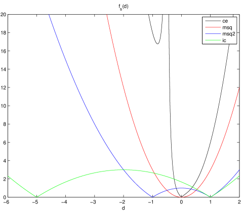
Figure 8.1: Functions $f_{s}$ as in the main text for $s$ equal to $\operatorname{ce}$, $\operatorname{msq}$, $\operatorname{msq}2$, and $\operatorname{ic}$.

Two-stage estimation

In this chapter we shortly discuss a two-stage adaptive method for estimation, in the first stage of which some parameter vector $d$ is computed, with the help of which in the second stage an estimator of the quantity of interest $\alpha\in\mathbb{R}$ is calculated. For a nonempty parameter set $A\in\mathcal{{B}}(\mathbb{R}^{l})$ and a family of distributions as in Section 3.4, let a measurable function $h:\mathcal{{S}}(A)\otimes\mathcal{{S}}_{1}\to\mathcal{{S}}(\overline{\mathbb{R}})$ be such that for each $b\in A$,

$$\mathbb{E}_{\mathbb{Q}(b)}(h(b,\cdot))=\alpha.$$ (9.1)

Let $\operatorname{var}(b)=\operatorname{Var}_{\mathbb{Q}(b)}(h(b,\cdot))$, $b\in A$. Consider some cost variable $C$ and functions $c$ and $\operatorname{ic}$ as in Section 4.1, but in the definition of $\operatorname{ic}$ using the above $\operatorname{var}$ (in particular, for $\operatorname{ic}$ we assume Condition 31). In the IS case conditions 17 and 214 hold, but the above setting is more general and can also describe e.g. control variates or control variates in conjunction with IS. The parameter vector $d$ computed in the first stage is an $A$-valued random variable, which can be obtained e.g. using some adaptive algorithm like single- or multi-stage minimization method of some estimators described in the previous sections. This can be done in many different ways as discussed in the below remark.

Remark 279.

One possibility is to use as $d$ some parameter $d_{t}$ corresponding to some first-stage budget $t$ as in Remark 213. Alternatively, in methods in which to compute some parameter $p_{k}$ one first needs to compute $p_{l}$, $l=1,\ldots,k-1$, like in the MSM methods from the previous sections for $p_{k}$ as in Remark 213, one can set $d=p_{\tau}\mathbb{1}(\tau\neq\infty)+p_{\infty}\mathbb{1}(\tau=\infty)$ for some $p_{\infty}\in A$ and some a.s. finite $\mathbb{N}_{+}\cup\{\infty\}$-valued stopping time $\tau$ for the filtration $\mathcal{{F}}_{n}=\sigma\{p_{l}:l\leq n\}$, $n\in\mathbb{N}_{+}$. For instance, if a.s. $p_{k}\to b^{*}\in A$, then $\tau$ can be the moment when the change of $p_{k}$ from $p_{k-1}$, or such a relative change if $b^{*}\neq 0$, becomes smaller than some $\epsilon\in\mathbb{R}_{+}$ (see e.g. Remark 10 in [43]). For the various $p_{k}$ from MSM methods as in Remark 213, the fact that a.s. $p_{k}\to b^{*}$ follows from Condition 167 or its counterparts. When for some functions $f_{k}:\mathcal{{S}}(A)\otimes(\Omega,\mathcal{{F}})\to\mathcal{{S}}(\mathbb{R})$, $k\in\mathbb{N}_{+}$, (which can be e.g. the minimized estimators) and $f:A\to\mathbb{R}$ we have a.s. $f_{k}(p_{k})\to f(b^{*})$, then such a stopping time can be based on the behaviour of $f_{k}(p_{k})$, similarly as for $p_{k}$ above. Assuming that a.s. $f_{k}\overset{loc}{\rightrightarrows}f$ (see Section 7.3 for sufficient assumptions), if a.s. $p_{k}\to b^{*}$, then from Lemma 191 a.s. $f_{k}(p_{k})\to f(b^{*})$.

One way to model the second stage of a two-stage estimation method is to consider it on a different probability space than the first one, for a fixed computed value $v$ of the variable $d$ from the first stage. In such a case, for some $\kappa_{1},\kappa_{2},\ldots,$ i.i.d. $\sim\mathbb{Q}(v)$, in the second stage we perform an MC procedure as in Chapter 2 but using $Z_{i}=h(v,\kappa_{i})$, $i\in\mathbb{N}_{+}$, e.g. using a fixed number of samples or a fixed approximate budget. We can also construct asymptotic confidence intervals for $\alpha$ as in that chapter. From the discussion in Chapter 2, the inefficiency of such a procedure can be quantified using the inefficiency constant $\operatorname{ic}(v)$. This justifies comparing the asymptotic efficiency of methods for finding the adaptive parameters in the first stage of a two-stage method as above by comparing their first- and, if applicable, second-order asymptotic efficiency for the minimization of $\operatorname{ic}$ as discussed in sections 7.10 and 8.3.

An alternative way to model the second stage of a two-stage method is to consider its second stage on the same probability space as the first one. Let us assume the following condition.

Condition 280.

Random variables $\phi_{i}$, $i\in\mathbb{N}_{+}$, are conditionally independent given $d$ and have the same conditional distribution $\mathbb{Q}(b)$ given $d=b$.

Condition 280 is implied by the following one.

Condition 281.

Condition 19 holds, and for $\beta_{1},\beta_{2},\ldots$, i.i.d. $\sim\mathbb{P}_{1}$ and independent of $d$ we have $(\phi_{i})_{i\in\mathbb{N}_{+}}=(\xi(d,\beta_{i}))_{i\in\mathbb{N}_{+}}$.

In the second stage of the considered method one computes an estimator

$$\widehat{{\alpha}}_{n}=\frac{1}{n}\sum_{i=1}^{n}h(d,\phi_{i}).$$ (9.2)

Similarly as above, the number $n$ of samples can be deterministic or random. In the first case the resulting estimator is unbiased, while in the second this needs not to be true. Random $n$ can correspond e.g. to a fixed approximate computational budget and be given by definition (2.5) or (2.6) but for $C_{i}$ replaced by $C(\phi_{i})$, $i\in\mathbb{N}_{+}$.

Remark 282.

A possible alternative to the above discussed two-stage estimation method is the same as its second model above except that for the computation of $\widehat{{\alpha}}_{n}$ in the second stage one uses the variables $\phi_{i}=\xi(d,\beta_{i})$ as in Condition 281 but without assuming that $\beta_{i}$, $i\in\mathbb{N}_{+}$, are independent of $d$. In such a case, Condition 280 may not hold. For example, one could reuse the i.i.d. random variables with distribution $\mathbb{P}_{1}$ generated for the estimation of $d$ in the first stage as some (potentially all) the variables $\beta_{i}$ used for the computation of $\widehat{{\alpha}}_{n}$, which could save the computation time. Under appropriate identifications, such an approach using exactly the same $\beta_{i}$, $i=1,\ldots,n$ in ESSM to compute $d$ and then (9.2) is used in the multiple control variates method (see [5, 22]), while for IS it was considered in [30]. In such a reusing approach, $\widehat{{\alpha}}_{n}$ as in (9.2) needs not to be unbiased even for $n$ deterministic. Furthermore, one needs to store a potentially large random number of the generated values of random variables, which may be more difficult to implement and requires additional computer memory. Finally, in a number of situations, like in the case of our numerical experiments, generating the required parts of the variables $\beta_{i}$ forms only a small fraction of the computation time needed for computing the variables $h(d,\phi_{i})=(ZL(d))(\xi(d,\beta_{i}))$ in the second stage, so that reusing some $\beta_{i}$ from the first stage would not lead to considerable time savings.

Numerical experiments

Our numerical experiments were carried out using programs written in matlab2012a and run on a laptop. Unless stated otherwise, we used the simulation parameters, variables, and IS basis functions as for the problems of estimation of the expectations $\operatorname{mgf}(x_{0})$, $q_{1,a}(x_{0})$, $q_{2,a}(x_{0})$, and $p_{T,a}(x_{0})$ in Section 5.9. In some of our experiments we performed the single- or multi-stage minimization of estimators $\widehat{{\operatorname{est}}}$ (where for short we write $\widehat{{\operatorname{est}}}$ rather than $\widehat{{\operatorname{est}}}_{n}$, $n\in\mathbb{N}_{p}$, for appropriate $p$) equal to $\widehat{{\operatorname{ce}}}$, $\widehat{{\operatorname{msq}}}$, $\widehat{{\operatorname{msq}2}}$, and $\widehat{{\operatorname{ic}}}$, as discussed in Section 7.1. In the MSM we used in each case $b_{0}=0$. For the minimization of $\widehat{{\operatorname{msq}2}}$ and $\widehat{{\operatorname{ic}}}$ in these methods we used the matlab fminunc unconstrained minimization function with the default settings and exact gradients, for $\widehat{{\operatorname{msq}}}$ additionally using their exact Hessians, as discussed Section 7.1. The minimum points of $\widehat{{\operatorname{ce}}}$ were found by solving the linear systems of equations as in that section. Both for the crude MC (CMC) and when using IS, the computation times of the MC replicates in our experiments were typically approximately proportional to the replicates of the exit times $\tau$ for the MGF and translated committors, and to the replicates of $\tau^{\prime}$ as in (5.73) for $p_{T,a}(x_{0})$. Thus, we consider the theoretical cost variables $C$ equal to $h\tau$ for the MGF and translated committors and to $h\tau^{\prime}$ for $p_{T,a}(x_{0})$. The proportionality constants $p_{\dot{C}}$ of the replicates of such $C$ to the simulation times as in Chapter 2) were different for CMC and when using different basis functions in IS.

The remainder of this chapter is organized as follows. In Section 10.1 we discuss some methods for testing statistical hypotheses, which are later used for interpreting the results of our numerical experiments. In Section 10.2 we describe two-stage estimation experiments as in Section 7.1, performing MSM in the first stages and in the second stages estimating the expectations of the functionals of the Euler scheme as above. In the second stages we also estimated some other quantities, like inefficiency constants, variances, mean costs, and the proportionality constants $p_{\dot{C}}$ as above. We use these quantities to compare the efficiency of applying in a IS MC method the IS parameters obtained from the MSM of different estimators, as well as of using different added constants $a$ and IS basis functions in such adaptive IS procedures. In Section 10.3 we compare the spread of the IS drifts coming from the SSM of different estimators and using different parameters $b^{\prime}$. In Section 10.4 we provide some intuitions behind the results of our numerical experiments.

10.1 Testing statistical hypotheses

Let $\mu_{X},\mu_{Y}\in\mathbb{R}$, $\sigma_{X},\sigma_{Y}\in\mathbb{R}_{+}$, and $\mathbb{R}$-valued random variables $X_{n}$ and $Y_{n}$, $n\in\mathbb{N}_{+}$, be such that $\widetilde{{X}}_{n}:=\sqrt{n}(X_{n}-\mu_{X})\Rightarrow\operatorname{\mathcal{N}}(0,\sigma_{X}^{2})$, $\widetilde{{Y}}_{n}:=\sqrt{n}(Y_{n}-\mu_{Y})\Rightarrow\operatorname{\mathcal{N}}(0,\sigma_{Y}^{2})$, and for each $j,k\in\mathbb{N}_{+}$, $X_{j}$ is independent of $Y_{k}$. Let $\widehat{{\sigma}}_{X,n}$ and $\widehat{{\sigma}}_{Y,n}$, $n\in\mathbb{N}_{+}$, be $[0,\infty)$-valued random variables such that $\widehat{{\sigma}}_{X,n}\overset{p}{\to}\sigma_{X}$ and $\widehat{{\sigma}}_{Y,n}$ $\overset{p}{\to}\sigma_{Y}$. Let $a_{n},b_{n}\in\mathbb{N}_{+}$, $n\in\mathbb{N}_{+}$, be such that $\lim_{n\to\infty}a_{n}=\lim_{n\to\infty}b_{n}=\infty$ and

$$\lim_{n\to\infty}\frac{a_{n}}{b_{n}}=\rho\in\mathbb{R}_{+}.$$ (10.1)

Let

$$t_{n}=\frac{X_{a_{n}}-Y_{b_{n}}}{\sqrt{\frac{\widehat{{\sigma}}_{X,a_{n}}^{2}}{a_{n}}+\frac{\widehat{{\sigma}}_{Y,b_{n}}^{2}}{b_{n}}}}=\frac{\sqrt{a_{n}}(X_{a_{n}}-Y_{b_{n}})}{\sqrt{\widehat{{\sigma}}_{X,a_{n}}^{2}+\frac{a_{n}}{b_{n}}\widehat{{\sigma}}_{Y,b_{n}}^{2}}}\\$$ (10.2)

and $H_{n}=\frac{\sqrt{a_{n}}(\mu_{Y}-\mu_{X})}{\sqrt{\widehat{{\sigma}}_{X,a_{n}}^{2}+\frac{a_{n}}{b_{n}}\widehat{{\sigma}}_{Y,b_{n}}^{2}}}$.

Lemma 283.

Under the assumptions as above, we have

$$t_{n}+H_{n}=\frac{\widetilde{{X}}_{a_{n}}-\sqrt{\frac{a_{n}}{b_{n}}}\widetilde{{Y}}_{b_{n}}}{\sqrt{\widehat{{\sigma}}_{X,a_{n}}^{2}+\frac{a_{n}}{b_{n}}\widehat{{\sigma}}_{Y,b_{n}}^{2}}}\Rightarrow\operatorname{\mathcal{N}}(0,1).$$ (10.3)

Proof.

From the asymptotic properties of $\widetilde{{X}}_{i}$ and $\widetilde{{Y}}_{j}$ as above and their independence, we receive, e.g. using Fubini’s theorem and the fact that convergence in distribution is equivalent to the pointwise convergence of characteristic functions, that

$$\widetilde{{X}}_{a_{n}}-\sqrt{\rho}\widetilde{{Y}}_{b_{n}}\Rightarrow\operatorname{\mathcal{N}}(0,\sigma_{X}^{2}+\rho\sigma_{Y}^{2}).$$ (10.4)

Thus, from $G_{n}:=\widetilde{{Y}}_{b_{n}}(\sqrt{\rho}-\sqrt{\frac{a_{n}}{b_{n}}})\overset{p}{\to}0$,

$$\widetilde{{X}}_{a_{n}}-\sqrt{\frac{a_{n}}{b_{n}}}\widetilde{{Y}}_{b_{n}}=\widetilde{{X}}_{a_{n}}-\sqrt{\rho}\widetilde{{Y}}_{b_{n}}+G_{n}\Rightarrow\operatorname{\mathcal{N}}(0,\sigma_{X}^{2}+\rho\sigma_{Y}^{2}).$$ (10.5)

Furthermore, from the continuous mapping theorem,

$$\sqrt{\widehat{{\sigma}}_{X,a_{n}}^{2}+\widehat{{\sigma}}_{Y,b_{n}}^{2}\frac{a_{n}}{b_{n}}}\overset{p}{\to}\sqrt{\sigma_{X}^{2}+\rho\sigma_{Y}^{2}}.$$ (10.6)

Now, (10.3) follows from (10.5), (10.6), and Slutsky’s lemma. ∎

If $\mu_{X}\leq\mu_{Y}$, then from (10.3) and $H_{n}\geq 0$, $n\in\mathbb{N}_{+}$, for each $\alpha\in(0,1)$ and $z_{1-\alpha}$ as in Remark 7,

$$\limsup_{n\to\infty}\mathbb{P}(t_{n}>z_{1-\alpha})\leq\lim_{n\to\infty}\mathbb{P}(t_{n}+H_{n}>z_{1-\alpha})=\alpha,$$ (10.7)

i.e. the tests of the null hypothesis $\mu_{X}\leq\mu_{Y}$ with the regions of rejection $t_{n}>z_{1-\alpha}$, $n\in\mathbb{N}_{+}$, are pointwise asymptotically level $\alpha$ (see Definition 11.1.1 in [36]). We shall further use such tests for $z_{1-\alpha}=3$, so that $\alpha\approx 0.00270$. If for some selected $n$ we have $t_{n}\geq 3$, i.e. the null hypothesis as above can be rejected, then we shall informally say that the estimate $X_{a_{n}}\pm\frac{\widehat{{\sigma}}_{X,a_{n}}}{\sqrt{a_{n}}}$ of $\mu_{X}$ is (statistically significantly) higher than such an estimate $Y_{b_{n}}\pm\frac{\widehat{{\sigma}}_{Y,b_{n}}}{\sqrt{b_{n}}}$ of $\mu_{Y}$.

Most frequently, for some i.i.d. square integrable random variables $X_{i}^{\prime}$, $i\in\mathbb{N}_{+}$, and such variables $Y_{i}^{\prime}$, $i\in\mathbb{N}_{+}$, independent of $X_{j}^{\prime}$, in such tests we shall use $X_{n}=\frac{1}{n}\sum_{i=1}^{n}X_{i}^{\prime}$ and $\widehat{{\sigma}}_{X,n}=\sqrt{\frac{1}{n-1}\sum_{i=1}^{n}(X_{i}^{\prime}-X_{n})^{2}}$, and analogously for $Y_{n}$ and $\widehat{{\sigma}}_{Y,n}$. In such a case $\frac{\widehat{{\sigma}}_{X,n}}{\sqrt{n}}$ shall be called an estimate of the standard deviation of the mean $X_{n}$.

10.2 Estimation experiments

We first performed $k$-stage minimization methods of the different estimators and for the different estimation problems, using $n_{i}=50\cdot 2^{i-1}$ samples in the $i$th stage for $i=1,\ldots,k$ for various $k\in\mathbb{N}_{+}$ (see Section 7.1). We chose $k=3$ for the problem of estimating $q_{1,a}(x_{0})$, $k=5$ for $\operatorname{mgf}(x_{0})$, and $k=6$ for $p_{T,a}(x_{0})$ and $q_{2,a}(x_{0})$. We first used $a=0.05$ and $M=10$ time-independent IS basis functions as in (5.81). For $i=1,2,\ldots,6$, the IS drifts $r(b_{i})$ corresponding to the minimization results $b_{i}$ from the $i$th stage of the MSM of different estimators for estimating the translated committor $q_{2,a}(x_{0})$ are shown in Figure 10.1. The IS drifts corresponding to the final results of MSM for the estimation of all the expectations are shown in Figure 10.2. In figures 10.1 and 10.2 we also show for comparison approximations of the zero-variance IS drifts $r^{*}$ for the diffusion problems for the translated committors and MGF, computed from formula (5.77) using finite differences instead of derivatives and finite difference approximations of $u$ in that formula computed as in Section 5.9. In Figure 10.1, the IS drifts from the consecutive stages of the MSM of $\widehat{{\operatorname{msq}2}}$ and $\widehat{{\operatorname{ic}}}$ seem to converge the fastest to some limiting drift close to (the approximation of) $r^{*}$, from the MSM of $\widehat{{\operatorname{msq}}}$ — slower, and of $\widehat{{\operatorname{ce}}}$ — the slowest. See Section 10.4 for some intuitions behind these results.

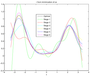
(a)

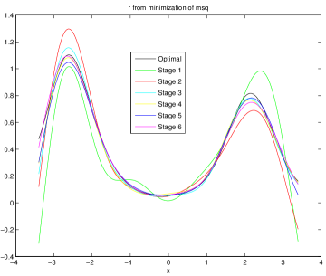
(b)

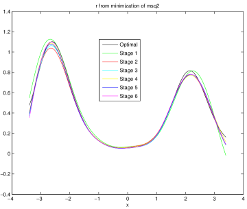
(c)

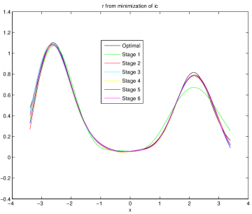
(d)

Figure 10.1: IS drifts from different stages of MSM for estimating $q_{2,a}$, minimizing $\widehat{{\operatorname{ce}}}$ in (a), $\widehat{{\operatorname{msq}}}$ in (b), $\widehat{{\operatorname{msq}2}}$ in (c), and $\widehat{{\operatorname{ic}}}$ in (d). ’Optimal’ denotes an approximation of the zero-variance IS drift $r^{*}$.

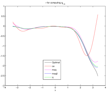
(a)

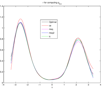
(b)

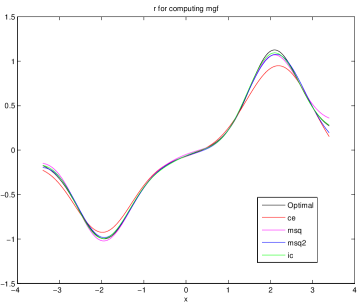
(c)

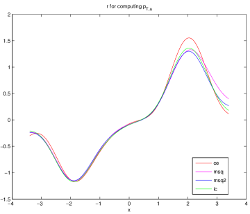
(d)

Figure 10.2: Final IS drifts from the MSM experiments minimizing different estimators, for $q_{1,a}(x_{0})$ in (a), $q_{2,a}(x_{0})$ in (b), $\operatorname{mgf}(x_{0})$ in (c), and $p_{T,a}(x_{0})$ in (d). “Optimal“ denotes an approximation of the zero-variance IS drift.

Consider a numerical experiment in which, for a given IS parameter $v\in A$, we compute unbiased estimates of the mean cost $c(v)$ as well as of the variance $\operatorname{var}(v)$ and the (theoretical) inefficiency constant $\operatorname{ic}(v)$ of the IS estimator of the expectation of the functional of the Euler scheme of interest, using estimators (4.28), (4.31), and (4.23) respectively for $b=b^{\prime}=v$ and $n=10$. For some $\beta_{1},\ldots,\beta_{n}$ i.i.d. $\sim\mathbb{U}$, these estimators are evaluated on $(\xi(\beta_{i},v))_{i=1}^{n}$ (for $\xi$ as in (5.35)), so that the computations involve simulating $n$ independent Euler schemes with an additional drift $r(v)$ as in (5.57). Such experiments for the different estimation problems and for $v$ equal to the final results of the MSM of $\widehat{{\operatorname{ce}}}$, $\widehat{{\operatorname{msq}}}$, $\widehat{{\operatorname{msq}2}}$, and $\widehat{{\operatorname{ic}}}$ as above, and for $v=0$ for CMC, were repeated independently $K$ times in an outer MC loop for different $K$. For the problem of the estimation of $q_{2,a}(x_{0})$ we additionally used as $v$ the minimization result from the third step of MSM. For the MGF we made in all the cases $K=75000$ repetitions. For the translated committors, when using CMC or IS with a parameter $v$ from the $3$-stage MSM of estimators other than $\widehat{{\operatorname{ce}}}$, we took $K=2000$, while in the other cases we chose $K=5000$. For $p_{T,a}$ we made $K=20000$ repetitions both for the CMC and when using $v$ from the MSM of $\widehat{{\operatorname{ce}}}$, and $K=2\cdot 10^{5}$ repetitions for $v$ from the MSM of $\widehat{{\operatorname{msq}}}$, $\widehat{{\operatorname{msq}2}}$, and $\widehat{{\operatorname{ic}}}$. The MC means of the inefficiency constant and variance estimators from the outer loops for the translated committors and MGF are given in Table 10.1, along with the estimates of the standard deviations of such means. For $p_{T,a}(x_{0})$, such outer MC loop estimates of the inefficiency constants, variances, and mean costs are given in Table 10.2.

	CMC	$\widehat{{\operatorname{ce}}}$	$\widehat{{\operatorname{msq}}}$	$\widehat{{\operatorname{msq}2}}$	$\widehat{{\operatorname{ic}}}$
	Estimates of inefficiency constants ($\cdot 10^{-3}$)
$q_{1,a}$	$7204\pm 92$	$4855\pm 649$	$507\pm 10$	$129.1\pm 3.8$	$132.9\pm 3.5$
$q_{2,a}$, $k=3$	$7300\pm 88$	$553\pm 26$	$60.8\pm 1.2$	$53.4\pm 1.0$	$50.5\pm 1.1$
$q_{2,a}$ , $k=6$		$73.1\pm 1.0$	$56.10\pm 0.69$	$48.78\pm 0.59$	$47.99\pm 0.61$
$\operatorname{mgf}$	$2041\pm 15$	$6.276\pm 0.055$	$3.691\pm 0.035$	$3.177\pm 0.029$	$3.163\pm 0.028$
	Estimates of variances $(\cdot 10^{-3})$
$q_{1,a}$	$174.0\pm 1.7$	$126\pm 14$	$12.36\pm 0.20$	$3.155\pm 0.083$	$3.208\pm 0.073$
$q_{2,a}$, $k=3$	$177.43\pm 1.7$	$16.35\pm 0.79$	$1.437\pm 0.021$	$1.268\pm 0.019$	$1.223\pm 0.020$
$q_{2,a}$, $k=6$		$1.794\pm 0.021$	$1.347\pm 0.013$	$1.164\pm 0.011$	$1.169\pm 0.012$
$\operatorname{mgf}$	$49.41\pm 0.32$	$0.9040\pm 0.0072$	$0.3732\pm 0.0029$	$0.3195\pm 0.0024$	$0.3209\pm 0.0024$

Table 10.1: Estimates of the inefficiency constants and variances of the estimators of the translated committors for $a=0.05$ and the MGF when using CMC or IS with IS parameters from the MSM of different estimators. For $q_{2,a}$ we consider using the IS parameters from the $k$th stages of MSM for $k\in\{3,6\}$.

	CMC	$\widehat{{\operatorname{ce}}}$	$\widehat{{\operatorname{msq}}}$	$\widehat{{\operatorname{msq}2}}$	$\widehat{{\operatorname{ic}}}$
$\operatorname{ic}\ (\cdot 10^{-3})$	$1391\pm 5$	$65.22\pm 0.30$	$63.332\pm 0.09$	$62.677\pm 0.090$	$61.863\pm 0.091$
$\operatorname{var}\ (\cdot 10^{-3})$	$150.78\pm 0.58$	$10.258\pm 0.042$	$10.036\pm 0.013$	$9.8937\pm 0.0126$	$9.9491\pm 0.0130$
$c$	$9.227\pm 0.004$	$6.3608\pm 0.0066$	$6.3117\pm 0.0021$	$6.3355\pm 0.0021$	$6.2173\pm 0.0021$

Table 10.2: Estimates of the inefficiency constants and variances of the estimators of $p_{T,a}$ for $a=0.05$ as well as of the mean costs, when using CMC or IS with the IS parameters from the MSM of different estimators.

Remark 284.

Note that due to Remark 64, the variables $C$ as above have all moments (and thus also variance) finite under $\mathbb{Q}(v)$, $v\in A$. For $v=0$ (i.e. for CMC), from the boundedness of the considered $Z$, we have the finiteness of the mean costs and of the variances and inefficiency constants of the estimators of the Euler scheme expectations of interest as well as of the variances of the utilized estimators of such quantities. For the general $v$ and bounded stopping times (as is the case for such times equal to $\tau^{\prime}$ as in (5.73) when estimating $p_{T,a}$), the finiteness of the quantities as in the previous sentence follows from the corresponding $Z$ being bounded, as well as from Theorem 121 and Remark 119. In cases when the stopping time is not bounded (like for such a time equal to $\tau$ for the MGF and translated committors as above), one can ensure such boundedness by terminating the simulations at some fixed time as discussed in Section 6.2. We did not terminate our simulations, but still our results can be interpreted as coming from simulations terminated at some time larger than any of the exit times encountered in our experiments.

From tables 10.1 and 10.2 we can see that using the IS parameters from the MSM of $\widehat{{\operatorname{ic}}}$ and $\widehat{{\operatorname{msq}2}}$ led in each case to the lowest estimates of variances and (theoretical) inefficiency constants, followed by the ones from using the parameters from the MSM of $\widehat{{\operatorname{msq}}}$, and finally $\widehat{{\operatorname{ce}}}$. Using CMC led in each case to the highest such estimates. For $q_{2,a}(x_{0})$ and each of $\widehat{{\operatorname{ce}}}$, $\widehat{{\operatorname{msq}}}$, and $\widehat{{\operatorname{msq}2}}$, using the IS parameter from the sixth stage of MSM led to a lower estimate of variance and inefficiency constant than using such a parameter from the third stage. Note also that the estimates of the inefficiency constants and variances for $q_{2,a}(x_{0})$ when using the IS parameters from the third stage of the MSM of $\widehat{{\operatorname{msq}2}}$ and $\widehat{{\operatorname{ic}}}$ are lower than when using the parameters from the sixth stage of the MSM of $\widehat{{\operatorname{ce}}}$ and $\widehat{{\operatorname{msq}}}$ (though for the estimates of the inefficiency constants for $\widehat{{\operatorname{msq}2}}$ and $\widehat{{\operatorname{msq}}}$ we cannot confirm this at the desired significance level as in Section 10.1). For $p_{T,a}(x_{0})$, the estimate of the inefficiency constant, variance, and mean cost is respectively lower, higher, and lower when minimizing $\widehat{{\operatorname{ic}}}$ than $\widehat{{\operatorname{msq}2}}$. Some intuitions behind these results are given by Theorem 209 and Remark 129, see also the discussion in Section 10.4.

Using the IS parameters $v$ from the MSM of $\widehat{{\operatorname{ic}}}$ as above and averaging the estimates from the $nK$ simulations available in each case we computed the IS MC estimates of the quantities of interest: $\operatorname{mgf}(x_{0})$, and using the translated estimators as in Section 5.7 also of $p_{T}(x_{0})$ and $q_{i}(x_{0})$, $i=1,2$. The results are presented in Table 10.3. Note that we have $q_{1}(x_{0})=1-q_{2}(x_{0})\approx 0.78$ and the estimates of the inefficiency constants in Table 10.1 for estimating the lower value committor $q_{2}(x_{0})$ are lower. Thus, it seems reasonable to use the translated IS estimator for $q_{2}(x_{0})$ also for computing $q_{1}(x_{0})$ as discussed in Section 5.7.

$q_{1}(x_{0})$	$q_{2}(x_{0})$	$\operatorname{mgf}(x_{0})$	$p_{T}(x_{0})$
$0.7751\pm 0.0004$	$0.22597\pm 0.00025$	$0.16682\pm(6\cdot 10^{-5})$	$0.18396\pm(7\cdot 10^{-5})$

Table 10.3: Estimates of different expectations obtained from IS MC using IS parameters from the MSM of $\widehat{{\operatorname{ic}}}$.

In the above experiments utilising $nK$ simulations we also computed the MC estimates of the mean costs $c(v)$. For comparison we also computed an estimate of the mean cost in CMC (equal to $c(0)=\mathbb{E}_{\mathbb{U}}(\tau)$), using an MC average of such costs from $7.5\cdot 10^{5}$ simulations. The results are provided in Table 10.4. Note that the estimates of the mean costs in tables 10.2 and 10.3 are lower for IS using the IS parameters $v$ from the MSM methods for computing $\operatorname{mgf}(x_{0})$ and $p_{T,a}(x_{0})$ than for the respective CMC methods. As discussed in Section 3.3, an intuition behind these results is provided by Theorem 16.

	$q_{1,a}(x_{0})$	$q_{2,a}(x_{0})$	$\operatorname{mgf}(x_{0})$	CMC
$c$	$41.26\pm 0.28$	$41.18\pm 0.28$	$9.89\pm 0.03$	$41.44\pm 0.15$

Table 10.4: Estimates of the mean costs when using the IS parameters from the MSM of $\widehat{{\operatorname{ic}}}$ and for CMC, for the problems of computing the translated committors for $a=0.05$ and MGF.

We also performed two-stage experiments similar as above for $q_{2,a}(x_{0})$ and $p_{T,a}(x_{0})$ for several different added constants $a\in\mathbb{R}_{+}$ other than $a=0.05$ considered above. For $q_{2,a}(x_{0})$ we used the IS basis functions as above, while for $p_{T,a}(x_{0})$ also the time-dependent basis functions as in (5.82) for $M=5$ and $M=10$ and various $p\in\mathbb{N}_{+}$. This time in the first stages we performed the MSM only of $\widehat{{\operatorname{ic}}}$ for $k=3$ and $n_{i}=400\cdot 2^{i-1}$, $i=1,\ldots,k$, so that the number of samples $n_{k}=1600$ used in the final stages of MSM was the same as for $a=0.05$ above. In the second stages we estimated the inefficiency constants, mean costs, and variances in an external loop like above. For $q_{2,a}(x_{0})$ we made $K=3000$ repetitions in such a loop, while for $p_{T,a}(x_{0})$ — $K=10000$ for the basis functions as in (5.81), as well as $K=50000$ for the basis functions as in (5.82) for $M=5$ and $K=30000$ for $M=10$. The results are presented in tables 10.5, 10.6, and 10.7, along with the results for the case of $a=0.05$ considered before. The smallest estimates of the inefficiency constants and variances for $q_{2,a}(x_{0})$ were obtained for $a=0.05$. For $p_{T,a}(x_{0})$ and the basis functions as in (5.81), we obtained the smallest variance for $a=0.2$ and the lowest inefficiency constants for $a=0.1$ and $a=0.2$. Among all the cases for $p_{T,a}$, the smallest variances and theoretical inefficiency constants were received for $a=0$ and when using the time-dependent IS basis functions (5.82) for $M=10$ and $p=3$.

$a=$	$0$	$0.05$	$0.1$	$0.2$
$\operatorname{ic}\ (\cdot 10^{-3})$	$82.6\pm 2.3$	$47.99\pm 0.61$	$51.89\pm 0.80$	$55.52\pm 0.86$
$\operatorname{var}\ (\cdot 10^{-3})$	$2.008\pm 0.058$	$1.169\pm 0.012$	$1.252\pm 0.016$	$1.359\pm 0.016$

Table 10.5: Estimates of the inefficiency constants and variances of the IS estimators of $q_{2,a}$ for different $a$, corresponding to IS with the parameters from the MSM of $\widehat{{\operatorname{ic}}}$.

$a=$	$0$	$0.05$	$0.1$	$0.2$	$0.3$
$\operatorname{ic}\ (\cdot 10^{-3})$	$100.8\pm 0.7$	$61.86\pm 0.09$	$55.95\pm 0.35$	$56.44\pm 0.39$	$61.43\pm 0.48$
$\operatorname{var}\ (\cdot 10^{-3})$	$17.88\pm 0.10$	$9.949\pm 0.013$	$8.224\pm 0.047$	$7.544\pm 0.050$	$7.794\pm 0.058$
$c$	$5.641\pm 0.009$	$6.2173\pm 0.0021$	$6.803\pm 0.009$	$7.489\pm 0.009$	$7.874\pm 0.009$

Table 10.6: Estimates of the inefficiency constants and variances of the estimators of $p_{T,a}$ for different $a$, and estimates of the mean costs, corresponding to IS with the parameters from the MSM of $\widehat{{\operatorname{ic}}}$ and using $M=10$ time-independent IS basis functions as in (5.81).

	$M=5$				$M=10,\ a=0$
	$p=1,\ a=0$	$p=1,\ a=0.05$	$p=2,\ a=0$	$p=3,\ a=0$	$p=1$	$p=2$	$p=3$
$\operatorname{ic}\ (\cdot 10^{-3})$	$63.01\pm 0.39$	$93.44\pm 0.45$	$48.18\pm 0.28$	$46.52\pm 0.23$	$34.11\pm 0.16$	$22.95\pm 0.17$	$17.34\pm 0.12$
$\operatorname{var}\ (\cdot 10^{-3})$	$10.544\pm 0.064$	$13.60\pm 0.06$	$7.975\pm 0.045$	$7.629\pm 0.036$	$5.714\pm 0.025$	$3.899\pm 0.027$	$2.951\pm 0.019$
$c$	$5.978\pm 0.003$	$6.871\pm 0.004$	$6.037\pm 0.003$	$6.086\pm 0.003$	$5.966\pm 0.004$	$5.878\pm 0.004$	$5.887\pm 0.004$

Table 10.7: Estimates of the inefficiency constants and variances of IS estimators of $p_{T,a}$ for different $a$, as well as of the mean costs, corresponding to IS with the parameters from the MSM of $\widehat{{\operatorname{ic}}}$, using the time-dependent IS basis functions as in (5.82) for different $M$ and $p$.

In our experiments, when using CMC and IS MC with different sets of IS basis functions, the proportionality constants $p_{\dot{C}}$ as in Chapter 2 were considerably different. Thus, to compare the efficiency of the MC methods using estimators corresponding to these different bases, one should compare their practical rather than theoretical inefficiency constants. We performed separate experiments approximating some $p_{\dot{C}}$ as above and computing the corresponding practical inefficiency constants (equal to the products of such $p_{\dot{C}}$ and the respective theoretical inefficiency constants). For $n=10^{5}$, we ran $n$-step CMC and IS MC procedures for estimating $q_{2,0.05}(x_{0})$ using the IS basis functions as in (5.81), and for estimating $p_{T,a}$: for $a=0.05$ for IS basis functions as in (5.81) for $M=10$, and for $a=0$ for IS basis functions as in (5.82): for $M=5$ and $p=1$, and for $M=10$ and $p\in\{1,3\}$. When performing the IS MC we used the IS parameters from the final stages of the corresponding MSM procedures as above. For $C_{i}$ being the theoretical cost of the $i$th step of a given MC procedure and $\dot{C}_{i}$ being its practical cost equal to its computation time calculated using the matlab tic and toc functions, as an approximation of $p_{\dot{C}}$ we used the ratio $\widehat{{p}}_{\dot{C},n}=\frac{\sum_{i=1}^{n}\dot{C}_{i}}{\sum_{i=1}^{n}C_{i}}$. Treating $(\dot{C}_{i},C_{i})$, $i=1,2,\ldots,$ as i.i.d. random vectors with square-integrable coordinates, for $p_{\dot{C}}:=\frac{\mathbb{E}(\dot{C}_{1})}{\mathbb{E}(C_{1})}$, from the delta method it easily follows that for

$$\sigma:=p_{\dot{C}}\sqrt{\frac{\operatorname{Var}(C_{1})}{(\mathbb{E}(C_{1}))^{2}}+\frac{\operatorname{Var}(\dot{C_{1}})}{(\mathbb{E}(\dot{C}_{1}))^{2}}-2\frac{\operatorname{Cov}(C_{1},\dot{C_{1}})}{\mathbb{E}(\dot{C}_{1})\mathbb{E}(C_{1})}}$$ (10.8)

we have $\sqrt{n}(\widehat{{p}}_{\dot{C},n}-p_{\dot{C}})\Rightarrow\operatorname{\mathcal{N}}(0,\sigma^{2})$. For $\widehat{{\sigma}}_{n}$ being an estimate of $\sigma$ in which instead of means, variances, and covariances one uses their standard unbiased estimators computed using $(C_{i},\dot{C}_{i})_{i=1}^{n}$, we have a.s. $\frac{\widehat{{\sigma}}_{n}}{\sigma}\to 1$. Thus, from Slutsky’s lemma, $\frac{\sqrt{n}}{\widehat{{\sigma}}_{n}}(\widehat{{p}}_{\dot{C},n}-p_{\dot{C}})\Rightarrow\operatorname{\mathcal{N}}(0,1)$, which can be used for constructing asymptotic confidence intervals for $p_{\dot{C}}$. In Table 10.8 we provide the computed estimates in form $\widehat{{p}}_{\dot{C},n}\pm\frac{\widehat{{\sigma}}_{n}}{\sqrt{n}}$. It can be seen that these approximations of $p_{\dot{C}}$ are close for $q_{2,a}(x_{0})$ and $p_{T,a}(x_{0})$ when using in both cases CMC or IS with the basis functions as in (5.81), and for $p_{T,a}(x_{0})$ when using the basis functions as in (5.82) for $M=10$ and different $p$. However, such $p_{\dot{C}}$ differ significantly for the other pairs of MC methods. In Table 10.8 we also provide the estimates of practical inefficiency constants $\dot{\operatorname{ic}}$ obtained by multiplying the corresponding estimates of the theoretical inefficiency constants computed earlier by the received approximations of $p_{\dot{C}}$. From this table we can see that using IS in the considered cases led to considerable practical inefficiency constant reductions over using CMC.

	$q_{2,a}$		$p_{T,a}$
	CMC	$M=10$	CMC	$M=10$	$M=5$, $p=1$	$M=10$, $p=1$	$M=10$, $p=3$
$p_{\dot{C}}$ ($\cdot 10^{-6}$s)	$33.612\pm 0.003$	$137.06\pm 0.01$	$33.998\pm 0.004$	$138.75\pm 0.01$	$96.36\pm 0.01$	$148.92\pm 0.01$	$149.74\pm 0.01$
$\dot{\operatorname{ic}}$ ($\cdot 10^{-3}s$)	$245.4\pm 3.0$	$6.578\pm 0.084$	$47.3\pm 0.2$	$8.584\pm 0.013$	$6.072\pm 0.038$	$5.080\pm 0.024$	$2.597\pm 0.018$

Table 10.8: Estimates of $p_{\dot{C}}$ and $\dot{\operatorname{ic}}$ for computing $q_{2,a}$ and $p_{T,a}$ for various $a$ and IS basis functions as discussed in the main text.

10.3 Experiments comparing the spread of IS drifts.

In the experiments described in this section we consider the assumptions as for the estimation of $q_{2,a}(x_{0})$ in Section 5.9. For the estimators $\widehat{{\operatorname{est}}}$ equal to each of $\widehat{{\operatorname{ce}}}$, $\widehat{{\operatorname{msq}}}$, $\widehat{{\operatorname{msq}2}}$, and $\widehat{{\operatorname{ic}}}$, we performed $20$ independent SSM experiments for $n_{1}=100$ and $b^{\prime}=0$ as in Section 7.1, i.e. minimizing $b\to\widehat{{\operatorname{est}}}_{n_{1}}(b^{\prime},b)(\widetilde{{\chi}}_{1})$ for some $\widetilde{{\chi}}_{1}$ as in that section. For each such experiment for $\widehat{{\operatorname{est}}}=\widehat{{\operatorname{ic}}}$, for the same $\widetilde{{\chi}}_{1}$ as in that experiment, we additionally carried out a two-phase minimization, in its first phase minimizing $b\to\widehat{{\operatorname{msq}}}_{n}(b^{\prime},b)(\widetilde{{\chi}}_{1})$ and in the second $b\to\widehat{{\operatorname{ic}}}_{n}(b^{\prime},b)(\widetilde{{\chi}}_{1})$, using the first-phase minimization result as a starting point. The IS drifts corresponding to the IS parameters computed in the above experiments are shown in Figure 10.3, in which we also show an approximation of the zero-variance IS drift $r^{*}$ for the corresponding diffusion problem as in the previous section.

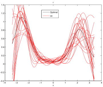
(a)

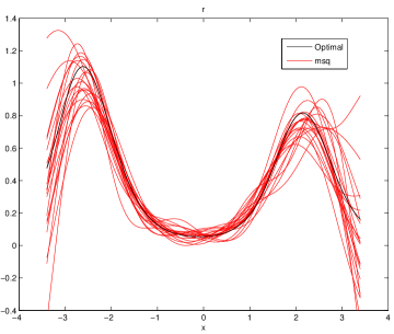
(b)

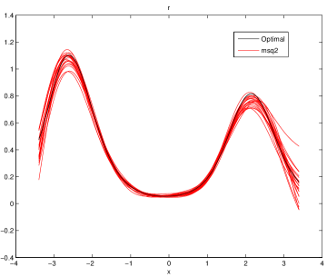
(c)

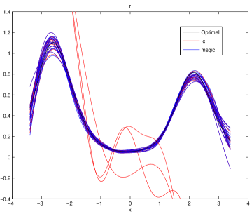
(d)

Figure 10.3: The IS drifts from SSM for estimating $q_{2,a}$, minimizing $\widehat{{\operatorname{ce}}}$ in (a), $\widehat{{\operatorname{msq}}}$ in (b), $\widehat{{\operatorname{msq}2}}$ in (c), and $\widehat{{\operatorname{ic}}}$ in (d). The ”optimal“ IS drift is a finite-difference approximation of the zero-variance IS drift $r^{*}$. The label ’msqic’ in (d) corresponds to the two-phase minimization and ’ic’ to the single-phase minimization as discussed in the main text.

From Figure 10.3 (d) it can be seen that ordinary (i.e. single-phase) SSM using $\widehat{{\operatorname{ic}}}$ yielded in three experiments IS drifts far from $r^{*}$, while in the other $17$ experiments and in all $20$ experiments when using two-phase minimization we received drifts close to $r^{*}$. In the experiments in which ordinary minimization led to drifts far from $r^{*}$, the value of $\widehat{{\operatorname{ic}}}_{n}(b^{\prime},b)(\widetilde{{\chi}}_{1})$ in the minimization result $b$ was several times smaller than when using two-phase minimization, while in the other cases these values were very close (e.g. the absolute value of difference of such values divided by the smaller of them was in each case below $1\%$). In Figure 10.3, the IS drifts from the SSM of $\widehat{{\operatorname{msq}2}}$ and the two-phase minimization minimizing $\widehat{{\operatorname{ic}}}$ in the second phase as above seem to be the least spread, followed by the ones from the minimization of $\widehat{{\operatorname{msq}}}$, and finally $\widehat{{\operatorname{ce}}}$.

From the below remark it can be expected that for a sufficiently large $n$, the IS drifts from SSM experiments like above should have approximately normal distribution in each point.

Remark 285.

Let $A$, $T$, $d_{t}$, and $r_{t}$ be as in Section 8.1 and let for some covariance matrix $D\in\mathbb{R}^{l\times l}$ it hold

$$\sqrt{r_{t}}(d_{t}-b^{*})\Rightarrow\operatorname{\mathcal{N}}(0,D).$$ (10.9)

This holds e.g. for $d_{t}$ being the SSM or MSM results of the estimators $\widehat{{g}}$ for $g$ replaced by $\operatorname{ce}$, $\operatorname{msq}$, $\operatorname{msq}2$, or $\operatorname{ic}$, for the SSM under the assumptions as in Section 8.5 for $D=u(b^{\prime})V_{g}(b^{\prime})$ and $r_{t}=t$, $t\in T$, while for the MSM under the assumptions as in Section 8.7 for $D=V_{g}(d^{*})$, $T=\mathbb{N}_{+}$, and $r_{k}=n_{k}$, $k\in T$. Let us assume a linear parametrization of the IS drifts as in (5.58), let $x\in\mathbb{R}^{m}$, and let $B\in\mathbb{R}^{l\times d}$ be such that $B_{i,j}=(\widetilde{{r}}_{i})_{j}(x)$, $i=1,\ldots,l$, $j=1\ldots,d$. Then, $r(d_{t})(x)=B^{T}d_{t}$, $t\in T$, and from (10.9)

$$\sqrt{r_{t}}(r(d_{t})-r(b^{*}))(x)\Rightarrow\operatorname{\mathcal{N}}(0,B^{T}DB).$$ (10.10)

In the further experiments, to be able to carry out more simulations in a reasonable time, we changed the model considered by increasing the temperature $10$ times. For such a new temperature we received an estimate $1.468\pm 0.002$ of the mean cost $h\mathbb{E}_{\mathbb{U}}(\tau)$ in CMC, as compared to $41.44\pm 0.15$ under the original temperature as in Table 10.3. We carried out an MSM procedure of $\widehat{{\operatorname{msq}2}}$ for $k=6$ and $n_{i}=50\cdot 2^{i-1}$, $i=1,\ldots,k$, receiving the final minimization result $b_{MSM}$. For $\widehat{{\operatorname{est}}}$ equal to each of the different estimators as above and for $b^{\prime}=0$ and $b^{\prime}=b_{MSM}$, we carried out independently $N=5000$ times the SSM of $\widehat{{\operatorname{est}}}$ for $n_{1}=200$, in the $i$th SSM receiving a result $a_{i}$ and then computing $r(a_{i})(0)$, i.e. the corresponding IS drift at zero, $i=1,\ldots,N$. The histograms of such IS drifts at zero for $b^{\prime}=0$, with fitted Gaussian functions, are shown in Figure 10.4.

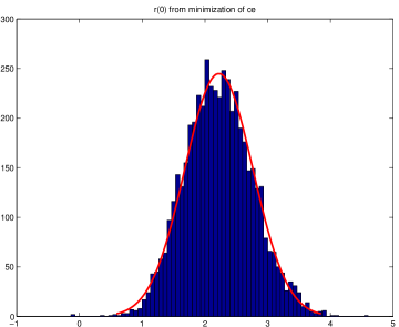
(a)

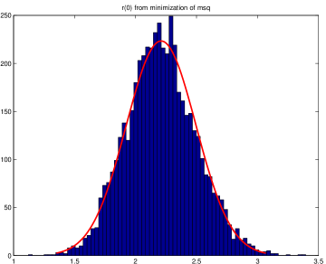
(b)

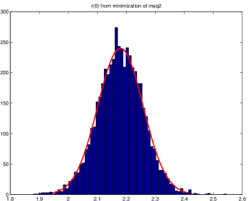
(c)

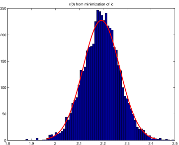
(d)

Figure 10.4: Histograms of the IS drifts at zero from the SSM for computing $q_{2,a}$, minimizing $\widehat{{\operatorname{ce}}}$ in (a), $\widehat{{\operatorname{msq}}}$ in (b), $\widehat{{\operatorname{msq}2}}$ in (c), and $\widehat{{\operatorname{ic}}}$ in (d).

This figure suggests that the distributions of the IS drifts at zero are approximately normal, as could be expected from Remark 285. Furthermore, the (empirical) distribution of the IS drifts at zero for $b^{\prime}=0$ seems to be in a sense the least spread when minimizing $\widehat{{\operatorname{msq}2}}$ and $\widehat{{\operatorname{ic}}}$, followed by $\widehat{{\operatorname{msq}}}$, and finally $\widehat{{\operatorname{ce}}}$. The same observations can be made from the inspection of histograms for the case of $b^{\prime}=b_{MSM}$, which are not shown. We shall now compare quantitatively the spread of empirical distributions of the IS drifts at zero in the above experiments for the different estimators and $b^{\prime}$ used, using interquartile ranges (IQRs), the definition and some required properties of which are provided in the below remark.

Remark 286.

For i.i.d. random variables $X_{1},X_{2},\ldots$, and $k,n\in\mathbb{N}_{+}$, let $X_{k:n}$ be the $k$th coordinate of $\widetilde{{X}}_{n}:=(X_{i})_{i=1}^{n}$ in the nondecreasing order. For $n\geq 4$, let us define the interquartile range (IQR) of the coordinates of $\widetilde{{X}}_{n}$ as $\widehat{{\operatorname{IQR}}}_{n}=X_{\lfloor\frac{3n}{4}\rfloor:n}-X_{\lfloor\frac{n}{4}\rfloor:n}$. Let further $X_{1}\sim\operatorname{\mathcal{N}}(\mu,\sigma^{2})$ for some $\mu\in\mathbb{R}$ and $\sigma\in\mathbb{R}_{+}$, and let $q$ denote the IQR of $\operatorname{\mathcal{N}}(\mu,\sigma^{2})$ (i.e. the difference of its third and first quartile). Then, for a certain $d\approx 1.36$ we have $\sqrt{n}(\widehat{{\operatorname{IQR}}}_{n}-q)\Rightarrow\operatorname{\mathcal{N}}(0,dq^{2})$ (see page 327 in [15]). Thus, for $\widehat{{\sigma}}_{n}=\sqrt{d}\widehat{{\operatorname{IQR}}}_{n}$ we have $\frac{\sqrt{n}}{\widehat{{\sigma}}_{n}}(\widehat{{\operatorname{IQR}}}_{n}-q)\Rightarrow\operatorname{\mathcal{N}}(0,1)$, which can be used for constructing asymptotic confidence intervals for $q$. For some $\mu^{\prime}\in\mathbb{R}$ and $\sigma^{\prime}\in\mathbb{R}_{+}$, consider further $X_{1}^{\prime},X_{2}^{\prime}\ldots,$ i.i.d. $\sim\operatorname{\mathcal{N}}(\mu^{\prime},(\sigma^{\prime})^{2})$, such that $(X_{i}^{\prime})_{i\in\mathbb{N}_{+}}$ is independent of $(X_{i})_{i\in\mathbb{N}_{+}}$, and let $q^{\prime}\in\mathbb{R}_{+}$ be the IQR of $\operatorname{\mathcal{N}}(\mu^{\prime},(\sigma^{\prime})^{2})$. Then, for $\widehat{{\operatorname{IQR}}}_{n}^{\prime}$ analogous as above but for the primed variables we have $(\widehat{{\operatorname{IQR}}}_{n}-q,\widehat{{\operatorname{IQR}}}_{n}^{\prime}-q^{\prime})\Rightarrow\operatorname{\mathcal{N}}(0,d\operatorname{diag}(q^{2},(q^{\prime})^{2}))$. Thus, for $R=\frac{q}{q^{\prime}}$, $\widehat{{R}}_{n}=\frac{\widehat{{\operatorname{IQR}}}_{n}}{\widehat{{\operatorname{IQR}}}_{n}^{\prime}}$, and $\sigma_{R}=R\sqrt{2d}$, from the delta method we have $\sqrt{n}(\widehat{{R}}_{n}-R)\Rightarrow\operatorname{\mathcal{N}}(0,\sigma_{R}^{2})$. Therefore, for $\widehat{{\sigma}}_{R,n}=\widehat{{R}}_{n}\sqrt{2d}$ we have $\frac{\sqrt{n}}{\widehat{{\sigma}}_{R,n}}(\widehat{{R}}_{n}-R)\Rightarrow\operatorname{\mathcal{N}}(0,1)$.

For $X_{i}=r(a_{i})(0)$, $i=1,\ldots,N$, received from the SSM of different estimators as above, we computed the estimates $\widehat{{\operatorname{IQR}}}_{N}$ of the IQRs of drifts at zero and the values $\frac{\widehat{{\sigma}}_{N}}{\sqrt{N}}$ as in Remark 286. The results are provided in Table 10.9.

	$\widehat{{\operatorname{ce}}}$	$\widehat{{\operatorname{msq}}}$	$\widehat{{\operatorname{msq}2}}$	$\widehat{{\operatorname{ic}}}$
$b^{\prime}=0$	$0.736\pm 0.012$	$0.3770\pm 0.0062$	$0.1039\pm 0.0017$	$0.1006\pm 0.0017$
$b^{\prime}=b_{MSM}$	$0.546\pm 0.009$	$0.2910\pm 0.0048$	$0.0932\pm 0.0015$	$0.0929\pm 0.0015$

Table 10.9: Estimates of the IQRs of the IS drifts at zero and the values $\frac{\widehat{{\sigma}}_{N}}{\sqrt{N}}$ from the SSM of various estimators.

From this table we can see that for the both values of $b^{\prime}$ the computed estimates of IQRs from the minimization of $\widehat{{\operatorname{ic}}}$ and $\widehat{{\operatorname{msq}2}}$ are the lowest, followed by such estimates from the minimization of $\widehat{{\operatorname{msq}}}$, and finally $\widehat{{\operatorname{ce}}}$. The ratio of the estimates of IQRs from the minimization of $\widehat{{\operatorname{ce}}}$ to $\widehat{{\operatorname{msq}}}$ is $1.951\pm 0.045$ for $b^{\prime}=0$ and $1.8771\pm 0.044$ for $b^{\prime}=b_{MSM}$ (where the results are provided in the form $\widehat{{R}}_{n}\pm\frac{\widehat{{\sigma}}_{R,N}}{\sqrt{N}}$ under appropriate identifications with the variables from Remark 286). Note that these ratios are close to $2$. Intuitions supporting the above results are given in Section 10.4. Note also that the estimates of IQRs are lower when using $b^{\prime}=b_{MSM}$ than $b^{\prime}=0$.

10.4 Some intuitions behind certain results of our numerical experiments

Recall that in the numerical experiments in Section 10.2 we observed the fastest convergence of the IS drifts in the MSM results and in Section 10.3 the lowest spreads of such drifts in the SSM results when minimizing $\widehat{{\operatorname{msq}2}}$ and $\widehat{{\operatorname{ic}}}$, followed by $\widehat{{\operatorname{msq}}}$, and finally $\widehat{{\operatorname{ce}}}$. Furthermore, in Section 10.3 the IQRs of the values at zero of the IS drifts corresponding to the SSM results were approximately two times higher when minimizing $\widehat{{\operatorname{ce}}}$ than $\widehat{{\operatorname{msq}}}$. In this section we provide some intuitions behind these and some other of our experimental results. We will need the following remark.

Remark 287.

Let us assume that, similarly as in Section 8.9, for $b^{*}$ being a zero-variance IS parameter, for each $b\in\mathbb{R}^{l}$ we have $V_{\operatorname{msq}2}(b)=V_{\operatorname{ic}}(b)=0$, $V_{\operatorname{ce}}(b)=4V_{\operatorname{msq}}(b)$, and $V_{\operatorname{ce}}(b)$ is positive definite. Let further, similarly as in Remark 285, for $d=1$, for $g$ replaced by each of $\operatorname{ce}$, $\operatorname{msq}$, $\operatorname{msq}2$, and $\operatorname{ic}$, for $x\in\mathbb{R}^{m}$ and $B=((\widetilde{{r}}_{i})(x))_{i=1}^{l}$, for $u(b^{\prime})\in\mathbb{R}_{+}$, $r_{t}=t$, and $v_{g}=u(b^{\prime})B^{T}V_{g}(b^{\prime})B$ for SSM or $r_{k}=n_{k}$ and $v_{g}=B^{T}V_{g}(d^{*})B$ for MSM, the IS drifts corresponding to the SSM or MSM results $d_{t}$ of the estimators $\widehat{{g}}$ respectively fulfill

$$\sqrt{r_{t}}(r(d_{t})-r(b^{*}))(x)\Rightarrow\operatorname{\mathcal{N}}(0,v_{g}).$$ (10.11)

Then, for $g$ replaced by $\operatorname{msq}2$ or $\operatorname{ic}$ we have $v_{g}=0$ and the distribution $\operatorname{\mathcal{N}}(0,v_{g})$ has zero IQR. If further $\widetilde{{r}}_{i}(x)\neq 0$ for some $i\in\{1,\ldots,l\}$, then $0<v_{\operatorname{ce}}=4v_{\operatorname{msq}}$, so that $\operatorname{\mathcal{N}}(0,v_{\operatorname{ce}})$ has a positive IQR, which is exactly two times higher than the IQR of $\operatorname{\mathcal{N}}(0,v_{\operatorname{msq}})$.

A possible reason why we received the above mentioned experimental results is that we can have approximately the same relations as in the above remark between the matrices $V_{g}(b)$ for the appropriate $b$ in our experiments, that is the entries of $V_{g}(b)$ can be much smaller for $g$ equal to $\operatorname{msq}2$ and $\operatorname{ic}$ than $\operatorname{msq}$ and $\operatorname{ce}$, and we can have $V_{\operatorname{ce}}(b)\approx 4V_{\operatorname{msq}}(b)$. This would lead to approximately the same relations between the asymptotic variances of the IS drifts in different points and the IQRs of their asymptotic distributions as as in the above remark.

Such approximate relations between the matrices $V_{g}(b)$ can be a consequence of the IS distributions and densities corresponding to the minimum points of the minimized functions being close to the zero-variance ones, in the sense that the derivations as in Section 8.9 can be carried out approximately. For the estimation problems for whose diffusion counterparts there exist zero-variance IS drifts, like for the case of the translated committors and MGF, we also have the following possible intuition behind the hypothesized approximate relations between the matrices $V_{g}(b)$ as above. For the diffusion counterparts of these estimation problems, the zero-variance IS drifts minimize the mean square, inefficiency constant, and cross-entropy among all the appropriate drifts. Furthermore, as evidenced in Figure 10.2, the diffusion zero-variance IS drifts can be approximated very well using linear combinations of the IS basis functions considered. Thus, the diffusion IS drifts corresponding to the minimizers of the functions considered are likely to be close to the zero-variance ones. Therefore, using such drifts in the place of the zero-variance ones, the derivations as in Section 8.9 can be carried out approximately and we should have approximately the same relations between the matrices $V_{g}(b)$ for the diffusion case as in Remark 287. For small stepsizes $h$, like the ones used in our numerical experiments, the matrices $V_{g}(b)$ for the Euler scheme case can be expected to be close to their diffusion counterparts and thus we should also have approximately the same relations between them as above.

For small stepsizes we can also expect the IS drifts corresponding to the minimizers of the functions considered for the Euler scheme case to be close to their diffusion counterparts, and thus, from the above discussion, also close to the diffusion zero-variance IS drifts. This would provide an intuition why in Figure 10.2 the IS drifts from the minimization of various estimators of the functions considered are close to the approximations of the zero-variance IS drifts for the diffusion case.

In the experiments from Section 10.2 for computing $p_{T,a}(x_{0})$, the MSM results of $\widehat{{\operatorname{ic}}}$ led to a lower estimate of the inefficiency constant than these of $\widehat{{\operatorname{msq}2}}$, at the same time yielding a higher estimate of the variance and a lower of the mean cost. A possible intuition behind these results is provided by Theorem 209, from which it follows that under appropriate assumptions a.s. we eventually should have such relations for the corresponding functions evaluated on some parameters converging a.s. to the minimum point of the mean square and the ones minimizing the inefficiency constant (see Section 7.9 for some sufficient assumptions). Note, however, that this intuition fails when comparing the estimates of the variances in the minimization results of $\widehat{{\operatorname{msq}}}$ and $\widehat{{\operatorname{ic}}}$, as the latter were smaller in all of our estimation experiments. A possible factor that could have contributed to the fact that in Section 10.2 we obtained the lowest estimates of the inefficiency constants and variances when minimizing the new estimators $\widehat{{\operatorname{ic}}}$ and $\widehat{{\operatorname{msq}2}}$, followed by $\widehat{{\operatorname{msq}}}$, and $\widehat{{\operatorname{ce}}}$, is that, from the above hypothesis on the approximate relations of the matrices $V_{g}(b)$, we may have the lowest spread of the distributions of the minimization results of the new estimators around the minimum points of variances and inefficiency constants, followed by such results for $\widehat{{\operatorname{msq}}}$, and $\widehat{{\operatorname{ce}}}$. We suspect that if sufficiently long minimization methods are performed (i.e. for a sufficiently large $n_{1}$ for SSM or $k$ for MSM), so that the distributions of the minimization results of the estimators considered become much less spread around the minimum points of their corresponding functions, then, as suggested by Theorem 209, the minimization results of $\widehat{{\operatorname{msq}}}$ should typically lead to lower variance than these of $\widehat{{\operatorname{ic}}}$. However, if the above hypothesis on the entries of $V_{\operatorname{msq}}(b)$ being much smaller than these of $V_{\operatorname{msq}2}(b)$ is correct, then, for a longer minimization, the minimization results of $\widehat{{\operatorname{msq}2}}$ should still typically lead to lower variance than these of $\widehat{{\operatorname{msq}}}$. This is because such results $d_{t}$ for $\widehat{{\operatorname{msq}2}}$ would be asymptotically much more efficient for the minimization of variance in the different second-order senses discussed in Section 8.3. For instance, in the sense of the mean of the asymptotic distribution of $r_{t}(\operatorname{msq}(d_{t})-\operatorname{msq}(b^{*}))$ (for the appropriate $r_{t}$), equal to $\frac{u(b^{\prime})}{2}\operatorname{Tr}(V_{g}(b^{\prime})H_{\operatorname{msq}})$ for SSM or $\frac{1}{2}\operatorname{Tr}(V_{g}(d^{*})H_{\operatorname{msq}})$ for MSM, being much smaller for $g$ equal to $\operatorname{msq}2$ than $\operatorname{msq}$. Apart from the highest spread of the distributions of the minimization results when minimizing $\widehat{{\operatorname{ce}}}$, another factor that could have contributed to the higher estimates of the variances in the minimization results of $\widehat{{\operatorname{ce}}}$ than for the mean square estimators in our experiments is that the minimum points of the cross-entropy functions are likely to be different from the ones of the mean square functions, so that, as discussed in Section 7.10, in such cases minimizing the mean square estimators can be more efficient for the minimization of variance in the first-order sense.

Conclusions and further ideas

In this work we developed methods for obtaining the parameters of the IS change of measure adaptively via single- and multi-stage minimization of well-known estimators of cross-entropy and mean square, as well as of new estimators of mean square and inefficiency constant, ensuring their various convergence and asymptotic properties in the ECM and LETGS settings. It would be interesting to prove such properties of our methods, or some their modifications, using some other parametrizations of IS; see e.g. [37, 48] for some examples.

We proposed criteria for comparing the first- and second-order asymptotic efficiency of certain stochastic optimization methods of functions, which for such functions being equal to inefficiency constants can be used for comparing the efficiency of methods for finding the adaptive parameters in the first stage of a two-stage estimation method as in Chapter 9. We also derived formulas for measures of the second-order asymptotic inefficiency of the above minimization methods of estimators.

Let us now discuss some problems which one can face when trying to use in practice the minimization methods for the results of which we proved strong convergence and asymptotic properties, as well as possible solutions to these problems. When using gradient-based stopping criteria in some of these methods, one has to choose some nonnegative random bounds $\epsilon_{i}$ or $\widetilde{{\epsilon}}_{i}$ on the norms of the gradients in the minimization results, converging to zero a.s. (or, equivalently, ensure that these gradients converge to zero a.s.). If chosen too large, such bounds can make the minimization algorithm perform in practice no steps at all, and if taken too small, they can make the algorithm run longer than it can be afforded. To ensure the a.s. convergence of the gradients to zero in the MSM methods and that a reasonable computational effort is made by the minimization algorithm in each stage, for some $q\in(1,\infty)$, one can perform at least a fixed number of steps of the minimization algorithm plus an additional number of steps needed to make the norm of the gradient at least $q$ times smaller than in the most recent step in which the final gradient was nonzero (assuming that such a step exists).

As discussed in Remark 266, under appropriate assumptions, to ensure that $b_{i}\overset{p}{\to}b^{*}$ in the MSM methods one can choose appropriate sets $K_{i}$ containing the variables $b_{i}$ and such that $b_{i}$ is equal to the $i$th minimization result $d_{i}$ whenever $d_{i}\in K_{i}$. If for some $m\in\mathbb{N}_{+}$ the sets $K_{i}$ contain $b^{*}$ only for $i\geq m$, then the convergence of $b_{i}$ to $b^{*}$ may be very slow until $i$ exceeds such an $m$. One can try to deal with this problem by performing some preliminary SSM or MSM until the sequence of the minimization results has approximately converged to $b^{*}$ and then taking in a new MSM all the sets $K_{i}$ containing some neighbourhood of the computed approximation of $b^{*}$.

As discussed in Section 8.7, as an alternative to using in MSM methods variables $b_{i}$ converging to $b^{*}$ minimizing the function $f$ considered, it may be reasonable to choose such $b_{i}$ converging to some $d^{*}$ minimizing some measure of the second-order asymptotic inefficiency of $d_{k}$ for the minimization of $f$, assuming that such a $d^{*}$ exists. Such variables $b_{i}$ could be potentially obtained by minimizing some estimators of such a measure. A similar idea is to use as the parameter $b^{\prime}$ in SSM methods an estimate of $d^{*}$ minimizing the measure of inefficiency (8.26).

For IS in which the mean theoretical cost is not constant in the function of the IS parameter, minimizing the inefficiency constant estimator can be asymptotically the best option as under appropriate assumptions it can outperform the minimization of the other estimators in terms of the first-order asymptotic efficiency for the minimization of the inefficiency constant (see Section 7.10). However, if the mean cost does not depend on the IS parameter, so that the inefficiency constant is proportional to the variance, then the minimization results of all the mean square and inefficiency constant estimators considered can converge to the minimum point of variance, in which case minimizing them is asymptotically equally efficient for the minimization of variance in the first-order sense. In such a case it may be reasonable to minimize the estimators whose minimization results are the most efficient for the minimization (e.g. using SSM or MSM) of the variance in the second-order sense, as discussed in Section 8.3. A possible idea is to estimate the measures of the second-order asymptotic inefficiency of different estimators for the minimization of variance, which can be combined with the estimation of the parameters $d^{*}$ minimizing such measures as discussed above. The estimators, and potentially also the estimate of $d^{*}$ as above, leading to the lowest estimates of the inefficiency measure, can be later used in a separate SSM or MSM procedure.

In our numerical experiments, using different IS basis functions and added constants $a$ led to considerably different inefficiency constants of the adaptive IS estimators. It would be interesting to develop adaptive methods for choosing such basis functions and constants. For instance, the added constant $a$ can be chosen adaptively via minimization of the estimators of variance or inefficiency constant in which such an $a$ is treated as an additional minimization parameter.

In MSM, an alternative approach to the minimization of the estimators constructed using only the samples from the last stage, as in this work, would be to minimize some weighted average of such estimators from all the previous stages. In our initial numerical experiments, minimizing such averages typically yielded drifts farther from the approximations of the zero-variance IS drifts for the corresponding diffusions than the approach from this work (data not shown), which is why we focused on the current approach. Similarly, the mean $\alpha$ of interest could be estimated using a weighted average of the estimators from all the stages, which closely resembles the purely adaptive approach used in stochastic approximation methods [32, 4, 37, 35]. For instance, under the assumptions as in Section 7.1 and denoting $s_{k}=\sum_{i=1}^{k}n_{i}$, such an estimator of $\alpha$ from the $k$th stage could be $\frac{1}{s_{k}}\sum_{l=1}^{k}\sum_{i=1}^{n_{l}}(ZL(b_{l-1}))(\chi_{l,i})$. An SLLN and CLT for such an estimator can be proved similarly as in [35].

The model which we used for the numerical experiments in this work is only a toy one. It would be interesting to test and compare the performance of our minimization methods of different estimators on some realistic molecular models, as well as on models arising in some other application areas of IS sampling, like computational finance and queueing theory. When using our methods for rare event simulation in practice one should take care to choose the IS parameter $b$ equal to $b^{\prime}$ in SSM or $b_{0}$ in MSM so that the considered event is not too rare under the IS distribution $\mathbb{Q}(b)$. This is because if such an event was too rare, then it would typically not occur at all in a reasonable simulation time. To find such a $b$ adaptively one can use e.g. some MSM method in which the problem is modified in the initial stages to make the considered event less rare in these stages as in [47, 48, 56].

Bibliography

- [1] http://math.stackexchange.com/questions/655825/proving-linear-independence-of-gaussian-functions.
- [2] S. M. Ali and S. D. Silvey. A general class of coefficients of divergence of one distribution from another. J. Roy. Statist. Soc. Ser. A, 28(1):131–142, 1966.
- [3] R. J. Allen, V. Chantal, and P. Rein ten Wolde. Forward flux sampling for rare event simulations. J. Phys.: Condens. Matter, 21(46):463102, 2009.
- [4] B. Arouna. Adaptative Monte Carlo method. Monte Carlo Methods Appl., 10(1):1–24, 2004.
- [5] S. Asmussen and P. W. Glynn. Stochastic simulation: algorithms and analysis. Stochastic Modelling and Applications. Springer, 2007.
- [6] T. Badowski. Variance-based sensitivity analysis for stochastic chemical kinetics. Master’s thesis, Faculty of Mathematics, Informatics and Mechanics, University of Warsaw, 2011.
- [7] T. Badowski. Variance-based sensitivity analysis and orthogonal approximations for stochastic models. Master’s thesis, Faculty of Physics, University of Warsaw, 2013.
- [8] P. Billingsley. Probability and measure. Wiley series in probability and mathematical statistics. Probability and mathematical statistics. Wiley, 1979.
- [9] S. Boyd and L. Vandenberghe. Convex Optimization. Cambridge University Press, New York, NY, USA, 2004.
- [10] J. A. Bucklew. Introduction to rare event simulation. Springer series in statistics. Springer, New York, 2004.
- [11] K. L. Chung. A Course in Probability Theory. Academic Press, 2001.
- [12] T. F. Coleman and Y. Li. On the convergence of interior-reflective Newton methods for nonlinear minimization subject to bounds. Math. Program., 67(1-3):189–224, 1994.
- [13] T. F. Coleman and Y. Li. An interior trust region approach for nonlinear minimization subject to bounds. SIAM J. Optim., 6(2):418–445, 1996.
- [14] T.M. Cover and J.A. Thomas. Elements of Information Theory. A Wiley-Interscience publication. Wiley, 2006.
- [15] A. DasGupta. Probability for Statistics and Machine Learning: Fundamentals and Advanced Topics. Springer Texts in Statistics. Springer, 2011.
- [16] P. Dupuis, K. Spiliopoulos, and H. Wang. Importance sampling for multiscale diffusions. Multiscale Model. Simul., 10(1):1–27, July 2011.
- [17] P. Dupuis, K. Spiliopoulos, and X. Zhou. Escaping from an attractor: Importance sampling and rest points I. Ann. Appl. Probab., 25(5):2909 – 2958, 2015.
- [18] B. E. Fristedt and L. F. Gray. A Modern Approach to Probability Theory. Probability and Its Applications. Birkhäuser Boston, 1997.
- [19] P. Glasserman. Monte Carlo Methods in Financial Engineering. Applications of mathematics : stochastic modelling and applied probability. Springer, 2004.
- [20] P. W. Glynn. Efficiency improvement techniques. Ann. Oper. Res., 53(1):175–197, 1994.
- [21] P. W. Glynn, H. P. Awad, and R. Y. Rubinstein. Zero-variance importance sampling estimators for Markov process expectations. Math. Oper. Res., Articles in advance, pages 1–30, 2012.
- [22] P. W. Glynn and R. Szechtman. Some new perspectives on the method of control variates. In K. Fang, H. Niederreiter, and F. J. Hickernell, editors, Monte Carlo and Quasi-Monte Carlo Methods 2000, pages 27–49. Springer Berlin Heidelberg, 2002.
- [23] P. W. Glynn and W. Whitt. The asymptotic efficiency of simulation estimators. Oper. Res., 40(3):505–520, 1992.
- [24] E. Gobet. Weak approximation of killed diffusion using Euler schemes. Stochastic Process. Appl., 87(2):167–197, 2000.
- [25] E. Gobet and S. Menozzi. Stopped diffusion processes: Boundary corrections and overshoot. Stochastic Process. Appl., 120(2):130 – 162, 2010.
- [26] C. Hartmann, R. Banisch, M. Sarich, T. Badowski, and C. Schütte. Characterization of rare events in molecular dynamics. Entropy, 16(1):350–376, 2014.
- [27] C. Hartmann and C. Schütte. Efficient rare event simulation by optimal nonequilibrium forcing. J. Stat. Mech., 2012(11):P11004, 2012.
- [28] T. Homem-de Mello and R. Y. Rubinstein. Rare event estimation for static models via cross-entropy and importance sampling, 2002.
- [29] N. Ikeda and S. Watanabe. Stochastic Differential Equations and Diffusion Processes. North-Holland Pub. Co., 1981.
- [30] B. Jourdain and J. Lelong. Robust adaptive importance sampling for normal random vectors. Ann. Appl. Probab., 19(5):1687–1718, 2009.
- [31] I. Karatzas and S. E. Shreve. Brownian Motion and Stochastic Calculus. Graduate Texts in Mathematics. Springer New York, 1991.
- [32] S. Kim and S. G. Henderson. Adaptive control variates for finite-horizon simulation. Math. Oper. Res., 32(3):508–527, 2007.
- [33] K. S. Kölbig and F. Schwartz. A program for solving systems of homogeneous linear inequalities. Comput. Phys. Commun., pages 375–382, 1979.
- [34] D. P. Kroese, T. Taimre, and Z. I. Botev. Handbook of Monte Carlo methods. Wiley series in probability and statistics. Hoboken, N.J. Wiley, 2011.
- [35] B. Lapeyre and J. Lelong. A framework for adaptive Monte Carlo procedures. Monte Carlo Methods Appl., 17(1):1–98, 2011.
- [36] E. L. Lehmann and J. P. Romano. Testing statistical hypotheses. Springer Texts in Statistics. Springer, New York, third edition, 2005.
- [37] V. Lemaire and G. Pages. Unconstrained recursive importance sampling. Ann. Appl. Probab., 20(3):1–24, 2010.
- [38] F. Liese and I. Vajda. On divergences and informations in statistics and information theory. IEEE Trans. Inform. Theory, 52(10):4394–4412, 2006.
- [39] R. S. Lipster and A. N. Shiryayev. Theory of Martingales. Kluwer Academic, 1989.
- [40] B. L. Nelson. Control variate remedies. Oper. Res., 38(6):974–992, 1990.
- [41] J. Nocedal and S. Wright. Numerical Optimization. Springer Series in Operations Research and Financial Engineering. Springer New York, 2006.
- [42] M. Prinz, J. Held, J. C. Smith, and F. Noé. Efficient computation, sensitivity, and error analysis of committor probabilities for complex dynamical processes. Multiscale Model. Simul., 9(2):545–567, 2011.
- [43] M. Pupashenko. Sampling methods for rare event simulation. Master’s thesis, Department of Mathematics, University of Kaiserslautern, 2011.
- [44] D. Revuz and M. Yor. Continuous Martingales and Brownian Motion. Grundlehren der mathematischen Wissenchaften A series of comprehensive studies in mathematics. Springer, 1999.
- [45] G. Rubino and B. Tuffin. Rare Event Simulation using Monte Carlo Methods. Wiley, 2009.
- [46] R. Y. Rubinstein. Optimization of computer simulation models with rare events. Eur. J. Oper. Res., 99:89–112, 1997.
- [47] R. Y. Rubinstein. The cross-entropy method for combinatorial and continuous optimization. Methodol. Comput. Appl. Probab., 1:127–190, 1999.
- [48] R. Y. Rubinstein and D. P. Kroese. The Cross Entropy Method: A Unified Approach To Combinatorial Optimization, Monte-Carlo Simulation and Machine Learning. Information Science and Statistics. Springer-Verlag New York, Inc., Secaucus, NJ, USA, 2004.
- [49] R. Y. Rubinstein and A. Shapiro. Discrete event systems: sensitivity analysis and stochastic optimization by the score function method. Wiley series in probability and mathematical statistics. Wiley, 1993.
- [50] W. Rudin. Real and Complex Analysis. McGraw-Hill Book Co., New York, 1970.
- [51] A. Shapiro. Asymptotic behaviour of opimal solutions in stochastic programming. Math. Oper. Res., 18(4):829–845, 1993.
- [52] A. Shapiro. Simulation-based optimization—convergence analysis and statistical inference. Comm. Statist. Stochastic Models, 12(3):425–454, 1996.
- [53] A. Shapiro. Stochastic Programming, chapter Monte Carlo sampling methods. Handbooks in Operations Research and Management Science. Elsevier, 2003.
- [54] J. C. Spall, S. D. Hill, and D. R. Stark. Theoretical framework for comparing several stochastic optimization approaches. In Giuseppe Calafiore and Fabrizio Dabbene, editors, Probabilistic and Randomized Methods for Design under Uncertainty, pages 99–117. Springer London, 2006.
- [55] A. W. van der Vaart. Asymptotic Statistics. Cambridge Series in Statistical and Probabilistic Mathematics. Cambridge University Press, 2000.
- [56] W. Zhang, H. Wang, C. Hartmann, M. Weber, and C. Schütte. Applications of the cross-entropy method to importance sampling and optimal control of diffusions. SIAM J. Sci. Comput., 36(6):A2654–A2672, 2014.