Cell-type-specific computational neuroanatomy, simulations from the sagittal and coronal Allen Brain Atlas
  Pascal Grange
Xi’an Jiaotong–Liverpool University, Department of Mathematical Sciences
111 Ren’ai Rd, Science Building SD557, Suzhou 215123, Jiangsu Province, China
pascal.grange@xjtlu.edu.cn

Abstract

The Allen Atlas of the adult mouse brain is a brain-wide, genome-wide data set that has been made available online, triggering a renaissance in neuroanatomy. In particular, it has been used to define brain regions in a computational, data-driven way, and to estimate the region-specificity of cell types characterized independently by their transcriptional activity. However, these results were based on one series of co-registered (coronal) ISH image series per gene, whereas the online ABA contains several image series per genes, including sagittal ones. Since the sagittal series cover mostly the left hemisphere, we can simulate the variability of results by repeatedly drawing a random image series for each gene and restricting the computation to the left hemisphere. This gives rise to an estimate of error bars on the results of computational neuroanatomy. This manuscript is a complement to the paper Computational neuroanatomy: mapping cell-type densities in the mouse brain, simulations from the Allen Brain Atlas prepared for the International Conference on Mathematical Modeling in Physical Sciences June 5-8, 2015, Mykonos Island, Greece.

Acronyms. ABA: Allen Brain Atlas; ARA: Allen Reference Atlas; ISH: in situ hybridization.

1 Introduction

The Allen Brain Atlas (ABA, [1, 2, 19]) has renewed the gene-based approach to gene-expression studies in neuroscience by releasing voxelized, brain-wide ISH data for the entire genome of the mouse, which were co-registered to the Allen Reference Atlas (ARA, [24]). About 4,000 genes of special neurobiological interest were proritized. For these genes an entire brain was sliced coronally and processed (giving rise to the coronal ABA). For the rest of the genome the brain was sliced sagitally, and only the left hemisphere was processed (giving rise to the sagittal ABA). In the computational approaches of [19, 9, 5, 6, 20, 7], only data from the coronal ABA were analyzed, in order to obtain brain-wide results. However, these brain-wide results revealed a large degree of left-right symmetry. Moreover, more than 90% of the genome was observed in [1, 2] to be expressed in the brain. There is therefore a strong need to incorporate data from the sagittal atlas into the analysis of the ABA. The website www.mouse-brain.org already caters to this need for each gene, because a query based on a gene name returns all the ISH image series for the corresponding gene (specifying whether it comes from sagittal or coronal sections), together with a bar diagram summarizing how the gene expression breaks up between the main regions of the brain. This enables a user of the atlas to compare the expression profiles coming from all the available data, on a gene-by-gene basis. The results are reproducible on a desktop computer using the Brain Gene Expression Analysis MATLAB toolbox [8].

The ABA has proven to be a powerful tool for systems biology, because co-registered gene-expression data can be studied collectively, thousands of genes at a time. Indeed the collective behaviour of gene-expression data is crucial for the analysis of [20, 21, 22], in which the brain-wide correlation between the ABA and cell-type-specific microarray data was studied. Strong heterogeneities of the correlation profiles were observed, allowing to guess, for instance that medium spiny neurons were extracted from the caudoputamen. Moreover, the region-specificity of cell types was estimated by linear regression with positivity constraint. The model was fitted using the coronal atlas only, which allowed to obtain brain-wide results. However, this restriction implies the availability of only one ISH gene-expression profile per gene. This poses the problem of the error bars on the results of the model.

In the present paper we shall extend the analysis to include ISH data from the sagittal atlas. These data are based on the sections of the left hemisphere only, which induces a restriction of neuroanatomical results to the left hemisphere, but allows to simulate the distribution of analysis results involving the collective behaviour of gene-expression profiles without restricting the number of genes. Since the ISH data in the sagittal atlas were co-registered to the voxelized ARA (at a resolution of 200 microns), they can be treated computationally in the same way as the coronal atlas.

2 Methods

2.1 Gene expression data from the ABA

The digitized expression energies obtained by measuring the grey-scale intensities of ISH image series co-registered to the ARA ([1, 2]) can be arranged into matrices, in which rows correspond to voxels and columns to genes. At a spatial resolution of 200 microns, there are $V=49,742$ cubix voxels in the mouse brain). Consider a gene labeled $g$ in the coronal atlas, and a voxel labeled $v$ in the mouse brain. This gene comes with a number of gene-expression profiles in the ABA, call this number $N(g)$. For most genes in the coronal atlas $N(g)=2$, with one coronal profile and one sagittal profile, but there are cases with more data. Let us label these ISH profiles by integers between $1$ and $N(g)$ (with the label $1$ corresponding to the coronal atlas, for definiteness). Let us denote by $E^{(k)}(v,g)$ the gene-expression energy of gene $g$ at voxel $v$, so that $E^{(1)}(v,g)$ is positive number corresponding to the gene-expression energy of gene $g$ at voxel $v$ in the coronal atlas. For higher values of the index $k$, the entry $E^{(k)}(v,g)$ is a positive number if voxel labeled $v$ is covered in the tissue sections of sample labeled $k$, and is labeled as missing data otherwise (which is the case if the label $k$ corresponds to a sagittal sample, and voxel $v$ is in the right hemisphere).

When working with all the image series in the atlas at the same time, we have to restrict to voxels that are in the intersection of the sets of voxels for which all genes have been processed A maximal-intensity projection of the sum of all gene-expression profile shown on Fig. 1, which shows that the data are not homogeneous over the brain hemisphere on average, and that the left hemisphere indeed has a larger signal than the right hemisphere, because of the larger number of image series obtained in the ABA (the voxels with no data were treated as zero entries when performing the sum of gene expression energies).

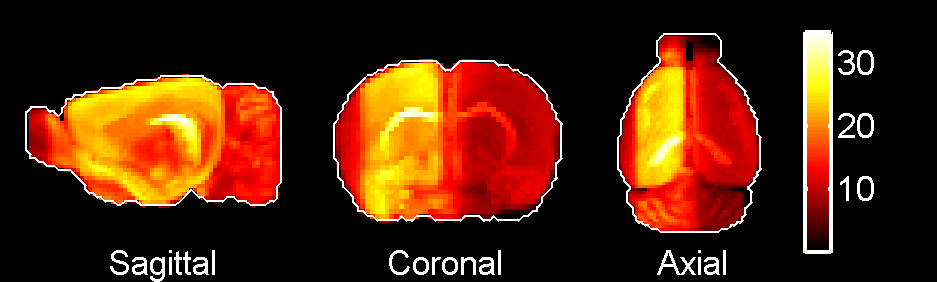
Figure 1: Maximal-intensity projections of the sum of all gene-expression profiles in the atlas (from both sagittal and coronal series). The left hemisphere has higher intensity then the right hemisphere due to the larger number of series covering it. However, the anatomical heterogeneity patterns (highlighting the hippocampus for instance), apart from intensity, seem to be left-right symmetric. However, there is a darker area on the left hemisphere that reveals missing sections from the sagittal series: indeed in this region the slices ae extremely small and fragile. The same issue is encountered in the most frontal sections of the olfactory buln in the coronal series.

2.2 Simulation of variability

For computational purposes we have the choice between $N(g)$ expression profiles for gene labeled $g$. Hence, instead of just one voxel-by-gene matrix whose $g$-th column contains $\left(E^{(1)}(v,g)\right)_{1\leq v\leq V}$, the ABA gives rise to a family of $\prod_{g=1}^{G}N(g)$ voxel-by-gene matrices, with voxels belonging to the left hemisphere. Any quantity computed from $E^{(1)}$ can be recomputed from any of these matrices, thereby inducing a distribution for this quantity, from which we can estimate quantities such as mean, median, variance and density. This is a finite but prohibitively large number of computations (at least $2^{G}$, given that each gene in the coronal atlas has at least two image series) to be performed, so for practical purposes we have to take a Monte Carlo approach and to perform the computation for $R$ random choices of data. The simulation of the distribution of a quantity $Q$ depending on the atlas can be obtained by the following pseudo-code:
for all $i$ in $[1..R]$
1. for all $g$ in [1..G], choose an integer $n_{i}(g)$ in $[1..N(g)]$
2. construct the matrix $E_{[i]}$ with entries $E_{[i]}(v,g)=E^{(n_{i}(g))}(v,g)$
3. compute the quantity $Q$ using this matrix, call the result $Q_{[i]}$
end
The larger $R$ is, the more precise the estimates for the distribution of the quantity $Q$ will be.

2.3 Correlation between the ABA and cell-type-specific microarray data

As an application, consider the correlation profile between the ABA and cell-type-specific transcriptome profiles collated in [25]. The microarray reads are arranged into a matrix $C$, whose rows correspond to cell types and whose columns correspond to genes (arranged in the same orders as in the matrix presentation of the ABA expression energies): $C(t,g)$ is the microarray read for gene labeled $g$ in the cell-type-specific sample labeled $t$, in the notations of [20], were the index $t$ take values between $1$ and $T=64$, and $g$ takes values getween $1$ and $G=2,131$, which is the number of genes found in [20] to be found both in the coronal ABA and in all the microarray reads). If we represent the ABA by a matrix $E_{[i]}$ of ISH data in the left hemisphere, obtained by drawing a random set in step 2 of the pseudo-code, the value of the brain-wide correlation at voxel $v$ with cell type $t$ reads:

$$\mathrm{Corr}_{[i]}(v,t)=\frac{\sum_{g=1}^{G}\left(C(t,g)-\frac{1}{T}\sum_{t=1}^{T}C(t,g)\right)\left(E_{[i]}(v,g)-\frac{1}{V}\sum_{v=1}^{V}E_{[i]}(v,g)\right)}{\sqrt{\sum_{k=1}^{G}\left(C(t,k)-\frac{1}{T}\sum_{t=1}^{T}C(t,k)\right)^{2}\sum_{h=1}^{G}\left(E_{[i]}(v,h)-\frac{1}{V}\sum_{v=1}^{V}E_{[i]}(v,h)\right)^{2}}},$$ (1)

and $v$ takes values corresponding to the left hemisphere. Having computed the family of correlation matrices $(\mathrm{Corr}_{[i]})_{1\leq i\leq R}$, we can study the distribution of their $t$-th column for each $t$. For example we can compute the average correlation profile (where the average is performed over the index $i$ labling the choice of image series):

$$\langle\mathrm{Corr}(v,t)\rangle=\frac{1}{R}\sum_{i=1}^{R}\mathrm{Corr}_{[i]}(v,t).$$ (2)

Moreover, we can estimate the dispersion of the correlation values for a cell type labeled $t$ and a region labeled $V_{r}$ in the ARA. For each random family of data (labeled by index $i$), we can compute the average correlation in the voxels belonging to region $V_{r}$ according to the ARA (this time the average is performed over voxels and the index of image series is not summed over):

$$\mathrm{Corr}_{r,[i]}(t)=\frac{1}{|V_{r}|}\sum_{v\in V_{r}}\mathrm{Corr}_{[i]}(v,t).$$ (3)

For a fixed value of $t$, this computation furnishes us with one family of $R$ numbers in the interval $[-1,1]$ for each region in the ARA. For the correlation analyis of [20] to be stable under a change of animal and sectioning modality, these families of numbers should come from a probability density that presents a peak.

2.4 Density estimates of cell types

The linear model proposed in [20] estimates the density profiles of cell types characterized by the transcriptome profile, assuming the expression energy of each gene is proportional to the number of mRNA molecules at each voxel, and that the microarray read of each gene in a cell type is also proportional to the number of mRNAs for this gene in this cell type. The expression energy at voxel labeled $v$ must be a a sum of cell-type-specific microarray reads, weighted by the density of each type at each voxel:

$$E(v,g)=\sum_{t}\rho_{t}(v)C(t,g),$$ (4)

where index $t$ labels cell types. In [20], we estimated the density profiles $(\rho_{t}(v))$ for all voxels $v$ in the mouse brain and for the cell types belonging to the data set collated in [25]. This estimation process was based on minimizing the difference between the l.h.s. and r.h.s. of Eq. 4 over all the possible positive coefficients $\rho$. This optimization procedure is deterministic, and relating the result to the mean density (decomposing the density into the sum of its mean and Gaussian noise) is a difficult problem in statistics (see [29]).

Some error estimates on the value of $\rho_{t}(v)$ were obained in [20, 22] using sub-sampling techniques, which involved mutilating the data by keeping only a random 10% of the coronal ABA, refitting the model, and repeating the operation. This induces a ranking of the cell types based on the stability of the results against sub-sampling. However, the set of genes on which the computation is based changes for each computation, and the fraction 10% is arbitrary (even though it is close to the fraction of the genome represented by our coronal data set). Having integrated the sagittal data into the atlas, we can now refit the model with the same sets of genes, only changing the set of image series from which they come, and we can do so in $\prod_{g=1}^{G}N(g)$ different ways. The only price we have to pay for this is the restriction of the results to the left hemisphere. This operation is just another application of the procedure outlined in the pseudo-code, with the role of the quantity $Q$ played by the family of numbers $\left(\rho_{t}(v)\right)_{1\leq t\leq T,}$, for all voxels $v$ in the left hemisphere.
With the notations introduced above, we denote by $(\rho_{t,{[i]}}(v))$ the density estimate obtained from the random matrix of ISH data $E_{[i]}$:

$$E_{[i]}(v,g)=\sum_{t}\rho_{t,[i]}(v)C(t,g)+{\mathrm{Residual}}(v,g).$$ (5)

We can group the voxels by region according to the ARA as we did for correlations in order to compare the results to classical neuroanatomy. The average density across random draws of image series for cell type lebeled $t$ reads:

$$\langle\rho_{t}(v)\rangle=\frac{1}{R}\sum_{i=1}^{R}\rho_{t,[i]}(v).$$ (6)

Since the number of cells of a given type in an extensive quantity, we compute the fraction of the total density contributed by each region, rather than the average density $\phi{r,[i]}(t)$ in region labeled $r$ for sample labeled $i$ and cell-type labeled $t$ :

$$\phi_{r,[i]}(t)=\frac{1}{\sum_{v\in\mathrm{left\;hemisphere}}\rho_{[i],t}(v)}\sum_{v\in V_{r}}\rho_{t,[i]}(v).$$ (7)

3 Results

3.1 Distributions of correlations give rise to peaks

After running simulations, we computed the average correlati8on profiles defined in Eq. 2. This quantity is plotted is plotted as a heat map on Fig. 2 for medium spiny neurons ($t=16$) and granule cells ($t=20$), from which it is clear that the average correlation profile presents a plateau inside the striatum for medium spiny neurons and inside the cerebellum for granule cells (which was also the case in [20] were the correlation profiles between the coronal atlas and cell types were analyzed).
Choosing brain regions from the coarsest version of the ARA, we computed the regional averages of correlation profiles defined in Eq. 3. The resulting families of numbers in the interval $[-1,1]$ were subjected to density estimation (based on kernel methods in MATLAB). The estimated densities present peaks. Moreover, the peaks are localized at higher values of correlation for the regions that present striking correlation patterns. Results of density estimation for medium spiny neurons ($t=16$) and granule cells ($t=20$) are presented on Fig. 3. In both cases the densities are peak-shaped, and the peak corresponding to the highest average correlation corresponds to the expected region, and is well decoupled from the other peaks: the peak corresponding to the striatum for the medium spiny neurons is centered at $0.29$, and entirely supported in the interval $[0.27,0.31]$, in which none of the quantities $\mathrm{Corr}_{r,[i]}(16)$ is found for values of $r$ not corresponding to the striatum. These results induce reassuring bounds pointing at the stability of the results of [20, 21], even though the dark areas in the coronal and axial projections of Fig. 2a probably corresponds to an artifically low expression energy in the most lateral part of the left hemisphere, due to missing sections in sagittal series. This effect is probably bringing down the average correlation between the cortex and the medium spiny neurons, but it concerns only a small fraction of the cortex, and the correlation in the most lateral sections estimated from coronal series only is close to the cortical average.

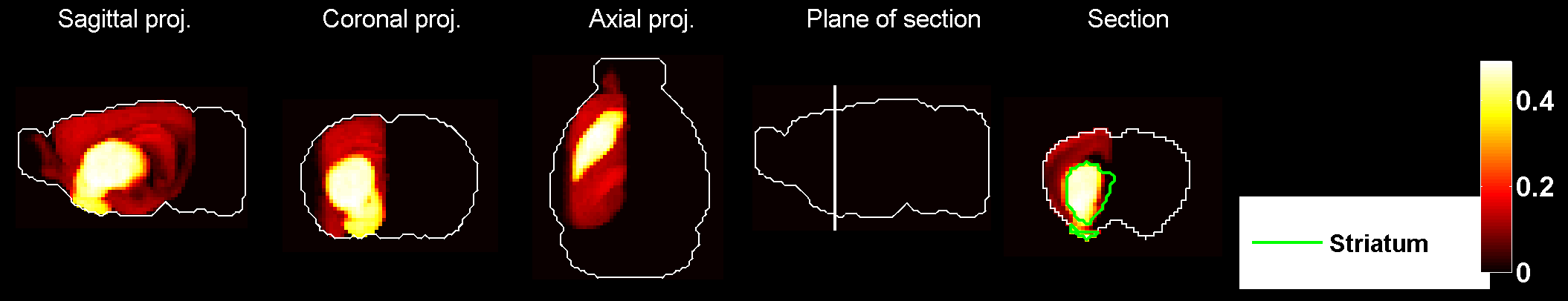
(a)

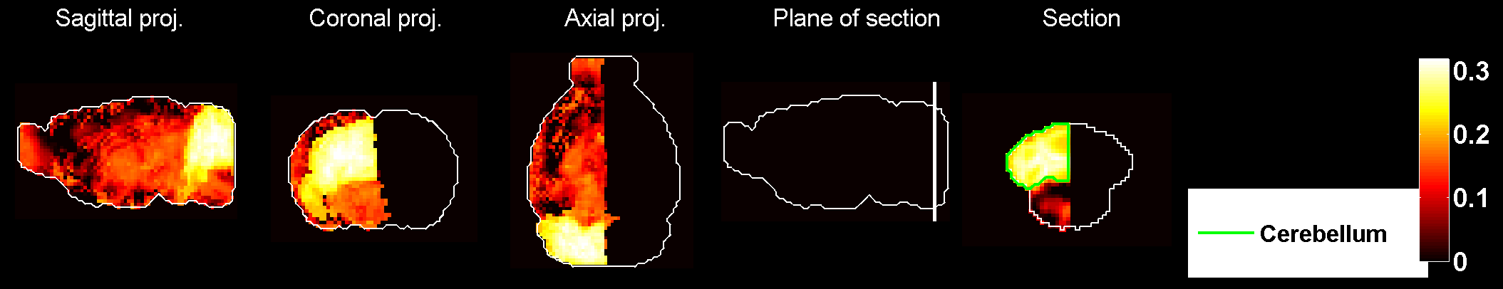
(b)

Figure 2: Heat maps of the average correlation between random image series from the ABA and cell-type-specific microarray data, $\langle\mathrm{Corr}(v,t)\rangle$, defined in Eq. 2. (a) For medium spiny neurons, $t=16$. (b) For granule cells, $t=20$. The sections were taken through the region in the ARA in which the correlation is highest on average (the boundary of this region defined by the ARA is outlined in green on the section).

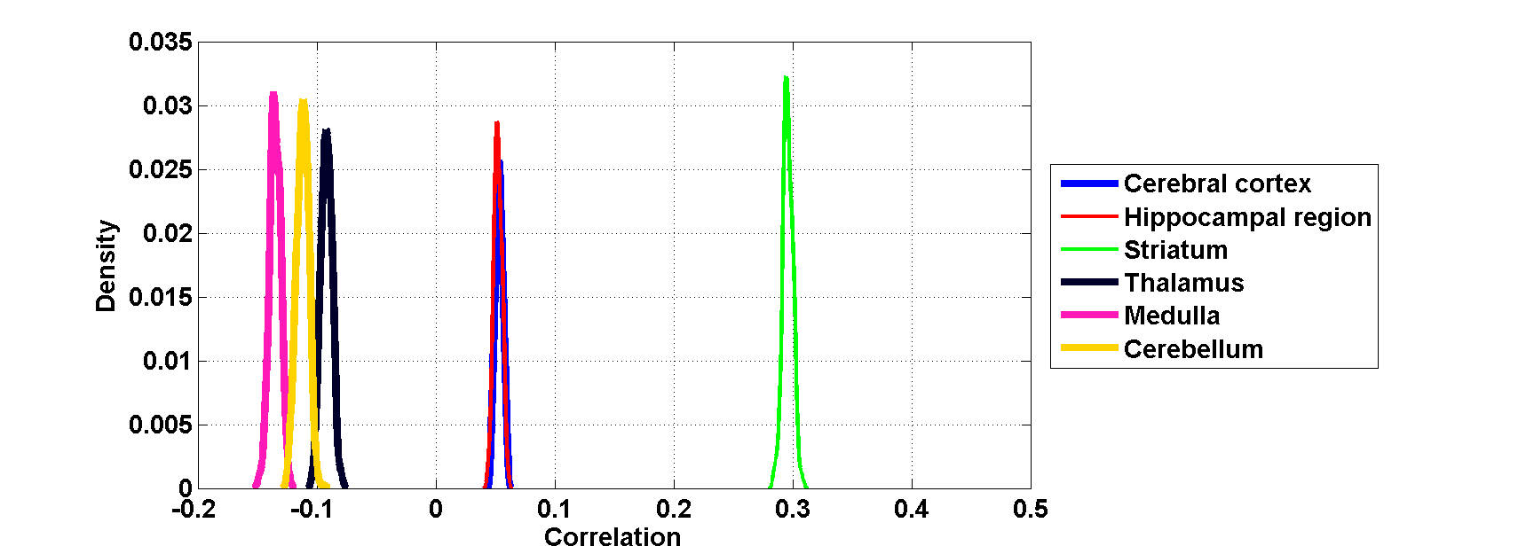
(a)

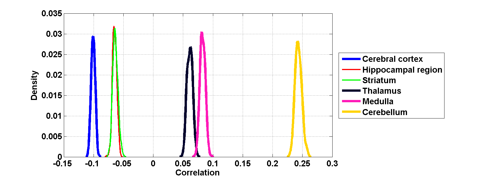
(b)

Figure 3: Estimated probability densities of the correlation profiles agglomerated in a few regions of the coarsest versions of the ARA. All the region-specific densities give rise to peaks. The right-most peak is well-decoupled from the others in both cases. (a) For medium spiny neurons, $t=16$; the peak centered at the highest value corresponds to the striatum. (b) For granule cells, $t=20$; the peak centered at the highest value corresponds to the cerebellum.

3.2 Peaks for the density of cell types are better separated than for correlations

Having refitted the linear model (Eq. 4) for each random draw of image series, we can plot the induced average density profiles for the same two cell types as above (see Fig. 4), which by eye gives a strong impression of the caudoputamen and of the granular layer of the cerebellum in the left hemisphere. Moreover, we estimated the densities of the contribution of each region in the coarsest version of the ARA to the total density of each cell type (Eq. 7). The resulting densities are supported in the interval $[0,1]$ by construction, and due to the fact the contributions from each region to the total density sum to 1 in each sample, the righjt-most peaks have a tendency to be more clearly decoupled from the others than in the correlation analysis. In particular, we can read from Fig. 5a that medium spiny neurons have $93(\pm 3)$ percent supported in the striatum, and from Fig. 5b similar numbers for granule cells in the cerebellum, without any region gathering more than 5 percent of the signal in any of the randoim samples.

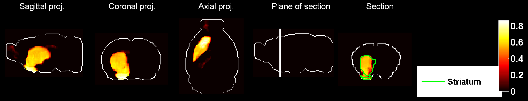
(a)

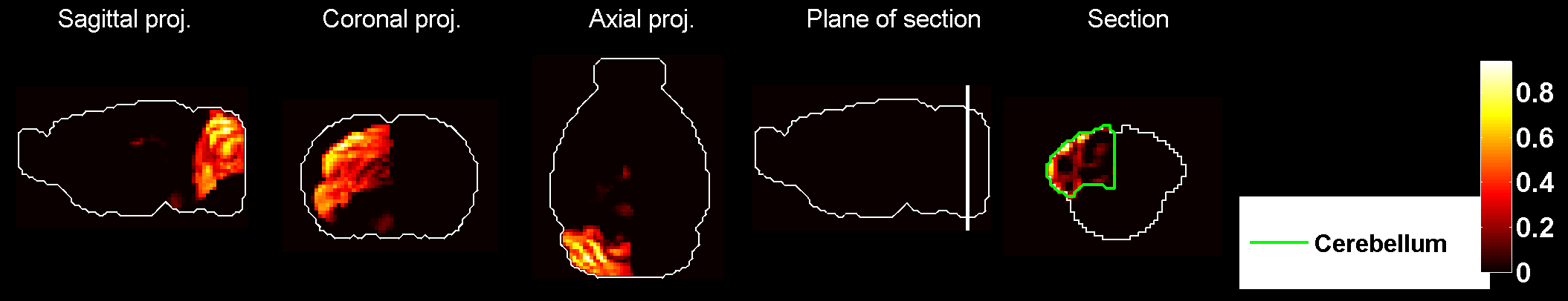
(b)

Figure 4: Heat maps of the average density of cell types in the left hemisphere, $\langle\mathrm{Corr}(v,t)\rangle$, defined in Eq. 6. (a) For medium spiny neurons, $t=16$. (b) For granule cells, $t=20$. They are visually very close to the heat maps of $\rho_{16}$ and $\rho_{20}$ obtained in [20].

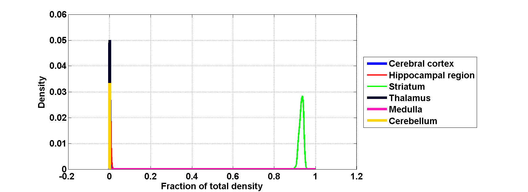
(a)

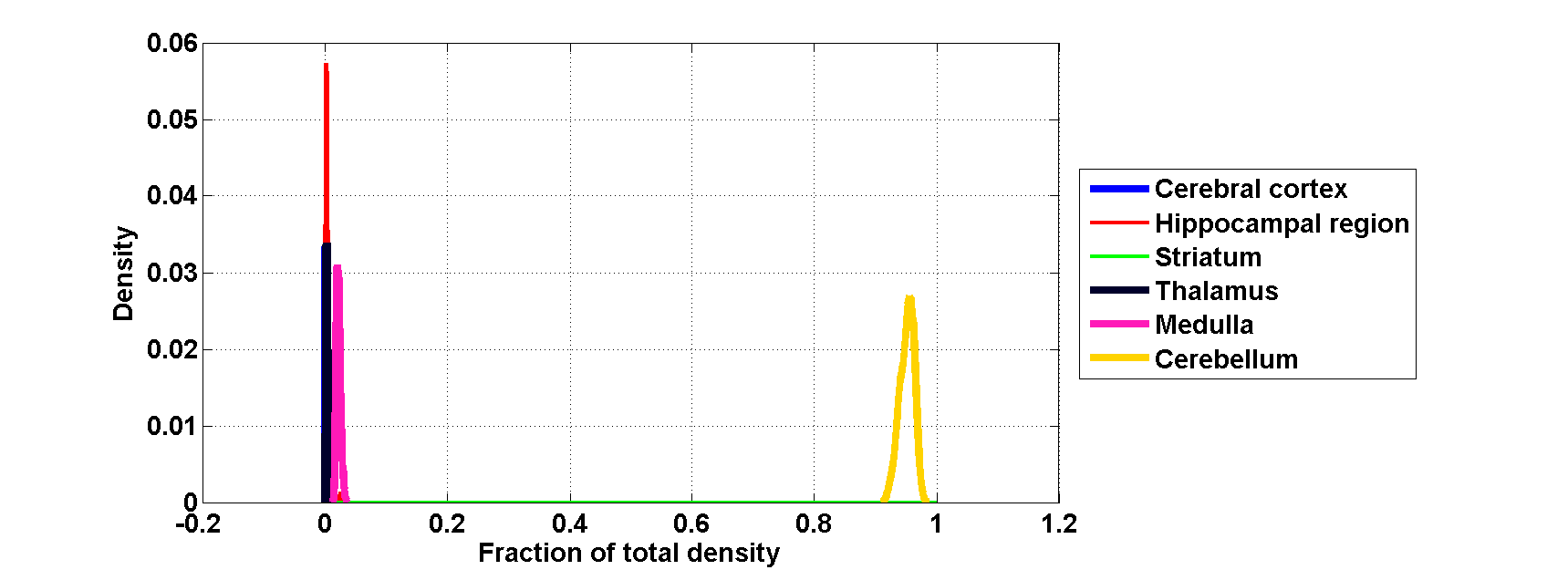
(b)

Figure 5: Estimated probability densities of fractions of density agglomerated in a few regions of the coarsest versions of the ARA (see Eq. 7). All the region-specific densities give rise to peaks. The right-most peak is well-decoupled from the others in both cases, furthermore the other peaks are all centered close to zero (making several of them almost invisible). (a) For medium spiny neurons, $t=16$; the peak centered at the highest value corresponds to the striatum. (b) For granule cells, $t=20$; the peak centered at the highest value corresponds to the cerebellum.

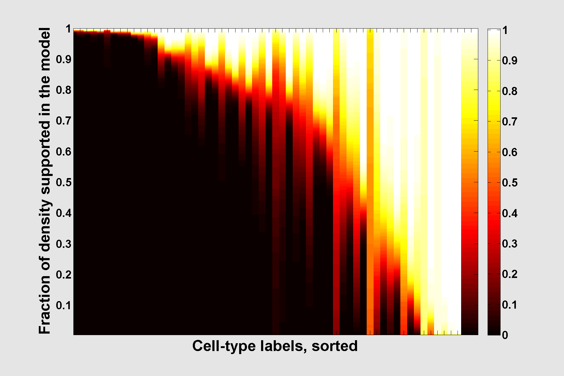
Figure 6: A heat map of the CDFs of the random overlaps with the results of the model based on the coronal atlas.

The two cases exposed in Figs. 3 andfittingDistrs serve as proof of concept, because medium spiny neurons and granule cells are well-studied cell types, independently from the neurome approach of [11], and they are expected to be strongly associated to the striatum and cerebellum respectively. However, some cell types may exhibit more complex neuroanatomical patterns of density, and breaking the estimated density according to the coarsest version of the ARA as in Eq. 7. To study neuroanatomy in a purely data-driven way, we must not use any input from classical neuroanatomy. For a given cell type, we must compare the family of density profiles $(\rho_{[i],t})_{1\leq i\leq R}$ to the density profile $\rho_{t}$ estimated from the coronal atlas. A possible comparison, proposed in [20] to analyze the results of the sub-sampling simulations, involves the computation of the overlap between density profiles:

$${\mathcal{I}}(i,t):=\frac{1}{\sum_{v}\rho_{[i],t}(v)}\sum_{v}{\mathbf{1}}(\rho_{t}(v)>0)\rho_{[i],t}(v),$$ (8)

which is the fraction of the total estimated density in the $i$-th draw supported by the coronal model. For each cell-type label $t$, the overlap ${\mathcal{I}}(.,t)$ is a random variable, whose distribution can be studied using the empirical cumulative distribution function (CDF) as follows:

$${\mathrm{\sc{CDF}}}(u,t)=\frac{1}{S}\left|\left\{i\in[1..R],{\mathcal{I}}(r,t)\leq u\right\}\right|.$$ (9)

If we present the CDFs in matrix form, with one cell type per column, and rows corresponding to the value of the overlap, we can plot this matrix as a heat map, as on Fig. 6. The more stable the model is for a cell type, the larger the dark area in the corresponding column is. This Figure has a much larger dark area than the analogous Figure in [20], in which the random step involved taking a random 10% of the genes and refitting the model. For instance, 10 cell types have an overlap of more than 95 % with the original model with probability 1, which was not the case for any of the cell types according to the sub-sampling procedure. The computational treatment of the full set of image series therefore reveals stronger stability properties of the linear model.

3.3 Ranking of cell types by stability of results

Let us recall the notations introduced in [22] to analyze the results of the simulated distribution of overlaps with the orioginal (coronal) model.

Having simulated the distribution of the sub-sampled densities of all the $T$ cell-type specific transcriptomes in our data set, we can estimate confidence thresholds in two ways, for a cell type labeled $t$.

(1) Impose a threshold $\alpha$ in the interval $[0,1]$ on the overlap with the density $\rho_{t}$ estimated in the linear model, and work out the probability $p_{t,\alpha}$ of reaching that threshold from the sub-samples:

$$p_{t,\alpha}:=P(\mathcal{I}(.,t)\geq\alpha)=\frac{1}{S}\left|s\in[1..S],\mathcal{I}(s,t)\geq\alpha\right|.$$ (10)

For a cell type labeled $t$, the distribution of the overlaps ${\mathcal{I}}(.,t)$ can be visualized using the cumulative distribution function ${\mathrm{\sc{CDF}}}_{t}$ (in the space $[0,1]$ of the values of the overlap between $\rho_{t}$ sub-sampled profiles $\rho_{t}^{(s)}$):

$${\mathrm{\sc{CDF}}}_{t}(\alpha)=\frac{1}{S}\left|\left\{s\in[1..S],{\mathcal{I}}(s,t)\leq\alpha\right\}\right|.$$ (11)

The value ${\mathrm{\sc{CDF}}}_{t}(u)$ is related to the probability defined in Eq. 10 as follows:

$$p_{t,\alpha}=1-{\mathrm{\sc{CDF}}}_{t}(\alpha).\\$$ (12)

(2) Impose a threshold $\beta$ in the interval $[0,1]$ on the fraction of sub-samples, and work out which overlap $\mathcal{I}_{thresh}(t,\beta)$ with the estimated density $\rho_{t}$ is reached by that fraction of the sub-samples. The threshold value of the intercept $\mathcal{I}_{thresh}(t,\beta)$ is readily expressed in terms of the inverse of the cumulative distribution function:

$$\mathcal{I}_{thresh}(t,\beta)={\mathrm{\sc{CDF}}}_{t}^{-1}(\beta).$$ (13)

The more stable the prediction $\rho_{t}$ is again sub-sampling, the more concentrated the values of ${\mathcal{I}}(.,t)$ are at high values (close to 1), the slower the take-off of the cumulative function ${\mathrm{\sc{CDF}}}_{t}$ is, the lower the value of ${\mathrm{\sc{CDF}}}_{t}(\alpha)$ is, and the larger the probablity $p_{t,\alpha}$ is (for a fixed value of $\alpha$ in [0,1]).

For a fixed cell type labeled $t$, the values of $p(t,.)$ and $\mathcal{I}_{thresh}(t,.)$ can therefore be readily read off from a plot of the cumulative distribution function $\mathrm{\sc{CDF}}$ (this plot is in the $\alpha\beta$ plane in our notations). For the sake of visualization of results for all cell types, we constructed the matrix ${\mathcal{P}}$, whose columns correspond to cell types, and whose rows correspond to values of the threshold $\alpha$:

$${\mathcal{P}}(\alpha,r_{t}^{signal}):={\mathrm{\sc{CDF}}}_{t}(\alpha),$$ (14)

where the index $r_{t}^{signal}$ in the l.h.s. means that the cell types are ordered by decreasing order of overlap between the average sub-sampled profile and the predicted profile. If the entries of the matrix $\mathcal{P}$ are plotted as a heat map (see Fig. 6), the hot colors will be more concentrated in the left-most part of the image. For a fixed column, the more concentrated the hot colors are in the heat map, the more stable the corresponding cell type is.

4 Discussion

The present work allows to bring the power of the online facilities of the ABA to the desktop for a collective analysis of gene-expression energies. The example of the analysis of correlation with microarray data sets shows the power of the ABA as a tool of analysis for other data sets. This goes beyond the correlation structure of the ABA itself, and its relation to the classical neuroanatomy of the ARA, that can elready be investigated online using the Anatomic Gene Expression Atlas (AGEA, see [2]).

When the coronal ABA was used to analyze other data sets, in particular microarray data as in [20], it was assumed that it reflects an average collective expression of the genome in the adult mouse brain, showing little sensitivity to dynamics and to animal-to-animal variations, even though each expression profile comes from a different animal. The fact that correlation profiles allowed to guess the anatomical origin of many cell types in [20] provided a self-consistent check of this assumption, but incorporating the different ISH image series into the computational analysis allows to control the numerical errors in the correlation profiles.

Moreover, the Monte Carlo approach we took to simulate the variability of region-specificity is much more consistent than the sub-sempling approach taken in [20]. The numerical results show a greater stability than in the sub-sampling approach on average.

It should be emphasized that the computations in the present paper only serve as examples, bringing more accurate answers to the most current questions posed by the analysis of the ABA. Ultimately, the distribution of any quantity based on the atlas can be computed exactly and studied at each voxel, without the need to agglomerate voxels into neuroanatomical regions.

5 Tables: cell-type-specific transcriptomes: description, labeling and anatomical origin

For each of the cell-type-specific samples analyzed in this note, the following two tables give a brief description of the cell type, the region from which the samples were extracted according to the coarsest version of the Allen Reference Atlas, and the finest region to which it can be assigned according to the data provided in the studies [18, 14, 16, 17, 12, 13, 15, 11]. The indices in the first columns of the tables are the ones refered to as $t$.

Index	Description	Region in the ARA (’big12’)	Finest label in the ARA
1	Purkinje Cells	Cerebellum	Cerebellar cortex
2	Pyramidal Neurons	Cerebral cortex	Primary motor area; Layer 5
3	Pyramidal Neurons	Cerebral cortex	Primary somatosensory area; Layer 5
4	A9 Dopaminergic Neurons	Midbrain	Substantia nigra_ compact part
5	A10 Dopaminergic Neurons	Midbrain	Ventral tegmental area
6	Pyramidal Neurons	Cerebral cortex	Cerebral cortex; Layer 5
7	Pyramidal Neurons	Cerebral cortex	Cerebral cortex; Layer 5
8	Pyramidal Neurons	Cerebral cortex	Cerebral cortex; Layer 6
9	Mixed Neurons	Cerebral cortex	Cerebral cortex
10	Motor Neurons, Midbrain Cholinergic Neurons	Midbrain	Peduncolopontine nucleus
11	Cholinergic Projection Neurons	Pallidum	Pallidum_ ventral region
12	Motor Neurons, Cholinergic Interneurons	Medulla	Spinal cord
13	Cholinergic Neurons	Striatum	Striatum
14	Interneurons	Cerebral cortex	Cerebral cortex
15	Drd1+ Medium Spiny Neurons	Striatum	Striatum
16	Drd2+ Medium Spiny Neurons	Striatum	Striatum
17	Golgi Cells	Cerebellum	Cerebellar cortex
18	Unipolar Brush cells (some Bergman Glia)	Cerebellum	Cerebellar cortex
19	Stellate Basket Cells	Cerebellum	Cerebellar cortex
20	Granule Cells	Cerebellum	Cerebellar cortex
21	Mature Oligodendrocytes	Cerebellum	Cerebellar cortex
22	Mature Oligodendrocytes	Cerebral cortex	Cerebral cortex
23	Mixed Oligodendrocytes	Cerebellum	Cerebellar cortex
24	Mixed Oligodendrocytes	Cerebral cortex	Cerebral cortex
25	Purkinje Cells	Cerebellum	Cerebellar cortex
26	Neurons	Cerebral cortex	Cerebral cortex
27	Bergman Glia	Cerebellum	Cerebellar cortex
28	Astroglia	Cerebellum	Cerebellar cortex
29	Astroglia	Cerebral cortex	Cerebral cortex
30	Astrocytes	Cerebral cortex	Cerebral cortex
31	Astrocytes	Cerebral cortex	Cerebral cortex
32	Astrocytes	Cerebral cortex	Cerebral cortex
33	Mixed Neurons	Cerebral cortex	Cerebral cortex
34	Mixed Neurons	Cerebral cortex	Cerebral cortex
35	Mature Oligodendrocytes	Cerebral cortex	Cerebral cortex
36	Oligodendrocytes	Cerebral cortex	Cerebral cortex
37	Oligodendrocyte Precursors	Cerebral cortex	Cerebral cortex

Table 1: Anatomical origin of the cell-type-specific samples (I).

Index	Description	Region in the ARA (’big12’)	Finest label in the ARA
38	Pyramidal Neurons, Callosally projecting, P3	Cerebral cortex	Cerebral cortex
39	Pyramidal Neurons, Callosally projecting, P6	Cerebral cortex	Cerebral cortex
40	Pyramidal Neurons, Callosally projecting, P14	Cerebral cortex	Cerebral cortex
41	Pyramidal Neurons, Corticospinal, P3	Cerebral cortex	Cerebral cortex
42	Pyramidal Neurons, Corticospinal, P6	Cerebral cortex	Cerebral cortex
43	Pyramidal Neurons, Corticospinal, P14	Cerebral cortex	Cerebral cortex
44	Pyramidal Neurons, Corticotectal, P14	Cerebral cortex	Cerebral cortex
45	Pyramidal Neurons	Cerebral cortex	Cerebral cortex, Layer 5
46	Pyramidal Neurons	Cerebral cortex	Cerebral cortex, Layer 5
47	Pyramidal Neurons	Cerebral cortex	Primary somatosensory area; Layer 5
48	Pyramidal Neurons	Cerebral cortex	Prelimbic area and Infralimbic area; Layer 5 (Amygdala)
49	Pyramidal Neurons	Hippocampal region	Ammon’s Horn; Layer 6B
50	Pyramidal Neurons	Cerebral cortex	Primary motor area
51	Tyrosine Hydroxylase Expressing	Pons	Pontine central gray
52	Purkinje Cells	Cerebellum	Cerebellar cortex
53	Glutamatergic Neuron (not well defined)	Cerebral cortex	Cerebral cortex; Layer 6B (Amygdala)
54	GABAergic Interneurons, VIP+	Cerebral cortex	Prelimbic area and Infralimbic area
55	GABAergic Interneurons, VIP+	Cerebral cortex	Primary somatosensory area
56	GABAergic Interneurons, SST+	Cerebral cortex	Prelimbic area and Infralimbic area
57	GABAergic Interneurons, SST+	Hippocampal region	Ammon’s Horn
58	GABAergic Interneurons, PV+	Cerebral cortex	Prelimbic area and Infralimbic area
59	GABAergic Interneurons, PV+	Thalamus	Dorsal part of the lateral geniculate complex
60	GABAergic Interneurons, PV+, P7	Cerebral cortex	Primary somatosensory area
61	GABAergic Interneurons, PV+, P10	Cerebral cortex	Primary somatosensory area
62	GABAergic Interneurons, PV+, P13-P15	Cerebral cortex	Primary somatosensory area
63	GABAergic Interneurons, PV+, P25	Cerebral cortex	Primary somatosensory area
64	GABAergic Interneurons, PV+	Cerebral cortex	Primary motor area

Table 2: Anatomical origin of the cell-type-specific samples (II).

6 Tables of of rankings of cell types by estimates of overlap with the coronal model

$r^{signal}_{t}$	Cell type	Index $t$	$\bar{\mathcal{I}}(t)$, (%)	$p_{t,0.75}$, (%)	$\mathcal{I}_{thresh}(t,0.75)$, (%)
1	Granule Cells	20	99.5	100	99.2
2	Purkinje Cells	1	99.4	100	99.2
3	Motor Neurons, Cholinergic Interneurons	12	99.2	100	99.2
4	Pyramidal Neurons	47	99.1	100	99.2
5	Pyramidal Neurons	49	99.1	100	99.2
6	Glutamatergic Neuron (not well defined)	53	99.1	100	99.6
7	Mature Oligodendrocytes	35	99	100	98.8
8	Drd2+ Medium Spiny Neurons	16	98.9	100	98.8
9	Tyrosine Hydroxylase Expressing	51	98.9	100	98.8
10	Pyramidal Neurons, Callosally projecting, P14	40	98.3	100	98.4
11	Pyramidal Neurons	46	98	100	98.4
12	Astroglia	28	97.1	100	98.4
13	Pyramidal Neurons, Corticotectal, P14	44	96.9	100	97.7
14	Pyramidal Neurons	6	92.4	99.6	95.3
15	GABAergic Interneurons, PV+	64	92.2	100	93
16	GABAergic Interneurons, SST+	57	91.7	100	93.4
17	Astrocytes	31	91.1	99.4	93.4
18	Purkinje Cells	52	89.9	93.9	95.3
19	GABAergic Interneurons, SST+	56	88.2	95.7	93
20	GABAergic Interneurons, PV+	59	87	85.8	94.5
21	Mature Oligodendrocytes	21	87	100	88.3
22	Pyramidal Neurons	48	86.2	98.9	88.7
23	A10 Dopaminergic Neurons	5	85.7	84.1	93.4
24	Cholinergic Neurons	13	84.7	96.9	87.5
25	Pyramidal Neurons	45	82.8	97.7	85.2
26	GABAergic Interneurons, VIP+	55	81.6	75	89.5
27	Motor Neurons, Midbrain Cholinergic Neurons	10	80.7	94.1	82.8
28	A9 Dopaminergic Neurons	4	80.1	74.8	87.5
29	Oligodendrocyte Precursors	37	79.6	67.1	91.8
30	Mature Oligodendrocytes	22	79	78.4	81.6
31	Pyramidal Neurons, Callosally projecting, P3	38	78.5	70.9	95.7
32	Astrocytes	32	78.3	65.5	93

Table 3: Cell types ranked by average overlap with the coronal model (I).

$r^{signal}_{t}$	Cell type	Index $t$	$\bar{\mathcal{I}}(t)$, (%)	$p_{t,0.75}$, (%)	$\mathcal{I}_{thresh}(t,0.75)$, (%)
33	Stellate Basket Cells	19	77	64.5	80.1
34	GABAergic Interneurons, PV+, P7	60	76.3	57.1	89.5
35	Mixed Neurons	34	72.8	50.3	83.2
36	Pyramidal Neurons, Corticospinal, P14	43	69.9	48.2	87.1
37	Pyramidal Neurons	7	69	18.5	73.4
38	GABAergic Interneurons, VIP+	54	67.4	15	72.7
39	Astrocytes	30	63.5	9.9	69.1
40	Pyramidal Neurons, Callosally projecting, P6	39	56.2	40.5	89.1
41	Mixed Neurons	33	56.2	21.5	71.9
42	Oligodendrocytes	36	54.3	8.5	63.7
43	Pyramidal Neurons	50	44.4	9.7	62.9
44	Drd1+ Medium Spiny Neurons	15	42.8	-0.4	47.7
45	Golgi Cells	17	40.4	36.8	99.2
46	Pyramidal Neurons, Corticospinal, P6	42	32	9.3	48.8
47	GABAergic Interneurons, PV+, P25	63	30.4	-0.3	39.1
48	GABAergic Interneurons, PV+	58	26.2	0.6	35.5
49	Unipolar Brush cells (some Bergman Glia)	18	25	-0.4	31.3
50	GABAergic Interneurons, PV+, P10	61	17.9	3.1	29.3
51	Astroglia	29	14.1	-0.4	18
52	Pyramidal Neurons	8	12.1	0.1	14.1
53	Pyramidal Neurons	3	9.6	8	0.4
54	Neurons	26	4	0.1	5.9
55	Mixed Neurons	9	3.8	3.1	0.4
56	Bergman Glia	27	1.1	-0.4	0.4
57	Pyramidal Neurons	2	0.3	-0.4	0.4
58	GABAergic Interneurons, PV+, P13-P15	62	0	-0.4	0.4
59	Cholinergic Projection Neurons	11	0	22.2	71.9
60	Interneurons	14	0	22.2	71.9
61	Mixed Oligodendrocytes	23	0	22.2	71.9
62	Mixed Oligodendrocytes	24	0	22.2	71.9
63	Purkinje Cells	25	0	22.2	71.9
64	Pyramidal Neurons, Corticospinal, P3	41	0	22.2	71.9

Table 4: Cell types ranked by average overlap with the coronal model (II).

7 Cell-type-specific results

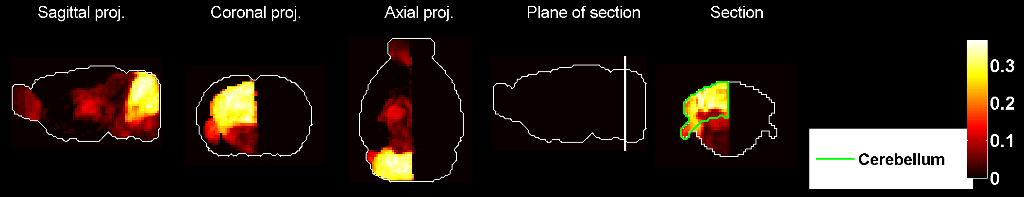
Figure 7: Heat map of the mean correlation profile for cell type labeled $1$.

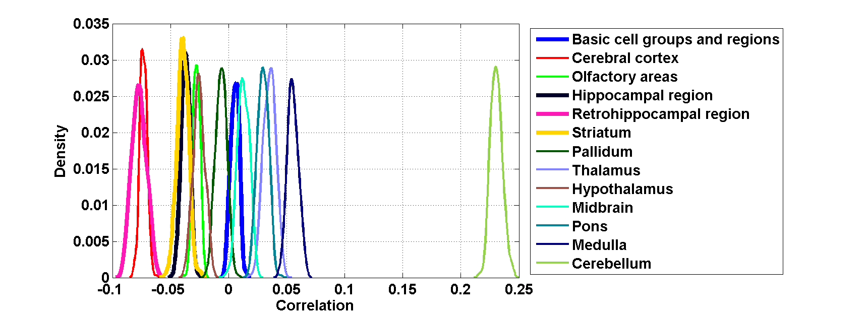
Figure 8: Distribution profiles of the correlations between transcriptome profile of cell type labeled $1$ across random sets of ISH expression energy profiles.

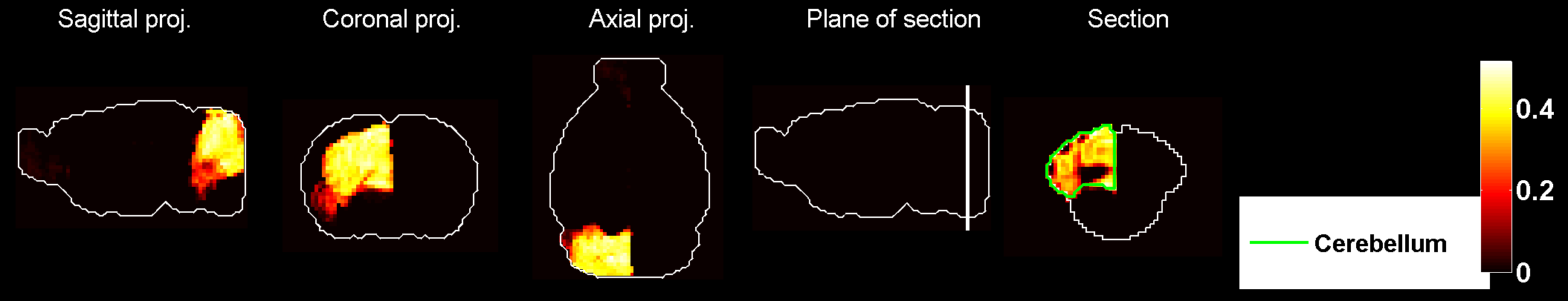
Figure 9: Heat map of the mean density profile for cell type labeled $1$.

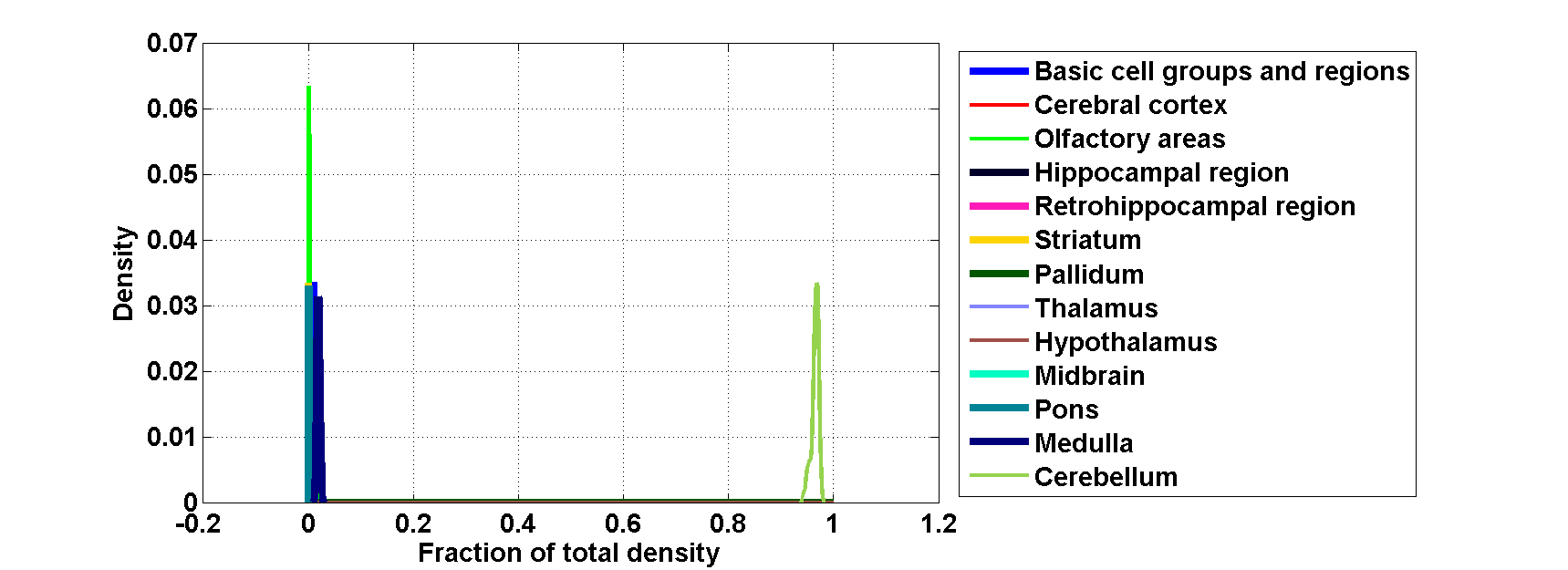
Figure 10: Distribution profiles of the density profile of cell type labeled $1$ across random sets of ISH expression energy profiles.

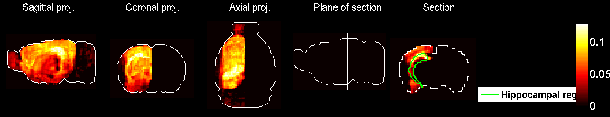
Figure 11: Heat map of the mean correlation profile for cell type labeled $2$.

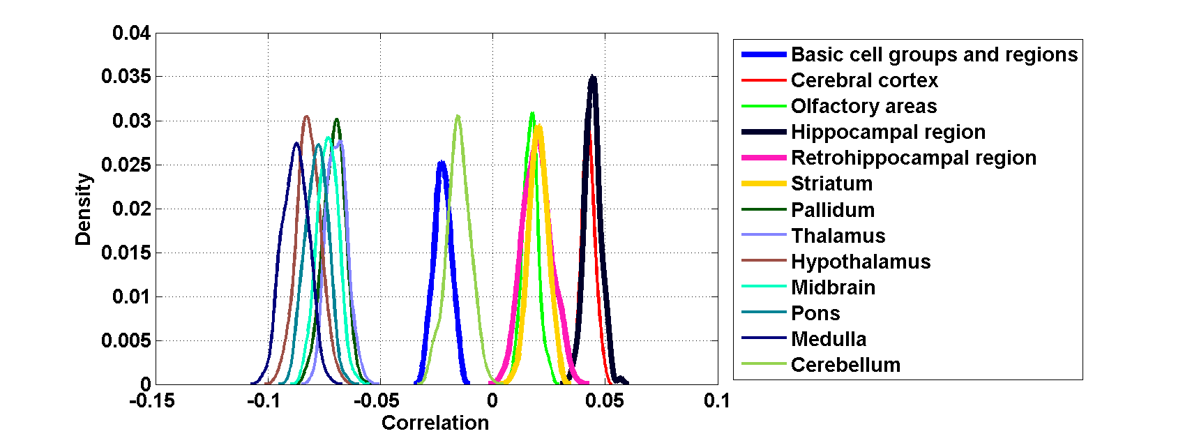
Figure 12: Distribution profiles of the correlations between transcriptome profile of cell type labeled $2$ across random sets of ISH expression energy profiles.

Figure 13: Heat map of the mean density profile for cell type labeled $2$.

Figure 14: Distribution profiles of the density profile of cell type labeled $2$ across random sets of ISH expression energy profiles.

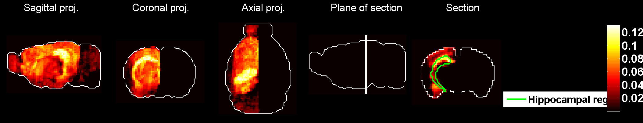
Figure 15: Heat map of the mean correlation profile for cell type labeled $3$.

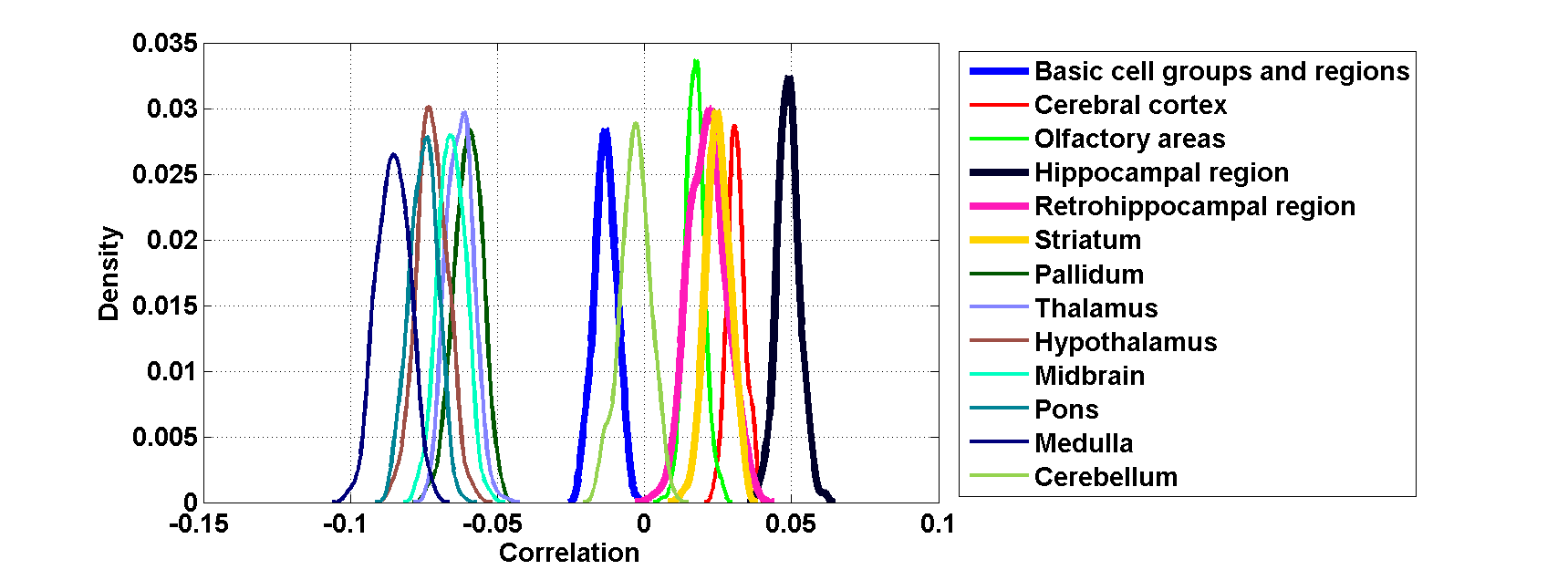
Figure 16: Distribution profiles of the correlations between transcriptome profile of cell type labeled $3$ across random sets of ISH expression energy profiles.

Figure 17: Heat map of the mean density profile for cell type labeled $3$.

Figure 18: Distribution profiles of the density profile of cell type labeled $3$ across random sets of ISH expression energy profiles.

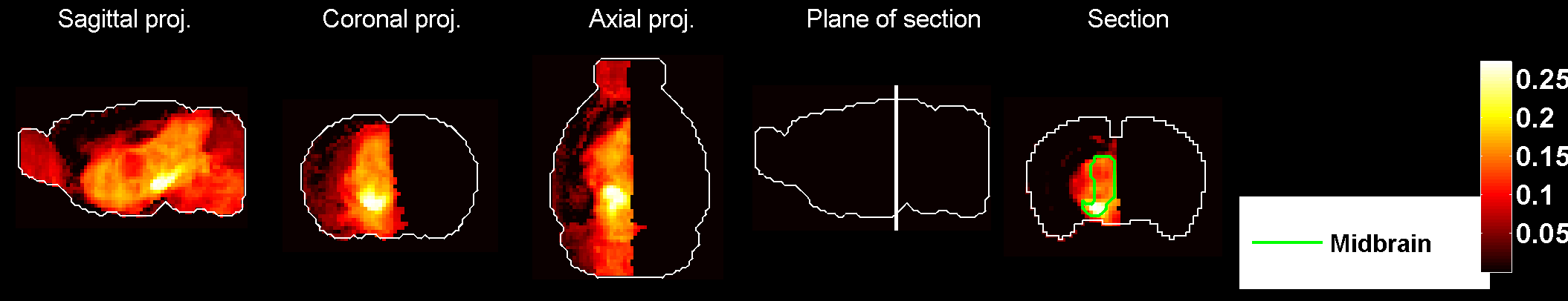
Figure 19: Heat map of the mean correlation profile for cell type labeled $4$.

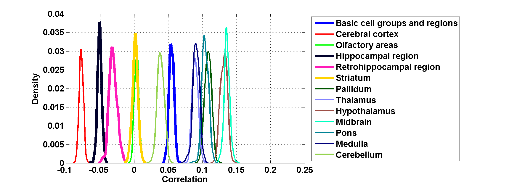
Figure 20: Distribution profiles of the correlations between transcriptome profile of cell type labeled $4$ across random sets of ISH expression energy profiles.

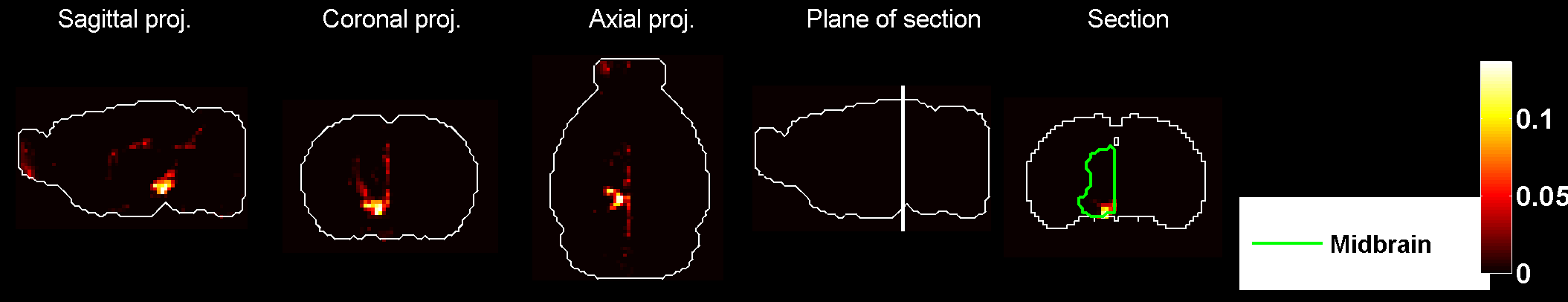
Figure 21: Heat map of the mean density profile for cell type labeled $4$.

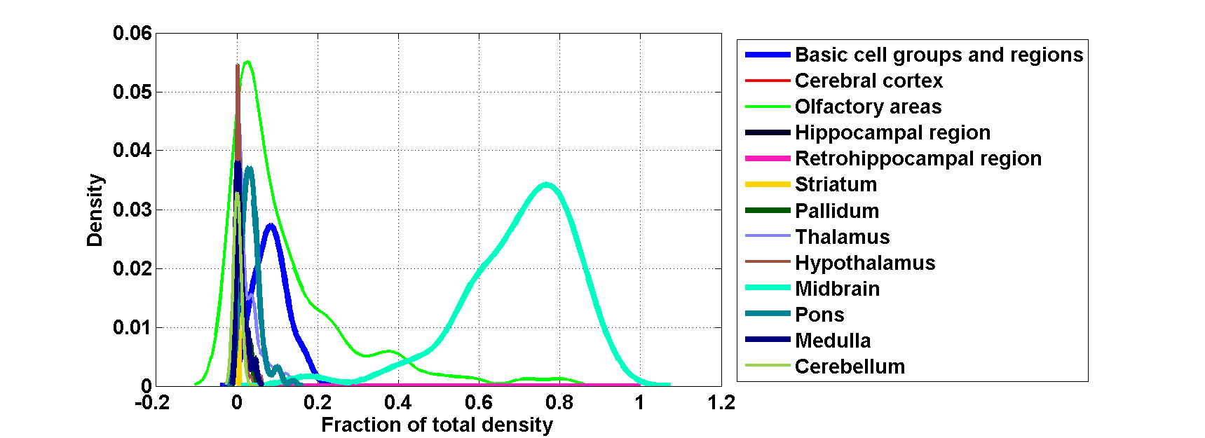
Figure 22: Distribution profiles of the density profile of cell type labeled $4$ across random sets of ISH expression energy profiles.

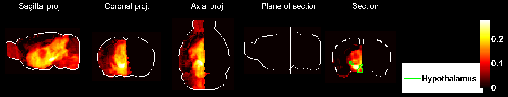
Figure 23: Heat map of the mean correlation profile for cell type labeled $5$.

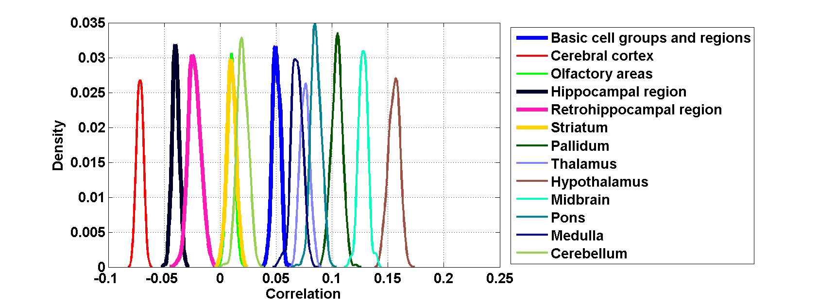
Figure 24: Distribution profiles of the correlations between transcriptome profile of cell type labeled $5$ across random sets of ISH expression energy profiles.

Figure 25: Heat map of the mean density profile for cell type labeled $5$.

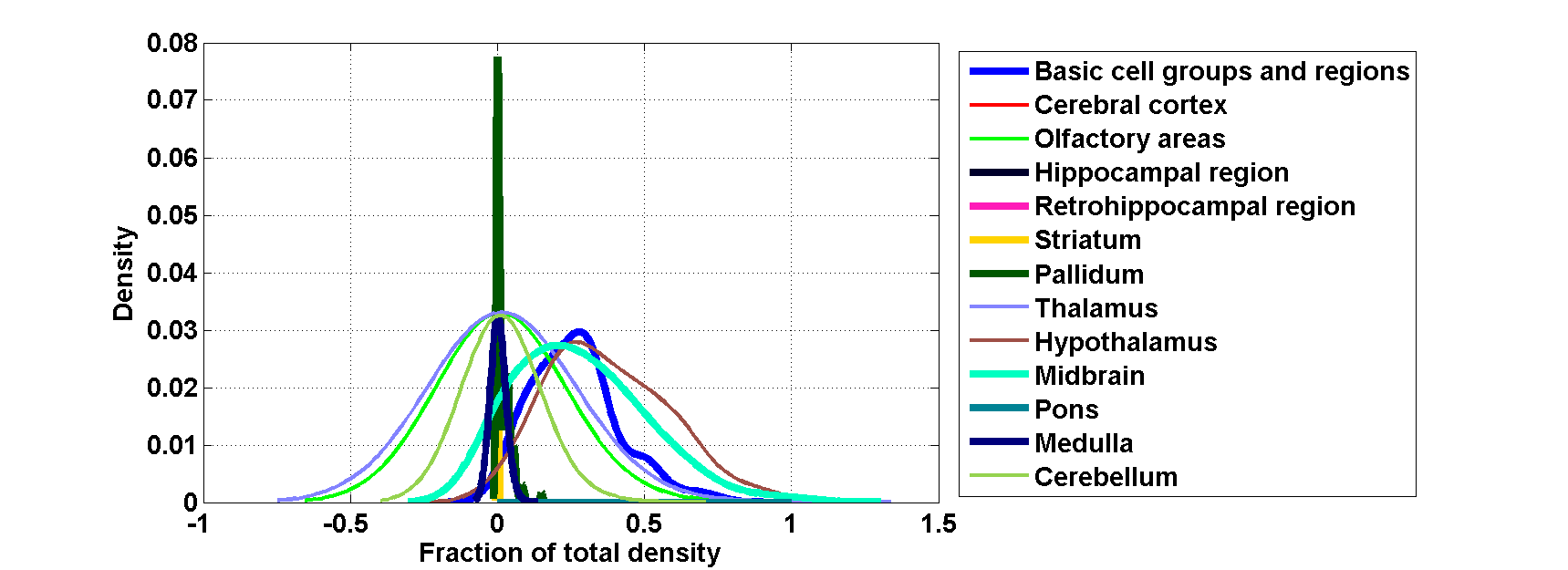
Figure 26: Distribution profiles of the density profile of cell type labeled $5$ across random sets of ISH expression energy profiles.

Figure 27: Heat map of the mean correlation profile for cell type labeled $6$.

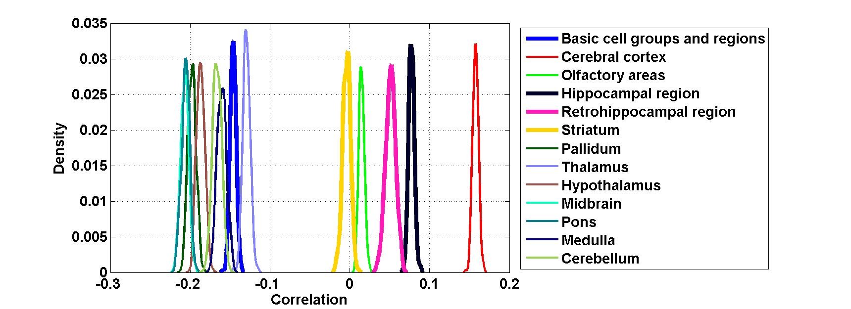
Figure 28: Distribution profiles of the correlations between transcriptome profile of cell type labeled $6$ across random sets of ISH expression energy profiles.

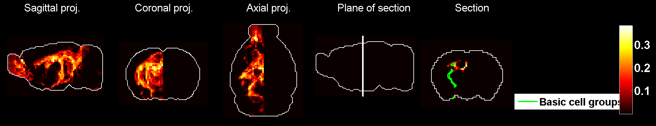
Figure 29: Heat map of the mean density profile for cell type labeled $6$.

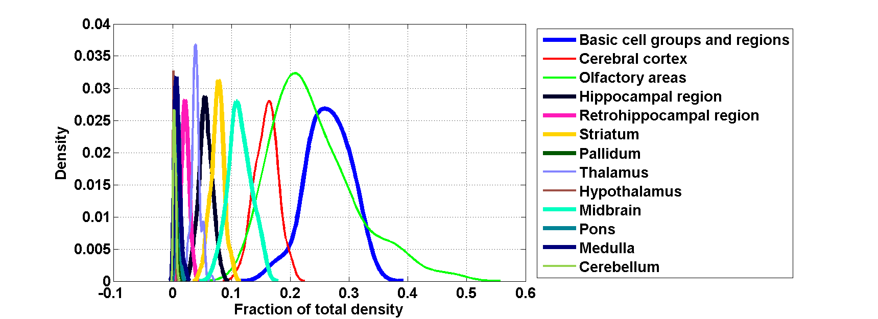
Figure 30: Distribution profiles of the density profile of cell type labeled $6$ across random sets of ISH expression energy profiles.

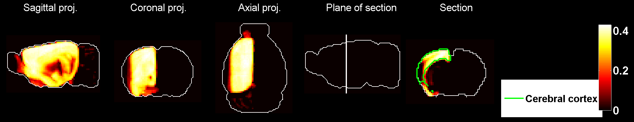
Figure 31: Heat map of the mean correlation profile for cell type labeled $7$.

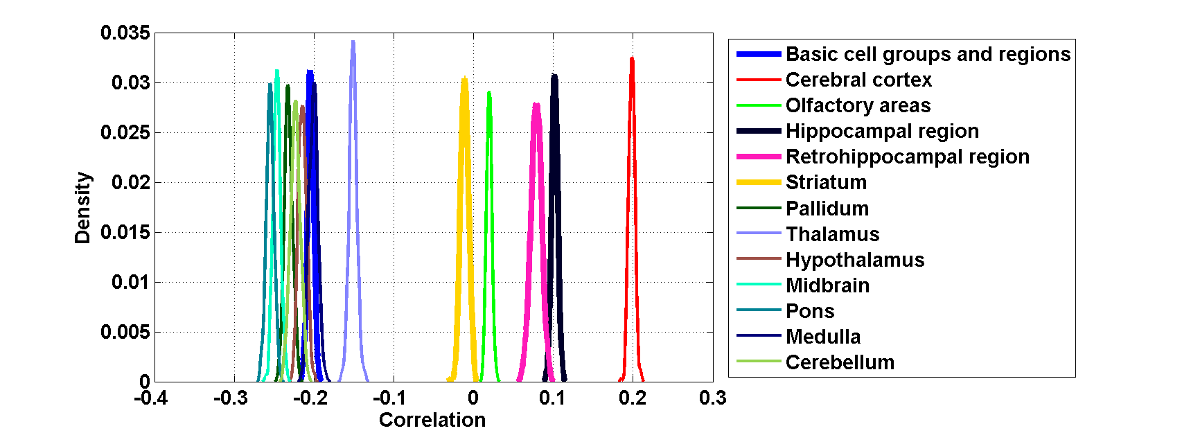
Figure 32: Distribution profiles of the correlations between transcriptome profile of cell type labeled $7$ across random sets of ISH expression energy profiles.

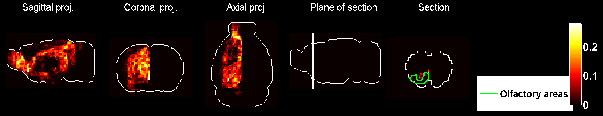
Figure 33: Heat map of the mean density profile for cell type labeled $7$.

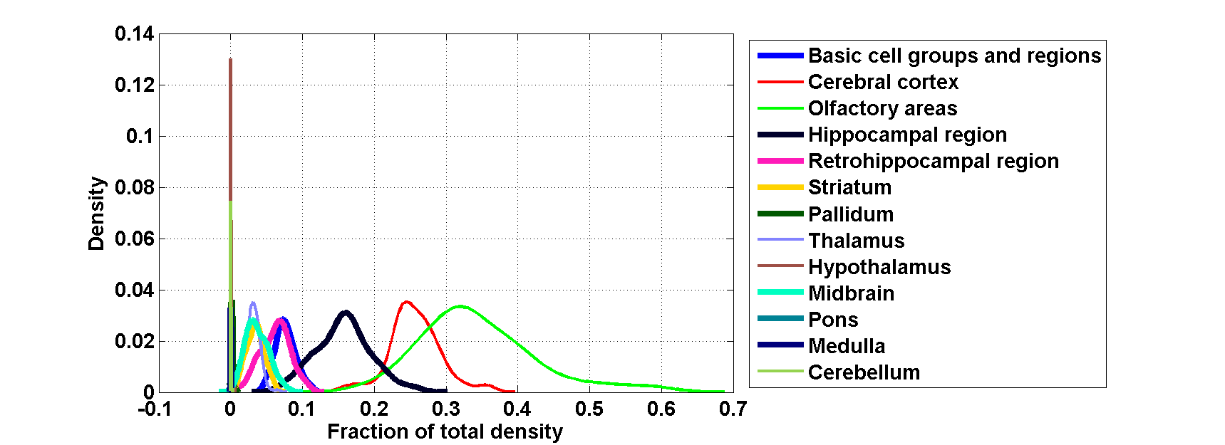
Figure 34: Distribution profiles of the density profile of cell type labeled $7$ across random sets of ISH expression energy profiles.

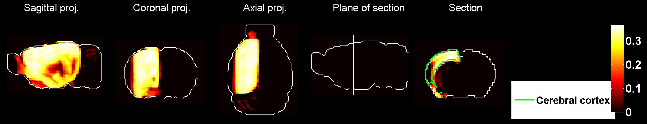
Figure 35: Heat map of the mean correlation profile for cell type labeled $8$.

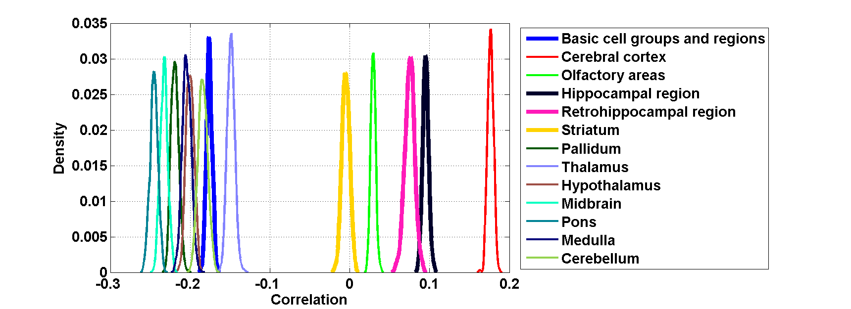
Figure 36: Distribution profiles of the correlations between transcriptome profile of cell type labeled $8$ across random sets of ISH expression energy profiles.

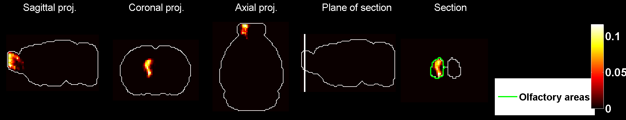
Figure 37: Heat map of the mean density profile for cell type labeled $8$.

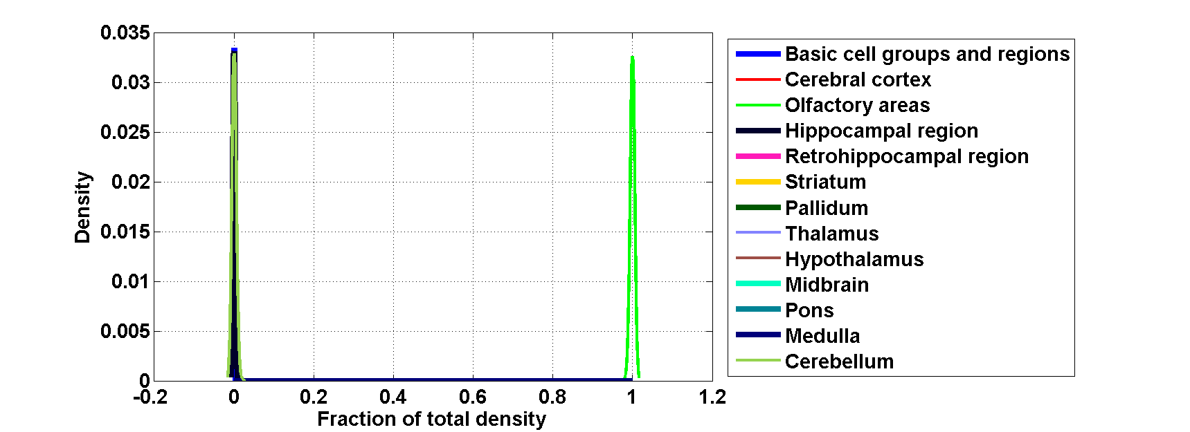
Figure 38: Distribution profiles of the density profile of cell type labeled $8$ across random sets of ISH expression energy profiles.

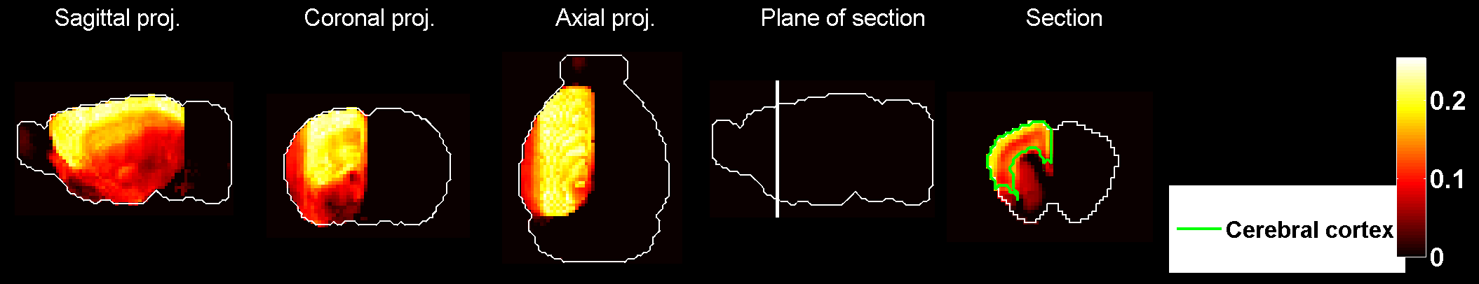
Figure 39: Heat map of the mean correlation profile for cell type labeled $9$.

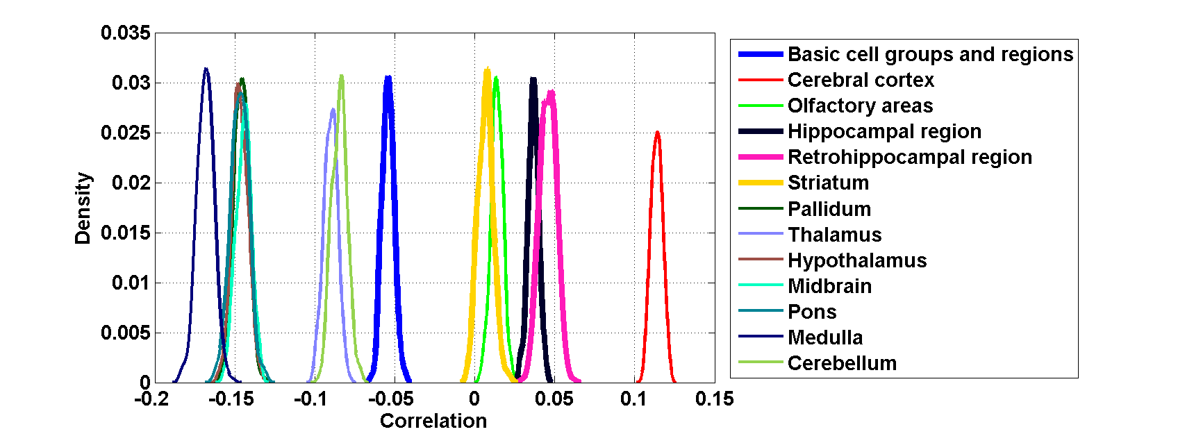
Figure 40: Distribution profiles of the correlations between transcriptome profile of cell type labeled $9$ across random sets of ISH expression energy profiles.

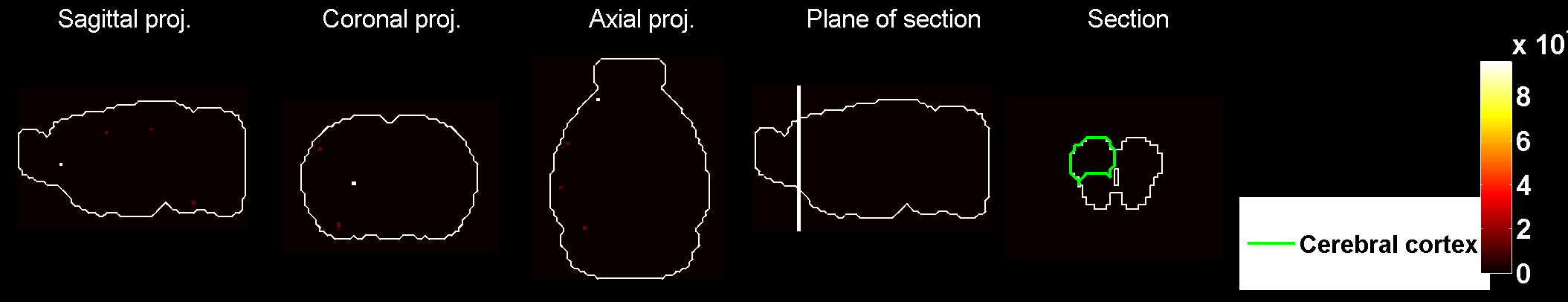
Figure 41: Heat map of the mean density profile for cell type labeled $9$.

Figure 42: Distribution profiles of the density profile of cell type labeled $9$ across random sets of ISH expression energy profiles.

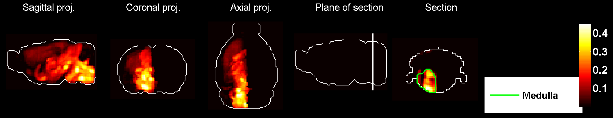
Figure 43: Heat map of the mean correlation profile for cell type labeled $10$.

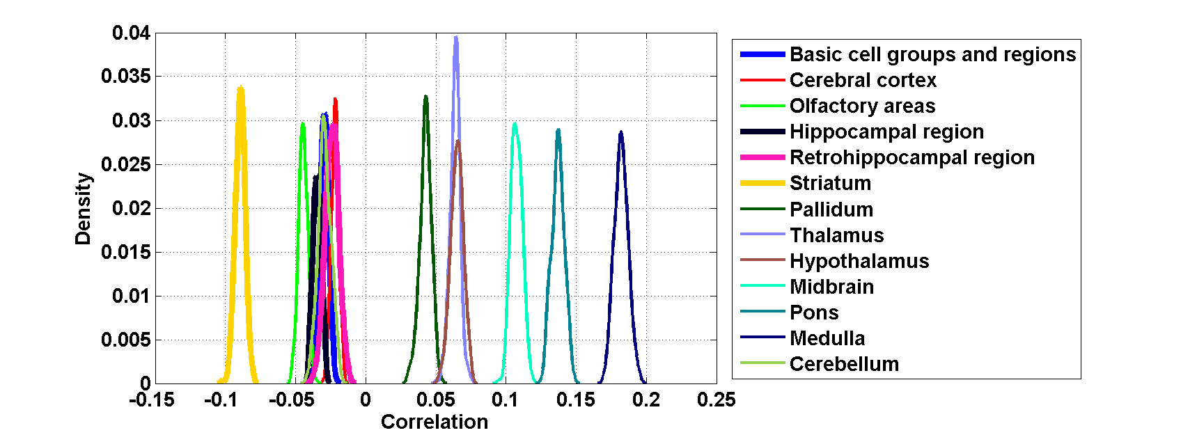
Figure 44: Distribution profiles of the correlations between transcriptome profile of cell type labeled $10$ across random sets of ISH expression energy profiles.

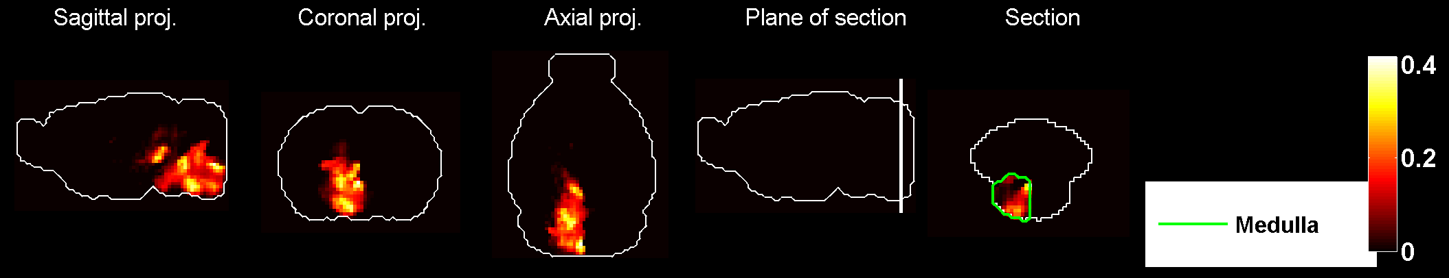
Figure 45: Heat map of the mean density profile for cell type labeled $10$.

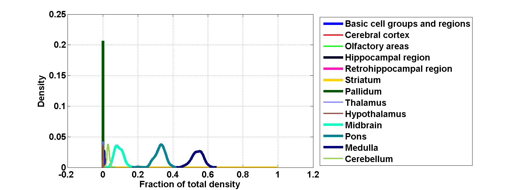
Figure 46: Distribution profiles of the density profile of cell type labeled $10$ across random sets of ISH expression energy profiles.

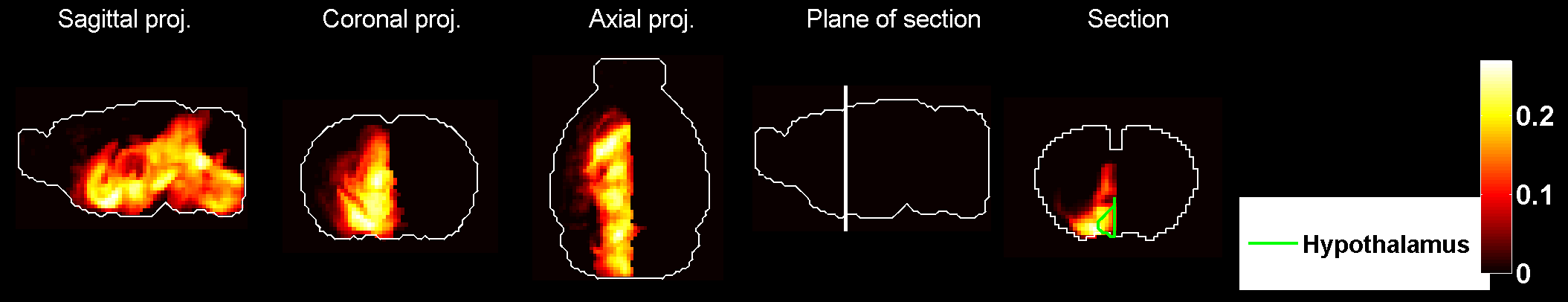
Figure 47: Heat map of the mean correlation profile for cell type labeled $11$.

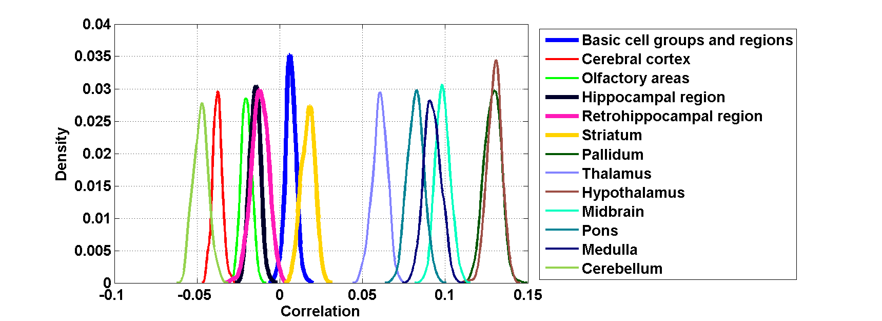
Figure 48: Distribution profiles of the correlations between transcriptome profile of cell type labeled $11$ across random sets of ISH expression energy profiles.

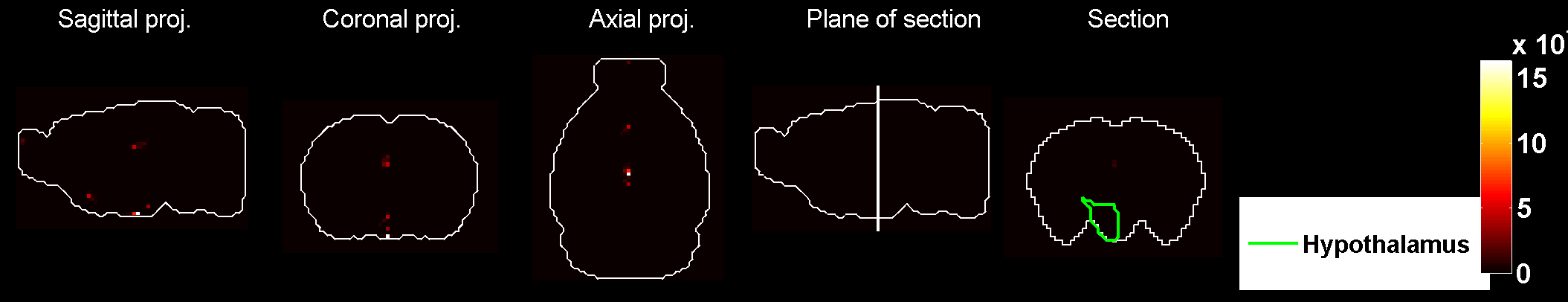
Figure 49: Heat map of the mean density profile for cell type labeled $11$.

Figure 50: Distribution profiles of the density profile of cell type labeled $11$ across random sets of ISH expression energy profiles.

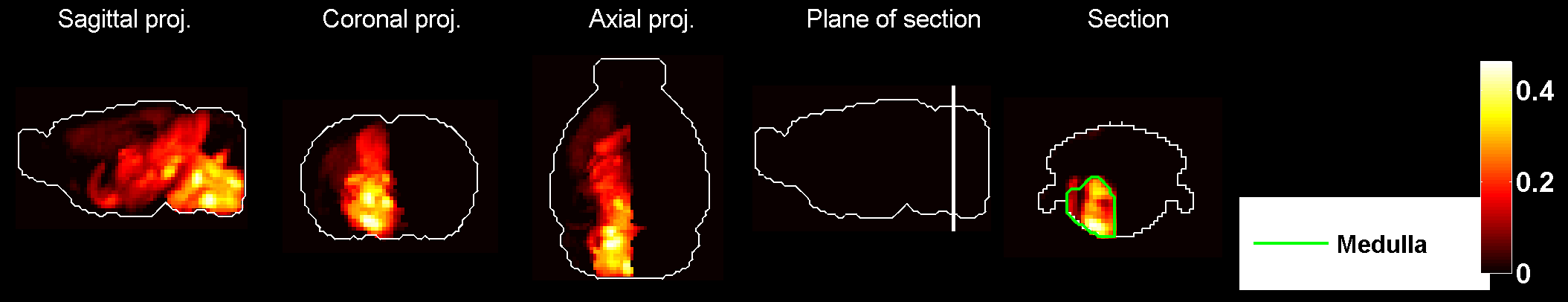
Figure 51: Heat map of the mean correlation profile for cell type labeled $12$.

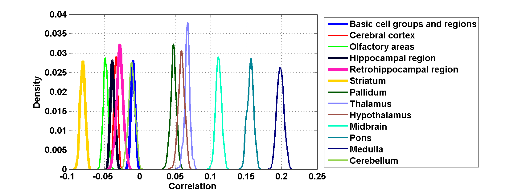
Figure 52: Distribution profiles of the correlations between transcriptome profile of cell type labeled $12$ across random sets of ISH expression energy profiles.

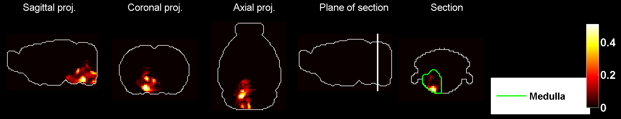
Figure 53: Heat map of the mean density profile for cell type labeled $12$.

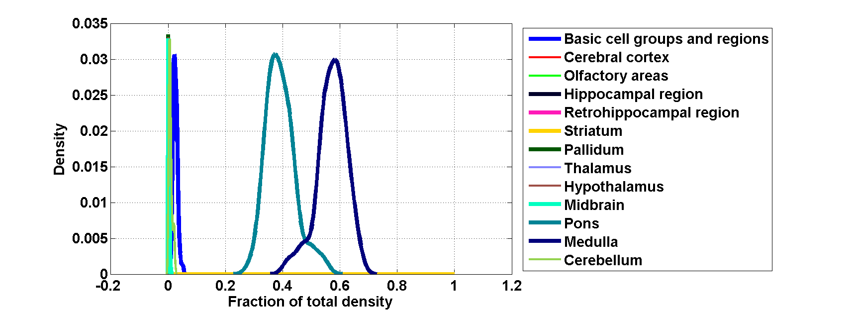
Figure 54: Distribution profiles of the density profile of cell type labeled $12$ across random sets of ISH expression energy profiles.

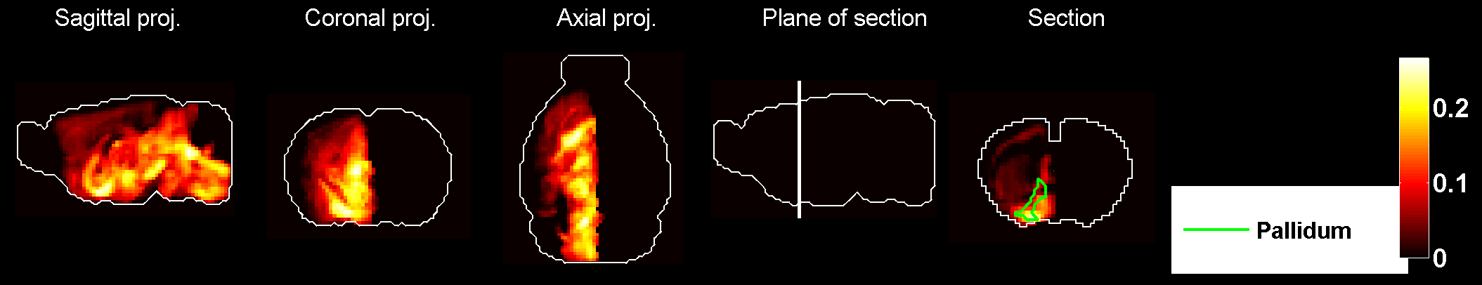
Figure 55: Heat map of the mean correlation profile for cell type labeled $13$.

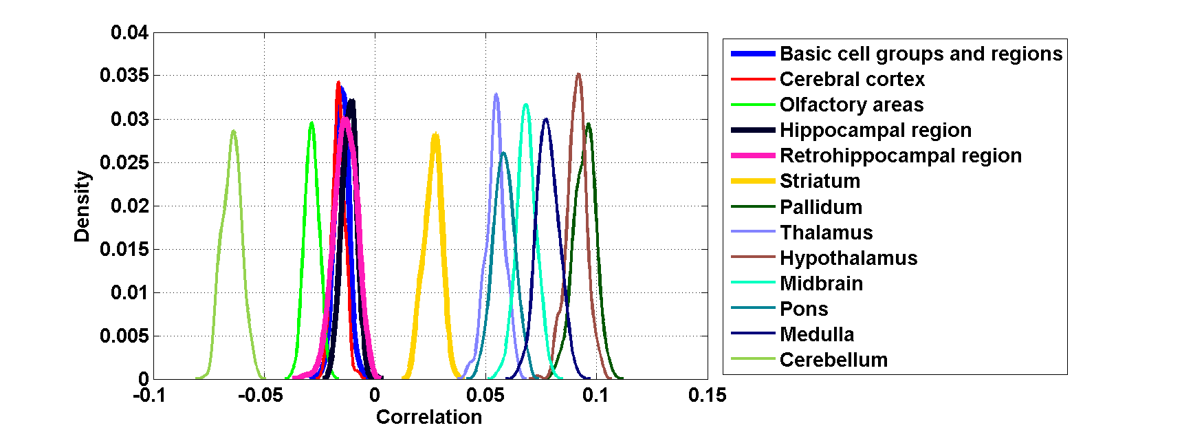
Figure 56: Distribution profiles of the correlations between transcriptome profile of cell type labeled $13$ across random sets of ISH expression energy profiles.

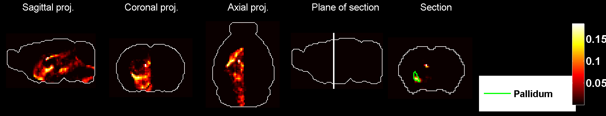
Figure 57: Heat map of the mean density profile for cell type labeled $13$.

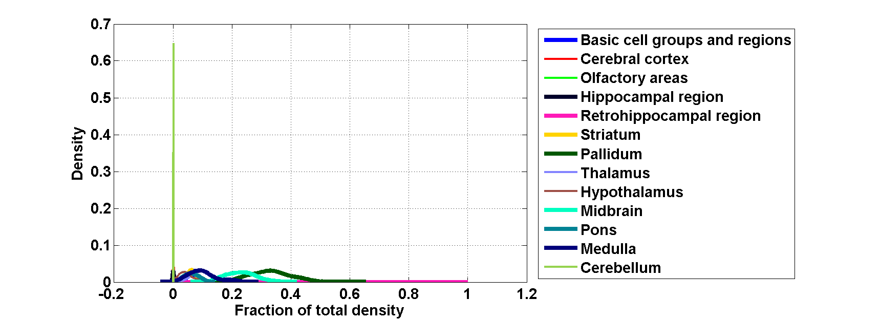
Figure 58: Distribution profiles of the density profile of cell type labeled $13$ across random sets of ISH expression energy profiles.

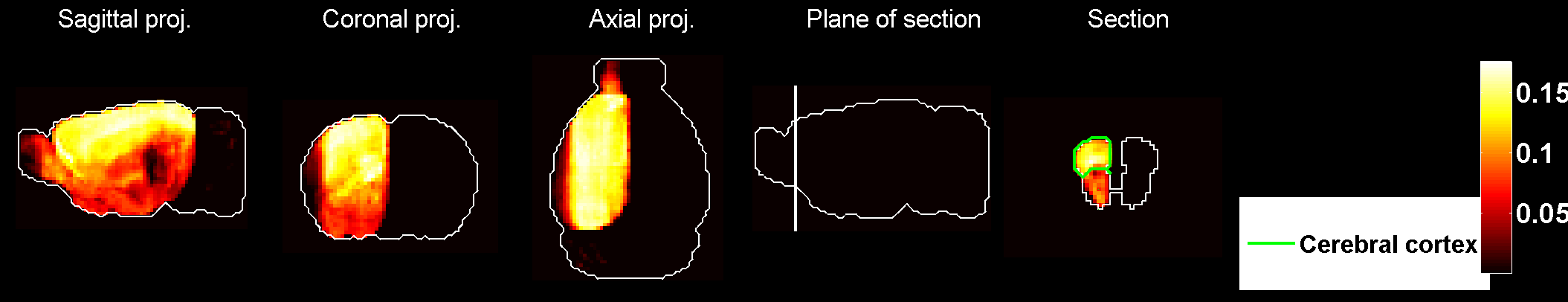
Figure 59: Heat map of the mean correlation profile for cell type labeled $14$.

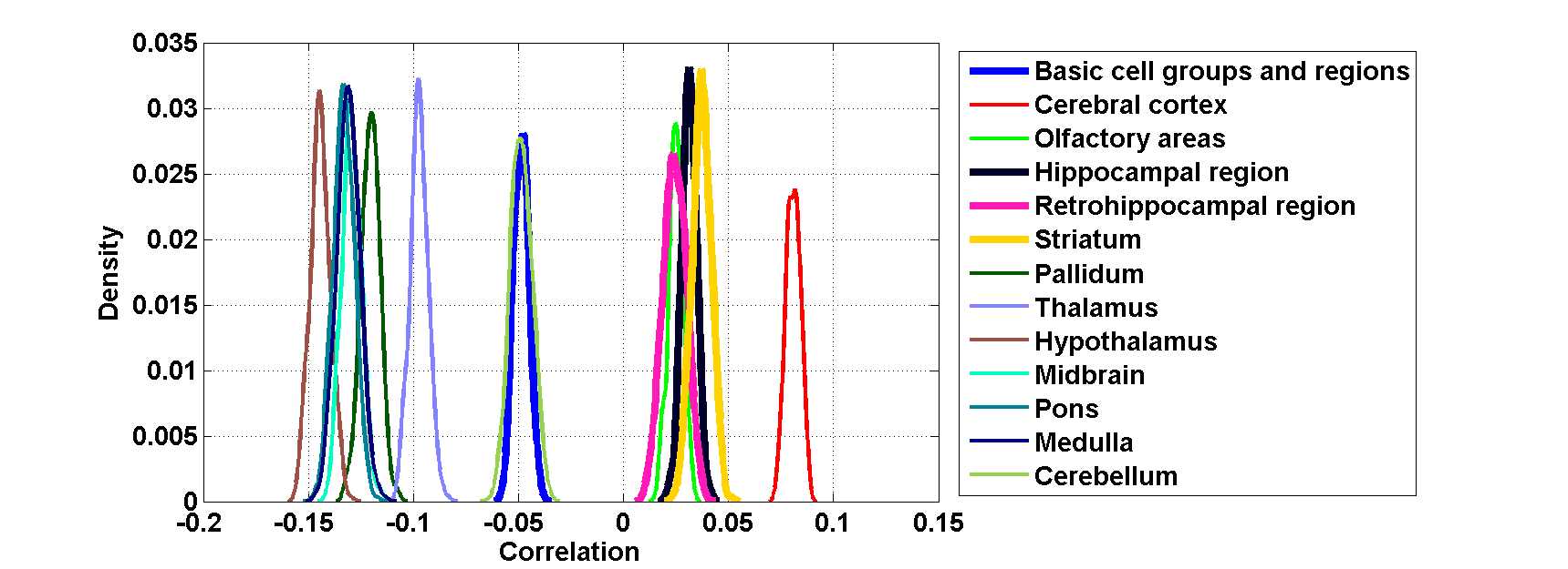
Figure 60: Distribution profiles of the correlations between transcriptome profile of cell type labeled $14$ across random sets of ISH expression energy profiles.

Figure 61: Heat map of the mean density profile for cell type labeled $14$.

Figure 62: Distribution profiles of the density profile of cell type labeled $14$ across random sets of ISH expression energy profiles.

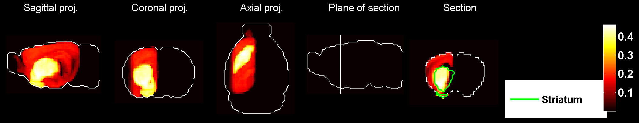
Figure 63: Heat map of the mean correlation profile for cell type labeled $15$.

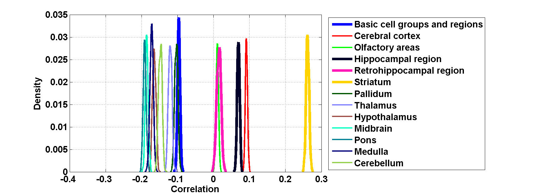
Figure 64: Distribution profiles of the correlations between transcriptome profile of cell type labeled $15$ across random sets of ISH expression energy profiles.

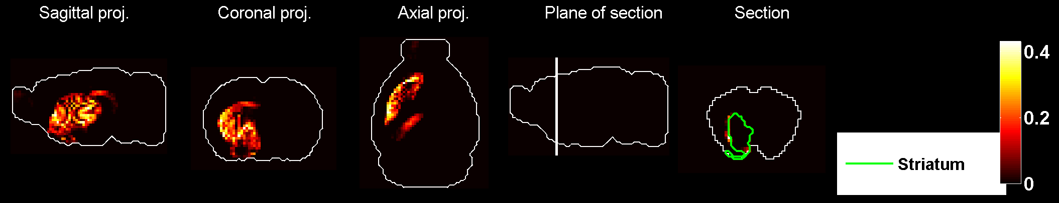
Figure 65: Heat map of the mean density profile for cell type labeled $15$.

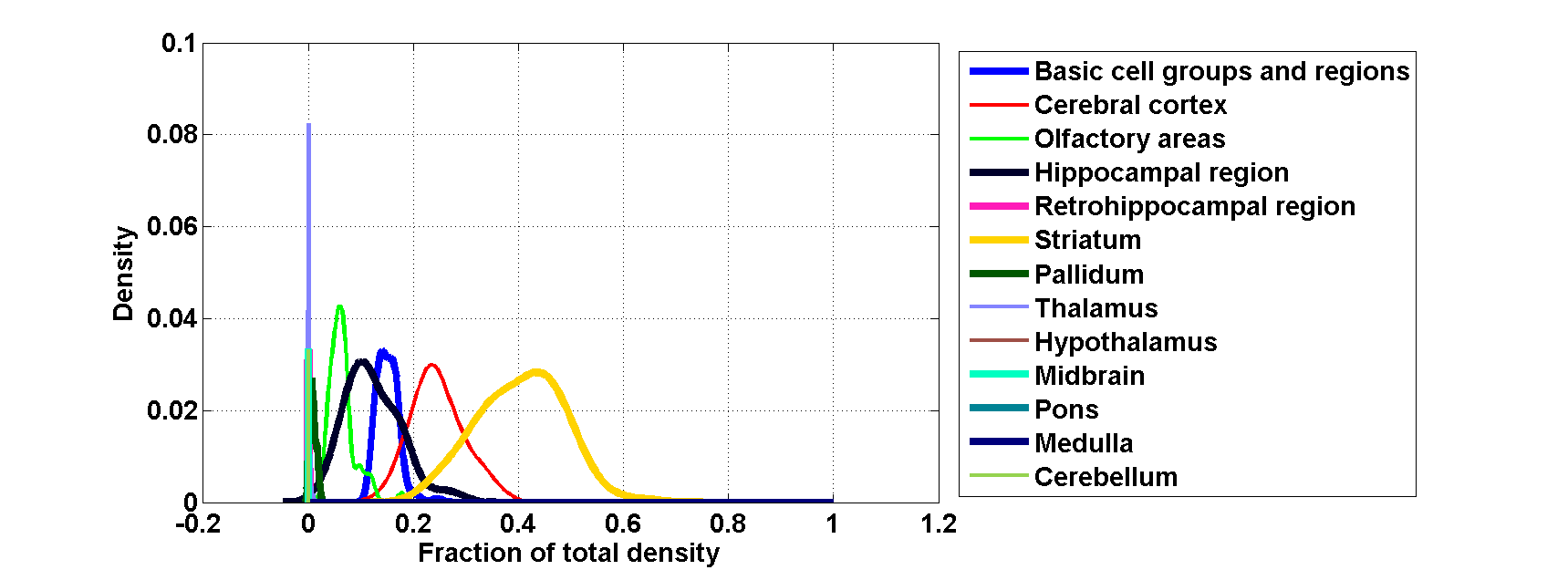
Figure 66: Distribution profiles of the density profile of cell type labeled $15$ across random sets of ISH expression energy profiles.

Figure 67: Heat map of the mean correlation profile for cell type labeled $16$.

Figure 68: Distribution profiles of the correlations between transcriptome profile of cell type labeled $16$ across random sets of ISH expression energy profiles.

Figure 69: Heat map of the mean density profile for cell type labeled $16$.

Figure 70: Distribution profiles of the density profile of cell type labeled $16$ across random sets of ISH expression energy profiles.

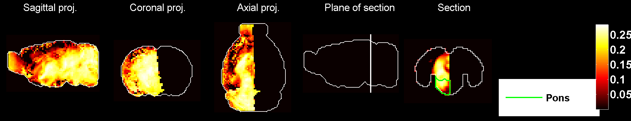
Figure 71: Heat map of the mean correlation profile for cell type labeled $17$.

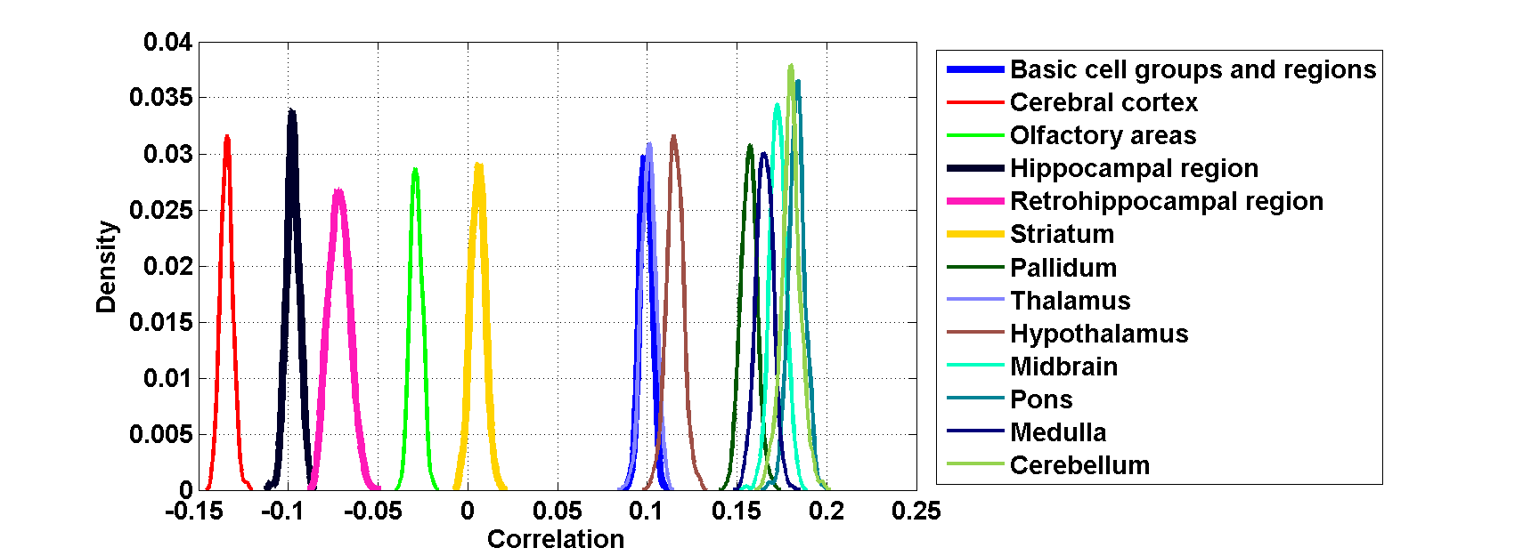
Figure 72: Distribution profiles of the correlations between transcriptome profile of cell type labeled $17$ across random sets of ISH expression energy profiles.

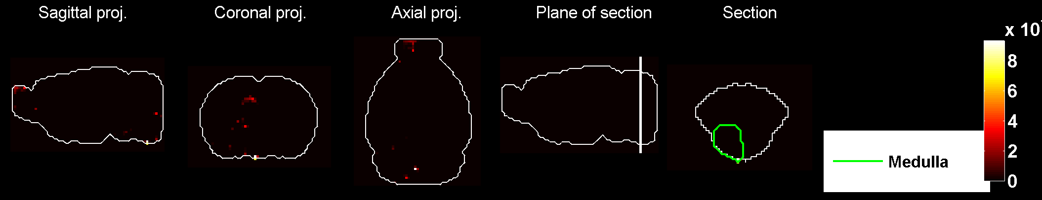
Figure 73: Heat map of the mean density profile for cell type labeled $17$.

Figure 74: Distribution profiles of the density profile of cell type labeled $17$ across random sets of ISH expression energy profiles.

Figure 75: Heat map of the mean correlation profile for cell type labeled $18$.

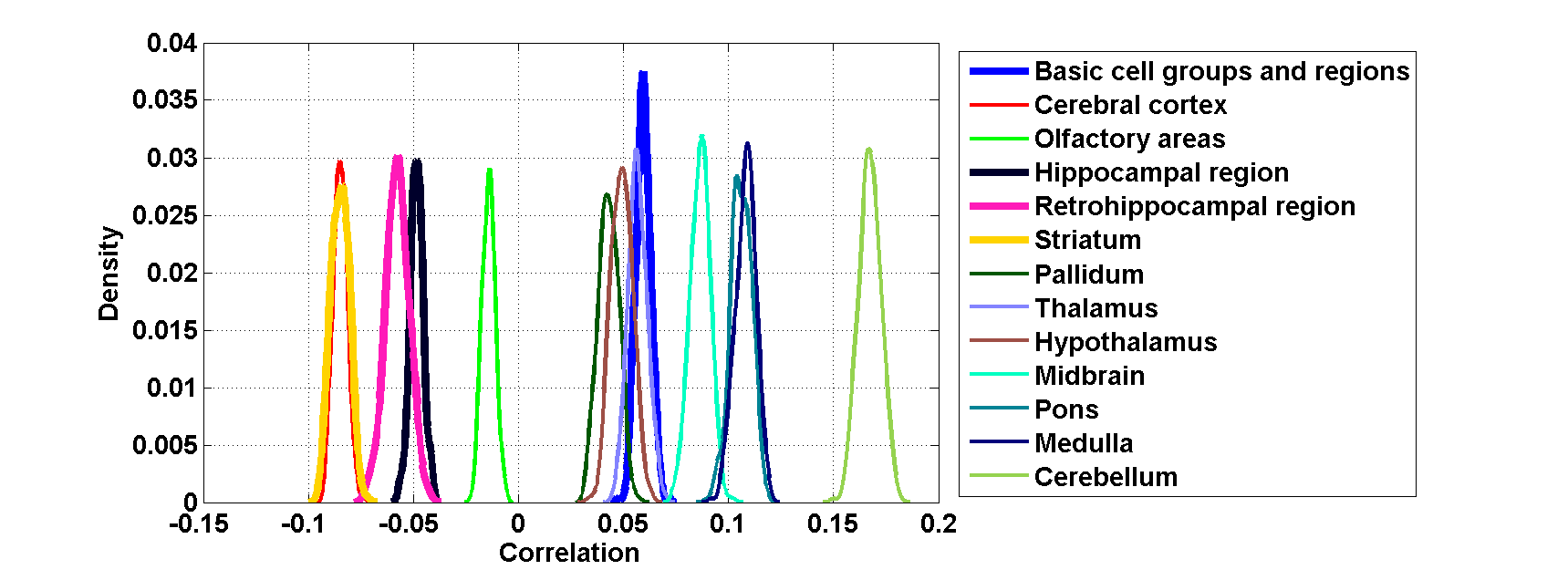
Figure 76: Distribution profiles of the correlations between transcriptome profile of cell type labeled $18$ across random sets of ISH expression energy profiles.

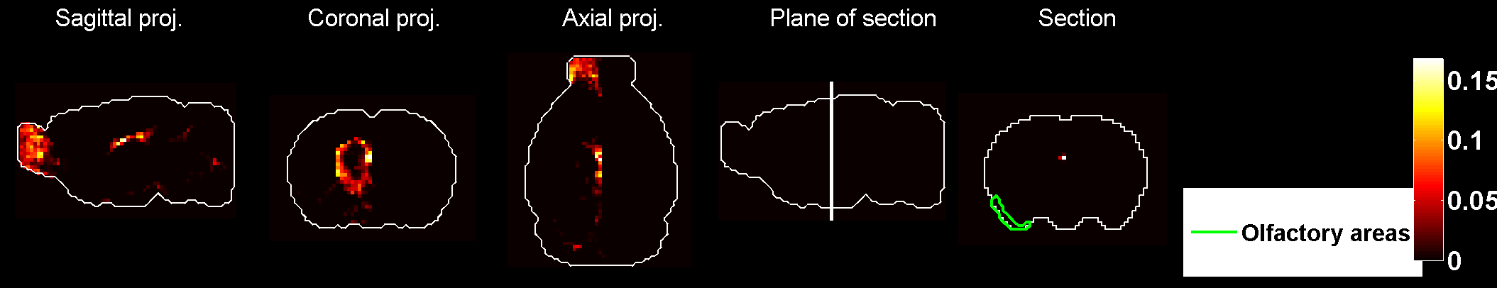
Figure 77: Heat map of the mean density profile for cell type labeled $18$.

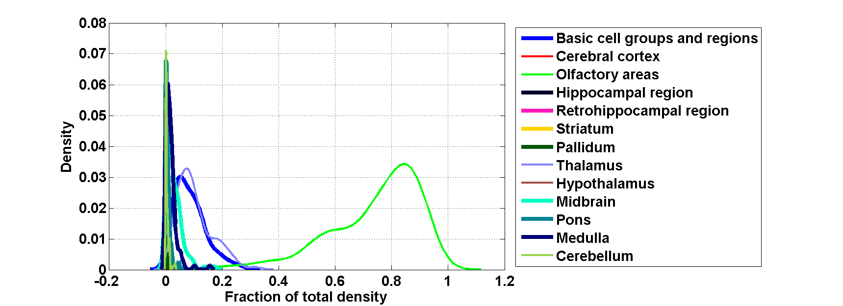
Figure 78: Distribution profiles of the density profile of cell type labeled $18$ across random sets of ISH expression energy profiles.

Figure 79: Heat map of the mean correlation profile for cell type labeled $19$.

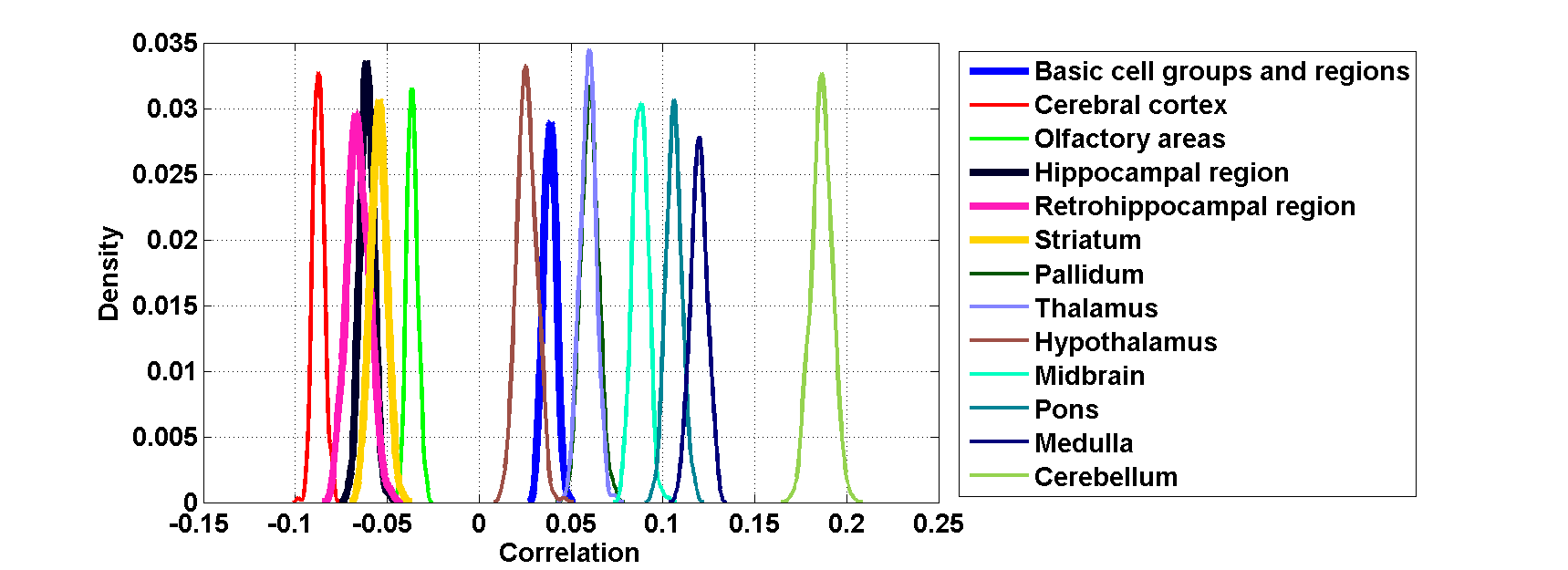
Figure 80: Distribution profiles of the correlations between transcriptome profile of cell type labeled $19$ across random sets of ISH expression energy profiles.

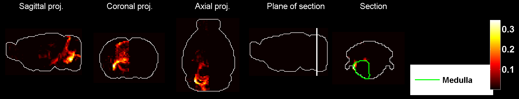
Figure 81: Heat map of the mean density profile for cell type labeled $19$.

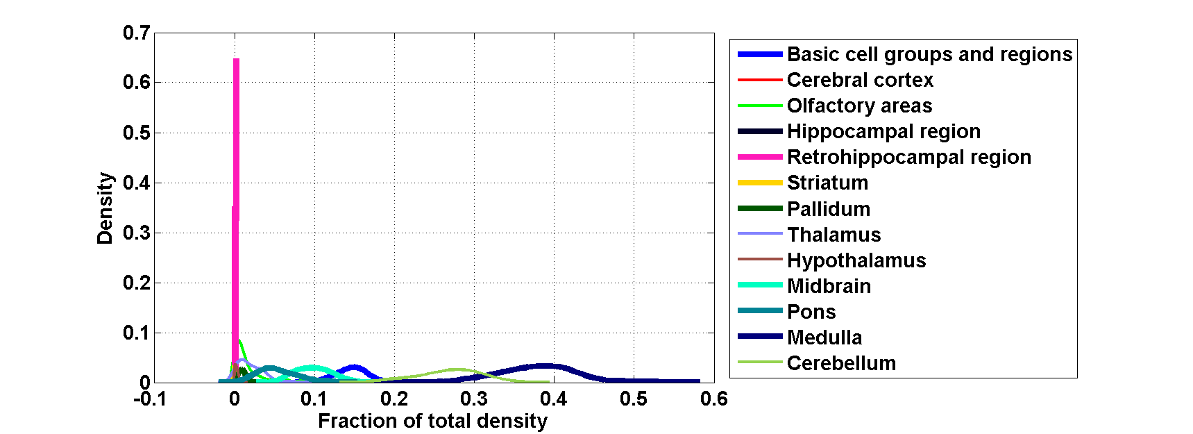
Figure 82: Distribution profiles of the density profile of cell type labeled $19$ across random sets of ISH expression energy profiles.

Figure 83: Heat map of the mean correlation profile for cell type labeled $20$.

Figure 84: Distribution profiles of the correlations between transcriptome profile of cell type labeled $20$ across random sets of ISH expression energy profiles.

Figure 85: Heat map of the mean density profile for cell type labeled $20$.

Figure 86: Distribution profiles of the density profile of cell type labeled $20$ across random sets of ISH expression energy profiles.

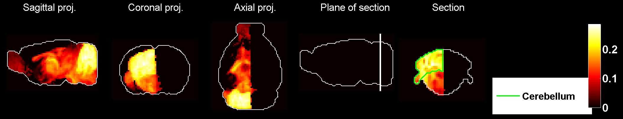
Figure 87: Heat map of the mean correlation profile for cell type labeled $21$.

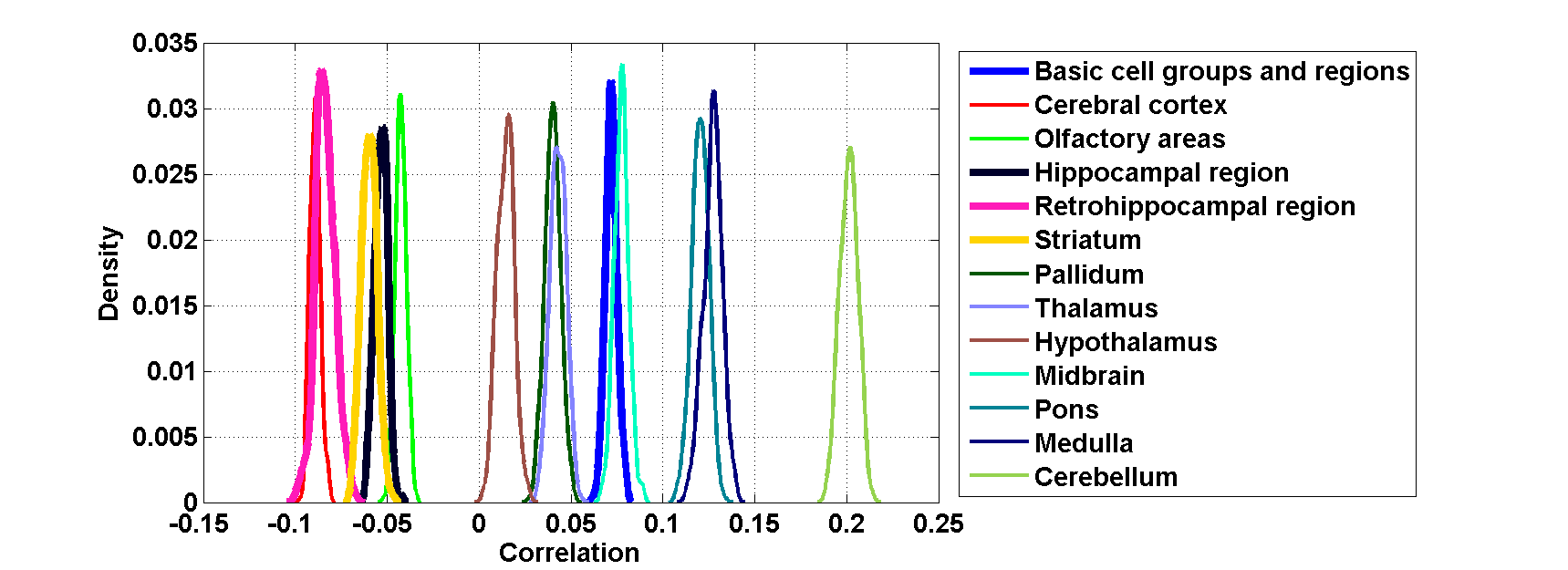
Figure 88: Distribution profiles of the correlations between transcriptome profile of cell type labeled $21$ across random sets of ISH expression energy profiles.

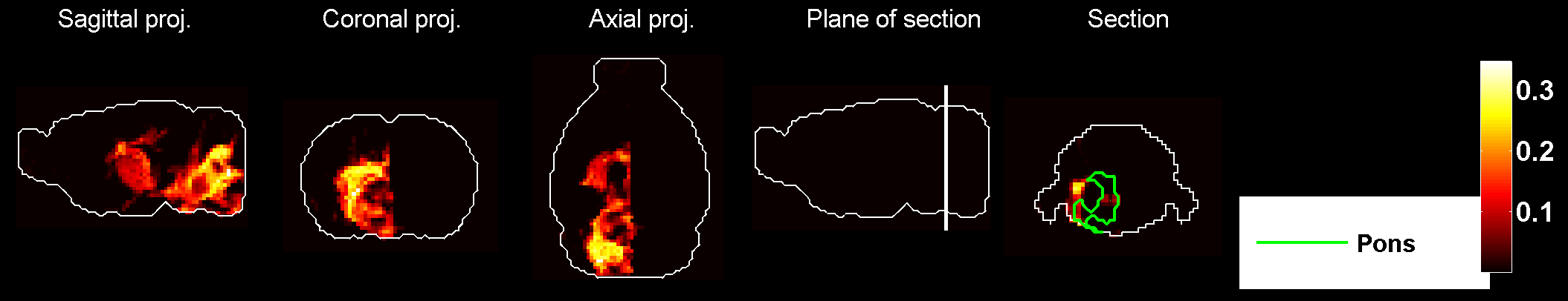
Figure 89: Heat map of the mean density profile for cell type labeled $21$.

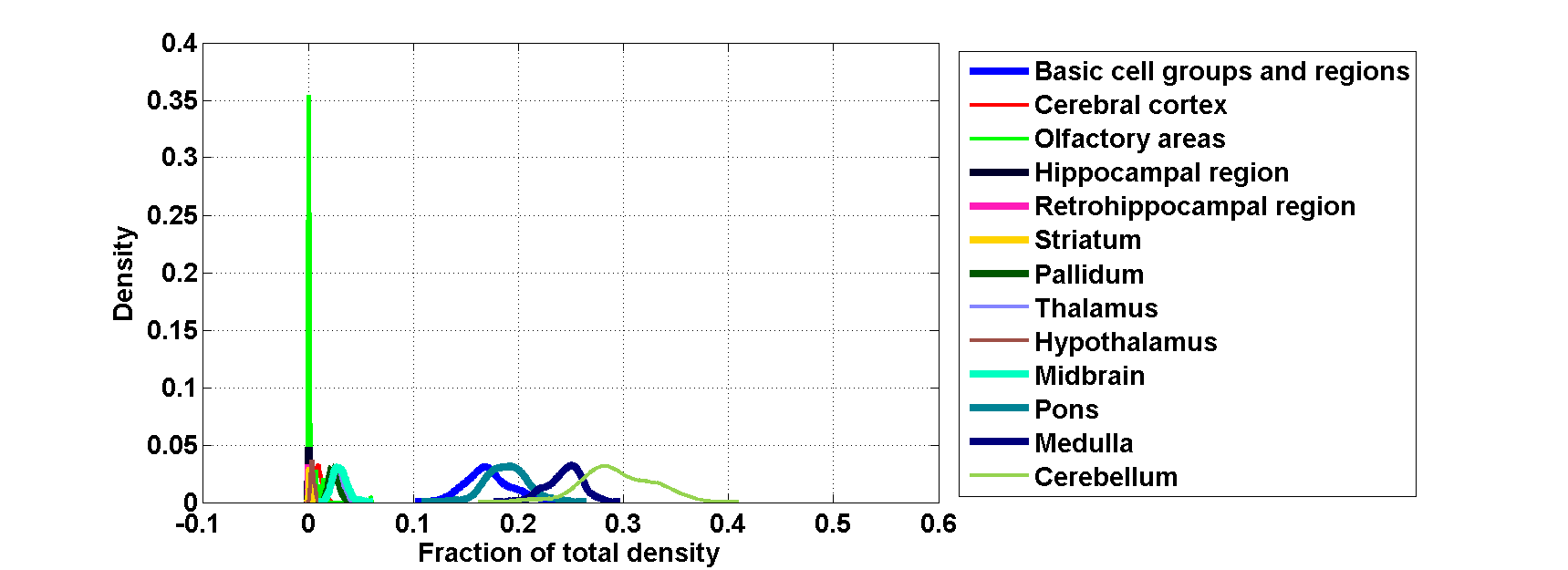
Figure 90: Distribution profiles of the density profile of cell type labeled $21$ across random sets of ISH expression energy profiles.

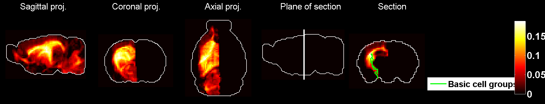
Figure 91: Heat map of the mean correlation profile for cell type labeled $22$.

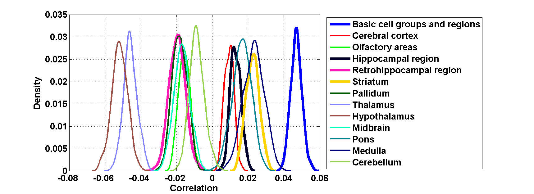
Figure 92: Distribution profiles of the correlations between transcriptome profile of cell type labeled $22$ across random sets of ISH expression energy profiles.

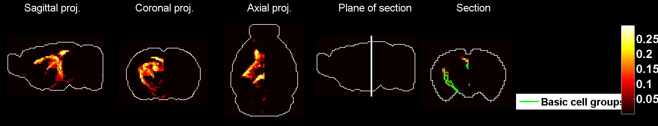
Figure 93: Heat map of the mean density profile for cell type labeled $22$.

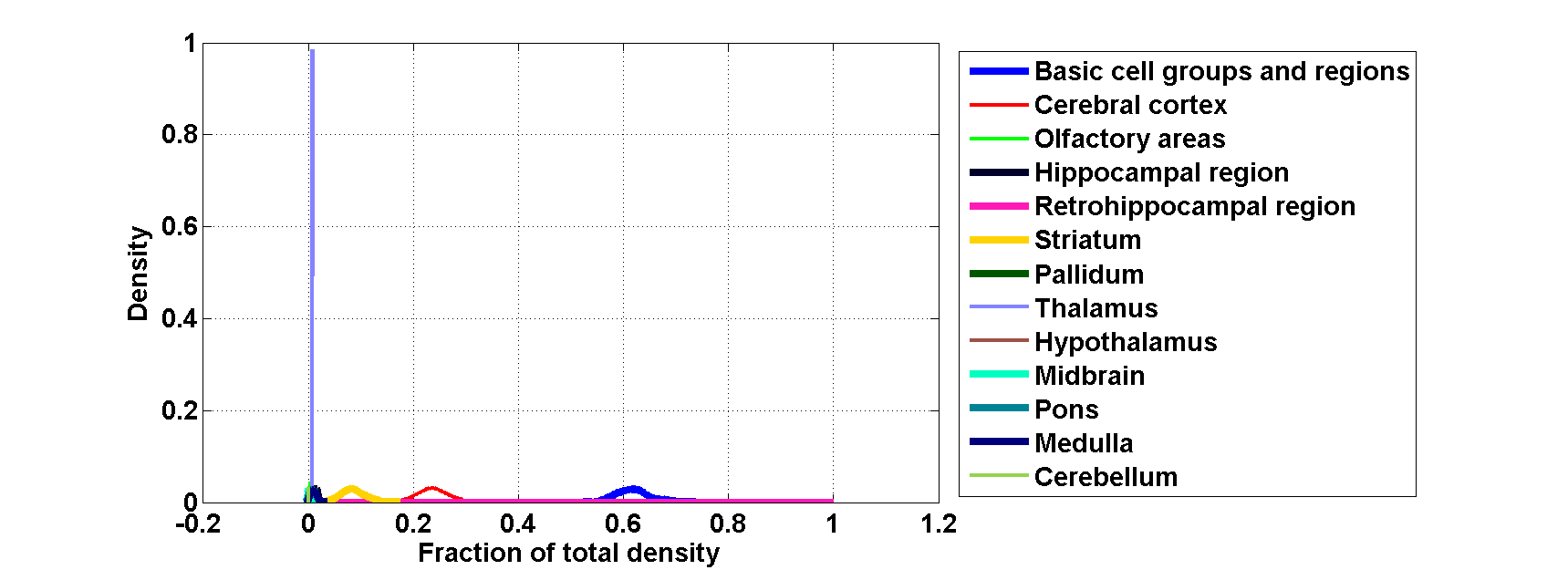
Figure 94: Distribution profiles of the density profile of cell type labeled $22$ across random sets of ISH expression energy profiles.

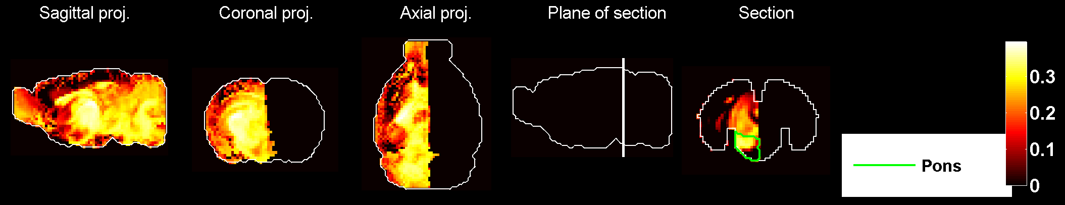
Figure 95: Heat map of the mean correlation profile for cell type labeled $23$.

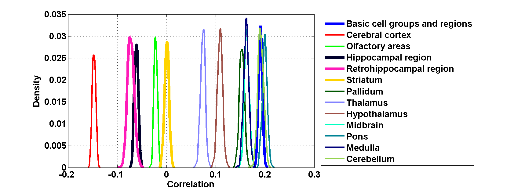
Figure 96: Distribution profiles of the correlations between transcriptome profile of cell type labeled $23$ across random sets of ISH expression energy profiles.

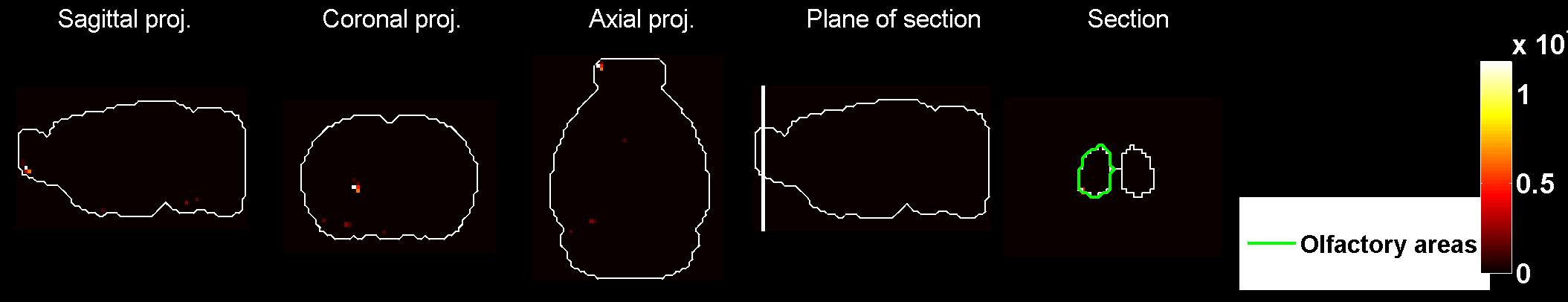
Figure 97: Heat map of the mean density profile for cell type labeled $23$.

Figure 98: Distribution profiles of the density profile of cell type labeled $23$ across random sets of ISH expression energy profiles.

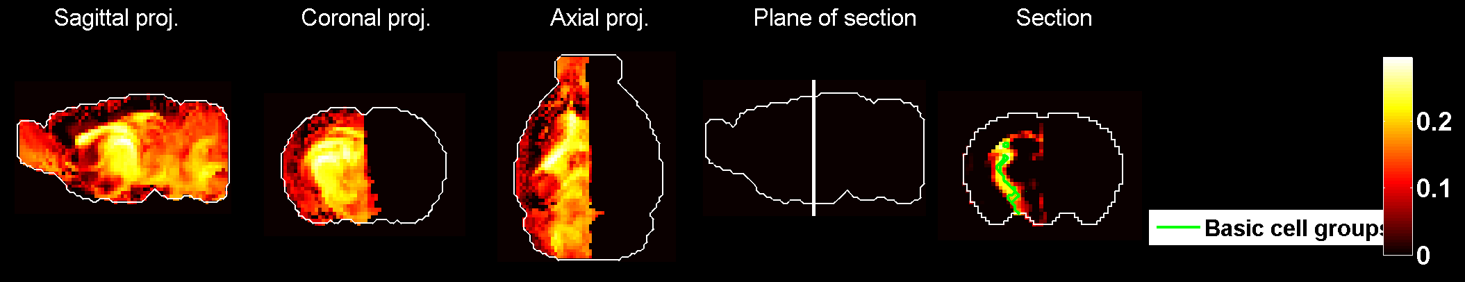
Figure 99: Heat map of the mean correlation profile for cell type labeled $24$.

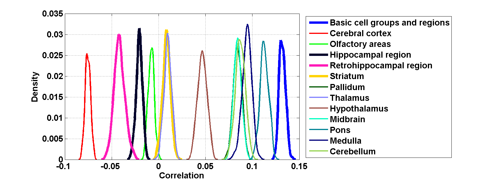
Figure 100: Distribution profiles of the correlations between transcriptome profile of cell type labeled $24$ across random sets of ISH expression energy profiles.

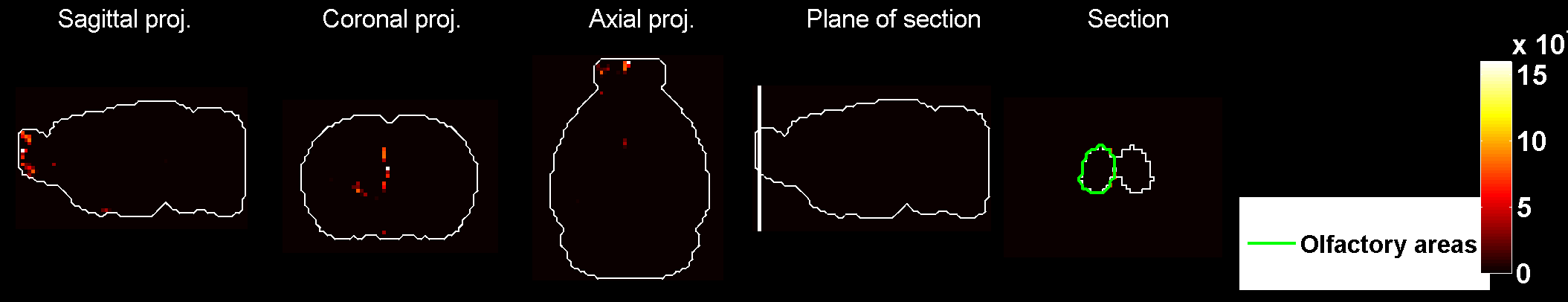
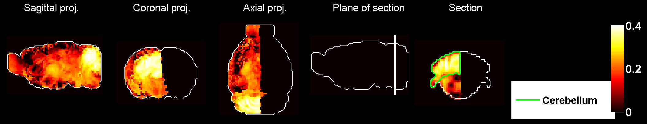
Figure 101: Heat map of the mean density profile for cell type labeled $24$.

Figure 102: Distribution profiles of the density profile of cell type labeled $24$ across random sets of ISH expression energy profiles.

Figure 103: Heat map of the mean correlation profile for cell type labeled $25$.

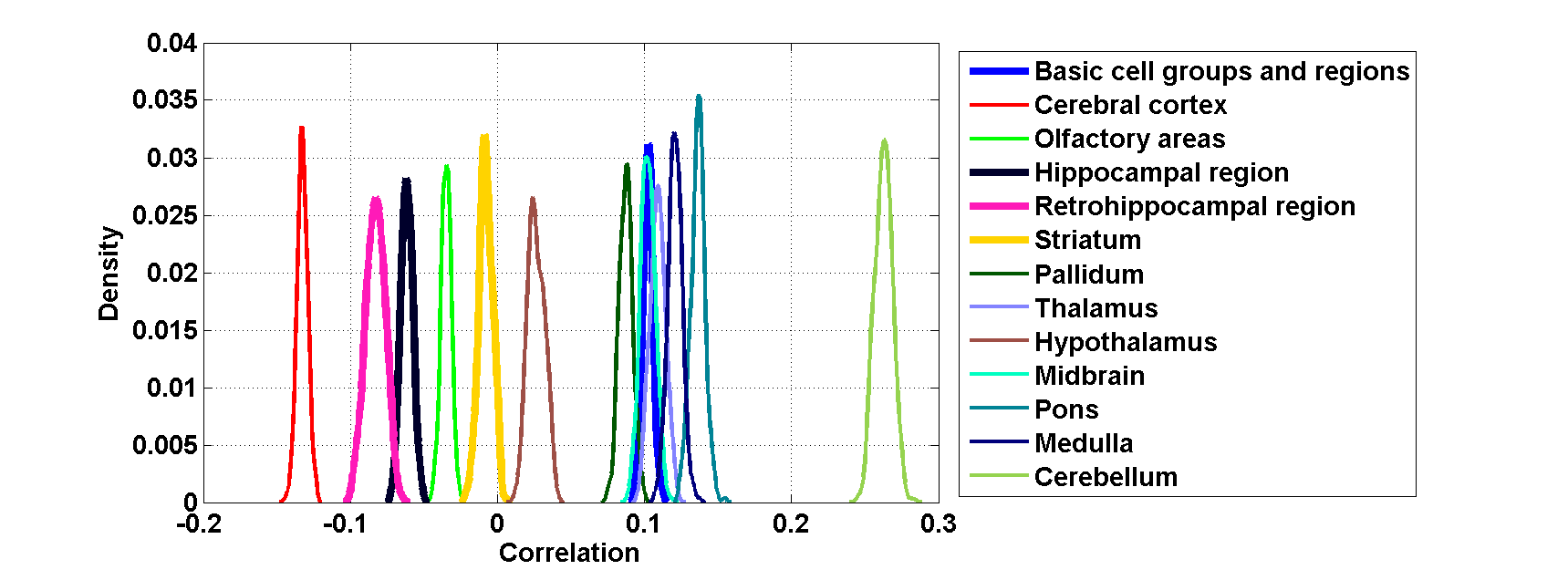
Figure 104: Distribution profiles of the correlations between transcriptome profile of cell type labeled $25$ across random sets of ISH expression energy profiles.

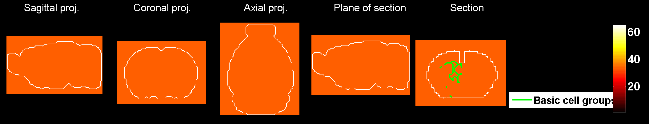
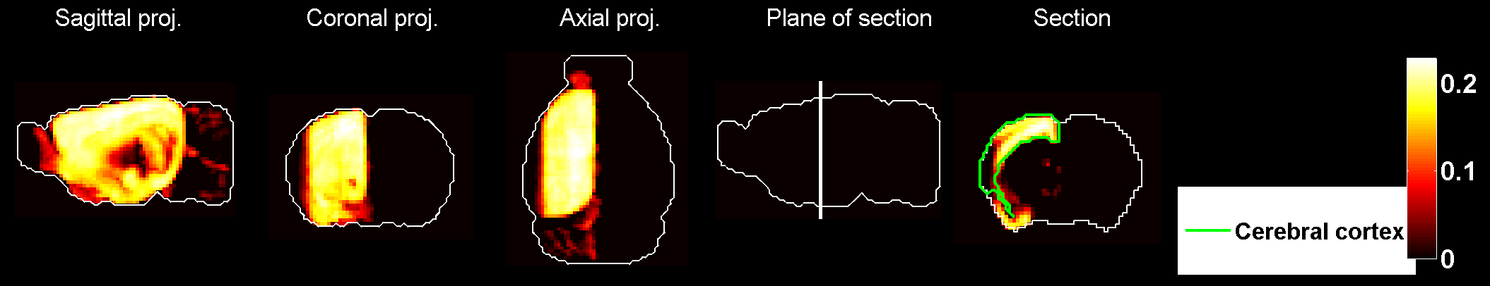
Figure 105: Heat map of the mean density profile for cell type labeled $25$.

Figure 106: Distribution profiles of the density profile of cell type labeled $25$ across random sets of ISH expression energy profiles.

Figure 107: Heat map of the mean correlation profile for cell type labeled $26$.

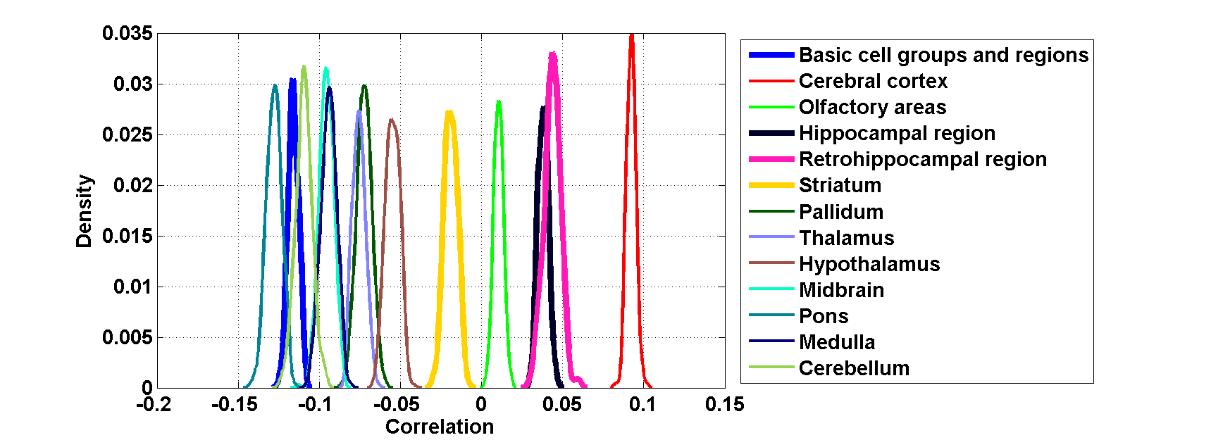
Figure 108: Distribution profiles of the correlations between transcriptome profile of cell type labeled $26$ across random sets of ISH expression energy profiles.

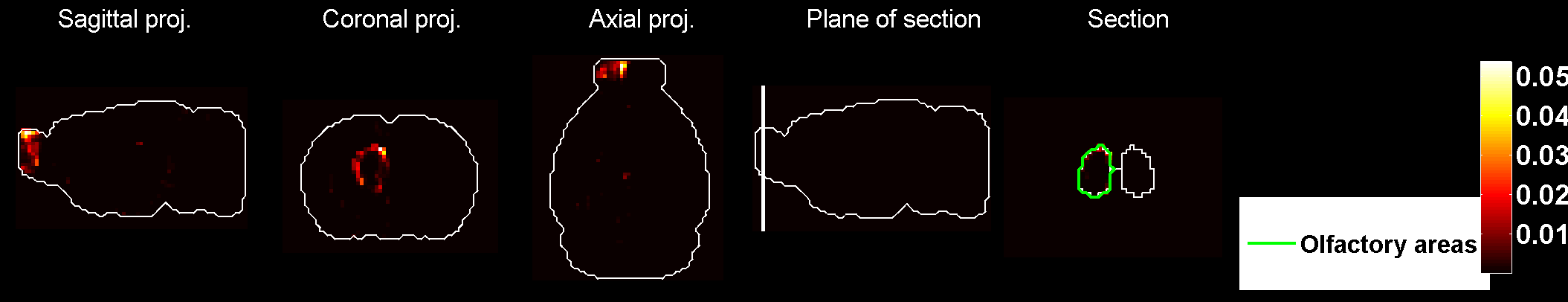
Figure 109: Heat map of the mean density profile for cell type labeled $26$.

Figure 110: Distribution profiles of the density profile of cell type labeled $26$ across random sets of ISH expression energy profiles.

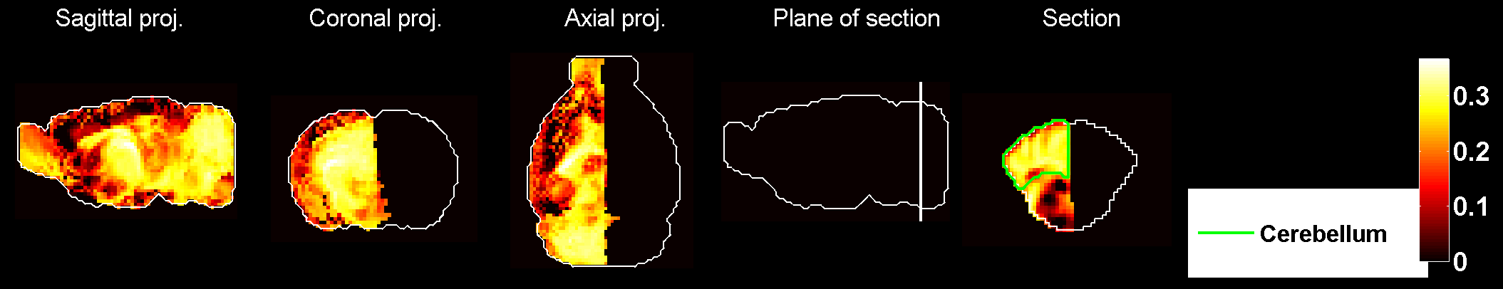
Figure 111: Heat map of the mean correlation profile for cell type labeled $27$.

Figure 112: Distribution profiles of the correlations between transcriptome profile of cell type labeled $27$ across random sets of ISH expression energy profiles.

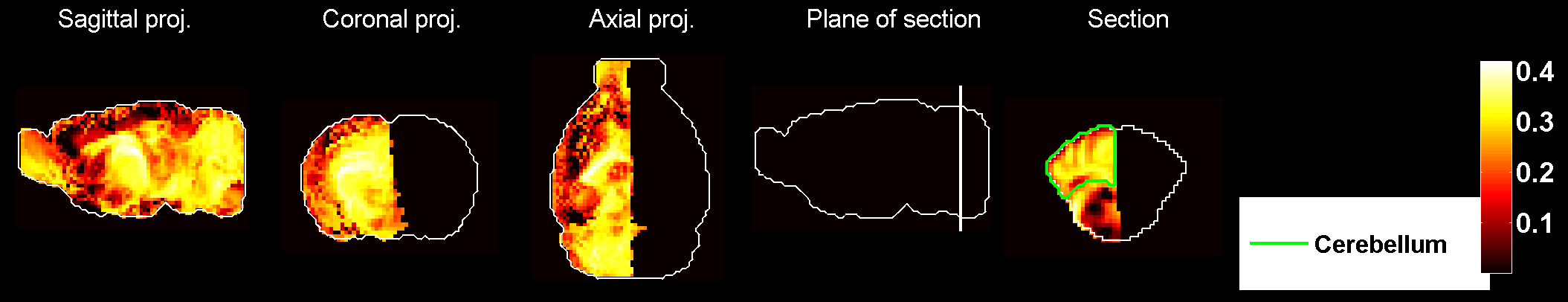
Figure 113: Heat map of the mean density profile for cell type labeled $27$.

Figure 114: Distribution profiles of the density profile of cell type labeled $27$ across random sets of ISH expression energy profiles.

Figure 115: Heat map of the mean correlation profile for cell type labeled $28$.

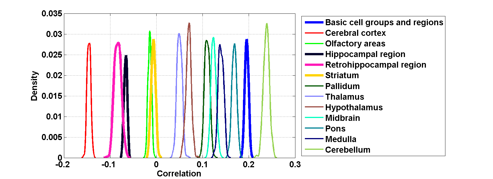
Figure 116: Distribution profiles of the correlations between transcriptome profile of cell type labeled $28$ across random sets of ISH expression energy profiles.

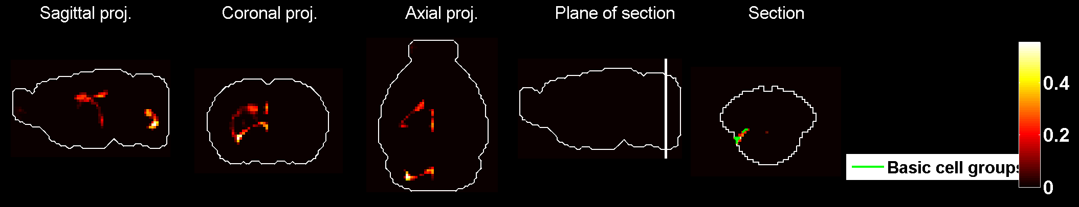
Figure 117: Heat map of the mean density profile for cell type labeled $28$.

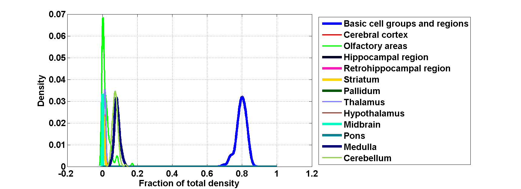
Figure 118: Distribution profiles of the density profile of cell type labeled $28$ across random sets of ISH expression energy profiles.

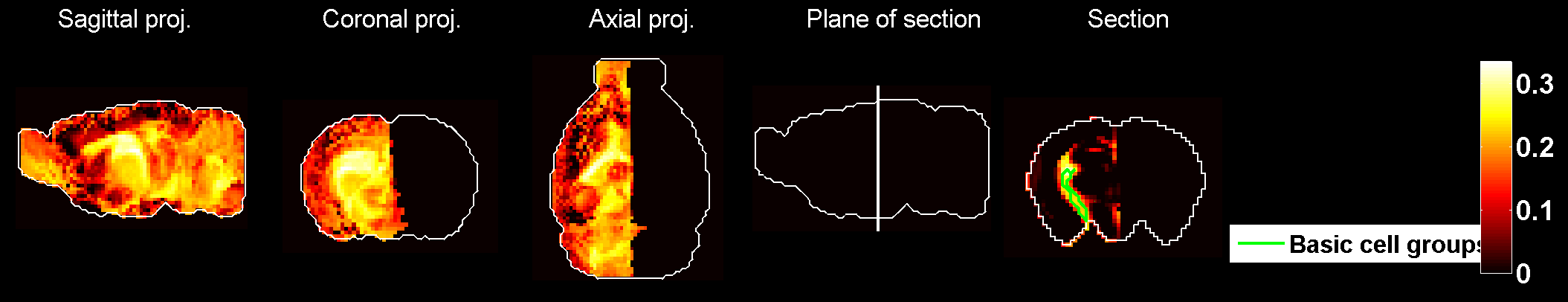
Figure 119: Heat map of the mean correlation profile for cell type labeled $29$.

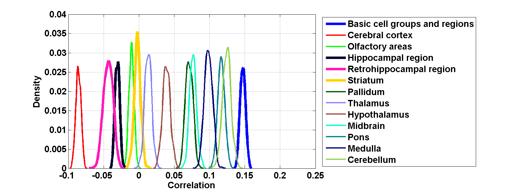
Figure 120: Distribution profiles of the correlations between transcriptome profile of cell type labeled $29$ across random sets of ISH expression energy profiles.

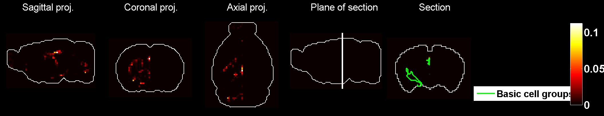
Figure 121: Heat map of the mean density profile for cell type labeled $29$.

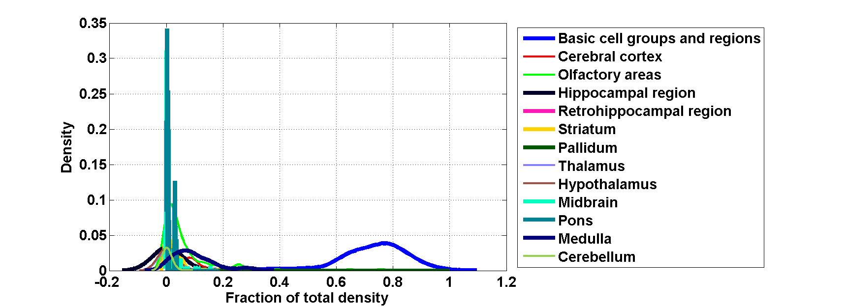
Figure 122: Distribution profiles of the density profile of cell type labeled $29$ across random sets of ISH expression energy profiles.

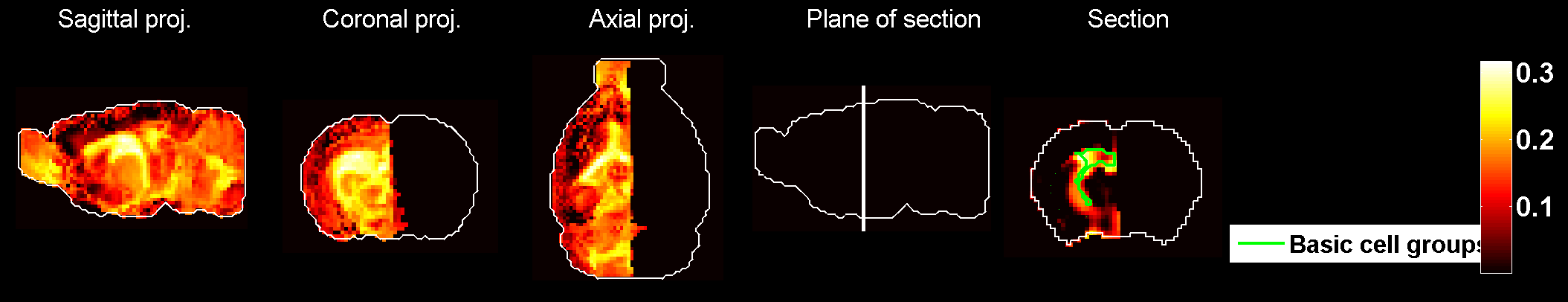
Figure 123: Heat map of the mean correlation profile for cell type labeled $30$.

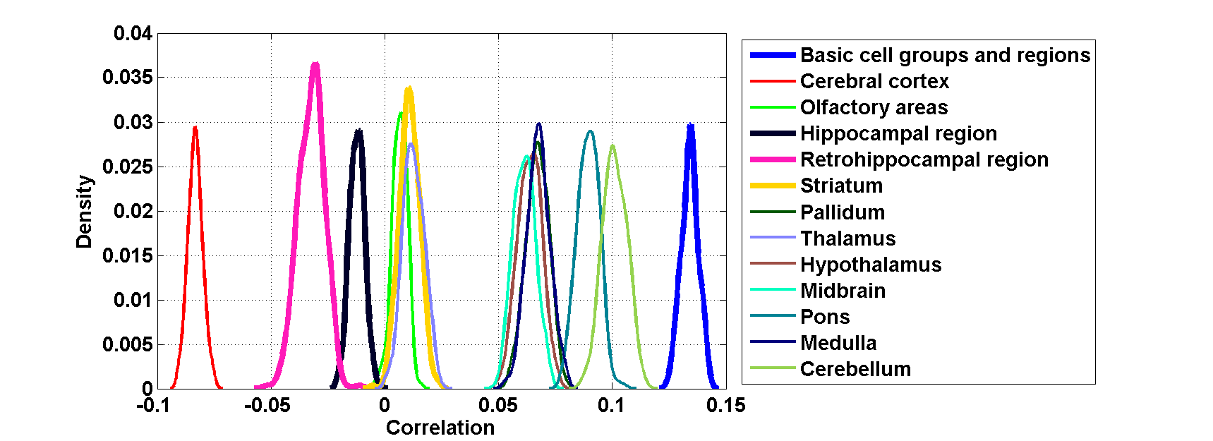
Figure 124: Distribution profiles of the correlations between transcriptome profile of cell type labeled $30$ across random sets of ISH expression energy profiles.

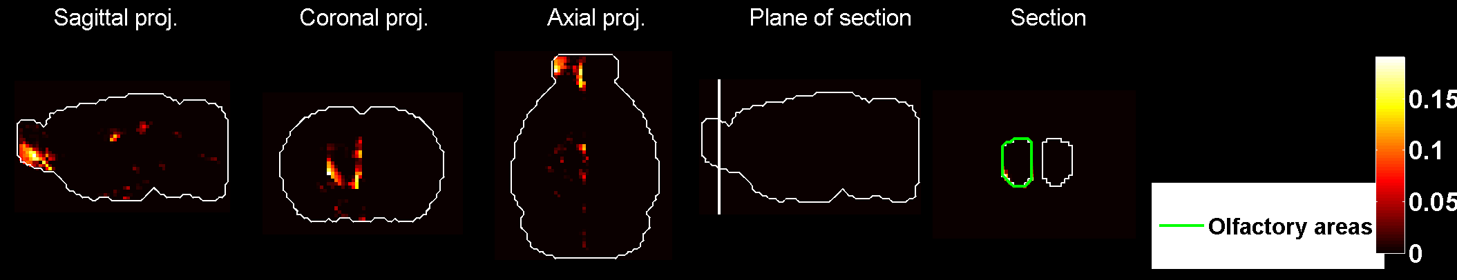
Figure 125: Heat map of the mean density profile for cell type labeled $30$.

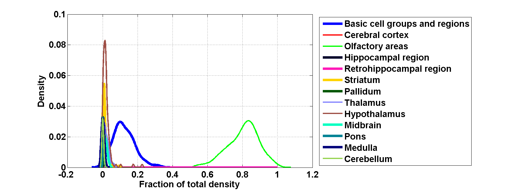
Figure 126: Distribution profiles of the density profile of cell type labeled $30$ across random sets of ISH expression energy profiles.

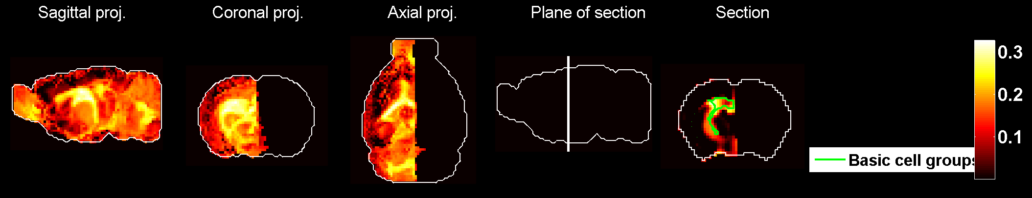
Figure 127: Heat map of the mean correlation profile for cell type labeled $31$.

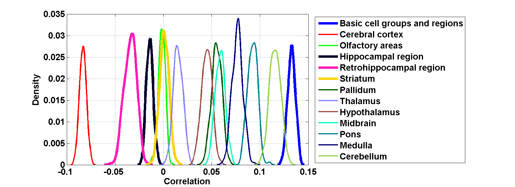
Figure 128: Distribution profiles of the correlations between transcriptome profile of cell type labeled $31$ across random sets of ISH expression energy profiles.

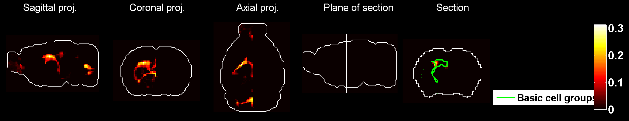
Figure 129: Heat map of the mean density profile for cell type labeled $31$.

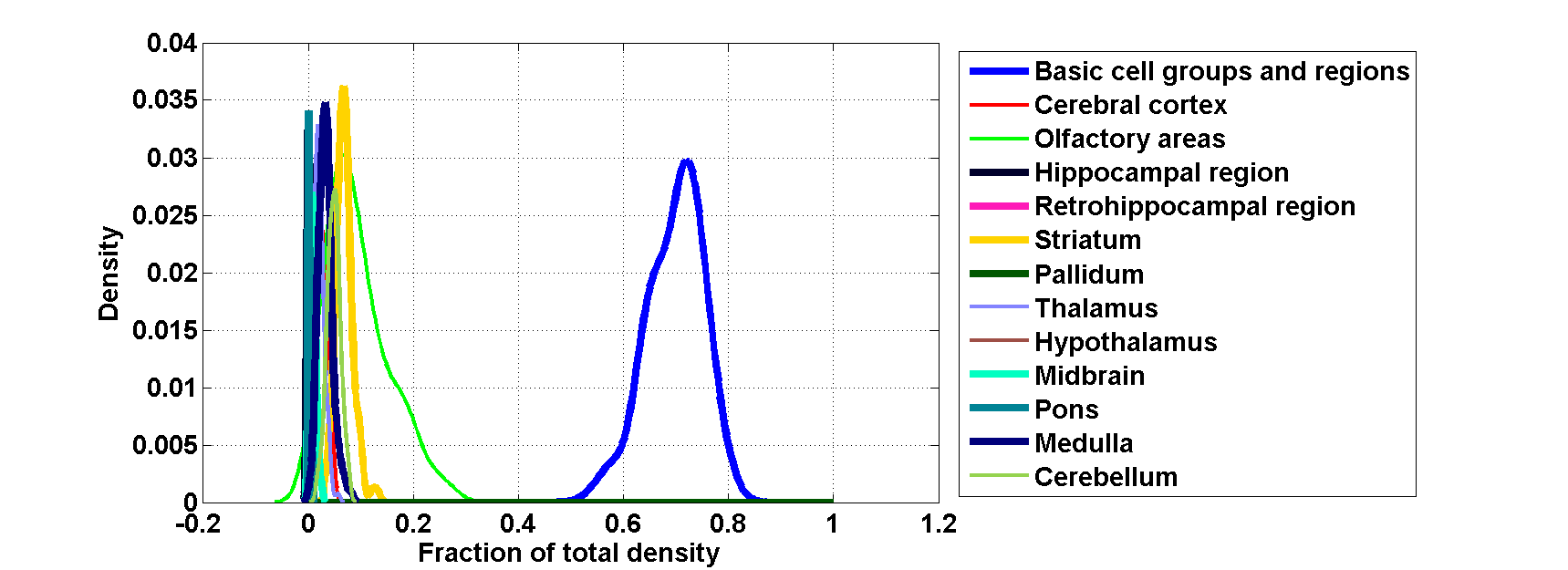
Figure 130: Distribution profiles of the density profile of cell type labeled $31$ across random sets of ISH expression energy profiles.

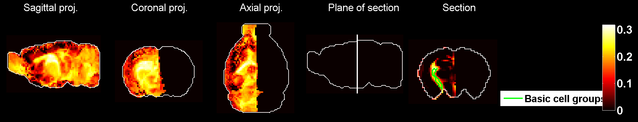
Figure 131: Heat map of the mean correlation profile for cell type labeled $32$.

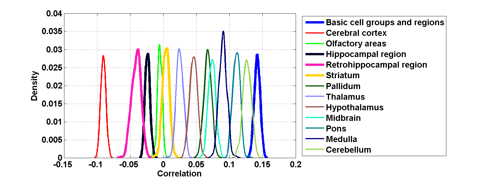
Figure 132: Distribution profiles of the correlations between transcriptome profile of cell type labeled $32$ across random sets of ISH expression energy profiles.

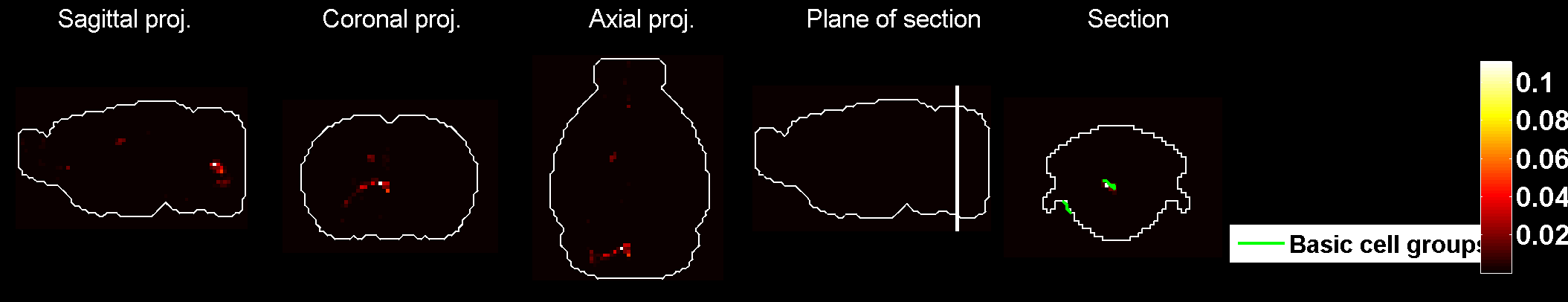
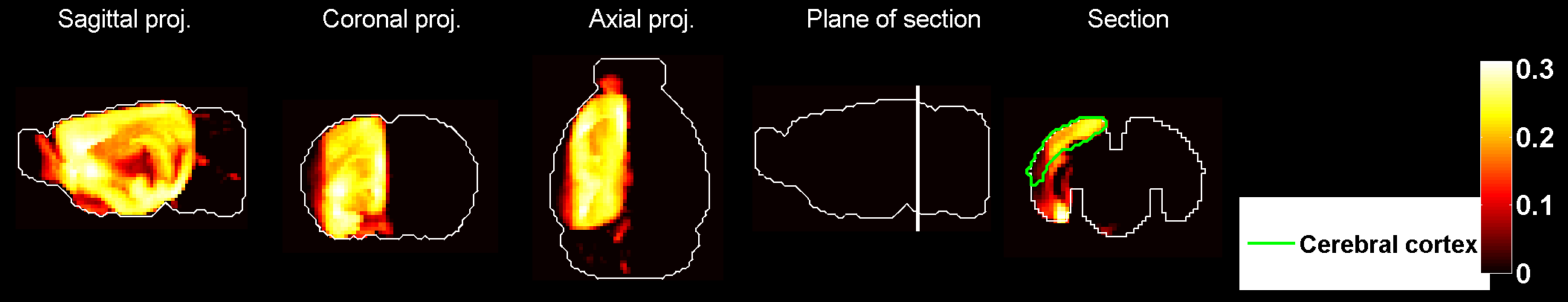
Figure 133: Heat map of the mean density profile for cell type labeled $32$.

Figure 134: Distribution profiles of the density profile of cell type labeled $32$ across random sets of ISH expression energy profiles.

Figure 135: Heat map of the mean correlation profile for cell type labeled $33$.

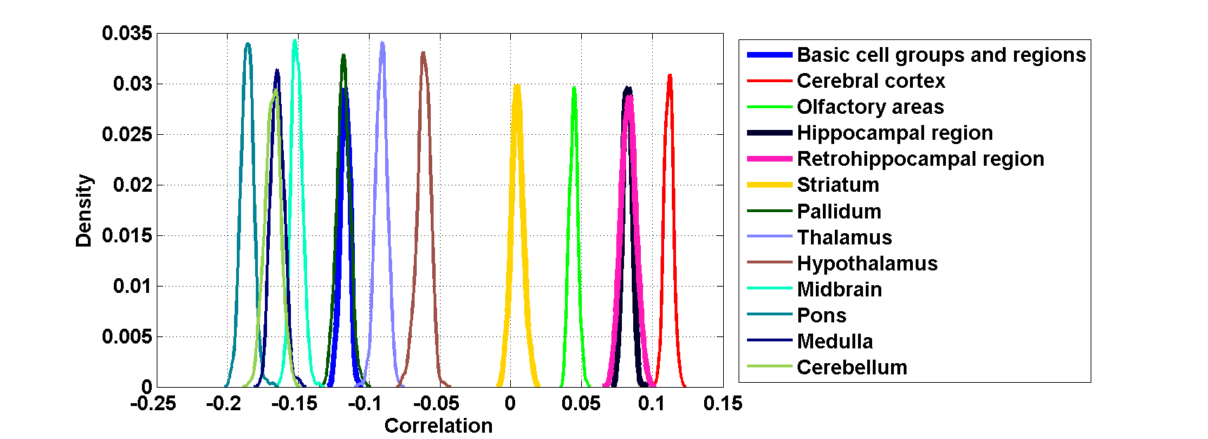
Figure 136: Distribution profiles of the correlations between transcriptome profile of cell type labeled $33$ across random sets of ISH expression energy profiles.

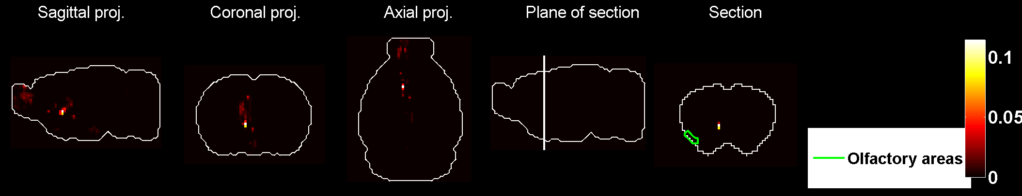
Figure 137: Heat map of the mean density profile for cell type labeled $33$.

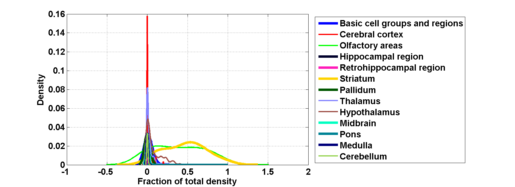
Figure 138: Distribution profiles of the density profile of cell type labeled $33$ across random sets of ISH expression energy profiles.

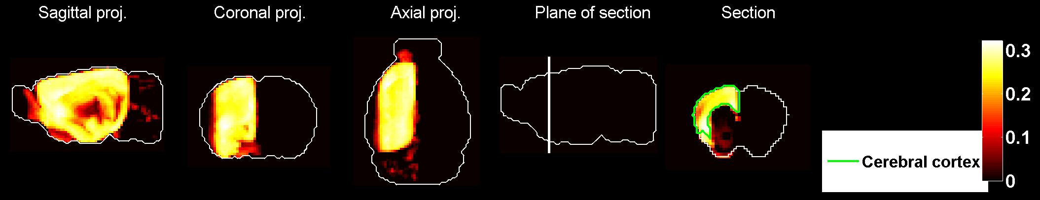
Figure 139: Heat map of the mean correlation profile for cell type labeled $34$.

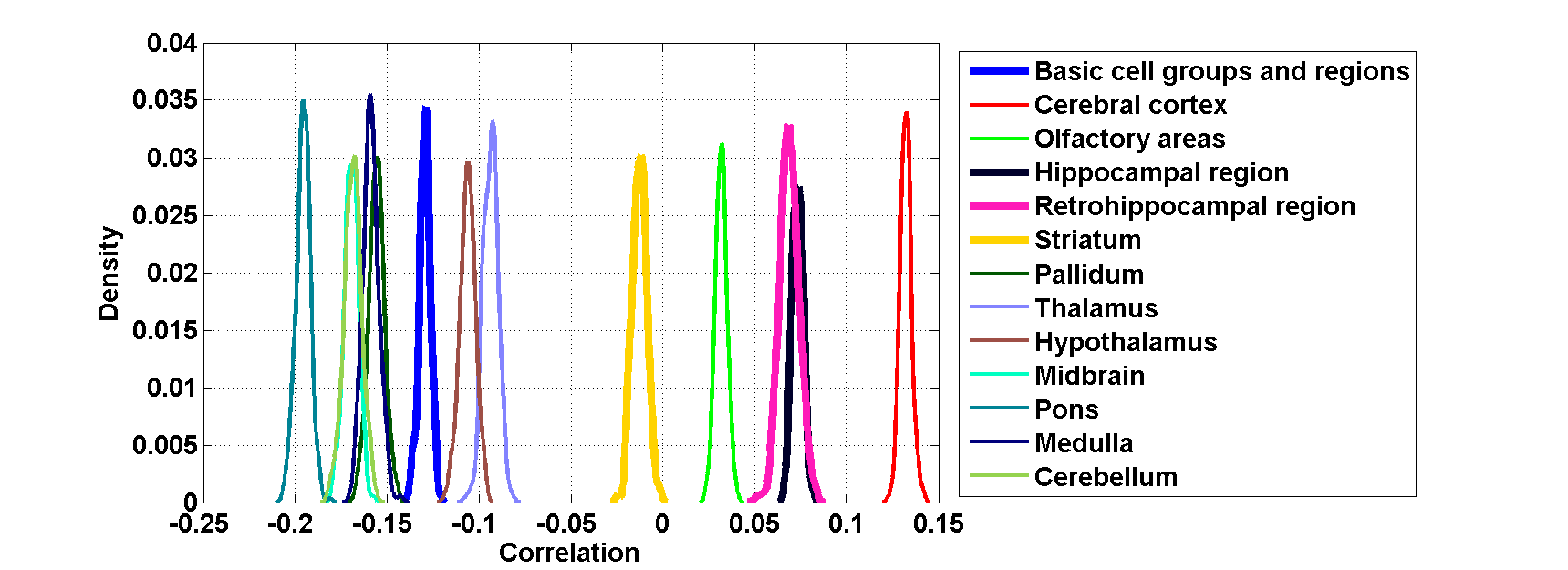
Figure 140: Distribution profiles of the correlations between transcriptome profile of cell type labeled $34$ across random sets of ISH expression energy profiles.

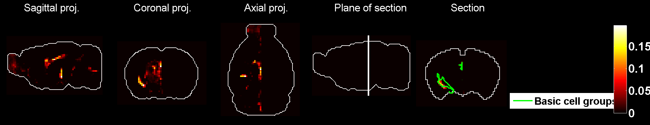
Figure 141: Heat map of the mean density profile for cell type labeled $34$.

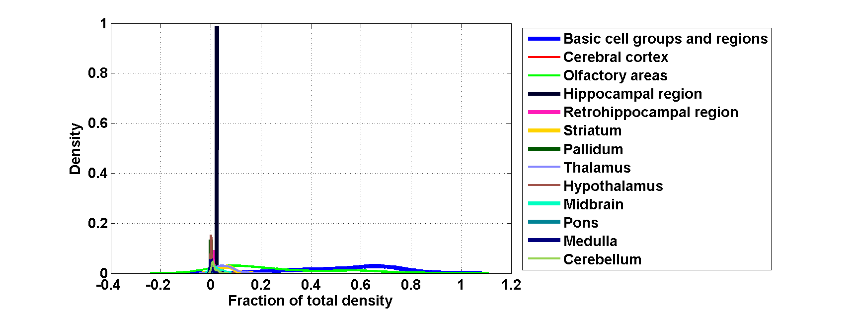
Figure 142: Distribution profiles of the density profile of cell type labeled $34$ across random sets of ISH expression energy profiles.

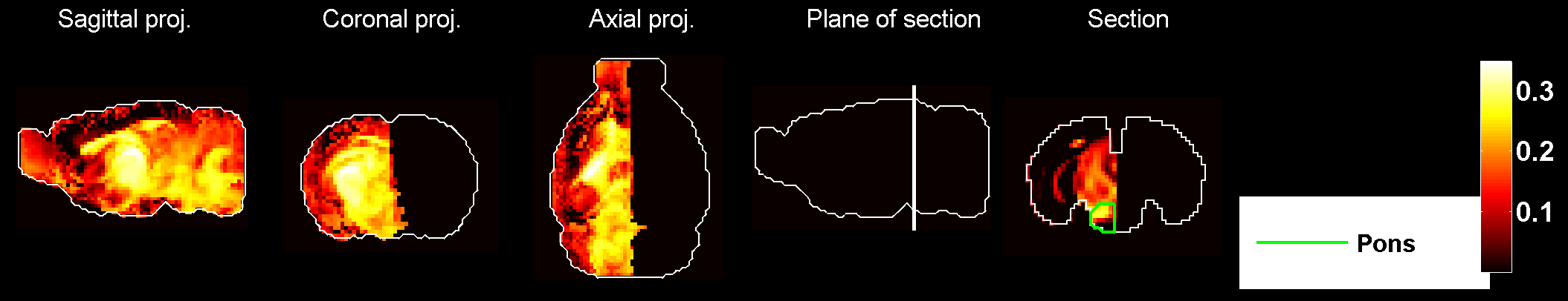
Figure 143: Heat map of the mean correlation profile for cell type labeled $35$.

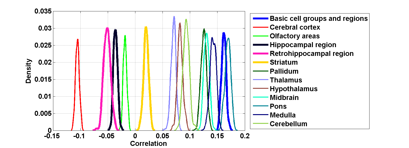
Figure 144: Distribution profiles of the correlations between transcriptome profile of cell type labeled $35$ across random sets of ISH expression energy profiles.

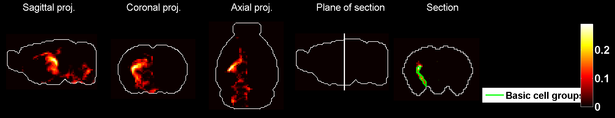
Figure 145: Heat map of the mean density profile for cell type labeled $35$.

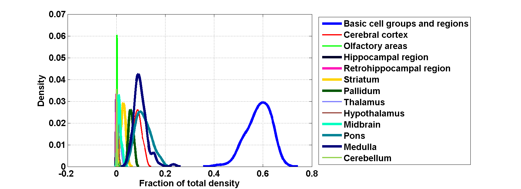
Figure 146: Distribution profiles of the density profile of cell type labeled $35$ across random sets of ISH expression energy profiles.

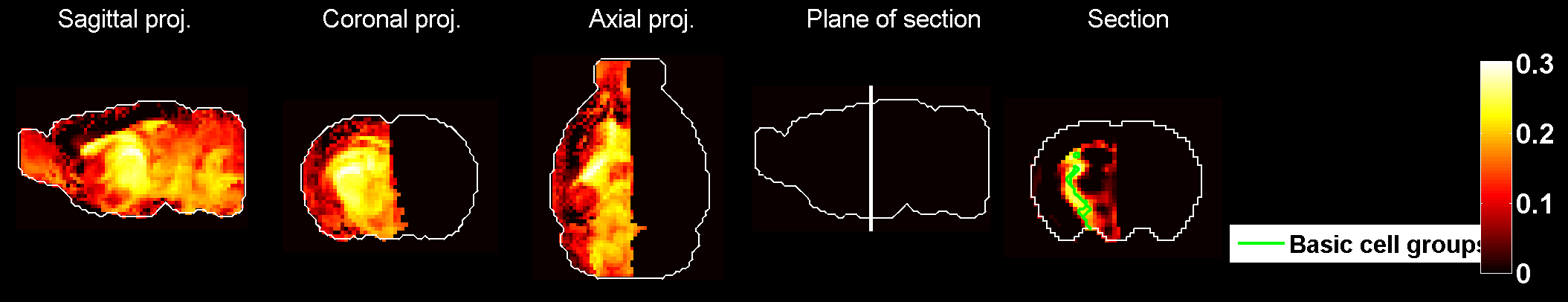
Figure 147: Heat map of the mean correlation profile for cell type labeled $36$.

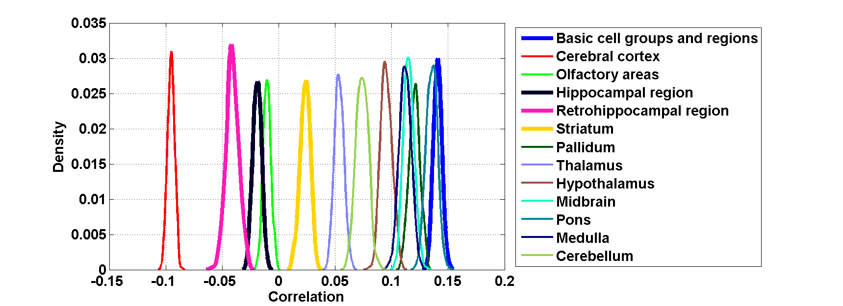
Figure 148: Distribution profiles of the correlations between transcriptome profile of cell type labeled $36$ across random sets of ISH expression energy profiles.

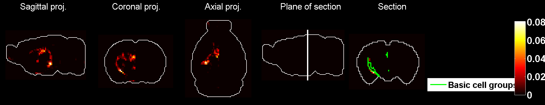
Figure 149: Heat map of the mean density profile for cell type labeled $36$.

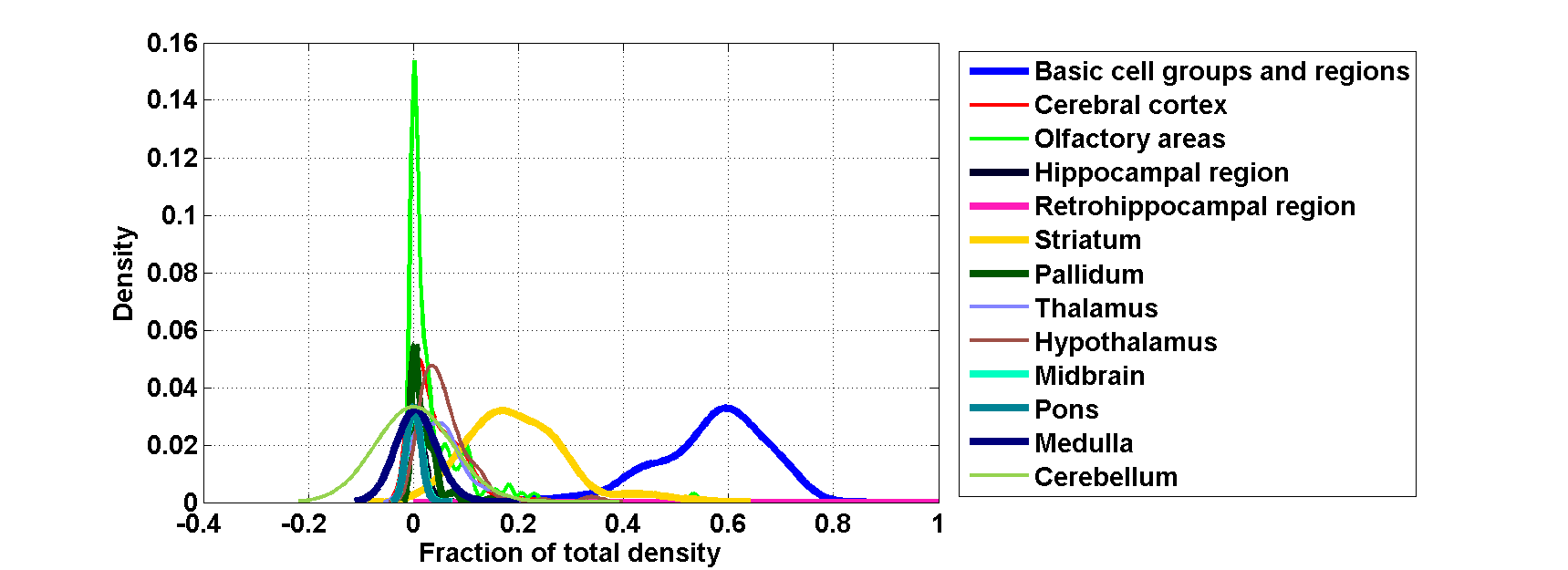
Figure 150: Distribution profiles of the density profile of cell type labeled $36$ across random sets of ISH expression energy profiles.

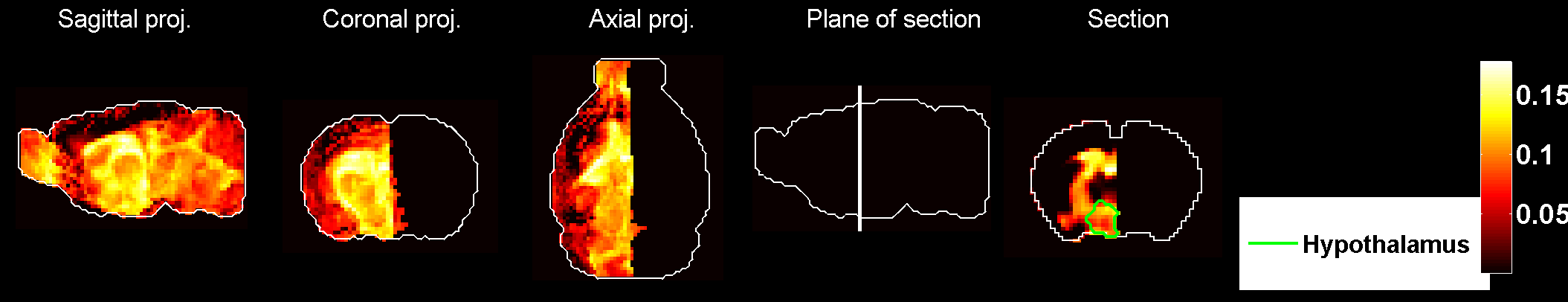
Figure 151: Heat map of the mean correlation profile for cell type labeled $37$.

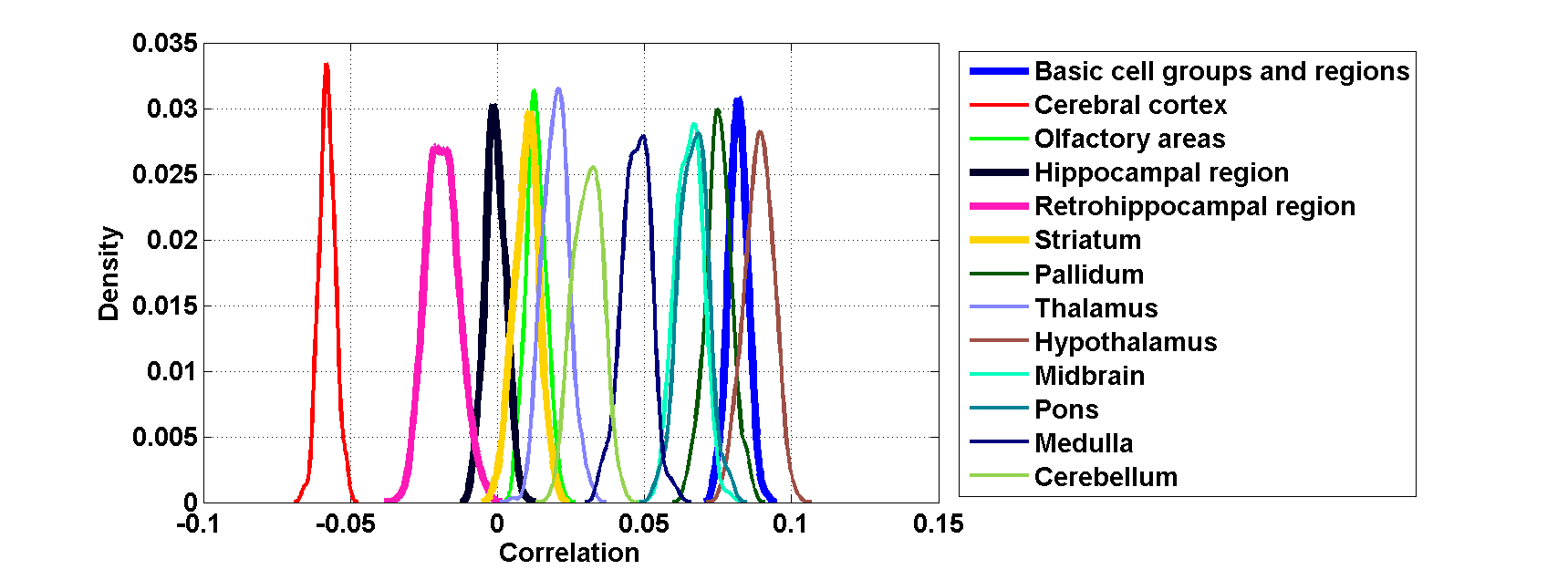
Figure 152: Distribution profiles of the correlations between transcriptome profile of cell type labeled $37$ across random sets of ISH expression energy profiles.

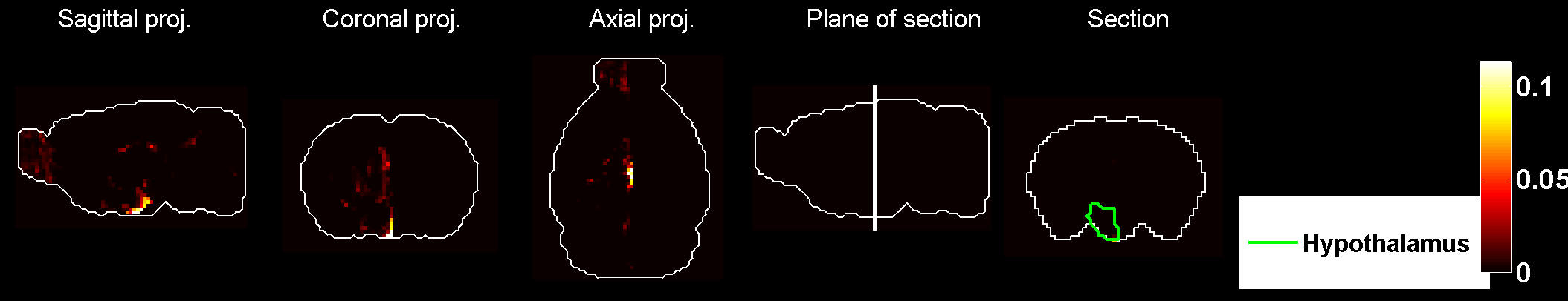
Figure 153: Heat map of the mean density profile for cell type labeled $37$.

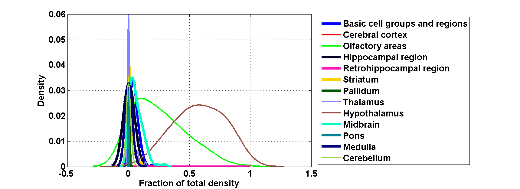
Figure 154: Distribution profiles of the density profile of cell type labeled $37$ across random sets of ISH expression energy profiles.

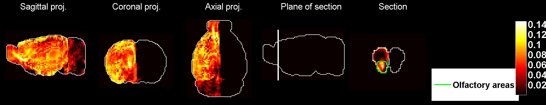
Figure 155: Heat map of the mean correlation profile for cell type labeled $38$.

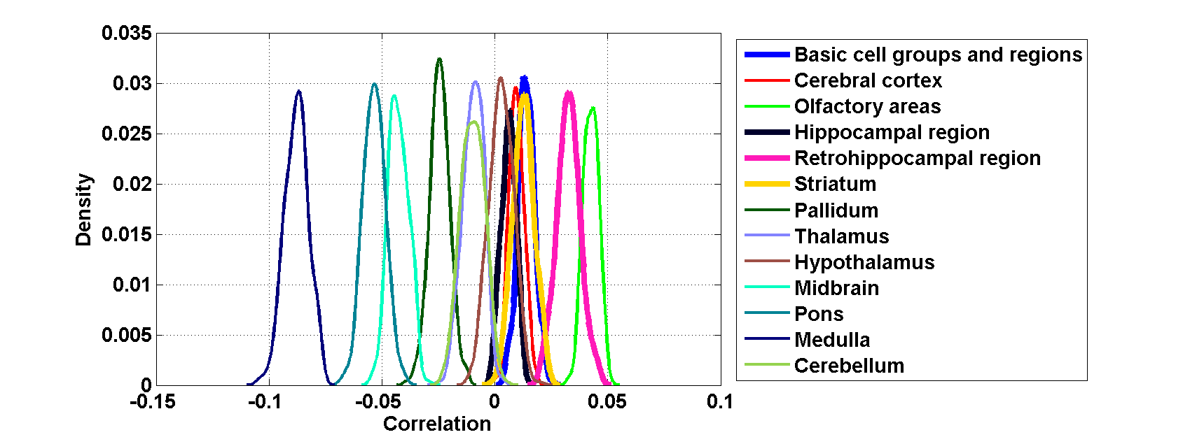
Figure 156: Distribution profiles of the correlations between transcriptome profile of cell type labeled $38$ across random sets of ISH expression energy profiles.

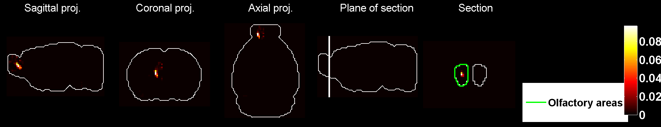
Figure 157: Heat map of the mean density profile for cell type labeled $38$.

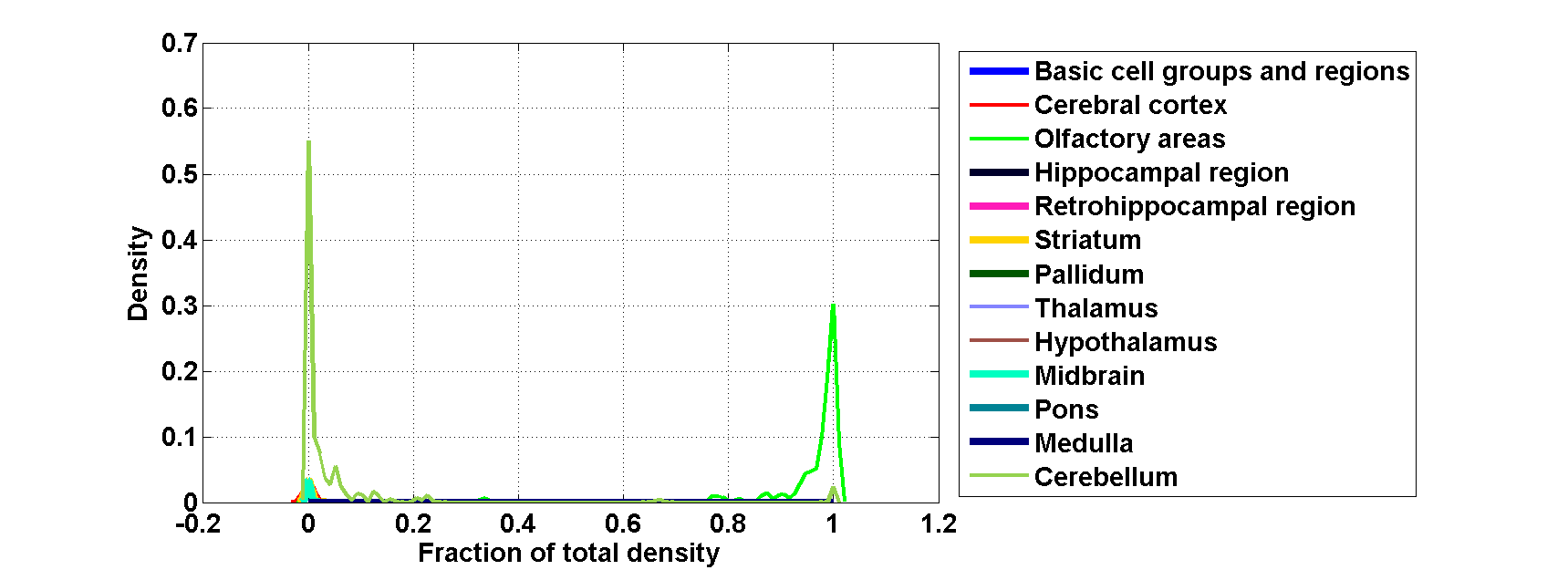
Figure 158: Distribution profiles of the density profile of cell type labeled $38$ across random sets of ISH expression energy profiles.

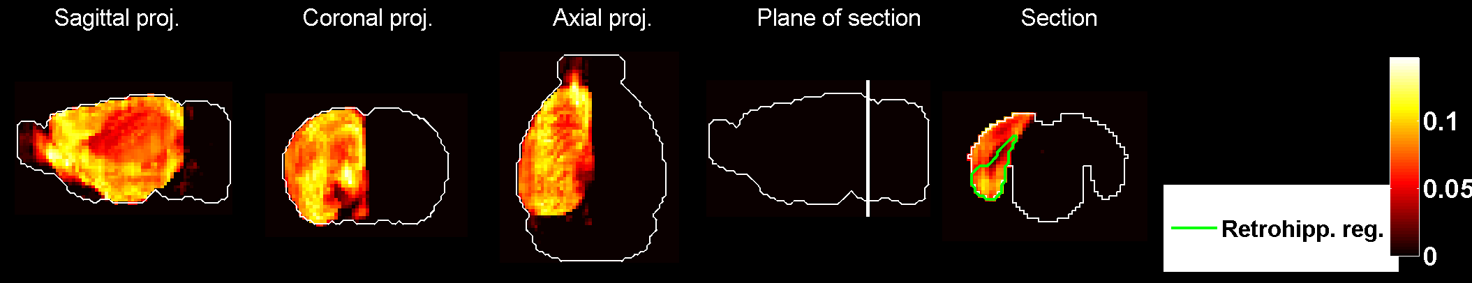
Figure 159: Heat map of the mean correlation profile for cell type labeled $39$.

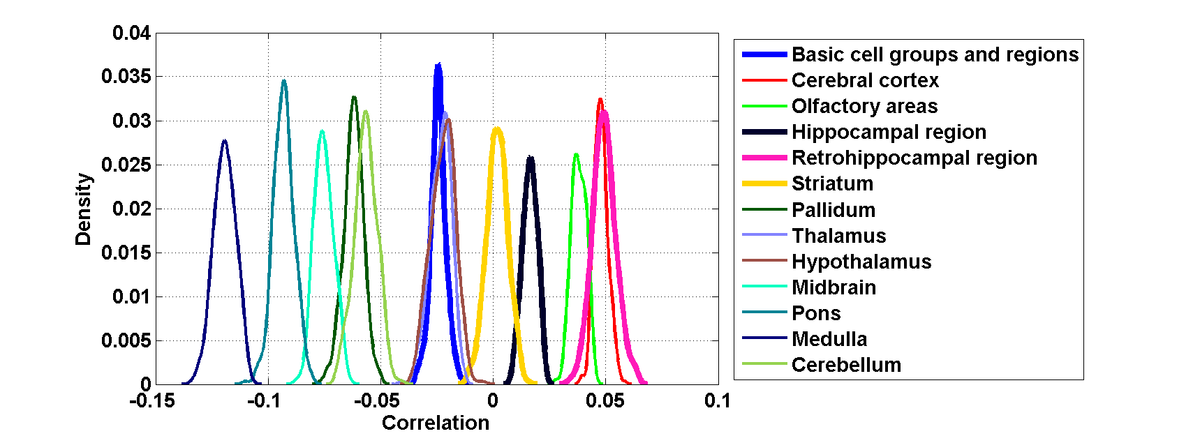
Figure 160: Distribution profiles of the correlations between transcriptome profile of cell type labeled $39$ across random sets of ISH expression energy profiles.

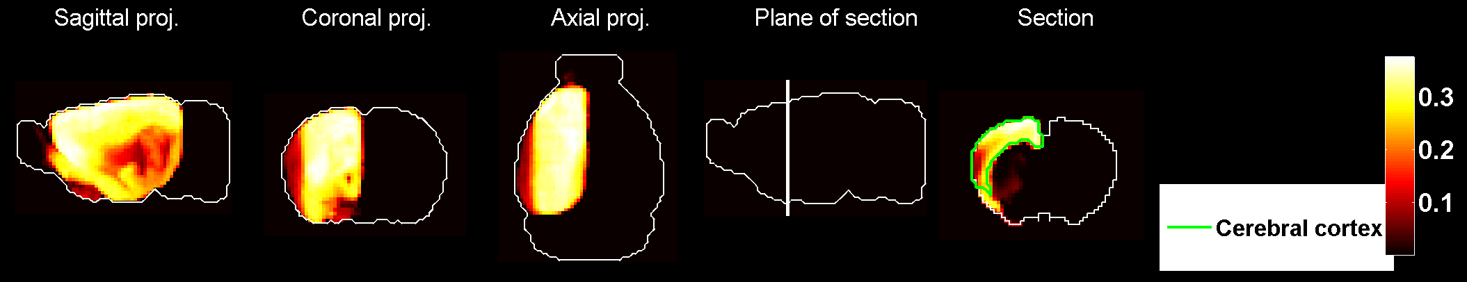
Figure 161: Heat map of the mean density profile for cell type labeled $39$.

Figure 162: Distribution profiles of the density profile of cell type labeled $39$ across random sets of ISH expression energy profiles.

Figure 163: Heat map of the mean correlation profile for cell type labeled $40$.

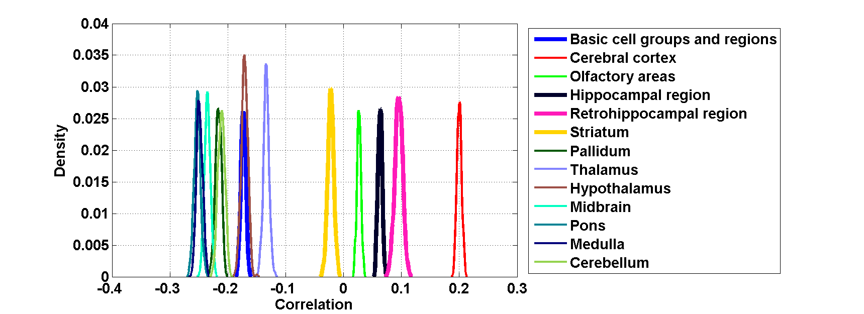
Figure 164: Distribution profiles of the correlations between transcriptome profile of cell type labeled $40$ across random sets of ISH expression energy profiles.

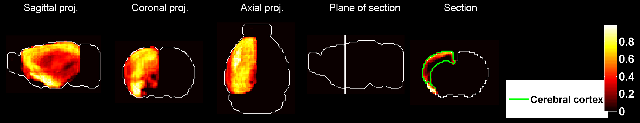
Figure 165: Heat map of the mean density profile for cell type labeled $40$.

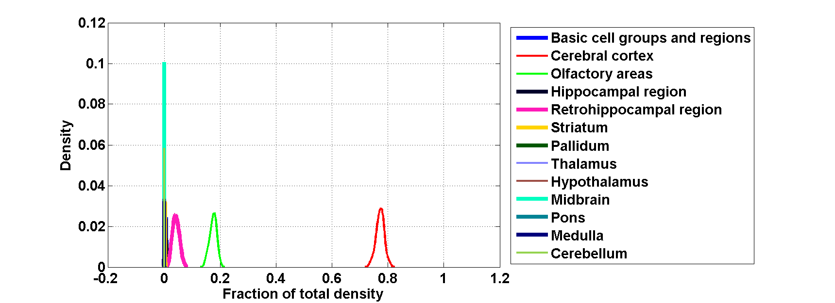
Figure 166: Distribution profiles of the density profile of cell type labeled $40$ across random sets of ISH expression energy profiles.

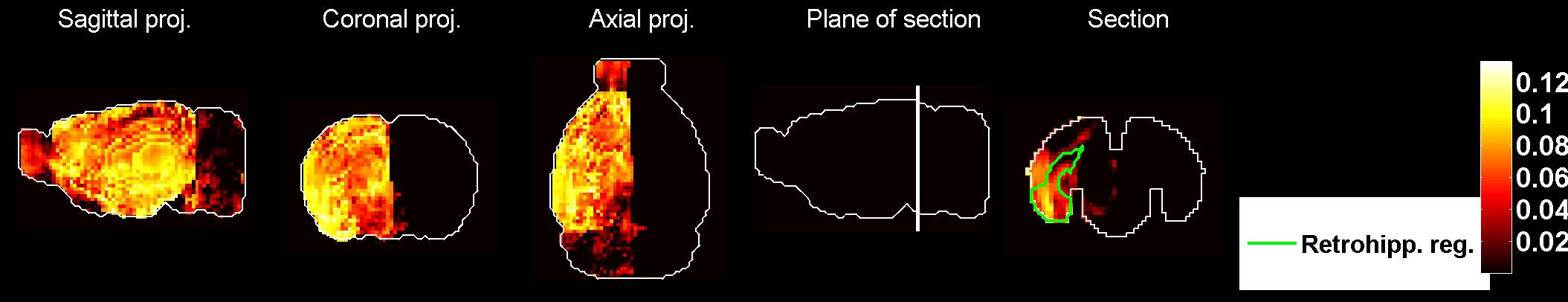
Figure 167: Heat map of the mean correlation profile for cell type labeled $41$.

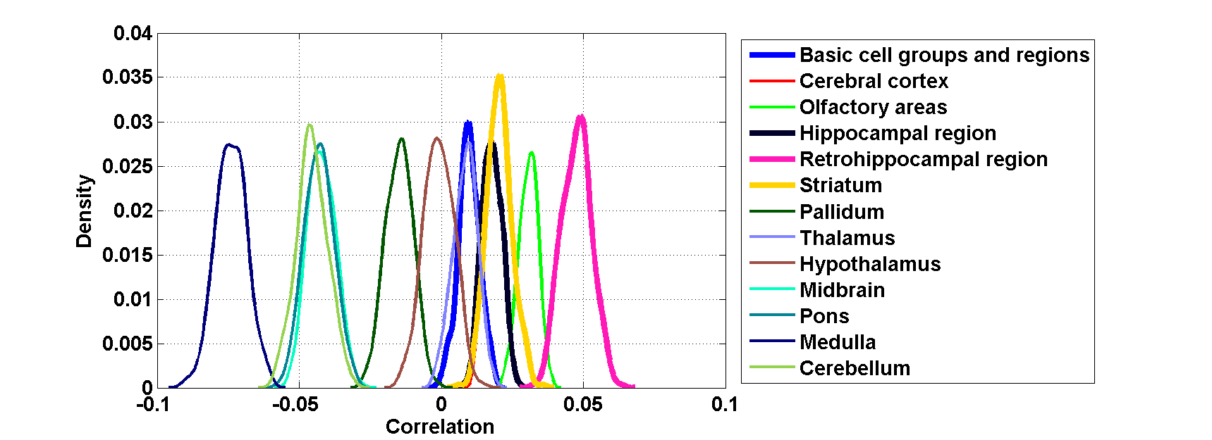
Figure 168: Distribution profiles of the correlations between transcriptome profile of cell type labeled $41$ across random sets of ISH expression energy profiles.

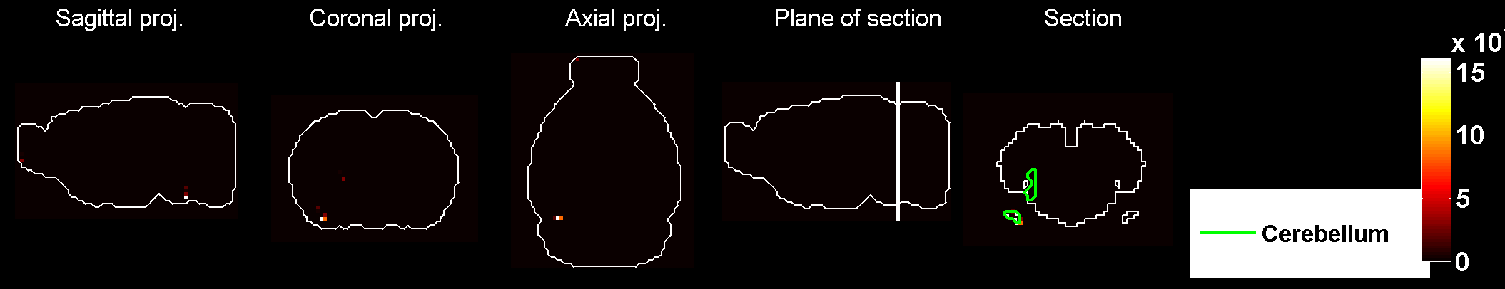
Figure 169: Heat map of the mean density profile for cell type labeled $41$.

Figure 170: Distribution profiles of the density profile of cell type labeled $41$ across random sets of ISH expression energy profiles.

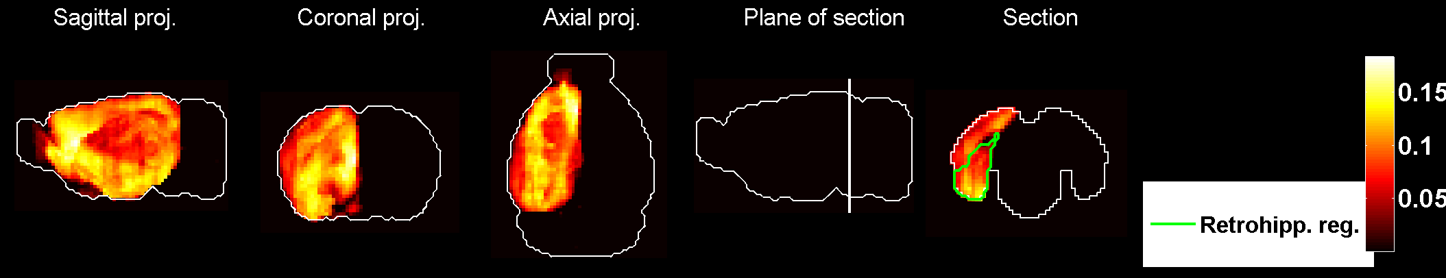
Figure 171: Heat map of the mean correlation profile for cell type labeled $42$.

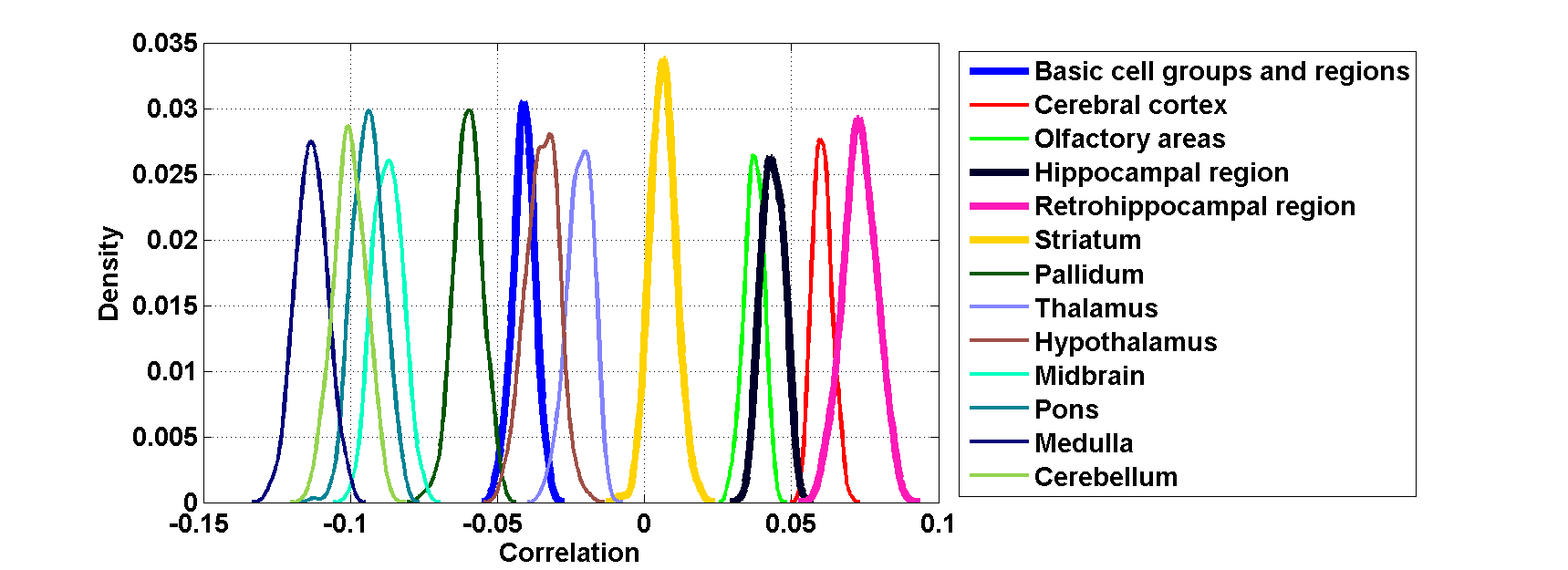
Figure 172: Distribution profiles of the correlations between transcriptome profile of cell type labeled $42$ across random sets of ISH expression energy profiles.

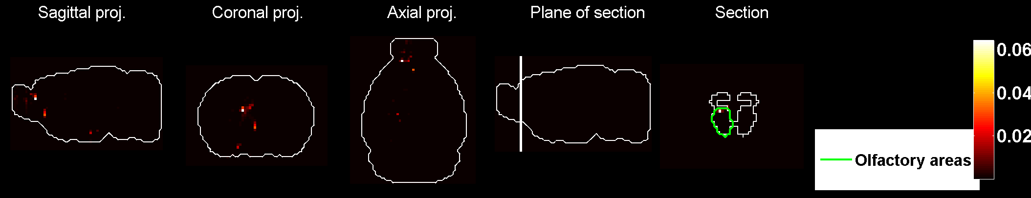
Figure 173: Heat map of the mean density profile for cell type labeled $42$.

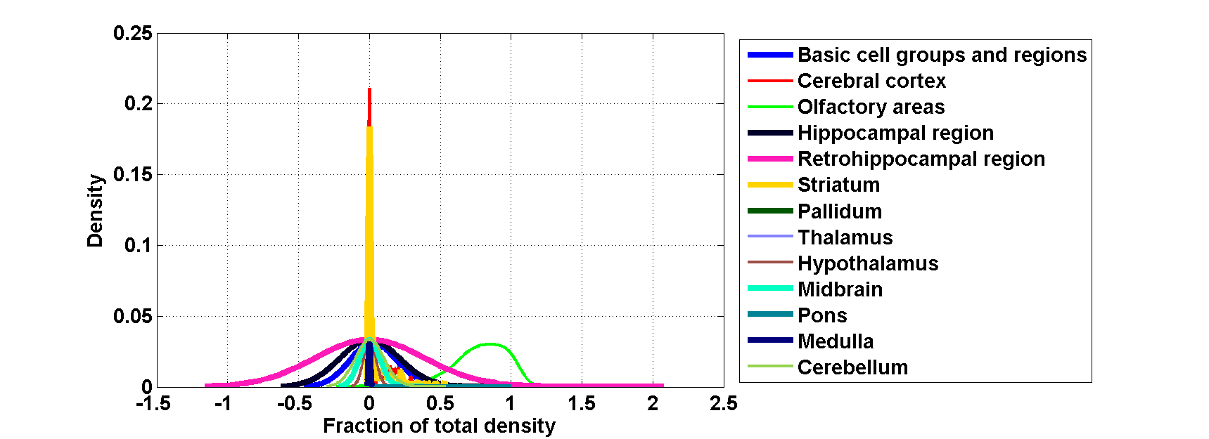
Figure 174: Distribution profiles of the density profile of cell type labeled $42$ across random sets of ISH expression energy profiles.

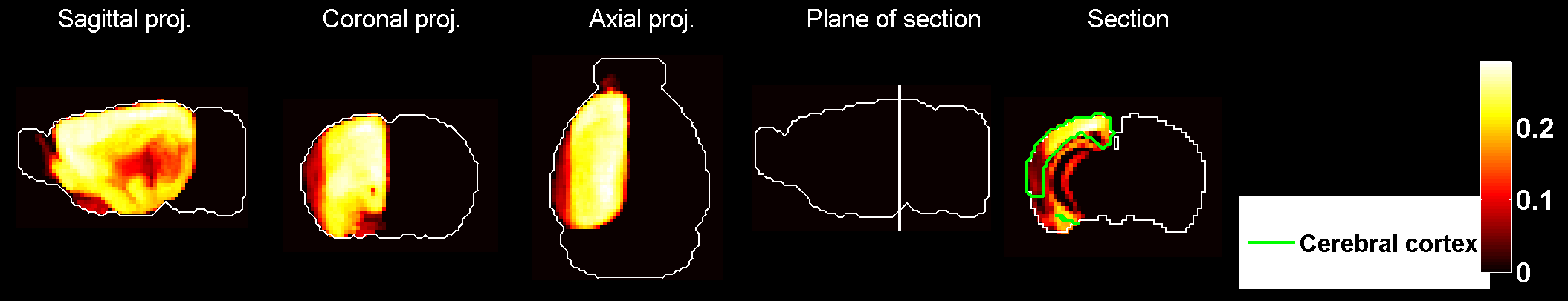
Figure 175: Heat map of the mean correlation profile for cell type labeled $43$.

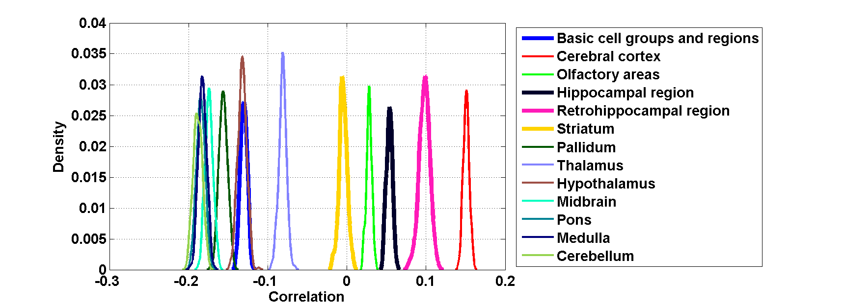
Figure 176: Distribution profiles of the correlations between transcriptome profile of cell type labeled $43$ across random sets of ISH expression energy profiles.

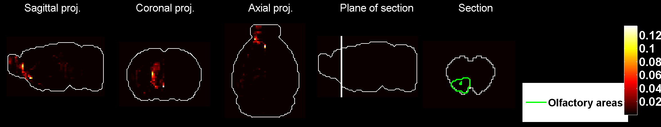
Figure 177: Heat map of the mean density profile for cell type labeled $43$.

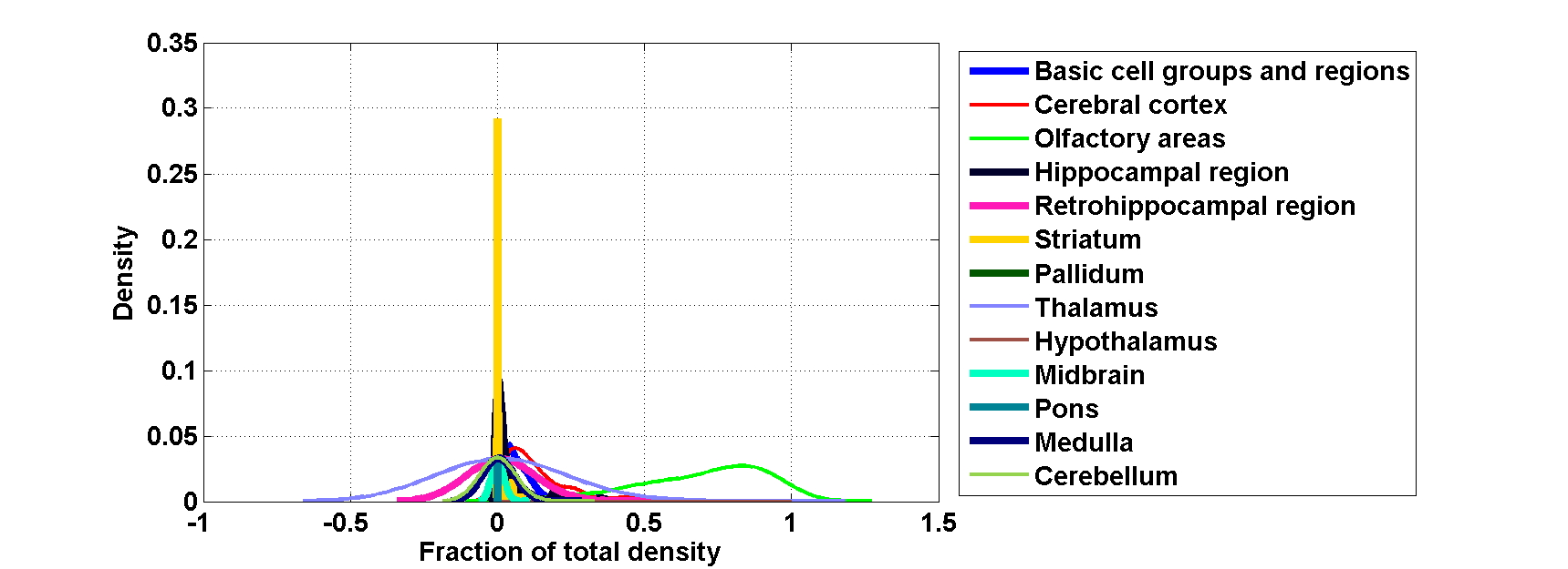
Figure 178: Distribution profiles of the density profile of cell type labeled $43$ across random sets of ISH expression energy profiles.

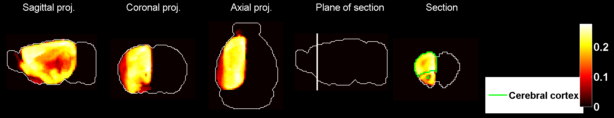
Figure 179: Heat map of the mean correlation profile for cell type labeled $44$.

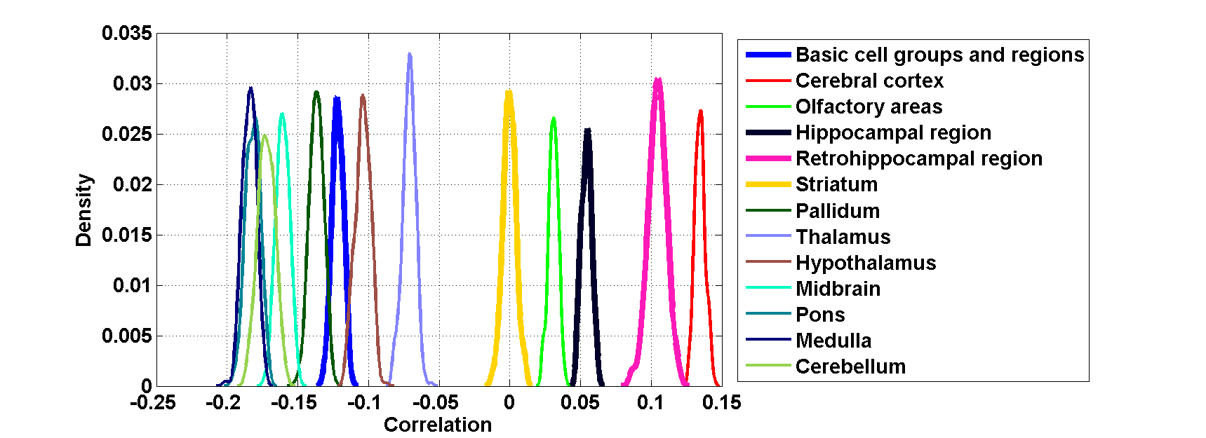
Figure 180: Distribution profiles of the correlations between transcriptome profile of cell type labeled $44$ across random sets of ISH expression energy profiles.

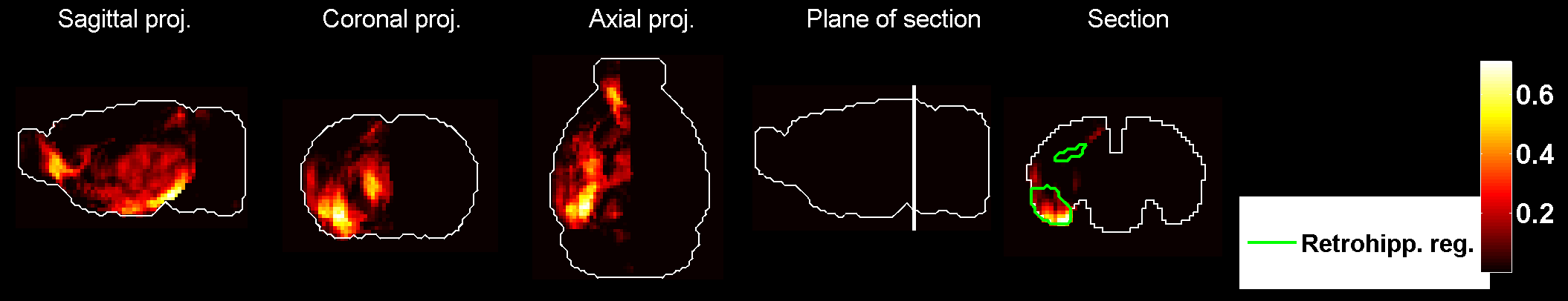
Figure 181: Heat map of the mean density profile for cell type labeled $44$.

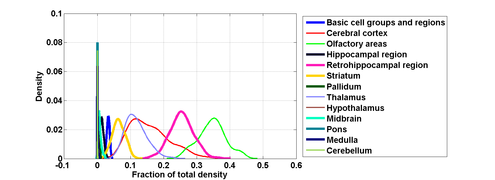
Figure 182: Distribution profiles of the density profile of cell type labeled $44$ across random sets of ISH expression energy profiles.

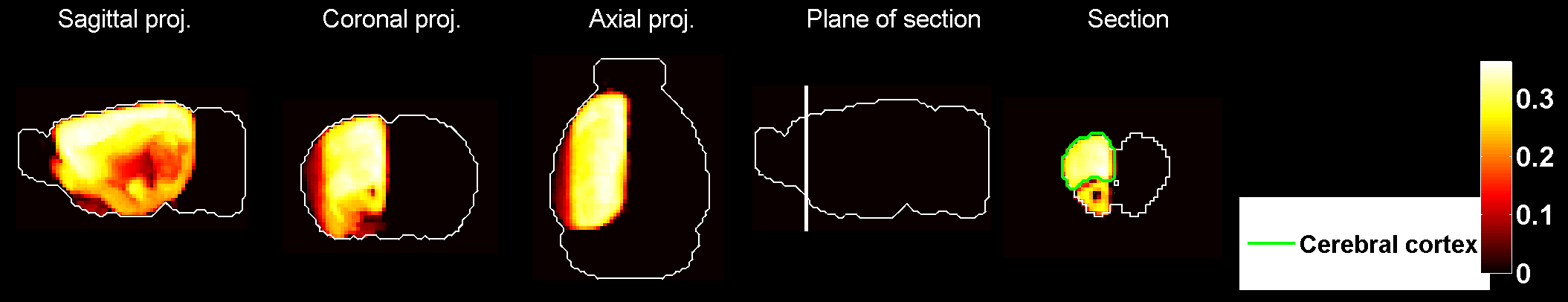
Figure 183: Heat map of the mean correlation profile for cell type labeled $45$.

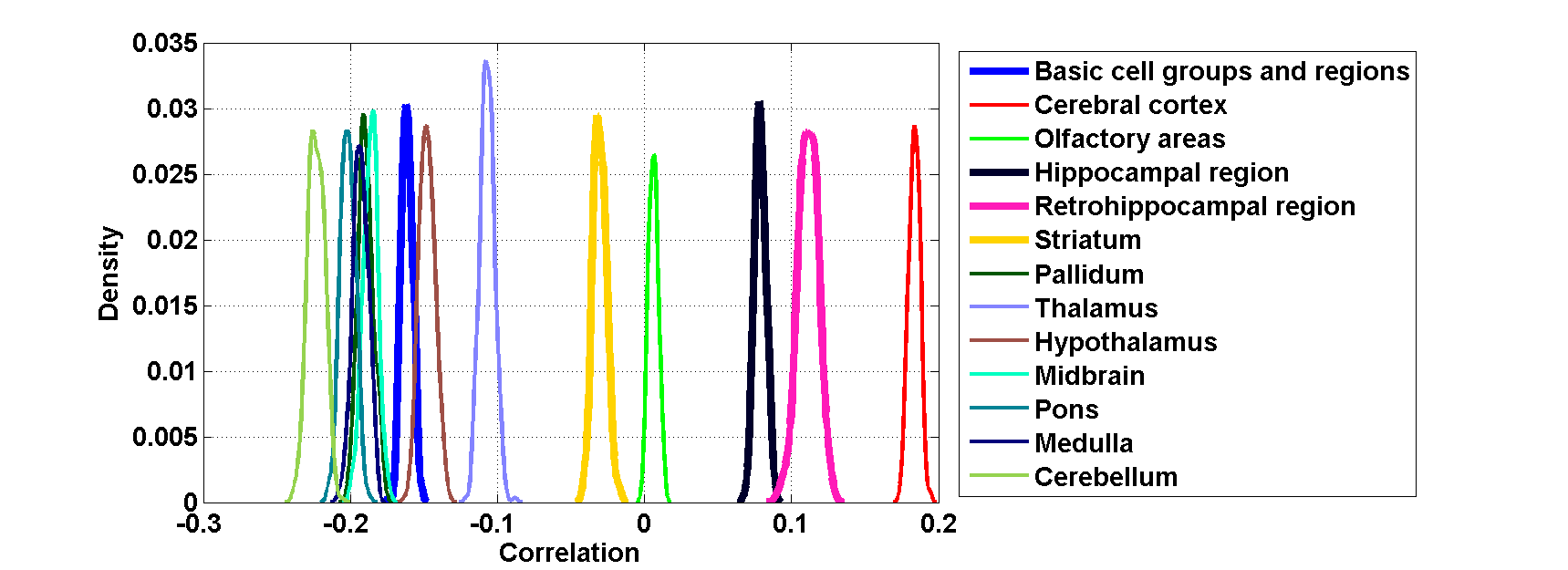
Figure 184: Distribution profiles of the correlations between transcriptome profile of cell type labeled $45$ across random sets of ISH expression energy profiles.

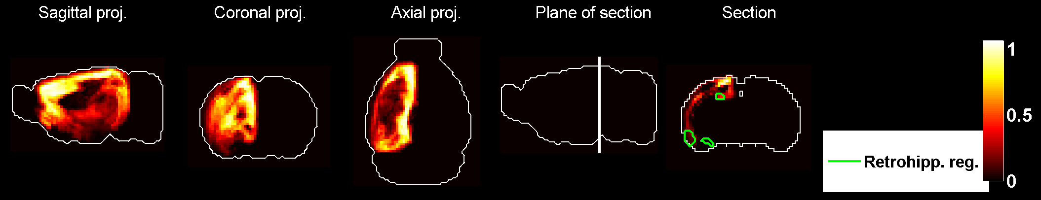
Figure 185: Heat map of the mean density profile for cell type labeled $45$.

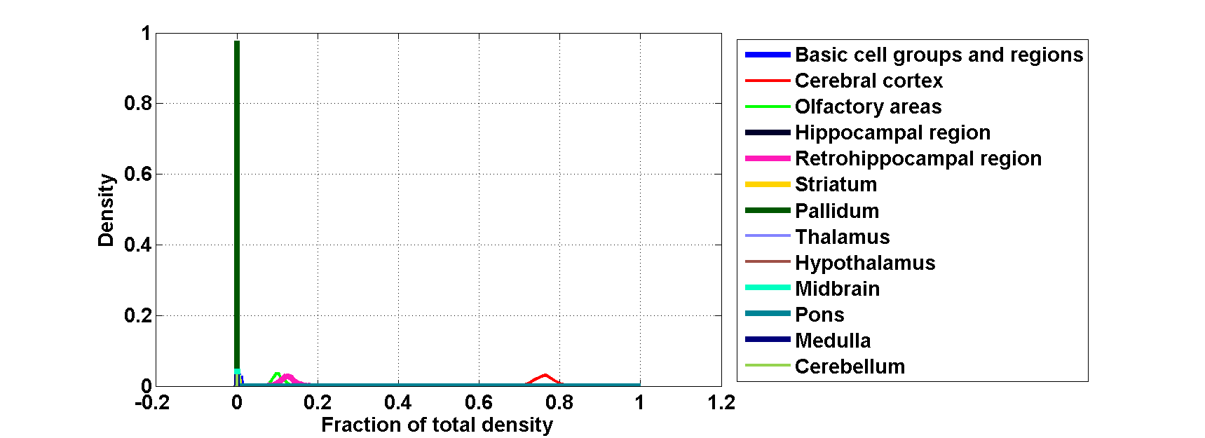
Figure 186: Distribution profiles of the density profile of cell type labeled $45$ across random sets of ISH expression energy profiles.

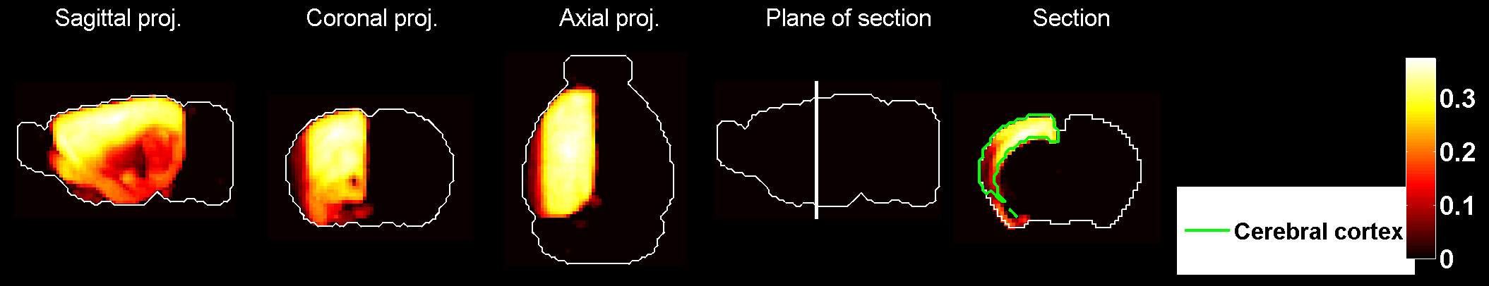
Figure 187: Heat map of the mean correlation profile for cell type labeled $46$.

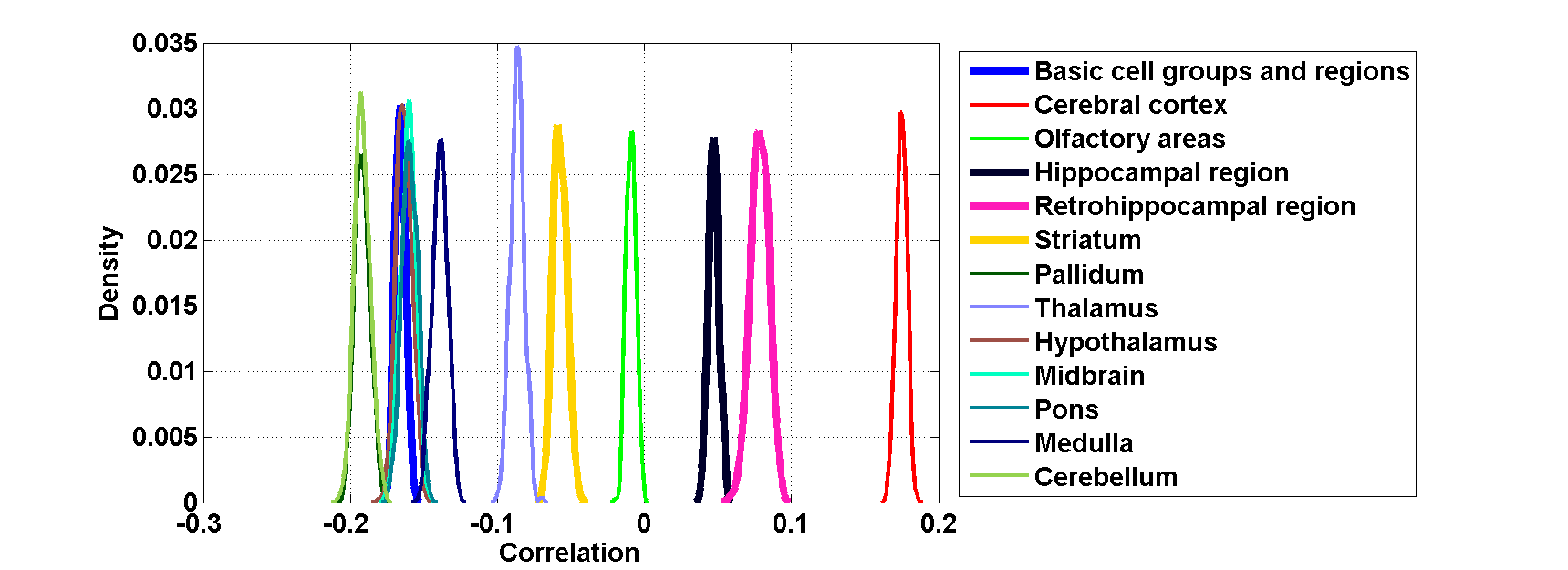
Figure 188: Distribution profiles of the correlations between transcriptome profile of cell type labeled $46$ across random sets of ISH expression energy profiles.

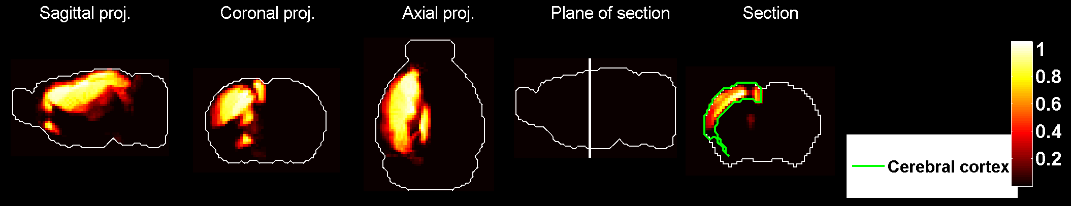
Figure 189: Heat map of the mean density profile for cell type labeled $46$.

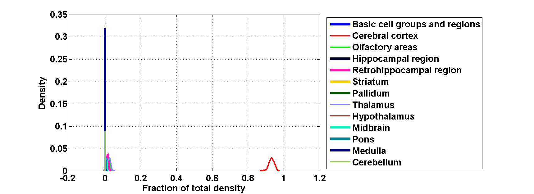
Figure 190: Distribution profiles of the density profile of cell type labeled $46$ across random sets of ISH expression energy profiles.

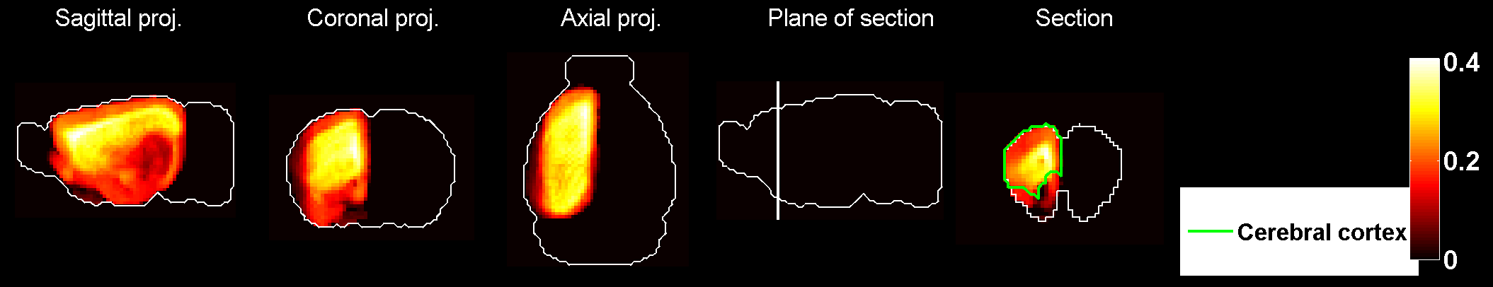
Figure 191: Heat map of the mean correlation profile for cell type labeled $47$.

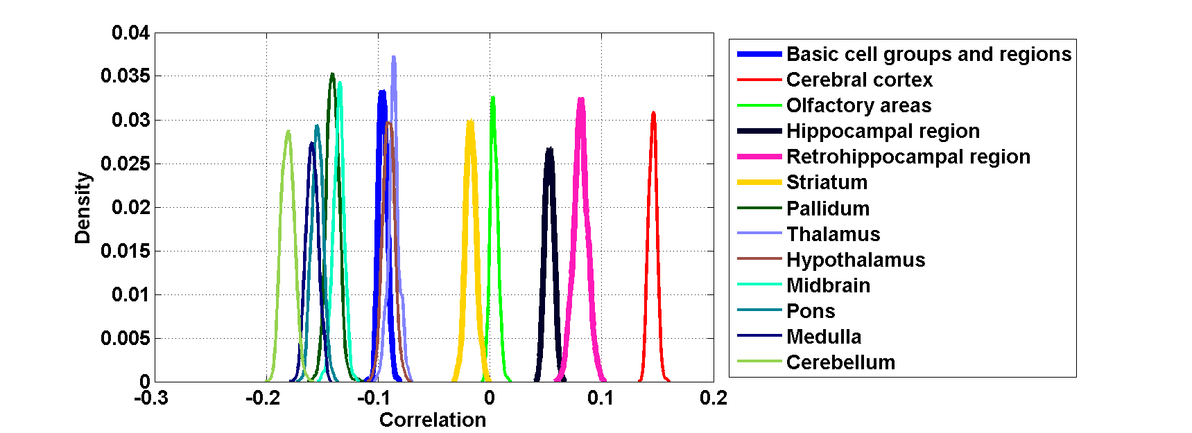
Figure 192: Distribution profiles of the correlations between transcriptome profile of cell type labeled $47$ across random sets of ISH expression energy profiles.

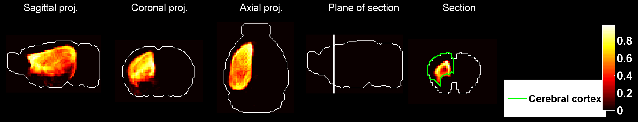
Figure 193: Heat map of the mean density profile for cell type labeled $47$.

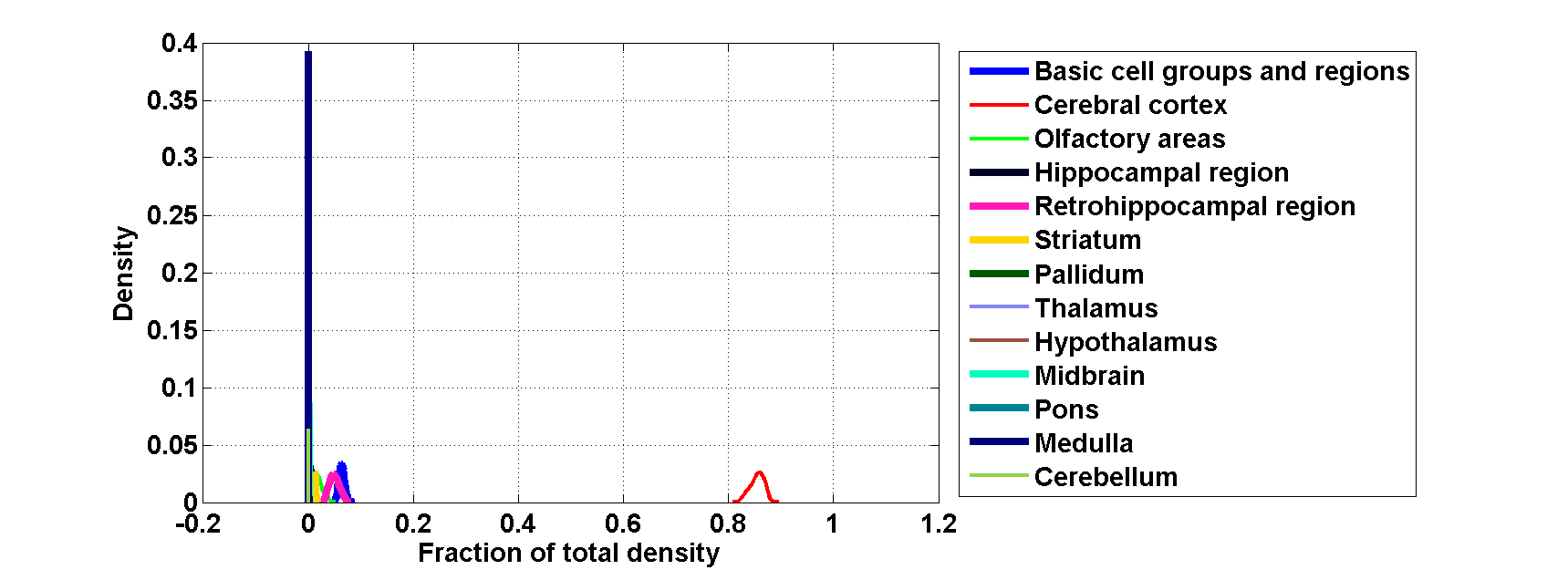
Figure 194: Distribution profiles of the density profile of cell type labeled $47$ across random sets of ISH expression energy profiles.

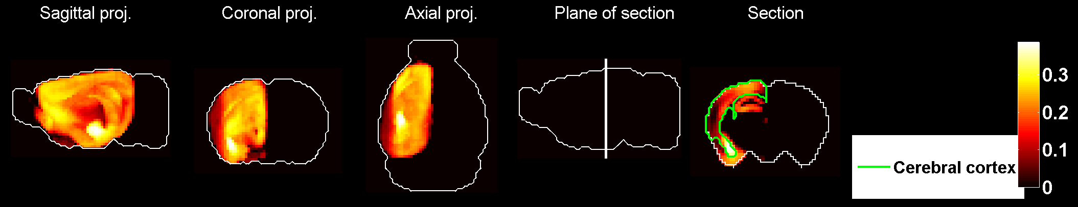
Figure 195: Heat map of the mean correlation profile for cell type labeled $48$.

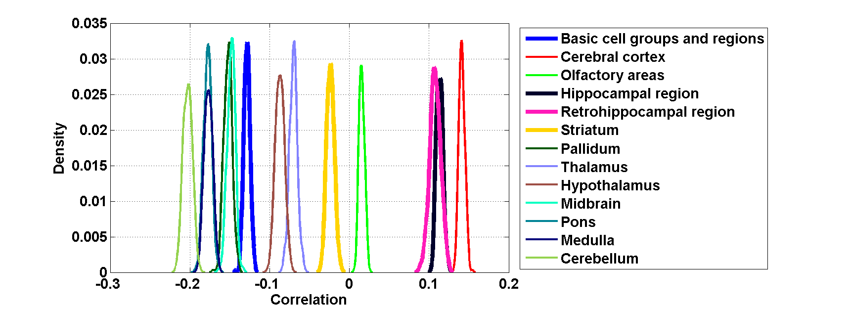
Figure 196: Distribution profiles of the correlations between transcriptome profile of cell type labeled $48$ across random sets of ISH expression energy profiles.

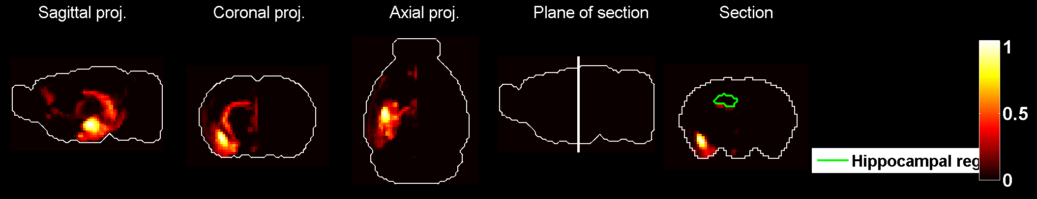
Figure 197: Heat map of the mean density profile for cell type labeled $48$.

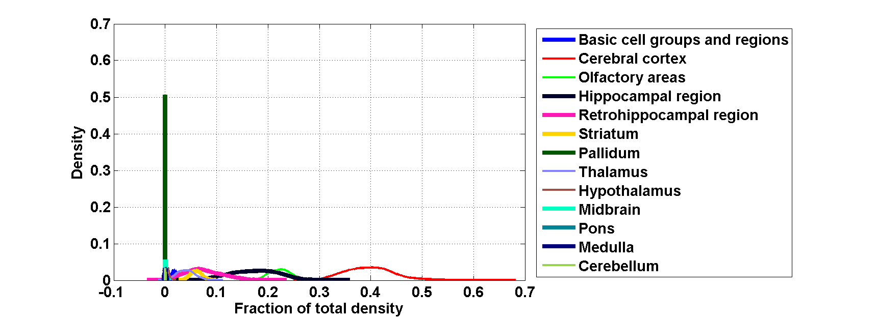
Figure 198: Distribution profiles of the density profile of cell type labeled $48$ across random sets of ISH expression energy profiles.

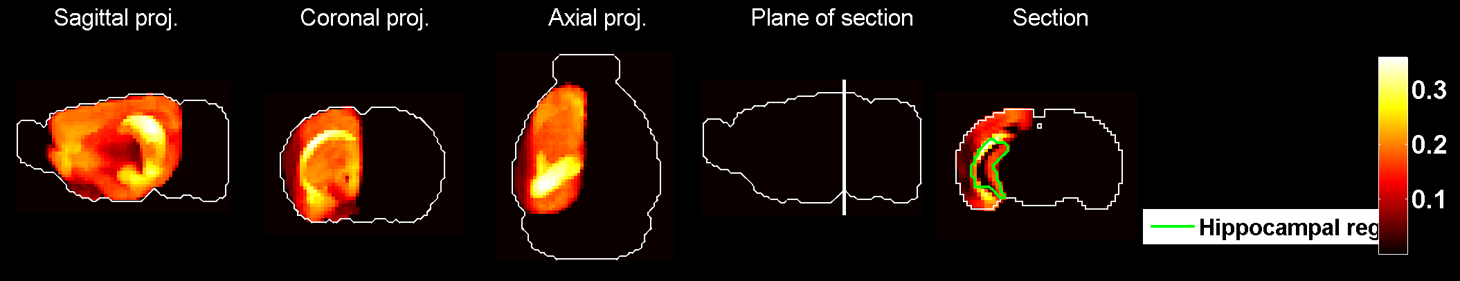
Figure 199: Heat map of the mean correlation profile for cell type labeled $49$.

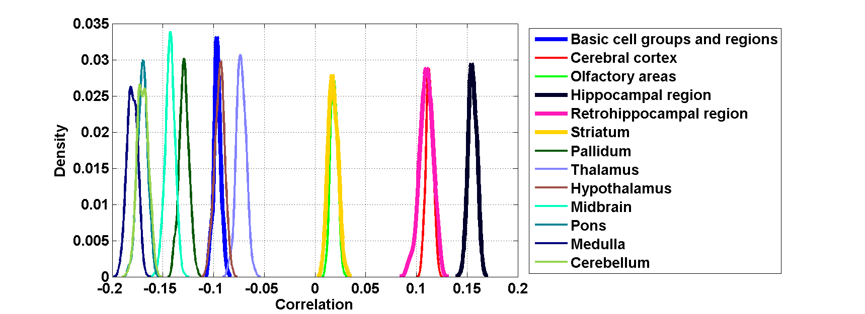
Figure 200: Distribution profiles of the correlations between transcriptome profile of cell type labeled $49$ across random sets of ISH expression energy profiles.

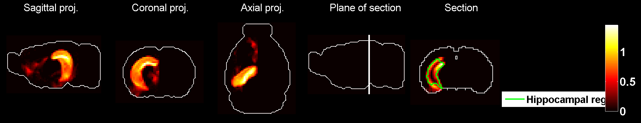
Figure 201: Heat map of the mean density profile for cell type labeled $49$.

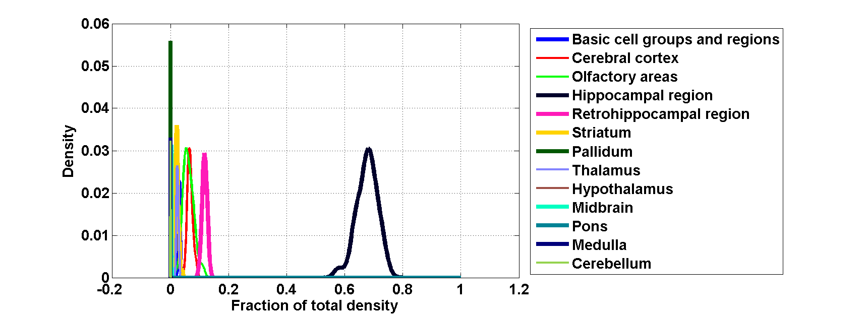
Figure 202: Distribution profiles of the density profile of cell type labeled $49$ across random sets of ISH expression energy profiles.

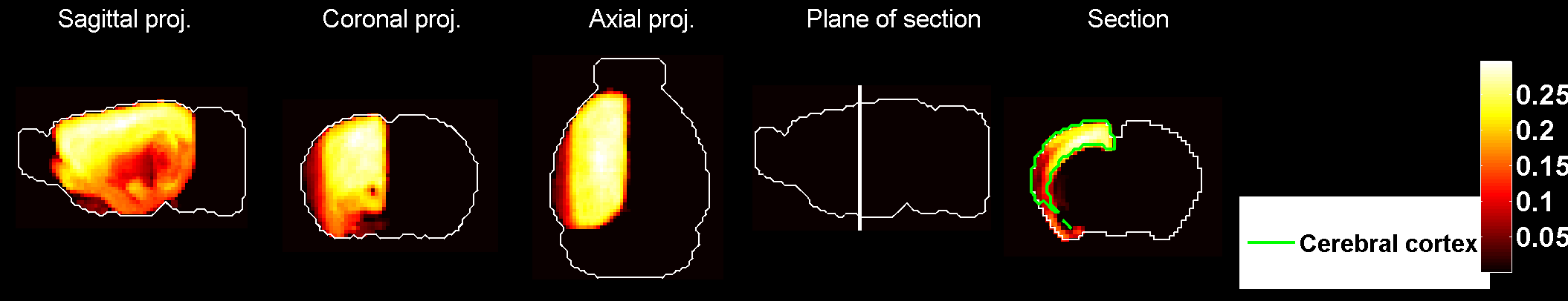
Figure 203: Heat map of the mean correlation profile for cell type labeled $50$.

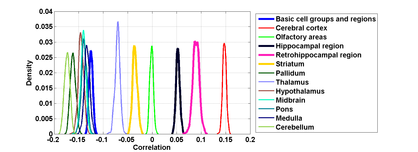
Figure 204: Distribution profiles of the correlations between transcriptome profile of cell type labeled $50$ across random sets of ISH expression energy profiles.

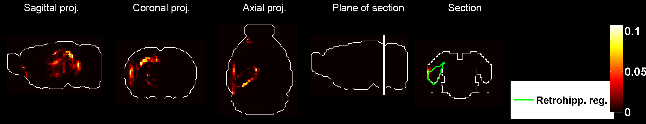
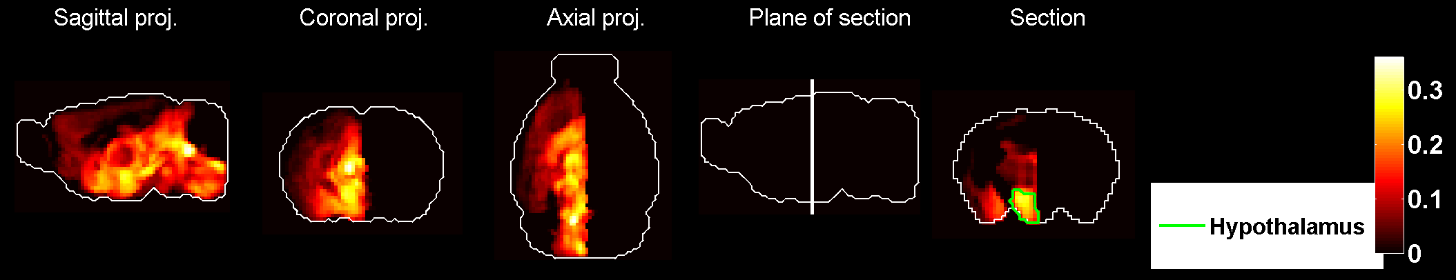
Figure 205: Heat map of the mean density profile for cell type labeled $50$.

Figure 206: Distribution profiles of the density profile of cell type labeled $50$ across random sets of ISH expression energy profiles.

Figure 207: Heat map of the mean correlation profile for cell type labeled $51$.

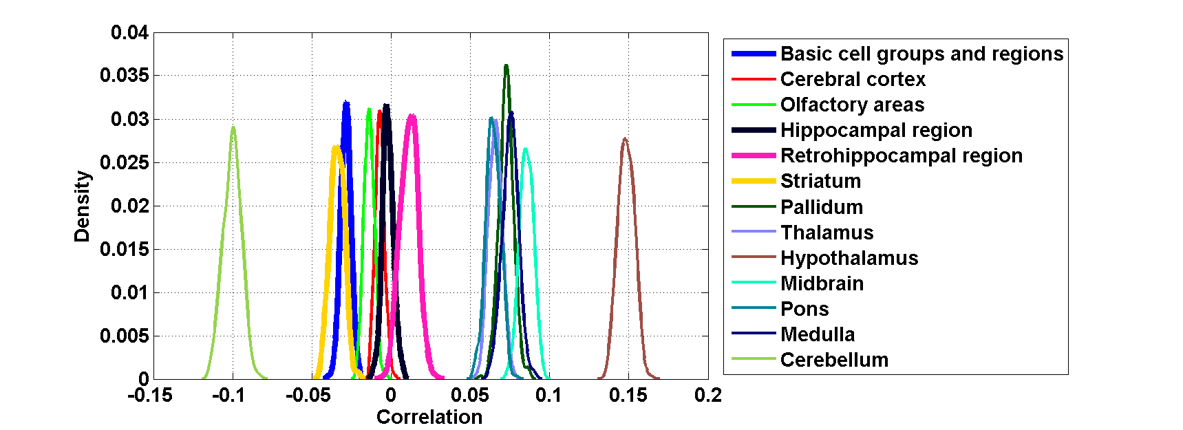
Figure 208: Distribution profiles of the correlations between transcriptome profile of cell type labeled $51$ across random sets of ISH expression energy profiles.

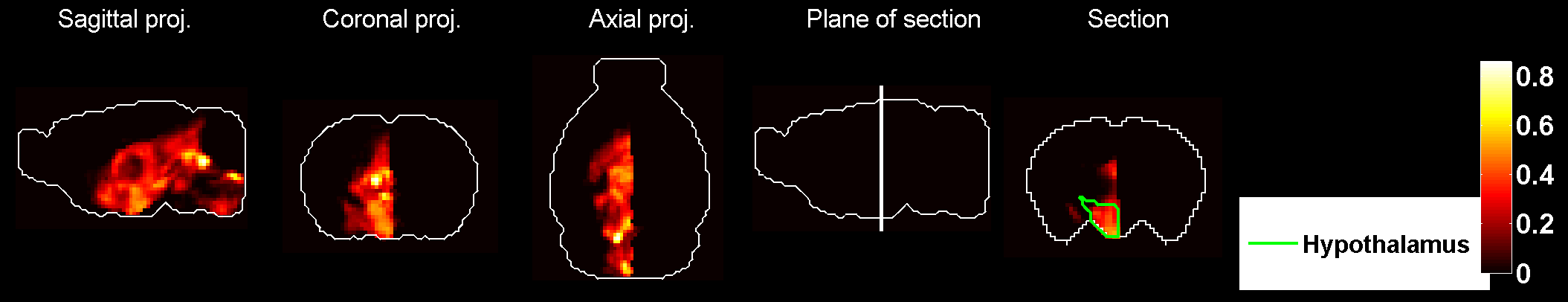
Figure 209: Heat map of the mean density profile for cell type labeled $51$.

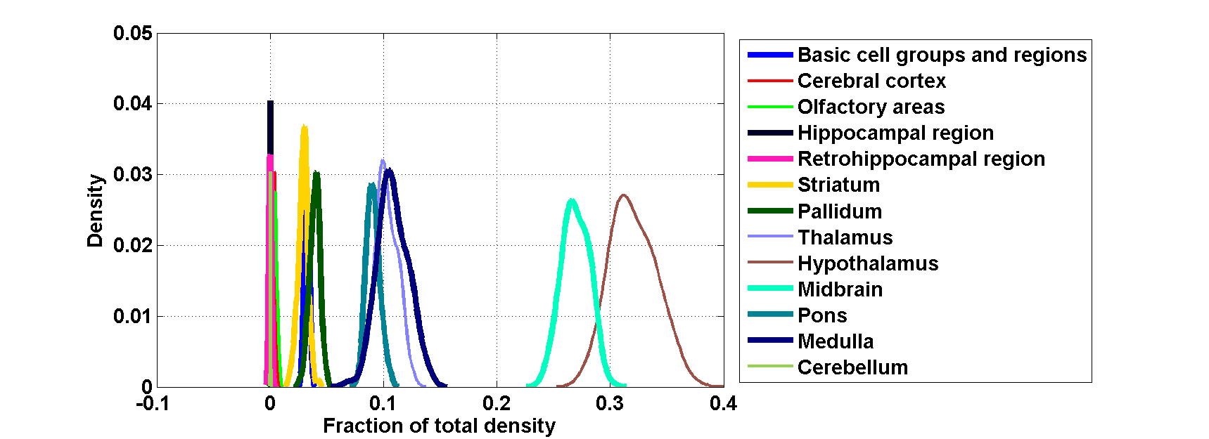
Figure 210: Distribution profiles of the density profile of cell type labeled $51$ across random sets of ISH expression energy profiles.

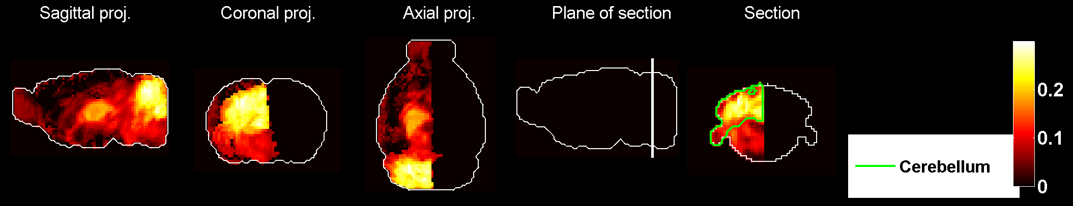
Figure 211: Heat map of the mean correlation profile for cell type labeled $52$.

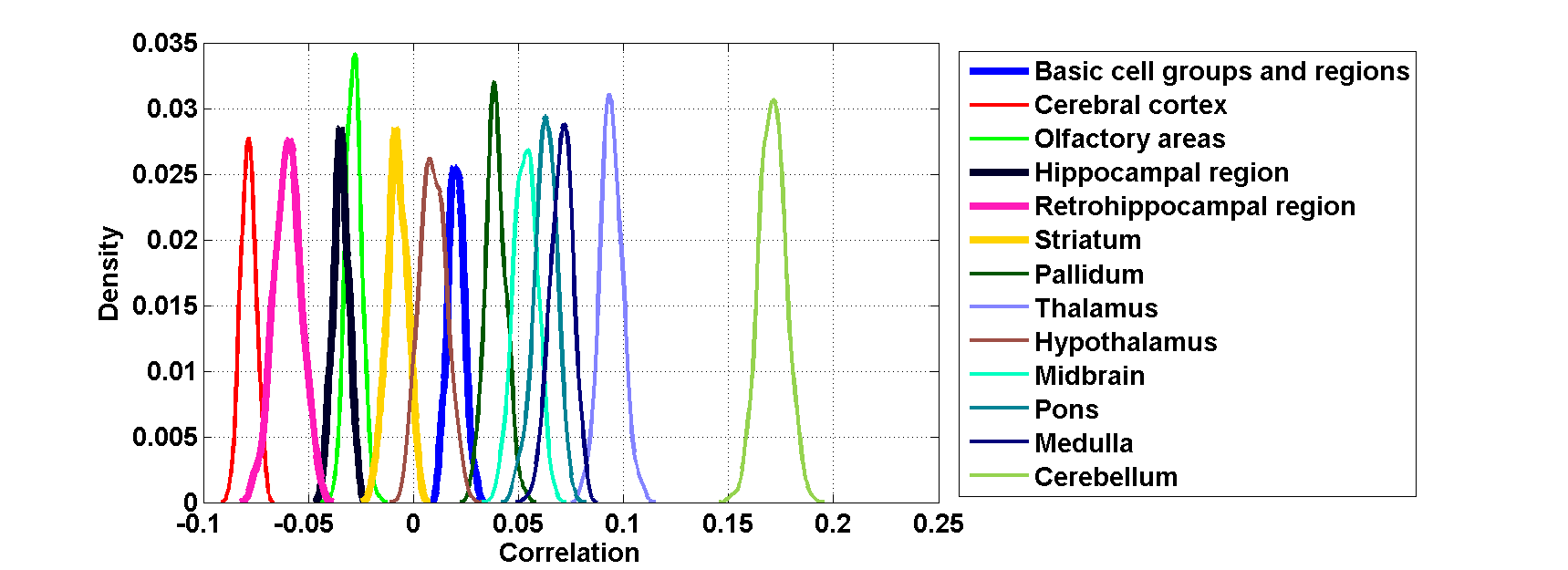
Figure 212: Distribution profiles of the correlations between transcriptome profile of cell type labeled $52$ across random sets of ISH expression energy profiles.

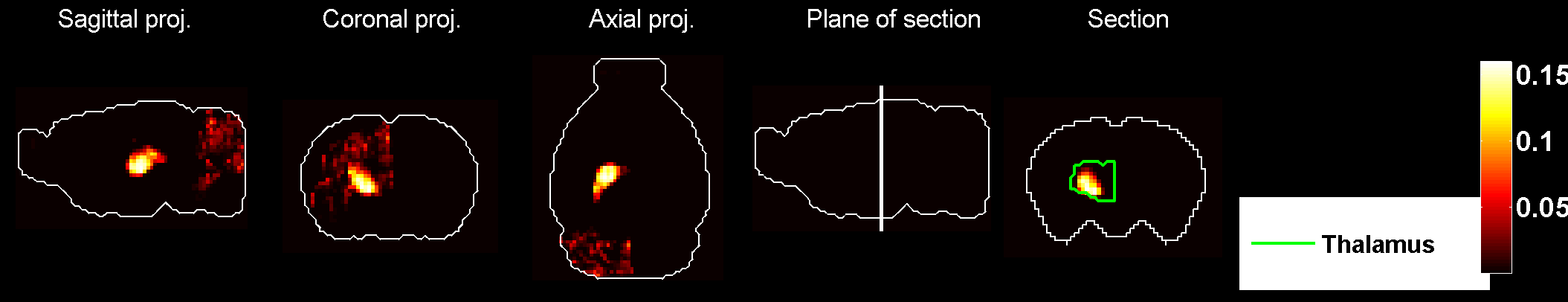
Figure 213: Heat map of the mean density profile for cell type labeled $52$.

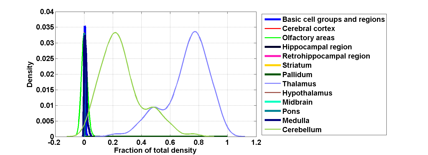
Figure 214: Distribution profiles of the density profile of cell type labeled $52$ across random sets of ISH expression energy profiles.

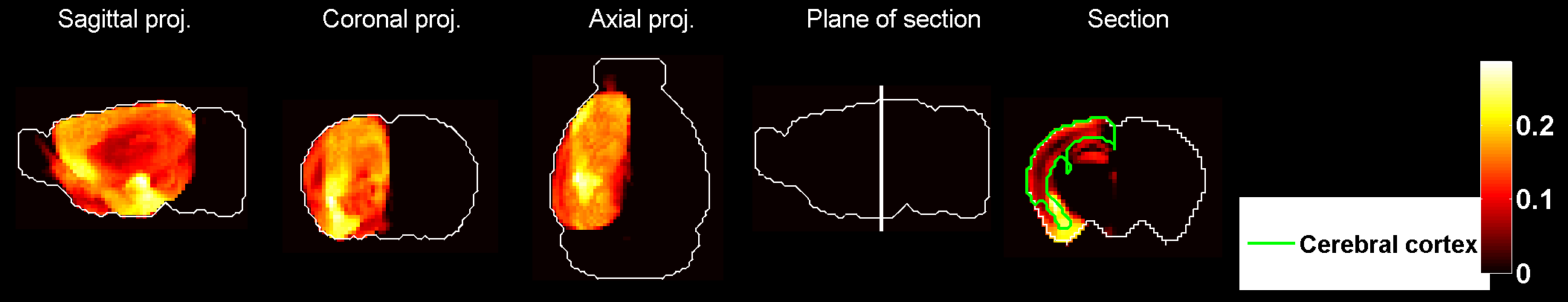
Figure 215: Heat map of the mean correlation profile for cell type labeled $53$.

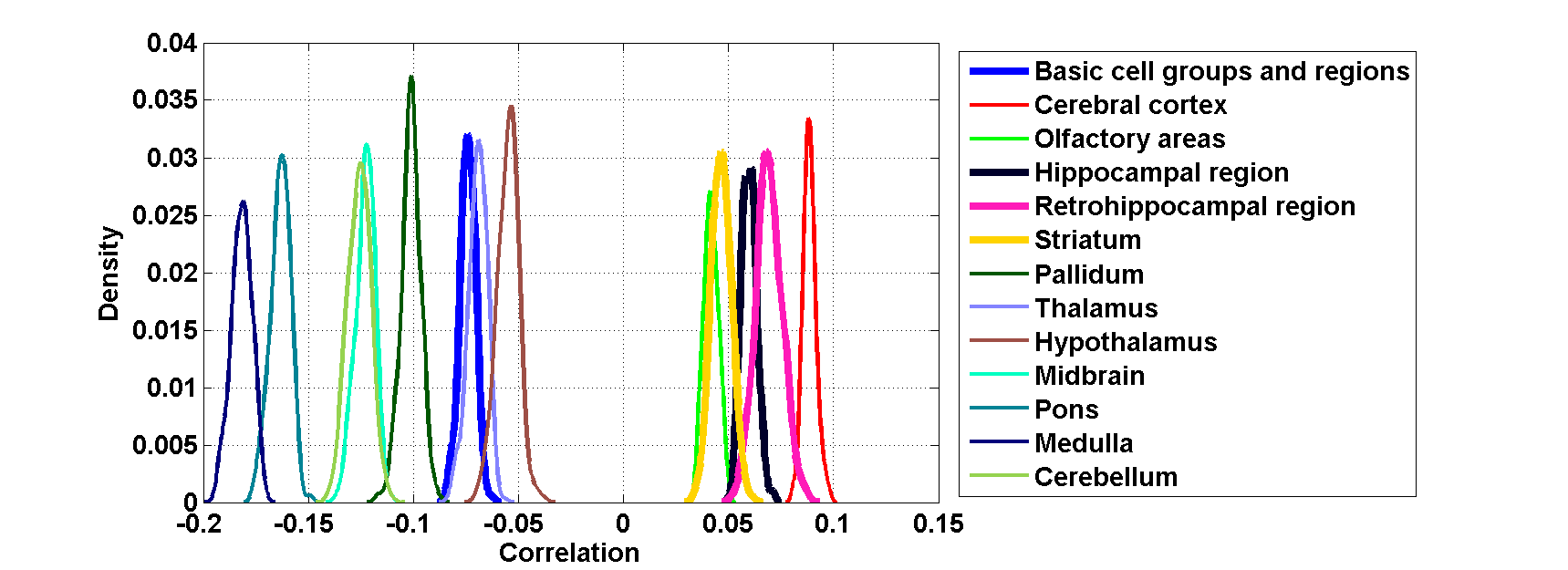
Figure 216: Distribution profiles of the correlations between transcriptome profile of cell type labeled $53$ across random sets of ISH expression energy profiles.

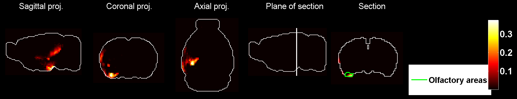
Figure 217: Heat map of the mean density profile for cell type labeled $53$.

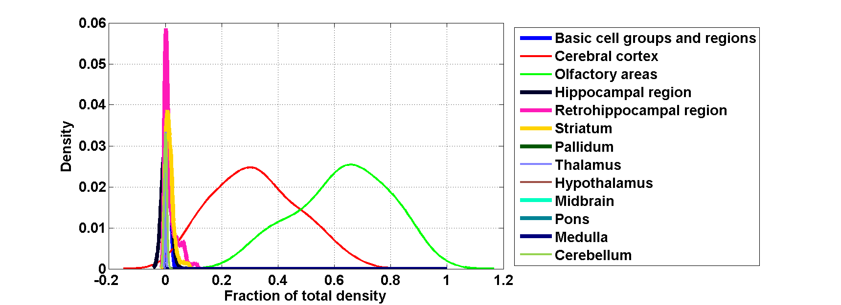
Figure 218: Distribution profiles of the density profile of cell type labeled $53$ across random sets of ISH expression energy profiles.

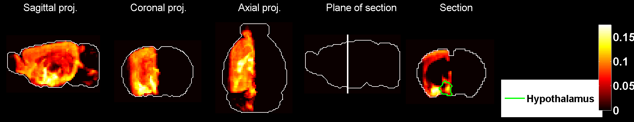
Figure 219: Heat map of the mean correlation profile for cell type labeled $54$.

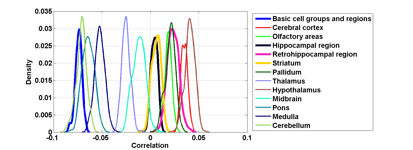
Figure 220: Distribution profiles of the correlations between transcriptome profile of cell type labeled $54$ across random sets of ISH expression energy profiles.

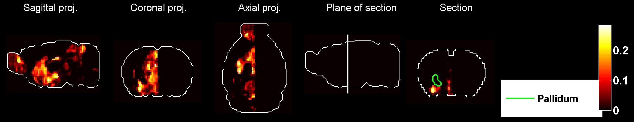
Figure 221: Heat map of the mean density profile for cell type labeled $54$.

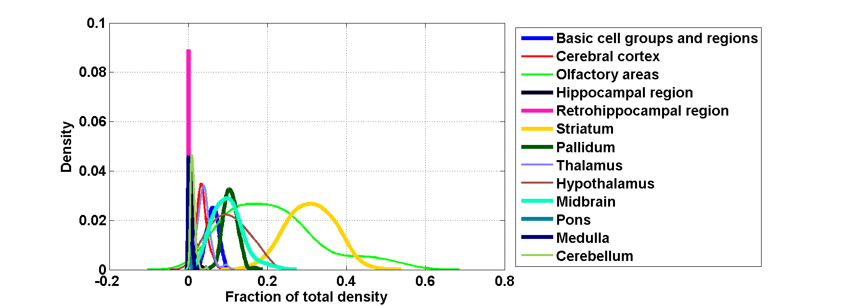
Figure 222: Distribution profiles of the density profile of cell type labeled $54$ across random sets of ISH expression energy profiles.

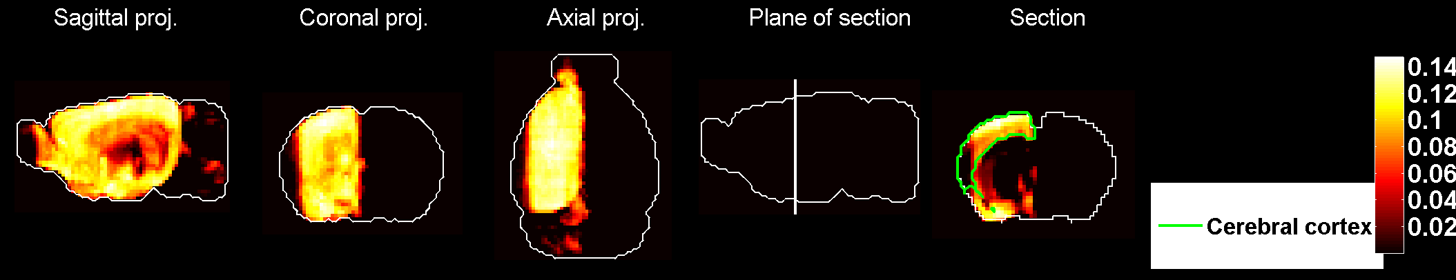
Figure 223: Heat map of the mean correlation profile for cell type labeled $55$.

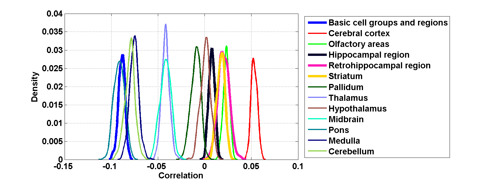
Figure 224: Distribution profiles of the correlations between transcriptome profile of cell type labeled $55$ across random sets of ISH expression energy profiles.

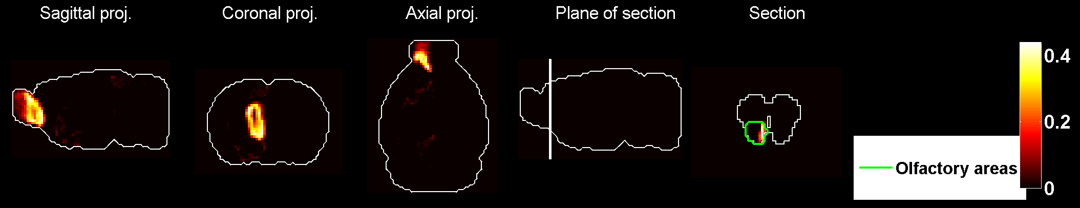
Figure 225: Heat map of the mean density profile for cell type labeled $55$.

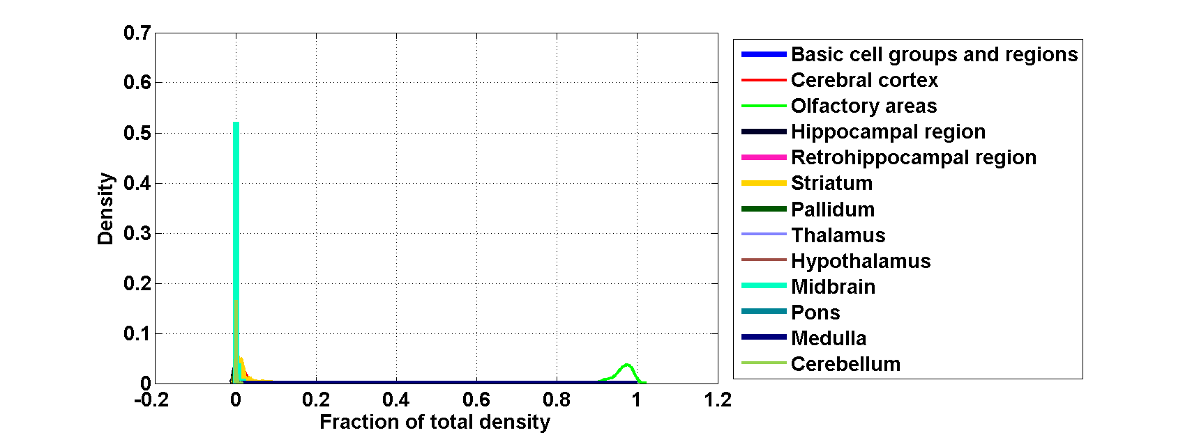
Figure 226: Distribution profiles of the density profile of cell type labeled $55$ across random sets of ISH expression energy profiles.

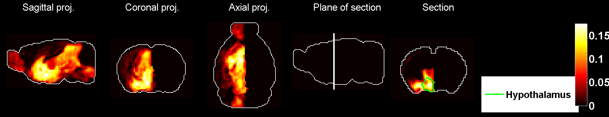
Figure 227: Heat map of the mean correlation profile for cell type labeled $56$.

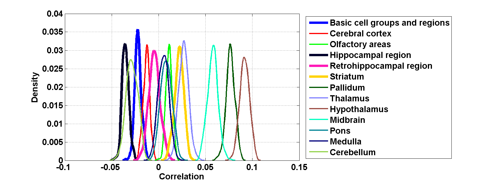
Figure 228: Distribution profiles of the correlations between transcriptome profile of cell type labeled $56$ across random sets of ISH expression energy profiles.

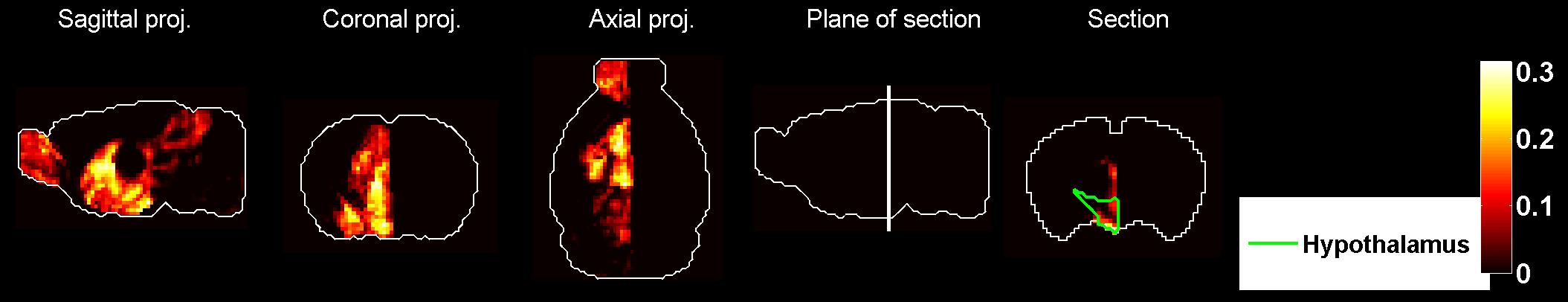
Figure 229: Heat map of the mean density profile for cell type labeled $56$.

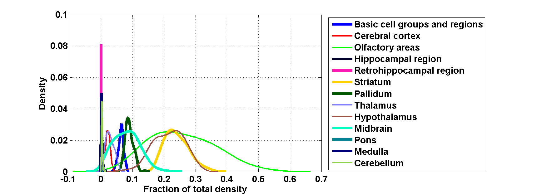
Figure 230: Distribution profiles of the density profile of cell type labeled $56$ across random sets of ISH expression energy profiles.

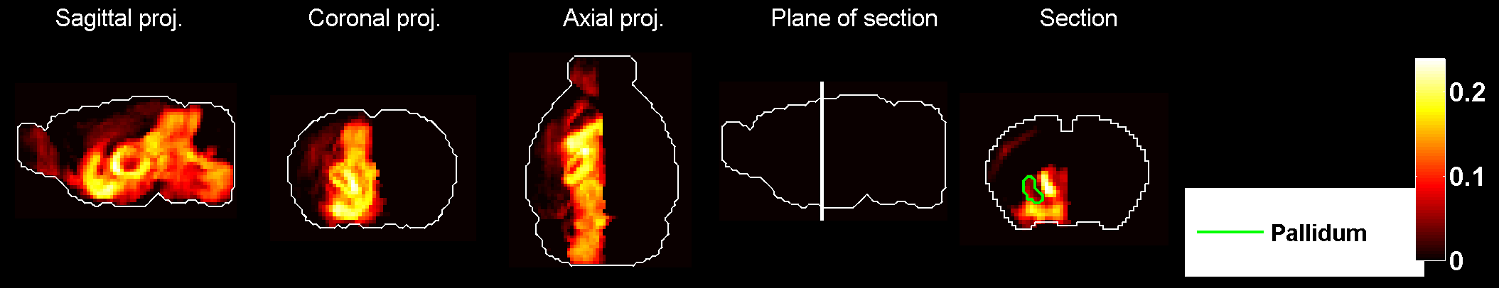
Figure 231: Heat map of the mean correlation profile for cell type labeled $57$.

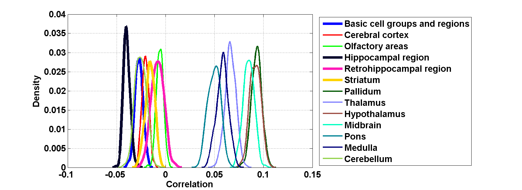
Figure 232: Distribution profiles of the correlations between transcriptome profile of cell type labeled $57$ across random sets of ISH expression energy profiles.

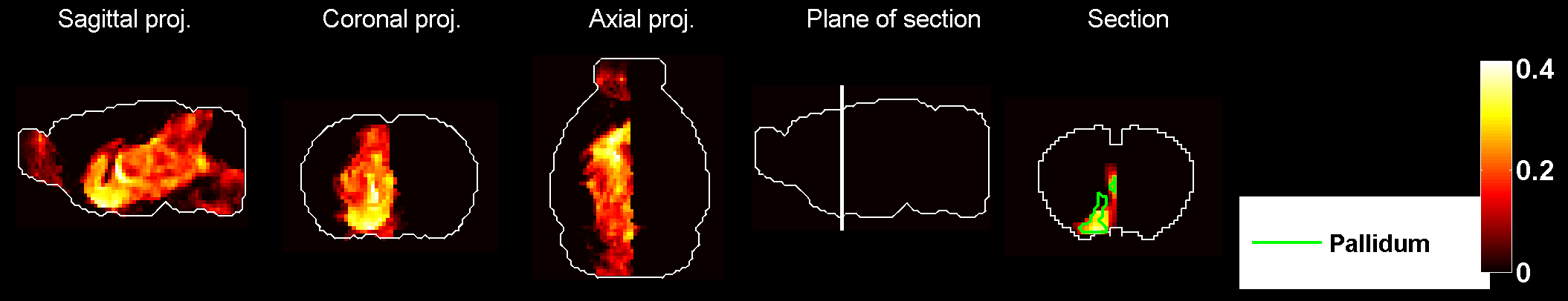
Figure 233: Heat map of the mean density profile for cell type labeled $57$.

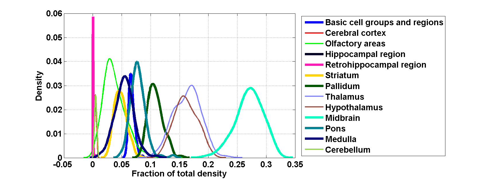
Figure 234: Distribution profiles of the density profile of cell type labeled $57$ across random sets of ISH expression energy profiles.

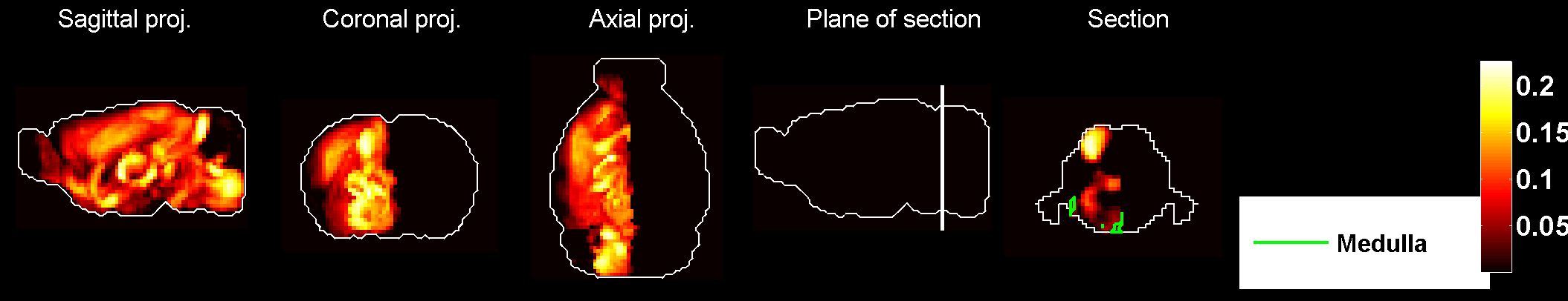
Figure 235: Heat map of the mean correlation profile for cell type labeled $58$.

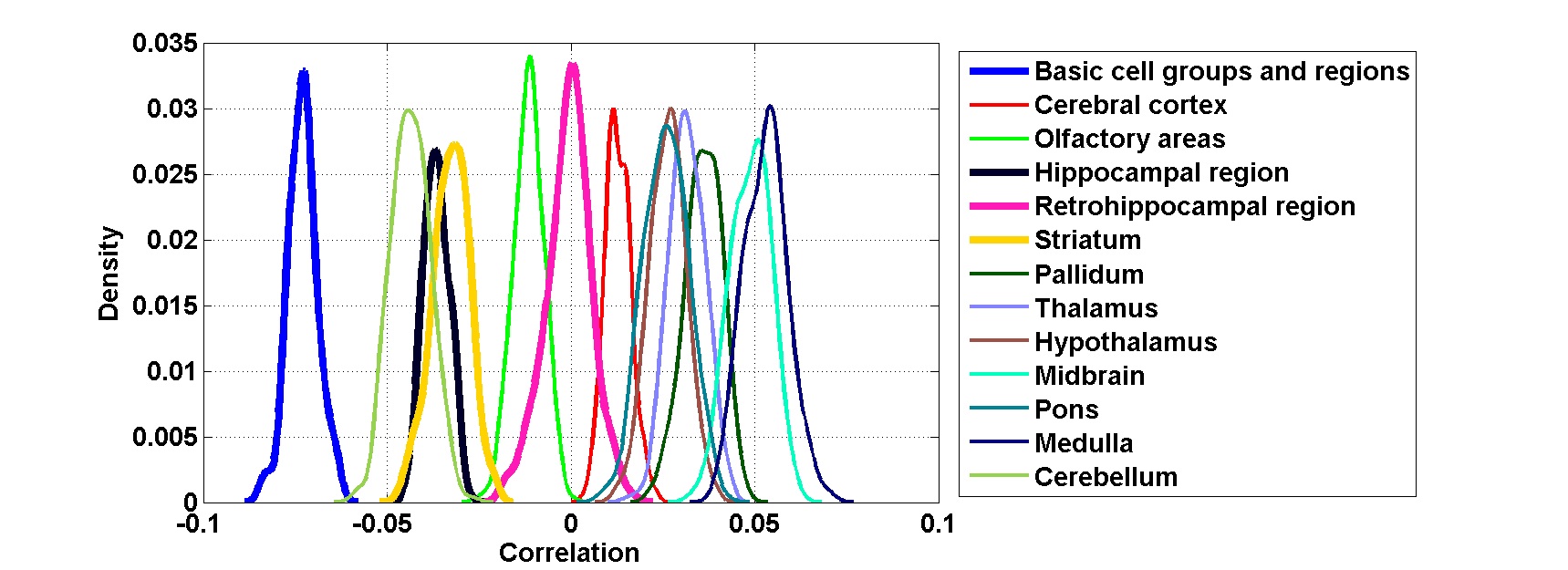
Figure 236: Distribution profiles of the correlations between transcriptome profile of cell type labeled $58$ across random sets of ISH expression energy profiles.

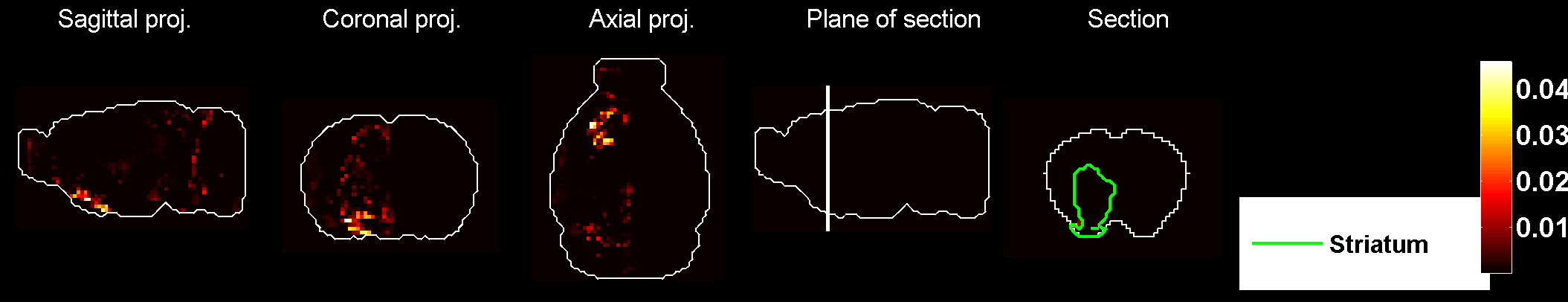
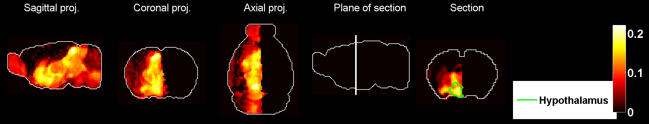
Figure 237: Heat map of the mean density profile for cell type labeled $58$.

Figure 238: Distribution profiles of the density profile of cell type labeled $58$ across random sets of ISH expression energy profiles.

Figure 239: Heat map of the mean correlation profile for cell type labeled $59$.

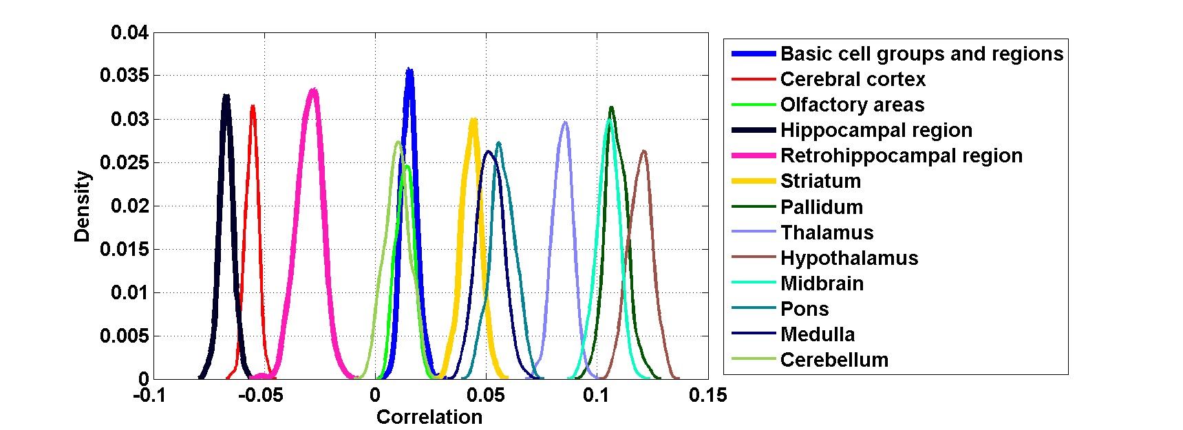
Figure 240: Distribution profiles of the correlations between transcriptome profile of cell type labeled $59$ across random sets of ISH expression energy profiles.

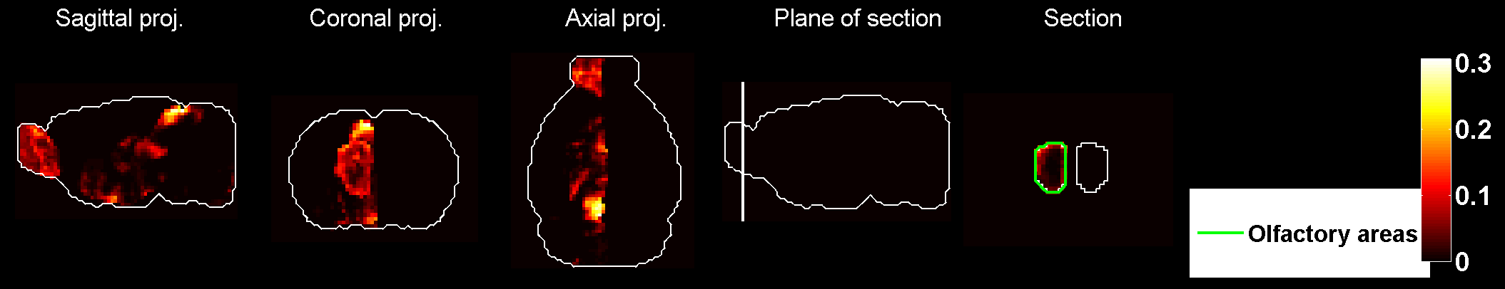
Figure 241: Heat map of the mean density profile for cell type labeled $59$.

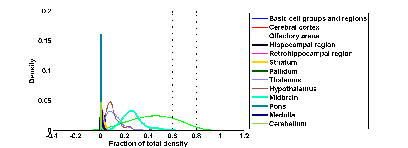
Figure 242: Distribution profiles of the density profile of cell type labeled $59$ across random sets of ISH expression energy profiles.

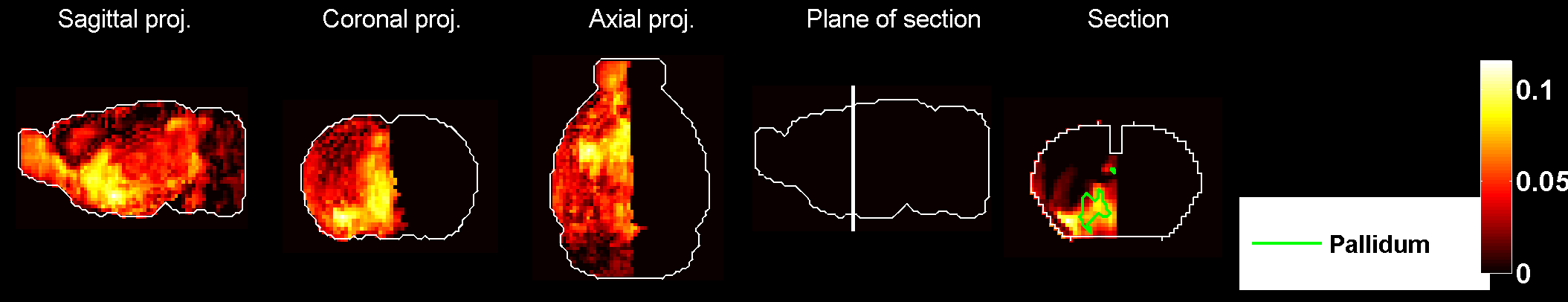
Figure 243: Heat map of the mean correlation profile for cell type labeled $60$.

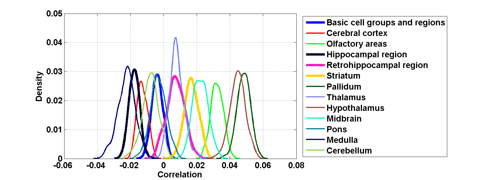
Figure 244: Distribution profiles of the correlations between transcriptome profile of cell type labeled $60$ across random sets of ISH expression energy profiles.

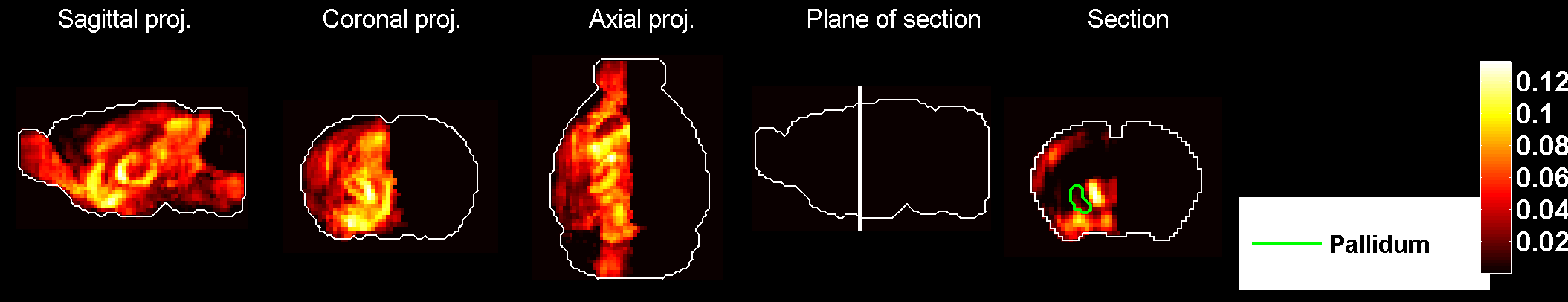
Figure 245: Heat map of the mean density profile for cell type labeled $60$.

Figure 246: Distribution profiles of the density profile of cell type labeled $60$ across random sets of ISH expression energy profiles.

Figure 247: Heat map of the mean correlation profile for cell type labeled $61$.

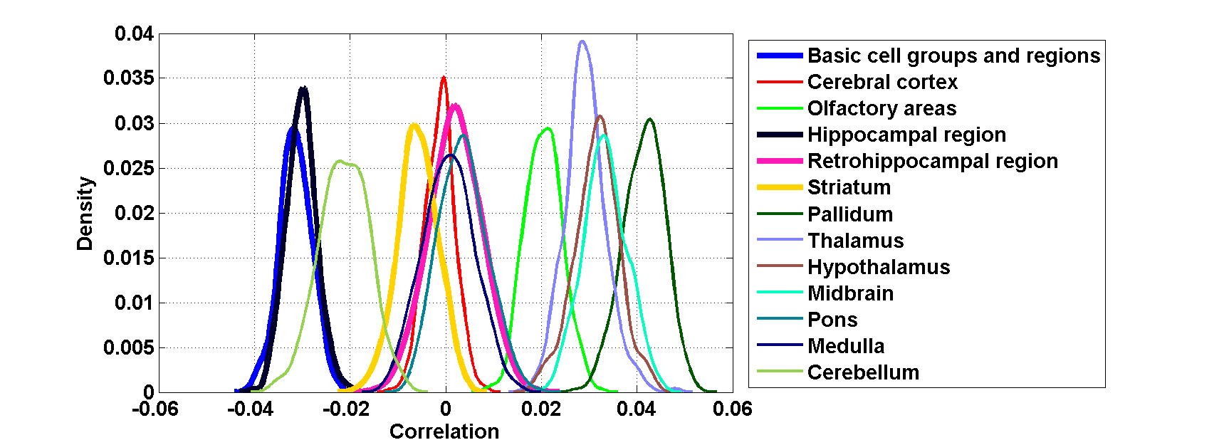
Figure 248: Distribution profiles of the correlations between transcriptome profile of cell type labeled $61$ across random sets of ISH expression energy profiles.

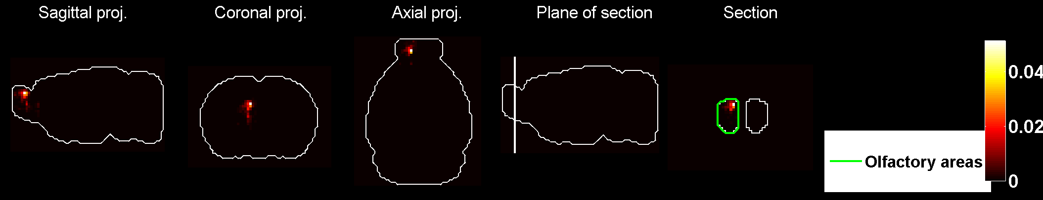
Figure 249: Heat map of the mean density profile for cell type labeled $61$.

Figure 250: Distribution profiles of the density profile of cell type labeled $61$ across random sets of ISH expression energy profiles.

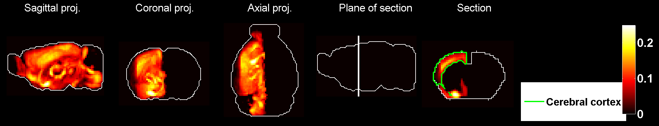
Figure 251: Heat map of the mean correlation profile for cell type labeled $62$.

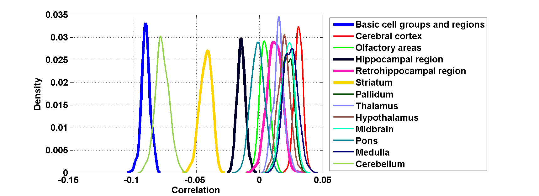
Figure 252: Distribution profiles of the correlations between transcriptome profile of cell type labeled $62$ across random sets of ISH expression energy profiles.

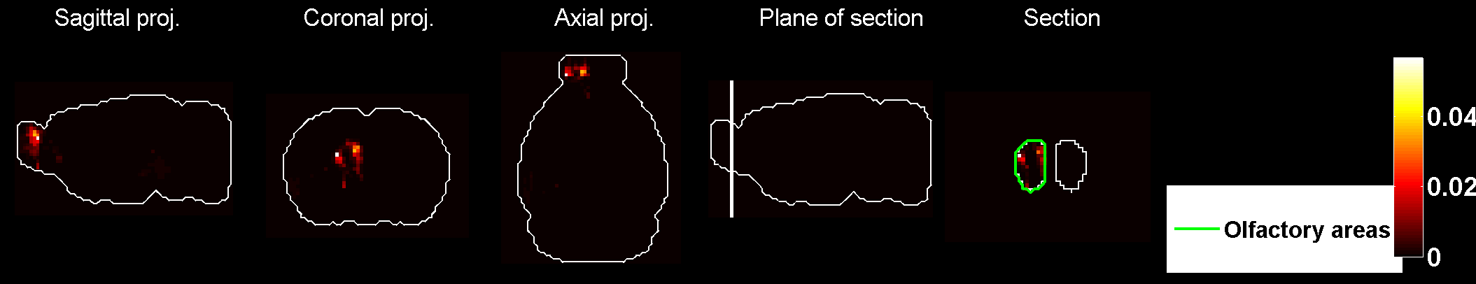
Figure 253: Heat map of the mean density profile for cell type labeled $62$.

Figure 254: Distribution profiles of the density profile of cell type labeled $62$ across random sets of ISH expression energy profiles.

Figure 255: Heat map of the mean correlation profile for cell type labeled $63$.

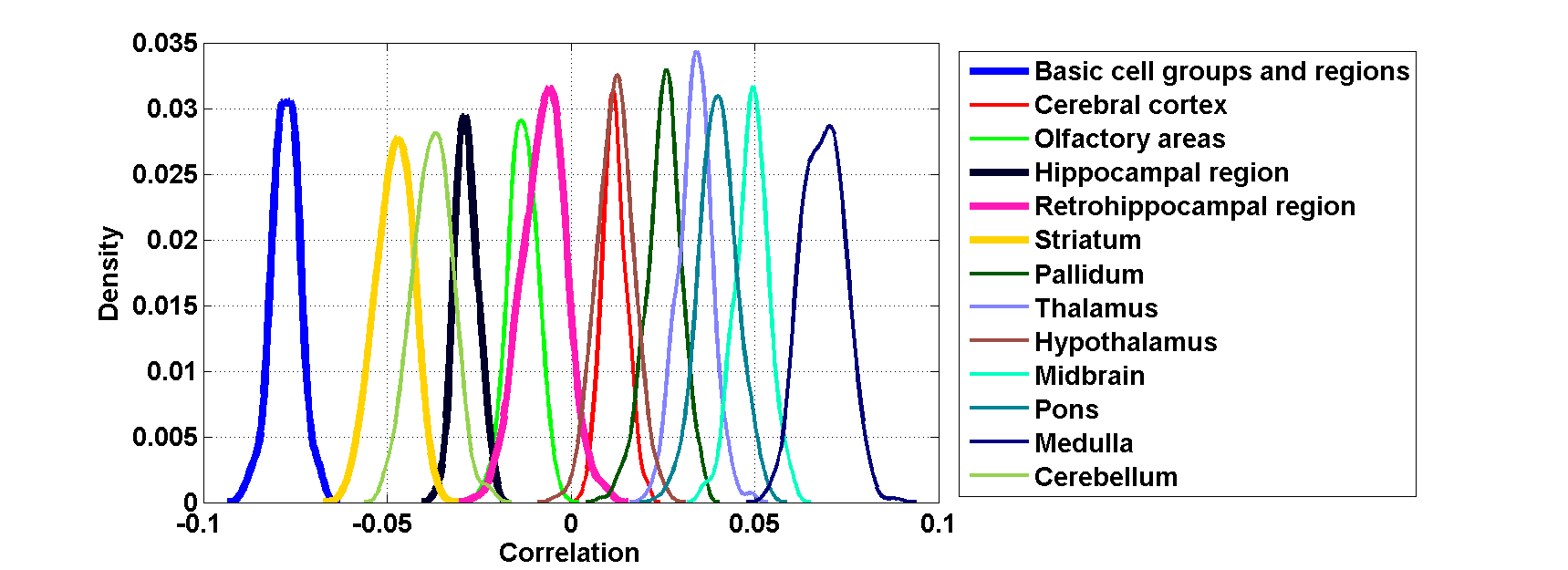
Figure 256: Distribution profiles of the correlations between transcriptome profile of cell type labeled $63$ across random sets of ISH expression energy profiles.

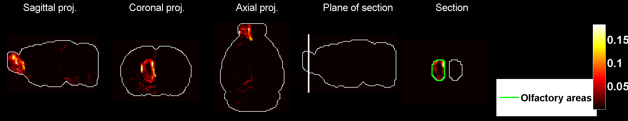
Figure 257: Heat map of the mean density profile for cell type labeled $63$.

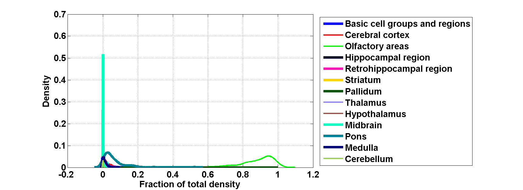
Figure 258: Distribution profiles of the density profile of cell type labeled $63$ across random sets of ISH expression energy profiles.

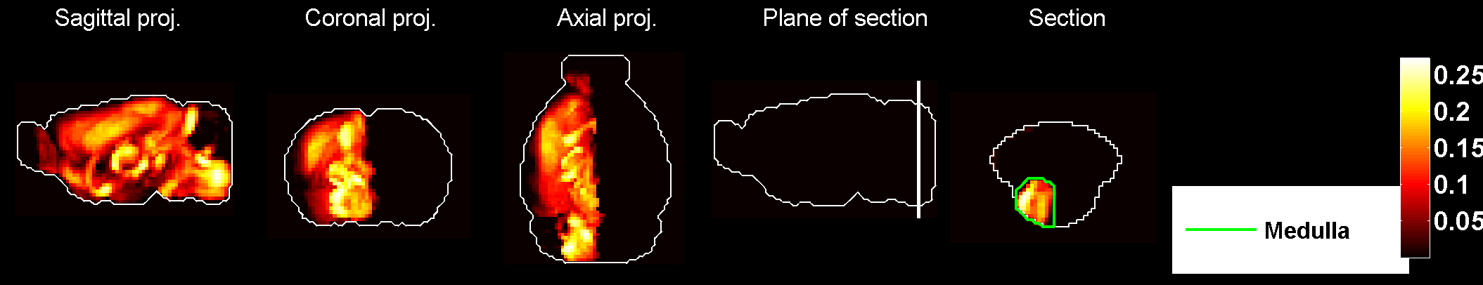
Figure 259: Heat map of the mean correlation profile for cell type labeled $64$.

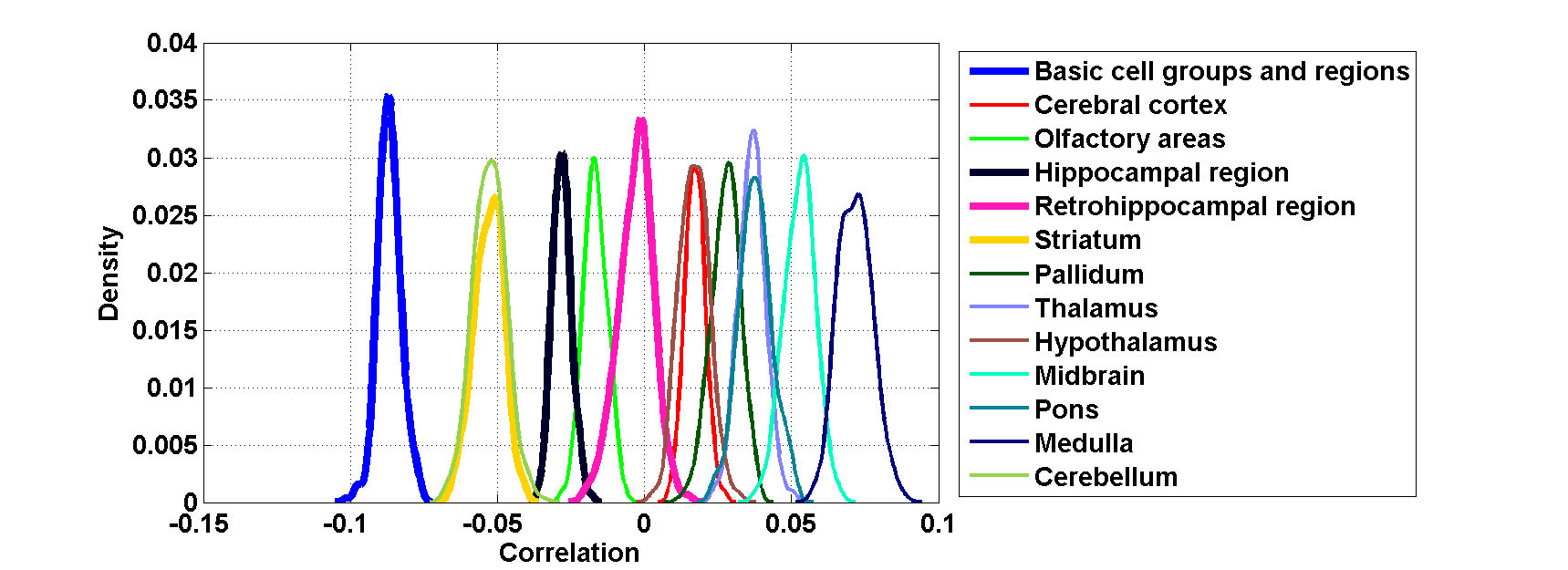
Figure 260: Distribution profiles of the correlations between transcriptome profile of cell type labeled $64$ across random sets of ISH expression energy profiles.

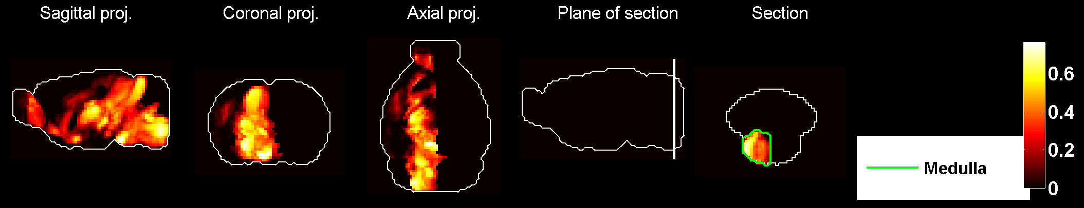
Figure 261: Heat map of the mean density profile for cell type labeled $64$.

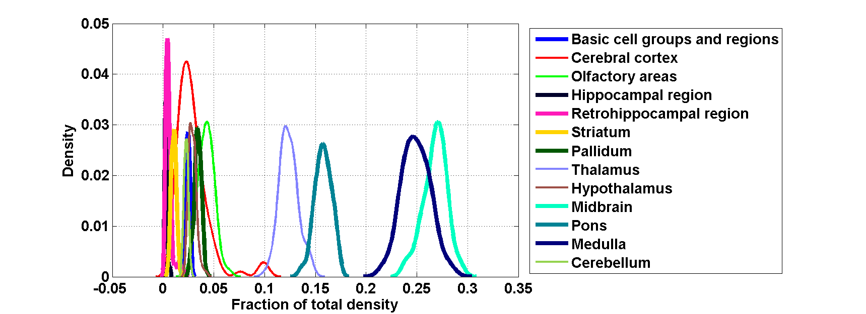
Figure 262: Distribution profiles of the density profile of cell type labeled $64$ across random sets of ISH expression energy profiles.

References

- [1] Lein ES, et al. (2007) Genome-wide atlas of gene expression in the adult mouse brain, Nature 445, 168–176.
- [2] Ng, L. et al. (2009), An anatomic gene expression atlas of the adult mouse brain, Nature Neuroscience 12, 356–362.
- [3] Hawrylycz M, et al. (2011) Multi-scale correlation structure of gene expression in the brain. Neural Networks 24 (2011) 933–942.
- [4] Dong HW (2007), The Allen reference atlas: a digital brain atlas of the C57BL/6J male mouse, Wiley.
- [5] Grange P, Hawrylycz M, Mitra PP (2013), Computational neuroanatomy and co-expression of genes in the adult mouse brain, analysis tools for the Allen Brain Atlas. Quantitative Biology, 1(1): 91–100. (DOI) 10.1007/s40484-013-0011-5.
- [6] Menashe I, Grange P, Larsen EC, Banerjee-Basu S, Mitra PP (2013). Co-expression profiling of autism genes in the mouse brain. PLoS Comput. Biol. 9(7): e1003128.
- [7] Grange, P., Menashe, I. and Hawrylycz, M. (2015). Cell-type-specific neuroanatomy of cliques of autism-related genes in the mouse brain. Frontiers in Computational Neuroscience, 9, 55.
- [8] Grange, P., Bohland, J. W., Hawrylycz, M. and Mitra, P. P. (2012). Brain Gene Expression Analysis: a MATLAB toolbox for the analysis of brain-wide gene-expression data. arXiv preprint arXiv:1211.617.
- [9] Grange P, Mitra PP (2012) Computational neuroanatomy and gene expression: optimal sets of marker genes for brain regions. IEEE, in CISS 2012, 46th annual conference on Information Science and Systems (Princeton).
- [10] Bohland JW et al. (2010) Clustering of spatial gene expression patterns in the mouse brain and comparison with classical neuroanatomy, Methods, 50(2), 105–112.
- [11] Sugino K et al. (2005), Molecular taxonomy of major neuronal classes in the adult mouse forebrain. Nature Neuroscience 9, 99–107.
- [12] Chung CY et al. (2005), Cell-type-specific gene expression of midbrain dopaminergic neurons reveals molecules involved in their vulnerability and protection. Hum. Mol. Genet. 14: 1709–1725.
- [13] Arlotta P, et al. (2005), Neuronal subtype-specific genes that control corticospinal motor neuron development in vivo. Neuron 45: 207–221.
- [14] Rossner MJ, et al. (2006), Global transcriptome analysis of genetically identified neurons in the adult cortex. J. Neurosci. 26(39) 9956–66.
- [15] Heiman M, et al. (2008) A translational profiling approach for the molecular characterization of of CNS cell types. Cell 135: 738–748.
- [16] Cahoy JD, et al. (2008), A transcriptome database for astrocytes, neurons, and oligodendrocytes: a new resource for understanding brain development and function. J. Neurosci., 28(1) 264–78.
- [17] Doyle JP et al. (2008), Application of a translational profiling approach for the comparative analysis of CNS cell types. Cell 135(4) 749–62.
- [18] Okaty BW, et al. (2009), Transcriptional and electrophysiological maturation of neocortical fast-spiking GABAergic interneurons. J. Neurosci. (2009) 29(21) 7040–52.
- [19] Hawrylycz M, et al. (2011) Multi-scale correlation structure of gene expression in the brain. Neural Networks 24 (2011) 933–942.
- [20] Grange P, Bohland JW, Okaty BW, Sugino K, Bokil H, Nelson SB, Ng L, Hawrylycz M, Mitra PP, Cell-type–based model explaining coexpression patterns of genes in the brain, PNAS 2014 111 (14) 5397–5402.
- [21] P. Grange, M. Hawrylycz, P.P. Mitra, Cell-type-specific microarray data and the Allen atlas: quantitative analysis of brain-wide patterns of correlation and density, [arXiv:1303.0013].
- [22] Grange P, Bohland JW, Okaty B, Sugino K, Bokil H, Nelson S, Ng L, Hawrylycz M, Mitra PP, Cell-type-specific transcriptomes and the Allen Atlas (II): discussion of the linear model of brain-wide densities of cell types, [arXiv:1402.2820] .
- [23] Ko Y, Ament SA, Eddy JA, Caballero J, Earls JC, Hood L, Price ND (2013) Cell-type-specific genes show striking and distinct patterns of spatial expression in the mouse brain. Proceedings of the National Academy of Sciences, 110(8), 3095–3100.
- [24] Dong HW (2007), The Allen reference atlas: a digital brain atlas of the C57BL/6J male mouse, Wiley.
- [25] Okaty BW, Sugino K, Nelson SB (2011) A Quantitative Comparison of Cell-Type-Specific Microarray Gene Expression Profiling Methods in the Mouse Brain. PLoS One 6(1).
- [26] Ji, S. (2013). Computational genetic neuroanatomy of the developing mouse brain: dimensionality reduction, visualization, and clustering. BMC bioinformatics, 14(1), 222.
- [27] Ji, S., Zhang, W., Li, R. (2014). A Probabilistic Latent Semantic Analysis Model for Co-Clustering the Mouse Brain Atlas.
- [28] Tan PPC, French L, Pavlidis P (2013) Neuron-enriched gene expression patterns are regionally anti-correlated with oligodendrocyte-enriched patterns in the adult mouse and human brain. Frontiers in Neuroscience, 7.
- [29] Meinshausen N (2013) Sign-constrained least squares estimation for high-dimensional regression. Electronic Journal of Statistics, 7, 1607–1631.