Real-Space Renormalization Group for Spectral Properties of Hierarchical Networks

Abstract

We derive the determinant of the Laplacian for the Hanoi networks and use it to determine their number of spanning trees (or graph complexity) asymptotically. While spanning trees generally proliferate with increasing average degree, the results show that modifications within the basic patterns of design of these hierarchical networks can lead to significant variations in their complexity. To this end, we develop renormalization group methods to obtain recursion equations from which many spectral properties can be obtained. This provides the basis for future applications to explore the physics of several dynamic processes.

I Introduction

Understanding the dynamics of hierarchical systems is rapidly becoming a subject of wide interest within the study of complex networks Trusina et al. (2004); Clauset et al. (2008); Fischer et al. (2008); Boettcher et al. (2008a); Hasegawa and Nemoto (2013). This may seem surprising, as hierarchies are not a new subject in complexity Simon (1962), and considering that the ultimate hierarchical system – a tree – has long been studied in many variations and for many types of dynamics because exact results can be obtained. Known as Bethe approximation in statistical physics Pathria (1996); Mézard and Montanari (2006), trees locally resemble sparse mean-field models in physics, due to their infinite dimensionality. Beyond the mean-field statistical models, however, there exists a much richer dynamics arises from peculiar structural features of hierarchical networks such as high degree of clustering and modularity. In many realistic situations, such hierarchies are embedded in some finite-dimensional space Dorogovtsev et al. (2008); Barthelemy (2011), which can lead to an entirely new set of phenomena. Examples of such embedded hierarchical systems contain transport and control systems, they have been observed in the brain Moretti and Muñoz (2013); Meunier et al. (2009), or they have been studied for their novel synthetic critical behavior Hinczewski and Berker (2006); Boettcher et al. (2009); Boettcher and Brunson (2011, 2015); Nogawa et al. (2012), such as explosive transitions that are purely induced by the geometry in percolation Boettcher et al. (2012) or synchronization Li and Boettcher (in preparation). Recently, hierarchical networks based on Dyson’s model have shown to allow for the existence of a number of metastable states, which can be used to study the modular architecture and parallel processing in neuron networks as well as the ergodicity breakdown for the stochastic process Agliari et al. (2015a, b, c).

Key to understanding the mechanisms at the core of those novel phenomena lies within the geometry of these hierarchies. These geometric properties are inevitably tied to spectral properties of their network Laplacians Biggs (1974). Here, we investigate a recently proposed class of hierarchical networks Boettcher et al. (2008a) within the simplest of spatial embeddings – a simple line – for which we can obtain many spectral properties exactly using the renormalization group (RG) Pathria (1996).For these Hanoi networks, we study some basic properties of their Laplacians. In particular, we derive sets of recursion relations that allow to study their secular equations (also called characteristic polynomials), whose zeros provide all eigenvalues, to arbitrary accuracy. We determine the asymptotic scaling of their determinants with system size. These determinants can be used as a generator for many other asymptotic properties.

The Laplacian matrix is given by

$$\mathbf{L}_{i,j} = d_{i}\delta_{i,j}-A_{i,j},$$ (1)

where $d_{i}$ specifies the degree of the $i$-th site and $A_{i,j}$ is the adjacency matrix of the network. Since we assume that the links in the networks are undirected, ${\bf A}$, and hence ${\bf L}$, are symmetric. We further assume that there are no external links, which implies the vanishing of all row or column sums in ${\bf L}$, $\sum_{i}\mathbf{L}_{i,j}=\sum_{j}\mathbf{L}_{i,j}=0$. The fundamental property characterizing the Laplacian matrix is its spectrum of eigenvalues, the solutions $\lambda_{i}$ of the secular equation

$$\det\left[{\bf L}-\lambda{\bf 1}\right] = 0.$$ (2)

This spectrum is highly nontrivial for the Hanoi networks, and we will not be able to describe it in much detail here. But we can provide an RG approach that reduces the effort exponentially from solving $2^{k}\times 2^{k}$ determinants to $k$ iterations of a closed set of RG recursion equations for any desired quantity, where $N=2^{k}$ refers to the number of sites in the network. Numerous aspects can be extracted in closed form asymptotically.

The spectrum of network Laplacians features in many practical applications. The scaling of the ratio between largest and smallest eigenvalue indicates the synchronizability of a network Barahona and Pecora (2002), which also can be approximated by a sum over all eigenvalues (inverted) when related to a random deposition process Korniss et al. (2003); Boettcher (2012). Permeability and well-connectedness of networks can be defined in terms of their smallest eigenvalue Maas (1987). The spectrum further features prominently in quantum transport Boettcher et al. (2011),the behavior of continuous-time quantum search algorithms Childs and Goldstone (2004); Agliari et al. (2010), graph partitioning Pothen et al. (1990); Hendrickson and Leland (1995) and image processing Peinecke et al. (2007), just to name a few examples. Of course, Laplacian spectra also determine the characteristic frequencies of mechanical vibrations, from which connectivity between interacting units within the membrane can be identified Fisher (1966). Thus, there has long been strong motivation to study such spectra particularly on fractal networks, where its properties can be explored in great detail Domany et al. (1983); Rammal (1984); Fukushima and Shima (1992); Rammal and Toulouse (1983); Shima (1991); Teplyaev (2000).

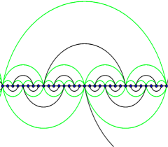
Figure 1: Depiction of the Hanoi networks HN3 and HN5. The 3-regular network HN3 corresponds to the solid (black) lines alone, while HN5 in addition also consists of the (green-) shaded lines. For HN5, sites on the lowest level of the hierarchy have degree 3, then degree 5, 7, etc, concerning a fraction of 1/2, 1/4, 1/8, etc., of all sites, which makes for an average degree 5 in this network. Note that both networks are planar.

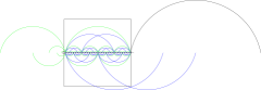
Figure 2: Depiction of the nonplanar Hanoi networks HNNP and HN6. Again, starting from a 1d-backbone (black lines), in HNNP a set of long-range links (blues-shades lines) is added that break planarity but maintain the hierarchical pattern set out in Eq. (5) that leads to a network of average degree 4. If we add again the same links that distinguished HN3 and HN5 in Fig. 1, we obtain HN6 with average degree 6. In all cases, the RG on these networks remains exact.

Here, we will only focus on the simplest case of the scaling of the determinant itself, obtained by taking $\lambda\to 0$ in Eq. (2), which provides the number of spanning trees,

$$\#_{{\rm ST}}=-\lim_{\lambda\to 0}\frac{\det\left[{\bf L}-\lambda{\bf 1}\right]}{\lambda N},$$ (3)

sometimes also referred to as “graph complexity” Lyons (2005). Eq. (3) is one of the oldest results in algebraic graph theory, due to Kirchhoff (1847) Biggs (1974). Spanning trees describe the size of the attractor state in the self-organized critical sandpile model Dhar (1999), they characterize the optimal paths between any two sites in a network Wu et al. (2006), and are also related to optimal synchronizability of a network Nishikawa and Motter (2006). The number of spanning trees is of fundamental interest in mathematics and physics. For example, it is related to the partition function of $q$-state Potts model in the limit $q\rightarrow 0$ Dhar (1977); Wu (1982) Thus, studies on the asymptotic growth of spanning trees are well motivated not only for regular lattices Shrock and Wu (2000), but also on self-similar structures Chang et al. (2007); Teufl and Wagner (2006, 2011). On these networks, the number of spanning trees $\#_{ST}$ exponentially increases with $N$, which can be characterized by the tree entropy, which is the entropy-density of spanning trees Lyons (2005); Chang et al. (2007); Teufl and Wagner (2010),

$$s = \lim_{N\rightarrow\infty}\frac{\ln\left(\#_{{\rm ST}}\right)}{N}.$$ (4)

The number of spanning trees on Hanoi networks can be easily derived from our RG procedure, allowing us to explore the role of geometric structures on its asymptotic growth.

II Structure of Hierarchical Networks

The Hanoi networks we discuss in this paper were introduced first in Ref. Boettcher et al. (2008a). Each of the networks considered in this paper possesses a simple geometric backbone, a one-dimensional line of sites $N$. in which each site is at least connected to its nearest neighbor left and right on the backbone. To generate the small-world hierarchy in these networks, consider parameterizing any number $n>0$ uniquely in terms of two other integers $(i,j)$, $i\geqslant 1$ and $1\leqslant j\leqslant 2^{k-i}$, via

$$n = 2^{i-1}\left(2j-1\right),$$ (5)

which motivated the name of the networks .

The networks can be considered either closed into a loop of $N=2^{k}$ sites or in a linear arrangement with $N=2^{k}+1$ sites, a difference that typically does not effect the RG and any leading asymptotic property. Their recursive pattern is far more easily to illustrate when drawn linearly, as for HN3 and HN5 in Fig. 1 and for HNNP and HN6 in Fig. 2, although in our calculations we avoid spurious edge-effects by considering periodic loops, where sites $n=0$ and $n=N=2^{k}$ are identical to each other. For convenient comparisons, we call the ordinary one-dimensional loop HN2 (for Hanoi Network of degree 2). The details of the design and most of their geometric properties have been discussed at length elsewhere Boettcher and Brunson (2011).

III Obtaining the RG-Recursions

In this Section, we show how to obtain the recursion equations for the RG-flow of our networks that describes the asymptotic properties of the lattice Laplacian. To that end, we employ the well-known formal identity Ramond (1997),

$$\frac{1}{\sqrt{\det L_{k}^{(\alpha)}}} = \dotsintop_{-\infty}^{\infty}\left(\prod_{i=n}^{N}\frac{dx_{n}}{\sqrt{\pi}}\right)\exp\left\{-\sum_{n=1}^{N}\sum_{m=1}^{N}x_{n}\left(L_{k}^{(\alpha)}\right)_{n,m}x_{m}\right\},$$ (6)

for the evaluation of the determinant of $L_{k}^{(\alpha)}$ for each network HN$\alpha$ with $\alpha\in\left\{2,3,5,NP,6\right\}$ of size $N=2^{k}$. (Since Laplacians are singular matrices, formally, some integrals will not converge and need regulation, however, these singularities will be dealt with explicitly below in the final step of the RG.) We can group our networks into two classes of equivalent topologies, as respectively Figs. 1 and 2 suggest: HN3 is contained within HN5 and HNNP is contained within HN6, while the simple loop (HN2) is contained within both, of course. In addition, removing the backbone of HNNP decomposes it into three separate, loop-less tree structures that have been studied in Ref. Hasegawa and Nogawa (2013).

The following calculations are purely formal, as some of the integrals may not converge in Eq. (6), in which case we would have to insert some form of regulation. Yet, the integrals merely serve as generators for the desired RG-recursions, essentially. Alternative algebraic means to evaluate the determinants that do not involve integrals have been used for a specific application previously Domany et al. (1983); Boettcher et al. (2011). However, the approach taken here provides entirely equivalent results with a clearer perspective on the topological transformations that are involved. Furthermore, the current approach is closely linked to the description of a path-integral for a free field-theory Ramond (1997) on a given network, which affords certain extensions of the methods, for example, by inserting source-terms $\sum_{n=1}^{N}J_{n}x_{n}$ into the exponential in Eq. (6) as generators for more complicated observables. When these sources are either uniform ($J_{n}\equiv J$ f.a. $n$), localized ($J_{n}=J\delta_{n,x}$), or hierarchically staggered [$J_{n}=J_{i(n)}$ according to Eq. (5)], exact RG-recursions may still be obtained.

III.1 Renormalization Group calculation for the determinant of HN3 and HN5

Here, we evaluate the most general $2^{k}\times 2^{k}$-determinant for the matrix $L_{k}^{(\alpha)}$ that is used in the analysis of HN3 and HN5 (and HN2) below. The properties of each determinant emerges via renormalization from $L_{k}^{(\alpha)}$ for a different set of “bare” parameters, while the RG-recursions themselves remain the same for each $\alpha\in\left\{2,3,5\right\}$. These parameters describing the renormalized weights of effective links between sites, while their bare values serve as initial conditions on these RG recursion equations. We define $L_{k}^{(2)}$ as the matrix of a one-dimensional loop of $2^{k}$ sites (which we may call HN2). $L_{k}^{(3)}$ and $L_{k}^{(5)}$ are respectively the matrices for the HN3 and HN5 networks. Instead of providing a formal description of $L_{k}^{(\alpha)}$ for general size $2^{k}$, we simply illustrate its generic recursive pattern for the case $k=4$:

$$L_{k=4}^{(3,5)} = \left[\begin{array}[]{cccccccccccccccc}q_{4}&-p_{0}&-l_{1}&0&-l_{2}&0&0&0&-2l_{3}&0&0&0&-l_{2}&0&-l_{1}&-p_{0}\\ -p_{0}&q_{1}&-p_{0}&-p_{1}&0&0&0&0&0&0&0&0&0&0&0&0\\ -l_{1}&-p_{0}&q_{2}&-p_{0}&-l_{1}&0&-p_{2}&0&0&0&0&0&0&0&0&0\\ 0&-p_{1}&-p_{0}&q_{1}&-p_{0}&0&0&0&0&0&0&0&0&0&0&0\\ -l_{2}&0&-l_{1}&-p_{0}&q_{3}&-p_{0}&-l_{1}&0&-l_{2}&0&0&0&-p_{3}&0&0&0\\ 0&0&0&0&-p_{0}&q_{1}&-p_{0}&-p_{1}&0&0&0&0&0&0&0&0\\ 0&0&-p_{2}&0&-l_{1}&-p_{0}&q_{2}&-p_{0}&-l_{1}&0&0&0&0&0&0&0\\ 0&0&0&0&0&-p_{1}&-p_{0}&q_{1}&-p_{0}&0&0&0&0&0&0&0\\ -2l_{3}&0&0&0&-l_{2}&0&-l_{1}&-p_{0}&q_{4}&-p_{0}&-l_{1}&0&-l_{2}&0&0&0\\ 0&0&0&0&0&0&0&0&-p_{0}&q_{1}&-p_{0}&-p_{1}&0&0&0&0\\ 0&0&0&0&0&0&0&0&-l_{1}&-p_{0}&q_{2}&-p_{0}&-l_{1}&0&-p_{2}&0\\ 0&0&0&0&0&0&0&0&0&-p_{1}&-p_{0}&q_{1}&-p_{0}&0&0&0\\ -l_{2}&0&0&0&-p_{3}&0&0&0&-l_{2}&0&-l_{1}&-p_{0}&q_{3}&-p_{0}&-l_{1}&0\\ 0&0&0&0&0&0&0&0&0&0&0&0&-p_{0}&q_{1}&-p_{0}&-p_{1}\\ -l_{1}&0&0&0&0&0&0&0&0&0&-p_{2}&0&-l_{1}&-p_{0}&q_{2}&-p_{0}\\ -p_{0}&0&0&0&0&0&0&0&0&0&0&0&0&-p_{1}&-p_{0}&q_{1}\end{array}\right].$$ (23)

The bare parameters $q_{i}$ on the diagonal refer to on-site properties of each site $n$ that belongs to the $i$-th hierarchy as determined by Eq. (5). For the case of the lattice Laplacian here, for example, $q_{i}$ is simply the degree of that site. The off-diagonal parameters label extant or potentially emerging links between sites that are undirected, so the matrix is symmetric. To keep parameters fundamentally non-negative, we insert negative signs explicitly, so that the bare values for all $p_{i}$ is uniformly unity, however, they renormalize differently for each $i$. (Here, level $i=0$ refers to nearest-neighbor links in the backbone.) While the $p_{i}$ correspond to the solid black lines in Fig. 1, the parameters $l_{i}$ refer to those long-range links shaded in green in Fig. 1, whose addition make up HN5. (Entries like $-2l_{k-1}$ near the highest level of the hierarchy correspond to a convenient choice in imposing periodic boundary conditions on the network.) Although all $l_{i}$ are originally zero for HN3, we still need to consider them, as they emerge as a relevant parameter Pathria (1996) during the RG, even for HN3. If $p_{i}=0$ for all $i>0$, Eq. (23) reduces to the tridiagonal matrix for a simple loop we call HN2. Note that we have imposed periodic boundary conditions by identifying site $N=2^{k}$ with site $n=0$, where the site indices run from $n=0$ to $n=2^{k}-1$.

Employing the binary decomposition of the integer labels implied by Eq. (5) for the sites on the network backbone, we can write Eq. (6) as

$$\left[\det L_{k}^{(3,5)}\right]^{-\frac{1}{2}} = I_{k}\iintop_{-\infty}^{\infty}\frac{dx_{0}dx_{2^{k-1}}}{\pi}\exp\left\{-q_{k}\left(x_{0}^{2}+x_{2^{k-1}}^{2}\right)+4l_{k-1}x_{0}x_{2^{k-1}}\right\}$$

$$\dotsintop_{-\infty}^{\infty}\left(\prod_{i=1}^{k-1}\prod_{j=1}^{2^{k-i}}\frac{dx_{2^{i-1}\left(2j-1\right)}}{\sqrt{\pi}}\right)\quad\exp\left\{-\sum_{i=1}^{k-1}q_{i}\sum_{j=1}^{2^{k-i}}x_{2^{i-1}\left(2j-1\right)}^{2}+2\sum_{i=1}^{k-2}l_{i}\sum_{j=1}^{2^{k-i}}x_{2^{i-1}\left(2j-2\right)}x_{2^{i-1}\left(2j\right)}\right.$$

$$\qquad\qquad\qquad\qquad\qquad\qquad\left.+2\sum_{i=1}^{k-1}p_{i}\sum_{j=1}^{2^{k-i-1}}x_{2^{i-1}\left(4j-3\right)}x_{2^{i-1}\left(4j-1\right)}+2p_{0}\sum_{j=1}^{2^{k-1}}x_{2j-1}\left(x_{2j-2}+x_{2j}\right)\right\}.$$

The factor $I_{k}$, initially unity, captures the contribution of integrals from any prior RG-step.

To solve $\det L_{k}^{(3,5)}$ recursively, we integrate only over all variables $x$ of odd index [those with $i=1$ in Eq. (III.1)]. To that end, we focus on the case $i=1$ in the product of integrals in Eq. (III.1) and re-write $\left.\prod_{j=1}^{2^{k-i}}dx_{2^{i-1}\left(2j-1\right)}\right|_{i=1}=\prod_{j=1}^{2^{k-1}}dx_{2j-1}=\prod_{j=1}^{2^{k-2}}dx_{4j-3}dx_{4j-1}$ to get:

$$\prod_{j=1}^{2^{k-2}}\iintop_{-\infty}^{\infty}\frac{dx_{4j-3}dx_{4j-1}}{\pi}\exp\left\{-q_{1}\left(x_{4j-3}^{2}+x_{4j-1}^{2}\right)+2p_{1}x_{4j-3}x_{4j-1}\right.\left.+2p_{0}\left[x_{4j-3}\left(x_{4j-4}+x_{4j-2}\right)+x_{4j-1}\left(x_{4j-2}+x_{4j}\right)\right]\right\},$$

$$= \prod_{j=1}^{2^{k-2}}\left(q_{1}^{2}-p_{1}^{2}\right)^{-\frac{1}{2}}\exp\left\{\frac{q_{1}p_{0}^{2}}{q_{1}^{2}-p_{1}^{2}}\left[\left(x_{4j-4}+x_{4j-2}\right)^{2}+\left(x_{4j-2}+x_{4j}\right)^{2}\right]\right.\left.+\frac{2p_{1}p_{0}^{2}}{q_{1}^{2}-p_{1}^{2}}\left(x_{4j-4}+x_{4j-2}\right)\left(x_{4j-2}+x_{4j}\right)\right\},$$

$$= \left(q_{1}^{2}-p_{1}^{2}\right)^{-2^{k-3}}\exp\left\{\frac{2q_{1}p_{0}^{2}}{q_{1}^{2}-p_{1}^{2}}\left(x_{0}^{2}+x_{2^{k-1}}^{2}\right)+\frac{2q_{1}p_{0}^{2}}{q_{1}^{2}-p_{1}^{2}}\sum_{i=2}^{k-2}\sum_{j=1}^{2^{k-i-1}}x_{2^{i-1}\left(2j-1\right)2}^{2}\right.$$

$$\qquad\qquad\qquad\qquad\qquad\qquad\left.+\frac{2p_{0}^{2}}{q_{1}-p_{1}}\sum_{j=1}^{2^{k-2}}x_{(2j-1)2}^{2}+\frac{2p_{0}^{2}}{q_{1}-p_{1}}\sum_{j=1}^{2^{k-1}}x_{2j-2}x_{2j}+\frac{2p_{1}p_{0}^{2}}{q_{1}^{2}-p_{1}^{2}}\sum_{j=1}^{2^{k-2}}x_{(2j-2)2}x_{(2j)2}\right\}.$$

With that result, the remaining integral over the even-indexed variables can be written as

$$\left[\det L_{k}^{(3,5)}\right]^{-\frac{1}{2}} = I_{k}\left(q_{1}^{2}-p_{1}^{2}\right)^{-2^{k-3}}\iintop_{-\infty}^{\infty}\frac{dx_{0}dx_{2^{k-1}}}{\pi}\exp\left\{-\left[q_{k}-\frac{2q_{1}p_{0}^{2}}{q_{1}^{2}-p_{1}^{2}}\right]\left(x_{0}^{2}+x_{2^{k-1}}^{2}\right)+4l_{k-1}x_{0}x_{2^{k-1}}\right\}$$

$$\dotsintop_{-\infty}^{\infty}\left(\prod_{i=1}^{k-2}\,\prod_{j=1}^{2^{k-1-i}}\frac{dx_{2^{i}\left(2j-1\right)}}{\sqrt{\pi}}\right)\exp\left\{-\sum_{i=2}^{k-2}\left[q_{i+1}-\frac{2q_{1}p_{0}^{2}}{q_{1}^{2}-p_{1}^{2}}\right]\sum_{j=1}^{2^{k-1-i}}x_{2^{i}\left(2j-1\right)}^{2}\right.$$

$$\qquad\qquad\qquad-\left[q_{2}-\frac{2p_{0}^{2}}{q_{1}-p_{1}}\right]\sum_{j=1}^{2^{k-2}}x_{2\left(2j-1\right)}^{2}+2\sum_{i=1}^{k-2}p_{i+1}\sum_{j=1}^{2^{k-i-2}}x_{2^{i}\left(4j-3\right)}x_{2^{i}\left(4j-1\right)}$$

$$\qquad\qquad\qquad+2\sum_{i=2}^{k-3}l_{i+1}\sum_{j=1}^{2^{k-i-1}}x_{2^{i}\left(2j-2\right)}x_{2^{i}\left(2j\right)}+2\left(l_{2}+\frac{p_{1}p_{0}^{2}}{q_{1}^{2}-p_{1}^{2}}\right)\sum_{j=1}^{2^{k-2}}x_{2(2j-2)}x_{2(2j)}$$

$$\qquad\qquad\qquad\left.+2\left(l_{1}+\frac{p_{0}^{2}}{q_{1}-p_{1}}\right)\sum_{j=1}^{2^{k-2}}x_{2(2j-1)}\left(x_{2(2j-2)}+x_{2(2j)}\right)\right\}.$$

Substituting $x_{i}^{\prime}=x_{2i}$, this expression is identical in form with Eq. (III.1), and we can identify

$$q{}_{1}^{\prime} = q_{2}-2\frac{p_{0}^{2}}{q_{1}-p_{1}},$$

$$q{}_{i}^{\prime} = q_{i+1}-2\frac{q_{1}p_{0}^{2}}{q_{1}^{2}-p_{1}^{2}},\qquad(i\geq 2),$$

$$p{}_{0}^{\prime} = l_{1}+\frac{p_{0}^{2}}{q_{1}-p_{1}},$$ (27)

$$p{}_{i}^{\prime} = p_{i+1},\qquad(i\geq 1),$$

$$l{}_{1}^{\prime} = l_{2}+\frac{p_{1}p_{0}^{2}}{q_{1}^{2}-p_{1}^{2}},$$

$$l{}_{i}^{\prime} = l_{i+1,}\qquad(i\geq 2),$$

The difference between the primed and unprimed quantities represents the step from the $\mu$-th to the $\mu+1$-st level in the RG recursion, with $0\leq\mu<k$. The recursion for the overall scale-factor $I_{k}$ requires more care, as it depends explicitly on $k$ and we have to take into account the level $\mu$ at which the factor in front of the integral in Eq. (III.1) arises, thereby shifting $k\to k-\mu$. Thus,

$$I_{k}^{\prime}=I_{k}\left(q_{1}^{2}-p_{1}^{2}\right)^{-2^{k-\mu-3}}.$$ (28)

III.2 Renormalization Group calculation for the determinant of HNNP and HN6

Now, we evaluate the most general $2^{k}\times 2^{k}$-determinant for the matrix $L_{k}^{(NP,6)}$ representing either the HNNP or the HN6 network. Again, we simply provide a description of $L_{k}^{(NP,6)}$ for the case $k=4$:

$$L_{k}^{(NP,6)} = \left[\begin{array}[]{cccccccccccccccc}q_{4}&-p_{0}&-l_{1}&-p_{1}&-l_{2}&0&-p_{2}&0&-2l_{3}&0&-p_{2}&0&-l_{2}&-p_{1}&-l_{1}&-p_{0}\\ -p_{0}&q_{1}&-p_{0}&0&-p_{1}&0&0&0&0&0&0&0&0&0&0&0\\ -l_{1}&-p_{0}&q_{2}&-p_{0}&-l_{1}&0&0&0&-p_{2}&0&0&0&0&0&0&0\\ -p_{1}&0&-p_{0}&q_{1}&-p_{0}&0&0&0&0&0&0&0&0&0&0&0\\ -l_{2}&-p_{1}&-l_{1}&-p_{0}&q_{3}&-p_{0}&-l_{1}&-p_{1}&-l_{2}&0&0&0&0&0&0&0\\ 0&0&0&0&-p_{0}&q_{1}&-p_{0}&0&-p_{1}&0&0&0&0&0&0&0\\ -p_{2}&0&0&0&-l_{1}&-p_{0}&q_{2}&-p_{0}&-l_{1}&0&0&0&0&0&0&0\\ 0&0&0&0&-p_{1}&0&-p_{0}&q_{1}&-p_{0}&0&0&0&0&0&0&0\\ -2l_{3}&0&-p_{2}&0&-l_{2}&-p_{1}&-l_{1}&-p_{0}&q_{4}&-p_{0}&-l_{1}&-p_{1}&-l_{2}&0&-p_{2}&0\\ 0&0&0&0&0&0&0&0&-p_{0}&q_{1}&-p_{0}&0&-p_{1}&0&0&0\\ -p_{2}&0&0&0&0&0&0&0&-l_{1}&-p_{0}&q_{2}&-p_{0}&-l_{1}&0&0&0\\ 0&0&0&0&0&0&0&0&-p_{1}&0&-p_{0}&q_{1}&-p_{0}&0&0&0\\ -l_{2}&0&0&0&0&0&0&0&-l_{2}&-p_{1}&-l_{1}&-p_{0}&q_{3}&-p_{0}&-l_{1}&-p_{1}\\ -p_{1}&0&0&0&0&0&0&0&0&0&0&0&-p_{0}&q_{1}&-p_{0}&0\\ -l_{1}&0&0&0&0&0&0&0&-p_{2}&0&0&0&-l_{1}&-p_{0}&q_{2}&-p_{0}\\ -p_{0}&0&0&0&0&0&0&0&0&0&0&0&-p_{1}&0&-p_{0}&q_{1}\end{array}\right]$$ (45)

The meaning of the bare form of the renormalizing parameters ($q_{i,}p_{i},l_{i}$) is the same as in Sec. III.1. In particular, the dark-shaded links in Fig. 2 correspond to $p_{i}$, while the green-shaded ones again refer to $l_{i}$, which may be originally absent but emergent in HNNP. The determinant of $L_{k}^{(NP,6)}$ can be evaluated by using the identity in Eq. (6) to write

$$\left[\det L_{k}^{(NP,6)}\right]^{-\frac{1}{2}} = I_{k}\iintop_{-\infty}^{\infty}\frac{dx_{0}dx_{2^{k-1}}}{\pi}\exp\left\{-q_{k}\left(x_{0}^{2}+x_{2^{k-1}}^{2}\right)+4l_{k-1}x_{0}x_{2^{k-1}}\right\}\dotsintop_{-\infty}^{\infty}\left(\prod_{i=1}^{k-1}\,\prod_{j=1}^{2^{k-i}}\frac{dx_{2^{i-1}(2j-1)}}{\sqrt{\pi}}\right)$$

$$\exp\left\{-\sum_{i=1}^{k-1}q_{i}\sum_{j=1}^{2^{k-i}}x_{2^{i-1}(2j-1)}^{2}+2\sum_{i=1}^{k-2}l_{i}\sum_{j=1}^{2^{k-i}}x_{2^{i-1}(2j-2)}x_{2^{i-1}(2j)}\right.$$

$$\quad\left.+2\sum_{i=1}^{k-2}p_{i}\sum_{j=1}^{2^{k-i-1}}\left(x_{2^{i-1}(4j-3)}x_{2^{i-1}(4j)}+x_{2^{i-1}(4j-1)}x_{2^{i-1}(4j-4)}\right)+2p_{0}\sum_{j=1}^{2^{k-1}}x_{2j-1}(x_{2j-2}+x_{2j})\right\}.$$

To solve $\det L_{k}^{(NP,6)}$ recursively, we again integrate over all variables $x$ with odd index (i.e., the $i=1$ term in the product):

$$\prod_{j=1}^{2^{k-2}}\iintop_{-\infty}^{\infty}\frac{dx_{4j-3}dx_{4j-1}}{\pi}\exp\left\{-q_{1}\left(x_{4j-3}^{2}+x_{4j-1}^{2}\right)+2p_{1}\left(x_{4j-3}x_{4j}+x_{4j-1}x_{4j-4}\right)\right.$$

$$\qquad\qquad\qquad\qquad\qquad\left.+2p_{0}\left[x_{4j-3}\left(x_{4j-4}+x_{4j-2}\right)+x_{4j-1}\left(x_{4j-2}+x_{4j}\right)\right]\right\},$$

$$= \prod_{j=1}^{2^{k-2}}\frac{1}{q_{1}}\exp\left\{\frac{\left[p_{1}x_{4j-4}+p_{0}\left(x_{4j}+x_{4j-2}\right)\right]^{2}+\left[p_{1}x_{4j}+p_{0}\left(x_{4j-2}+x_{4j-4}\right)\right]^{2}}{q_{1}}\right\}$$

$$= q_{1}^{-2^{k-2}}\exp\left\{2\frac{p_{0}^{2}+p_{1}^{2}}{q_{1}}(x_{0}^{2}+x_{2^{k-1}}^{2})+2\frac{p_{0}^{2}+p_{1}^{2}}{q_{1}}\sum_{i=2}^{k-2}\sum_{j=1}^{2^{k-i-1}}x_{2^{i-1}(2j-1)2}+2\frac{p_{0}^{2}}{q_{1}}\sum_{j=1}^{2^{k-2}}x_{(2j-1)2}^{2}\right.$$

$$\qquad\qquad\left.2\frac{p_{0}^{2}+p_{0}p_{1}}{q_{1}}\sum_{j=1}^{2^{k-1}}x_{2j-2}x_{2j}+4\frac{p_{0}p_{1}}{q_{1}}\sum_{j=1}^{2^{k-2}}x_{(2j-2)2}x_{(2j)2}\right\}$$

Substituting back into Eq. (III.2) obtains:

$$\left[\det L_{k}^{(NP,6)}\right]^{-\frac{1}{2}}=I_{k}q_{1}^{-2^{k-2}}\iintop_{-\infty}^{\infty}\frac{dx_{0}dx_{2^{k-1}}}{\pi}\exp\left\{-\left[q_{k}-2\frac{p_{0}^{2}+p_{1}^{2}}{q_{1}}\right]\left(x_{0}+x_{2^{k-1}}\right)+4l_{k-1}x_{0}x_{2^{k-1}}\right\}$$

$$\dotsintop_{-\infty}^{\infty}\left(\prod_{i=1}^{k-2}\prod_{j=1}^{2^{k-1-i}}\frac{dx_{2^{i}(2j-1)}}{\sqrt{\pi}}\right)\exp\left\{-\sum_{i=2}^{k-2}\left(q_{i+1}-2\frac{p_{0}^{2}+p_{1}^{2}}{q_{1}}\right)\sum_{j=1}^{2^{k-1-i}}x_{2^{i}(2j-1)}^{2}-\left(q_{2}-2\frac{p_{0}^{2}}{q_{1}}\right)\sum_{j=1}^{2^{k-2}}x_{2(2j-1)}^{2}\right.$$ (48)

$$\qquad+2\sum_{i=1}^{k-3}p_{i+1}\sum_{j=1}^{2^{k-i-2}}\left(x_{2^{i}(4j-3)}x_{2^{i}(4j)}+x_{2^{i}(4j-1)}x_{2^{i}(4j-4)}\right)+2\sum_{i=2}^{k-3}l_{i+1}\sum_{j=1}^{k-i-1}x_{2^{i}(2j-2)}x_{2^{i}(2j)}$$

$$\qquad\left.+2\left(l_{2}+2\frac{p_{0}p_{1}}{q_{1}}\right)\sum_{j=1}^{2^{k-2}}x_{2(2j-2)}x_{2(2j)}+2\left(l_{1}+\frac{p_{0}^{2}+p_{0}p_{1}}{q_{1}}\right)\sum_{j=1}^{2^{k-2}}x_{2(2j-1)}\left(x_{2(2j-2)}+x_{2(2j)}\right)\right\}$$

Substituting $x_{i}^{\prime}=x_{2i}$, this expression is identical in form with Eq. (III.2), and we can identify

$$q_{1}^{\prime} = q_{2}-2\frac{p_{0}^{2}}{q_{1}},$$

$$q_{i}^{\prime} = q_{i+1}-2\frac{p_{0}^{2}+p_{1}^{2}}{q_{1}}\qquad(i\geq 2),$$

$$p_{0}^{\prime} = l_{1}+\frac{p_{0}^{2}+p_{0}p_{1}}{q_{1}},$$ (49)

$$p_{i}^{\prime} = p_{i+1}\qquad\qquad\qquad(i\geq 1),$$

$$l_{1}^{\prime} = l_{2}+2\frac{p_{0}p_{1}}{q_{1}},$$

$$l_{i}^{\prime} = l_{i+1}\qquad\qquad\qquad(i\geq 2).$$

The difference between the primed and unprimed quantities represents the step from the $\mu$-th to the $\mu+1$-st level in the RG recursion, with $0\leq\mu<k$. As for HN3 above, the recursion for the overall scale-factor $I_{k}$ requires a shift $k\to k-\mu$:

$$I_{k}^{\prime}=I_{k}\,q_{1}^{-2^{k-\mu-2}}.$$ (50)

IV RG-Evaluation of Network Laplacians

Here, we use the RG-recursions in Eqs. (27) and (49) to determine the asymptotic scaling behavior of the determinant of the network Laplacians for large system sizes. We begin with the example of a simple line, HN2, which is contained in either equation, to re-derive some familiar results to demonstrate the procedure.

IV.1 Simple Example: One-dimensional Lattices

The RG allows us to find the secular equation for HN2, a one-dimensional loop of $N=2^{k}$ sites, as a reference. In that case, all sites have constant degree $d_{i}=2$. With the RG approach from Sec. III, we have to solve the recursions either in Eqs. (27-28) or in Eqs. (49-50) for the initial conditions on the bare parameters,

$$I_{k}^{(0)} = 1$$

$$q_{i}^{(0)} = 2-\lambda\qquad(i\geqslant 1)$$

$$p_{0}^{(0)} = 1$$ (51)

$$p_{i}^{(0)} = 0\qquad(i\geqslant 1)$$

$$l_{i}^{(0)} = 0\qquad(i\geqslant 1).$$

Note that we allowed here for a prospective eigenvalue $\lambda$ subtracted from each diagonal element, as indicated by the eigenvalue Eq. (2). In both sets of RG-recursions, the equations simplify to

$$q_{\mu+1}=q_{\mu}-2\frac{p_{\mu}^{2}}{q_{\mu}},\qquad p_{\mu+1} = \frac{p_{\mu}^{2}}{q_{\mu}}$$ (52)

where we used that $q_{\mu}\equiv q_{i}^{(\mu)}$ and $p_{i}^{(\mu)}=l_{i}^{(\mu)}\equiv 0$ for all $i\geq 1$ while $p_{\mu}\equiv p_{0}^{(\mu)}$. The recursion for $I_{k}^{(\mu)}$ in either of Eqs. (28) or (50) has the formal solution

$$I_{k}^{(\mu)}=\prod_{i=0}^{\mu-1}q_{i}^{-2^{k-2-i}}.$$ (53)

After the $k-1$-fold application of the RG-recursions in Eq. (52) reduces the original $2^{k}\times 2^{k}$ matrix – such as in Eq. (23) – down to a $2\times 2$ matrix for a “loop” with only two sites that are doubly linked, and we have

$$\det\left[{\bf{\bf L}_{k}^{(2)}}-\lambda{\bf 1}\right] = \left[I_{k}^{(k-1)}\right]^{-2}\det\left[\begin{array}[]{cc}q_{k-1}&-2p_{k-1}\\ -2p_{k-1}&q_{k-1}\end{array}\right].$$ (56)

Exact Solution for HN2:

The nonlinear recursions in Eq. (52) are easily solved in closed form by defining $s_{\mu}=q_{\mu}/p_{\mu}$, for which $s_{\mu+1}=s_{\mu}^{2}-2$, obtained by dividing the 2nd by the 3rd line. The solution is

$$s_{\mu}=2\cos\left[2^{\mu}\arccos\left(\frac{q_{0}}{2p_{0}}\right)\right]=2T_{2^{\mu}}\left(\frac{q_{0}}{2p_{0}}\right)$$ (57)

where $T_{n}(x)$ refers to the $n$-th Chebyshev polynomial of the first kind Abramowitz and Stegun (1964). Inserting into Eqs. (52) and applying the initial conditions in Eqs. (51) generates the results

$$p_{\mu}=\prod_{i=0}^{\mu-1}\frac{1}{s_{i}},\quad q_{\mu}=s_{\mu}\prod_{i=0}^{\mu-1}\frac{1}{s_{i}},\quad I_{k}^{(\mu)}=\prod_{i=0}^{\mu-1}\frac{1}{s_{i}}\equiv p_{\mu},$$ (58)

where the last equality emerges from Eq. (53) under reordering factors in the products. Alternatively, one could realize that the Ansatz

$$p_{\mu}=\frac{s\,\zeta^{2^{\mu}}}{1-\zeta^{2^{\mu+1}}},\qquad q_{\mu}=\frac{s\left(1+\zeta^{2^{\mu+1}}\right)}{1-\zeta^{2^{\mu+1}}},$$ (59)

also provides an exact solution of Eq. (52), which match the initial conditions at $\mu=0$ for $s=\pm i\sqrt{\left(4-\lambda\right)\lambda}$ and $\zeta=1-\frac{\lambda}{2}\mp\frac{i}{2}\sqrt{\left(4-\lambda\right)\lambda}$. In either case, note that for $\lambda\to 0$ the solution reduces to $I_{\mu}=p_{\mu}=q_{\mu}/2=2^{-\mu}$.

We note that these formal solutions, albeit closed-form, are rather complicated and even numerically very difficult to use for arbitrary $\lambda$. However, inserting Eq. (58) into Eq. (56) with $N=2^{k}$ provides

$$\det\left[{\bf{\bf L}_{k}^{(2)}}-\lambda{\bf 1}\right] = 2T_{N}\left(1-\frac{\lambda}{2}\right)-2,$$ (60)

a well-known exact result. Expanding Eq. (60) to first order in $\lambda$ provides for the number of spanning “trees” in Eq. (3):

$$\#_{{\rm ST}}^{(2)}=-\frac{T_{N}^{\prime}(1)}{N}=N,$$ (61)

which is exactly the number of open strings covering all sites that one can embed on a closed loop of $N$ sites.

Asymptotic Solution for HN2:

In general, we will not be able to solve the nonlinear recursion equations of the RG-flow in closed form, of course. It is therefore instructive to explore asymptotic methods for such cases by way of this exactly solvable instance. We note two properties of the RG-flow that turn out to be quite general: (1) Evolving numerically from the initial, bare parameter values in Eq. (51) for $\lambda=0$, these parameters approach their asymptotic value at $\mu\to\infty$ with a correction that decays as $\alpha^{-\mu}$ for some $\alpha>1$; and (2), to remove the trivial $\lambda=0$ eigenvalue that each of the network Laplacians ${\bf{\bf L}_{k}}$ possesses, we further need to expand the RG-flow recursions to first order in $\lambda$ for $\lambda\to 0$ while $\mu\to\infty$. As the stable fixed point for $\mu\to\infty$ at $\lambda=0$ becomes unstable for $\lambda>0$, that correction diverges with some power $\beta^{\mu}$ for $\beta>1$. Therefore, we need to make an Ansatz typical to analyze unstable critical points in RG Boettcher et al. (2008b); Pathria (1996):

$$p_{\mu} \sim p_{\infty}+\alpha^{-\mu}P_{0}+\lambda\beta^{\mu}P_{1}+\ldots,$$

$$q_{\mu} \sim q_{\infty}+\alpha^{-\mu}Q_{0}+\lambda\beta^{\mu}Q_{1}+\ldots,$$ (62)

for $\mu\to\infty$ and $\lambda\to 0$. For HN2, $p_{\infty}=q_{\infty}=0$. Then, we obtain at $\lambda=0$ and to leading order in $\alpha^{-\mu}$:

$$\frac{Q_{0}}{\alpha}=Q_{0}-2\frac{P_{0}^{2}}{Q_{0}},\qquad\frac{P_{0}}{\alpha}=\frac{P_{0}^{2}}{Q_{0}},$$ (63)

which have the solution

$$\alpha=2,\qquad Q_{0}=2P_{0}.$$ (64)

Extending to the order-$\lambda$ correction yields

$$\beta Q_{1}=\frac{3}{2}Q_{1}-2P_{1},\qquad\beta P_{1}=P_{1}-\frac{1}{4}Q_{1},$$ (65)

with solution

$$\beta=2,\qquad Q_{1}=-4P_{1}.$$ (66)

The first line in Eq. (52) in that form is difficult to evaluate. An asymptotic evaluation doesn’t seem possible, generally, since most contributions arise from the terms with smallest $\mu$ where the power $2^{k-\mu}$ is largest but $q_{\mu}$ in Eq. (62) has not achieved its asymptotic form yet. It is easy to evaluate numerically to any accuracy, though, when rewritten as a recursion in $k$, $I_{k+1}^{(k)}=\frac{1}{q_{k-1}}\left[I_{k}^{(k-1)}\right]^{2}$. Here, one easily finds that $I_{k}^{(k-1)}=2^{-k}=1/N$, since $I_{k}^{(k-1)}=p_{k-1}$ for all $k$, of course. Here, no $O(\lambda)$-correction was needed, since the denominator of Eq. (56) is already finite at $\lambda=0$. In contrast, the numerator cancels at $\lambda=0$ and yields instead $q_{k-1}^{2}-4p_{k-1}^{2}\sim\lambda\left(\frac{\beta}{\alpha}\right)^{k-1}$ to next order. We finally get for Eq. (56):

$$\det\left[{\bf{\bf L}_{k}^{(2)}}-\lambda{\bf 1}\right]\sim\lambda\,N^{2+\log_{2}\frac{\beta}{\alpha}},$$ (67)

where we have ignored overall factors. In this simple case, it happens to be $\alpha=\beta$. Taking these facts into account, Eq. (67) reproduces the exact result in Eq. (61). Note that to obtain the dominant contribution (if it exists) that varies exponentially in system size $N=2^{k}$, we merely need $I_{k}^{(\mu)}$ for $\lambda=0$; the remaining integral contributes at most a power-law pre-factor, aside from the $\lambda=0$ trivial eigenvalue itself.

IV.2 Case HN3

In this case, we have to interpret the results in Eqs. (27) for the bare parameters

$$I_{k}^{(0)} = 1,$$

$$q_{i}^{(0)} = 3-\lambda\qquad(i\geqslant 1),$$

$$p_{i}^{(0)} = 1\qquad(i\geqslant 0),$$ (68)

$$l_{i}^{(0)} = 0\qquad(i\geqslant 1),$$

reflecting the fact that all sites in HN3 have a constant degree $d_{i}=3$. Since all diagonal entries are identical, the hierarchy for the $q_{i}$ collapses and we retain only two nontrivial relations, one for $q_{1}$ and one for all other $q_{i}\equiv q_{2}$ for all $i\geq 2$. Here, all $p_{i}$ are non-zero, encompassing the backbone links ($i=0$) and all levels of long-range links ($i\geq 1$). But it remains $p_{i}\equiv 1$ for $i\geq 1$ at any step $\mu$ of the RG, in particular, $p_{1}^{(\mu)}\equiv 1$ throughout; only the backbone $p_{0}$ renormalizes nontrivially. Although all bare links of type $l_{i}$ are absent in this network, the details of the calculation in Sec. III.1 show that under renormalization terms of type $l_{1}$ emerge while those for $l_{i}$ for $i\geq 2$ remain zero at any step. Thus, Eqs. (27-28) reduce to RG recursion equations that are far more elaborate than for HN2 in Eq. (52) above:

$$I_{k}^{(\mu+1)} = I_{k}^{(\mu)}\left\{\left[q_{1}^{(\mu)}\right]^{2}-1\right\}^{-2^{k-3-\mu}},$$

$$q_{1}^{(\mu+1)} = q_{2}^{(\mu)}-2\frac{\left[p_{0}^{(\mu)}\right]^{2}}{q_{1}^{(\mu)}-1},$$

$$q_{2}^{(\mu+1)} = q_{2}^{(\mu)}-2\frac{q_{1}^{(\mu)}\left[p_{0}^{(\mu)}\right]^{2}}{\left[q_{1}^{(\mu)}\right]^{2}-1},$$ (69)

$$p_{0}^{(\mu+1)} = l_{1}^{(\mu)}+\frac{\left[p_{0}^{(\mu)}\right]^{2}}{q_{1}^{(\mu)}-1},$$

$$l_{1}^{(\mu+1)} = \frac{\left[p_{0}^{(\mu)}\right]^{2}}{\left[q_{1}^{(\mu)}\right]^{2}-1}.$$

We can further eliminate $q_{2}$ from Eqs. (69) by noting that these equations possess an invariant:

$$q_{2}^{(\mu)} = q_{1}^{(\mu)}+2l_{1}^{(\mu)}\qquad(0\leqslant\mu<k).$$ (70)

Then, abbreviating $q_{\mu}\equiv q_{1}^{(\mu)}$, $p_{\mu}\equiv p_{0}^{(\mu)}$, and $l_{\mu}=l_{1}^{(\mu)}$, Eqs. (69) reduce to

$$q_{\mu+1} = q_{\mu}+2l_{\mu}-2\frac{p_{\mu}^{2}}{q_{\mu}-1}\qquad(q_{0}=3-\lambda),$$

$$p_{\mu+1} = l_{\mu}+\frac{p_{\mu}^{2}}{q_{\mu}-1}\qquad(p_{0}=1),$$ (71)

$$l_{\mu+1} = \frac{p_{\mu}^{2}}{q_{\mu}^{2}-1}\qquad(l_{0}=0).$$

We can again solve for $I_{k}^{(\mu)}$ in Eq. (69) independently,

$$I_{k}^{(\mu)} = \prod_{i=0}^{\mu-1}\left[q_{i}^{2}-1\right]^{-2^{k-3-i}}.$$ (72)

Evolving the RG for $k-2$ steps results in a reduced network that consists of a loop of 4 sites, formerly at $0$, $2^{k-2}$, $2^{k-1}$, and $3\,2^{k-2}$. The sites at $0$ and at $2^{k-1}$ are now connected doubly by links $l_{k-2}$ whereas the other two are connected by a previously unrenormalized link of bare unit weight. Each site is of course connected to its nearest neighbor in the backbone loop with renormalized links $p_{k-2}$. Note, that the sites at $0$ and at $2^{k-1}$ have a on-site factor of $q_{2}^{(k-2)}=q_{1}^{(k-2)}+2l_{1}^{(k-2)}=q_{k-2}+2l_{k-2}$ whereas the other two sites have a factor of $q_{1}^{(k-2)}=q_{k-2}$. Hence, the secular determinant for HN3 reads:

$$\det\left[{\bf{\bf L}_{k}^{(3)}}-\lambda{\bf 1}\right] = \frac{1}{\left[I_{k}^{(k-2)}\right]^{2}}\,\det\left[\begin{array}[]{cccc}q_{k-2}+2l_{k-2}&-p_{k-2}&-2l_{k-2}-1&-p_{k-2}\\ -p_{k-2}&q_{k-2}&-p_{k-2}&-1\\ -2l_{k-2}-1&-p_{k-2}&q_{k-2}+2l_{k-2}&-p_{k-2}\\ -p_{k-2}&-1&-p_{k-2}&q_{k-2}\end{array}\right]$$

$$= \left[I_{k}^{(k-2)}\right]^{-2}\left(q_{k-2}+1\right)\left(q_{k-2}+4l_{k-2}+1\right)\left[(q_{k-2}-1)^{2}-4p_{k-2}^{2}\right]$$

The evaluation of Eq. (IV.2) follows closely the analysis in Sec. IV.1. Our numerical investigations indicate that the recursion equations in (71), starting from the initial conditions with $\lambda=0$, evolve to a fixed point at which $q_{\mu}\to q_{\infty}=1$ while $p_{\mu}\sim l_{\mu}\to p_{\infty}=l_{\infty}=0$. Thus, an Ansatz for fixed points Pathria (1996) similar to Eq. (62),

$$q_{\mu} \sim 1+\alpha^{-\mu}Q_{0}+\lambda\beta^{\mu}Q_{1},$$

$$p_{\mu} \sim\alpha^{-\mu}P_{0}+\lambda\beta^{\mu}P_{1},$$ (78)

$$l_{\mu} \sim\alpha^{-\mu}L_{0}+\lambda\beta^{\mu}L_{1},$$

for $\mu\to\infty$ and $\lambda\to 0$ and requiring $\alpha,\beta>1$, when inserted in Eq. (71), yields the unique solutions

$$\alpha =\frac{2}{\phi},\quad P_{0}=\frac{Q_{0}}{2},\quad L_{0}=\frac{Q_{0}}{4\phi},$$ (79)

$$\beta =2,\quad P_{1}=-\frac{5Q_{1}}{12},\quad L_{1}=-\frac{Q_{1}}{6}.$$

Here, $\phi=\left(\sqrt{5}+1\right)/2=1.618\ldots$ is the “golden ratio” Livio (2003), and $Q_{0,1}$ remain as arbitrary overall constants, whose knowledge would require a global solution of Eqs. (71).

When applied to Eq. (IV.2), the determinant becomes $\sim\lambda\phi^{k-2}\sim\lambda N$. The pre-factor becomes $\left[I_{k}^{(k-2)}\right]^{-2}=\prod_{\mu=0}^{k-3}\left[q_{\mu}^{2}-1\right]^{2^{k-2-\mu}}\sim\prod_{\mu=0}^{k-3}\left(2Q_{0}\alpha^{-\mu}\right)^{2^{k-2-\mu}}\sim x^{N}\alpha^{-\frac{N}{2}+2(k-1)}$ , where $x$ is a constant that can be determined to any accuracy from Eq. (72). For instance, it provides the recursion $I_{k+1}^{(k-1)}=\frac{1}{q_{k-2}^{2}-1}\left[I_{k}^{(k-2)}\right]^{2}$ for $k\geq 2$ from which we extract $x\sim\left\{\left[I_{k}^{(k-2)}\right]^{-2}\right\}^{1/N}=\left[I_{k}^{(k-2)}\right]^{-2^{1-k}}$ for large $k$, e.g., $x\approx 2.0189990298$ at $k=40$. Inserted into Eq. (IV.2), we obtain

$$\det\left[{\bf{\bf L}_{k}^{(3)}}-\lambda{\bf 1}\right] \sim \lambda N^{2-\log_{2}\phi}x^{N}$$ (80)

for $\lambda\to 0$, where we have ignored any pre-factors again. Note the similarity to the calculation leading to Eq. (60). By Eq. (3), we then find for the number of spanning trees on HN3:

$$\#_{{\rm ST}}^{(3)}\sim N^{1-\log_{2}\phi}2.0189990298^{N}.$$ (81)

HN3 without backbone:

An extreme check for the consistency of the RG recursions in Eqs. (27-28) is provided by the degenerate case of Hanoi networks without backbone. For HN3, this would imply that the bare parameter equations in (68) are modified to $q_{i}^{(0)}=1-\lambda$ and $p_{0}^{(0)}=0$. In that case, all recursions in Eqs. (27-50) become trivial, with $p_{0}^{(\mu)}=l_{i}^{(\mu)}=0$ and $q_{i}^{(\mu)}=1-\lambda$ for all $i\geq 0$ and $0\leq\mu<k$ while $p_{i}^{(\mu)}=1$ only for $i\geq 1$. Now, since $q_{1}^{2}-p_{1}^{2}\sim 2\lambda$ for all $\mu$, we find $I_{k-2}^{-2}\sim\left(-2\lambda\right)^{\frac{N}{2}-1}$ and that the determinant of the last four sites merely has single line with $\sim-2\lambda$, such that $\det\left[{\bf{\bf L}_{k}}-\lambda{\bf 1}\right]\sim\left(-2\lambda\right)^{\frac{N}{2}}$. This correctly reflects the fact that HN3 without backbone decomposes into $\frac{N}{2}$ disconnected individual links, see Fig. 1, each link by itself has a trivial determinant $=\left|\begin{array}[]{cc}1-\lambda&-1\\ -1&1-\lambda\end{array}\right|\sim-2\lambda$. Clearly, each such determinant divide by the number of its sites ($=2)$ and $\lambda$, according to Eq. (3), merely says that single links have a unique spanning tree.

IV.3 Case HN5

HN5 contains HN3 but possesses many additional links between sites, see Fig. 1, and therefore, we expect that the number of possible spanning trees proliferates faster in HN5. In this case, we have to interpret the results in Eq. (27) for the “bare” parameters as

$$I_{k}^{(0)} = 1,$$

$$q_{i}^{(0)} = 2i+1-\lambda\qquad(i\geqslant 1),$$ (82)

$$p_{i}^{(0)} = 1\qquad(i\geqslant 0),$$

$$l_{i}^{(0)} = 1\qquad(i\geqslant 1),$$

reflecting the fact that all sites in HN5 have a hierarchy-dependent, increasing degree of $d_{i}=2i+1$ with average 5. Now, diagonal entries are no longer identical and we have to modify the equations for the $q_{i}$ when compared to HN3. Yet, the difference between $q_{i}$ and $q_{i+1}$ is constant throughout, $q_{i+1}-q_{i}=2$, and taking that modification into account, only the renormalization of $q_{1}$ and $q_{2}$ evolves nontrivially, as before for HN3. Again, all $p_{i}$ are non-zero, encompassing the backbone links ($i=0$) and all levels of long-range links ($i\geq 1$). But it remains $p_{i}\equiv 1$ for $i\geq 1$ at any step $\mu$ of the RG-flow, in particular, $p_{1}^{(\mu)}\equiv 1$ throughout; only the backbone $p_{0}$ renormalizes nontrivially. Special to HN5, all links of type $l_{i}$ are already present initially in this network. Though, only $l_{1}$ renormalizes, as in HN3, whereas it is $l_{i}\equiv 1$ for all $i\geq 2$. Thus, we obtain more elaborate RG recursion equations which merely differ in the last relation from Eq. (69):

$$l_{1}^{(\mu+1)} = 1+\frac{\left[p_{0}^{(\mu)}\right]^{2}}{\left[q_{1}^{(\mu)}\right]^{2}-1}.$$ (83)

The formal solution for $I_{k}^{(\mu)}$ is unchanged from HN3, given in Eq. (72). Furthermore, we note that, despite the changes to the recursions for $q_{2}$ and $l_{1}$, the invariant in Eq. (70) remains valid, allowing the elimination of the recursion for $q_{2}^{(\mu)}$ for $\mu<k-2$. Then, abbreviating again $q_{\mu}=q_{1}^{(\mu)}$, $p_{\mu}=p_{0}^{(\mu)}$, and $l_{\mu}=l_{1}^{(\mu)}$ reduces the RG-recursions to

$$q_{\mu+1} = q_{\mu}+2l_{\mu}-2\frac{p_{\mu}^{2}}{q_{\mu}-1}\qquad(q_{0}=3-\lambda),$$

$$p_{\mu+1} = l_{\mu}+\frac{p_{\mu}^{2}}{q_{\mu}-1}\qquad(p_{0}=1),$$ (84)

$$l_{\mu+1} = 1+\frac{p_{\mu}^{2}}{q_{\mu}^{2}-1}\qquad(l_{0}=1).$$

As in HN3, evolving the RG for $k-2$ steps also results in a reduced network that consists of a loop of 4 sites, formerly at $0$, $2^{k-2}$, $2^{k-1}$, and $3\,2^{k-2}$. The sites at $0$ and at $2^{k-1}$ are now connected doubly by links $l_{k-2}$. Each site is of course connected to its nearest neighbor in the backbone loop with renormalized links $p_{k-2}$. Note, since the invariant in Eq. (70) is invalid for $\mu=k-2$ due to degree $d_{k}\neq 2k+1$ for sites $0$ and $2^{k-1}$, special consideration is required for the on-site factor of $q_{2}^{(k-2)}$, abbreviated as $r_{k-2}$, whereas the other two sites have a factor of $q_{1}^{(k-2)}=q_{k-2}$. Hence, the secular determinant for HN5 reads:

$$\det\left[{\bf{\bf L}_{k}^{(5)}}-\lambda{\bf 1}\right] = \frac{1}{\left[I_{k}^{(k-2)}\right]^{2}}\,\det\left[\begin{array}[]{cccc}r_{k-2}&-p_{k-2}&-2l_{k-2}&-p_{k-2}\\ -p_{k-2}&q_{k-2}&-p_{k-2}&-1\\ -2l_{k-2}&-p_{k-2}&r_{k-2}&-p_{k-2}\\ -p_{k-2}&-1&-p_{k-2}&q_{k-2}\end{array}\right]$$

$$= \left[I_{k}^{(k-2)}\right]^{-2}\,\left(q_{k-2}+1\right)\left(2l_{k-2}+r_{k-2}\right)\left[\left(1-q_{k-2}\right)\left(2l_{k-2}-r_{k-2}\right)-4p_{k-2}^{2}\right]$$

The seemingly innocuous difference in the last relation of Eqs. (84) compared to Eq. (71) for HN3 has dramatic consequences. Instead of the singular scaling Ansatz in Eq. (78) we used for HN3 (or HN2), Eq. (84) has an ordinary fixed point at $\mu\to\infty$ with $q_{\infty}=(5+\sqrt{41})/2$, $p_{\infty}=2l_{\infty}=(3+\sqrt{41})/4$ as algebraic solutions at the fixed point. A simple perturbation for small $\lambda$ on Eq. (84) then yields Pathria (1996)

$$q_{\mu} \sim \frac{5+\sqrt{41}}{2}+\lambda\,2^{\mu}Q_{1},$$

$$p_{\mu} \sim \frac{3+\sqrt{41}}{4}-\lambda\,2^{\mu}Q_{1}\frac{57-7\sqrt{41}}{40},$$ (90)

$$l_{\mu} \sim \frac{3+\sqrt{41}}{8}-\lambda\,2^{\mu}Q_{1}\frac{47-7\sqrt{41}}{40}.$$

By the same method as described in Sec. IV.2, we obtain $x\approx 2.7548806715$ at $k=40$ for $\left[I_{k}^{(k-2)}\right]^{-2}\sim x^{N}$. Inserted into Eq. (IV.3), we obtain (up to a factor):

$$\det\left[{\bf{\bf L}_{k}^{(5)}}-\lambda{\bf 1}\right] \sim \lambda N\,2.7548806715^{N},$$ (91)

or, for the number of spanning trees,

$$\#_{{\rm ST}}^{(5)}\sim 2.7548806715^{N}.$$ (92)

HN5 without backbone:

As Fig. 1 suggests, HN5 without its backbone implies $p_{0}^{(0)}=0$ but $p_{i}^{(0)}=l_{i}^{(0)}=1$ and $q_{i}^{(0)}=2i-1-\lambda$ for all $i\geq 1$. Then, the first iteration of the RG recursions in Eqs. (27-28) evolves trivially, producing $p_{0}^{(1)}=1$ and $q_{i}^{(1)}=q_{i+1}^{(0)}=2i+1-\lambda$ as well as $p_{i}^{(1)}=l_{i}^{(1)}=1$ for all $i\geq 1$. If we also enforce $I_{k}^{(1)}=1$, these are just the initial conditions of the RG-recursions in Eq. (82) again, except starting at $\mu=1$, and we reproduce the same result as in Eqs. (91-92) but for a network of size $N/2$. One complication arises from the $N/4$ disconnected $p_{1}$-links. These are accounted for via the first iteration of $I_{k}^{(\mu)}$ in Eq. (28): with $q_{1}^{(0)}=1-\lambda$ and $p_{1}^{(0)}=1$, it produces a factor of $\left[I_{k}^{(1)}\right]^{-2}=\left[q_{1}^{2}-p_{1}^{2}\right]^{2^{k-2}}\sim\left(-2\lambda\right)^{\frac{N}{4}}$, i.e., exactly one factor of $-2\lambda$ for each disconnected line. In the calculation of the spanning trees of the remaining network, these need to be ignored, hence, requiring $I_{k}^{(1)}=1$.

IV.4 Case HNNP

In this case, we have to interpret the results in Eqs. (49-50) for the bare parameters

$$I_{k}^{(0)} = 1,$$

$$q_{1}^{(0)} = 3-\lambda,$$

$$q_{i}^{(0)} = 2i-1-\lambda\hskip 10.00002pt(i\geqslant 2),$$ (93)

$$p_{i}^{(0)} = 1\qquad\quad(i\geqslant 1),$$

$$l_{i}^{(0)} = 0\qquad\quad(i\geqslant 1),$$

reflecting the fact that all sites in HNNP have a hierarchy-dependent, increasing degree of $d_{i}=2i-1$, $2\leqslant i<k$, as for HN5 above, but instead with average degree 4. Here, too, the difference between $q_{i}$ and $q_{i+1}$ for $i\geq 2$ is constant throughout, $q_{i+1}-q_{i}=2$, such that only the renormalization of $q_{1}$ and $q_{2}$ evolve nontrivially. Again, it remains $p_{i}\equiv 1$ for $i\geqslant 1$ at any step $\mu$ of the RG, in particular, $p_{1}^{(\mu)}\equiv 1$ throughout and only the backbone $p_{0}$ renormalizes nontrivially. Although all links of type $l_{i}$ are initially absent in this network, under renormalization terms of type $l_{1}$ emerge while those for $l_{i}$ for $i\geqslant 2$ remain zero at any step. These considerations reduce Eqs. (49-50) to

$$I_{k}^{(\mu+1)} = I_{k}^{(\mu)}[q_{1}^{(\mu)}]^{-2^{(k-\mu-2)}},$$

$$q_{1}^{(\mu+1)} = q_{2}^{(\mu)}-2\frac{[p_{0}^{(\mu)}]^{2}}{q_{1}^{(\mu)}},$$

$$q_{2}^{(\mu+1)} = q_{2}^{(\mu)}+2-2\frac{[p_{0}^{(\mu)}]^{2}+1}{q_{1}^{(\mu)}},$$ (94)

$$p_{0}^{(\mu+1)} = l_{1}^{(\mu)}+\frac{[p_{0}^{(\mu)}]^{2}+p_{0}^{(\mu)}}{q_{1}^{(\mu)}},$$

$$l_{1}^{(\mu+1)} = 2\frac{p_{0}^{(\mu)}}{q_{1}^{(\mu)}}.$$

Then, abbreviating $q_{\mu}\equiv q_{1}^{(\mu)}$, $r{}_{\mu}\equiv q_{2}^{(\mu)}$, $p_{\mu}\equiv p_{0}^{(\mu)}$, and $l_{\mu}=l_{1}^{(\mu)}$, Eqs.(94) further simplify to

$$q_{\mu+1} = r{}_{\mu}-2\frac{p_{\mu}^{2}}{q_{\mu}},$$

$$r{}_{\mu+1} = r_{\mu}+2-2\frac{p_{\mu}^{2}+1}{q_{\mu}},$$ (95)

$$p_{\mu+1} = l_{\mu}+\frac{p_{\mu}^{2}+p_{\mu}}{q_{\mu}},$$

$$l_{\mu+1} = 2\frac{p_{\mu}}{q_{\mu}}.$$

Evolving the RG for $k-2$ steps results in a reduced network that consists of 4 sites, formerly in $0,$ $2^{k-2},$ $2^{k-1},$ $3\thinspace 2^{k-2}$. Hence the determinant for HNNP reads

$$\det\left[\mathbf{L^{(NP)}}-\lambda\mathbf{1}\right] = \frac{1}{\left[I_{k}^{(k-2)}\right]^{2}}\,\det\left[\begin{array}[]{cccc}r_{k-2}&-p_{k-2}&-2l_{k-2}&-p_{k-2}\\ -p_{k-2}&q_{k-2}&-p_{k-2}&0\\ -2l_{k-2}&-p_{k-2}&r_{k-2}&-p_{k-2}\\ -p_{k-2}&0&-p_{k-2}&q_{k-2}\end{array}\right]$$

$$= \left[I_{k}^{(k-2)}\right]^{-2}\left\{-q_{k-2}\left(2l_{k-2}+r_{k-2}\right)\left[4p_{k-2}^{2}+q_{k-2}\left(2l_{k-2}-r_{k-2}\right)\right]\right\}.$$

For HNNP, Eq.(95) has a fixed point at $\mu\rightarrow\infty$, with $q_{\infty}=5,r{}_{\infty}=33/5,p_{\infty}=2,l_{\infty}=4/5$. A simple perturbation for small $\lambda$ on Eq. (95) then yields Pathria (1996)

$$q_{\mu} \sim 5+\lambda 2^{\mu}Q_{1},$$

$$r_{\mu} \sim\frac{33}{5}+\lambda 2^{\mu}Q_{1}\frac{26}{25}$$ (101)

$$p_{\mu} \sim 2-\lambda 2^{\mu}Q_{1}\frac{2}{5},$$

$$l_{\mu} \sim\frac{4}{5}-\lambda 2^{\mu}Q_{1}\frac{4}{25}.$$

Here, $I_{k}^{(\mu)}$ in Eq. (94) satisfies the recursion, $I_{k+1}^{(k-1)}=\frac{1}{q_{k-2}^{2}}\left[I_{k}^{(k-2)}\right]^{2}$, which yields $x\approx 2.949008159$ at $k=40$ for $\left[I_{k}^{(k-2)}\right]^{-2}\sim x^{N}$. Inserted into Eq. (IV.4), we obtain (up to a factor):

$$\det\left[{\bf{\bf L}_{k}^{(NP)}}-\lambda{\bf 1}\right] \sim \lambda N\thinspace 2.949008159^{N},$$ (102)

or, for the number of spanning trees in HNNP:

$$\#_{{\rm ST}}^{(NP)}\sim 2.949008159^{N}.$$ (103)

HNNP without backbone:

This case is interesting because HNNP without its backbone looses all its loops and decomposes into a fixed number (here, four) of separated but extensive trees Hasegawa and Nogawa (2013). As Eq. (49) suggests, starting with $p_{0}^{(0)}=l_{i}^{(0)}=0$ and $p_{i}^{(0)}=1$ for all $i\geq 1$ implies that $p_{0}^{(\mu)}=l_{i}^{(\mu)}=0$ and $p_{i}^{(\mu)}=1$ for all $\mu$ and $i\geq 1$. Then, using the fact that $q_{i+1}^{(\mu)}-q_{i}^{(\mu)}=2$ throughout for $i\geq 2$, Eq. (49) collapses to

$$q_{1}^{(\mu+1)} =q_{2}^{(\mu)},$$ (104)

$$q_{2}^{(\mu+1)} =q_{2}^{(\mu)}+2-\frac{2}{q_{1}^{(\mu)}}.$$

Note that only on-site parameters renormalize, as can be expected for a tree. While these recursions are non-trivial, the initial conditions $q_{1,2}^{(0)}=1-\lambda$, simply lead to $q_{1,2}^{(\mu)}=1$ for all $\mu$ when $\lambda=0$. Hence, so is $I_{k}^{(\mu)}=1$ for all $\mu$.

Including $O(\lambda)$-corrections, Eq. (104) yields $q_{1,2}^{(\mu)}\sim 1+Q_{1,2}2^{\mu}\lambda$ for large $\mu$. In the final step of the RG, these trees reduce to four isolated sites, at $n=0$, $2^{k-2}$, $2^{k-1}$, and $3\,2^{k-2}$, so that its Laplacian determinant merely has non-zero diagonal elements of the form $q_{1,2}^{(k-2)}-1\sim\lambda\frac{N}{4}$, where the $-1$ arises from the fact that these four sites each initially had one less link than expected from their level in the hierarchy. Thus, $\det\left[{\bf{\bf L}_{k}}-\lambda{\bf 1}\right]\sim\left(\lambda\frac{N}{4}\right)^{4}$, reflecting the expectation that each of the four disconnected trees merely contributes a unit factor to the count of spanning trees.

IV.5 Case HN6

In this case, we have to interpret the results in Eqs. (49) for the bare parameters

$$I_{k}^{(0)} = 1$$

$$q_{1}^{(0)} = 3-\lambda$$

$$q_{i}^{(0)} = 4i-3-\lambda\hskip 10.00002pt(i\geqslant 2)$$ (105)

$$p_{i}^{(0)} = 1\qquad\quad(i\geqslant 1)$$

$$l_{i}^{(0)} = 1\qquad\quad(i\geqslant 1)$$

reflecting the fact that all sites in HN6 have a hierarchy-dependent, increasing degree of $d_{i}=4i-3(2\leqslant i<k)$ with average 6. The difference between $q_{i}$ and $q_{i+1}$ is constant throughout, here $q_{i+1}-q_{i}=4$. Only the renormalization of $q_{1}$ and $q_{2}$ evolve nontrivially, as before. Again, all $p_{i}$ are non-zero, encompassing the backbone links ($i=0$) and all levels of long-range links ($i\geqslant 1$). But it remains $p_{i}\equiv 1$ for $i\geqslant 1$ at any step $\mu$ of the RG, in particular, $p_{1}^{(\mu)}\equiv 1$ throughout; only the backbone $p_{0}$ renormalizes nontrivially. As for HN5, in HN6 bare links of type $l_{i}$ are present in this network. Though, only $l_{1}$ renormalizes, as in HN5, while $l_{i}\equiv 1$ remains unrenormalized for all $i\geq 2$. Applying these considerations to Eqs. (49-50) results in:

$$I_{k}^{(\mu+1)} = I_{k}^{(\mu)}\left[q_{1}^{(\mu)}\right]{}^{-2^{(k-\mu-2)}},$$

$$q_{1}^{(\mu+1)} = q_{2}^{(\mu)}-2\frac{\left[p_{0}^{(\mu)}\right]{}^{2}}{q_{1}^{(\mu)}},$$

$$q_{2}^{(\mu+1)} = q_{2}^{(\mu)}+4-2\frac{\left[p_{0}^{(\mu)}\right]{}^{2}+1}{q_{1}^{(\mu)}},$$ (106)

$$p_{0}^{(\mu+1)} = l_{1}^{(\mu)}+\frac{\left[p_{0}^{(\mu)}\right]{}^{2}+p_{0}^{(\mu)}}{q_{1}^{(\mu)}},$$

$$l_{1}^{(\mu+1)} = 1+2\frac{p_{0}^{(\mu)}}{q_{1}^{(\mu)}}.$$

Then, abbreviating $q_{\mu}\equiv q_{1}^{(\mu)}$, $r{}_{\mu}\equiv q_{2}^{(\mu)}$, $p_{\mu}\equiv p_{0}^{(\mu)}$, and $l_{\mu}=l_{1}^{(\mu)}$, Eqs. (106) reduce to

$$q_{\mu+1} = r_{\mu}-2\frac{p_{\mu}^{2}}{q_{\mu}}$$

$$r_{\mu+1} = r_{\mu}+4-2\frac{p_{\mu}^{2}+1}{q_{\mu}}$$ (107)

$$p_{\mu+1} = l_{\mu}+\frac{p_{\mu}^{2}+p_{\mu}}{q_{\mu}}$$

$$l_{\mu+1} = 1+2\frac{p_{\mu}}{q_{\mu}}.$$

For HN6, Eq. (107) has a fixed point at $\mu\rightarrow\infty$ with $q_{\infty}=5+2\sqrt{5}$, $r_{\infty}=7+14/\sqrt{5}$, $p_{\infty}=2+\sqrt{5}$, and $l_{\infty}=1+2/\sqrt{5}$. A simple perturbation for small $\lambda$ on Eq. (107) then yields Pathria (1996)

$$q_{\mu} \sim 5+2\sqrt{5}+\lambda 2^{\mu}Q_{1},$$ (108)

$$r_{\mu} \sim 7+\frac{14}{\sqrt{5}}+\lambda 2^{\mu}Q_{1}\frac{14-4\sqrt{5}}{5},$$

$$p_{\mu} \sim 2+\sqrt{5}-\lambda 2^{\mu}Q_{1}\frac{10-3\sqrt{5}}{10},$$

$$l_{\mu} \sim 1+\frac{2}{\sqrt{5}}-\lambda 2^{\mu}Q_{1}\frac{12-5\sqrt{5}}{10}.$$

Again, $I_{k}^{(\mu)}$ in Eq. (106) satisfies the recursion, $I_{k+1}^{(k-1)}=\frac{1}{q_{k-2}^{2}}\left[I_{k}^{(k-2)}\right]^{2}$, which yields $x\approx 4.0977251445$ at $k=40$ for $\left[I_{k}^{(k-2)}\right]^{-2}\sim x^{N}$. Inserted into Eq. (IV.4), which remains formally valid for HN6, we obtain (up to a factor):

$$\det\left[{\bf{\bf L}_{k}^{(6)}}-\lambda{\bf 1}\right] \sim \lambda N\thinspace 4.0977251445^{N},$$ (109)

or, for the exponential proliferation of spanning trees,

$$\#_{{\rm ST}}^{(6)}\sim 4.0977251445^{N}.$$ (110)

V Conclusions

We have presented a RG procedure to obtain spectral properties of lattice Laplacians. We have applied this procedure to the exactly renormalizable Hanoi networks, for which we obtain a rich set of recursion equations that lend themselves to many potential applications Li and Boettcher (in preparation). Here, we have analyzed these equations to count the asymptotic growth of spanning trees on these networks, and we have checked their validity for various extreme limits where they reproduce the expected results. Generally, the addition of extra links results quite naturally in an increase of complexity, measured in terms of the entropy-density defined in Eq. (4), such as when we progress from HN2 to HN3 and to HN5, or from HN2 to HNNP and to HN6. However, it is notable that HNNP, merely an average degree-4 network, has a higher complexity than HN5. Each represents a seemingly small variation in the basic design pattern of their hierarchical structure. Yet, it renders HNNP and HN6 non-planar while HN3 and HN5 remain planar, which may explain the slower growth of the later with respect to the former. HN3 possesses the weakest growth. It is the only one with a small, regular degree of sites and with an average distance between sites that grows faster than logarithmic with system size ($\sim\sqrt{N}$). Both facts help suppress the combinatorial proliferation of alternative paths between sites, in comparison with, say, a random regular graph of degree 3 that is locally tree-like, which has $s=\ln\frac{4}{\sqrt{3}}=0.836988\ldots$ Lyons (2005). Since the number of spanning trees is a metric of well-connectedness of networks, dynamical properties such as synchronizability is anticipated to be progressively better for those Hanoi networks of higher degree, with an additional advantage for those that are non-planar.

Table 1: Entropy-densities from Eq. (4) for spanning trees on Hanoi networks.

Network	$s=\frac{1}{N}\ln\left(\#_{ST}\right)$
HN2	0
HN3	0.	7026018588
HN5	1.	01337412
HNNP	1.	0814688965
HN6	1.	4104319769

References

• Trusina et al. (2004) A. Trusina, S. Maslov, P. Minnhagen, and K. Sneppen, Phys. Rev. Lett. 92, 178702 (2004).
• Clauset et al. (2008) A. Clauset, C. Moore, and M. E. J. Newman, Nature 453, 98 (2008).
• Fischer et al. (2008) A. Fischer, K. H. Hoffmann, and P. Sibani, Phys. Rev. E 77, 041120 (2008).
• Boettcher et al. (2008a) S. Boettcher, B. Gonçalves, and H. Guclu, J. Phys. A: Math. Theor. 41, 252001 (2008a).
• Hasegawa and Nemoto (2013) T. Hasegawa and K. Nemoto, Phys. Rev. E 88, 062807 (2013).
• Simon (1962) H. A. Simon, Proc. of the American Philosophical Society 106, 467 (1962).
• Pathria (1996) R. K. Pathria, Statistical Mechanics, 2nd Ed. (Butterworth-Heinemann, 1996).
• Mézard and Montanari (2006) M. Mézard and A. Montanari, Constraint Satisfaction Networks in Physics and Computation (Oxford University Press, Oxford, 2006).
• Dorogovtsev et al. (2008) S. N. Dorogovtsev, A. V. Goltsev, and J. F. F. Mendes, Rev. Mod. Phys. 80, 1275 (2008).
• Barthelemy (2011) M. Barthelemy, Physics Reports 499, 1 (2011).
• Moretti and Muñoz (2013) P. Moretti and M. A. Muñoz, Nat. Comm. 4, 2521 (2013).
• Meunier et al. (2009) D. Meunier, R. Lambiotte, A. Fornito, K. Ersche, and E. T. Bullmore, Frontiers in Neuroinformatics 3, 37 (2009).
• Hinczewski and Berker (2006) M. Hinczewski and A. N. Berker, Phys. Rev. E 73, 066126 (2006).
• Boettcher et al. (2009) S. Boettcher, J. L. Cook, and R. M. Ziff, Phys. Rev. E 80, 041115 (2009).
• Boettcher and Brunson (2011) S. Boettcher and C. T. Brunson, Phys. Rev. E 83, 021103 (2011).
• Boettcher and Brunson (2015) S. Boettcher and C. T. Brunson, EPL (Europhysics Letters) 110, 26005 (2015).
• Nogawa et al. (2012) T. Nogawa, T. Hasegawa, and K. Nemoto, Phys. Rev. Lett. 108, 255703 (2012).
• Boettcher et al. (2012) S. Boettcher, V. Singh, and R. M. Ziff, Nature Communications 3, 787 (2012).
• Li and Boettcher (in preparation) S. Li and S. Boettcher (in preparation).
• Agliari et al. (2015a) E. Agliari, A. Barra, A. Galluzzi, F. Guerra, D. Tantari, and F. Tavani, Phys. Rev. Lett. 114, 028103 (2015a).
• Agliari et al. (2015b) E. Agliari, A. Barra, A. Galluzzi, F. Guerra, D. Tantari, and F. Tavani, Phys. Rev. E 91, 062807 (2015b).
• Agliari et al. (2015c) E. Agliari, A. Barra, A. Galluzzi, F. Guerra, D. Tantari, and F. Tavani, Neural Networks 66, 22 (2015c).
• Biggs (1974) N. Biggs, Algebraic Graph Theory (Cambridge University Press, 1974).
• Barahona and Pecora (2002) M. Barahona and L. M. Pecora, Phys. Rev. Lett. 89, 054101 (2002).
• Korniss et al. (2003) G. Korniss, M. A. Novotny, H. Guclu, Z. Toroczkai, and P. A. Rikvold, Science 299, 677 (2003).
• Boettcher (2012) S. Boettcher, in The 9th International Conference on Signal Image Technology & Internet Based Systems (SITIS) (2012).
• Maas (1987) C. Maas, Discrete Applied Mathematics 16, 31 (1987).
• Boettcher et al. (2011) S. Boettcher, C. Varghese, and M. A. Novotny, Phys. Rev. E 83, 041106 (2011).
• Childs and Goldstone (2004) A. M. Childs and J. Goldstone, Phys. Rev. A 70, 022314 (2004).
• Agliari et al. (2010) E. Agliari, A. Blumen, and O. Mülken, Phys. Rev. A 82, 012305 (2010).
• Pothen et al. (1990) A. Pothen, H. D. Simon, and K.-P. Liou, SIAM journal on matrix analysis and applications 11, 430 (1990).
• Hendrickson and Leland (1995) B. A. Hendrickson and R. Leland, in Proceedings of Supercomputing ’95 (1995).
• Peinecke et al. (2007) N. Peinecke, F.-E. Wolter, and M. Reuter, Computer-Aided Design 39, 460 (2007).
• Fisher (1966) M. E. Fisher, Journal of combinatorial theory 1, 105 (1966).
• Domany et al. (1983) E. Domany, S. Alexander, D. Bensimon, and L. P. Kadanoff, Phys. Rev. B 28, 3110 (1983).
• Rammal (1984) R. Rammal, J. Physique 45, 191 (1984).
• Fukushima and Shima (1992) M. Fukushima and T. Shima, Potential Analysis 1, 1 (1992).
• Rammal and Toulouse (1983) R. Rammal and G. Toulouse, Journal de Physique Lettres 44, 13 (1983).
• Shima (1991) T. Shima, Japan Journal of Industrial and Applied Mathematics 8, 127 (1991).
• Teplyaev (2000) A. Teplyaev, Journal of Functional Analysis 174, 128 (2000).
• Lyons (2005) R. Lyons, Combin. Probab. Comput. 14, 491 (2005).
• Dhar (1999) D. Dhar, Physica A 263, 4 (1999).
• Wu et al. (2006) Z. Wu, L. A. Braunstein, S. Havlin, and H. E. Stanley, Phys. Rev. Lett. 96, 148702 (2006).
• Nishikawa and Motter (2006) T. Nishikawa and A. E. Motter, Phys. Rev. E 73, 065106 (2006).
• Dhar (1977) D. Dhar, J. Math. Phys. 18, 578 (1977).
• Wu (1982) F. Y. Wu, Reviews of Modern Physics 54, 235 (1982).
• Shrock and Wu (2000) R. Shrock and F. Y. Wu, Journal of Physics A: Mathematical and General 33, 3881 (2000).
• Chang et al. (2007) S.-C. Chang, L.-C. Chen, and W.-S. Yang, J. Stat. Phys. 126, 649 (2007).
• Teufl and Wagner (2006) E. Teufl and S. Wagner, DMTCS Proceedings (2006).
• Teufl and Wagner (2011) E. Teufl and S. Wagner, Journal of Statistical Physics 142, 879 (2011).
• Teufl and Wagner (2010) E. Teufl and S. Wagner, J. Phys. A: Math. Theor. 43, 415001 (2010).
• Note (1) The hierarchy index $i$ of sites $n$ in Eq. (5) resembles the sequence by which discs are moved in the famous “Tower of Hanoi” problem. Unfortunately, there also exists a “Hanoi graph” (see Weisstein, Eric W. "Hanoi Graph." From MathWorld–A Wolfram Web Resource. http://mathworld.wolfram.com/HanoiGraph.html), essentially the dual of the Sierpinski gasket, that should not be confused with our networks here.
• Ramond (1997) P. Ramond, Field Theory: A Modern Primer (Westview Press, 1997).
• Hasegawa and Nogawa (2013) T. Hasegawa and T. Nogawa, Phys. Rev. E 87, 032810 (2013).
• Abramowitz and Stegun (1964) M. Abramowitz and I. A. Stegun, Handbook of Mathematical Functions with Formulas, Graphs, and Mathematical Tables (Dover, New York, 1964).
• Boettcher et al. (2008b) S. Boettcher, B. Gonçalves, and J. Azaret, J. Phys. A: Math. Theor. 41, 335003 (2008b).
• Livio (2003) M. Livio, The Golden Ratio: The Story of $\Phi$, the World’s Most Astonishing Number (Broadway Books, New York, 2003).