Optical Lattice Modulation Spectroscopy for Spin-orbit Coupled Bosons

Abstract

Interacting bosons with two “spin” states in a lattice show novel superfluid-insulator phase transitions in the presence of spin-orbit coupling. Depending on the parameter regime, bosons in the superfluid phase can condense to either a zero momentum state or to one or multiple states with finite momentum, leading to an unconventional superfluid phase. We study the response of such a system to modulation of the optical lattice potential. We show that the change in momentum distribution after lattice modulation shows distinct patterns in the Mott and the superfluid phase and these patterns can be used to detect these phases and the quantum phase transition between them. Further, the momentum resolved optical modulation spectroscopy can identify both the gapless (Goldstone) gapped amplitude (Higgs) mode of the superfluid phase and clearly distinguish between the superfluid phases with a zero momentum condensate and a twisted superfluid phase by looking at the location of these modes in the Brillouin zone. We discuss experiments which can test our theory.

I Introduction

Ultracold atoms have emerged in recent years as a valuable platform to study strongly interacting many-particle Hamiltonians relevant to condensed matter systems, nuclear matter and many other different fields of physics blochreview ; essreview . The unprecedented control over the Hamiltonian parameters and easy access to strongly interacting regimes have opened up the possibilities of systematically studying interacting many body models which have been used as paradigms to describe a multitude of phenomena from the realms of condensed matter physics, nuclear physics, astrophysics and high energy physics. In the arena of condensed matter physics, many body lattice Hamiltonians like the Bose- and the Fermi-Hubbard models, which are used as paradigms to study strongly interacting bosons and fermions, have been experimentally implemented and studied greiner02 ; jordens08 . These provided a wealth of information which is relevant to the phenomena of superfluid-insulator transition fisher1 and high temperature superconductors pwascience respectively. In addition, various spin-models have also been realized using ultracold atoms trotzky_superex ; greinerising , which will be useful in study of frustrated magnetic systems and spin liquids optlat_kagome .

Gauge fields and their interaction with matter are at the heart of our understanding of the physical phenomena around us. While the electromagnetic interactions governing most of condensed matter physics is described by a U(1) Abelian gauge theory, more complicated non-Abelian versions govern the weak and strong interactions. In condensed matter systems, the presence of externally imposed gauge configurations, e.g. a fixed electric or magnetic field, can lead to interesting and qualitative change in properties of the system, e.g. in presence of magnetic fields, vortex lattices can form and melt in a superconductor vortex_sc , the ground state of the system can have non-trivial topology and associated quantized conductance in quantum Hall effect etc qhe . Non-Abelian gauge fields, which can take the form of spin-orbit coupling so_nonabel is an essential ingredient in the realization of topological insulators topo_ins and topological superconductors topo_sc and plays a crucial role in understanding novel phenomena like anomalous quantum Hall effect (AQHE) in systems with strong spin orbit coupling.

Ultracold atoms have been dressed by laser fields spielman1 , so that in the lowest manifold of dressed states, the effective Hamiltonian is that of the bosons/fermions, whose spin and orbital degrees of freedom are coupled. Alternate proposals sau ; galitski_mag_grad of realizing effective spin-orbit coupling terms are present in the literature. Recently time-varying magnetic field gradients have been used to realize spin-orbit coupling mag_grad_expt . The implementation of specific types of spin-orbit coupling can lead to interesting phases of matter like topological insulators and topological superconductors. The ability to tune both the effective spin-orbit coupling and the interaction strength in these systems, which is very hard to achieve in material based systems, has opened up the possibility of studying novel Mott insulators and superfluids with Bose Einstein condensation into states with finite momenta in these systems galitski2008 ; mandal ; ap2014 ; shizong2014 .

Compared to the wide array of experimental techniques available to probe material systems, cold atom systems suffer from a paucity of experimental probes. The main tool of obtaining time of flight absorption images, which translates to observation of momentum distribution in lattice systems, is a rather blunt instrument to differentiate between the myriad phases of matter which can occur in these systems. Further, the simple time of flight measurement does not provide any dynamic (energy dependent) information about the system, which is crucial in understanding its low temperature properties. A few spectroscopic techniques like rf spectroscopy rf_spec , Bragg spectroscopy Bragg_spec and lattice modulation spectroscopy sensarma1 ; sensarma2 are available to obtain energy resolved information about these systems. The latter method constitutes an ultracold atom counterpart of standard angle-resolved photoemission spectroscopy and provides energy and momentum resolved information regarding the single particle spectral function of the bosons. This method has been proposed for single species bosons in the strong-coupling regimesensarma1 ; however to the best of our knowledge, it has never been applied to spinor bosonic systems with spin-orbit coupling. Here, we will focus on the lattice modulation spectroscopy of such systems.

In this paper, we will consider two component bosons demler1 ; issacson in a 2D square optical lattice, which are interacting with a local Hubbard type interaction. We will consider “spin”-orbit coupling grass2011 ; radic2012 ; nandini2012 ; conjun in these systems, implemented either by Raman dressing of the atoms or modulation of magnetic field gradients. We consider the response of this system to optical lattice modulation spectroscopy and demonstrate the following. First, we show that optical lattice modulation spectroscopy can resolve the Mott and the superfluid phases both by looking at the absence/presence of gapless Goldstone modes and by identifying the unique pattern of appearance and disappearance of excitation contours in the Brillouin zone. Second, we demonstrate that the momentum resolved nature of the optical modulation spectroscopy can be used to clearly distinguish superfluids with condensate at zero momentum from those with condensate at finite momentum. Third, we provide a general theory of extracting the spectral function of spin-orbit coupled bosons in the strong coupling regime and near their superfluid-insulator phase transition by computing their response to the lattice modulation. Finally, we use the results of this theory to make definite predictions about the excitation spectrum of these bosons both in the Mott and the superfluid phases which can tested in realistic experiments and demonstrate that lattice modulation spectroscopy can reliably identify and characterize both the gapless (Goldstone) and the gapped amplitude (Higgs) modes of spin-orbit coupled superfluid bosons; we note that such an analysis of the properties of excitation of the SF and Mott phases of these systems is beyond the scope of standard time-of-flight measurement which can also distinguish between the Mott and the SF phases.

The plan of the rest of the paper is as follows. In Sec. II, we discuss the general theory of optical modulation spectroscopy for spin-orbit coupled bosons. This is followed by Secs. III and IV where we inspect the detailed response of the system to optical modulations in the Mott and the superfluid phases respectively. Finally, we discuss possible experiments that can be carried out to validate out theory, sum up our main results, and conclude in Sec. V.

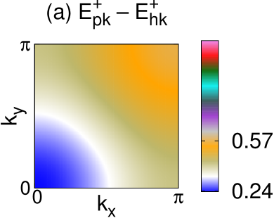
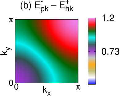
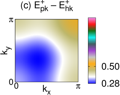
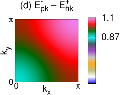
Figure 1: Density plots showing (a) intraband and (b) interband particle-hole excitation spectrum across the Brillouin zone in the Mott phase. The parameters of the system are $J=0.02U$, $\gamma=0.01U$, $\mu=0.2U$,$\Omega=0.01U$ and $\zeta=0.4$. The intraband excitations have energies between $0.24U$ to $0.57U$, while the interband excitations have energies between $0.73U$ and $1.2U$. (c) Intraband and (d) Interband particle-hole excitations in the Mott phase for $J=0.01U$, $\gamma=0.04U$, $\mu=0.2U$,$\Omega=0.01U$ and $\zeta=0.4$. In this case minimum of intraband excitations are shifted from the zone center to $(k_{0},k_{0})$ with $k_{0}=1.131a^{-1}$. The figure shows the contours in the interval $0\leq k_{x},k_{y}\leq\pi$; the contours in the other quadrants can be obtained by the reflection of the present figure around $k_{x}$ and $k_{y}$ axes and the origin. The intraband excitations have energies between $0.28U$ to $0.5U$, while the interband excitations have energies between $0.87U$ and $1.1U$. Note that the color scheme has same absolute value in all the panels to show which excitations overlap with each other in energy.

II Lattice Modulation Spectroscopy with Non-abelian gauge fields

In a system with multiple species of bosons, Raman lasers can be used to generate non-abelian gauge fields which couple the different species of bosons. In most experimental situations, the different boson species are actually different hyperfine state of the same bosonic species allowing one to treat them as a system of multi-component bosons. In fact, if one can trap two bosonic states it can be considered as an effective pseudo-spin $1/2$ system, which is however made of bosonic atoms. A particularly interesting non-abelian gauge field configuration is the Rashba spin-orbit coupling in the two component bosonic system. There are various proposals to implement the Rashba spin-orbit coupling, although currently experiments have focussed on the more easily implementable configuration of equal Rashba and Dresselhouse coupling, which leads to spins coupling to momenta in a particular direction. Interacting bosons with Rashba spin-orbit coupling shows interesting chiral Mott and superfluid phases as various parameters are tuned in the Hamiltonian xu1 ; conjun .

The Hamiltonian for two-species bosons in a square optical lattice in the presence of Rashba spin-orbit coupling term can be written as issacson ; demler1 ; haldane1

$$H_{0} = \sum_{i\sigma}[(-\Omega\sigma^{z}-\mu)n_{i\sigma}+\frac{U}{2}n_{i\sigma}(n_{i\sigma}-1)]+\zeta Un_{i\sigma}n_{i\bar{\sigma}}$$ (1)

$$-J\sum_{\langle ij\rangle\sigma}b_{i\sigma}^{\dagger}b_{j\sigma}+i\gamma\sum_{\langle ij\rangle}{\hat{\Psi}}_{i}^{\dagger}{\hat{z}}\cdot\left({\vec{\sigma}}\times{\vec{d}}_{ij}\right){\hat{\Psi}}_{j}$$

Here $b_{i\sigma}$ annihilates a boson of spin $\sigma=\uparrow,\downarrow$ on the ${\rm i^{th}}$ site, $n_{i\sigma}=b_{i\sigma}^{\dagger}b_{i\sigma}$ is the number of $\sigma$ bosons, $U(\zeta U)$ is the intra-(inter-)species interaction strength between the bosons, and $J$ denotes the nearest neighbor hopping amplitude. Here $\mu$ and $\Omega$ are the species independent and the species dependent chemical potentials; the latter acts as an effective Zeeman magnetic field for these bosons. The last term represents the lattice analogue of the Rashba spin-orbit coupling generated by the Raman lasers haldane1 ; ftnote2 , with a coupling constant $\gamma$. Here, ${\vec{d}}_{ij}$ is unit vector along the $x-y$ plane between the neighboring sites $i$ and $j$, $\vec{\sigma}$ is the vector of Pauli matrices, and $\hat{\Psi}_{i}=(b_{i\uparrow},b_{i\downarrow})$ is the two-component boson field.

The non-interacting part of the Hamiltonian is given by

$$H_{K} = \sum_{k}\Psi^{\dagger}_{k}[\hat{\Lambda}(k)-\Omega\sigma^{z}-\mu]\Psi_{k}$$

$$\hat{\Lambda}(k) = \epsilon_{k}1+\gamma_{k}\sigma^{+}+\gamma^{\ast}_{k}\sigma^{-}$$ (2)

where $k\equiv{\bf k}=(k_{x},k_{y})$ is the 2D quasi-momentum, $\epsilon_{k}=-2J(\cos k_{x}+\cos k_{y})$ and $\gamma_{k}=-2\gamma i(\sin k_{x}-i\sin k_{y})$. This can be diagonalized to obtain chiral bands touching each other at the zone center for $\Omega=0$, while a finite $\Omega$ opens up a gap between the two bands. The ratio $\gamma/J$ controls the bare dispersion including the location of the band-minima. As $\gamma/J$ becomes larger the location of the minimum of the lowest band shifts away from the zone center, $[0,0]$.

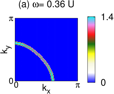
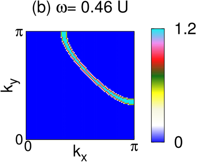
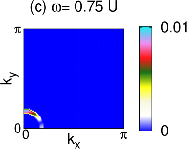
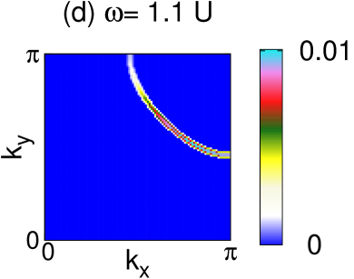
Figure 2: Lattice Modulation response in the Mott phase for different modulation frequencies. The parameters of the system are $J=0.02U$, $\gamma=0.01U$, $\mu=0.2U$,$\Omega=0.01U$ and $\zeta=0.4$. As the frequency of modulation crosses the Mott gap, a contour of intraband excitations are seen to disperse across the Brillouin zone ( a and b). Then, as the frequency crosses the interband threshold, another contour of interband excitations disperse across the Brillouin zone (c and d). Note that the spectral weight of the interband transitions are much smaller than the weights of other transitions.

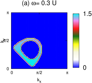
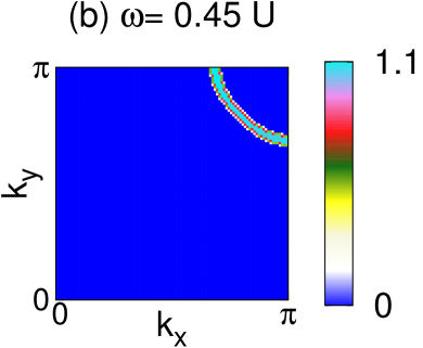
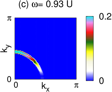
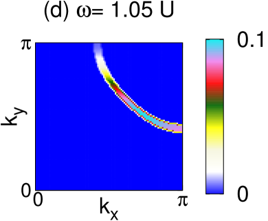
Figure 3: Lattice Modulation response in the Mott phase for different modulation frequencies. The parameters of the system are $J=0.01U$, $\gamma=0.04U$, $\mu=0.2U$,$\Omega=0.01U$ and $\zeta=0.4$. In this case minimum of intraband excitations are shifted from the zone center to $(\pm k_{0},\pm k_{0})$ with $k_{0}=1.131a^{-1}$. The figure shows the contours in the interval $0\leq k_{x},k_{y}\leq\pi$; the contours in the other quadrants can be obtained by the reflection of the present figure around $k_{x}$ and $k_{y}$ axes and the origin. As the frequency of modulation crosses the Mott gap, a contour of intraband excitations are seen to disperse across the Brillouin zone starting from a circle around $[k_{0},k_{0}]$ ( a and b). Then, as the frequency crosses the interband threshold, another contour of interband excitations disperse across the Brillouin zone starting from the zone center (c and d).

The spin-orbit coupled bosons undergo a Mott insulator to superfluid quantum phase transition as a function of $J/U$ and $\gamma/U$mandal ; grass2011 . In the strongly interacting limit, each site has exactly $n^{0}_{\sigma}$ bosons of spin $\sigma$, with the value of $n^{0}_{\sigma}$ decided by $\mu$ and $\Omega$. The system is thus a Mott insulator with no number or spin fluctuations. As $J/U$ or $\gamma/U$ increases, the system undergoes a phase transition to a state with delocalized bosons. This is the superfluid state with phase coherent Bose condensate and gapless Goldstone excitations due to broken $U(1)$ symmetry. If the transition takes place when $\gamma/J$ is large, the minimum of the effective dispersion occurs at $[\pm k_{0},\pm k_{0}]$, and the bosons condense into these finite momentum states, leading to a twisted superfluid phase mandal . At low values of $\gamma/J$ one recovers the standard superfluid with a condensate at zero momentum. Thus this system shows two remarkable qualitative changes : (a) a superfluid-Mott insulator transition as a function of $J/U$ and $\gamma/U$ and (b) a change from a standard superfluid to a twisted superfluid as a function of $\gamma/J$. As we will show, lattice modulation spectroscopy can distinguish both these phenomena and hence provide us with a wealth of information about this system.

The optical lattice modulation spectroscopy protocol that we propose consists of the following steps: (a) The optical lattice potential is weakly modulated with an a.c. field on top of the static field that forms the lattice in the original system, with the Raman fields and the trapping potential turned on. This leads to a modulation of the hopping parameter and the spin-orbit coupling. (b) The modulation is turned off after some time, making sure that the system is still in perturbative regime. At the same time, the Raman lasers, the optical lattice lasers and the trapping potential is also turned off and the system undergoes ballistic expansion, from which the (spin-resolved) momentum distribution of the system right after the modulation can be measured. (c) The change in the momentum distribution (from the unperturbed/ unmodulated system) will provide us with information about the spectrum and spectral weight of one particle excitations in these systems sensarma1 .

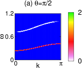
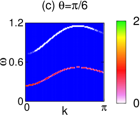
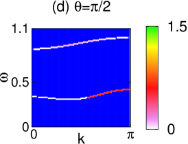
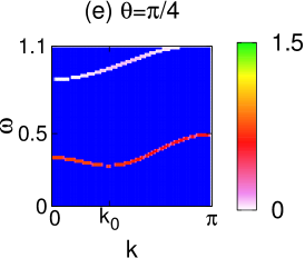
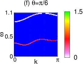
Figure 4: Lattice modulation response in the Mott phase with the variation in frequency for various cuts in the Brillouin zone going radially outwards at an angle $\theta$ with the $k_{x}$ axis. In (a) - (c) the parameters of the system are $J=0.02U$, $\gamma=0.01U$, $\mu=0.2U$,$\Omega=0.01U$ and $\zeta=0.4$ with the band minimum at the zone center. (a) $\theta=\pi/2$, (b) $\theta=\pi/4$ and (c) $\theta=\pi/6$. In (d) - (f) the parameters of the system are $J=0.01U$, $\gamma=0.04U$, $\mu=0.2U$,$\Omega=0.01U$ and $\zeta=0.4$. In this case minimum of intraband excitations are shifted from the zone center to $(k_{0},k_{0})$ with $k_{0}=1.131a^{-1}$. (d) $\theta=\pi/2$, (e) $\theta=\pi/4$ and (f) $\theta=\pi/6$.

In experiments, the lattice Hamiltonian Eq. 1 is implemented by putting a system of bosons, characterized by mass $m$, a continuum spin-orbit coupling $\gamma_{c}$ and an effective magnetic field $h$ generated by the Raman lasers, under a periodic optical potential $V_{0}[\cos^{2}(x/a)+\cos^{2}(y/a)]$, where $a=\lambda_{op}/(2\pi)$ is a transverse confinement scale used to construct the 2D square lattice, and $\lambda_{op}$ is the wavelength of the laser forming the optical lattice. The interaction between these bosons in continuum are characterized by a intra-species scattering length $a_{s}$ and an inter-species scattering length $\zeta a_{s}$. In the limit of a deep lattice, the continuum parameters are related to the lattice parameters by

$$U = 4\sqrt{V_{0}E_{R}}a_{s}/a,\quad J=\sqrt{V_{0}E_{R}}e^{-\frac{1}{4}\sqrt{V_{0}/E_{R}}}$$

$$\gamma = \gamma_{c}\frac{\sqrt{2mV_{0}}}{\hbar}e^{-\frac{1}{4}\sqrt{V_{0}/E_{R}}},$$ (3)

where $E_{R}=\hbar^{2}/2m\lambda_{op}^{2}$ is the recoil energy. It is evident that $J$ and $\gamma$ both depend exponentially on the lattice depth $V_{0}$, while $U$ has only polynomial dependence on lattice height. Thus, an ac modulation put on the optical lattice depth $V_{0}(t)=V_{0}+\delta V\cos\omega t$ will lead to simultaneous modulation of the hopping parameter, the spin orbit coupling as well as the interaction parameter $U$. Using $U$ as an overall scale for the problem, the perturbation Hamiltonian, to linear order in variations of the optical lattice potential, can be written as

$$H_{1} = \delta UH_{0}-U\delta\left(\frac{J}{U}\right)\sum_{\langle ij\rangle\sigma}b_{i\sigma}^{\dagger}b_{j\sigma}$$ (4)

$$+iU\delta\left(\frac{\gamma}{U}\right)\sum_{\langle ij\rangle}{\hat{\Psi}}_{i}^{\dagger}{\hat{z}}\cdot\left({\vec{\sigma}}\times{\vec{d}}_{ij}\right){\hat{\Psi}}_{j}$$

where the first term, proportional to the variation of $U,$ commutes with the unperturbed Hamiltonian and hence does not create excitations. This term can thus be neglected as far as modulation spectroscopy is concerned. In this case, the perturbation consists of modulating the hopping and spin-orbit terms with amplitudes ftnote1

$$\lambda = \delta J/J=\delta\gamma/\gamma=\frac{1}{8}(\delta V/\sqrt{V_{0}E_{R}})$$ (5)

The perturbation Hamiltonian can then be written as

$$H_{1}(t)=\lambda\cos\omega t\sum_{k}\Psi^{\dagger}_{k}\hat{\Lambda}(k)\Psi_{k}.$$ (6)

In linear response regime, the momentum distribution right after the modulation is turned off oscillates with the frequency of the perturbation sensarma1

$$\delta n_{\sigma,k}(t)=\delta n^{(1)}(\sigma,k,\omega)\cos\omega t+\delta n^{(2)}(\sigma,k,\omega)\sin\omega t$$ (7)

The out-of phase response contains the information about excitation spectrum of the unperturbed system. In the next section, we will define the response function $\Pi_{\sigma}(k,i\omega)$, where $i\omega$ is the Matsubara frequency, and relate this to the single particle Green’s function of the bosons and hence to the excitation spectra. The imaginary part of $\Pi_{\sigma}(k,\omega+i0^{+})$ then measures the amplitude of the out of phase modulation of the spin dependent momentum distribution due to the perturbation. The structure of the response is qualitatively different in the Mott and superfluid phase owing to the broken $U(1)$ symmetry in the superfluid phase and associated anomalous propagators. Hence we will treat the response in the Mott and superfluid phase separately.

III Response in the Mott phase

In the strongly interacting limit, the system is in an incompressible Mott insulating state with gapped excitation spectrum. In the atomic limit, ($\gamma=J=0$), the ground state has a fixed number of bosons of each spin, $n^{0}_{\sigma}$ at all the sites. In general, $n^{0}_{\sigma}$ is determined by the values of $\mu$ and $\Omega$. We will restrict our analysis to the case where $n^{0}_{\uparrow}=1$ and $n^{0}_{\downarrow}=0$, but the analysis can be easily extended to arbitrary integer values of $n^{0}_{\sigma}$. The single particle Green’s function in the Mott phase is a $2\times 2$ matrix in the spin space, in terms of which the response function is given by

$$\Pi_{\sigma}(k,i\omega_{n}) = \frac{\lambda}{\beta}\sum_{\omega_{l}}[\hat{G}(k,i\omega_{l})\hat{\Lambda}(k)\hat{G}(k,i\omega_{l}+i\omega_{n})]_{\sigma\sigma}$$ (8)

$$+(\omega_{n}\rightarrow-\omega_{n})$$

The boson Green’s function can be worked out in a strong coupling expansion around the localized atomic limit sengupta1 ; mandal ; grass2011 . In the Mott phase, it is given by

$$G^{-1}(k,i\omega_{n}) = \left(\begin{array}[]{cc}F_{1}(i\omega_{n})-\epsilon_{k}&-\gamma_{k}\\ -\gamma^{\ast}_{k}&F_{2}(i\omega_{n})-\epsilon_{k}\end{array}\right)$$ (11)

$$F_{1}(i\omega_{n}) = i\omega_{n}+E_{0}-2U+2U^{2}/(i\omega_{n}+E_{0}+U),$$

$$F_{2}(i\omega_{n}) = i\omega_{n}-E_{1}$$ (12)

where $E_{0}=\mu+\Omega$ and $E_{1}=\Omega+\zeta U-\mu$.

It is evident that this Green’s function is not diagonal in the basis of non-interacting bands, as the atomic limit local propagator is different for the 2 spin species. This can be traced to the fact that in the atomic limit ($J=0$, $\gamma=0$) the $\Omega$ term lifts the degeneracy between the spin states and as a result one obtains a polarized Mott state which is $n_{0}=1$ for the $\uparrow$ spins and $n_{0}=0$ (vacuum) for the $\downarrow$ spins. The Green’s function can, however, be diagonalized to obtain

$$G_{D}(k,i\omega_{n})=\left(\begin{array}[]{cc}\frac{1}{\zeta_{-}(k,i\omega_{n})}&0\\ 0&\frac{1}{\zeta_{+}(k,i\omega_{n})}\end{array}\right)$$ (13)

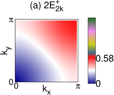
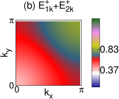
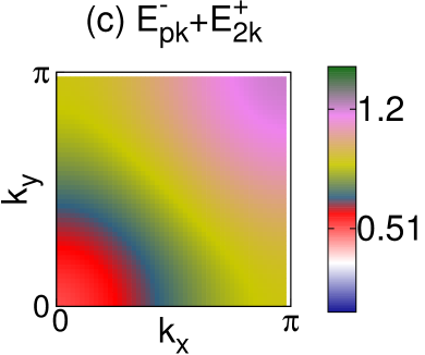
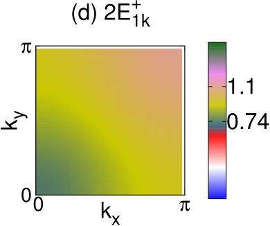
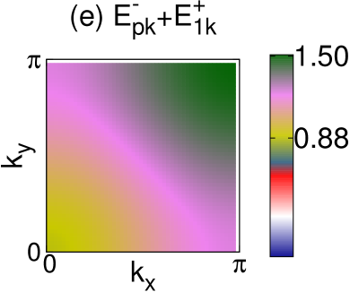
Figure 5: Excitation spectrum in the superfluid phase. The parameters of the system are $J=0.03U$, $\gamma=0.01U$, $\mu=0.35U$, $\Omega=0.01U$ and $\zeta=0.4$. In this case the BEC is formed at the zone center. The excitations are (a) two phase modes (b) one phase and one amplitude mode (c) one phase mode and one interband transition (d) two amplitude modes and (e) an amplitude mode and an interband transition. Note that the color scheme has same absolute value in all panels to show which excitations overlap with each other in energy.

where the diagonal components are given by

$$\zeta_{\pm}(k,i\omega_{n})=F_{+}(i\omega_{n})-\epsilon_{k}\pm(F^{2}_{-}(i\omega_{n})+|\gamma_{k}|^{2})^{1/2},$$ (14)

and $F_{\pm}(i\omega_{n})=(1/2)[F_{1}(i\omega_{n})\pm F_{2}(i\omega_{n})]$. The basis transform, which diagonalizes the Green’s function is given by

$$M(k,i\omega_{n}) = \left(\begin{array}[]{cc}u(k,i\omega_{n})&v(k,i\omega_{n})\\ -v^{\ast}(k,i\omega_{n})&u^{\ast}(k,i\omega_{n})\end{array}\right)$$ (17)

$$|u(k,i\omega_{n})|^{2} = \gamma_{k}^{2}/N(k,i\omega_{n})$$

$$v(k,i\omega_{n}) = \gamma_{k}^{-1}u^{\ast}(k,i\omega_{n})[F_{1}(i\omega_{n})-\epsilon_{k}-\zeta_{+}(k,i\omega_{n})],$$

$$N(k,i\omega_{n}) = \sqrt{[F_{1}(i\omega_{n})-\epsilon_{k}-\zeta_{+}(k,i\omega_{n})]^{2}+\gamma_{k}^{2}}.$$ (18)

Note that $|u(k,i\omega_{n})|^{2}+|v(k,i\omega_{n})|^{2}=1$.

It is evident from the above expressions that even in the transformed basis, the diagonal Green’s function (Eq.  13) will have a complicated frequency dependence. However, we are only interested in the out of phase response of the system to the external perturbation, which depends solely on the imaginary part of the Green’s function, analytically continued to the real frequency domain ($i\omega_{n}\rightarrow\omega+i0^{+}$). It can be easily shown that the retarded Green’s function only has simple poles, and so, for the purpose of calculating the out of phase response, the complicated expression of Eq. 13 can be replaced by the simpler form

$$G_{D}(k,i\omega_{n})\simeq\left(\begin{array}[]{cc}\frac{z^{-}_{pk}}{i\omega_{n}-E^{-}_{pk}}&0\\ 0&\frac{z^{+}_{pk}}{i\omega_{n}-E^{+}_{pk}}+\frac{z^{+}_{hk}}{i\omega_{n}-E^{+}_{hk}}\end{array}\right)$$ (19)

where $\omega=E^{+}_{p(h)k}$ are the two zeroes of $\zeta^{+}(k,\omega)$ and correspond to the particle and hole excitations of the $+$ band, while $\omega=E^{-}_{pk}$ is the zero of $\zeta^{-}(k,\omega)$. The residues $z$ are given by the $\omega$ derivative of the components of the Green’s function, Eq. 13, evaluated at the corresponding poles. The three poles have a relatively simple explanation in terms of the particle and hole excitations of a Mott insulator. In absence of the spin-orbit coupling ($\gamma=0$), the $\uparrow$ spins form a $n_{0}=1$ Mott insulator and has the corresponding particle and hole excitations. This corresponds to the limiting form of $E^{+}_{p(h)k}$ as $\gamma\rightarrow 0$. The $\downarrow$ spins , however, form a $n_{0}=0$ Mott insulator, and hence has only particle excitations. This is the limiting form of $E^{-}_{pk}$ in the limit $\gamma\rightarrow 0$. In presence of spin-orbit coupling, the spin states get mixed, but this three pole structure of the Green’s function persists. We note that the Green’s function in Eq. 19 has the same imaginary part as the actual Green’s function (Eq.  13) and hence there is no approximation made in the above replacement, as far as computation of the out of phase response of the system is concerned.

The response of the system can now be calculated in terms of the diagonal Green’s function as

$$\Pi_{\sigma}(k,i\omega_{n}) = \frac{\lambda}{\beta}\sum_{i\omega_{l}}\left[M(k,i\omega_{l})G_{D}(k,i\omega_{l})M^{-1}(k,i\omega_{l})\hat{\Lambda}(k)M(k,i\omega_{l}+i\omega_{n})G_{D}(k,i\omega_{l}+i\omega_{n})M^{-1}(k,i\omega_{l}+i\omega_{n})\right]_{\sigma\sigma}$$ (20)

$$+\omega_{n}\rightarrow-\omega_{n},$$

where ${\hat{\Lambda}}(k)$ is given by Eq. 2. Note that the transformation matrices are themselves function of the Matsubara frequencies $i\omega_{l}$ and $i\omega_{n}$. However, it can be easily seen that the transformation matrix elements, analytically continued to the real frequency domain ($i\omega_{l}\rightarrow\omega+i0^{+}$), have no imaginary part, and hence the real frequency response will be dominated by the singularities of the diagonal Green’s function only.

Analytically continuing to real frequencies and working out the Matsubara sums (and noting that matrix elements of $M$ are real in this limit), we get

$$n^{(2)}(\sigma,k,\omega)=2\lambda\sum_{pq}\int_{-\infty}^{\infty}\frac{d\omega^{\prime}}{\pi}\alpha^{\sigma}_{pq}(k,\omega^{\prime},\omega+\omega^{\prime})G_{D}^{p^{\prime\prime}}(k,\omega^{\prime})G_{D}^{q^{\prime\prime}}(k,\omega+\omega^{\prime})[n_{B}(\omega^{\prime})-n_{B}(\omega^{\prime}+\omega)]$$ (21)

where $p,q=\pm$, $G_{D}^{p^{\prime\prime}}$ indicates the imaginary part of the Green’s function component, and the matrix element

$$\alpha^{\sigma}_{pq}(k,\omega_{1},\omega_{2}) = \sum_{mn}M_{\sigma p}(k,\omega_{1})M^{-1}_{pm}(k,\omega_{1})\hat{\Lambda}_{mn}(k)M_{nq}(k,\omega_{2})M^{-1}_{q\sigma}(k,\omega_{2})$$ (22)

We now restrict ourselves to the response at $T=0$. From the simple pole structure of the Green’s function the response is then obtained as

$$n^{(2)}(\sigma,k,\omega) = 2\pi\lambda\left[\alpha^{\sigma}_{++}(k,E^{+}_{pk},E^{+}_{hk})z^{+}_{pk}z^{+}_{hk}\delta(\omega-E^{+}_{pk}+E^{+}_{hk})+\alpha^{\sigma}_{+-}(k,E^{-}_{pk},E^{+}_{hk})z^{+}_{hk}z^{-}_{pk}\delta(\omega-E^{-}_{pk}+E^{+}_{hk})\right.$$ (23)

$$\left.+\alpha^{\sigma}_{++}(k,E^{+}_{hk},E^{+}_{pk})z^{+}_{pk}z^{+}_{hk}\delta(\omega-E^{+}_{hk}+E^{+}_{pk})+\alpha^{\sigma}_{+-}(k,E^{+}_{hk},E^{-}_{pk})z^{+}_{hk}z^{-}_{pk}\delta(\omega-E^{+}_{hk}+E^{-}_{pk})\right]$$

It is clear from Eq. 23 that the response shows up on two contours specified by $\omega=E^{+}_{pk}-E^{+}_{hk}$ and $\omega=E^{-}_{pk}-E^{+}_{hk}$, the intra and interband particle-hole excitations. In the Mott phase, both these excitations are gapped with the lowest Mott gap corresponding to the intra-band excitations. As the frequency of modulation is swept, there is no response till the frequency crosses the Mott gap. Beyond this point, two distinctive set of phenomena can be seen depending on the ratio, $\gamma/J$. For small $\gamma/J$ the minimum of the intraband excitations is at the zone center, $[0,0]$. This is seen in Fig. 1(a), where the intraband excitation in the Brillouin zone is plotted as a color plot for the following set of parameters: $J=0.02U$, $\gamma=0.01U$, $\Omega=0.01U$, $\mu=0.2U$ and $\zeta=0.4$, where the minimum of the spectrum (the Mott gap) is $0.24U$ at the zone center. The dispersion increases as one moves away from the zone center and the highest excitation energy occur at $[\pi,\pi$ with $\omega=0.57U$. The corresponding inter-band excitations are shown in Fig. 1(b). They follow a similar pattern as the intra-band excitations with a minimum energy of $0.73U$ and a maximum energy of $1.22U$.

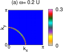
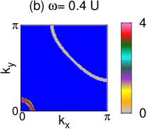
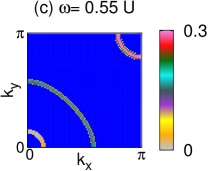
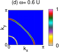
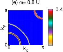
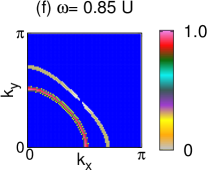
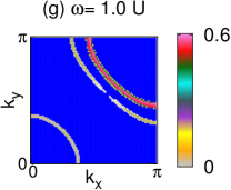
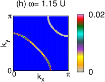
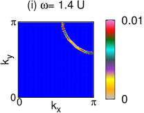
Figure 6: Lattice modulation response in the superfluid phase. The parameters of the system are $J=0.03U$, $\gamma=0.01U$, $\mu=0.35U$,$\Omega=0.01U$ and $\zeta=0.4$. In this case the BEC is formed at the zone center. (a) A single contour corresponding to the two phase modes (b) 2 contours (outward from zone center): a phase and an amplitude mode, two phase modes (c) 3 contours (outward from zone center): a phase mode and an interband transition, a phase and an amplitude mode, two phase modes (d) 2 contours (outward from zone center): a phase mode and an interband transition, a phase and an amplitude mode (e) 3 contours (outward from zone center): two amplitude modes, a phase mode and an interband transition, a phase and an amplitude mode (f) 2 contours (outward from zone center): two amplitude modes, a phase mode and an interband transition (g) 3 contours (outward from zone center): an amplitude mode and an interband transition, two amplitude modes, a phase and an interband transition (h) 2 contours (outward from zone center): an amplitude mode and an interband transition, two amplitude modes (i) a single contour: an amplitude mode and an interband transition. Note that the spectral weight of the interband transitions are much smaller than the weights of other transitions.

The optical modulation response in this case is plotted for four different frequencies in this case in Fig. 2. As frequency increases beyond the gap, $0.24U$, a contour of excitations is seen, which become larger and moves towards the edge of the Brillouin zone, before disappearing at $\omega=0.57U$. This contour, corresponding to intra-band excitations, are shown in Fig 2(a) and (b). As the frequency is further increased beyond $\omega=0.73U$, the contours corresponding to the inter-band excitations appear around the zone center and move outwards, before disappearing at $\omega=1.22U$, as shown in Fig 2(c) and (d). We would like to note here that the full dispersion of the excitations can be tracked from the optical lattice modulation spectroscopy. To show how this is done, in Fig. 4 we plot the lattice modulation response in the Mott phase as a function of frequency along various cuts in the Brillouin zone, going radially outwards at different angles $\theta$ with the $k_{x}$ axis. Fig.  reffig8 (a)-(c) correspond to the system parameters $J=0.02U$, $\gamma=0.01U$, $\mu=0.2U$,$\Omega=0.01U$ and $\zeta=0.4$ with the band minimum at the zone center, which is clearly seen from the plots. Further, the modulation spectroscopy also provide information about the spectral weight of the various excitations. In this case, it is evident the interband excitations carry much less spectral weight than the intraband excitations.

The phenomenology changes dramatically if the spin orbit coupling $\gamma$ is larger than hopping $J$. Fig. 1(c) and (d) shows a plot of the intra and interband particle hole excitations in the Mott phase for a system with parameter values $J=0.01U$, $\gamma=0.04U$, $\Omega=0.01U$, $\mu=0.2U$ and $\zeta=0.4$. In this case the spin orbit coupling is larger than the hopping and consequently the intraband excitations have a minimum at $[\pm k_{0},\pm k_{0}]$ along the zone diagonal. The location of the minima corresponding $[k_{0},k_{0}]$ is shown in Fig. 1(c); the corresponding figures for other minima can be obtained by a reflection of the contours in the first quadrant ($0\leq k_{x},k_{y}\leq\pi)$ about the $k_{x}$ and $k_{y}$ axes and the origin. The interband excitations however have a minimum at the zone center, as seen in Fig. 1(d). Once again, the system will not show any response as long as the modulation frequency is below the Mott gap of $0.28U$. Once the Mott gap is crossed, excitation contours around $[\pm k_{0},\pm k_{0}]$ appear in the response, as seen (for $[k_{0},k_{0}]$) in Fig 3(a). These contours spread out and disappear at $\omega=0.45U$, as seen in Fig 3(b). Another contour, corresponding to interband excitations and centered around $k=0$ appears as the modulation frequency is swept beyond $0.87U$. This spreads out and finally disappears at $\omega=1.1U$, the upper limit of the interband excitation energy, as seen in Fig. 3(c) and (d). To get a better idea of the dispersion, the lattice modulation response for a system in Mott phase with a band minimum shifted to finite wavevectors is plotted in Fig.  4 (d) - (f), where the parameters of the system are $J=0.01U$, $\gamma=0.04U$, $\mu=0.2U$,$\Omega=0.01U$ and $\zeta=0.4$. In this case, the band minimum is at $(k_{0},k_{0})$ with $k_{0}=1.131a^{-1}$. It is clearly seen that the intraband excitations have a shifted band minimum, while the interband excitations continue to have a minima at the zone center. In this case, it is clear from comparison with corresponding response in Fig. 2, that although the intraband excitations have larger spectral weight than the interband excitations, the interband excitations carry relatively larger spectral weight than the case where the minimum was at the zone center.

The lattice modulation spectroscopy can identify the Mott phase from the existence of a gap in the spectrum. However the momentum resolved nature of the spectroscopy provides much more detailed information about the single particle spectral function of the system. It provides information about the spectrum and one should be clearly able to see the minimum of the excitation spectrum shift from the zone center as the parameters are varied. The modulation spectroscopy also provides information about the spectral weight of the excitations of the system, which is of immediate relevance for figuring out both near equilibrium and far from equilibrium response of the system to different stimuli.

IV Response in the Superfluid phase

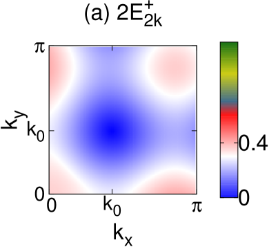
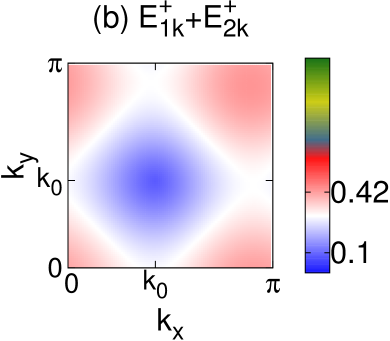
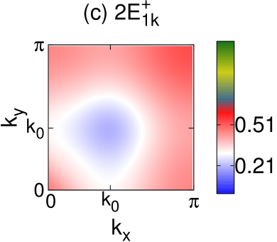
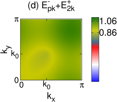
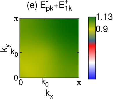
Figure 7: Excitation spectrum in the superfluid phase. The parameters of the system are $J=0.01U$, $\gamma=0.06U$, $\mu=0.2U$,$\Omega=0.01U$ and $\zeta=0.4$. In this case the BEC is formed at a finite momentum $[\pm k_{0},\pm k_{0}]$, with $k_{0}=1.34a^{-1}$, away from the zone center. The excitations are (a) two phase modes (b) one phase and one amplitude mode (c) one phase mode and one interband transition (d) two amplitude modes and (e) an amplitude mode and an interband transition. Note that the color scheme has same absolute value in all panels to show which excitations overlap with each other in energy.

The spin-orbit coupled bosons undergo a Mott insulator-superfluid quantum phase transition as either the hopping or the spin-orbit coupling is increased as both terms help to delocalize the bosons. If the transition occurs at a large value of $J/\gamma$, the superfluid phase has a BEC at the zone center $k=[0,0]$ with associated anomalous propagators and Goldstone modes. On the other hand, if the transition takes place at a large value of $\gamma/J$, the system exhibits the twisted superfluid phase, with a BEC at a finite momentum. In general there can be four such momentum values given by $[\pm k_{0},\pm k_{0}]$ which are degenerate minima of the spectrum. This in principle allows the possibility of formation of a square superlattice (i.e. a supersolid) with the incommensurate momentum $k_{0}$ providing the inverse lattice constant. However, in a cold atom system with the presence of a trapping potential which breaks translational symmetry, the more likely effect is the formation of domains powell , each of which corresponds to choosing one of the four values of allowed $k_{0}$. Assuming domains of size much larger than $k_{0}^{-1}$, the momentum distribution signal will be an incoherent weighted sum of the signal from a single domain with a fixed condensation wavevector. In this paper, we shall assume that condensation occurs at only one possible momentum which we choose to be $(k_{0},k_{0})$ and work out the signal from a single domain. The important features, like the low energy features around$(k_{0},k_{0})$ will occur in different parts of the Brillouin zone for different domains and thus will not be washed out by formation of domains. Although the detailed signal requires knowledge of domain distribution, a first approximation can be obtained from our calculation by symmetry, together with an idea of the density of each type of domains. The lattice modulation spectroscopy is uniquely suited to distinguish between gapless superfluid phase from the Mott phase, and owing to its momentum resolved nature, it can also distinguish between the normal and twisted superfluid phases. Since this method gives detailed information about the spectral function, useful quantities like the speed of sound can be calculated from the spectrum, while the relative intensity of the contours will provide information about transfer of spectral weight among the different kinds of excitations as the energy is varied.

In the superfluid phase the bosons occupying the lower energy band form a BEC at the appropriate momentum. In this case the Green’s functions expand to a $4\times 4$ matrix to accommodate the anomalous propagators. It is easier to work in the $\pm$ basis, earlier described in the Mott phase, since the structure of the Green’s functions are simplest in this basis. Working with a $4$ component vector $[\phi^{-}(k,i\omega),\phi^{-\ast}(2k_{0}-k,-i\omega),\phi^{+}(k,i\omega),\phi^{+\ast}(2k_{0}-k,-i\omega)]$, the inverse Green’s function is given by mandal ; sensarma1 ; sengupta1

$$G^{-1}(k,i\omega_{n})\simeq\left(\begin{array}[]{cccc}\zeta_{-}(k,i\omega_{n})-r&0&0&0\\ 0&\zeta_{-}(2k_{0}-k,-i\omega_{n})-r&0&0\\ 0&0&\zeta_{+}(k,i\omega_{n})-r&-r\\ 0&0&-r&\zeta_{+}(2k_{0}-k,-i\omega_{n})-r\\ \end{array}\right)$$ (24)

where $\zeta_{\pm}(k,i\omega)$ is defined by Eq. 14 and $r=\zeta_{+}(k_{0},k_{0},\omega=0)$ incorporates the effects of the presence of the condensate. The lower $2\times 2$ block simply looks like the Green’s function of a Bose gas in the Bogoliubov approximation, with the complicated function $\zeta_{+}(k,\omega)$, incorporating correlations due to proximity to a Mott insulator, replacing a simple free particle piece. In the diagonal upper block, the presence of the condensate leads to a Hartree correction due to inter-band interactions.

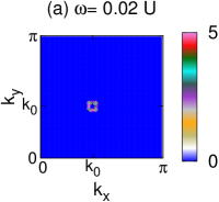
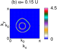
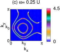
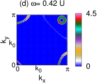
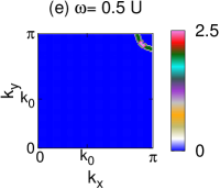
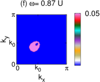
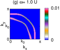
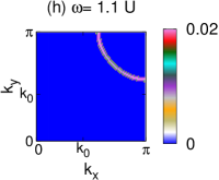
Figure 8: Lattice modulation response in the superfluid phase. The parameters of the system are $J=0.01U$, $\gamma=0.06U$, $\mu=0.2U$,$\Omega=0.01U$ and $\zeta=0.4$. In this case the BEC is formed at a finite momentum $[k_{0},k_{0}]$ ($k_{0}=1.34a^{-1}$) away from the zone center. A single contour corresponding to the two phase modes (b) 2 contours (outward from zone center): a phase and an amplitude mode, two phase modes (c) 4 contours : two open contours due to two phase modes, and two closed contours (outward from the zone center) due to two amplitude modes, a phase and an amplitude mode (d) closed contour due to a phase and an amplitude mode and open contours due to two amplitude modes, (e) a single contour: two amplitude modes (f) a single contour: a phase mode and an interband transition at finite momentum (g) 2 contours (outward from zone center): an amplitude mode and an interband transition, a phase and an interband transition (h) a single contour: an amplitude mode and an interband transition. Note that the spectral weight of the interband transitions are much smaller than the weights of other transitions.

The unitary transform which converts the original “spin” basis, i.e. $[\phi_{\uparrow}(k,i\omega),\phi^{\ast}_{\uparrow}(2k_{0}-k,-i\omega),\phi_{\downarrow}(k,i\omega),\phi^{\ast}_{\downarrow}(2k_{0}-k,-i\omega)]$, to the $\pm$ basis is given by

$$\tilde{M}(k,i\omega_{n})\simeq\left(\begin{array}[]{cccc}M_{11}^{\ast}(k,i\omega)&0&M_{21}^{\ast}(k,i\omega)&0\\ 0&M_{11}(2k_{0}-k,-i\omega)&0&M_{21}(2k_{0}-k,-i\omega)\\ M_{12}^{\ast}(k,i\omega)&0&M_{22}^{\ast}(k,i\omega)&0\\ 0&M_{12}(2k_{0}-k,-i\omega)&0&M_{22}(2k_{0}-k,-i\omega)\end{array}\right),$$ (25)

where the matrix elements $M_{ij}$ are given by Eq. 18. The final Green’s function has the form

$$G(k,i\omega_{n})=\left(\begin{array}[]{cccc}G^{-}(k,i\omega_{n})&0&0&0\\ 0&G^{-}(2k_{0}-k,-i\omega_{n})&0&0\\ 0&0&G^{+}(k,i\omega_{n};k_{0})&F(k,i\omega_{n};k_{0})\\ 0&0&F(2k_{0}-k,-i\omega_{n};k_{0})&G^{+}(2k_{0}-k,-i\omega_{n};k_{0})\\ \end{array}\right).$$ (26)

The full expression for the Green’s functions are complicated, but, as in the case of the Mott phase, the only singularities of the Green’s functions are simple poles. So, as far as the imaginary part of the Green’s function is concerned, they are faithfully reproduced by

$$G^{-}(k,i\omega) = \frac{g^{-}_{pk}}{i\omega-E^{-}_{pk}},\quad G^{+}(k,i\omega;k_{0})=\frac{g^{+p}_{1k}}{i\omega-E^{+}_{1k}}+\frac{g^{+h}_{1k}}{i\omega+E^{+}_{1k}}+\frac{g^{+p}_{2k}}{i\omega-E^{+}_{2k}}+\frac{g^{+h}_{2k}}{i\omega+E^{+}_{2k}}$$ (27)

$$F(k,i\omega;k_{0}) = \frac{f^{+}_{1k}}{i\omega-E^{+}_{1k}}-\frac{f^{+}_{1k}}{i\omega+E^{+}_{1k}}+\frac{f^{+}_{2k}}{i\omega-E^{+}_{2k}}-\frac{f^{+}_{2k}}{i\omega+E^{+}_{2k}}$$ (28)

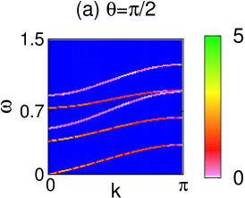
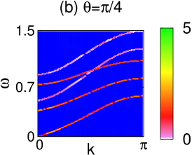
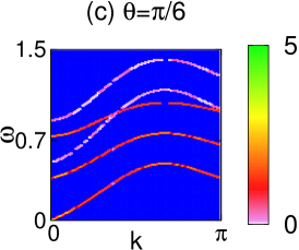
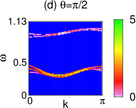
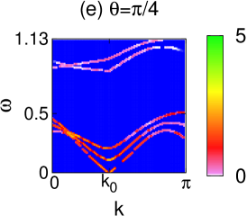
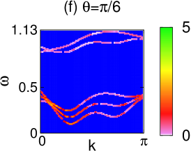
Figure 9: Lattice modulation response in the superfluid phase with the variation in frequency for various cuts in the Brillouin zone going radially outwards at an angle $\theta$ with the $k_{x}$ axis. In (a) - (c) the parameters of the system are $J=0.03U$, $\gamma=0.01U$, $\mu=0.35U$,$\Omega=0.01U$ and $\zeta=0.4$ with the condensate at the zone center. (a) $\theta=\pi/2$, (b) $\theta=\pi/4$ and (c) $\theta=\pi/6$. All the five branches including the gapless linear Goldstone mode near $k=0$ is clearly seen. In (d) - (f) the parameters of the system are $J=0.01U$, $\gamma=0.06U$, $\mu=0.2U$,$\Omega=0.01U$ and $\zeta=0.4$. In this case the condensate is located at $(k_{0},k_{0})$ with $k_{0}=1.131a^{-1}$. (d) $\theta=\pi/2$, (e) $\theta=\pi/4$ and (f) $\theta=\pi/6$. Only the cut along $[1,1]$ direction passes through the condensate location and shows the gapless Goldstone mode, while the spectrum is gapped along the other cuts.

Here the particle excitation in the $-$ branch, $E^{-}_{pk}$ is the solution of $\zeta_{-}(k,E^{-}_{pk})=r$ and the four excitation poles $\pm E^{+}_{1(2)k}$ are obtained from the solutions of

$$[\zeta_{+}(k,\omega)-2r][\zeta_{+}(2k_{0}-k,-\omega)-2r]-r^{2}=0.$$ (29)

The quasiparticle residues are obtained from the frequency derivatives of the Green’s functions at the corresponding poles. Note that in the $+$ band, the particle and hole excitations are now mixed due to formation of a condensate and that the energies $E_{1(2)k}^{+}$, $g^{+p(h)}_{1(2)k}$, and $f^{+}_{1(2)k}$ depends on $k_{0}$ through Eq. 29; this is in contrast to the corresponding quantities in the $-$ band which has no particle-hole mixing. This necessitates the use of additional $k_{0}$ argument in the definition of $G^{+}$ and $F$ in Eq. 26; however, we refrain from putting such additional label of $k_{0}$ in $E_{1(2)k}^{+}$, $g^{+p(h)}_{1(2)k}$, and $f^{+}_{1(2)k}$ for notational brevity.

The response function for the lattice modulation spectroscopy is then given by

$$\Pi_{\sigma}(k,i\omega_{n}) = \frac{\lambda}{\beta}\sum_{i\omega_{l}}\left[\tilde{M}(k,i\omega_{l})G(k,i\omega_{l})\tilde{M}^{-1}(k,i\omega_{l})\hat{\Lambda}^{{}^{\prime}}(k)\tilde{M}(k,i\omega_{l}+i\omega_{n})G(k,i\omega_{l}+i\omega_{n})\tilde{M}^{-1}(k,i\omega_{l}+i\omega_{n})\right]_{2a-1,2a-1}$$ (30)

$$+\omega_{n}\rightarrow-\omega_{n}$$

where $a=1$ for $\sigma=\uparrow$ and $a=2$ for $\sigma=\downarrow$, and the perturbation matrix $\Lambda^{\prime}$ is given by

$$\Lambda^{{}^{\prime}}(k)=\frac{1}{2}\left(\begin{array}[]{cccc}\epsilon_{k}&0&\gamma_{k}&0\\ 0&\epsilon_{k}&0&\gamma^{\ast}_{-k}\\ \gamma^{\ast}_{k}&0&\epsilon_{k}&0\\ 0&\gamma_{-k}&0&\epsilon_{k}\end{array}\right)$$ (31)

Working out the Matsubara sums, and analytically continuing to real frequencies,

$$n^{(2)}(\sigma,k,\omega) = 2\lambda\left[\sum_{pq}\int_{-\infty}^{\infty}\frac{d\omega^{\prime}}{\pi}\alpha^{\sigma}_{pq}(k,\omega^{\prime},\omega+\omega^{\prime})G^{p^{\prime\prime}}(k,\omega^{\prime};k_{0})G^{q^{\prime\prime}}(k,\omega+\omega^{\prime};k_{0})[n_{B}(\omega^{\prime})-n_{B}(\omega^{\prime}+\omega)]\right.$$ (32)

$$\left.+\beta^{\sigma}(k,\omega^{\prime},\omega+\omega^{\prime})F^{{}^{\prime\prime}}(k,\omega^{\prime};k_{0})F^{{}^{\prime\prime}}(k,\omega-\omega^{\prime};k_{0})[n_{B}(\omega^{\prime})-n_{B}(\omega-\omega^{\prime})\right]$$

where $p,q=\pm$, $G^{p^{\prime\prime}}$ and $F^{{}^{\prime\prime}}$ indicate the imaginary part of the Green’s function component, and it is understood that $G^{-^{\prime\prime}}(k,\omega;k_{0})\equiv G^{-^{\prime\prime}}(k,\omega)$. Here the matrix elements

$$\alpha^{\sigma}_{pq}(k,\omega_{1},\omega_{2}) = \sum_{mn}\tilde{M}_{2\sigma-1p}(k,\omega_{1})\tilde{M}^{-1}_{pm}(k,\omega_{1})\hat{\Lambda}^{{}^{\prime}}_{mn}(k)\tilde{M}_{nq}(k,\omega_{2})\tilde{M}^{-1}_{q2\sigma-1}(k,\omega_{2})$$

$$\beta^{\sigma}(k,\omega_{1},\omega_{2}) = \sum_{mn}\tilde{M}_{2\sigma-1,3}(k,\omega_{1})\tilde{M}^{-1}_{2m,4}(k,\omega_{1})\hat{\Lambda}^{{}^{\prime}}_{2n,2m}(k)\tilde{M}_{2n,4}(k,\omega_{2})\tilde{M}^{-1}_{2\sigma-1,3}(k,\omega_{2})$$ (33)

We now restrict ourselves to the response at $T=0$ for $\omega>0$. The $\omega<0$ response can then be obtained from the fact that the imaginary part of the response function is an odd function of $\omega$. From the simple pole structure of the Green’s function the response is then obtained as

$$n^{(2)}(\sigma,k,\omega) = 2\pi\lambda\left[\rho^{\sigma}_{1}(k)\delta(\omega-E^{-}_{pk}-E^{+}_{1k})+\rho^{\sigma}_{2}(k)\delta(\omega-E^{-}_{pk}-E^{+}_{2k})\right.$$ (34)

$$\left.\rho^{\sigma}_{3}(k)\delta(\omega-2E^{+}_{1k})+\rho^{\sigma}_{4}(k)\delta(\omega-2E^{+}_{2k})+\rho^{\sigma}_{5}(k)\delta(\omega-E^{+}_{1k}-E^{+}_{2k})\right]$$

where the weight of the different contours are given by

$$\rho^{\sigma}_{1}(k) = 2g^{-}_{pk}g^{+h}_{1k}\alpha^{\sigma}_{12}(k,E^{-}_{pk},-E^{+}_{1k})~{}~{}~{}~{}~{}~{}~{}~{}~{}~{}~{}~{}~{}~{}~{}~{}~{}~{}~{}\rho^{\sigma}_{2}(k)=2g^{-}_{pk}g^{+h}_{2k}\alpha^{\sigma}_{12}(k,E^{-}_{pk},-E^{+}_{2k})$$

$$\rho^{\sigma}_{3}(k) = 2g^{+p}_{1k}g^{+h}_{1k}\alpha^{\sigma}_{22}(k,E^{+}_{1k},-E^{+}_{1k})-(f^{+}_{1k})^{2}[\beta^{\sigma}(k,E^{+}_{1k},E^{+}_{1k})+\beta^{\sigma}(k,-E^{+}_{1k},-E^{+}_{1k})]$$ (35)

$$\rho^{\sigma}_{4}(k) = 2g^{+p}_{2k}g^{+h}_{2k}\alpha^{\sigma}_{22}(k,E^{+}_{2k},-E^{+}_{2k})-(f^{+}_{2k})^{2}[\beta^{\sigma}(k,E^{+}_{2k},E^{+}_{2k})+\beta^{\sigma}(k,-E^{+}_{2k},-E^{+}_{2k})]$$

$$\rho^{\sigma}_{5}(k) = 2g^{+p}_{1k}g^{+h}_{2k}\alpha^{\sigma}_{22}(k,E^{+}_{1k},-E^{+}_{2k})+2g^{+p}_{2k}g^{+h}_{2k}\alpha^{\sigma}_{22}(k,-E^{+}_{1k},E^{+}_{2k})-2f^{+}_{1k}f^{+}_{2k}[\beta^{\sigma}(k,E^{+}_{1k},E^{+}_{2k})+\beta^{\sigma}(k,-E^{+}_{2k},-E^{+}_{1k})]$$

It is clearly seen that the system would show response on the contours which correspond to energies $2E^{+}_{1k}$, $2E^{+}_{2k}$, $E^{+}_{1k}+E^{+}_{2k}$, $E^{-}_{pk}+E^{+}_{1k}$ and $E^{-}_{pk}+E^{+}_{2k}$. Here $E^{+}_{2k}$ is the Goldstone phase mode which goes gapless, $E^{+}_{1k}$ is the gapped amplitude or Higgs mode and $E^{-}_{pk}$ is the particle excitation to the upper band, which also has an excitation gap. The location of these contours in the Brillouin zone are dramatically different depending on whether the BEC is formed at the zone center (large $J/\gamma$) or at a finite momentum (small $J/\gamma$).

The dispersions of $2E^{+}_{1k}$, $2E^{+}_{2k}$, $E^{+}_{1k}+E^{+}_{2k}$, $E^{-}_{pk}+E^{+}_{1k}$ and $E^{-}_{pk}+E^{+}_{2k}$ are plotted in Fig. 5 for a system with following set of parameters: $J=0.03U$, $\gamma=0.01U$, $\Omega=0.01U$, $\mu=0.35U$ and $\zeta=0.4$. In this case, the system is in a superfluid with a BEC at the zone center. Fig. 5 (a) shows $2E^{+}_{2k}$, which ranges from $0$ at the zone center (the gapless point) to $0.58U$. All the other plots in Fig. 5 show similar features except the fact that these excitations are gapped. In Fig. 5 (b), $E^{+}_{1k}+E^{+}_{2k}$ ranges from $0.37U$ to $0.83U$. Similarly $E^{-}_{pk}+E^{+}_{2k}$ [Fig. 5 (c)] ranges from $0.51U$ to $1.2U$, $2E^{+}_{1k}$ [Fig. 5 (d)] ranges from $0.74U$ to $1.1U$, and $E^{-}_{pk}+E^{+}_{1k}$ [Fig. 5 (e)] ranges from $0.88U$ to $1.5U$.

The optical modulation response for the above system is shown in Fig 6. Fig. 6(a) shows the response at $\omega=0.2U$, where a single contour of excitations corresponding to exciting two phase modes, $\omega=2E^{+}_{2k}$ is seen. Fig. 6(b) shows the response at $\omega=0.4U$, where two contours of excitations are seen, the outer one corresponding to exciting two phase modes, $\omega=2E^{+}_{2k}$, and the inner one corresponding to exciting a phase and an amplitude mode $\omega=E^{+}_{2k}+E^{+}_{1k}$. Fig. 6(c) shows the response at $\omega=0.55U$, where three contours of excitations are seen, the outermost one corresponding to exciting two phase modes, $\omega=2E^{+}_{2k}$, the middle one corresponding to exciting a phase and an amplitude mode $\omega=E^{+}_{2k}+E^{+}_{1k}$, and the innermost contour corresponding to exciting a phase mode and a band transition to the $-$ band, $\omega=E^{+}_{2k}+E^{-}_{pk}$. As the frequency is increased to $\omega=0.6U$, the two phase modes disappear and two contours corresponding to $\omega=E^{+}_{2k}+E^{+}_{1k}$ and $\omega=E^{+}_{2k}+E^{-}_{pk}$ remain, as seen in Fig.  6(d). As the frequency is further increased to $\omega=0.8U$, an additional contour (the innermost) corresponding to $\omega=2E^{+}_{1k}$ appears in Fig. 6(e) along with the other excitations seen in Fig.  6(d). At $\omega=0.85U$, the contours in Fig 6(f) corresponds to $\omega=2E^{+}_{1k}$ and $\omega=E^{+}_{2k}+E^{-}_{pk}$, while at $\omega=U$, Fig 6(g) has an additional innermost contour of $\omega=E^{+}_{1k}+E^{-}_{pk}$. Finally, in Fig 6(h), there are two contours corresponding to $\omega=2E^{+}_{1k}$ and $\omega=E^{+}_{1k}+E^{-}_{pk}$ at $\omega=1.15U$, while at $\omega=1.4U$ (Fig. 6(i) ), only the contour corresponding to $\omega=E^{+}_{1k}+E^{-}_{pk}$ remains.The presence the gapless phase mode as well as four other gapped modes is clearly seen in Fig. 9 (a)-(c), where the lattice modulation response is plotted as a function of frequency along different radial cuts in the Brillouin zone making angles $\theta=\pi/2$ , $\theta=\pi/4$ and $\theta=\pi/6$ with the $k_{x}$ axis respectively. The speed of sound in the system can be obtained from the slope of linearly dispersing phase modes seen in the figure. The gapless mode and the unique pattern of obtaining up to three contours at certain frequencies distinguishes the superfluid phase from the Mott phase and can be used to detect the superfluid-insulator quantum phase transition in this system. One can also obtain detailed information about the spectrum and relative spectral weights of the various modes from the lattice modulation response.

We now consider the changes that appear in the optical modulation spectroscopy when the spin-orbit coupling is greater than the hopping amplitude and a BEC is formed at a finite momentum. To see this, in Fig. 7, we plot the dispersions of $2E^{+}_{1k}$, $2E^{+}_{2k}$, $E^{+}_{1k}+E^{+}_{2k}$, $E^{-}_{pk}+E^{+}_{1k}$ and $E^{-}_{pk}+E^{+}_{2k}$ for a system with following set of parameters: $J=0.01U$, $\gamma=0.06U$, $\Omega=0.01U$, $\mu=0.2U$ and $\zeta=0.4$. In this case, the system is in a superfluid with a BEC at the momentum $[1.34a^{-1},1.34a^{-1}]$ where $a$ is the lattice constant. Fig. 7 (a) shows $2E^{+}_{2k}$, which ranges from $0$ at BEC wavevector (the gapless point) to $0.4U$. All the other plots in Fig. 7 show similar features except the fact that these excitations are gapped. In Fig. 7 (b), $E^{+}_{1k}+E^{+}_{2k}$ ranges from $0.1U$ to $0.42U$. $2E^{+}_{1k}$ ranges from $0.21U$ to $0.51U$ as shown in Fig. 7 (c). The excitations involving band transitions, $E^{-}_{pk}+E^{+}_{2k}$ ranges from $0.86U$ to $1.06U$ [Fig. 7 (d)], and $E^{-}_{pk}+E^{+}_{1k}$ [Fig. 7 (e)] ranges from $0.9U$ to $1.13U$.

The optical modulation response for the above system is shown in Fig 8. Fig. 8(a) shows the response at $\omega=0.02U$, where a single contour of excitations corresponding to exciting two phase modes, $\omega=2E^{+}_{2k}$ is seen around the BEC wavevector $[k_{0},k_{0}]$. Fig. 8(b) shows the response at $\omega=0.15U$, where two contours of excitations are seen, the outer one corresponding to exciting two phase modes, $\omega=2E^{+}_{2k}$, and the inner one corresponding to exciting a phase and an amplitude mode $\omega=E^{+}_{2k}+E^{+}_{1k}$. Fig. 8(c) shows the response at $\omega=0.25U$, where three contours of excitations are seen, the outermost one corresponding to exciting two phase modes, $\omega=2E^{+}_{2k}$, the middle one corresponding to exciting a phase and an amplitude mode $\omega=E^{+}_{2k}+E^{+}_{1k}$, and the innermost contour corresponding to exciting two amplitude modes, $\omega=2E^{+}_{1k}$. As the frequency is increased to $\omega=0.42U$, the two phase modes disappear and two contours corresponding to $\omega=E^{+}_{2k}+E^{+}_{1k}$ and $\omega=2E^{+}_{2k}$ remain, as seen in Fig.  8(d). As the frequency is further increased to $\omega=0.5U$, only the contour corresponding to $\omega=2E^{+}_{1k}$ appears in Fig. 8(e). As modulation frequency is increased further, the system shows no response, till the frequency reaches $\omega=0.86U$. Beyond this point, a contour of excitations corresponding to $\omega=E^{+}_{2k}+E^{-}_{pk}$ appears around the BEC wavevector, as seen in Fig. 8(f) for $\omega=0.87U$. Beyond $\omega=0.9U$, a second contour, $\omega=E^{+}_{1k}+E^{-}_{pk}$ appears in Fig. 8(g). Finally Fig. 8(h) shows the response at $\omega=1.1U$, where a single contour corresponding to $\omega=E^{+}_{1k}+E^{-}_{pk}$ is present. The distinct pattern of the spectrum is better visualized in Fig. 9 (d)-(f) where the lattice modulation response is plotted as a function of frequency along different radial cuts in the Brillouin zone making angles $\theta=\pi/2$ , $\theta=\pi/4$ and $\theta=\pi/6$ with the $k_{x}$ axis respectively. For the $\theta=\pi/2$ and $\theta=\pi/6$ cut, which does not pass through the condensate wavevector, all the spectra are gapped, while the $\theta=\pi/4$ cut, which passes through the condensate location shows the gapless Goldstone mode. This clear qualitative distinction along various cuts can lead to a precise location of the condensate wavevector. In addition information about spectral weights can also be obtained from the lattice modulation signal.

V Discussion

In this work, we have studied a system of two species of interacting bosons in an optical lattice to modulation of the lattice potential. The spin states of the bosons are coupled through a spin-orbit coupling, which is implemented either by Raman dressing or by time-dependent magnetic field gradients. This system shows a superfluid-Mott insulator quantum phase transition as a function of increasing interaction strength. In addition, as a function of the relative strength of the spin-orbit coupling to the hopping amplitude, the system in the superfluid phase shows a transition from an ordinary superfluid phase with a BEC at the zone center to a twisted superfluid phase with a BEC at a finite momentum. We have provided a technique for differentiating between the different phases of such a system based on the response of such a system on to a modulating optical lattice.

In addition to finding the location of the precursor peaks in the MI phase and condensate position in the SF phase which can also be obtained by other standard experimental techniques such as time-of-flight measurements. However, lattice modulation spectroscopy provides several additional information. First, one can use this technique to map out the single-particle excitation spectrum of the bosons. In the Mott phase, it provides the effective mass of the dispersion around the minimum gap. In the superfluid phase, this technique not only shows the presence of gapless excitations, a quantitative estimate of the speed of sound $v_{s}$ (the slope of the gapless mode) and the mass of the Higgs (gapped) mode can be extracted from the experimental data. Further, since the matrix elements of the lattice modulation operator can be explicitly calculated within our technique, the spectral weight of the different modes can also be extracted from the modulation spectroscopy response. In this context, we would like to note that the expression of the response in terms of the spectral function is more general than the particular approximation used to calculate it in this paper. For example, in general the Higgs mode will develop a width due to decay to two phase modes. This can also be computed from the modulation spectroscopy response. Finally, we would like to point out that there is a technical advantage of our calculation over its counterpart for Bragg spectroscopy. This advantage stems from the fact that the optical modulation response, being a zero momentum transfer process, does not receive large contribution from the vertex correction terms. Thus, even if the poles in the single particle Greens function are broadened due to self energy corrections, the optical modulation response function will pick out the frequency convolution of the one particle spectral function at the same momentum. Thus this specific spectroscopic method provides direct access to single particle excitations in the system.

The experimental verification of our theory involves use of standard spectroscopy experiment techniquesrf_spec ; Bragg_spec . The specific experiment that we propose involves modulating $J$ and $\gamma$ by a laser creating an additional optical lattice with modulation frequency. After this modulation, one turns off the trap and the lattice and measures the position distribution of the outgoing bosons as done in any standard time-of-flight measurement. The position distribution of these bosons under standard experimental conditions blochreview reproduces their momentum distribution $n_{\rm mod}({\bf k},\omega)$ inside the trap (in the presence of the modulating lattice). We suggest a comparison of $n_{\rm mod}({\bf k},\omega)$ to the momentum distribution $n({\bf k})$ of the bosons without the modulating lattice potential to obtain $\delta n({\bf k},\omega)=n_{\rm mod}({\bf k},\omega)-n({\bf k})$. We expect $\delta n({\bf k},\omega)$ to provide the necessary information about the boson spectral function and carry the signature of the Mott and the superfluid states as described in Secs. III and IV. We note that realization of these experiments requires that the thermal smearing of the contours would be small enough to distinguish between the different phases. In the Mott phases this requires $k_{B}T\ll 0.2U$, where $k_{B}$ is the Boltzman constant and $k_{B}T^{\ast}=0.2U$ is the melting temperature of the MI phase gerbier . This is readily achieved in standard experiments where $U\sim 2-5\,{\rm KHz}\,\sim 200-500\,{\rm nK}$. In the SF phase, the precise nature of the low-energy contours for the Goldstone modes may be difficult to discern since it would require a small $T$. However, the amplitude modes which occurs at finite energy scale would still be observable in a straightforward manner within current experimental resolution. An estimate of the maximal allowed thermal smearing for the SF phase comes from the criteria $T\ll T_{c}$ where $T_{c}$ is the critical temperature of the SF phase which can be estimated to be $k_{B}T_{c}\simeq z_{0}{\rm Max}[J,\gamma]\simeq 0.1U\simeq 20-50\,{\rm nK}$. We note that $T\sim 1\,{\rm nK}$ have been achieved in standard ultracold atom experiments gerbier .

In conclusion, we have shown, via explicit computation of $\delta n({\bf k},\omega)$ in the strong coupling regime, that the response of a spin-orbit coupled Bose system to a modulated optical lattice can differentiate between (a) Mott and superfluid phases and (b) systems with finite momentum BEC and zero momentum BEC. The momentum resolved nature of the optical modulation spectroscopy, which provides information about the one particle spectral function of the system, resolves the superfluid phase from the insulator phase by presence/absence of gapless Goldstone modes in the two phases. Further, the pattern of excitation contours appearing in the Brillouin zone as the frequency is tuned is distinct in the two phases and further helps to distinguish the phases. The momentum resolution can also resolve states with condensates at finite momentum from states with condensate at the zone center by looking at the location of the low energy excitations, which are always centered around the momentum where the BEC forms. We have suggested concrete experiments which can verify our theory.

References

- (1) I. Bloch, J. Dalibard, and W. Zwerger, Rev. Mod. Phys. 80, 885 (2008).
- (2) C. Guerlin, K. Baumann, F. Brennecke, D. Greif, R. Joerdens, S. Leinss, N. Strohmaier, L. Tarruell, T. Uehlinger, H. Moritz, and T. Esslinger, Laser Spectroscopy 1, 212 (2010).
- (3) M. Greiner, et al., Nature 415, 39 (2002); C. Orzel et al., Science 291, 2386 (2001).
- (4) R. Jordens, N. Strohmaier, K. Günter, H. Moritz, and T. Esslinger, Nature 455, 204-207 (2008)
- (5) M. P. A. Fisher et al., Phys. Rev. B 40, 546 (1989); K. Seshadri et al., Europhys. Lett. 22, 257 (1993); D. Jaksch et al., Phys. Rev. Lett. 81, 3108 (1998).
- (6) P. W. Anderson, Science 235, 1196 (1987).
- (7) S. Trotzky, P. Cheinet, S. Fölling, M. Feld, U. Schnorrberger, A. M. Rey, A. Polkovnikov, E. A. Demler, M. D. Lukin and I. Bloch, Science 319, 295 (2007).
- (8) J. Simon, W. S. Bakr, R. Ma, M. E. Tai, P. M. Preiss and M. Greiner, Nature 472, 307 (2011).
- (9) G-B Jo, J. Guzman, C. K. Thomas, P. Hosur, A. Vishwanath, and D. M. Stamper-Kurn, Phys. Rev. Lett. 108, 045305 (2012).
- (10) E. Zeldov, D. Majer, V.B. Geshkenbein, M. Konczykowski, V. M. Vinokur and H. Shtrikman, Nature 375, 373 (1995).
- (11) See for example, The Quantum Hall effect, Eds. R. E. Prange, and S. M. Girvin, Springer, Berlin (1989).
- (12) For a review, see J. Dalibard, F. Gerbier, G. Juzeliunas, and P. Ohberg, Rev. Mod. Phys. 83, 1523 (2011)
- (13) M. Z. Hassan and C. L. Kane, Rev. Mod. Phys. 82, 3045 (2010).
- (14) X-L Qi and S.C. Zhang, Rev. Mod. Phys. 83, 1057 (2011).
- (15) I. B. Spielman, W. D. Phillips, and J. V. Porto, Phys. Rev. Lett. 98, 080404 (2007); Y.-J. Lin, K. Jim nez-Garc a, and I. B. Spielman Nature 471, 83 (2011).
- (16) J. D. Sau, R. Sensarma, S. Powell, I. B. Spielman and S. Das Sarma, Phys. Rev. B 83, 140510(R) (2011)
- (17) T. D. Stanescu, T. D., C. Zhang, and V. Galitski, Phys. Rev. Lett. 99, 110403 (2007).
- (18) X. Luo, L. Wu, J. Chen, Q. Guan, K. Gao, Z-F Xu, L. You and R. Wang, arXiv:1502.07091.
- (19) T. D. Stanescu, B. Anderson, and V. Galitski Phys. Rev. A 78, 023616 (2008).
- (20) S. Mandal, K. Saha and K. Sengupta, Phys. Rev. B 86, 155101 (2012).
- (21) C. Hickey and A. Paramekanti, Phys. Rev. Lett. 113, 265302 (2014).
- (22) Z. Xu, W. S. Cole and S. Zhang, Phys. Rev. A 89, 51604(R) (2014).
- (23) S. Gupta, Z. Hadzibabic, M.W. Zwierlein, C.A. Stan, K. Dieckmann, C.H. Schunck, E.G.M. van Kempen, B.J. Verhaar, and W. Ketterle, Science 300, 1723 (2003); J. T. Stewart, J. P. Gaebler and D. S. Jin, Nature 454,744 (2008).
- (24) U. Bissbort, S. G tze, Y. Li, J. Heinze, J. S. Krauser, M. Weinberg, C. Becker, K. Sengstock, W. Hofstetter, Phys. Rev. Lett. 106, 205303 (2011).
- (25) R. Sensarma, K. Sengupta, and S. Dassarma, Phys. Rev. B 84, 081101 (R) (2011).
- (26) R. Sensarma, D. Pekker, M. D. Lukin, and E. Demler Phys. Rev. Lett. 103, 035303 (2009).
- (27) E. Altman, W. Hofstetter, E. Demler, and M. D. Lukin, New J. Phys. 5, 113 (2003); L-M. Duan, E. Demler, and M. D. Lukin, Phys. Rev. Lett. 91, 090402 (2003); A. B. Kuklov and B. V. Svistunov, Phys. Rev. Lett. 90, 100401 (2003); A. Kuklov, N. Prokof�ev, and B. Svistunov, ibid. 92, 050402 (2004).
- (28) A. Issacson, M-C. Cha, K. Sengupta, and S. M. Girvin, Phys. Rev. B 72, 184507 (2005).
- (29) T. Grass, K. Saha, K. Sengupta, and M. Lewenstein, Phys. Rev. A 84, 053632 (2011).
- (30) J. Radic, A. di Colo, K. Sun, and V. Galitski, Phys. Rev. Lett. 109, 085303 (2012).
- (31) W. S. Cole, S. Zhang, A. Paramekanti, and N. Trivedi, Phys. Rev. Lett. 109, 085302 (2012).
- (32) Z. Cai, X. Zhou, and C. Wu, Phys. Rev. A 85, 061605(R) (2012).
- (33) X-Q Xu and J. H. Han, Phys. Rev. Lett. 108, 185301 (2012).
- (34) F. D. M. Haldane, Phys. Rev. Lett. 61, 2015 (1988).
- (35) We neglect the fact that the Raman dressed “spin states” are slightly different from the original spin states.
- (36) In reality, when the deep lattice assumption is relaxed, the co-efficients and would be slightly different. In principle one can also modulate only the spin-orbit term by modulating the Raman lasers. These cases will change the matrix elements in our calculations a little bit, but the main conclusions remain unaffected.
- (37) K. Sengupta and N. Dupuis, Phys. Rev. A 71, 033629 (2005).
- (38) F. Gerbier, Phys. Rev. Lett. 99, 120405 (2007); D. M. Weld, P. Medley, H. Miyake, D. Hucul, D. E. Pritchard, and W. Ketterle, Phys. Rev. Lett. 103, 245301 (2009).
- (39) S. Powell, R. Barnett, R. Sensarma, and S. Das Sarma Phys. Rev. A 83, 013612 (2011).