Backstepping Stabilization of
the Linearized Saint-Venant-Exner Model

Abstract

Using the backstepping design, we achieve exponential stabilization of the coupled Saint-Venant-Exner (SVE) PDE model of water dynamics in a sediment-filled canal with arbitrary values of canal bottom slope, friction, porosity, and water-sediment interaction under subcritical or supercritical flow regime. The studied SVE model consists of two rightward convecting transport Partial Differential Equations (PDEs) and one leftward convecting transport PDE. A single boundary input control (with actuation located only at downstream) strategy is adopted. A full state feedback controller is firstly designed, which guarantees the exponential stability of the closed-loop control system. Then, an output feedback controller is designed based on the reconstruction of the distributed state with a backstepping observer. It also guarantees the exponential stability of the closed-loop control system. The flow regime depends on the dimensionless Froude number $Fr$, and both our controllers can deal with the subcritical ($Fr<1$) and supercritical ($Fr>1$) flow regime. They achieve the exponential stability results without any restrictive conditions in contrast to existing results.

, , ,

1 Introduction

Balance laws are the key point for modeling complex physical systems that involve fluid mechanics, reactions, heat and mass transfer phenomena. In fluid mechanics, fundamental balance equations expressing the conservation of certain quantities, such as the energy, the mass or the momentum in physical processes, lead to spatio-temporal differential equations that express transport or diffusion phenomena. Such equations are the starting point for the design of various controllers that ensure the stability and operability of many engineering applications. Among those applications, we are interested in the stabilization of the hyperbolic SVE PDEs describing the flow and the bed evolutions in an open channel [11, 12]. The SVE model has attracted considerable attention over the past decades. Several theoretical and experimental studies have been proposed in the literature, considering the flow and sediment characteristics of the water motion. These studies also addressed the influence of the particle size, shape and density. However, the control of such systems, modeled by nonlinear hyperbolic PDEs, is left out in most of the studies. To the best of the authors’ knowledge, there are only a few results on the stabilization of SVE model in the existing literatures.

Several strategies have been developed to control the flow dynamics in classical irrigation canals without the sediment layer during the last decades. We refer the reader to [22] in which the classification of control problems and related methodologies is fairly addressed. Basically, the main purpose is the regulation of the water level at a desired height by adjusting the opening of the gates at the ends of the channel as boundary actuators. For instance, the synthesis of LQ controller can be found in [1, 21, 31], whereas [20, 23] has studied an $H_{\infty}$ control approach. Through semigroup approach, [32] proposed an integral output feedback controller using a linear PDE model around a steady state. Lyapunov analysis is investigated [5, 24, 14] and multi-models approach with a stability analysis based on Linear Matrix Inequality ($LMI$) is presented in [13, 25].

Very recently, [29] proposed a singular perturbation approach for the synthesis of boundary control for hyperbolic systems. The effectiveness of the controller is illustrated using the linearized SVE model. In [11], explicit boundary dissipative conditions are given for the exponential stability in $L^{2}$-norm of one dimensional linear hyperbolic systems of balance laws. The proposed Lyapunov approach is applied to the linearized SVE equations with successful results. However, on-line measurements of the water levels at both ends of the spatial domain, namely, at upstream $(x=0)$ and downstream $(x=L)$ are assumed to be available. Later on, a priori estimation technique and the Faedo-Galerkin method are proposed in [12] for the design of a linear feedback control law that requires only downstream measurements. Such an approach have been vividly presented in [10, 15] as well.

The stabilization problems for hyperbolic systems have been widely studied in the literature. The first approach relies on careful analysis of the classical solutions along the characteristics. We refer the readers to [16] in the case of second-order system of conservation laws and to [19] for more general situations as $n$th-order systems. Another approach based on the Lyapunov techniques is introduced by [6] and improved in [5] where a strict Lyapunov function in terms of Riemann invariants is constructed and its time derivative can be made negative definite by choosing properly the boundary conditions. The aforementioned Lyapunov function is very useful to analyze nonlinear hyperbolic systems of conservation laws because of its robustness. We refer to [3, 4, 5, 7, 12, 30, 33], in which several applications are analyzed based on this tool.

Recently, the backstepping method was introduced for the feedback stabilization of various classes of PDEs [9, 18]. The key idea of this approach is the construction of suitable Volterra integral transformations that map the original system into a so-called “target system”, which is exponentially stable. The kernel functions of the transformations are required to satisfy some PDEs, and the solutions can be then used as gains of the controllers. The invertibility of the transformations ensures the exponential stability of the closed-loop control systems. One can refer to [8, 18, 26, 2] for further applications of this technique to other classes of systems including nonlinear PDEs.

In the present work, we achieve an exponential stabilization of the coupled Saint-Venant-Exner (SVE) model of water dynamics in a sediment-filled canal with arbitrary values of canal bottom slope, friction, porosity, and water-sediment interaction [11]. The studied SVE model consists of two rightward and one leftward convecting transport PDEs [9]. First, a single boundary input control strategy (with actuation located only at downstream) is adopted and a full state feedback backstepping controller is designed to ensure the exponential stabilization of the system. Next, we employ a sole sensor at the upstream $(x=0)$ to derive an output feedback controller based on the reconstruction of the distributed state with an exponentially convergent Luenberger observer. The flow characteristics depend on the dimensionless Froude number, namely, $Fr$, and the proposed controllers operate under the subcritical ($Fr<1$) and the supercritical ($Fr>1$) flow regime. Moreover, the exponential stability results are obtained without imposing any restrictive conditions on the controller gains, which is in contrast to [11]. In this context, this paper is an extension of [11] in which the design of the controller that guarantees the exponential stability property, requires a measurement at the two boundary of the channel while in the present work we just use the downstream gate for actuation without need of a sensor there. Better, with the backstepping method, we achieve the exponential stability around the origin without imposing any conditions on the matrix from the source term of the system under study. Conversely in [11], that matrix is required to satisfy a restrictive condition to be marginally diagonally stable.

This paper is organized as follows. In the next Section, the nonlinear SVE model is formulated based on its physical description, and a linearized version around a steady state is presented. Section 3 is dedicated to the backstepping transformation between the linearized model and a suitable exponentially stable target system. Then, with the solutions to the gain kernel PDEs of the Volterra transformation, a full state controller is computed. An exponentially convergent backstepping observer is designed in 4. Based on the observer, which reconstructs the full state from the output measurement, an output feedback controller is constructed in section 5 and an exponential stability result is also established. Numerical simulations are provided for both the subcritical and supercritical flow regime in Section 6, with a detailed discussion on the numerical computation of the controller gain. Finally in Section 7, a conclusion is presented and some perspectives are discussed.

2 The Saint-Venant-Exner model

We consider a pool of a prismatic sloping open channel with a rectangular cross-section, a unit width and a moving bathymetry (because of sediment transportation). The state variables of the model are: the water depth $H(t,x)$, the water velocity $V(t,x)$ and the bathymetry $B(t,x)$ which is the depth of the sediment layer above the channel bottom as depicted on Figure 1. The dynamics of the system are described by the coupling of Saint-Venant and Exner equations (see e.g. [17]):

$$\dfrac{\partial H}{\partial t}+V\frac{\partial H}{\partial x}+H\frac{\partial V}{\partial x}\;=\;0$$ (1a)

$$\dfrac{\partial V}{\partial t}+V\frac{\partial V}{\partial x}+g\frac{\partial H}{\partial x}+g\frac{\partial B}{\partial x}\;=\;gS_{b}-C_{f}\frac{V^{2}}{H}$$ (1b)

$$\dfrac{\partial B}{\partial t}+aV^{2}\frac{\partial V}{\partial x}\;=\;0.$$ (1c)

In these equations, $g$ is the gravity constant, $S_{b}$ is the bottom slope of the channel, $C_{f}$ is a friction coefficient and $a$ is a parameter that encompasses the porosity and viscosity effects on the sediment dynamics. The coefficient $a$ expresses as (cf [17])

$$a=\frac{3A_{g}}{1-p_{g}}$$

where $p_{g}$ is the porosity parameter and $A_{g}$ is the coefficient to control the interaction between the bed and the water flow.

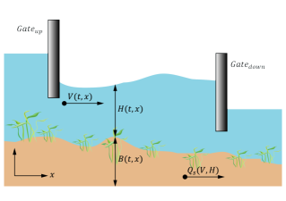
Figure 1: A sketch of the channel.

2.1 Steady-state and Linearization

A steady-state is a constant state ($H^{*}$, $V^{*}$, $B^{*})^{T}$ which satisfies the relation

$$gS_{b}H^{*}=C_{f}V^{*2}.$$

In order to linearize the model, we define the deviation of the state $\big{(}H(t,x),V(t,x)$, $B(t,x)\big{)}^{T}$ with respect to the steady-state:

$$\left(\begin{array}[]{c}h(x,t)\\ u(x,t)\\ b(x,t)\end{array}\right)=\left(\begin{array}[]{c}H(x,t)-H^{*}\\ V(x,t)-V^{*}\\ B(x,t)-B^{*}\end{array}\right).$$

Then the linearized system of the SVE model (1) around a steady-state is

$$\dfrac{\partial h}{\partial t}+V^{*}\frac{\partial h}{\partial x}+H^{*}\frac{\partial{u}}{\partial x}=0$$ (2a)

$$\dfrac{\partial{u}}{\partial t}+V^{*}\frac{\partial{u}}{\partial x}+g\frac{\partial h}{\partial x}+g\frac{\partial b}{\partial x}=C_{f}\frac{V^{*2}}{H^{*2}}h-2C_{f}\frac{V^{*}}{H^{*}}u$$ (2b)

$$\dfrac{\partial b}{\partial t}+aV^{*2}\frac{\partial{u}}{\partial x}=0.$$ (2c)

2.2 Characteristic (Riemann) coordinates

In the matrix form, the linearized model (2) can be written as

$$\displaystyle{\frac{\partial W}{\partial t}+\bm{A}(W^{*})\frac{\partial W}{\partial x}=\bm{B}(W^{*})W},$$ (3)

where

$$W=\left(\begin{array}[]{c}{h}\\ {u}\\ {b}\\ \end{array}\right),\leavevmode\nobreak\ \bm{A}(W^{*})=\left(\begin{array}[]{ccc}{V^{*}}&{H^{*}}&{0}\\ {g}&{V^{*}}&{g}\\ {0}&\displaystyle aV^{*2}&{0}\end{array}\right),$$

$$\bm{B}(W^{*})=\left(\begin{array}[]{ccc}{0}&{0}&{0}\\ \displaystyle{C_{f}\frac{V^{*2}}{H^{*2}}}&\displaystyle{-2C_{f}\frac{V^{*}}{H^{*}}}&{0}\\ {0}&{0}&{0}\end{array}\right).$$

The dimensionless Froude number is defined as

$$Fr=\frac{V^{*}}{\sqrt{gH*}}.$$

Exact, but rather complicated expressions of the eigenvalues of $\bm{A}(W^{*})$ can be obtained by using the Cardano-Vieta method, see [17]. Once the eigenvalues $\lambda_{i}$ of the matrix $\bm{A}(W^{*})$ are obtained, the corresponding left eigenvectors can be computed as

$$L_{k} ={\frac{1}{(\lambda_{k}-\lambda_{i})(\lambda_{k}-\lambda_{j})}}\left(\begin{array}[]{c}{(V^{*}-\lambda_{i})(V^{*}-\lambda_{j})+gH^{*}}\\ {H^{*}\lambda_{k}}\\ {gH^{*}}\\ \end{array}\right),$$ (7)

$${\rm{for}}\leavevmode\nobreak\ k\neq i\neq j\;\in\;\left\{1,2,3\right\}.$$ (8)

We multiply (3) by $L^{T}_{k}$ in order to rewrite the model in terms of the characteristic coordinates $\psi_{k}$ ($k=1,2,3$). Then we obtain

$$\frac{\partial\Phi_{k}}{\partial t}+\lambda_{k}\frac{\partial\Phi_{k}}{\partial x}=L^{T}_{k}\bm{B}W,{\rm{for}}\leavevmode\nobreak\ k=1,2,3,$$ (9)

where

$$\Phi_{k}= \dfrac{1}{(\lambda_{k}-\lambda_{i})(\lambda_{k}-\lambda_{j})}\left[\big{(}(V^{*}-\lambda_{i})(V^{*}-\lambda_{j})\right.$$

$$\left.+gH^{*}\big{)}h+H^{*}\lambda_{k}u+gH^{*}b\right].$$ (10)

For the sake of simplicity, we introduce the following notation $r_{k}$:

$$r_{k}=C_{f}\frac{V^{*}}{H^{*}}\frac{\lambda_{k}}{(\lambda_{k}-\lambda_{i})(\lambda_{k}-\lambda_{j})}.$$

Some computations yields the following writing for equation (9):

$$\dfrac{\partial\xi_{k}}{\partial t}+\lambda_{k}\frac{\partial\xi_{k}}{\partial x}+\sum_{s=1}^{3}(2\lambda_{s}- 3V^{*})r_{s}\xi_{s}=0,$$

$${\text{for}}\leavevmode\nobreak\ k=1,2,3,$$ (11)

where the characteristic coordinates are now defined as

$$\displaystyle{\xi_{k}=\frac{1}{r_{k}}\Phi_{k}}.$$ (12)

From (11), the linearized model (9) in characteristic form can be written as

$$\frac{\partial\bm{\xi}}{\partial t}+\bm{\Lambda}\frac{\partial\bm{\xi}}{\partial x}-\bm{M}\bm{\xi}=0,$$ (13)

where

$$\bm{\xi}=(\xi_{1},\xi_{2},\xi_{3})^{T},\quad\bm{\Lambda}=diag(\lambda_{1},\lambda_{2},\lambda_{3}),$$

$$\bm{M}=\left(\begin{array}[]{ccc}{\alpha_{1}}&{\alpha_{2}}&{\alpha_{3}}\\ {\alpha_{1}}&{\alpha_{2}}&{\alpha_{3}}\\ {\alpha_{1}}&{\alpha_{2}}&{\alpha_{3}}\end{array}\right),$$

with

$$\alpha_{k}=\Big{(}3V^{*}-2\lambda_{k}\Big{)}r_{k}.$$

From [17], the three eigenvalues of the matrix $\bm{A}$ are such that for a subcritical flow regime $(Fr<1)$,

$$\lambda_{1}<0<\lambda_{2}\ll\lambda_{3}$$ (14)

and for a supercritical one $(Fr>1)$,

$$\lambda_{2}<0<\lambda_{1}<\lambda_{3}$$ (15)

with $\lambda_{1}$ and $\lambda_{3}$ being the characteristic velocities of the water flow and $\lambda_{2}$ being the characteristic velocity of the sediment motion. Obviously, the sediment motion is much slower than the water flow.

2.3 Change of notations

Hereafter, we consider the case where the flow regime is subcritical and adopt the following notations: $v(t,x)=\xi_{1}(t,x)$, $u_{1}(t,x)=\xi_{2}(t,x)$, $u_{2}(t,x)=\xi_{3}(t,x)$ and coefficients (characteristic velocities) $\lambda_{1}=-\mu$, $\gamma_{1}=\lambda_{2}$ and $\gamma_{2}=\lambda_{3}$. We introduce also the vector $\bm{u}=(u_{1},u_{2})^{tr}$, the coefficients $\eta_{\rm{j}}=\alpha_{\rm{j+1}}$ for $j=1,\,2$ and the matrix

$$\bm{\sigma}=\left(\begin{array}[]{cc}{\alpha_{2}}&{\alpha_{3}}\\ {\alpha_{2}}&{\alpha_{3}}\end{array}\right).$$ (18)

With the new variables, the set of equation (13) writes as:

$$\partial_{t}u_{1}+\gamma_{1}\partial_{x}u_{1}=\sigma_{{11}}u_{1}+\sigma_{{12}}u_{\rm{2}}+\alpha_{1}v$$ (19a)

$$\partial_{t}u_{2}+\gamma_{2}\partial_{x}u_{2}=\sigma_{{21}}u_{1}+\sigma_{{22}}u_{\rm{2}}+\alpha_{1}v$$ (19b)

$$\partial_{t}v-\mu\partial_{x}v=\eta_{1}u_{1}+\eta_{2}u_{2}+\alpha_{1}v.$$ (19c)

Introduce the variable

$$w(t,x)=v(t,x)\exp\left(-\frac{\alpha_{1}}{\mu}x\right),$$

then the system (19) is transformed into

$$\partial_{t}u_{1}+\gamma_{1}\partial_{x}u_{1}= \sigma_{\rm{11}}u_{1}+\sigma_{\rm{12}}u_{2}$$

$$+\alpha_{1}\exp\left(\frac{\alpha_{1}}{\mu}x\right)w$$ (20a)

$$\partial_{t}u_{2}+\gamma_{2}\partial_{x}u_{2}= \sigma_{\rm{21}}u_{1}+\sigma_{\rm{22}}u_{2}$$

$$+\alpha_{1}\exp\left(\frac{\alpha_{1}}{\mu}x\right)w$$ (20b)

$$\partial_{t}w-\mu\partial_{x}w= \eta_{1}\exp\left(\frac{\alpha_{1}}{\mu}x\right)u_{1}$$

$$+\eta_{2}\exp\left(\frac{\alpha_{1}}{\mu}x\right)u_{2}.$$ (20c)

We rewrite this system as:

$$\partial_{t}u_{1}+\gamma_{1}\partial_{x}u_{1}=\sigma_{11}u_{1}+\sigma_{12}u_{2}+\alpha(x)w$$ (21a)

$$\partial_{t}u_{2}+\gamma_{2}\partial_{x}u_{2}=\sigma_{21}u_{1}+\sigma_{22}u_{2}+\alpha(x)w$$ (21b)

$$\partial_{t}w-\mu\partial_{x}w=\theta_{1}(x)u_{1}+\theta_{2}(x)u_{2}$$ (21c)

with $\alpha(x)=\alpha_{1}\exp\left(\frac{\alpha_{1}}{\mu}x\right)$ and $\theta_{\rm{j}}(x)=\alpha_{\rm{j+1}}\exp\left(\frac{\alpha_{1}}{\mu}x\right)$ for $j=1,\,2$.

To close the writing of the system (21), we enclose to it the following boundary and initial conditions

$$u_{\rm{i}}(t,0)=q_{\rm{i}}w(t,0)\quad\text{for }{\rm{i}}=1,2,$$ (22a)

$$w(t,1)=\rho_{1}u_{1}(t,1)+\rho_{2}u_{2}(t,1)+U(t),$$ (22b)

$$w(0,x)=w^{0}(x),\;u_{\rm{i}}(0,x)=u_{i}^{0}(x)\quad\text{for }{\rm{i}}=1,2.$$ (22c)

Remark 1.

Let us mention that in the case where the flow regime is supercritical, the following changes of variable will be considered (instead of the previous one) $v(t,x)=\xi_{2}(t,x)$, $u_{1}(t,x)=\xi_{1}(t,x)$, $u_{2}(t,x)=\xi_{3}(t,x)$ and coefficients $\lambda_{2}=-\mu$, $\gamma_{1}=\lambda_{1}$ and $\gamma_{2}=\lambda_{3}$.

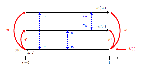
Figure 2: Schematic steep of the hyperbolic system. The internal coupling between the states in the system and boundary conditions are depicted.

As in [9], $u_{1}$, $u_{2}$ and $w$ are the distributed states and $U(t)$ is the control input as shown in Figure 2. The measured output is given by: $w(t,0)=y(t)$.

3 Full State Controller Design

3.1 Backstepping transformation and target system

Consider the following backstepping transformation

$$\psi_{i}(t,x)=u_{\rm{i}}(t,x)\text{ for }i=1,\,2$$ (23)

$$\chi(t,x)=w(t,x)-\int_{0}^{x}k_{1}(x,\xi)u_{1}(t,\xi)\,d\xi$$

$$-\int_{0}^{x}k_{2}(x,\xi)u_{2}(t,\xi)\,d\xi-\int_{0}^{x}k_{3}(x,\xi)w(t,\xi)\,d\xi.$$ (24)

We now seek a sufficient condition on the functions $k_{\rm{i}}$ such that the transformation (23)-(24) maps the system (21)-(22) to the target system

$$\partial_{t}\psi_{1}+\gamma_{1}\partial_{x}\psi_{1}= \sigma_{11}\psi_{1}+\sigma_{12}\psi_{2}+\alpha(x)\chi$$

$$+\int_{0}^{x}c_{11}(x,\xi)\psi_{1}(t,\xi)\,d\xi$$

$$+\int_{0}^{x}c_{12}(x,\xi)\psi_{2}(t,\xi)\,d\xi$$

$$+\int_{0}^{x}\kappa_{1}(x,\xi)\chi(t,\xi)\,d\xi$$ (25a)

$$\partial_{t}\psi_{2}+\gamma_{2}\partial_{x}\psi_{2}= \sigma_{21}\psi_{1}+\sigma_{22}\psi_{2}+\alpha(x)\chi$$

$$+\int_{0}^{x}c_{21}(x,\xi)\psi_{1}(t,\xi)\,d\xi$$

$$+\int_{0}^{x}c_{22}(x,\xi)\psi_{2}(t,\xi)\,d\xi$$

$$+\int_{0}^{x}\kappa_{2}(x,\xi)\chi(t,\xi)\,d\xi$$ (25b)

$$\partial_{t}\chi-\mu\partial_{x}\chi= 0$$ (25c)

with the following boundary conditions:

$$\psi_{\rm{i}}(t,0)=q_{\rm{i}}\chi(t,0)\text{ for }i=1,\,2\text{ and }\chi(t,1)=0.$$ (26)

This dynamic is schematically represented on Figure . In the system (25), $c_{\rm{ij}}(\cdot)$ and $\kappa_{\rm{i}}(\cdot)$ are functions to be determined on the triangular domain

$$\mathbb{T}=\Big{\{}(x,\xi)\in\mathbb{R}^{2}|\;0\leq\xi\leq x\leq 1\Big{\}}.$$

The system (25)-(26) is designed as a copy of the original dynamics with the coupling term in (21c) removed. As will be shown later, the new terms in (25a) and (25b) are necessary for the design but they will not affect the stability.

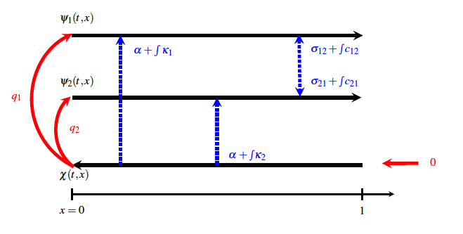
Figure 3: Representation of the target system.

A sufficient condition for the transformation (23)-(24) to map the original system (21) into the target system (25) is that the kernels $k_{\rm{i}}$ satisfy the following system of first order hyperbolic PDEs:

$$\mu\partial_{x}k_{1}(x,\xi)-\gamma_{1}\partial_{\xi}k_{1}(x,\xi)$$

$$\quad=\sigma_{11}k_{1}(x,\xi)+\sigma_{21}k_{2}(x,\xi)+\theta_{1}(\xi)k_{3}(x,\xi)$$ (27a)

$$\mu\partial_{x}k_{2}(x,\xi)-\gamma_{2}\partial_{\xi}k_{2}(x,\xi)$$

$$\quad=\sigma_{12}k_{1}(x,\xi)+\sigma_{22}k_{2}(x,\xi)+\theta_{2}(\xi)k_{3}(x,\xi)$$ (27b)

$$\mu\partial_{x}k_{3}(x,\xi)+\mu\partial_{\xi}k_{3}(x,\xi)$$

$$\quad=\alpha(\xi)k_{1}(x,\xi)+\alpha(\xi)k_{2}(x,\xi)$$ (27c)

with the following boundary conditions:

$$k_{1}(x,x)=-\frac{\theta_{1}(x)}{\gamma_{1}+\mu},\leavevmode\nobreak\ k_{2}(x,x)=-\frac{\theta_{2}(x)}{\gamma_{2}+\mu},$$ (28a)

$$\mu k_{3}(x,0)=q_{1}\gamma_{1}k_{1}(x,0)+q_{2}\gamma_{2}k_{2}(x,0).$$ (28b)

The existence, uniqueness and continuity of the solutions to the system (27) with boundary conditions (28) are assessed by Theorem 5.3 in [9].

Besides, plugging (23)-(24) into (25) and using (21)-(22) yields for $i=1,\,2$,

$$0= \int_{0}^{x}\Big{[}\alpha(\xi)k_{1}(x,\xi)-c_{i1}(x,\xi)$$

$$\qquad+\int_{\xi}^{x}\kappa_{1}(x,s)k_{1}(s,\xi)\,ds\Big{]}u_{1}(\xi)\,d\xi$$

$$+\int_{0}^{x}\Big{[}\alpha(\xi)k_{2}(x,\xi)-c_{i2}(x,\xi)$$

$$\qquad+\int_{\xi}^{x}\kappa_{2}(x,s)k_{2}(s,\xi)\,ds\Big{]}u_{2}(\xi)\,d\xi$$ (29)

$$+\int_{0}^{x}\Big{[}\alpha(\xi)k_{3}(x,\xi)-\kappa_{\rm i}(x,\xi)$$

$$\qquad+\int_{\xi}^{x}\kappa_{\rm i}(x,s)k_{3}(s,\xi)\,ds\Big{]}w(\xi)\,d\xi.$$ (30)

The coefficients $\kappa_{\rm{i}}$ can be chosen to satisfy the following integral equation for $i=1,\,2$

$$\kappa_{\rm{i}}(x,\xi)=\alpha(x)k_{3}(x,\xi)+\int_{\xi}^{x}\kappa_{\rm i}(x,s)k_{3}(s,\xi)\,ds,$$ (31)

and the coefficients $c_{\rm{ij}}$ can be chosen such that

$$c_{\rm{ij}}(x,\xi)=\alpha(x)k_{\rm{j}}(x,\xi) +\int_{\xi}^{x}\kappa_{i}(x,s)k_{\rm{j}}(s,\xi)\,ds$$

$$\text{for}\;i,\,j=1,\,2$$ (32)

under the fact that the $k_{\rm i}$ exist and are sufficiently smooth.

3.2 Inverse transformation and control law

To ensure that the target system and the closed-loop system have equivalent stability properties, the transformation (23)-(24) has to be invertible. Since $\psi_{\rm i}=u_{\rm i}$, for $i=1,\,2$, the transformation (24) can be rewritten as

$$\chi(t,x)+\int_{0}^{x}k_{1}(x,\xi)\psi_{1}(t,\xi)\,d\xi$$

$$+\int_{0}^{x}k_{2}(x,\xi)\psi_{2}(t,\xi)\,d\xi$$

$$\leavevmode\nobreak\ \leavevmode\nobreak\ \leavevmode\nobreak\ \leavevmode\nobreak\ =w(t,x)-\int_{0}^{x}k_{3}(x,\xi)w(t,\xi)\,d\xi.$$ (33)

Let us define

$$\Gamma(t,x)= \chi(t,x)+\int_{0}^{x}k_{1}(x,\xi)\psi_{1}(t,\xi)\,d\xi$$

$$+\int_{0}^{x}k_{2}(x,\xi)\psi_{2}(t,\xi)\,d\xi$$ (34)

Since $k_{3}$ is continuous by Theorem $5.3$ in [9], there exists a unique continuous inverse kernel $l_{3}$ defined on $\mathbb{T}$, such that

$$w(t,x)=\Gamma(t,x)+\int_{0}^{x}l_{3}(x,\xi)\Gamma(t,\xi)\,d\xi,$$ (35)

which yields the following inverse transformation Since $\psi_{\rm i}=u_{\rm i}$, for $i=1,\,2$, we could get the following relation from the first two equalities of $(\ref{newvar3})$ and $(\ref{targetsys})$:

$$\alpha(x)w=\alpha(x)\chi+\int_{0}^{x}c_{11}(x,\xi)\psi_{1}(t,\xi)\,d\xi$$

$$+\int_{0}^{x}c_{12}(x,\xi)\psi_{2}(t,\xi)\,d\xi+\int_{0}^{x}\kappa_{1}(x,\xi)\chi(t,\xi)\,d\xi.$$ (36)

Thus, we could write the following

$$w(t,x)=\chi(t,x)+\int_{0}^{x}l_{1}(x,\xi)\psi_{1}(t,\xi)\,d\xi$$

$$+\int_{0}^{x}l_{2}(x,\xi)\psi_{2}(t,\xi)\,d\xi+\int_{0}^{x}l_{3}(x,\xi)\chi(t,\xi)\,d\xi,$$ (37)

where for $i=1,\,2$,

$$l_{\rm i}(x,\xi)=k_{\rm i}(t,\xi)+\int_{\xi}^{x}k_{\rm i}(x,\xi)l_{3}(\xi,s)\,ds.$$ (38)

Thus, the control law $U(t)$ can be obtained by plugging the transformation (24) into (21). Readily, $\chi(t,1)=0$ implies that

$$U(t)= -\rho_{1}u_{1}(t,1)-\rho_{2}u_{2}(t,1)$$

$$+\int_{0}^{1}\Big{[}k_{1}(1,\xi)u_{1}(x,\xi)$$

$$+k_{2}(1,\xi)u_{2}(x,\xi)+k_{3}(1,\xi)w(1,\xi)\Big{]}\,d\xi.$$ (39)

The $k_{i}$ in the integral term designate the kernel functions and satisfy the system (27)-(28).

3.3 Stability of the target system and the closed-loop control system

We first prove exponential stability of the target system (25)-(26).

Lemma 1.

For any given initial condition $(\psi^{0}_{1},\ \psi^{0}_{2},\ \chi^{0})^{T}\,\in\,\left(\mathcal{L}^{2}([0,1])\right)^{3}$ and under the assumption that $c_{\rm{ij}},\leavevmode\nobreak\ \kappa_{\rm{i}}\,\in\mathcal{C}(\mathbb{T})$, the equilibrium $(\psi_{1},\ \psi_{2},\ \chi)^{T}=(0,\ 0,\ 0)^{T}$ of the target system (25)-(26) is $\mathcal{L}^{2}$-exponentially stable.

The stability proof is based on the time differentiation of the following Lyapunov function:

$$V_{1}(t)= \int_{0}^{1}a_{1}e^{-\delta_{1}x}\left(\frac{\psi^{2}_{1}(t,x)}{\gamma_{1}}+\frac{\psi^{2}_{2}(t,x)}{\gamma_{2}}\right)dx$$

$$+\int_{0}^{1}\frac{1+x}{\mu}\chi^{2}(t,x)dx,$$ (40)

where $a_{1}$ and $\delta_{1}$ are strictly positive parameters to be determined.

Differentiating this function with respect to time, we get:

$$\dot{V}_{1}(t)= 2\int_{0}^{1}a_{1}e^{-\delta_{1}x}\left(\frac{\psi_{1}\partial_{t}\psi_{1}}{\gamma_{1}}+\frac{\psi_{2}\partial_{t}\psi_{2}}{\gamma_{2}}\right)dx$$

$$+2\int_{0}^{1}\frac{1+x}{\mu}\chi\partial_{t}\chi dx.$$ (41)

By taking into account the target system (25)-(26) and integrating by parts, we have

$$\dot{V}_{1}(t)= \Big{[}-a_{1}e^{-\delta_{1}x}(\psi^{2}_{1}(t,x)+\psi^{2}_{2}(t,x))$$

$$\leavevmode\nobreak\ \leavevmode\nobreak\ \leavevmode\nobreak\ \leavevmode\nobreak\ \leavevmode\nobreak\ \leavevmode\nobreak\ +(1+x)\chi^{2}(t,x)\Big{]}_{0}^{1}$$

$$-\int_{0}^{1}\chi^{2}(t,x)\ dx+\int_{0}^{1}a_{1}e^{-\delta_{1}x}$$

$$\times\Psi^{T}(t,x)\left(-\delta_{1}I_{2}+2\bm{\Gamma}_{inv}\bm{\sigma}\right)\Psi(t,x)\ dx$$

$$+2\int_{0}^{1}a_{1}e^{-\delta_{1}x}\Psi^{T}(t,x)\bm{\Gamma}_{inv}\bm{\alpha}(x)\chi(t,x)\ dx$$

$$+2\int_{0}^{1}a_{1}e^{-\delta_{1}x}\int_{0}^{x}\Psi^{T}(t,x)\bm{\Gamma}_{inv}$$

$$\times\left(\bm{C}(x,\xi)\Psi(t,\xi)\right.\left.+K(x,\xi)\chi(t,\xi)\right)\ d\xi\ dx,$$

where the matrix $\bm{\sigma}$ is defined in $(\ref{sigma})$, the vectors $\Psi(t,x)$, $\bm{\alpha}(x)$, $K(x,\xi)$ and the matrices $\bm{\Gamma}_{inv}$, $\bm{C}(x,\xi)$ are given by

$${\Psi}(t,x)=\left(\begin{matrix}{\psi_{1}(t,x)}\\ {\psi_{2}(t,x)}\end{matrix}\right),\leavevmode\nobreak\ \bm{\alpha}(x)=\left(\begin{matrix}\alpha(x)\\ \alpha(x)\end{matrix}\right)$$ (42)

$$K(x,\xi)=\left(\begin{matrix}{\kappa_{1}(x,\xi)}\\ {\kappa_{2}(x,\xi)}\end{matrix}\right),\bm{\Gamma}_{inv}=\left(\begin{matrix}\frac{1}{\gamma_{1}}&0\\ 0&\frac{1}{\gamma_{2}}\end{matrix}\right)$$ (43)

$$\bm{C}(x,\xi)=\left(\begin{matrix}{c_{11}}(x,\xi)&{c_{12}}(x,\xi)\\ {c_{21}}(x,\xi)&{c_{22}}(x,\xi)\end{matrix}\right).$$ (44)

Assume that for $M>0$ and $\epsilon>0$, we have

$$\|\bm{\sigma}\|,\ \|\bm{\alpha}(x)\|,\|\bm{C}(x,\xi)\|,\ \|K(x,\xi)\|\leq M,$$

$$\leavevmode\nobreak\ \leavevmode\nobreak\ \leavevmode\nobreak\ \leavevmode\nobreak\ \leavevmode\nobreak\ \leavevmode\nobreak\ \leavevmode\nobreak\ \leavevmode\nobreak\ \leavevmode\nobreak\ \leavevmode\nobreak\ \leavevmode\nobreak\ \leavevmode\nobreak\ \leavevmode\nobreak\ \leavevmode\nobreak\ \leavevmode\nobreak\ \leavevmode\nobreak\ \leavevmode\nobreak\ \leavevmode\nobreak\ \leavevmode\nobreak\ \leavevmode\nobreak\ \forall x\in[0,1],\xi\in[0,x],$$ (45)

$$\gamma_{i}(x)>\epsilon,\forall i=1,2,\forall x\in[0,1],$$ (46)

where the matrix/vector norms $\|\cdot\|$ are compatible with the other corresponding matrix/vector norms. Hence, using Young’s inequalities the following relations are derived

$$2\int_{0}^{1}a_{1}e^{-\delta_{1}x}\Psi^{T}(t,x)\bm{\Gamma}_{inv}\bm{\sigma}\Psi(t,x)\ dx$$

$$\leavevmode\nobreak\ \leavevmode\nobreak\ \leavevmode\nobreak\ \leavevmode\nobreak\ \leq 2\frac{M}{\epsilon}\int_{0}^{1}a_{1}e^{-\delta_{1}x}\Psi^{T}(t,x)\Psi(t,x)\ dx$$ (47)

$$2\int_{0}^{1}a_{1}e^{-\delta_{1}x}\Psi^{T}(t,x)\bm{\Gamma}_{inv}\bm{\alpha}(x)\chi(t,x)\ dx$$

$$\leavevmode\nobreak\ \leavevmode\nobreak\ \leavevmode\nobreak\ \leavevmode\nobreak\ \leq\int_{0}^{1}a_{1}e^{-\delta_{1}x}\left(\Psi^{T}(t,x)\bm{\Gamma}_{inv}\bm{\alpha}(x)\right.$$

$$\left.\leavevmode\nobreak\ \leavevmode\nobreak\ \leavevmode\nobreak\ \leavevmode\nobreak\ \leavevmode\nobreak\ \leavevmode\nobreak\ \leavevmode\nobreak\ \leavevmode\nobreak\ \leavevmode\nobreak\ \leavevmode\nobreak\ \leavevmode\nobreak\ \leavevmode\nobreak\ \leavevmode\nobreak\ \leavevmode\nobreak\ \times\bm{\alpha}^{T}(x)\bm{\Gamma}_{inv}\Psi(t,x)+\chi^{2}(t,x)\right)dx$$

$$\leavevmode\nobreak\ \leavevmode\nobreak\ \leavevmode\nobreak\ \leavevmode\nobreak\ \leq a_{1}\left(\frac{M}{\epsilon}\right)^{2}\int_{0}^{1}e^{-\delta_{1}x}\Psi^{T}(t,x)\Psi(t,x)dx$$

$$\leavevmode\nobreak\ \leavevmode\nobreak\ \leavevmode\nobreak\ \leavevmode\nobreak\ \leavevmode\nobreak\ \leavevmode\nobreak\ \leavevmode\nobreak\ \leavevmode\nobreak\ +a_{1}\int_{0}^{1}e^{-\delta_{1}x}\chi^{2}(t,x)dx$$ (48)

and

$$2\int_{0}^{1}a_{1}e^{-\delta_{1}x}\int_{0}^{x}\Psi^{T}(t,x)\bm{\Gamma}_{inv}\bm{C}(x,\xi)\Psi(t,\xi)\ d\xi\ dx$$

$$\leq\frac{M}{\epsilon}\int_{0}^{1}a_{1}e^{-\delta_{1}x}\int_{0}^{x}\left(\Psi^{T}(t,x)\Psi(t,x)\right.$$

$$\leavevmode\nobreak\ \leavevmode\nobreak\ \leavevmode\nobreak\ \leavevmode\nobreak\ \left.+\Psi^{T}(t,\xi)\Psi(t,\xi)\right)d\xi dx$$

$$=\frac{M}{\epsilon}\int_{0}^{1}a_{1}e^{-\delta_{1}x}x\Psi^{T}(t,x)\Psi(t,x)dx$$

$$\leavevmode\nobreak\ \leavevmode\nobreak\ \leavevmode\nobreak\ \leavevmode\nobreak\ +\frac{M}{\delta_{1}\epsilon}\int_{0}^{1}a_{1}\left(e^{-\delta_{1}x}-e^{-\delta_{1}}\right)\Psi^{T}(t,x)\Psi(t,x)dx$$

$$\leq a_{1}\int_{0}^{1}e^{-\delta_{1}x}\left(\frac{M}{\epsilon}x+\frac{M}{\delta_{1}\epsilon}\right)\Psi^{T}(t,x)\Psi(t,x)dx$$ (49)

$$2\int_{0}^{1}a_{1}e^{-\delta_{1}x}\int_{0}^{x}\Psi^{T}(t,x)\bm{\Gamma}_{inv}K(x,\xi)\chi(t,\xi)\ d\xi\ dx$$

$$\leq a_{1}\int_{0}^{1}e^{-\delta_{1}x}\int_{0}^{x}\left(\Psi^{T}(t,x)\bm{\Gamma}_{inv}K(x,\xi)\right.$$

$$\leavevmode\nobreak\ \leavevmode\nobreak\ \leavevmode\nobreak\ \leavevmode\nobreak\ \left.\times K^{T}(x,\xi)\bm{\Gamma}_{inv}\Psi(t,x)+\chi^{2}(t,\xi)\right)d\xi dx$$

$$\leq a_{1}\left(\frac{M}{\epsilon}\right)^{2}\int_{0}^{1}e^{-\delta_{1}x}x\Psi^{T}(t,x)\Psi(t,x)dx$$

$$\leavevmode\nobreak\ \leavevmode\nobreak\ \leavevmode\nobreak\ \leavevmode\nobreak\ +a_{1}\frac{1}{\delta_{1}}\int_{0}^{1}e^{-\delta_{1}x}\chi^{2}(t,x)dx.$$ (50)

Thus, using the boundary conditions (26), we obtain the following inequality

$$\dot{V}_{1}(t)\leq \left(a_{1}\sum_{i=1}^{2}q_{i}^{2}-1\right)\chi^{2}(t,0)$$

$$-\int_{0}^{1}\left(1-a_{1}(1+\frac{1}{\delta_{1}})e^{-\delta_{1}x}\right)\chi^{2}(t,x)\ dx$$

$$-a_{1}\int_{0}^{1}e^{-\delta_{1}x}\Psi^{T}(t,x)P_{1}(x)\Psi(t,x)\ dx,$$ (51)

where

$$P(x)= \left(\delta_{1}-2\frac{M}{\epsilon}-\frac{M}{\epsilon}x-2\left(\frac{M}{\epsilon}\right)^{2}-\frac{M}{\delta_{1}\epsilon}\right)I_{2}$$

$$-2\bm{\Gamma}_{inv}\bm{\sigma}.$$ (52)

First, we choose the tuning parameter $\delta_{1}>0$ sufficiently large so that the matrix $P(x),x\in[0,1]$ is positive definite. Then, by choosing

$$0<a_{1}<\min\left\{\frac{1}{\sum\limits_{i=1}^{2}q_{i}^{2}},\frac{\delta_{1}}{\delta_{1}+1}\right\},$$ (53)

we could derive exponential stability of the target system.

Then, from the continuity and invertibility of the backstepping transformation (23)-(24), we could derive equivalence between the original system (21) (with the boundary and initial conditions (22) and the control law (39)) and the target system (25)-(26). Thus, the following theorem is proved.

Theorem 1.

Consider the system (21) with the boundary and initial conditions (22) and the control law (39). Then under the assumptions that the initial data are in $\left(\mathcal{L}^{2}([0,1])\right)^{3}$, the origin is exponentially stable in the $\mathcal{L}^{2}$ sense.

4 Backstepping Observer Design

The feedback controller (39) requires a full state measurement across the spatial domain. In this section we are interested in the design of a boundary state observer for estimation of the distributed states of the system (21)-(22) over the whole spatial domain using the measured output $w(t,0)=y(t)$. The observer

$$\partial_{t}\hat{u}_{1}+\gamma_{1}\partial_{x}\hat{u}_{1}=\sigma_{11}\hat{u}_{1}+\sigma_{12}\hat{u}_{2}+\alpha(x)\hat{w}$$

$$\leavevmode\nobreak\ \leavevmode\nobreak\ \leavevmode\nobreak\ \leavevmode\nobreak\ \leavevmode\nobreak\ \leavevmode\nobreak\ \leavevmode\nobreak\ \leavevmode\nobreak\ \leavevmode\nobreak\ \leavevmode\nobreak\ \leavevmode\nobreak\ \leavevmode\nobreak\ \leavevmode\nobreak\ \leavevmode\nobreak\ \leavevmode\nobreak\ \leavevmode\nobreak\ \leavevmode\nobreak\ \leavevmode\nobreak\ \leavevmode\nobreak\ -p_{1}(x)[y(t)-\hat{w}(t,0)]$$ (54a)

$$\partial_{t}\hat{u}_{2}+\gamma_{2}\partial_{x}\hat{u}_{2}=\sigma_{21}\hat{u}_{1}+\sigma_{22}\hat{u}_{2}+\alpha(x)\hat{w}$$

$$\leavevmode\nobreak\ \leavevmode\nobreak\ \leavevmode\nobreak\ \leavevmode\nobreak\ \leavevmode\nobreak\ \leavevmode\nobreak\ \leavevmode\nobreak\ \leavevmode\nobreak\ \leavevmode\nobreak\ \leavevmode\nobreak\ \leavevmode\nobreak\ \leavevmode\nobreak\ \leavevmode\nobreak\ \leavevmode\nobreak\ \leavevmode\nobreak\ \leavevmode\nobreak\ \leavevmode\nobreak\ \leavevmode\nobreak\ \leavevmode\nobreak\ -p_{2}(x)[y(t)-\hat{w}(t,0)]$$ (54b)

$$\partial_{t}\hat{w}-\mu\partial_{x}\hat{w}=\theta_{1}(x)\hat{u}_{1}+\theta_{2}(x)\hat{u}_{2}$$

$$\leavevmode\nobreak\ \leavevmode\nobreak\ \leavevmode\nobreak\ \leavevmode\nobreak\ \leavevmode\nobreak\ \leavevmode\nobreak\ \leavevmode\nobreak\ \leavevmode\nobreak\ \leavevmode\nobreak\ \leavevmode\nobreak\ \leavevmode\nobreak\ \leavevmode\nobreak\ \leavevmode\nobreak\ \leavevmode\nobreak\ \leavevmode\nobreak\ \leavevmode\nobreak\ \leavevmode\nobreak\ \leavevmode\nobreak\ \leavevmode\nobreak\ -p_{3}(x)[y(t)-\hat{w}(t,0)],$$ (54c)

where $(\hat{u}_{1},\ \hat{u}_{2},\ \hat{w})^{T}$ is the estimated state vector, consists of a copy of the plant plus an output injection and mimics the well-known finite dimensional observer format. The functions $\theta_{\rm{j}}(x)=\alpha_{\rm{j+1}}$ for $j=1,\,2$ and $\alpha(x)$ are the ones defined for the transformed system (21). The following boundary conditions have to be considered:

$$\hat{u}_{\rm{i}}(t,0)=q_{\rm{i}}y(t)\quad\text{for }{\rm{i}}=1,2$$ (55a)

$$\hat{w}(t,1)=\rho_{1}\hat{u}_{1}(t,1)+\rho_{2}\hat{u}_{2}(t,1)+U(t).$$ (55b)

Our objective is to find $p_{1}(x)$, $p_{2}(x)$ and $p_{3}(x)$ such that the estimated state vector $(\hat{w},\ \hat{u}_{1},\ \hat{u}_{2})$ converges to the real state vector $(w,\ u_{1},\ u_{2})$ in finite time. Defining

$$\left(\begin{array}[]{ccc}\tilde{w}&\tilde{u}_{1}&\tilde{u}_{2}\\ \end{array}\right)^{T}=\left(\begin{array}[]{ccc}w-\hat{w}&u_{1}-\hat{u}_{1}&u_{2}-\hat{u}_{2}\\ \end{array}\right)^{T}$$ (58)

as the error variable vector, we obtain the following error system

$$\partial_{t}\tilde{w}-\mu\partial_{x}\tilde{w}= \theta_{1}(x)\tilde{u}_{1}+\theta_{2}(x)\tilde{u}_{2}+p_{3}(x)\tilde{w}(t,0)$$ (59a)

$$\partial_{t}\tilde{u}_{1}+\gamma_{1}\partial_{x}\tilde{u}_{1}= \sigma_{11}\tilde{u}_{1}+\sigma_{12}\tilde{u}_{2}+\alpha(x)\tilde{w}$$

$$+p_{1}(x)\tilde{w}(t,0)$$ (59b)

$$\partial_{t}\tilde{u}_{2}+\gamma_{2}\partial_{x}\tilde{u}_{2}= \sigma_{21}\tilde{u}_{1}+\sigma_{22}\tilde{u}_{2}+\alpha(x)\tilde{w}$$

$$+p_{2}(x)\tilde{w}(t,0)$$ (59c)

with the boundary conditions

$$\tilde{w}(t,1)=\rho_{1}\tilde{u}_{1}(t,1)+\rho_{2}\tilde{u}_{2}(t,1),$$ (60a)

$$\tilde{u}_{\rm{i}}(t,0)=0\quad\text{for }{\rm{i}}=1,2.$$ (60b)

4.1 Backstepping transformation and the target error system

Similarly to the controller design, we use the following invertible backstepping transformation

$$\tilde{u}_{\rm i}(t,x)=\tilde{\pi}_{\rm i}(t,x)+\int_{0}^{x}m_{\rm i}(x,\xi)\tilde{\phi}(t,\xi)\,d\xi$$ (61a)

$$\leavevmode\nobreak\ \leavevmode\nobreak\ \leavevmode\nobreak\ \leavevmode\nobreak\ \leavevmode\nobreak\ \leavevmode\nobreak\ \leavevmode\nobreak\ \leavevmode\nobreak\ \leavevmode\nobreak\ \leavevmode\nobreak\ \leavevmode\nobreak\ \leavevmode\nobreak\ \leavevmode\nobreak\ \leavevmode\nobreak\ \leavevmode\nobreak\ \leavevmode\nobreak\ \leavevmode\nobreak\ \leavevmode\nobreak\ \leavevmode\nobreak\ \leavevmode\nobreak\ \leavevmode\nobreak\ \leavevmode\nobreak\ \leavevmode\nobreak\ \leavevmode\nobreak\ \leavevmode\nobreak\ \leavevmode\nobreak\ \leavevmode\nobreak\ \leavevmode\nobreak\ \leavevmode\nobreak\ \quad\rm{for}\leavevmode\nobreak\ {\rm{i}}=1,2$$

$$\tilde{w}(t,x)=\tilde{\phi}(t,x)+\int_{0}^{x}m_{\rm 3}(x,\xi)\tilde{\phi}(t,\xi)\,d\xi,$$ (61b)

where the kernels $m_{\rm{i}}(\cdot)\ \text{ for }i=1,\,2,\,3$ are defined in the triangular domain $\mathbb{T}$ to map the error system (59)-(60) into the following exponentially stable target system

$$\partial_{t}\tilde{\pi}_{1}+\gamma_{1}\partial_{x}\tilde{\pi}_{1}=\sigma_{11}\tilde{\pi}_{1}+\sigma_{12}\tilde{\pi}_{2}$$

$$+\int_{0}^{x}g_{11}(x,\xi)\tilde{\pi}_{1}(t,\xi)\,d\xi+\int_{0}^{x}g_{12}(x,\xi)\tilde{\pi}_{2}(t,\xi)\,d\xi$$ (62a)

$$\partial_{t}\tilde{\pi}_{2}+\gamma_{2}\partial_{x}\tilde{\pi}_{2}=\sigma_{21}\tilde{\pi}_{1}+\sigma_{22}\tilde{\pi}_{2}$$

$$+\int_{0}^{x}g_{21}(x,\xi)\tilde{\pi}_{1}(t,\xi)\,d\xi+\int_{0}^{x}g_{22}(x,\xi)\tilde{\pi}_{2}(t,\xi)\,d\xi$$ (62b)

$$\partial_{t}\tilde{\phi}-\mu\partial_{x}\tilde{\phi}=\theta_{1}(x)\tilde{\pi}_{1}+\theta_{2}(x)\tilde{\pi}_{2}$$

$$+\int_{0}^{x}h_{1}(x,\xi)\tilde{\pi}_{1}(t,\xi)\,d\xi+\int_{0}^{x}h_{2}(x,\xi)\tilde{\pi}_{2}(t,\xi)\,d\xi$$ (62c)

with the boundary conditions

$$\tilde{\pi}_{\rm{i}}(t,0)=0\text{ for }i=1,\,2$$ (63a)

$$\tilde{\phi}(t,1)=\rho_{1}\tilde{\pi}_{1}(t,1)+\rho_{2}\tilde{\pi}_{2}(t,1).$$ (63b)

Here the functions $g_{ij}$ and $h_{i}$ have to be determined on the triangular domain $\mathcal{T}$. As previously, we are attempting to find some sufficient condition for the kernels to match the target system. Differentiating the transformations (61) in time and space and substituting the results into (59) with the help of (62), the following PDEs are derived for the kernels

$$\gamma_{1}\partial_{x}m_{1}-\mu\partial_{\xi}m_{1} =\sigma_{11}m_{1}+\sigma_{12}m_{2}+\alpha(x)m_{3},$$ (64a)

$$\gamma_{2}\partial_{x}m_{2}-\mu\partial_{\xi}m_{2} =\sigma_{21}m_{1}+\sigma_{22}m_{2}+\alpha(x)m_{3},$$ (64b)

$$\mu\partial_{x}m_{3}+\mu\partial_{\xi}m_{3} =-\theta_{1}(x)m_{1}-\theta_{2}(x)m_{2}.$$ (64c)

To close the writing of the above system, the following boundary conditions are imposed:

$$m_{1}(x,x)=\frac{1}{\gamma_{1}+\mu}\alpha(x)$$ (65a)

$$m_{2}(x,x)=\frac{1}{\gamma_{2}+\mu}\alpha(x)$$ (65b)

$$m_{3}(1,\xi)=\rho_{1}m_{1}(1,\xi)+\rho_{2}m_{2}(1,\xi).$$ (65c)

The observer gains are defined by

$$p_{i}(x)=\mu m_{i}(x,0)\text{ for }i=1,\,2,\ 3,$$ (66)

and the integral coupling coefficients are defined by the following equations:

$$h_{i}(x,\xi)=-\theta(\xi)m_{3}(x,\xi)$$

$$-\int_{\xi}^{x}m_{3}(x,s)h_{i}(s,\xi)\,ds,\leavevmode\nobreak\ \rm{for}\leavevmode\nobreak\ i=1,\,2,$$ (67a)

$$g_{i,j}(x,\xi)=-\theta_{j}(\xi)m_{i}(x,\xi)$$

$$-\int_{\xi}^{x}m_{i}(x,s)h_{j}(s,\xi)\,ds,\leavevmode\nobreak\ \rm{for}\leavevmode\nobreak\ \{i,\ j\}=1,\,2.$$ (67b)

4.2 Inverse Transformation

The continuity of the kernel $m_{3}$ in the transformation (61b) guarantees the existence of a unique continuous inverse kernel $r_{3}$ in the transformation

$$\tilde{\phi}(t,x)=\tilde{w}(t,x)+\int_{0}^{x}r_{\rm 3}(x,\xi)\tilde{w}(t,\xi)\,d\xi$$ (68)

define on $\mathbb{T}$, and

$$r_{3}(x,\xi)=-m_{3}(x,\xi)-\int_{\xi}^{x}m_{3}(x,s)r_{3}(s,\xi)\,ds.$$ (69)

Substituting (69) into (61a), we obtain

$$\tilde{\pi}_{\rm i}(t,x)= \tilde{u}_{\rm i}(t,x)-\int_{0}^{x}m_{\rm i}(x,\xi)\tilde{w}(t,\xi)\,d\xi$$

$$-\int_{0}^{x}\int_{0}^{\xi}m_{\rm i}(x,\xi)r_{3}(\xi,s)\tilde{w}(t,s)dsd\xi$$

$$= \tilde{u}_{\rm i}(t,x)-\int_{0}^{x}m_{\rm i}(x,\xi)\tilde{w}(t,\xi)\,d\xi$$

$$-\int_{0}^{x}\tilde{w}(t,\xi)\int_{\xi}^{x}m_{\rm i}(x,s)r_{3}(s,\xi)\ dsd\xi,$$

$$\leavevmode\nobreak\ \leavevmode\nobreak\ \leavevmode\nobreak\ \leavevmode\nobreak\ \leavevmode\nobreak\ \leavevmode\nobreak\ \leavevmode\nobreak\ \leavevmode\nobreak\ \leavevmode\nobreak\ \leavevmode\nobreak\ \leavevmode\nobreak\ \leavevmode\nobreak\ \leavevmode\nobreak\ \leavevmode\nobreak\ \leavevmode\nobreak\ \leavevmode\nobreak\ \leavevmode\nobreak\ \leavevmode\nobreak\ \leavevmode\nobreak\ \leavevmode\nobreak\ \leavevmode\nobreak\ \leavevmode\nobreak\ \leavevmode\nobreak\ \leavevmode\nobreak\ \leavevmode\nobreak\ \leavevmode\nobreak\ \leavevmode\nobreak\ \leavevmode\nobreak\ \leavevmode\nobreak\ \text{ for }i=1,\,2,$$

and hence for $i=1,\,2,$

$$\tilde{\pi}_{\rm i}(t,x) =\tilde{u}_{\rm i}(t,x)+\int_{0}^{x}r_{\rm i}(x,\xi)\tilde{w}(t,\xi)\,d\xi$$ (70)

where

$$r_{\rm i}(x,\xi) =-\tilde{m}_{\rm i}(x,\xi)-\int_{\xi}^{x}m_{\rm i}(x,s)r_{3}(s,\xi)\,ds.$$

4.3 Stability of the target error system and convergence of the designed observer

The observer is exponentially convergent to the original system. We first prove exponential stability of the target error system (62).

Lemma 2.

Under the assumptions $\psi^{0}_{1}$, $\psi^{0}_{2}$, $\chi^{0}\in\mathcal{L}^{2}([0,1])$ and $g_{\rm{ij}}$, $h_{\rm{i}}\in\ \mathcal{C}(\mathbb{T})$, the system (62) with boundary conditions (63) and given initial condition $(\psi^{0}_{1},\psi^{0}_{2},\chi^{0})$ is exponentially stable in the $\mathcal{L}^{2}$ sense.

The stability proof is based on the time differentiation of the following Lyapunov function

$$V_{2}(t) =\int_{0}^{1}a_{2}e^{-\delta_{2}x}\left(\frac{\tilde{\pi}^{2}_{1}(t,x)}{\gamma_{1}}+\frac{\tilde{\pi}^{2}_{2}(t,x)}{\gamma_{2}}\right)dx$$

$$+\int_{0}^{1}\frac{e^{\delta_{2}x}}{\mu}\tilde{\phi}^{2}(t,x)dx,$$ (71)

where $a_{2}$ and $\delta_{2}$ are strictly positive parameters to be determined. Differentiating this function with respect to time, we get:

$$\dot{V}_{2}(t) =2\int_{0}^{1}a_{2}e^{-\delta_{2}x}\left(\frac{\tilde{\pi}_{1}\partial_{t}\tilde{\pi}_{1}}{\gamma_{1}}+\frac{\tilde{\pi}_{2}\partial_{t}\tilde{\pi}_{2}}{\gamma_{2}}\right)dx$$

$$+2\int_{0}^{1}\frac{e^{\delta_{2}x}}{\mu}\tilde{\phi}\partial_{t}\tilde{\phi}dx.$$ (72)

Taking into account of the target system (62) and integrating by parts, we rewrite (72) as

$$\dot{V}_{2}(t)=\Big{[}-a_{2}e^{-\delta_{2}x}(\tilde{\pi}^{2}_{1}(t,x)+\tilde{\pi}^{2}_{2}(t,x))$$

$$\leavevmode\nobreak\ \leavevmode\nobreak\ \leavevmode\nobreak\ \leavevmode\nobreak\ \leavevmode\nobreak\ \leavevmode\nobreak\ \leavevmode\nobreak\ \leavevmode\nobreak\ +e^{\delta_{2}x}\tilde{\phi}^{2}(t,x)\Big{]}_{0}^{1}-\delta_{2}\int_{0}^{1}e^{\delta_{2}x}\tilde{\phi}^{2}(t,x)\ dx$$

$$+2\int_{0}^{1}a_{2}e^{-\delta_{2}x}\Pi^{T}(t,x){\bm{\Gamma}}_{inv}{\bm{\sigma}}\ \Pi(t,x)dx$$

$$-\delta_{2}\int_{0}^{1}a_{2}e^{-\delta_{2}x}\Pi^{T}(t,x)\ \Pi(t,x)\ dx$$

$$+2\int_{0}^{1}\int_{0}^{x}a_{2}e^{-\delta_{2}x}\Pi^{T}(t,x){\bm{\Gamma}}_{inv}$$

$$\leavevmode\nobreak\ \leavevmode\nobreak\ \leavevmode\nobreak\ \leavevmode\nobreak\ \leavevmode\nobreak\ \leavevmode\nobreak\ \leavevmode\nobreak\ \leavevmode\nobreak\ \times{\bf G}(x,\xi)\ \Pi(t,\xi)d\xi\ dx$$

$$+2\int_{0}^{1}\frac{e^{\delta_{2}x}}{\mu}\tilde{\phi}(t,x){\bm{\theta}}(x)\Pi(t,x)dx$$

$$+2\int_{0}^{1}\frac{e^{\delta_{2}x}}{\mu}\tilde{\phi}(t,x)\int_{0}^{x}\bm{h}(x,\xi)\Pi(t,\xi)\,d\xi\ dx,$$

where the matrices ${\bm{\Gamma}}_{inv},{\bm{\sigma}}$ are defined by $(\ref{gammaC})$ and $(\ref{sigma})$, the vector $\Pi,{\bm{\theta},\bm{h}}$ and the matrix $\bm{G}$ are given by

$${\Pi}(t,x)=\left(\begin{matrix}{\tilde{\pi}_{1}(t,x)}\\ {\tilde{\pi}_{2}(t,x)}\end{matrix}\right),$$ (73)

$$\bm{G}(x,\xi)=\left(\begin{matrix}{cc}g_{11}(x,\xi)&g_{12}(x,\xi)\\ g_{21}(x,\xi)&g_{22}(x,\xi)\end{matrix}\right),$$ (74)

$${\bm{\theta}}(x)=\left(\begin{matrix}{cc}{\theta_{1}(x))}&{\theta_{2}(x)}\end{matrix}\right),$$ (75)

$$\bm{h}(x,\xi)=\left(\begin{array}[]{cc}\bm{h}_{1}(x,\xi)&\bm{h}_{2}(x,\xi)\end{array}\right).$$ (77)

Assume that for $\tilde{M}>0$, we have

$$\|\bm{G}(x,\xi)\|,\ \|\bm{\theta}(x)\|,\|\bm{h}(x,\xi)\|\leq\tilde{M},$$

$$\leavevmode\nobreak\ \leavevmode\nobreak\ \leavevmode\nobreak\ \leavevmode\nobreak\ \leavevmode\nobreak\ \leavevmode\nobreak\ \leavevmode\nobreak\ \leavevmode\nobreak\ \leavevmode\nobreak\ \leavevmode\nobreak\ \leavevmode\nobreak\ \leavevmode\nobreak\ \leavevmode\nobreak\ \leavevmode\nobreak\ \leavevmode\nobreak\ \leavevmode\nobreak\ \leavevmode\nobreak\ \leavevmode\nobreak\ \leavevmode\nobreak\ \leavevmode\nobreak\ \forall x\in[0,1],\xi\in[0,x],$$ (78)

where the matrix/vector norms $\|\cdot\|$ are compatible with the other corresponding matrix/vector norms. Hence, using Young’s inequality, the following are derived

$$2\int_{0}^{1}a_{2}e^{-\delta_{2}x}\Pi^{T}(t,x)\bm{\Gamma}_{inv}\bm{\sigma}\Pi(t,x)\ dx$$

$$\leavevmode\nobreak\ \leavevmode\nobreak\ \leavevmode\nobreak\ \leavevmode\nobreak\ \leq 2\frac{\tilde{M}}{\epsilon}\int_{0}^{1}a_{2}e^{-\delta_{2}x}\Pi^{T}(t,x)\Pi(t,x)\ dx$$ (79)

and,

$$2\int_{0}^{1}\frac{e^{\delta_{2}x}}{\mu}\tilde{\phi}(t,x){\bm{\theta}}(x)\Pi(t,x)dx$$

$$\leavevmode\nobreak\ \leavevmode\nobreak\ \leavevmode\nobreak\ \leavevmode\nobreak\ \leq\int_{0}^{1}\frac{e^{\delta_{2}x}}{\mu}\left(\tilde{\phi}^{2}(t,x)\right.$$

$$\left.\leavevmode\nobreak\ \leavevmode\nobreak\ \leavevmode\nobreak\ \leavevmode\nobreak\ \leavevmode\nobreak\ \leavevmode\nobreak\ \leavevmode\nobreak\ \leavevmode\nobreak\ \leavevmode\nobreak\ \leavevmode\nobreak\ +\Pi^{T}(t,x){\bm{\theta}}^{T}(x){\bm{\theta}}(x)\Pi(t,x)\right)dx$$

$$\leavevmode\nobreak\ \leavevmode\nobreak\ \leavevmode\nobreak\ \leavevmode\nobreak\ \leq\int_{0}^{1}\frac{e^{\delta_{2}x}}{\mu}\tilde{\phi}^{2}(t,x)dx$$

$$\leavevmode\nobreak\ \leavevmode\nobreak\ \leavevmode\nobreak\ \leavevmode\nobreak\ \leavevmode\nobreak\ \leavevmode\nobreak\ \leavevmode\nobreak\ \leavevmode\nobreak\ \leavevmode\nobreak\ \leavevmode\nobreak\ +\frac{\tilde{M}^{2}}{\mu}\int_{0}^{1}e^{\delta_{2}x}\Pi^{T}(t,x)\Pi(t,x)dx$$ (80)

and,

$$2\int_{0}^{1}\int_{0}^{x}a_{2}e^{-\delta_{2}x}\Pi^{T}(t,x){\bm{\Gamma}}_{inv}{\bf G}(x,\xi)\ \Pi(t,\xi)d\xi\ dx$$

$$\leavevmode\nobreak\ \leavevmode\nobreak\ \leavevmode\nobreak\ \leavevmode\nobreak\ \leq\frac{\tilde{M}}{\epsilon}\int_{0}^{1}a_{2}e^{-\delta_{2}x}\int_{0}^{x}\left(\Pi^{T}(t,x)\Pi(t,x)\right.$$

$$\left.\leavevmode\nobreak\ \leavevmode\nobreak\ \leavevmode\nobreak\ \leavevmode\nobreak\ \leavevmode\nobreak\ \leavevmode\nobreak\ \leavevmode\nobreak\ \leavevmode\nobreak\ \leavevmode\nobreak\ +\Pi^{T}(t,\xi)\Pi(t,\xi)\right)d\xi dx$$

$$\leavevmode\nobreak\ \leavevmode\nobreak\ \leavevmode\nobreak\ \leavevmode\nobreak\ =\frac{\tilde{M}}{\epsilon}\int_{0}^{1}a_{2}e^{-\delta_{2}x}x\Pi^{T}(t,x)\Pi(t,x)dx$$

$$\leavevmode\nobreak\ \leavevmode\nobreak\ \leavevmode\nobreak\ \leavevmode\nobreak\ \leavevmode\nobreak\ \leavevmode\nobreak\ +\frac{\tilde{M}}{\delta_{2}\epsilon}\int_{0}^{1}a_{2}\left(e^{-\delta_{2}x}-e^{-\delta_{2}}\right)\Pi^{T}(t,x)\Pi(t,x)dx$$

$$\leavevmode\nobreak\ \leavevmode\nobreak\ \leavevmode\nobreak\ \leavevmode\nobreak\ \leq a_{2}\int_{0}^{1}e^{-\delta_{2}x}\left(\frac{\tilde{M}}{\epsilon}x+\frac{\tilde{M}}{\delta_{2}\epsilon}\right)\Pi^{T}(t,x)\Pi(t,x)dx$$ (81)

and finally

$$2\int_{0}^{1}\frac{e^{\delta_{2}x}}{\mu}\tilde{\phi}(t,x)\int_{0}^{x}\bm{h}(x,\xi)\Pi(t,\xi)\,d\xi\ dx$$

$$\leavevmode\nobreak\ \leavevmode\nobreak\ \leavevmode\nobreak\ \leavevmode\nobreak\ \leq\int_{0}^{1}\frac{e^{\delta_{2}x}}{\mu}\int_{0}^{x}\left(\Pi^{T}(t,\xi)\bm{h}^{T}(x,\xi)\bm{h}(x,\xi)\Pi(t,\xi)\right.$$

$$\left.\leavevmode\nobreak\ \leavevmode\nobreak\ \leavevmode\nobreak\ \leavevmode\nobreak\ \leavevmode\nobreak\ \leavevmode\nobreak\ \leavevmode\nobreak\ \leavevmode\nobreak\ \leavevmode\nobreak\ \leavevmode\nobreak\ \leavevmode\nobreak\ \leavevmode\nobreak\ \leavevmode\nobreak\ \leavevmode\nobreak\ \leavevmode\nobreak\ \leavevmode\nobreak\ +\tilde{\phi}^{2}(t,x)\right)d\xi dx$$

$$\leavevmode\nobreak\ \leavevmode\nobreak\ \leavevmode\nobreak\ \leavevmode\nobreak\ \leq\frac{\tilde{M}^{2}}{\delta_{2}\mu}\int_{0}^{1}\left(e^{\delta_{2}}-e^{\delta_{2}x}\right)\Pi^{T}(t,x)\Pi(t,x)dx$$

$$\leavevmode\nobreak\ \leavevmode\nobreak\ \leavevmode\nobreak\ \leavevmode\nobreak\ \leavevmode\nobreak\ \leavevmode\nobreak\ \leavevmode\nobreak\ \leavevmode\nobreak\ +\frac{1}{\mu}\int_{0}^{1}e^{\delta_{2}x}x\tilde{\phi}^{2}(t,x)dx.$$ (82)

Thus,

$$\dot{V}_{2}(t)\leq -e^{-\delta_{2}}a_{2}\left(\tilde{\pi}^{2}_{1}(t,1)+\tilde{\pi}^{2}_{2}(t,1)\right)$$

$$+e^{\delta_{2}}\left(\rho_{1}\tilde{\pi}_{1}(t,1)+\rho_{2}\tilde{\pi}_{2}(t,1)\right)^{2}$$

$$-\int_{0}^{1}e^{\delta_{2}x}\left(\delta_{2}-\frac{1+x}{\mu}\right)\tilde{\phi}^{2}(t,x)\ dx$$

$$-\int_{0}^{1}\Pi^{T}(t,x)\left[e^{-\delta_{2}x}\left(\delta_{2}a_{2}\right.\right.$$

$$\left.\left.-{\frac{a_{2}(2+x+1/\delta_{2})\tilde{M}}{\epsilon}}\right)-\frac{\tilde{M}^{2}}{\delta_{2}\mu}e^{\delta_{2}}\right.$$

$$\left.+e^{\delta_{2}x}\left(\frac{1}{\delta_{2}}-1\right)\frac{\tilde{M}^{2}}{\mu}\right]\ \Pi(t,x)dx.$$

With the help of the boundary conditions (63), we obtain

$$\dot{V}_{2}(t)\leq -e^{-\delta_{2}}\left[\left(a_{2}-2\rho_{1}^{2}e^{2\delta_{2}}\right)\tilde{\pi}^{2}_{1}(t,1)\right.$$

$$\left.+\left(a_{2}-2\rho_{2}^{2}e^{2\delta_{2}}\right)\tilde{\pi}^{2}_{2}(t,1)\right]$$

$$-\int_{0}^{1}e^{\delta_{2}x}\left(\delta_{2}-\frac{1+x}{\mu}\right)\tilde{\phi}^{2}(t,x)\ dx$$

$$-\int_{0}^{1}\Pi^{T}(t,x)e^{-\delta_{2}x}\tilde{P}(x)\ \Pi(t,x)dx,$$ (83)

where

$$\tilde{P}(x)= a_{2}\left(\delta_{2}-\frac{(2+x+1/\delta_{2})\tilde{M}}{\epsilon}\right)$$

$$+e^{2\delta_{2}x}\left(\frac{1}{\delta_{2}}-1\right)\frac{\tilde{M}^{2}}{\mu}-\frac{\tilde{M}^{2}}{\delta_{2}\mu}e^{\delta_{2}(1+x)}.$$ (84)

First, from (83), we need to choose the tuning parameter $\delta_{2}>\frac{1+x}{\mu}$. Then, by choosing

$$a_{2}>\max \left\{2\rho_{1}^{2}e^{2\delta_{2}},2\rho_{2}^{2}e^{2\delta_{2}},\right.$$

$$\left.-\frac{e^{2\delta_{2}x}\left(\frac{1}{\delta_{2}}-1\right)\frac{\tilde{M}^{2}}{\mu}-\frac{\tilde{M}^{2}}{\delta_{2}\mu}e^{\delta_{2}(1+x)}}{\delta_{2}-\frac{(2+x+1/\delta_{2})\tilde{M}}{\epsilon}}\right\}$$ (85)

to make sure that the matrix $P(x),x\in[0,1]$ is positive definite, we could derive exponential stability of the target error system.

Then, from the continuity and invertibility of the backstepping transformation (61), we could derive exponential convergence of the designed observer. Thus, the following theorem is proved.

Theorem 2.

Under the assumptions that the initial data are in $\left(\mathcal{L}^{2}([0,1])\right)^{3}$, the observer (54) (with the coefficient functions $p_{i}(x),i=\overline{1,3}$ determined by (64)-(66) and with the boundary condition $(\ref{bcond-obs})$) exponentially convergent to the system (21) in the $\mathcal{L}^{2}$ sense.

5 Output Feedback Control

The controller (39) requires a full state measurement and the observer is designed to reconstruct the state over the whole spatial domain based on an output measurement $w(t,0)$. Thus, by combining these two, we could design an observer-based output feedback controller.

Theorem 3.

Consider the $(u_{1},\ u_{2},\ w)^{T}$-system (21)-(22) together with the $(\hat{u}_{1},\ \hat{u}_{2},\ \hat{w})^{T}$-observer (54)-(55). For a given initial condition $(u_{1}^{0},\ u_{2}^{0},\ w^{0},\ \hat{u}_{1}^{0},\ \hat{u}_{2}^{0},\ \hat{w}^{0})^{T}\in\left(\mathcal{L}^{2}([0,\ 1])\right)^{6}$ and the control law

$$U(t)= -\rho_{1}u_{1}(t,1)-\rho_{2}u_{2}(t,1)$$

$$+\int_{0}^{1}\Big{[}k_{1}(1,\xi)\hat{u}_{1}(x,\xi)$$

$$+k_{2}(1,\xi)\hat{u}_{2}(x,\xi)+k_{3}(1,\xi)\hat{w}(1,\xi)\Big{]}\,d\xi,$$ (86)

where $k_{1}$, $k_{2}$ and $k_{3}$ satisfy (27) with the boundary condition (28), the $(u_{1},\ u_{2},\ w,\ \hat{u}_{1},\ \hat{u}_{2},\ \hat{w})^{T}$-system is exponentially stable in the sense of the $\mathcal{L}^{2}$-norm.

From the definition of the error variable vector (58), the combined closed-loop $(u_{1},\ u_{2},\ w,\ \hat{u}_{1},\ \hat{u}_{2},\ \hat{w})^{T}$-system of (21)-(22), (54)-(55) and (86) is equivalent with the $(\hat{u}_{1},\ \hat{u}_{2},\ \hat{w},\ \tilde{u}_{1},\ \tilde{u}_{2},\ \tilde{w})^{T}$-system of (54)-(55), (59)-(60) and (86). In comparison to the backstepping transformation (23) and (24), the invertible transformation

$$\hat{\psi}_{i}(t,x)=\hat{u}_{\rm{i}}(t,x)\leavevmode\nobreak\ {\rm{for}}\leavevmode\nobreak\ i=1,\,2$$ (87)

$$\hat{\chi}(t,x)=\hat{w}(t,x)-\int_{0}^{x}k_{1}(x,\xi)\hat{u}_{1}(t,\xi)\,d\xi$$

$$\leavevmode\nobreak\ \leavevmode\nobreak\ \leavevmode\nobreak\ \leavevmode\nobreak\ \leavevmode\nobreak\ \leavevmode\nobreak\ \leavevmode\nobreak\ \leavevmode\nobreak\ \leavevmode\nobreak\ \leavevmode\nobreak\ -\int_{0}^{x}k_{2}(x,\xi)\hat{u}_{2}(t,\xi)\,d\xi$$

$$\leavevmode\nobreak\ \leavevmode\nobreak\ \leavevmode\nobreak\ \leavevmode\nobreak\ \leavevmode\nobreak\ \leavevmode\nobreak\ \leavevmode\nobreak\ \leavevmode\nobreak\ \leavevmode\nobreak\ \leavevmode\nobreak\ -\int_{0}^{x}k_{3}(x,\xi)\hat{w}(t,\xi)\,d\xi$$ (88)

and (61) maps the system (54)-(55) into a $(\hat{\psi}_{1},\ \hat{\psi}_{2},\ \hat{\chi},\ \tilde{\pi}_{1},$ $\ \tilde{\pi}_{2},\ \tilde{\phi})^{T}$-system, of which the exponential stability can be proved through the following Lyapunov function:

$$V(t)= \int_{0}^{1}a_{1}e^{-\delta_{1}x}\left(\frac{\hat{\psi}^{2}_{1}(t,x)}{\gamma_{1}}+\frac{\hat{\psi}^{2}_{2}(t,x)}{\gamma_{2}}\right)dx$$

$$+\int_{0}^{1}\frac{1+x}{\mu}\hat{\chi}^{2}(t,x)dx$$

$$+b\left[\int_{0}^{1}a_{2}e^{-\delta_{2}x}\left(\frac{\tilde{\pi}^{2}_{1}(t,x)}{\gamma_{1}}+\frac{\tilde{\pi}^{2}_{2}(t,x)}{\gamma_{2}}\right)dx\right.$$

$$\left.+\int_{0}^{1}\frac{e^{\delta_{2}x}}{\mu}\tilde{\phi}^{2}(t,x)dx\right].$$ (89)

Exponential stability of the $(u_{1},\ u_{2},\ w,\ \hat{u}_{1},\ \hat{u}_{2},$ $\hat{w})^{T}$-system is thus proved.

6 Numerical simulations

This section is devoted to the numerical simulations of system (19) subject to the boundary conditions (22) using respectively the controller $U(t)$ defined in (39) and (88). Our goal is to demonstrate the performance of the suggested controllers (39) and (88) to stabilize system (19) around the zero equilibrium. For the sake of completeness, we give a short description of the used numerical schemes. We employ an accurate finite volume scheme to advance in time and space the hyperbolic evolutionary system (19). Elsewhere, for the implementation of the control law (88), a resolution of the kernel PDE’s system (27)-(28) on $\mathbb{T}$ is requested. For this end, in sight of the triangular shape of $\mathbb{T}$, the finite element setups are used. The solution of the kernel problem are computed accurately by using the quadratic finite element pair $P_{2}$.

The mesh of the triangular domain contains $7655$ degrees of freedom. For the evolution equation, the computational domain is the segment $[0,1]$ and is divided uniformly in $100$ cells. Further, the CFL number is fixed at $0.9$ and the time step $\Delta t$ in this numerical simulation is given by a CFL (Courant-Friedrichs-Lewy) stability conditions The initial bottom topography is defined as ${B(0,x)=0.4\Big{(}1+0.25\exp\Big{(}-\frac{(x-0.5)^{2}}{0.003}\Big{)}\Big{)},}$ with a gaussian distribution centered at the middle of the domain. The initial water level and its velocity field are computed, respectively as $H(0,x)=2.5-B(0,x)$ and $H(0,x)V(0,x)=10sin(\pi x).$
From the physical variables of $H(0,x)$, $V(0,x)$ and $B(0,x)$, the initial data of the characteristic variables $v$, $u_{1}$ and $u_{2}$ are computed combining relations (2.2) and (12). It is interesting to mention that these initial conditions imply a strong perturbation in the domain.

6.1 State feedback under subcritical flow regime $(F_{r}<1)$

Let us consider the set point ($H^{*}$, $V^{*}$, $B^{*}$) listed in Table 1 (see Appendix) and make use of the state feedback controller $U(t)$ defined in (39). The chosen set point leads to the following characteristic speeds:

$$\lambda_{1}=-1.42,\,\lambda_{2}=0.76\text{ and }\lambda_{3}=7.42.$$

Besides, the Froude number is $Fr=0.6$ which correspond to a subcritical flow regime. The coefficients $\alpha_{i}$, $\theta_{i}$ and the matrix $\bf\sigma$ are computed with the help the characteristics speeds $\lambda_{i}$. Hence the kernel PDEs (27)-(28) is solved numerically and the value of the kernel $k_{1}$, $k_{2}$ and $k_{3}$ at $x=1$ are employed for the implementation of the state feedback controller (39). An illustration of the kernel solution $k_{1}$ is presented in Figure 4.

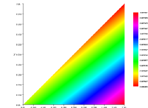
Figure 4: Numerical solution of the kernel component $k_{1}$ on $\mathbb{T}$

In Figure 5 are depicted the behavior in time of the control $U(t)$ and the output measurement $y(t)$. Clearly, despite the initial amplitude of $U(t)$, this latter one decreases in time and vanishes after $t\geq 4\,s$. Let us remind that the implementation of $U(t)$ requires a full-state measurement. Moreover, likewise $U(t)$ the output measurement $y(t)$ shows the same trend with its amplitude decreasing in time and tending to zero after $t\geq 3s$ as can be seen in Figure 5(b).

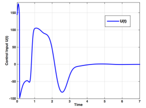
(a) Output control law

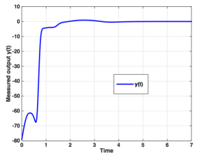
(b) Measured output

Figure 5: Evolution in time of the control law $U(t)$ and the measured output $y(t)$.

Plus, in figure (6) we plot the evolution in time of the $\mathcal{L}^{2}$-norm of the characteristics. As expected from the theoritical part we observe that the norm of the characteristics converge to zero. As a result this shows that the system (21) converge to the zero equilibrium. Thereby the physical linearized model (2 ) also converges to ($H^{*}$, $V^{*}$, $B^{*}$).

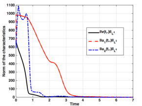
Figure 6: Evolution in time of the norm of the characteristic solution.

In addition, Figure 7 describes the space and time dynamics of the plant and is consistent with the numerical results presented above. As time increases, we notice that the perturbation in the overall system decreases and vanishes later.

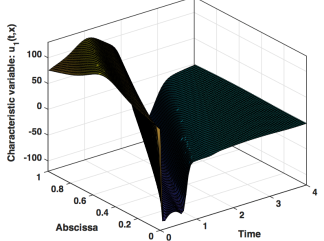
(a) Evolution of $u_{1}(t,x)$

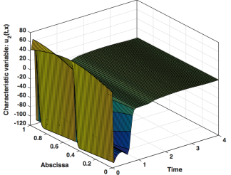
(b) Evolution of $u_{2}(t,x)$

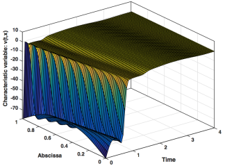
(c) Evolution of $v(t,x)$

Figure 7: Behavior in time and space of the characteristic solutions.

6.2 Output feedback under supercritical flow regime $(F_{r}>1)$

Here, all parameters of the physical model are listed in the following Table 2 given in the Appendix. In this subsection, the dynamic of the closed-loop system (19) together with the output feedback control law (88) is simulated The set point ($H^{*}$, $V^{*}$, $B^{*}$) leads to the following characteristic velocities

$$\lambda_{1}=1.87,\,\lambda_{2}=-0.74\text{ and }\lambda_{3}=8.13.$$

The Froude number is set to $Fr=1.6$. This test case is particularly challenging since the flow regime is supercritical. As previously we solve the kernel problem As previously the kernel problem (27)-(28) is solved numerically and the solution is used for the computation of the feedback control law (88). Not only that, the system (64)-(65) is also solved using the finite element setup and used to compute the kernel gain $p_{\rm i}(x)$ defined in $(\ref{gain-obs})$. This observer gain is represented in Figure 9.

In Figure (8) is depicted a snapshot of the numerical solution $k_{1}$ of the kernel PDEs (27)-(28) with the $x$ and $y$ coordinates defined as the horizontal and the vertical axis, respectively.

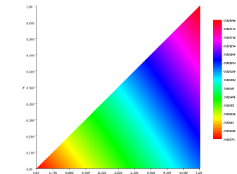
Figure 8: Solution component $k_{1}$ on the triangular domain $\mathbb{T}$.

The value of the kernel $k_{1}$, $k_{2}$ and $k_{3}$ at $x=1$ are the gain of the designed output feedback controller (88).

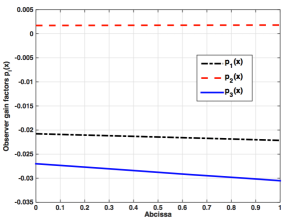
Figure 9: Computed observer gains $p_{\rm i}(x)$.

Elsewhere, the computation of the control law (88) requires also the knowledge of the observer. Then system (62)-(63) is solved on time and space. Figure 10 shows the evolution in time of the control input $U(t)$ at downstream and the output measurement $y(t)$ at upstream. Clearly, the amplitude of $U(t)$ decreases in time and vanishes for $t\geq 4\,s$.

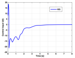
(a) Output control law

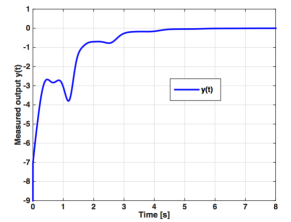
(b) Measured output

Figure 10: Evolution in time of the control law and the measured output

Moreover, the output measurement $y(t)$ shows the same trend with its amplitude decreasing in time and tends to zero after $t\geq 3$.
The dynamic of the $\mathcal{L}^{2}$-norm is directly related to the magnitude of the propagation speeds $\lambda_{i}$ as illustrated in Figure 11. Furthermore, we give a comparison of our output feedback law (Figure 11(a)) to the approach in [11] (Figure 11(b)) under this supercritical flow regime (fast rapid flow) where the conditions of Theorem 2 (cf [11]) are not fulfilled. Altogether, our approach exhibits a successful stabilization of system (19) around the zero equilibrium while instabilities are noticed when using the strategy presented in [11].

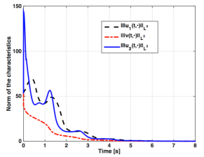
(a) Ouput feedback control through the backstepping design.

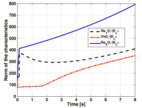
(b) Lyapunov design when the requirements of Theorem $2$ in [11] are not fulfilled.

Figure 11: Evolution in time of the norm of the characteristic solution.

Figure 12 describes the space and time dynamics of the plant and is consistent with the numerical results presented above. As time increases, we notice that the perturbation in the overall system decreases and vanishes later.

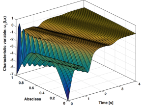
(a) Evolution of $u_{1}(t,x)$

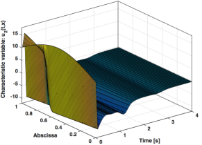
(b) Evolution of $u_{2}(t,x)$

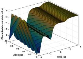
(c) Evolution of $v(t,x)$

Figure 12: Behavior in time and space of the distributed states.

As can be seen from these numerical simulations, the system (19) subject to the feedback control $U(t)$ is stabilized around the zero equilibrium as expected from the theoretical part. We clearly observed the expected qualitative and physical behavior of the designed control regardless the nature of the flow.
This class of state feedback law and output feedback controller we apply here allows to stabilize the SVE system in a optimal time when comparing with the results presented in [12] where a boundary measurement scenario is adopted.

7 Conclusion and future work

In this paper, a linearized Saint-Venant Exner model is analyzed for control purposes. The model describes the evolution of the water flow coupled with the transport of a sediment layer in an open channel. A backstepping state feedback controller, located at the downstream gate of the channel, is first designed for the (exponential) stabilization of the water level and the bathymetry at a desired equilibrium set, under the subcritical or supercritical flow regime. Then, based on an exponentially convergent Luenberger observer that reconstructs the full state, we design a a backstepping output feedback controller with the measurements at upstream. This controller also achieves the exponential stability of the linearized SVE model, for both subcritical and supercritical flow regime. Although the backstepping approach offers a more complicated design than the method developed in [11], it enables the exponential stabilization of the SVE system without any restriction on the system and the nature of the flow. It also reduces the number of actuators of the system: we only need a single boundary control in this paper, but on-line measurements of the water levels at both ends of the spatial domain are needed in [11]. Moreover, simulation results in comparison to [11] are provided to verify that the proposed controller moves beyond those limitations of [11].

We emphasize that practically, such systems are subjected to several types of perturbations and model uncertainties. Thus, an effective control action must take into account of these factors. We refer the readers to the recent results proposed in [28, 27] on the stabilization of hyperbolic PDEs with matched disturbances at the boundary input. In these papers, the authors employ sliding mode control and active disturbance rejection control to deal with them. Our future objective is to consider robustness issues for this application. Also, the extension of this approach to a network of flow and sediment transportation remains an interesting open problem with a high potential in real applications. Among the others, the problem of proving local stability of the nonlinear SVE plant under the linear feedback will be very interested to study.

Appendix

• Subcritical flow regime state feedback

  $T$	$\Delta x$	$CFL$	$A$	$p$	$C_{f}$	$\rho_{1}$	$\rho_{2}$
  8	0.01	0.95	0.008	0.002	0.1	1.5	1.5

  $q_{1}$	$q_{2}$	$H^{*}$	$U^{*}$	$B^{*}$
  1	1.2	2	3	0.4

  Table 1: Physical parameters and dimensionless numbers

• Supercritical flow regime output feedback

  $T$	$\Delta x$	$CFL$	$A_{g}$	$p_{g}$	$C_{f}$	$\rho_{1}$	$\rho_{2}$
  8	0.01	0.9	0.003	0.002	0.1	1	1.5

  $q_{1}$	$q_{2}$	$H^{*}$	$U^{*}$	$B^{*}$
  1	1.2	1	5	0.4

  Table 2: Physical parameters and dimensionless numbers

References

- [1] O. S. Balogun, M. Hubbard, and J. J. DeVries. Automatic control of canal flow using linear quadratic regulator theory. Journal of Hydraulic Engineering, 114(1):75–102, 1988.
- [2] P. Bernard and M. Krstic. Adaptive output-feedback stabilization of non-local hyperbolic PDEs. Automatica, 50(10):2692 – 2699, 2014.
- [3] J-M. Coron. Control and nonlinearity, volume 136 of Mathematical Surveys and Monographs. American Mathematical Society, Providence, RI, 2007.
- [4] J-M. Coron, G. Bastin, and B. d’Andréa Novel. Dissipative boundary conditions for one-dimensional nonlinear hyperbolic systems. SIAM J. Control Optim., 47(3):1460–1498, 2008.
- [5] J-M. Coron, B. d’Andréa Novel, and G. Bastin. A strict Lyapunov function for boundary control of hyperbolic systems of conservation laws. IEEE Trans. Automat. Control, 52(1):2–11, 2007.
- [6] J.-M. Coron, B. d’Andréa Novel, and G. Bastin. A Lyapunov approach to control irrigation canals modeled by saint venant equations. Proc. Eur. Control Conf., Karlsruhe, Germany, Sep. 1999.
- [7] J-M. Coron and Z. Q. Wang. Output feedback stabilization for a scalar conservation law with a nonlocal velocity. SIAM J. Math. Analysis, 45(5):2646–2665, 2013.
- [8] Jean-Michel Coron, Rafael Vazquez, Miroslav Krstic, and Georges Bastin. Local exponential H2 stabilization of a 22 quasilinear hyperbolic system using backstepping. SIAM Journal on Control and Optimization, 51(3):2005–2035, 2013.
- [9] F. Di Meglio, R. Vazquez, and M. Krstic. Stabilization of a system of coupled first-order hyperbolic linear PDEs with a single boundary input. IEEE Transactions on Automatic Control, 58(12):3097–3111, 2013.
- [10] Ben Mansour Dia and Jesper Oppelstrup. Boundary feedback control of 2-D shallow water equations. International Journal of Dynamics and Control, 1(1):41–53, March 2013.
- [11] Ababacar Diagne, Georges Bastin, and Jean-Michel Coron. Lyapunov exponential stability of 1-D linear hyperbolic systems of balance laws. Automatica, 48(1):109–114, 2011.
- [12] Ababacar Diagne and Abdou Sène. Control of shallow water and sediment continuity coupled system. Mathematics of Control, Signal and Systems (MCSS), pages 387–406, 2013.
- [13] M. Diagne, V. Dos Santos Martins, and M. Rodrigues. Une approche multi-modèles des équations de saint-venant : une analyse de la stabilité par techniques lmi. In Proceedings of Sixième Conférence Internationale Francophone d’Automatique, CIFA, NANCY, 2010.
- [14] V. Dos Santos, G. Bastin, J. M. Coron, and B. d’Andréa Novel. Boundary control with integral action for hyperbolic systems of conservation laws: Stability and experiments. Automatica, 44(5):1310–1318, 2008.
- [15] Mouhamadou Samsidy Goudiaby, Abdou Sène, and Gunilla Kreiss. A delayed feedback control for network of open canals. International Journal of Dynamics and Control, 1(4):316–329, December 2013.
- [16] J. M. Greenberg and Tatsien Li. The effect of boundary damping for the quasilinear wave equation. J. Differential Equations, 52(1):66–75, 1984.
- [17] J. Hudson and P.K. Sweby. Formulations for numerically approximating hyperbolic systems governing sediment transport. Journal of Scientific Computing, 19:225–252, 2003.
- [18] Miroslav Krstic and Andrey Smyshlyaev. Boundary control of PDEs: A course on backstepping designs, volume 16. Siam, 2008.
- [19] T.-T. Li. Global classical solutions for quasilinear hyperbolic systems. Research in Applied Mathematics. Masson and Viley, Berlin, 1994.
- [20] X. Litrico and Vincent Fromion. H∞ control of an irrigation canal pool with a mixed control politics. IEEE Transactions on Control Systems Technology, 14(1):99–111, 2006.
- [21] P. Malaterre. Pilote: Linear quadratic optimal controller for irrigation canals. Journal of Irrigation and Drainage Engineering, 124(4):187–194, 1998.
- [22] Pierre olivier Malaterre, David C. Rogers, and Jan Schuurmans. Classification of canal control algorithms. Journal of Irrigation and Drainage Engineering, 124(1):3–10, 1998.
- [23] P. Pognant-Gros, V. Fromion, and J.P. Baume. Canal controller design : a multivariable approach using h infini. In Proceedings of the European Control Conference, Portugal, pages 3398–3403, 2001.
- [24] Christophe Prieur and Jonathan de Halleux. Stabilization of a 1-D tank containing a fluid modeled by the shallow water equations. Systems & Control Letters, 52(3-4):167–178, 2004.
- [25] V. M. Dos Santos, M. Rodrigues, and M. Diagne. A multi-models approach of saint-venants equations : A stability study by lmi. International Journal of Applied Mathematics and Computer Science, 22(3):539–550, 2008.
- [26] A. Smyshlyaev and M. Krstic. Closed-form boundary state feedbacks for a class of 1-D partial integro-differential equations. Automatic Control, IEEE Transactions on, 49(12):2185–2202, Dec 2004.
- [27] S. Tang, B.-Z. Guo, and M. Krstic. Active disturbance rejection control for 22 hyperbolic systems with input disturbance. In IFAC World Congress, pages 1027–1032, 2014.
- [28] Shuxia Tang and Miroslav Krstic. Sliding mode control to the stabilization of a linear 2 2 hyperbolic system with boundary input disturbance. In American Control Conference (ACC), pages 1027–1032. IEEE, 2014.
- [29] Ying Tang, Christophe Prieur, and Antoine Girard. Boundary control synthesis for hyperbolic systems: a singular perturbation approach. In IEEE Conference on Decision and Control, Los Angeles, California, USA, 2014.
- [30] A. Tchousso, T. Besson, and C-Z. Xu. Exponential stability of distributed parameter systems governed by symmetric hyperbolic partial differential equations using Lyapunov’s second method. ESAIM Control Optim. Calc. Var., 15(2):403–425, 2009.
- [31] E. Weyer. LQ control of an irrigation channel. In Proceedings of the 42nd IEEE Conference on Decision and Control, volume 1, pages 750–755, 2003.
- [32] C. Z. Xu and G. Sallet. Proportional and integral regulation of irrigation canal systems governed by the saint-venant equation. In In Proceedings of the 14th world congress IFAC,Beijing, pages 147–152, 1999.
- [33] C. Z. Xu and G. Sallet. Exponential stability and transfer functions of processes governed by symmetric hyperbolic systems. ESAIM Control Optim. Calc. Var., 7:421–442 (electronic), 2002.