Polynomially Low Error PCPs with polyloglog n Queries via Modular Composition

We show that every language in NP has a PCP verifier that tosses $O(\log n)$ random coins, has perfect completeness, and a soundness error of at most $1/\text{poly}(n)$, while making at most $O(\text{poly}\log\log n)$ queries into a proof over an alphabet of size at most $n^{1/\text{poly}\log\log n}$. Previous constructions that obtain $1/\text{poly}(n)$ soundness error used either $\text{poly}\log n$ queries or an exponential sized alphabet, i.e. of size $2^{n^{c}}$ for some $c>0$. Our result is an exponential improvement in both parameters simultaneously.

Our result can be phrased as a polynomial-gap hardness for approximate CSPs with arity $\text{poly}\log\log n$ and alphabet size $n^{1/\text{poly}\log n}$. The ultimate goal, in this direction, would be to prove polynomial hardness for CSPs with constant arity and polynomial alphabet size (aka the sliding scale conjecture for inverse polynomial soundness error).

Our construction is based on a modular generalization of previous PCP constructions in this parameter regime,which involves a composition theorem that uses an extra ‘consistency’ query but maintains the inverse polynomial relation between the soundness error and the alphabet size.

Our main technical/conceptual contribution is a new notion of soundness, which we refer to as distributional soundness, that replaces the previous notion of “list decoding soundness”, and that allows us to prove a modular composition theorem with tighter parameters. This new notion of soundness allows us to invoke composition a super-constant number of times without incurring a blow-up in the soundness error.

1 Introduction

Probabilistically checkable proofs (PCPs) provide a proof format that enables verification with only a small number of queries into the proof such that the verification, though probabilistic, has only a small probability of error. This is formally captured by the following notion of a probabilistic verifier.

Definition 1.1 (PCP Verifier).

A PCP verifier $V$ for a language $L$ is a polynomial time probabilistic algorithm that behaves as follows: On input $x$, and oracle access to a (proof) string $\Pi$ (over an alphabet $\Sigma$), the verifier reads the input $x$, tosses some random coins $R$, and based on $x$ and $R$ computes a (local) window $I=(i_{\_}1,\ldots,i_{\_}q)$ of $q$ indices to read from $\Pi$, and a (local) predicate $\varphi:\Sigma^{q}\to\{0,1\}$. The verifier then accepts iff $\varphi(\Pi|_{\_}I)=1$.

• The verifier has perfect completeness: if for every $x\in L$, there is a proof $\Pi$ that is accepted with probability $1$. I.e., $\exists\Pi,\;\Pr_{\_}{R}[\varphi(\Pi|_{\_}I)=1]=1$.

• The verifier has soundness error $\delta<1$: if for any $x\not\in L$, every proof $\Pi$ is accepted with probability at most $\delta$. I.e., $\forall\Pi,\;\Pr_{\_}{R}[\varphi(\Pi|_{\_}I)=1]\leq\delta$.

The celebrated PCP Theorem [AS98, ALM⁺98] states that every language in NP has a verifier that has perfect completeness and soundness error bounded by a constant $\delta<1$, while using only a logarithmic number of random coins, and reading only $q=O(1)$ proof bits. Naturally (and motivated by the fruitful connection to inapproximability due to Feige et al. [FGL⁺96]), much attention has been given to obtaining PCPs with desirable parameters, such as a small number of queries $q$, smallest possible soundness error $\delta$, and smallest possible alphabet size $\left|\Sigma\right|$.

How small can we expect the soundness error $\delta$ to be? There are a couple of obvious limitations. First observe that the soundness error $\delta$ cannot be smaller than $1/\text{poly}(n)$ just because there are only $\text{poly}(n)$ different random choices for the verifier and at least one of the corresponding local predicates must be satisfiable. Next, note that if the verifier reads a total of ${k}$ bits from the proof (namely, $q\log\left|\Sigma\right|\leq{k}$), the soundness error cannot be smaller than $2^{-k}$, just because a random proof is expected to cause the verifier to accept with at least this probability.

The best case scenario is thus if one can have the verifier read ${k}=O(\log n)$ bits from the proof and achieve a soundness error of $1/2^{k}=1/\text{poly}(n)$. Indeed, the following is well known (obtained by applying a randomness efficient sequential repetition to the basic PCP Theorem):

Theorem 1.2 (PCP theorem + randomness efficient sequential repetition).

For every integer $k$, every language in NP has a PCP verifier that tosses at most $O(k+\log n)$ random coins, makes $q=O({k})$ queries into a proof over the Boolean alphabet $\{0,1\}$, has perfect completeness, and soundness error $\delta=2^{-{k}}$.

In particular, setting ${k}=\log n$ we get $q=O(\log n)$ and $\delta=1/\text{poly}(n)$.

This theorem gives a ballpark optimal tradeoff (up to constants) between soundness error and the number of bits read from the proof. However it does not achieve a small number of queries, a fundamental requirement that is important, among other things, for hardness of approximation. The goal of constructing a PCP with both a small error and a small number of queries turns out to be much more challenging and has attracted considerable attention. This was first formulated by Bellare et al. [BGLR93] as the “sliding scale” conjecture.

Conjecture 1.3 (Sliding Scale Conjecture [BGLR93]).

For any $\frac{1}{\text{poly}(n)}\leq\delta<1$, every language in NP has a PCP verifier that tosses $O(\log n)$ random coins, makes $q=O(1)$ queries into a proof over an alphabet $\Sigma$ of size $\text{poly}(1/\delta)$, has perfect completeness, and soundness error $\delta$.

As we describe shortly below, this conjecture is known to hold for $1>\delta\geq 2^{-(\log n)^{1-\varepsilon}}$, namely where $\delta$ can be made ‘almost’ polynomially small. The interesting regime, that has remained open for two decades, is that of (inverse) polynomially small $\delta$. This is the focus of our work. Our main goal is to find the smallest $q$ and $\left|\Sigma\right|$ parameters for which we can get $\delta$ to be polynomially small. Our main result is the following.

Main Theorem 1.4.

Every language in NP has a PCP verifier that tosses $O(\log n)$ random bits, makes $q=(\log\log n)^{O(1)}$ queries into a proof over an alphabet $\Sigma$ of size $\left|\Sigma\right|=n^{1/{(\log\log n)}^{O(1)}}$, has perfect completeness, and soundness error $\delta=1/\text{poly}(n)$.

Previous PCP constructions require at least $(\log n)^{\Omega(1)}$ queries in order to achieve polynomially small error (and this remains true even for constructions that are allowed quasi-polynomial size, see further discussion at the end of this introduction).

The first works making progress towards this conjecture are due to Raz and Safra [RS97], and Arora and Sudan [AS03], and rely on the classical (algebraic) constructions of PCPs. They prove the conjecture for all $\delta$ such that $\delta\geq 2^{-(\log n)^{\beta}}$ for some constant $\beta>0$. These ideas were then extended by Dinur et al. [DFK⁺11] with an elaborate composition-recursion structure, proving the conjecture for all $\delta\geq 2^{-(\log n)^{1-\varepsilon}}$ for any $\varepsilon>0$. The small catch here is that the number of queries grows as $\varepsilon$ approaches $0$. The exact dependence of $q$ on $\varepsilon$ was not explicitly analyzed in [DFK⁺11], but we show that it can be made $O(1/\varepsilon)$ while re-deriving their result.

Theorem 1.5 ([DFK⁺11]).

For every $\varepsilon>0$ and $\delta=2^{-(\log n)^{1-\varepsilon}}$, every language in NP has a PCP verifier that tosses $O(\log n)$ random coins, makes $q=O(1/\varepsilon)$ queries into a proof over an alphabet $\Sigma$ of size $\left|\Sigma\right|=1/\text{poly}(\delta)$, has perfect completeness, and has soundness error $\delta$.

The focus of [DFK⁺11] was on a constant number of queries but their result can also be applied towards getting polynomially small error with a non-trivially small number of queries. This is done by combining it with sequential repetition. We get,

Corollary 1.6 ([DFK⁺11] + randomness efficient sequential repetition).

For every $\varepsilon>0$, every language in NP has a PCP verifier that tosses $O(\log n)$ random coins, makes $q=O((\log n)^{\varepsilon}/\varepsilon)$ queries into a proof over an alphabet $\Sigma$ of size $\left|\Sigma\right|=2^{(\log n)^{1-\varepsilon}}$, has perfect completeness, and has soundness error $\delta=1/\text{poly}(n)$.

Corollary 1.6 describes the previously known best result in terms of minimizing the number of queries subject to achieving a polynomially small error and using at most a logarithmic amount of randomness. Whereas in Corollary 1.6 the number of queries is $q=(\log n)^{\varepsilon}$, our Main Theorem 1.7 requires only $q=\text{poly}\log\log n$ queries.

PCP Composition and dPCPs

Like in recent improved constructions of PCPs [BGH⁺06, DR06, BS08, Din07, MR10, DH13], our main theorem is obtained via a better understanding of composition. All known constructions of PCPs rely on proof composition. This paradigm, introduced by Arora and Safra [AS98], is a recursive procedure applied to PCP constructions to reduce the alphabet size. The idea is to start with an easier task of constructing a PCP over a very large alphabet $\Sigma$. Then, proof composition is applied (possibly several times over) to PCPs over the large alphabet to obtain PCPs over a smaller (even binary) alphabet, while keeping the soundness error small.

In the regime of high soundness error (greater than 1/2), composition is by now well understood using the notion of PCPs of proximity [BGH⁺06] (called assignment testers in [DR06]) (see also [Sze99]). The idea is to bind the PCP proof of a statement to an NP witness for it, so that the verifier not only checks that the statement is correct but also that the given witness is (close to) a valid one. This extension allows one to prove a modular composition theorem, which is oblivious to the inner makings of the PCPs being composed. This modular approach has facilitated alternate proofs of the PCP theorem and constructions of shorter PCPs [BGH⁺06, BS08, Din07]. However, the notion of a PCP of proximity, or assignment tester, is not useful for PCPs with low-soundness error. The reason is that for small $\delta$ we are in a “list decoding regime”, in that the PCP proof can be simultaneously correlated with more than one valid NP witness.

The works mentioned earlier [RS97, AS03, DFK⁺11] addressed this issue by using a notion of local list-decoding. This was called a local-reader in [DFK⁺11] and formalized nicely as a locally-decode-or-reject-code (LDRC) by Moshkovitz and Raz [MR10]. Such a code allows “local decoding” in that for any given string $w$ there is a list of valid codewords $\left\{c_{\_}1,\ldots,c_{\_}L\right\}$ such that when the verifier is given a tuple of indices $j_{\_}1,\ldots,j_{\_}k$, then but for an error probability of $\delta$, the verifier either rejects or outputs $(c_{\_}i)|_{\_}{j_{\_}1,\ldots,j_{\_}k}$ for some $i\in[L]$.

Decodable PCPs (dPCPs)

Dinur and Harsha [DH13] introduced the notion of a PCP decoder (dPCP), which extends the earlier definitions of LDRCs and local-readers from codes to PCP verifiers. A PCP decoder is like a PCP verifier except that it also gets as input an index $j$ (or a tuple of indices). The PCP decoder is supposed to check that the proof is correct, and to also return the $j$-th symbol of the NP witness encoded by the PCP proof. As in previous work, the soundness guarantee for dPCPs is that for any given proof $\Pi$ there is a short list of valid NP witnesses $\left\{x_{\_}1,\ldots,x_{\_}L\right\}$ such that except with probability $\delta$ the verifier either rejects or outputs $(x_{\_}i)|_{\_}j$ for some $x_{\_}i$ in the list.

The main advantage of dPCPs is that they allow a modular composition theorem in the regime of small soundness error. The composition theorem proved by Dinur and Harsha [DH13] was a two-query composition theorem, generalizing from the ingenious construction of Moshkovitz and Raz [MR10]. The two-query requirement is a stringent one, and in this construction it inherently causes an exponential increase in the alphabet, so that instead of $\left|\Sigma\right|=\text{poly}(1/\delta)$ one gets a PCP with $\left|\Sigma\right|=\exp(\text{poly}(1/\delta))$.

In this work we give a different (modular) dPCP composition theorem. Essentially, our theorem is a modular generalization of the composition method, as done implicitly in previous works [RS97, AS03, DFK⁺11], which uses an extra ‘consistency’ query but maintains the inverse polynomial relation between $\delta$ and $\left|\Sigma\right|$.

We remark that unlike recent PCP constructions [BGH⁺06, DR06, MR10, DH13] which recurse on the large (projection) query of the outer PCP, our composition recurses on the entire test as was done originally by Arora and Safra [AS98]. This aspect of the composition is explained and abstracted nicely in [Mos14].

Distributional Soundness

Our main technical/conceptual contribution is a new notion of soundness, which we refer to as distributional soundness, which replaces the previous notion of list decoding soundness described above, and allows us to apply a non-constant number of compositions without a blowup in the error.

We say that a verifier has distributional soundness $\delta$ if its output is “$\delta$-indistinguishable” from the output of an idealized verifier. The idealized verifier has access to a distribution $\widetilde{\Pi}$ over valid proofs or $\bot$. When it is run with random coins $R$ it samples a proof $\widetilde{\Pi}(R)$ from this distribution and either rejects if $\widetilde{\Pi}(R)=\bot$ or outputs what the actual verifier would output when given access to $\widetilde{\Pi}(R)$. By $\delta$-indistinguishable, we mean that there is a coupling between the actual verifier and the idealized verifier, such that the probability that the verifier does not reject and its output differs from the output of the idealized verifier, is at most $\delta$.

The advantage of moving from list decoding soundness to distributional soundness, is that it removes the extra factor of $L_{\_}{\mathrm{in}}$ (the list size) incurred in previous composition analyses. Recall that, e.g. in the composition theorem of Dinur-Harsha [DH13], one takes an outer PCP with soundness $\delta_{\mathrm{out}}$ and an inner PCP decoder with soundness $\delta_{\mathrm{in}}$ and out comes a PCP with soundness $\delta_{\mathrm{in}}+L_{\_}{\mathrm{in}}\cdot\delta_{\mathrm{out}}$. This is true in all (including implicit) prior composition analyses. When making only a constant number of composition steps, this is not an issue, but when the number $t$ of composition steps grows, the soundness is at least $(L_{\_}{\mathrm{in}})^{t}\cdot\delta_{\mathrm{out}}$ and this is too expensive for the parameters we seek. Using distributional soundness, we prove that the composition of a PCP with soundness error $\delta_{\mathrm{out}}$ and a dPCP with soundness error $\delta_{\mathrm{in}}$ yields a PCP with soundness error $\delta_{\mathrm{out}}+\delta_{\mathrm{in}}+\eta$ where $\eta$ is an error term that is related to the distance of an underlying error correcting code, and can be controlled easily. Thus, after $t$ composition steps the soundness error will only be $O(t(\delta+\eta))$.

We remark that this notion of soundness, though new, is satisfied by most of the earlier PCP constructions (at least the ones based on the low-degree test). In particular, it can be shown that list-decoding soundness and very good error-correcting properties of the PCP imply distributional soundness.

Proof Overview

At a high level, our main theorem is derived by adopting the recursive structure of the construction in [DFK⁺11]. The two main differences are the use of our modular composition theorem, and the soundness analysis that relies on the notion of distributional soundness.

We fix a field $\mathbb{F}$ at the outset and use the same field throughout the construction. This is important for the interface between the outer and the inner dPCPs, as it provides a convenient representation of the output of the outer dPCP as an arithmetic circuit over $\mathbb{F}$, which is then the input for the inner dPCP.

As in the construction of [DFK⁺11], we take $\left|\mathbb{F}\right|\approx 2^{(\log n)^{1-\varepsilon}}$ and begin by constructing PCPs over a fairly large alphabet size which we gradually reduce via composition. The initial alphabet size is $2^{2^{(\log n)^{1-\varepsilon}}}$, and then it drops to $2^{2^{(\log n)^{1-{\bf 2}\varepsilon}}}$ and then to $2^{2^{(\log n)^{1-{\bf 3}\varepsilon}}}$ and so on. After $1/\varepsilon$ steps we make a couple of final composition steps and end up with the desired alphabet size of $2^{(\log n)^{1-\varepsilon}}$, logarithmic in the initial alphabet size.

Unlike the construction in [DFK⁺11], we can afford to plug in a sub-constant value for $\varepsilon$, and we take $\varepsilon=c\log\log\log n/\log\log n$ for some constant $c$ so that $2^{(\log n)^{1-\varepsilon}}=2^{\log n/(\log\log n)^{c}}=n^{1/(\log\log n)^{c}}$.

The number of composition steps is $O(1/\varepsilon)$, resulting in a PCP with $O(\log\log n)$ queries and soundness error $n^{1/(\log\log n)^{c}}$ for some constant $c<3$ (see Theorem 5.1). Finally, $(\log\log n)^{c}$ steps of (randomness-efficient) sequential repetition yield a PCP with polynomially small error and $\text{poly}\log\log n$ queries as stated in Main Theorem 1.7. It can be shown that the parameters obtained in Theorem 5.1 (namely, soundness error $n^{1/(\log\log n)^{O(1)}}$) is tight given the basic Reed-Muller and Hadamard based building blocks (see § 5.3 for details).

Further Background and Motivation

Every PCP theorem can be viewed as a statement about the local-vs.-global behaviour of proofs, in that the correctness of a proof, which is clearly a global property, can be checked by local checks, on average. The parameters of the PCP (number of queries, soundness error, alphabet size) give a quantitative measure to this local to global behavior. The sliding scale conjecture essentially says that even with a constant number of queries, this local to global phenomenon continues to hold, for all ranges of the soundness error.

Another motivation for minimizing the number of queries becomes apparent when considering interaction with provers instead of direct access to proofs (i.e. MIP instead of PCP). A PCP protocol can not in general be simulated by a protocol between a verifier and a prover because the prover might cheat by adaptively changing her answers. This can be sidestepped by sending each query to a different prover, such that the provers are not allowed to communicate with each other. This is the MIP model of Ben-Or et al. [BGKW88]. It is only natural to seek protocols using the smallest number of (non-communicating) provers.

The importance of the sliding scale conjecture stems, in addition to the fundamental nature of the question, from its applications to hardness of approximation. First, it is known that every PCP theorem can be phrased as a hardness-of-approximation for Max-CSP: the problem of finding an assignment that satisfies a maximal number of constraints in a given constraint system. The soundness error translates to the approximation factor, the alphabet of the proof is the alphabet of the variables, and the number of queries becomes the arity of the constraints in the CSP.

The main goal of this paper can be phrased as proving polynomial hardness of approximation factors for CSPs with smallest possible arity (and over an appropriately small alphabet). Our main theorem translates to the following result

Theorem 1.7.

It is NP-hard to decide if a given CSP with $n$ variables and $\text{poly}(n)$ constraints, is perfectly satisfiable or whether every assignment satisfies at most $1/\text{poly}(n)$ fraction of the constraints. The CSP is such that each constraint has arity at most $\text{poly}\log\log n$ and the variables take values over an alphabet of size at most $n^{1/\log\log n^{O(1)}}$.

In addition to the syntactic connection to Max-CSP, it is also known that a proof of the sliding scale conjecture would immediately imply polynomial factors inapproximability for Directed-Sparsest-Cut and Directed-Multi-Cut [CK09].

The results of [DFK⁺11] were used in [DS04] for proving hardness of approximation for a certain $\ell_{\_}p$ variant of label cover. However, that work mis-quoted the main result from [DFK⁺11] as holding true even for a super-constant number of queries, up to $\sqrt{\log\log n}$. In this work, we fill the gap proving the required PCP statement. We thank Michael Elkin for pointing this out.

Further Discussion

A possible alternate route to small soundness PCPs is via the combination of the basic PCP theorem [AS98, ALM⁺98] with the parallel repetition theorem [Raz98]. Applying $k$-fold parallel repetition yields a two-query PCP verifier over alphabet of size $\left|\Sigma\right|=2^{O(k)}$, that uses $O(k\log n)$ random bits, and has soundness error $\delta=2^{-\Omega(k)}$.

If we restrict to polynomial-size constructions, then parallel repetition is of no help compared to Theorem 1.2. If we allow $k$ to be super constant, then more can be obtained. First, it is important to realize that the soundness error should be measured in terms of the output size, namely $N=2^{k\log n}$. For $k=(\log n)^{c}$ a simple calculation shows $\log n=(\log N)^{1/(c+1)}$, and hence the soundness error is $\delta(N)=2^{-(\log n)^{c}}=2^{-(\log N)^{1-1/(c+1)}}$. This is no better than the result of [DFK⁺11] in terms of the soundness error, and in fact, worse in terms of the instance size blow up ($N=2^{(\log n)^{c+1}}$ as opposed to $N=n^{O(1)}$). Even parameters similar to our main theorem can be obtained, albeit with an almost exponential blowup. Consider $k=\sqrt{n}$ for example. In this case $\log n=2\log\log N-\Theta(\log\log\log N)$, and so $\delta(N)=2^{-\sqrt{n}}=N^{-1/\Theta(\log\log N)}$. From here, to get a polynomially small error one can take $O(\log\log N)$ rounds of (randomness efficient) sequential repetition, coming up with a result that is similar to our Main Theorem 1.7 but with a huge blow up $(N=n^{\sqrt{n}}$ as opposed to $N=n^{O(1)}$).

We remark that a natural approach towards the sliding scale conjecture is to try and find a randomness-efficient version of parallel repetition to match the parameters of Theorem 1.2 but with $q=O(1)$. Unfortunately, this approach has serious limitations [FK95] and has so-far been less successful than the algebra-and-composition route, see also [DM11, Mos14].

Organization

We begin with some preliminaries in § 2. We introduce and define dPCPs and distributional soundness in § 3. Our dPCPs have $k$ provers which are analogous to (and stronger than) PCPs that make $k$ queries. In § 4, we state and prove a modular composition theorem for two (algebraic) dPCPs. In § 5, we prove the main theorem, relying on specific “classical” constructions of PCPs that are given in § 6, one based on the Reed-Muller code and low degree test, and one based on the quadratic version of the Hadamard code. These PCPs are the same as in earlier constructs [RS97, AS03, DFK⁺11, MR10, DH13] except that here we prove that they have the stronger notion of small distributional soundness.

2 Preliminaries

2.1 Notation

All circuits in this paper have fan-in 2 and fan-out 2, and we allow only unary NOT and binary AND Boolean operations as internal gates. The size of a Boolean circuit/predicate $\Phi$ is the number of gates in $\Phi$. Given a circuit/predicate $\Phi:\left\{0,1\right\}^{n}\to\left\{0,1\right\}$, we denote by $\mbox{{{SAT}}}(\Phi)$ the set of satisfying assignments for $\Phi$, i.e.,

$$\mbox{{{SAT}}}(\Phi)=\left\{x\in\left\{0,1\right\}^{n}\left|\;\vphantom{x\in\left\{0,1\right\}^{n}\Phi(x)=1}\right.\Phi(x)=1\right\}.$$

We will refer to the following NP-complete language associated with circuits:

$$\mbox{{{CktSAT}}}=\left\{\Phi\left|\;\vphantom{\Phi\Phi\text{ is specified as a Boolean circuit and }\mbox{{{SAT}}}(\Phi)\neq\emptyset}\right.\Phi\text{ is specified as a Boolean circuit and }\mbox{{{SAT}}}(\Phi)\neq\emptyset\right\}.$$

We will follow the following convention regarding input lengths: $n$ will refer to the length of the input to the circuit $\Phi$ (i.e., $\Phi:\left\{0,1\right\}^{n}\to\left\{0,1\right\}$) while $N$ will refer to the size of the circuit/predicate (i.e., $\text{size}(\Phi)=N$). Thus, $N$ is the input size to the problem CktSAT.

We will also refer to a similar language associated with arithmetic circuits. First, for some notation. Given a finite field $\mathbb{F}$, we consider arithmetic circuits over $\mathbb{F}$ with addition ($+$) and multiplication ($\times$) gates and constants from the field $\mathbb{F}$. For a function $\Phi:\mathbb{F}^{n}\to\mathbb{F}$, the size of $\Phi$ is the number of gates in the arithmetic circuit specifying $\Phi$. We denote by $\mbox{{{SAT}}}(\Phi)$ the set of all $x$ such that $\Phi(x)=0$.

Definition 2.1 (Algebraic Circuit SAT).

Given a field $\mathbb{F}$, the Algebraic-Circuit-Satisfiability problem, denoted by $\mbox{{{Alg-CktSAT}}}_{\_}\mathbb{F}$, is defined as follows:

$$\mbox{{{Alg-CktSAT}}}_{\_}\mathbb{F}=\left\{\Phi\left|\;\vphantom{\Phi\Phi\text{ is specified by an arithmetic circuit over }\mathbb{F}\text{ and }\mbox{{{SAT}}}(\Phi)\neq\emptyset}\right.\Phi\text{ is specified by an arithmetic circuit over }\mathbb{F}\text{ and }\mbox{{{SAT}}}(\Phi)\neq\emptyset\right\}.$$

As in the case of CktSAT, $n$ refers to the length of the input to the function $\Phi$ (i.e., $\Phi:\mathbb{F}^{n}\to\mathbb{F}$), while $N$ refers to the size of the arithmetic circuit $\Phi$.

2.2 Error Correcting Codes

Let $E:\mathbb{F}^{n}\to\mathbb{F}^{N}$ be an error correcting code with relative distance $1-\mu$, i.e., for every $x\neq x^{\prime}$, $\Pr_{\_}{j\in[N]}[E(x)_{\_}j=E(x^{\prime})_{\_}j]\leq\mu$. For a word $w\in\mathbb{F}^{N}$ that is not necessarily a correct codeword, we can consider the list of all “admissible” codewords, i.e. codewords that have a non-negligible correlation with $w$. We are interested in more than just a list: we want to associate with each index $j\in[N]$ an element in that list in a unique way. This will allow us to treat $w$ as a random variable $W$: for a random index $j$, the random variable $W(j)$ will output the list-element associated with the $j$th index.

Definition 2.2.

Let $\tau>0$ be a parameter an let $w:[N]\to\mathbb{F}$. We define the $\tau$-local decoding function of $w$ with respect to the code $E$,  $W:[N]\to\mathbb{F}^{n}\cup\left\{\bot\right\}$, as follows:

• The $\tau$-admissible words for $w$ are

  $$agr_{\_}\tau(w)=\left\{x\in\mathbb{F}^{n}\left|\;\vphantom{x\in\mathbb{F}^{n}\Pr_{\_}{j\in[N]}[E(x)_{\_}j=w_{\_}j]\geq\tau}\right.\Pr_{\_}{j\in[N]}[E(x)_{\_}j=w_{\_}j]\geq\tau\right\}.$$

• For any $j\in[N]$, if there is a unique word $x\in\mathrm{agr}_{\_}\tau(w)$ such that $E(x)_{\_}j=w_{\_}j$ we set $W(j)=x$. Otherwise, we set $W(j)=\bot$.

Claim 2.3.

Let $E:\mathbb{F}^{n}\to\mathbb{F}^{N}$ be an error correcting code with relative distance $1-\mu$, let $w:[N]\to F$, and let $W:[N]\to\mathbb{F}^{n}$ be its $\tau$-local decoding function with respect to $E$. Also, suppose that $v:[N]\to\mathbb{F}$ is a legal codeword, i.e., $v=E(y)$ for some $y\in\mathbb{F}^{n}$. Then

$$\Pr_{\_}{j\in[N]}\left[v_{\_}j=w_{\_}j{\hbox{ and }}W(j)\neq y\right]\leq\tau+4\mu/\tau^{2}.$$

Proof.

Without loss of generality, we may assume that $\tau\geq 2\sqrt{\mu}$. Let us write $\mathrm{agr}_{\_}\tau(w)=\left\{x_{\_}1,x_{\_}2,\ldots\right\}$ and let $S_{\_}i=\left\{j\in[N]\left|\;\vphantom{j\in[N]w_{\_}j=(E(x_{\_}i))_{\_}j}\right.w_{\_}j=(E(x_{\_}i))_{\_}j\right\}$. We say that $j\in[N]$ is an ambiguous point for $w$ if $j\in S_{\_}i\cap S_{\_}{i^{\prime}}$ for some distinct $i,i^{\prime}$. We first bound the fraction of ambiguous points for $w$.

By inclusion-exclusion, for any $\ell\leq\left|\mathrm{agr}_{\_}\tau(w)\right|$

$$N\geq\left|\cup_{\_}{i=1}^{\ell}S_{\_}i\right|\geq\sum_{\_}{i=1}^{\ell}\left|S_{\_}i\right|-\sum_{\_}{i\neq{i^{\prime}}\leq\ell}\left|S_{\_}{i}\cap S_{\_}{i^{\prime}}\right|)\geq\ell\tau N-\binom{\ell}{2}\mu N,$$

where we have used that by definition $\left|S_{\_}i\right|\geq\tau N$ and by the distance of the code $\left|S_{\_}i\cap S_{\_}{i^{\prime}}\right|\leq\mu N$. This implies that for every $\ell\leq\left|\mathrm{agr}_{\_}\tau(w)\right|$,

$$1\geq\ell\tau-\binom{\ell}{2}\mu\geq\ell\tau-\ell^{2}\tau^{2}/8$$

which clearly fails if $\ell=2/\tau$, so $\left|\mathrm{agr}_{\_}\tau(w)\right|\leq 2/\tau$ and so

$$\Pr_{\_}{j\in[N]}[j\text{ is ambiguous}]\leq\frac{1}{N}\sum_{\_}{i\neq{i^{\prime}}}\left|S_{\_}i\cap S_{\_}{i^{\prime}}\right|\leq 4\mu/\tau^{2}$$ (2.1)

Now the event $\left[v_{\_}j=w_{\_}j{\hbox{ and }}W(j)\neq y\right]$ can occur either if $j$ is an ambiguous point for $w$, or if $v$ is not $\tau$-admissible with respect to $w$. But the former happens with probability at most $4\mu/\tau^{2}$ by (2.1), and the latter happens with probability at most $\tau$, as otherwise $v$ would have been $\tau$-admissible. ∎

Remark 2.4.

We minimize the quantity $\tau+4\mu/\tau^{2}$, by setting $\tau=(4\mu)^{1/3}$. We refer to this minimum as the agreement parameter $\eta$ of the code $E$. Thus, $\eta=2\tau=2(4\mu)^{1/3}$.

3 PCPs with distributional soundness

3.1 Standard PCPs

We begin by recalling the definition of a standard $k$-prover projection PCP verifier.

Definition 3.1 (PCP verifier).

• A $k$-prover projection PCP verifier over alphabet $\mathbb{F}$ is a probabilistic-time algorithm $V$ that on input $\Phi$, a circuit of size $N$ and a random input $R$ of $r(N)$ random bits generates a tuple $(q,\varphi,g)$ where $q=(u,v_{\_}1\dots,v_{\_}{k-1})$ is a vector of $k$ queries, $\varphi:\mathbb{F}^{m}\to\left\{0,1\right\}$ is a predicate, and $g=(g_{\_}1,\dots,g_{\_}{k-1})$ is a list of $k-1$ functions $g_{\_}i:\mathbb{F}^{m}\to\mathbb{F}$ such that the size of the tuple $(\varphi,g)$ is at most $s(N)$.

• We write $(q,\varphi,g)=V(\Phi;R)$ to denote the query-predicate-function tuple output by the verifier $V$ on input $\Phi$ and random input $R$.

• It is good to keep in mind the $k=2$ case as it captures all of the difficulty. In this case the output of $V$ is a label cover instance, when enumerating over all of $V$’s random inputs. (The query pairs specify edges $(u,v)$ and $(\varphi,g)$ specify which pairs of labels are acceptable).

• We think of $V$ as a probabilistic oracle machine that on input $(\Phi;R)$ queries $k$ provers $\Pi=(A,B_{\_}1,\dots,B_{\_}{k-1})$ at positions $q=(u,v_{\_}1,\dots,v_{\_}{k-1})$ respectively to receive the answers $\Pi|_{\_}q:=$ $(A(u),B_{\_}1(v_{\_}1),\dots,B_{\_}{k-1}(v_{\_}{k-1}))$ $\in\mathbb{F}^{m}\times\mathbb{F}^{k-1}$, and accepts iff the following checks pass: $\varphi(A(u))=1$ and $g_{\_}i(A(u))=B_{\_}i(v_{\_}i)$ for all $i\in\{1,\dots,k-1\}$.

• Given $k$ provers $\Pi=(A,B_{\_}1,\dots,B_{\_}{k-1})$, we will sometimes collectively refer to them as the “proof $\Pi$” . Furthermore, we refer to $A$ as the large prover and the $B_{\_}i$’s as the projection provers. We call $\Pi|_{\_}q$ the local view of the proof $\Pi$ on queries $q$ and denote by $V^{\Pi}(\Phi;R)$ the output of the verifier $V$ on input $(\Phi;R)$ when interacting with the $k$ provers $\Pi$. Thus, $V^{\Pi}(\Phi;R)=\mbox{{{acc}}}$ if the checks pass and is rej otherwise.

• We call $N$ the input size, $k$ the number of provers, $r(N)$ the randomness complexity, and $s(N)$ the answer size of the verifier $V$.

Definition 3.2 (standard PCPs).

For a function $\delta:\mathbb{Z}^{+}\to[0,1]$, a $k$-prover projection PCP verifier $V$ is a $k$-prover probabilistically checkable proof system for CktSAT with soundness error $\delta$ if the following completeness and soundness properties hold for every circuit $\Phi$:

Completeness:

If $x\in\mbox{{{SAT}}}(\Phi)$, then there exist $k$ provers $\Pi=(A,B_{\_}1,\dots,B_{\_}{k-1})$ that cause the verifier $V$ to accept with probability 1. Formally,

$$\exists\Pi=(A,B_{\_}1,\dots,B_{\_}{k-1}),\qquad\Pr_{\_}{R}\left[V^{\Pi}(\Phi;R)=\mbox{{{acc}}}\right]=1.$$

In this case, we say that $\Pi$ is a valid proof for the statement $x\in\mbox{{{SAT}}}(\Phi)$.

Soundness:

If $\Phi\notin\mbox{{{CktSAT}}}$ (i.e, $\mbox{{{SAT}}}(\Phi)=\emptyset$), then for every $k$ provers $\Pi=(A,B_{\_}1,\dots,B_{\_}{k-1})$, the verifier $V$ accepts $\Phi$ with probability at most $\delta(N)$. Formally,

$$\forall\Pi=(A,B_{\_}1,\dots,B_{\_}{k-1}),\qquad\Pr_{\_}{R}\left[V^{\Pi}(\Phi;R)=\mbox{{{acc}}}\right]\leq\delta(N).$$

We then say that CktSAT has a $k$-prover projective PCP with soundness error $\delta$.

3.2 Distributional Soundness

We now present distributional soundness, a strengthening of the standard PCP soundness condition that we find to be very natural. Informally, distributional soundness means that the event of the verifier accepting is roughly the same as the event of the local view of the verifier being consistent with a globally consistent proof, up to ”the soundness error”. I.e.,

$$\Pr[\hbox{ accept }]=\Pr[\hbox{ accept ~{}~{}and~{}~{} the local view agrees with a correct proof }]\pm\delta.$$

Thus, the local acceptance of the verifier is ”fully explained” in terms of global consistency.

A little more formally, every purported proof $\Pi$ (valid or not) can be coupled with an “idealized” distribution ${\widetilde{\Pi}}(R)$ over valid proofs and $\bot$ such that the behavior of the verifier on random string $R$ when interacting with the proof $\Pi$ is identical to the corresponding behavior when interacting with the “idealized” proof ${\widetilde{\Pi}}(R)$ upto an error of $\delta$, which we call the distributional soundness error. Formally,

Definition 3.3 (Distributional Soundness for $k$-prover PCPs).

For a function $\delta:\mathbb{Z}^{+}\to[0,1]$, a $k$-prover projection PCP verifier $V$ for CktSAT is said to have distributional soundness error $\delta$ if for every circuit $\Phi$ and any set of provers $\Pi=(A,B_{\_}1,\dots,B_{\_}{k-1})$ there is an ‘idealized pair’ of functions ${\widetilde{x}}(R)$ and ${\widetilde{\Pi}}(R)$ defined for every random string $R$ such that the following holds.

• For every random string $R$, ${\widetilde{\Pi}}(R)$ is either a valid proof for the statement ${\widetilde{x}}(R)\in SAT(\Phi)$, or ${\widetilde{\Pi}}(R)=\bot$.

• With probability at least $1-\delta$ over the choice of the random string $R$, the local view of the provers $\Pi$ completely agrees with the local view of the provers ${\widetilde{\Pi}}(R)$ or is a rejecting local view. In other words,

  $$\Pr_{\_}R\left[V^{\Pi}(\Phi;R)=\bot\text{ or }\Pi|_{\_}q={\widetilde{\Pi}}(R)|_{\_}q\right]\geq 1-\delta,$$

  where $q$ is the query vector generated by the PCP verifier $V$ on input $(\Phi;R)$.

  When the local views agree, i.e. $\Pi|_{\_}q={\widetilde{\Pi}}(R)|_{\_}q$, we say that ${\widetilde{\Pi}}$ is successful (in explaining the success of $\Pi$).

The advantage of distributional soundness is that it explains the acceptance probability of every proof $\Pi$, valid or otherwise, in the following sense. Suppose a proof $\Pi$ is accepted with probability $p$. I.e., $p$ fraction of the local views $\Pi|_{\_}q$ are “accepting”. Then, it must be the case that but for an error probability of $\delta$, each of these accepting views are projections of (possibly different) valid proofs. It is an easy consequence of this, that distributional soundness implies (standard) soundness.

Proposition 3.4.

If CSAT has a $k$-prover PCP with distributional soundness error $\delta$, then CktSAT has a $k$-prover PCP with (standard) soundness error $\delta$. Furthermore, all other parameters (randomness, answer size, alphabet, perfect completeness) are identical.

Proof.

Suppose there exists a circuit $\Phi$ and a proof $\Pi$ such that $\Pr_{\_}R\left[V^{\Pi}(\Phi;R)=\mbox{{{acc}}}\right]>\delta$. Then, by the distributional soundness property it follows that there exists at least one local accepting view which is a projection of a valid proof. In particular, there exists a valid proof which implies $\Phi\in\mbox{{{CktSAT}}}$. ∎

3.3 PCP decoders

We now present a variant of PCP verifiers, called PCP decoders, introduced by Dinur and Harsha [DH13]. PCP decoders, as the name suggests, have the additional property that they not only locally check the PCP proof $\Pi$, but can also locally decode symbols of an encoding of the original NP witness from the PCP proof $\Pi$. PCP decoders are implicit in many previous constructions of PCPs with small soundness error and were first explicitly defined under the name of local-readers by Dinur et al. [DFK⁺11], as locally-decode-or-reject-codes (LDRC) by Moshkovitz and Raz [MR10] and as decodable PCPs by Dinur and Harsha [DH13]. As in the case of PCP verifiers, our PCP decoders will be projection PCP decoders.

Definition 3.5 (PCP decoder).

• A $k$-prover $l$-answer projection PCP decoder over alphabet $\mathbb{F}$ and encoding length $t$ is a probabilistic-time algorithm $\mathcal{D}$ that on input $(\Phi,F)$ of size $N$, a random input string $R$ of $r(N)$ random bits and an additional input index $j\in[t]$, where $\Phi:\mathbb{F}^{n}\to\left\{0,1\right\}$ is a predicate, and $F=(F_{\_}1,\dots,F_{\_}{l-1})$ a list of $l-1$ functions $F_{\_}i:\mathbb{F}^{n}\to\mathbb{F}$, generates a tuple $(q,\varphi,g,f)$ where $q=(u,v_{\_}1\dots,v_{\_}{k-1})$ is a vector of $k$ queries, $\varphi:\mathbb{F}^{m}\to\left\{0,1\right\}$ is a predicate, $g=(g_{\_}1,\dots,g_{\_}{k-1})$ is a list of $k-1$ functions $g_{\_}i:\mathbb{F}^{m}\to\mathbb{F}$ and $f=(f_{\_}0,\dots,f_{\_}{l-1})$ is a list of $l$ functions $f_{\_}i:\mathbb{F}^{m}\to\mathbb{F}$ such that the size of the tuple $(\varphi,g,f)$ is at most $s(N)$.

• We write $(q,\varphi,g,f)=\mathcal{D}(\Phi,F;R,j)$ to denote the query-predicate-functions tuple output by the decoder $\mathcal{D}$ on input pair $(\Phi,F)$, random input $R$ and input index $j$.

• We think of $\mathcal{D}$ as a probabilistic oracle machine that on input $(\Phi,F;R,j)$ queries $k$ provers $\Pi=(A,B_{\_}1,\dots,B_{\_}{k-1})$ at positions $q=(u,v_{\_}1,\dots,v_{\_}{k-1})$ respectively to receive the answers $\Pi|_{\_}q:=$
  $(A(u),B_{\_}1(v_{\_}1),\dots,B_{\_}{k-1}(v_{\_}{k-1}))$ $\in\mathbb{F}^{m}\times\mathbb{F}^{k-1}$, then checks if $\varphi(A(u))=1$ and $g_{\_}i(A(u))=B_{\_}i(v_{\_}i)$ for all $i\in\{1,\dots,k-1\}$ and if these tests pass outputs the $l$-tuple $(f_{\_}0(A(u)),f_{\_}1(A(u)),\dots,f_{\_}{l-1}(A(u)))\in\mathbb{F}^{l+1}$ and otherwise outputs $\bot$.

• Given $k$ provers $\Pi=(A,B_{\_}1,\dots,B_{\_}{k-1})$, we will sometimes collectively refer to them as the “proof $\Pi$” . Furthermore, we refer to $A$ as the large prover and the $B_{\_}i$’s as the projection provers. We call $\Pi|_{\_}q$ the local view of the provers $\Pi$ on queries $q$ and denote by $\mathcal{D}^{\Pi}(\Phi,F;R,j)$ the output of the decoder $\mathcal{D}$ on input $(\Phi,F;R,j)$ when interacting with the $k$ provers $\Pi$. Note that the output is an element of $\mathbb{F}^{l+1}\cup\left\{\bot\right\}$.

• We call $N$ the input size, $k$ the number of provers, $l$ the number of answers, $r(N)$ the randomness complexity, and $s(N)$ the answer size of the decoder $\mathcal{D}$.

We now equip the above defined PCP decoders with the new notion of soundness, distributional soundness. We find it convenient (and sufficient) to define decodable PCPs only for predicates and function tuples which have an algebraic structure over the underlying alphabet, which is the field $\mathbb{F}$. In other words, both the input tuple $(\Phi,F)$ and output tuple $(\varphi,g,f)$ have the property that the predicates $\Phi,\varphi$ and the functions $F,f,g$ are specified as arithmetic circuits over $\mathbb{F}$. For the above reasons, we define dPCPs for Alg-CktSAT (see Definition 2.1).

Definition 3.6 (decodable PCPs with distributional soundness).

For $\delta\in(0,1)$ and a code $E:\mathbb{F}^{n}\to\mathbb{F}^{t}$, a $k$-prover $l$-answer projection PCP decoder $\mathcal{D}$ is a $k$-prover $l$-answer decodable probabilistically checkable proof system for $\mbox{{{Alg-CktSAT}}}_{\_}\mathbb{F}$ with respect to encoding $E$ with distributional soundness error $\delta$ if the following properties hold for every input pair $(\Phi,F)$:

Perfect Completeness:

For every $x\in\mbox{{{SAT}}}(\Phi)$, there exist $k$ provers $\Pi=(A,B_{\_}1,\dots,B_{\_}{k-1})$ such that the PCP decoder $\mathcal{D}$ when interacting with provers $\Pi$ outputs $(E(x)_{\_}j,F_{\_}1(x),\dots,F_{\_}{l-1}(x))$ for every random input $R$ and index $j$. I.e.,

$$\Pr_{\_}{R,j}\left[\mathcal{D}^{\Pi}(\Phi,F;R,j)=(E(x)_{\_}j,F_{\_}1(x),\dots,F_{\_}{l-1}(x))\right]=1.$$

In other words, the decoder $\mathcal{D}$ on input $(\Phi,F;R,j)$ outputs the $j$-th symbol of the encoding $E(x)$ and the tuple $F$ evaluated at $x$. In this case, we say that $\Pi$ is a valid proof for the statement $x\in\mbox{{{SAT}}}(\Phi)$.

Distributional Soundness:

For any set of provers $\Pi=(A,B_{\_}1,\dots,B_{\_}{k-1})$ there exists an idealized pair of functions ${\widetilde{x}}(R)$ and ${\widetilde{\Pi}}(R)$ defined for every random string $R$ such that the following holds.

• For every random string $R$, ${\widetilde{\Pi}}(R)$ is either a valid proof for the statement ${\widetilde{x}}(R)\in SAT(\Phi)$, or ${\widetilde{\Pi}}(R)=\bot$.

• For every $j\in\left\{1,\ldots,t\right\}$, with probability at least $1-\delta$ over the choice of the random string $R$, the local view of the provers $\Pi$ completely agrees with the local view of the provers ${\widetilde{\Pi}}(R)$ or is a rejecting local view. In other words,

  $$\forall j\in[t],\qquad\Pr_{\_}R\left[\mathcal{D}^{\Pi}(\Phi,F;R,j)=\bot\text{ or }\Pi|_{\_}q={\widetilde{\Pi}}(R)|_{\_}q\right]\geq 1-\delta,$$

  where $q$ is the query vector generated by the PCP decoder $\mathcal{D}$ on input $(\Phi,F;R,j)$.

  When the local views agree, i.e. $\Pi|_{\_}q={\widetilde{\Pi}}(R)|_{\_}q$, we say that ${\widetilde{\Pi}}$ is successful (in explaining the success of $\Pi$). In this case we have that $\mathcal{D}^{\Pi}(\Phi,F;R,j)=(E({\widetilde{x}}(R))_{\_}j,F({\widetilde{x}}(R)))$.

We then say that $\mathcal{D}$ is a $k$-prover $l$-answer PCP decoder for Alg-CktSAT with respect to encoding $E$ with perfect completeness and distributional soundness error $\delta$.

Remark 3.7.

The above definition is a non-uniform one in the sense that it is defined for a particular choice of input lengths $n$, $N$, size of field $\mathbb{F}$ and encoding $E:\mathbb{F}^{n}\to\mathbb{F}^{t}$. A uniform version of the above definition can be obtained as follows: there exists a polynomial time uniform procedure that on input $n,N$ (both in unary), the field $\mathbb{F}$ (specified by a prime number and an irreducible polynomial) and the encoding $E$ (specified by the generator matrix) outputs the PCP decoder algorithm. We note that our construction satisfies this stronger uniform property.

As in previous works [MR10, DH13], dPCPs imply PCPs with similar parameters

Proposition 3.8.

If Alg-CktSAT has a $k$-prover dPCP with distributional soundness error $\delta$, then Alg-CktSAT  has a $k$-prover PCP with distributional soundness error $\delta$. Furthermore, all other parameters (randomness, answer size, alphabet, perfect completeness) are identical.

We conclude this section highlighting the differences/similarities between the above notion of PCP decoders/dPCPs with that of Dinur and Harsha [DH13] besides the obvious difference in the soundness criterion.

Remark 3.9.

• The above definition of PCP decoders is a generalization of the corresponding definition of Dinur and Harsha [DH13] to the multi-prover ($k>2$) setting. Since our PCP verifiers are multi-prover verifiers and not just 2-prover verifiers, so are our PCP decoders. Thus, in our notation, the PCP decoders of [DH13] are $2$-prover $1$-answer projection PCP decoders.

• The above defined PCP decoders locally decode symbols of some pre-specified encoding $E$ of the NP-witness. The PCP decoders of Dinur and Harsha [DH13] is a special case of this when the encoding $E$ is the identity encoding. However as we will see in the next section, it will be convenient to work with encodings which have good distance. In particular, the dPCP composition (considered in this paper) requires the encoding of the “inner” PCP decoder to have good distance.

4 Composition

In this section, we describe how to compose two PCP decoders. Informally speaking, an “outer” PCP decoder $\mathcal{D}_{\_}{\mathrm{out}}$ can be composed with an “inner” PCP decoder $\mathcal{D}_{\_}{\mathrm{in}}$ if the answer size of the outer PCP decoder matches the input size of the inner PCP decoder and the number of answers of the inner PCP decoder is the sum of the number of answers of the outer PCP decoder and the number of provers of the outer PCP decoder.

We begin with an informal description of the composition procedure. It might be useful to read this description while looking at Figure 1, in which there are three dPCPs: the inner, the outer, and the composed. We depict each dPCP as a bi-partite (or 4-partite) label-cover-like graph whose vertices correspond to proof locations, and whose (hyper-)edges correspond to local views of the PCP decoder.

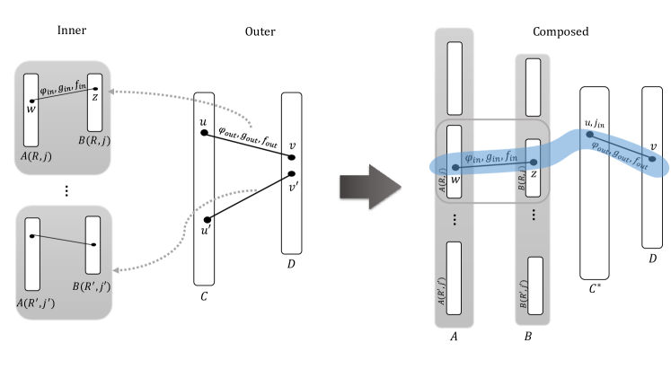
Figure 1: Composition of two 2-prover dPCPs $\mathcal{D}_{\_}{\mathrm{out}}$ and $\mathcal{D}_{\_}{\mathrm{in}}$ to yield composed dPCP $\mathcal{D}_{\_}\mathrm{comp}$. Note that $\mathcal{D}_{\_}{\mathrm{in}},\mathcal{D}_{\_}{\mathrm{out}}$ make two queries each, and $\mathcal{D}_{\_}\mathrm{comp}$ makes four queries: $w,z,(u,j_{\_}{\mathrm{in}}),v$ to $A,B,C^{*},D$ respectively.

The main goal of composition is to reduce the answer size of the outer PCP decoder. By this we are referring to the answer size of the large prover; as it is always possible to reduce the answer size of projection provers at negligible cost. For simplicity, let us assume that each of the inner and the outer PCP decoders use only two provers. The inner PCP decoder $\mathcal{D}_{\_}{\mathrm{in}}$ interacts with provers $A$ and $B$, and the outer PCP decoder $\mathcal{D}_{\_}{\mathrm{out}}$ interacts with provers $C$ and $D$. The composed PCP decoder $\mathcal{D}_{\_}\mathrm{comp}$ works as follows: On input $\left(\Phi,F\right)$, $\mathcal{D}_{\_}\mathrm{comp}$ simulates $\mathcal{D}_{\_}{\mathrm{out}}$ to obtain the tuple $\left(q_{\_}{\mathrm{out}},\varphi_{\_}{\mathrm{out}},g_{\_}{\mathrm{out}},f_{\_}{\mathrm{out}}\right)$. Letting $q_{\_}{\mathrm{out}}=(u,v)$ we picture this as an edge in the bipartite graph of the outer dPCP, and we label this edge with $\left(\varphi_{\_}{\mathrm{out}},g_{\_}{\mathrm{out}},f_{\_}{\mathrm{out}}\right)$. In its normal running $\mathcal{D}_{\_}{\mathrm{out}}$ generates queries $q_{\_}{\mathrm{out}}=(u,v)$ and queries $C$ on $u$ and $D$ on $v$. It then checks that $\varphi_{\_}{\mathrm{out}}(C(u))=0$ and $g_{\_}{\mathrm{out}}(C(u))=D(v)$ and if so it outputs $f_{\_}{\mathrm{out}}(C(u))$.

However, the answer $C(u)$ is too large for $\mathcal{D}_{\_}\mathrm{comp}$, and we would like to use the inner PCP decoder $\mathcal{D}_{\_}{\mathrm{in}}$ to replace querying $C$ directly, reducing the answer size at the cost of a few extra queries. For this purpose, the composed PCP decoder $\mathcal{D}_{\_}\mathrm{comp}$ now simulates the inner PCP decoder $\mathcal{D}_{\_}{\mathrm{in}}$ on input $\left(\varphi_{\_}{\mathrm{out}},\left(g_{\_}{\mathrm{out}},f_{\_}{\mathrm{out}}\right)\right)$ to generate the tuple $\left(q_{\_}{\mathrm{in}},\varphi_{\_}{\mathrm{in}},g_{\_}{\mathrm{in}},f_{\_}{\mathrm{in}}\right)$. The composed PCP decoder $\mathcal{D}_{\_}\mathrm{comp}$ then queries the inner provers $A,B$ on queries $q_{\_}{\mathrm{in}}=(w,z)$ to obtain the answers $\alpha=A(w)$ and $\beta=B(z)$. It then performs the projection tests $g_{\_}{\mathrm{in}}$ of the inner PCP decoder $\mathcal{D}_{\_}{\mathrm{in}}$ and produces its output $f_{\_}{\mathrm{in}}\left(\alpha\right)$. These answers are then used to both perform the projection test of the outer PCP decoder as well as produce the required output of the outer PCP decoder.

As usual in composition, we need to enforce consistency between the different invocations of $\mathcal{D}_{\_}{\mathrm{in}}$. The input for $\mathcal{D}_{\_}{\mathrm{in}}$, namely $\left(q_{\_}{\mathrm{in}},\varphi_{\_}{\mathrm{in}},g_{\_}{\mathrm{in}},f_{\_}{\mathrm{in}}\right)$, is generated using $\mathcal{D}_{\_}{\mathrm{out}}$’s randomness, namely $R$ and $j$. The provers $A$ and $B$ must be told this input because they need to know what they are supposed to prove. Thus $A$ and $B$ are actually aggregates of prover-pairs $A(R,j),B(R,j)$ ranging over all possible $R,j$. There is a possibility that they could “cheat” by outputting a different answer for the same outer question, depending on $R$ and $j$. In particular, think of two outer query pairs $(u,v_{\_}1)$ and $(u,v_{\_}2)$ generated by two different random strings $R_{\_}1,j_{\_}1$ and $R_{\_}2,j_{\_}2$. We need to ensure that both invocations of $\mathcal{D}_{\_}{\mathrm{in}}$ are consistent with the same answer $C(u)$.

We address this issue using the decoding feature of the inner PCP decoder $\mathcal{D}_{\_}{\mathrm{in}}$. We replace the outer prover $C$ by a prover $C^{*}$, which we call the consistency prover. This prover is supposed to hold an encoding, via $E_{\_}{\mathrm{in}}$, of the outer prover $C$. The composed PCP decoder $\mathcal{D}_{\_}\mathrm{comp}$ expects the inner PCP decoder $\mathcal{D}_{\_}{\mathrm{in}}$ to decode a random symbol in this encoding (i.e., in $E_{\_}{\mathrm{in}}\left(C(u)\right)$). This decoded value is then checked against the consistency prover $C^{*}$, which unlike the inner provers is not informed of the outer randomness $R$. In all, the queries of $\mathcal{D}_{\_}\mathrm{comp}$ are $w,z,(u,j_{\_}{\mathrm{in}}),v$ to $A,B,C^{*},D$ respectively.

This additional consistency query helps us get around the above mentioned issue at a small additional cost of $\eta_{\_}{\mathrm{in}}$ in the soundness error, where $\eta_{\_}{\mathrm{in}}$ is the agreement parameter of the encoding $E_{\_}{\mathrm{in}}$ (see Remark 2.4).

It can be shown that this consistency query ensures that the distributional soundness error of the composed decoder is at most the sum of the distributional soundness errors of the outer and inner PCP decoders and the agreement parameter of the encoding $E_{\_}{\mathrm{in}}$. Previous soundness analyses using list-decoding soundness typically involved a $L_{\_}{\mathrm{in}}$-fold multiplicative blowup in the soundness error $\delta_{\_}{\mathrm{out}}$ of the outer PCP decoder (i.e., $\delta_{\_}\mathrm{comp}\geq L_{\_}{\mathrm{in}}\cdot\delta_{\_}{\mathrm{out}}$) where $L_{\_}{\mathrm{in}}$ is the list-size of the inner PCP decoder. Distributional soundness has the advantage of getting rid of this $L_{\_}{\mathrm{in}}$-fold blowup at the cost an additional $\eta_{\_}{\mathrm{in}}$ additive error.

The above description easily generalizes to $k>2$ by replacing $B$ by $B_{\_}1,\ldots,B_{\_}{k_{\_}{\mathrm{in}}-1}$ and $D$ by $D_{\_}1,\ldots,D_{\_}{k_{\_}{\mathrm{out}}-1}$.

As in the case of the definition of decodable PCPs, we find it sufficient to describe composition of algebraic dPCPs and not general dPCPs.

Theorem 4.1 (Composition Theorem).

Let $\mathbb{F}$ be a finite field. Suppose that $N_{\_}{\mathrm{out}},N_{\_}{\mathrm{in}},r_{\_}{\mathrm{out}},r_{\_}{\mathrm{in}},s_{\_}{\mathrm{out}},$ $s_{\_}{\mathrm{in}},n_{\_}{\mathrm{out}},n_{\_}{\mathrm{in}},$ $t_{\_}{\mathrm{out}},t_{\_}{\mathrm{in}},k_{\_}{\mathrm{out}},k_{\_}{\mathrm{in}},l_{\_}{\mathrm{out}},l_{\_}{\mathrm{in}}\in\mathbb{Z}^{+}$, and $\delta_{\_}{\mathrm{out}},\delta_{\_}{\mathrm{in}},\eta_{\_}{\mathrm{in}}\in[0,1]$ are such that

• Alg-CktSAT has a $k_{\_}{\mathrm{out}}$-prover $l_{\_}{\mathrm{out}}$-answer decodable PCP $\mathcal{D}_{\_}{\mathrm{out}}$ with respect to encoding $E_{\_}{\mathrm{out}}:\mathbb{F}^{n_{\_}{\mathrm{out}}}\to\mathbb{F}^{t_{\_}{\mathrm{out}}}$ with randomness complexity $r_{\_}{\mathrm{out}}$, answer size $s_{\_}{\mathrm{out}}$, and distributional soundness error $\delta_{\_}{\mathrm{out}}$ on inputs $\Phi$ of size $N_{\_}{\mathrm{out}}$,

• $\mbox{{{Alg-CktSAT}}}_{\_}\mathbb{F}$ has a $k_{\_}{\mathrm{in}}$-prover $l_{\_}{\mathrm{in}}$-answer decodable PCP $\mathcal{D}_{\_}{\mathrm{in}}$ with respect to encoding $E_{\_}{\mathrm{in}}:\mathbb{F}^{n_{\_}{\mathrm{in}}}\to\mathbb{F}^{t_{\_}{\mathrm{in}}}$ with randomness complexity $r_{\_}{\mathrm{in}}$, answer size $s_{\_}{\mathrm{in}}$, and distributional soundness soundness error $\delta_{\_}{\mathrm{in}}$ on inputs $\varphi$ of size $N_{\_}{\mathrm{in}}$

• $s_{\_}{\mathrm{out}}\leq n_{\_}{\mathrm{in}}\leq N_{\_}{\mathrm{in}}$,

• $l_{\_}{\mathrm{in}}=k_{\_}{\mathrm{out}}+l_{\_}{\mathrm{out}}$,

• the inner encoding $E_{\_}{\mathrm{in}}$ has agreement parameter $\eta_{\_}{\mathrm{in}}$

Then, Alg-CktSAT has a $k_{\_}{\mathrm{out}}+k_{\_}{\mathrm{in}}$-prover $l_{\_}{\mathrm{out}}$-answer dPCP, denoted $\mathcal{D}_{\_}\mathrm{comp}=\mathcal{D}_{\_}{\mathrm{out}}\circledast\mathcal{D}_{\_}{\mathrm{in}}$, with respect to encoding $E_{\_}{\mathrm{out}}$ on inputs $\Phi$ of size $N$ with

• randomness complexity $r_{\_}{\mathrm{out}}+r_{\_}{\mathrm{in}}+\log_{\_}2(t_{\_}{\mathrm{in}})$,

• answer size $s_{\_}{\mathrm{in}}$, and

• distributional soundness error $\delta_{\_}{\mathrm{out}}+\delta_{\_}{\mathrm{in}}+\eta_{\_}{\mathrm{in}}.$

Furthermore, there exists a universal algorithm with black-box access to $\mathcal{D}_{\_}{\mathrm{out}}$ and $\mathcal{D}_{\_}{\mathrm{in}}$ that can perform the actions of $\mathcal{D}_{\_}\mathrm{comp}$ (i.e. evaluating $\mathcal{D}_{\_}\mathrm{comp}\left(\Phi,F;R,j\right)$). On inputs of size $N$, this algorithm runs in time $N^{c}$ for a universal constant $c$, with one call to $\mathcal{D}_{\_}{\mathrm{out}}$ on an input of size $N$ and one call to $\mathcal{D}_{\_}{\mathrm{in}}$ on an input of size $s_{\_}{\mathrm{out}}$.

Proof.

We will follow the following notation to describe the composed decoder.

Provers of $\mathcal{D}_{\_}\mathrm{comp}$

Suppose the inner PCP decoder $\mathcal{D}_{\_}{\mathrm{in}}$ interacts with provers $A,B_{\_}1,\dots,B_{\_}{k_{\_}{\mathrm{in}}-1}$ (here $A$ is the large prover and $B_{\_}i$’s are the projection provers), and the outer PCP decoder interacts with provers $C,D_{\_}1,\dots,D_{\_}{k_{\_}{\mathrm{out}}-1}$ (here $C$ is the large prover and $D_{\_}i$’s are the projection provers).

As mentioned in the informal description, the composed PCP decoder $\mathcal{D}_{\_}\mathrm{comp}$ simulates $\mathcal{D}_{\_}{\mathrm{out}}$ except that instead of querying $C$, uses the inner PCP decoder $\mathcal{D}_{\_}{\mathrm{in}}$ and an additional consistency prover $C^{*}$. Thus, the provers for the composed PCP decoder $\mathcal{D}_{\_}\mathrm{comp}$ will be the following: $A,B_{\_}1,\dots,B_{\_}{k_{\_}{\mathrm{in}}-1},C^{*},D_{\_}1,\dots,D_{\_}{k_{\_}{\mathrm{out}}-1}$; the main prover being $A$ and the projection provers being the rest. As mentioned in the outline, for each choice of the outer randomness $R_{\_}{\mathrm{out}}$ and index $j_{\_}{\mathrm{out}}$ the inner PCP decoder $\mathcal{D}_{\_}{\mathrm{in}}$ is simulated on a different input. Hence the corresponding inner provers for the composed dPCP $\mathcal{D}_{\_}\mathrm{comp}$ (i.e., $A,B_{\_}1,\dots,B_{\_}{k_{\_}{\mathrm{in}}-1}$) are explicitly given the specification of the outer randomness $R_{\_}{\mathrm{out}}$ and index $j_{\_}{\mathrm{out}}$ as part of their queries. (Alternatively, one can think of $A$ and $B_{\_}i$ as an aggregate of separate provers $A(R_{\_}{\mathrm{out}},j_{\_}{\mathrm{out}})$ and $B_{\_}i(R_{\_}{\mathrm{out}},j_{\_}{\mathrm{out}})$ per $R_{\_}{\mathrm{out}},j_{\_}{\mathrm{out}}$).

Randomness of $\mathcal{D}_{\_}\mathrm{comp}$

The randomness of $\mathcal{D}_{\_}\mathrm{comp}$ comes in three parts: the randomness $R_{\_}{\mathrm{out}}$ of $\mathcal{D}_{\_}{\mathrm{out}}$, the randomness $R_{\_}{\mathrm{in}}$ of $\mathcal{D}_{\_}{\mathrm{in}}$ and a random index $j_{\_}{\mathrm{in}}$ to perform the consistency test. Thus, $R_{\_}\mathrm{comp}=\left(R_{\_}{\mathrm{out}},R_{\_}{\mathrm{in}},j_{\_}{\mathrm{in}}\right)$.

Decoded Index of $\mathcal{D}_{\_}\mathrm{comp}$

The index $j_{\_}\mathrm{comp}$ being decoded by $\mathcal{D}_{\_}\mathrm{comp}$ is passed as the index $j_{\_}{\mathrm{out}}$ being decoded by $\mathcal{D}_{\_}{\mathrm{out}}$.

Indexing the answers of $\mathcal{D}_{\_}\mathrm{comp}$

Note that the number of answers $l_{\_}{\mathrm{in}}$ of the inner PCP decoder $\mathcal{D}_{\_}{\mathrm{in}}$ is the sum of the number of answers $l_{\_}{\mathrm{out}}$ of the outer $\mathcal{D}_{\_}{\mathrm{out}}$ and the number of provers $k_{\_}{\mathrm{out}}$ of outer $\mathcal{D}_{\_}{\mathrm{out}}$. Thus, $f_{\_}{\mathrm{in}}$ is a list of $l_{\_}{\mathrm{out}}+k_{\_}{\mathrm{out}}$ functions. We will find it convenient to index the functions in $f_{\_}{\mathrm{in}}$ with $\left\{0\right\}\cup\left(\left\{{\mathrm{out}}\right\}\times\{0,1,\dots,l_{\_}{\mathrm{out}}-1\}\right)\cup\left(\left\{{\mathrm{proj}}\right\}\times\{1,\dots,k_{\_}{\mathrm{out}}-1\}\right)$, such that $f_{\_}{{\mathrm{in}},({\mathrm{proj}},i)}$, $i=1,\ldots,k_{\_}{\mathrm{out}}-1$, are the answers to be compared with the outer projection provers, $f_{\_}{{\mathrm{in}},0}$ is intended for the consistency test, and $f_{\_}{{\mathrm{in}},({\mathrm{out}},i)}$, $i=0,\ldots,\ell_{\_}{\mathrm{out}}-1$, give the answers for the outer decoder.

With these conventions in place, here is the description of the composed PCP decoder, $\mathcal{D}_{\_}\mathrm{comp}$:

$\mathcal{D}_{\_}\mathrm{comp}(\Phi,F;R_{\_}{\mathrm{out}},R_{\_}{\mathrm{in}},j_{\_}{\mathrm{in}})$: • Input: $\left(\Phi,F\right)$ • Random input string: $\left(R_{\_}{\mathrm{out}},R_{\_}{\mathrm{in}},j_{\_}{\mathrm{in}}\right)$ • Index to be decoded: $j_{\_}{\mathrm{out}}$ • Provers: $\Pi=\left(A,B_{\_}1,\dots,B_{\_}{k_{\_}{\mathrm{in}}-1},C^{*},D_{\_}1,\dots,D_{\_}{k_{\_}{\mathrm{out}}-1}\right)$ 1. Initial Computation: (a) [Simulating $\mathcal{D}_{\_}{\mathrm{out}}$] Run $\mathcal{D}_{\_}{\mathrm{out}}\left(\Phi,F;R_{\_}{\mathrm{out}},j_{\_}{\mathrm{out}}\right)$ to obtain $\left(q_{\_}{\mathrm{out}},\varphi_{\_}{\mathrm{out}},g_{\_}{\mathrm{out}},f_{\_}{\mathrm{out}}\right)$. (b) [Simulating $\mathcal{D}_{\_}{\mathrm{in}}$] Run $\mathcal{D}_{\_}{\mathrm{in}}\left(\varphi_{\_}{\mathrm{out}},\left(g_{\_}{\mathrm{out}},f_{\_}{\mathrm{out}}\right);R_{\_}{\mathrm{in}},j_{\_}{\mathrm{in}}\right)$ to obtain $\left(q_{\_}{\mathrm{in}},\varphi_{\_}{\mathrm{in}},g_{\_}{\mathrm{in}},f_{\_}{\mathrm{in}}\right)$. 2. Queries: Let $q_{\_}{\mathrm{out}}=(u,v_{\_}1,\ldots,v_{\_}{k_{\_}{\mathrm{out}}-1})$ and let $q_{\_}{\mathrm{in}}=(w,z_{\_}1,\ldots,z_{\_}{k_{\_}{\mathrm{in}}-1})$. (a) Send query $\left(R_{\_}{\mathrm{out}},j_{\_}{\mathrm{out}},w\right)$ to prover $A$ to obtain answer $\alpha=A(R_{\_}{\mathrm{out}},j_{\_}{\mathrm{out}},w)$. (b) For $i=1,\ldots,k_{\_}{{\mathrm{in}}-1}$, send query $\left(R_{\_}{\mathrm{out}},j_{\_}{\mathrm{out}},z_{\_}i\right)$ to prover $B_{\_}i$ to obtain answer $\beta_{\_}{i}=B_{\_}i(R_{\_}{\mathrm{out}},j_{\_}{\mathrm{out}},z_{\_}i)$. (c) Send query $\left(u,j_{\_}{\mathrm{in}}\right)$ to prover $C^{*}$ to obtain answer $\gamma=C^{*}(u,j_{\_}{\mathrm{in}})$. (d) For $i=1\dots,k_{\_}{{\mathrm{out}}}-1$, send query $v_{\_}i$ to prover $D_{\_}i$ to obtain answer $\zeta_{\_}{i}=D_{\_}i(v_{\_}i)$. 3. Checks: (a) [Inner local predicate] Check that $\varphi_{\_}{\mathrm{in}}\left(\alpha\right)=1$. (b) [Inner projection tests] For $i=1,\dots,k_{\_}{{\mathrm{in}}-1}$, check that $g_{\_}{{\mathrm{in}},i}\left(\alpha\right)=\beta_{\_}{i}$. (c) [Consistency test] Check that $f_{\_}{{\mathrm{in}},0}\left(\alpha\right)=\gamma$. (d) [Outer projection tests] For $i=1,\dots,k_{\_}{{\mathrm{out}}-1}$, check that $f_{\_}{{\mathrm{in}},\left({\mathrm{proj}},i\right)}\left(\alpha\right)=\zeta_{\_}{i}.$ 4. Output: If all the checks in the above step pass, then return $f_{\_}{{\mathrm{in}},\left({\mathrm{out}},\cdot\right)}\left(\alpha\right)$ else return $\bot$.

The claims about $\mathcal{D}_{\_}\mathrm{comp}$’s parameters (randomness complexity, answer size, number of provers, number of answers) except completeness and soundness error can be verified by inspection. Thus, we only need to check completeness and soundness.

Completeness

Let $x\in SAT\left(\Phi\right)$. By the completeness of outer $\mathcal{D}_{\_}{\mathrm{out}}$, there exist provers $\Pi^{\mathrm{out}}=\left(C,D_{\_}1,\dots,D_{\_}{k_{\_}{\mathrm{out}}-1}\right)$, such that for all $\left(R_{\_}{\mathrm{out}},j_{\_}{\mathrm{out}}\right)$ we have

$$\mathcal{D}^{\Pi^{\mathrm{out}}}_{\_}{\mathrm{out}}\left(\Phi,F;R_{\_}{\mathrm{out}},j_{\_}{\mathrm{out}}\right)=\left(E_{\_}{\mathrm{out}}\left(x\right)_{\_}{j_{\_}{{\mathrm{out}}}},F_{\_}1\left(x\right),\dots,F_{\_}{l_{\_}{\mathrm{out}}}\left(x\right)\right).$$

Fix any particular outer random string $R_{\_}{\mathrm{out}}$ and index $j_{\_}{\mathrm{out}}$. Let $\mathcal{D}_{\_}{\mathrm{out}}\left(\Phi,F;R_{\_}{\mathrm{out}},j_{\_}{\mathrm{out}}\right)=\left(q_{\_}{\mathrm{out}},\varphi_{\_}{\mathrm{out}},g_{\_}{\mathrm{out}},f_{\_}{\mathrm{out}}\right)$. Since the outer decoder $\mathcal{D}_{\_}{\mathrm{out}}$ does not reject, we must have that $y_{\_}{\left(R_{\_}{\mathrm{out}},j_{\_}{\mathrm{out}}\right)}:=C(u)$ satisfies $\varphi_{\_}{\mathrm{out}}$. In other words, $y_{\_}{\left(R_{\_}{\mathrm{out}},j_{\_}{\mathrm{out}}\right)}\in\mbox{{{SAT}}}\left(\varphi_{\_}{\mathrm{out}}\right)$. Now, by the completeness of the inner $\mathcal{D}_{\_}{\mathrm{in}}$, we have that for these $\left(R_{\_}{\mathrm{out}},j_{\_}{\mathrm{out}}\right)$ there exist provers $\Pi^{{\mathrm{in}}}_{\_}{\left(R_{\_}{\mathrm{out}},j_{\_}{\mathrm{out}}\right)}=\left(A_{\_}{\left(R_{\_}{\mathrm{out}},j_{\_}{\mathrm{out}}\right)},B_{\_}{\left(R_{\_}{\mathrm{out}},j_{\_}{\mathrm{out}}\right),1},\dots,B_{\_}{\left(R_{\_}{\mathrm{out}},j_{\_}{\mathrm{out}}\right),k_{\_}{\mathrm{in}}-1}\right)$ such that for all $\left(R_{\_}{\mathrm{in}},j_{\_}{\mathrm{in}}\right)$ we have

$$\mathcal{D}^{\Pi^{{\mathrm{in}}}_{\_}{\left(R_{\_}{\mathrm{out}},j_{\_}{\mathrm{out}}\right)}}_{\_}{\mathrm{in}}\left(\varphi_{\_}{\mathrm{out}},\left(g_{\_}{\mathrm{out}},f_{\_}{\mathrm{out}}\right);R_{\_}{\mathrm{in}},j_{\_}{\mathrm{in}}\right)=\left(E_{\_}{\mathrm{in}}\left(y_{\_}{\left(R_{\_}{\mathrm{out}},j_{\_}{\mathrm{out}}\right)}\right)_{\_}{j_{\_}{\mathrm{in}}},g_{\_}{\mathrm{out}}\left(y_{\_}{\left(R_{\_}{\mathrm{out}},j_{\_}{\mathrm{out}}\right)}\right),f_{\_}{\mathrm{out}}\left(y_{\_}{\left(R_{\_}{\mathrm{out}},j_{\_}{\mathrm{out}}\right)}\right)\right).$$

We are now ready to define the provers

$$\Pi=\left(A,B_{\_}1,\dots,B_{\_}{k_{\_}{\mathrm{in}}-1},C^{*},D_{\_}1,\dots,D_{\_}{k_{\_}{\mathrm{out}}-1}\right)$$

for the composed decoder $\mathcal{D}_{\_}\mathrm{comp}$. As the name suggests, the projection provers $D_{\_}i,i=1,\dots,k_{\_}{{\mathrm{out}}}-1$ are exactly the same as the outer projection provers in $\Pi^{\mathrm{out}}$. The consistency prover $C^{*}$ is defined by encoding $C(u)$ separately for each $u$ as

$$C^{*}\left(u,j_{\_}{\mathrm{in}}\right):=E_{\_}{\mathrm{in}}\left(C(u)\right)_{\_}{j_{\_}{\mathrm{in}}}.$$

The projection provers $B_{\_}i,i=1,\dots,k_{\_}{{\mathrm{in}}}-1$ are defined as $B_{\_}i\left(R_{\_}{\mathrm{out}},j_{\_}{\mathrm{out}},z_{\_}i\right):=B_{\_}{\left(R_{\_}{\mathrm{out}},j_{\_}{\mathrm{out}}\right),i}\left(z_{\_}i\right)$. Finally, the large prover $A$ is defined as $A\left(R_{\_}{\mathrm{out}},j_{\_}{\mathrm{out}},w\right):=A_{\_}{\left(R_{\_}{\mathrm{out}},j_{\_}{\mathrm{out}}\right)}(w)$. It is easy to check that according to this definition of $\Pi$, for each $\left(\left(R_{\_}{\mathrm{out}},R_{\_}{\mathrm{in}},j_{\_}{\mathrm{in}}\right),j_{\_}{\mathrm{out}}\right)$ it holds that

$$\mathcal{D}^{\Pi}_{\_}\mathrm{comp}\left(\Phi,F;\left(R_{\_}{\mathrm{out}},R_{\_}{\mathrm{in}},j_{\_}{\mathrm{in}}\right),j_{\_}{\mathrm{out}}\right)=\left(E_{\_}{\mathrm{out}}\left(x\right)_{\_}{j_{\_}{\mathrm{out}}},F_{\_}1\left(x\right),\dots,F_{\_}{l_{\_}{\mathrm{out}}}\left(x\right)\right).$$

This proves the completeness of $\mathcal{D}_{\_}\mathrm{comp}$.∎

Distributional Soundness of $\mathcal{D}_{\_}\mathrm{comp}$

We prove the following statement about the distributional soundness of $\mathcal{D}_{\_}\mathrm{comp}$.

Lemma 4.2.

Suppose the outer PCP decoder $\mathcal{D}_{\_}{\mathrm{out}}$ has distributional soundness error $\delta_{\_}{\mathrm{out}}$ with respect to encoding $E_{\_}{\mathrm{out}}$, and the inner PCP decoder $\mathcal{D}_{\_}{\mathrm{in}}$ has distributional soundness error $\delta_{\_}{\mathrm{in}}$ with respect to encoding $E_{\_}{\mathrm{in}}$, and suppose $E_{\_}{\mathrm{in}}$ has agreement parameter $\eta_{\_}{\mathrm{in}}$ (see Remark 2.4). Then, the composed PCP decoder $\mathcal{D}_{\_}\mathrm{comp}=\mathcal{D}_{\_}{\mathrm{out}}\circledast\mathcal{D}_{\_}{\mathrm{in}}$ has distributional soundness error $\delta_{\_}\mathrm{comp}\leq\delta_{\_}{\mathrm{out}}+\delta_{\_}{\mathrm{in}}+\eta_{\_}{\mathrm{in}}$ with respect to encoding $E_{\_}{\mathrm{out}}$.

Proof.

Suppose $\mathcal{D}_{\_}\mathrm{comp}$ on input $\left(\Phi,F\right)$ interacts with provers

$$\Pi=\left(A,B_{\_}1,\ldots,B_{\_}{k_{\_}{\mathrm{in}}-1},C^{*},D_{\_}1,\ldots,D_{\_}{k_{\_}{\mathrm{out}}-1}\right).$$

To prove soundness of $\mathcal{D}_{\_}\mathrm{comp}$, we need to construct for each composed random string $R_{\_}\mathrm{comp}:=\left(R_{\_}{\mathrm{out}},R_{\_}{\mathrm{in}},j_{\_}{\mathrm{in}}\right)$, functions ${\widetilde{x}}\left(R_{\_}\mathrm{comp}\right)$ and ${\widetilde{\Pi}}\left(R_{\_}\mathrm{comp}\right)$ such that ${\widetilde{\Pi}}\left(R_{\_}\mathrm{comp}\right)$ is either $\bot$ or a valid proof for the statement ${\widetilde{x}}\left(R_{\_}\mathrm{comp}\right)\in\mbox{{{SAT}}}\left(\Phi\right)$, and for every $j_{\_}{\mathrm{out}}$ we have

$$\Pr_{\_}{R_{\_}\mathrm{comp}}\left[\mathcal{D}_{\_}\mathrm{comp}^{\Pi}\left(\Phi,F;R_{\_}\mathrm{comp},j_{\_}{\mathrm{out}}\right)=\bot\text{ or }\Pi|_{\_}{q_{\_}\mathrm{comp}}={\widetilde{\Pi}}\left(R_{\_}\mathrm{comp}\right)|_{\_}{q_{\_}\mathrm{comp}}\right]\geq 1-(\delta_{\_}{\mathrm{out}}+\delta_{\_}{\mathrm{in}}+\eta_{\_}{\mathrm{in}}),$$

where $q_{\_}\mathrm{comp}$ is the query vector generated by $\mathcal{D}_{\_}\mathrm{comp}$.

The construction of ${\widetilde{x}}\left(R_{\_}\mathrm{comp}\right)$ and ${\widetilde{\Pi}}\left(R_{\_}\mathrm{comp}\right)$ relies on the soundness properties of $\mathcal{D}_{\_}{\mathrm{out}}$ and $\mathcal{D}_{\_}{\mathrm{in}}$. We first locally-decode $C^{*}$ to obtain a distribution over outer provers $C$. We then use the distributional soundness of $\mathcal{D}_{\_}{\mathrm{out}}$ to obtain an idealized outer proof $(\widetilde{C},\widetilde{D}_{\_}i)$. We then use the soundness of $\mathcal{D}_{\_}{\mathrm{in}}$ to obtain idealized inner proofs $(\widetilde{A},\widetilde{B}_{\_}i)$.

Outer main prover $C_{\_}{j_{\_}{\mathrm{in}}}$:

For each $j_{\_}{\mathrm{in}}$, we define an outer main prover $C_{\_}{j_{\_}{\mathrm{in}}}$ using the consistency prover $C^{*}$ as follows. Let $\tau=\eta_{\_}{\mathrm{in}}/2$ be the agreement parameter of $E_{\_}{\mathrm{in}}$, as in Remark 2.4. For each query $u:=q_{\_}{{\mathrm{out}},0}$ to the outer main prover, $C_{\_}{j_{\_}{\mathrm{in}}}\left(u\right)$ is defined to be the $j_{\_}{{\mathrm{in}}}$-th entry of the $\tau$-local decoding of $C^{*}\left(u,\cdot\right)$ as in Definition 2.2 if well-defined and $\bot$ otherwise. color=blue!25!, size=]Irit: removed the explicit def, see latex

Idealized outer pairs ${\widetilde{x}}^{\mathrm{out}}_{\_}{j_{\_}{\mathrm{in}}}\left(R_{\_}{\mathrm{out}}\right)$ and ${\widetilde{\Pi}}^{\mathrm{out}}_{\_}{j_{\_}{\mathrm{in}}}\left(R_{\_}{\mathrm{out}}\right)$:

For each $j_{\_}{\mathrm{in}}$ we have an outer proof

$$\Pi^{\mathrm{out}}_{\_}{j_{\_}{\mathrm{in}}}=\left(C_{\_}{j_{\_}{\mathrm{in}}},D_{\_}1,\ldots,D_{\_}{k_{\_}{\mathrm{out}}-1}\right).$$

Note that only the $C$ provers are different in the various outer provers $\Pi^{\mathrm{out}}_{\_}{j_{\_}{\mathrm{in}}}$ as we range over $j_{\_}{\mathrm{in}}$. From the soundness of $\mathcal{D}_{\_}{\mathrm{out}}$ for every $\Pi^{\mathrm{out}}_{\_}{j_{\_}{\mathrm{in}}}$ there is an idealized pair ${\widetilde{x}}^{\mathrm{out}}_{\_}{j_{\_}{\mathrm{in}}}\left(R_{\_}{\mathrm{out}}\right)$ and ${\widetilde{\Pi}}^{\mathrm{out}}_{\_}{j_{\_}{\mathrm{in}}}\left(R_{\_}{\mathrm{out}}\right)=\left(\widetilde{C},\widetilde{D}_{\_}1,\ldots,\widetilde{D}_{\_}{k_{\_}{\mathrm{out}}-1}\right)$ that “explain” its success. color=blue!25!, size=]Irit: removed repeating of definition, see latex

Idealized inner pairs $\widetilde{y}^{\mathrm{in}}_{\_}{\left(R,j\right)}\left(R_{\_}{\mathrm{in}}\right)$ and ${\widetilde{\Pi}}^{\mathrm{in}}_{\_}{\left(R,j\right)}\left(R_{\_}{\mathrm{in}}\right)$:

For every outer randomness $R$ and index $j$ let

$$\Pi^{\mathrm{in}}_{\_}{\left(R,j\right)}:=\left(A\left(R,j,\cdot\right),B_{\_}1\left(R,j,\cdot\right),\ldots,B_{\_}{k_{\_}{\mathrm{in}}-1}\left(R,j,\cdot\right)\right)$$

be the relevant part of the proof for $\mathcal{D}_{\_}{\mathrm{in}}$.

Let $\left(q,\varphi,g,f\right)=\mathcal{D}_{\_}{\mathrm{out}}\left(\Phi,F;R,j\right)$. When $R_{\_}{\mathrm{out}}=R$ and $j_{\_}{\mathrm{out}}=j$, the composed decoder $\mathcal{D}_{\_}\mathrm{comp}$ simulates running $\mathcal{D}_{\_}{\mathrm{in}}$ with input $\left(\varphi,\left({g},f\right);R_{\_}{\mathrm{in}},j_{\_}{\mathrm{in}}\right)$ and with the proof $\Pi^{\mathrm{in}}_{\_}{\left(R,j\right)}$.

For each $\Pi^{\mathrm{in}}_{\_}{(R,j)}$, the soundness of $\mathcal{D}_{\_}{\mathrm{in}}$ guarantees idealized prover pairs $\widetilde{y}^{\mathrm{in}}_{\_}{\left(R,j\right)}$ and ${\widetilde{\Pi}}^{\mathrm{in}}_{\_}{\left(R,j\right)}$ (functions of $R_{\_}{\mathrm{in}}$) that ”explain” its success. color=blue!25!, size=]Irit: again removed repeating the properties of ${\widetilde{\Pi}}$ from the def

We are ready to define the idealized $(\widetilde{x},{\widetilde{\Pi}})$ pairs for the composed decoder $\mathcal{D}_{\_}\mathrm{comp}$.

Idealized composed pairs ${\widetilde{x}}\left(R_{\_}\mathrm{comp}\right)$ and ${\widetilde{\Pi}}\left(R_{\_}\mathrm{comp}\right)$:

Recall that $R_{\_}\mathrm{comp}$ is short for $\left(R_{\_}{\mathrm{out}},R_{\_}{\mathrm{in}},j_{\_}{\mathrm{in}}\right)$. Define ${\widetilde{x}}\left(R_{\_}\mathrm{comp}\right):={\widetilde{x}}^{\mathrm{out}}_{\_}{j_{\_}{\mathrm{in}}}\left(R_{\_}{\mathrm{out}}\right)$. We then set ${\widetilde{\Pi}}\left(R_{\_}\mathrm{comp}\right)$ as follows: If ${\widetilde{\Pi}}^{\mathrm{out}}_{\_}{j_{\_}{\mathrm{in}}}\left(R_{\_}{\mathrm{out}}\right)$ is successful, in particular $C_{\_}{j_{\_}{\mathrm{in}}}(u)=\widetilde{C}(u)$, set ${\widetilde{\Pi}}\left(R_{\_}\mathrm{comp}\right)$ to be the set of provers
$\left({\widetilde{A}},{\widetilde{B}}_{\_}1,\ldots,{\widetilde{B}}_{\_}{k_{\_}{\mathrm{in}}-1},{\widetilde{C}}^{*},{\widetilde{D}}_{\_}1,\ldots,{\widetilde{D}}_{\_}{k_{\_}{\mathrm{out}}-1}\right)$ defined next.

• The outer projection provers ${\widetilde{D}}_{\_}i$ are defined to be the same as in ${\widetilde{\Pi}}^{\mathrm{out}}_{\_}{j_{\_}{\mathrm{in}}}\left(R_{\_}{\mathrm{out}}\right)$.

• Let ${\widetilde{C}}$ be the main prover in ${\widetilde{\Pi}}^{\mathrm{out}}_{\_}{j_{\_}{\mathrm{in}}}\left(R_{\_}{\mathrm{out}}\right)$. We define ${\widetilde{C}}^{*}$ as follows:

  $${\widetilde{C}}^{*}\left(u,j\right):=E_{\_}{\mathrm{in}}\left({\widetilde{C}}(u)\right)_{\_}j.$$

• For any pair $(R,j)$ where $R\in\left\{0,1\right\}^{r_{\_}{\mathrm{out}}}$ and $j\in[t_{\_}{\mathrm{out}}]$, we define ${\widetilde{A}}\left(R,j,\cdot\right)$ and ${\widetilde{B}}_{\_}i\left(R,j,\cdot\right)$ (for $i=1,\ldots,k_{\_}{\mathrm{in}}-1$) as follows. Denote $\left(q,\varphi,g,f\right)=\mathcal{D}_{\_}{\mathrm{out}}\left(\Phi,F;R,j\right)$ and suppose $q=(u,v_{\_}1,\ldots,v_{\_}{k_{\_}{\mathrm{out}}-1})$. If $\widetilde{y}^{\mathrm{in}}_{\_}{(R,j)}(R_{\_}{\mathrm{in}})={\widetilde{C}}(u)$ and also ${\widetilde{\Pi}}^{\mathrm{in}}_{\_}{\left(R,j\right)}\left(R_{\_}{\mathrm{in}}\right)$ is successful, we set ${\widetilde{A}}\left(R,j,\cdot\right)$ and the provers ${\widetilde{B}}_{\_}i\left(R,j,\cdot\right)$ to be the main prover and projection provers in ${\widetilde{\Pi}}^{\mathrm{in}}_{\_}{\left(R,j\right)}\left(R_{\_}{\mathrm{in}}\right)$ respectively.

  Otherwise, color=blue!25!, size=]Irit: need to add a remark explaining this subtlety if $\widetilde{y}^{\mathrm{in}}_{\_}{(R,j)}(R_{\_}{\mathrm{in}})\neq{\widetilde{C}}(u)$ or ${\widetilde{\Pi}}^{\mathrm{in}}_{\_}{\left(R,j\right)}\left(R_{\_}{\mathrm{in}}\right)$ is not successful, we define ${\widetilde{A}}\left(R,j,\cdot\right)$ and ${\widetilde{B}}_{\_}i\left(R,j,\cdot\right)$ by letting them be some valid proofs for the statement ${\widetilde{C}}(u)\in SAT\left(\varphi\right)$ (Note that ${\widetilde{C}}(u)$ satisfies $\varphi$ since ${\widetilde{\Pi}}^{\mathrm{out}}_{\_}{j_{\_}{\mathrm{in}}}\left(R_{\_}{\mathrm{out}}\right)$ is successful).

If either ${\widetilde{\Pi}}^{\mathrm{out}}_{\_}{j_{\_}{\mathrm{in}}}\left(R_{\_}{\mathrm{out}}\right)$ is not successful or any of the intermediate objects in the above definition are $\bot$, then we set ${\widetilde{\Pi}}\left(R_{\_}\mathrm{comp}\right)$ to $\bot$.

It remains to show that the pair ${\widetilde{x}}\left(R_{\_}\mathrm{comp}\right)$ and ${\widetilde{\Pi}}\left(R_{\_}\mathrm{comp}\right)$ has the desired properties. color=red!20!green!15, size=]ph: Needs more explanation It follows by inspection of the definition of ${\widetilde{\Pi}}\left(R_{\_}\mathrm{comp}\right)$ that whenever it is not $\bot$, it is a valid proof of the statement ${\widetilde{x}}\left(R_{\_}\mathrm{comp}\right)\in SAT\left(\Phi\right)$ and agrees with the local view color=red!20!, size=]Guy: elaborate! of $\Pi$ on input $\left(\Phi,F;R_{\_}\mathrm{comp},j_{\_}{\mathrm{out}}\right)$.

So it remains to show that for every $j_{\_}{\mathrm{out}}$,

$$\Pr_{\_}{R_{\_}\mathrm{comp}}\Bigl{[}{\widetilde{\Pi}}\left(R_{\_}\mathrm{comp}\right)=\bot{\hbox{ and }}\mathcal{D}_{\_}\mathrm{comp}^{\Pi}\left(\Phi,F;R_{\_}\mathrm{comp},j_{\_}{\mathrm{out}}\right)\neq\bot\Bigr{]}\leq\delta_{\_}{\mathrm{out}}+\delta_{\_}{\mathrm{in}}+\eta_{\_}{\mathrm{in}}.$$

We partition the above event intro three parts according to the highest indexed condition among the following three conditions that does not hold — one of them must not hold for ${\widetilde{\Pi}}\left(R_{\_}\mathrm{comp}\right)$ to be equal to $\bot$.

1. ${\widetilde{\Pi}}^{\mathrm{out}}_{\_}{j_{\_}{\mathrm{in}}}\left(R_{\_}{\mathrm{out}}\right)$ is successful, in particular $C_{\_}{j_{\_}{\mathrm{in}}}(u)=\widetilde{C}(u)$.

2. $\widetilde{y}^{\mathrm{in}}_{\_}{\left(R_{\_}{\mathrm{out}},j_{\_}{\mathrm{out}}\right)}\left(R_{\_}{\mathrm{in}}\right)=\widetilde{C}_{\_}{j_{\_}{\mathrm{in}}}(u)$.

3. ${\widetilde{\Pi}}^{\mathrm{in}}_{\_}{\left(R_{\_}{\mathrm{out}},j_{\_}{\mathrm{out}}\right)}\left(R_{\_}{\mathrm{in}}\right)$ is successful.

We separately bound the probability of each event in this partition.

• We bound the probability that Condition 3 does not hold, namely that ${\widetilde{\Pi}}^{\mathrm{in}}_{\_}{\left(R_{\_}{\mathrm{out}},j_{\_}{\mathrm{out}}\right)}\left(R_{\_}{\mathrm{in}}\right)$ is not successful, and yet $\mathcal{D}_{\_}\mathrm{comp}$ does not reject. If $\mathcal{D}_{\_}\mathrm{comp}$ doesn’t reject then in particular checks Check 3a and Check 3b pass, which means that $\mathcal{D}_{\_}{\mathrm{in}}^{\Pi^{\mathrm{in}}_{\_}{(R_{\_}{\mathrm{out}},j_{\_}{\mathrm{out}})}}\left(\varphi_{\_}{\mathrm{out}},\left(g_{\_}{\mathrm{out}},f_{\_}{\mathrm{out}}\right);R_{\_}{\mathrm{in}},j_{\_}{\mathrm{in}}\right)\neq\bot$. But the soundness of $\mathcal{D}_{\_}{\mathrm{in}}$ implies that the probability over the choice of $R_{\_}{\mathrm{in}}$ that this occurs and yet ${\widetilde{\Pi}}^{\mathrm{in}}_{\_}{\left(R_{\_}{\mathrm{out}},j_{\_}{\mathrm{out}}\right)}\left(R_{\_}{\mathrm{in}}\right)$ is not successful is bounded by $\delta_{\_}{\mathrm{in}}$.

• Now we bound the probability that Condition 3 holds, Condition 2 does not hold, and yet $\mathcal{D}_{\_}\mathrm{comp}$ does not reject. When Condition 3 holds, the output of the $\mathcal{D}_{\_}{\mathrm{in}}$ simulation for the encoding is $E_{\_}{\mathrm{in}}\left(y^{\mathrm{in}}_{\_}{\left(R_{\_}{\mathrm{out}},j_{\_}{\mathrm{out}}\right)}\left(R_{\_}{\mathrm{in}}\right)\right)_{\_}{j_{\_}{\mathrm{in}}}$. It is thus enough to bound the probability that $\widetilde{y}^{\mathrm{in}}_{\_}{\left(R_{\_}{\mathrm{out}},j_{\_}{\mathrm{out}}\right)}\left(R_{\_}{\mathrm{in}}\right)\neq\widetilde{C}(u)$ and yet $E_{\_}{\mathrm{in}}\left(\widetilde{y}^{\mathrm{in}}_{\_}{\left(R_{\_}{\mathrm{out}},j_{\_}{\mathrm{out}}\right)}\left(R_{\_}{\mathrm{in}}\right)\right)_{\_}{j_{\_}{\mathrm{in}}}=C^{*}\left(u,j_{\_}{\mathrm{in}}\right)$, i.e. Check 3c passes. Since by definition $C_{\_}{j_{\_}{\mathrm{in}}}(u)$ is the $\tau$-local decoding of $C^{*}\left(u,\cdot\right)$ at position $j_{\_}{\mathrm{in}}$, Claim 2.3 and Remark 2.4 imply that the probability of this event over the choice of $j_{\_}{\mathrm{in}}$ is bounded by the agreement parameter $\eta_{\_}{\mathrm{in}}$.

• It remains to bound the probability that Conditions 3 and 2 hold but Condition 1 does not, and yet $\mathcal{D}_{\_}\mathrm{comp}$ does not reject. When Condition 2 and 3 hold it means that $\widetilde{C}\left(u\right)=\widetilde{y}^{\mathrm{in}}_{\_}{\left(R_{\_}{\mathrm{out}},j_{\_}{\mathrm{out}}\right)}\left(R_{\_}{\mathrm{in}}\right)\in SAT\left(\varphi_{\_}{\mathrm{out}}\right)$ and the output of the simulated $\mathcal{D}_{\_}{\mathrm{in}}$ computed by $\mathcal{D}_{\_}\mathrm{comp}$ is

  $$f_{\_}{\mathrm{in}}\left(A\left(R_{\_}{\mathrm{out}},j_{\_}{\mathrm{out}},w\right)\right)=\left(\left(E_{\_}{\mathrm{in}}\left(\widetilde{C}\left(u\right)\right)_{\_}{j_{\_}{\mathrm{in}}},g_{\_}{\mathrm{out}}\left(\widetilde{C}\left(u\right)\right),f_{\_}{\mathrm{out}}\left(\widetilde{C}\left(u\right)\right)\right)\right).$$

  If $\mathcal{D}_{\_}\mathrm{comp}$ does not reject it means that the values of $g_{\_}{\mathrm{out}}\left(\widetilde{C}(u)\right)$ match the ones obtained from the outer projection provers, to which it is compared in Check 3d. But these are also the values used by $\mathcal{D}_{\_}{\mathrm{out}}$ when it is run on input $\left(\Phi,F;R_{\_}{\mathrm{out}},j_{\_}{\mathrm{out}}\right)$ with the proof ${\widetilde{\Pi}}^{\mathrm{out}}_{\_}{j_{\_}{\mathrm{in}}}$, which means that $\mathcal{D}_{\_}{\mathrm{out}}^{{\widetilde{\Pi}}^{\mathrm{out}}_{\_}{j_{\_}{\mathrm{in}}}}\left(\Phi,F;R_{\_}{\mathrm{out}},j_{\_}{\mathrm{out}}\right)\neq\bot$. But the probability over the choice of $R_{\_}{\mathrm{out}}$ that this happens while Condition 1 fails is bounded by $\delta_{\_}{\mathrm{out}}$, the distributional soundness error of $\mathcal{D}_{\_}{\mathrm{out}}$.

This proves the distributional soundness of $\mathcal{D}_{\_}\mathrm{comp}$.

∎

This completes the proof of the Composition Theorem 4.1. ∎

5 Proof of Main Theorem

Theorem 5.1 (Main Construct).

Every language $L$ in NP has a $O(\lg\lg N/\lg\lg\lg N)$-prover projective PCP with the following parameters. On input a Boolean predicate/circuit $\Phi$ of size $N$, the PCP has

• randomness complexity $O(\lg N)$,

• query complexity $O(\lg\lg N/\lg\lg\lg N)$,

• answer size $O(\lg N/\text{poly}\lg\lg N)$,

• perfect completeness, and

• soundness error $N^{1/(\lg\lg N)^{\Omega(1)}}$.

The PCP with inverse polynomial soundness error stated in Main Theorem 1.7 is obtained by sequentially repeating the above PCP $\text{poly}(\lg\lg N)$ times in a randomness efficient manner.

5.1 Building Blocks

The two building blocks, we need for our construction, are two decodable PCP based on the Reed-Muller code and the Hadamard code respectively. The constructions of both these objects is standard given the requirements of the dPCP. These PCPs are based on two encodings the low-degree encoding LDE and the quadratic Hadamard encoding ${\rm QH}$ respectively. The definition of these codes is given in the next section (§ 6). For the purpose of this section, it suffices that these are error correcting codes with very good distance.

Theorem 5.2 (Reed-Muller based dPCP).

For any finite field $\mathbb{F}$, and parameter $h$ such that $1<h<|\mathbb{F}|^{0.1}$ and any $\ell>0$, there is a 2-prover $\ell+1$-answer decodable PCP $\mathcal{D}$ with respect to the encoding $\mbox{{{LDE}}}_{\_}{\mathbb{F},h}$ for the language $\mbox{{{Alg-CktSAT}}}_{\_}\mathbb{F}$ with the following parameters: On inputs (i) a predicate $\Phi:\mathbb{F}^{n}\to\{0,1\}$ and (ii) functions $F_{\_}1,\ldots,F_{\_}{\ell}:\mathbb{F}^{n}\to\mathbb{F}$ given by arithmetic circuits over $\mathbb{F}$ whose total size is $N$, the dPCP $\mathcal{D}$ has (let $m=\log N/\log h$),

• randomness complexity $O(\log{N}+m\log|\mathbb{F}|)=O(m\log\left|\mathbb{F}\right|)$color=red!20!green!15, size=]ph: ???,

• answer size $s,s^{\prime}=O(m(m+\ell))$,

• and distributional soundness error $1/|\mathbb{F}|^{0.1}$.

Theorem 5.3 (Hadamard based dPCP).

For any finite field $\mathbb{F}$, and any $\ell>0$, there is a 2-prover $\ell+1$-answer decodable PCP $\mathcal{D}_{\_}{{\rm QH},\mathbb{F}}$ with respect to the encoding ${\rm QH}_{\_}\mathbb{F}$ for the language $\mbox{{{Alg-CktSAT}}}_{\_}\mathbb{F}$ with the following parameters: On inputs (i) a predicate $\Phi:\mathbb{F}^{n}\to\{0,1\}$ and (ii) functions $F_{\_}1,\ldots,F_{\_}{\ell}:\mathbb{F}^{n}\to\mathbb{F}$ given by arithmetic circuits over $\mathbb{F}$ whose total size is $N$, the dPCP $\mathcal{D}_{\_}{{\rm QH},\mathbb{F}}$ has

• randomness complexity $O(N^{2}\log|\mathbb{F}|)$,

• answer size $s,s^{\prime}=O(\ell)$,

• perfect completeness, and

• distributional soundness error $\leq 1/|\mathbb{F}|^{0.1}$.

These theorems are proved in Section 6.

5.2 Putting it together (Proof of Theorem 5.1)

By NP-completeness of CktSAT it suffices to prove Theorem 5.1 for CktSAT. Let $\Psi$ be an instance of CktSAT and let $N$ denote its size. Let $\varepsilon=20\lg\lg\lg N/9\lg\lg N$ be a parameter. Note that $(\lg N)^{\varepsilon}=(\lg\lg N)^{20/9}$. Let $M=2^{(\lg N)^{1-\varepsilon}}=N^{1/(\lg\lg N)^{20/9}}$. Choose a prime number $p\in(M,2M)$ and let $\mathbb{F}=GF(p)$ be the finite field of size $p$, which we fix for the rest of the proof. We may assume wlog. that the predicate $\Psi$ has only AND and NOT gates. Given this, we can arithmetize $\Phi$ to obtain an arithmetic circuit $\Phi$ over $\mathbb{F}$ by replacing AND gates by multiplication gates and NOT gates by $1-x$ gates. Thus, we can view the $N$-sized predicate $\Phi$ as an $N$-sized arithmetic circuit over the field $\mathbb{F}$.

We construct a PCP for $\Psi$ with the required parameters by constructing a dPCP for $\Phi$ with respect to the encoding $\mbox{{{LDE}}}_{\_}{\mathbb{F},h_{\_}0}$ for some suitable choice of $h_{\_}0$. This dPCP is in turn constructed by composing a sequence of dPCPs each with smaller and smaller answer size. Each dPCP in the sequence will be obtained by composing the prior dPCP (used as an outer dPCP) with an adequate inner dPCP. The outermost dPCP as well as the inner dPCP in all but the last step of composition will be obtained from Theorem 5.2 by various instantiations of the parameter $h$. The innermost dPCP used in the final stage of the composition will be the dPCP obtained from Theorem 5.3.

Stage I: Let $n_{\_}0=N$ and $h_{\_}0=|\mathbb{F}|^{0.1}=2^{0.1(\lg N)^{1-\varepsilon}}=N^{0.1/(\lg\lg N)^{20/9}}$. For this choice of $n_{\_}0,h_{\_}0$ and $\mathbb{F}$ and $l_{\_}0=0$, let $\mathcal{D}^{(0)}:=\mathcal{D}_{\_}0$ be the dPCP obtained from Theorem 5.2. This will serve as our outermost dPCP. Let us recall the parameters of this dPCP. Observe that for this setting $m_{\_}0=\log_{\_}{h_{\_}0}n_{\_}0=\lg N/\lg h_{\_}0=10(\lg\lg N)^{20/9}$. $\mathcal{D}^{(0)}$ is a 2-prover decodable PCP with respect to the encoding $\mbox{{{LDE}}}_{\_}{\mathbb{F},h_{\_}0}$ for the language $\mbox{{{Alg-CktSAT}}}_{\_}\mathbb{F}$ with the following parameters: On inputs $\Phi$ of size $N$ over $\mathbb{F}$, $\mathcal{D}^{(0)}$ has randomness complexity $R_{\_}0=c\cdot m_{\_}0\lg|\mathbb{F}|=10c\lg N$, answer size $s_{\_}0=2(m_{\_}0h_{\_}0)^{2}<2^{0.3(\lg N)^{1-\varepsilon}}=N^{0.3/(\lg\lg N)^{20/9}}$ and distributional soundness error $1/|\mathbb{F}|^{0.1}$.

Let $\varepsilon^{\prime}=\varepsilon/10=2\lg\lg\lg N/9\lg\lg N$. Let $i^{*}$ be the smallest integer such that $1-\varepsilon-i\varepsilon^{\prime}<9\varepsilon/80$. Note that $i^{*}=O(1/\varepsilon)=O(\lg\lg N/\lg\lg\lg N)$. For $i=1,\dots,i^{*}$, let $\mathcal{D}_{\_}i$ be the dPCP obtained by instantiating the dPCP in Theorem 5.2 with parameters $h_{\_}i=2^{(\lg N)^{1-\varepsilon-i\varepsilon^{\prime}}}=N^{1/(\lg\lg N)^{20/9\cdot(1+i/10)}}$ and $l_{\_}i=2i$. We will run dPCP $\mathcal{D}_{\_}i$ on inputs of instance size $n_{\_}i=2^{3(\lg N)^{1-\varepsilon-(i-1)\varepsilon^{\prime}}}=N^{3/(\lg\lg N)^{20/9\cdot(1+(i-1)/10)}}$. Thus, $m_{\_}i=\lg n_{\_}i/\lg h_{\_}i=3(\lg N)^{\varepsilon^{\prime}}=3(\lg\lg N)^{2/9}$. Hence, $\mathcal{D}_{\_}i$ is a $(2i+1)$-answer 2-prover dPCP that on inputs of instance size $n_{\_}i$ has randomness complexity $R_{\_}i=cm_{\_}i\lg|\mathbb{F}|=3c(\lg N)^{1-\varepsilon+\varepsilon^{\prime}}=3c\lg N/(\lg\lg N)^{2}$, answer size $s_{\_}i=2(m_{\_}ih_{\_}i)^{2}<2^{3(\lg N)^{1-\varepsilon-i\varepsilon^{\prime}}}=N^{3/(\lg\lg N)^{20/9\cdot(1+i/10)}}$ and distributional soundness error $\delta_{\_}i=1/|\mathbb{F}|^{0.1}$.

Observe that our setting of parameters satisfy $s_{\_}{i-1}\leq n_{\_}i$ and $l_{\_}{i+1}+1=2(i+1)+1=(l_{\_}i+1)+2$. So the answer size of the predicates produced by dPCP $\mathcal{D}_{\_}i$ are valid input instances for dPCP $\mathcal{D}_{\_}{i+1}$, for $i=0,\dots,i^{*}-1$. Hence, we can compose them with each other. Consider the dPCPs $\mathcal{D}^{(i)}$ defined as follows:

$$\mathcal{D}^{(i)}:=\mathcal{D}^{(i-1)}\circledast\mathcal{D}_{\_}i,\qquad i=1,\dots,i^{*}.$$

Also note that the code $\mbox{{{LDE}}}_{\_}{\mathbb{F},h_{\_}i}$ has block length $|\mathbb{F}|^{m_{\_}i}$ and distance $(1-O(m_{\_}ih_{\_}i)/|\mathbb{F}|)\geq 1-1/\sqrt{|\mathbb{F}|}$. Thus, the agreement parameter $\eta_{\_}i$ is at least $1/|\mathbb{F}|^{1/6}$.

Let $\mathcal{D}^{(I)}:=\mathcal{D}^{(i^{*})}$ be the final dPCP obtained as above. Observe that it is a $2i^{*}=O(1/\varepsilon)=O(\lg\lg N/\lg\lg\lg N)$-prover dPCP with respect to the encoding $\mbox{{{LDE}}}_{\_}{\mathbb{F},h_{\_}0}$ for the language $\mbox{{{Alg-CktSAT}}}_{\_}\mathbb{F}$ with the following parameters: On inputs $\Phi$ of size $N$ over $\mathbb{F}$, the dPCP $\mathcal{D}^{(I)}$ has randomness complexity $R^{(I)}$, distributional soundness error $\delta^{(I)}$ and answer size $s^{(I)}$ (which are calculated below).

$$R^{(I)} =R_{\_}0+\sum_{\_}{i=1}^{i^{*}}\left(R_{\_}i+\log(\text{blocklength}(\mbox{{{LDE}}}_{\_}{\mathbb{F},h_{\_}i}))\right)$$

$$=10c\lg N+\sum_{\_}{i=1}^{i^{*}}\left(cm_{\_}i\lg|\mathbb{F}|+m_{\_}i\lg|\mathbb{F}|\right)$$

$$=10c\lg N+\sum_{\_}{i=1}^{i^{*}}3(c+1)\frac{\lg N}{(\lg\lg N)^{2}}$$

$$=11c\lg N\qquad[\text{ since }i^{*}\leq\lg\lg N].$$

$$s^{(I)} =s_{\_}{i^{*}}$$

$$=2^{3(\lg N)^{1-\varepsilon-i^{*}\varepsilon^{\prime}}}$$

$$\leq 2^{3(\lg N)^{9\varepsilon/80}}$$

$$=2^{3(\lg\lg N)^{1/4}}.$$

$$\delta^{(I)} =\delta_{\_}0+\sum_{\_}{i=1}^{i^{*}}(\delta_{\_}i+\eta_{\_}i)$$

$$=(i^{*}+1)\cdot\left(\frac{1}{|\mathbb{F}|^{0.1}}+\frac{1}{|\mathbb{F}|^{1/6}}\right)$$

$$\leq\frac{1}{|\mathbb{F}|^{0.05}}.$$

Stage II: We now compose the dPCP $\mathcal{D}^{(I)}$ constructed in Stage I with another dPCP obtained from Theorem 5.2 as follows. Let $\mathcal{D}_{\_}{II}$ be the dPCP obtained from Theorem 5.2 by setting $h=2$ and $l=2i^{*}$. This dPCP will run on inputs of instance size $n_{\_}{II}\geq s^{(I)}=2^{3(\lg N)^{9\varepsilon/80}}=2^{3(\lg\lg N)^{1/4}}$. Thus, $m_{\_}{II}=\lg n_{\_}{II}/\lg h=3(\lg N)^{9\varepsilon/80}=3(\lg\lg N)^{1/4}$. Thus, $\mathcal{D}_{\_}{II}$ is a 2-query $(2i^{*}+1)$-answer dPCP on inputs of instance size $n_{\_}{II}$, randomness $R_{\_}{II}=c\cdot m_{\_}{II}\log|\mathbb{F}|=3c(\lg N)^{1-71\varepsilon/80}=3c\lg N/(\lg\lg N)^{71/36}$, answer size $s_{\_}{II}=2(m_{\_}{II}h_{\_}{II})^{2}<O((\lg N)^{9\varepsilon/40})=O((\lg\lg N)^{1/2})$ and distributional soundness error $\delta_{\_}{II}=1/|\mathbb{F}|^{0.1}$. Let $\mathcal{D}^{(II)}$ be the dPCP obtained by composing dPCP $\mathcal{D}^{(I)}$ obtained in the previous stage with dPCP $\mathcal{D}_{\_}{II}$, i.e., $\mathcal{D}^{(II)}=\mathcal{D}^{(I)}\circledast\mathcal{D}_{\_}{II}$. The encoding $\mbox{{{LDE}}}_{\_}{\mathbb{F},h}$ has blocklength $|\mathbb{F}|^{m_{\_}{II}}$ and distance $1-O(m_{\_}{II}h)/|\mathbb{F}|\geq 1-2/|\mathbb{F}|$. Hence, its agreement parameter is at least $1/|\mathbb{F}|^{1/6}$. Thus, dPCP $\mathcal{D}^{(II)}$ is a $2(i^{*}+1)$-prover dPCP with respect to the encoding $\mbox{{{LDE}}}_{\_}{\mathbb{F},h_{\_}0}$ for the language $\mbox{{{Alg-CktSAT}}}_{\_}\mathbb{F}$ with the following parameters: On inputs $\Phi$ of size $N$ over $\mathbb{F}$, the dPCP $\mathcal{D}^{(II)}$ has randomness complexity $R^{(II)}=R^{(I)}+R_{\_}{II}+m_{\_}{II}\lg|\mathbb{F}|=O(\lg N)$, distributional soundness error $\delta^{(II)}=\delta^{(I)}+\delta_{\_}{II}+\eta_{\_}{II}\leq\frac{1}{|\mathbb{F}|^{0.05}}$ and answer size $s^{(II)}=s_{\_}{II}=O(\sqrt{\lg\lg N})$.

Stage III: We now compose dPCP $\mathcal{D}^{(II)}$ with the Hadamard based dPCP constructed in Theorem 5.3 to obtain our final dPCP. Let $\mathcal{D}_{\_}{III}$ be the Hadamard based dPCP constructed in Theorem 5.3 with $l=2(i^{*}+1)$, i.e., $\mathcal{D}_{\_}{III}=\mathcal{D}_{\_}{{\rm QH},\mathbb{F},2(i^{*}+1)}$. $\mathcal{D}_{\_}{III}$ will be run on instances of size $n_{\_}{III}=O(\sqrt{\lg\lg N})$. Thus, $\mathcal{D}_{\_}{III}$ is a 2-prover $(2i^{*}+3)$-answer dPCP with respect to the encoding ${\rm QH}_{\_}\mathbb{F}$ for the language Alg-CktSAT with the following parameters: on inputs of instance size $n_{\_}{III}$, it has randomness complexity $R_{\_}{III}=O(n^{2}_{\_}{III}\lg|\mathbb{F}|)=O(\lg N)$, answer size $s_{\_}{III}=O(i^{*})$ and distributional soundness error $\delta_{\_}{III}=1/|\mathbb{F}|^{0.1}$. Furthermore, the blocklength of the encoding is $|\mathbb{F}|^{O(n_{\_}{III}^{2})}$ and has agreement parameter $1/\sqrt{|\mathbb{F}|}$. The final dPCP $\mathcal{D}^{(III)}$ is given by composing $\mathcal{D}^{(II)}$ with $\mathcal{D}_{\_}{III}$, i.e., $\mathcal{D}^{(III)}=\mathcal{D}^{(II)}\circledast\mathcal{D}_{\_}{III}$. Note that $s^{(II)}\leq n_{\_}{III}$. Thus, the final dPCP $\mathcal{D}^{(III)}$ is a $2(i^{*}+2)$-prover dPCP with respect to the encoding $\mbox{{{LDE}}}_{\_}{\mathbb{F},h_{\_}0}$ for the language $\mbox{{{Alg-CktSAT}}}_{\_}\mathbb{F}$ with the following parameters: On inputs $\Phi$ of size $N$ over $\mathbb{F}$, the dPCP $\mathcal{D}^{(III)}$ has randomness complexity $R^{(III)}=R^{(II)}+R_{\_}{III}+O(n_{\_}{III}^{2}\lg|\mathbb{F}|)=O(\lg N)$, distributional soundness error $\delta^{(III)}=\delta^{(II)}+\delta_{\_}{III}+\eta_{\_}{III}\leq\frac{1}{|\mathbb{F}|^{0.05}}$ and answer size $s^{(III)}=s_{\_}{III}=O(i^{*})=O(1/\varepsilon)$.

Summarizing, we have constructed a $O(\lg\lg n/\lg\lg\lg n)$-prover dPCP $\mathcal{D}^{(III})for\mbox{{{Alg-CktSAT}}}_{\_}\mathbb{F}$ with respect to the encoding $\mbox{{{LDE}}}_{\_}{\mathbb{F},h_{\_}0}$ with the following parameters: on inputs $\Phi$ of size $N$, $\mathcal{D}^{(III)}$ has randomness complexity $O(\lg N)$, answer size $O(\lg\lg N/\lg\lg\lg N)$ and and distributional soundness error $N^{1/\text{poly}\lg\lg N}$. This dPCP implies a PCP for CktSAT with parameters as stated in Theorem 5.1. Note that the answer size is larger by a factor of $\log|\mathbb{F}|=\lg N/\text{poly}\lg\lg N$ since the size of the output predicate is measured in terms of its Boolean circuit complexity as opposed to arithmetic complexity. ∎

5.3 Optimality of our parameter choices

In this section, we show the optimality of the parameters (upto constants) obtained in our Theorem 5.1 using the Reed-Muller based dPCP (Theorem 5.2) and the Hadamard based (Theorem 5.3) dPCP as building blocks in our composition paradigm. Of course, if one had an improved building block, then one can potentially improve on the construction.

Let $N$ be the size of the instance and let $\delta$ be the soundness error of the construction. Define parameter $\varepsilon$ as follows: $\log(1/\delta)=(\log N)^{1-\varepsilon}$. Consider any sequence of compositions of the Reed-Muller based dPCP and Hadamard based dPCP. Observe that the size of the Hadamard based dPCP is exponential in its input instance size. Hence, the first sequence of composition steps must involve only the Reed-Muller based dPCP wherein the size of the instance is sufficiently reduced to allow for composition with the Hadamard based dPCP.

We first argue that one needs to perform at least $\Omega(1/\varepsilon)$ steps of composition of the Reed-Muller based dPCP so that the instance size is sufficiently small to apply the Hadamard based dPCP. Suppose we perform $t$ steps of composition of the Reed-Muller based dPCP wherein at the $i$-th step the instance size drops from $N_{\_}{i-1}$ to $N_{\_}i$ (here, $N_{\_}0=N$). Since the error at each step is at most $\delta$, the field size used in each stage of the Reed-Muller based dPCP must be at least $1/\delta=2^{{\log N}^{1-\varepsilon}}$. To maintain polynomial size of the overall construction, each of the Reed-Muller based dPCPs used in the $t$ steps of composition must satisfy $|\mathbb{F}_{\_}i|^{m_{\_}i}=N^{O(1)}$ where $F_{\_}i$ and $m_{\_}i$ are the field and dimension used in the construction of the Reed-Muller based dPCP used in the $i$-th stage of the composition. Hence, $m_{\_}i\leq O((\log N)^{\varepsilon})$. Thus, the reduction in size in the $i$-th step is at most $N_{\_}i\geq N_{\_}{i-1}^{1/m_{\_}i}=N_{\_}{i-1}^{1/(\log N)^{\varepsilon}}$, which implies inductively that the instance size after $t$ steps of composition of the Reed-Muller based dPCP is at least $2^{{\log N}^{1-t\varepsilon}}$. Hence, to obtain a size that allows for composition with the Hadamard-based dPCP we must have at least $t=\Omega(1/\varepsilon)$ steps of composition.

We now account for the total randomness used in these $t=\Omega(1/\varepsilon)$ steps of composition. Since the error in each step is at most $\delta$, the randomness uses in each step must be at least $\log(1/\delta)=(\log N)^{1-\varepsilon}$. Hence, the total randomness used in these $t$ steps is at least $t\cdot\log(1/\delta)=\Omega(1/\varepsilon)\cdot(\log N)^{1-\varepsilon}$. Since the size of the entire construction is at most polynomial we must have that $1/\varepsilon\cdot(\log N)^{1-\varepsilon}=O(\log N)$. Solving for $\varepsilon$, we obtain that $\varepsilon\geq\log\log\log N/\log\log N$. Hence, the best soundness error obtained by a sequence of composition involving the Reed-Muller and Hadamard based dPCPs is at least $\delta=2^{-(\log N)^{1-\varepsilon}}=N^{1/\text{poly}\log\log N}$ proving optimality of the Theorem 5.1 construction.

6 Construction of specific dPCPs

In this section, we construct our two building blocks; the Hadamard-based dPCP (Theorem 5.3) and the Reed-Muller-based dPCP (Theorem 5.2). Our construction proceeds by adapting previous constructions of these objects which guaranteed only list-decoding soundness. We obtain distributional soundness by observing that if the dPCP satisfies list-decoding soundness and the encoding has very good distance (nearly 1), then the dPCP satisfies distributional soundness.

6.1 Preliminaries

Let $\mathbb{F}$ be a finite field.

Definition 6.1 (Hadamard).

The Hadamard encoding of a string $a\in\mathbb{F}^{m}$ is a function $h:{\mathbb{F}^{m}}\to\mathbb{F}$ defined by

$$\forall\alpha\in\mathbb{F}^{m},\quad h(\alpha)=\sum_{\_}i\alpha_{\_}ia_{\_}i.$$

Definition 6.2 (Quadratic Hadamard).

The Quadratic Hadamard encoding (QH encoding for short) of a string $a\in\mathbb{F}^{m}$, denoted $QH_{\_}a$, is defined to be the Hadamard encoding of the string $w=a\circ b\in\mathbb{F}^{m+{m}^{2}}$ where $b\in\mathbb{F}^{m^{2}}$ is defined by $b_{\_}{im+j}=a_{\_}ia_{\_}j$ for all $1\leq i,j,\leq m$ (i.e. $b=a\otimes a$).

Let $\varepsilon_{\_}i\in\mathbb{F}^{m+m^{2}}$ be the unit vector with $1$ on the $i$th coordinate and zeros elsewhere. Observe that if $h=QH_{\_}a$ is the quadratic functions encoding of $a$, then for each $1\leq i,j\leq m$,

$$h(\varepsilon_{\_}i)=a_{\_}i\qquad{\hbox{ and }}\qquad h(\varepsilon_{\_}{i\cdot m+j})=a_{\_}ia_{\_}j.$$

Let $H\subset\mathbb{F}$ and denote $h=\left|H\right|$. Fix an arbitrary 1-1 mapping $H\leftrightarrow[h]:=\left\{0,1,\ldots,h-1\right\}$. We refer to elements in $H$ as integers in $[h]$ relying on this mapping. For any $m>0$ we map $x=(x_{\_}1,\ldots,x_{\_}m)\in H^{m}$ to $\tilde{x}=x_{\_}1+x_{\_}2h+\ldots+x_{\_}{m}h^{m-1}+1\in[h^{m}]$.

Definition 6.3 (Low Degree Extension).

Given a string $a\in\mathbb{F}^{n}$, we define its Low Degree Extension with respect to $H\subseteq\mathbb{F}$, denoted $LDE_{\_}a$, as follows. Let $m$ be the smallest integer such that $h^{m}\geq n$. Let $f:\mathbb{F}^{m}\to\mathbb{F}$ be the unique function whose degree in each variable is at most $h$, defined on $H^{m}$ by

$$\forall x\in H^{m},\quad f(x)=\left\{\begin{array}[]{ll}a_{\_}{\tilde{x}}&\tilde{x}\in[n];\\ 0&n<\tilde{x}\leq h^{m}.\end{array}\right.$$

and extend $f$ to $\mathbb{F}^{m}$ by interpolation, and set $LDE_{\_}a=f$.

Claim 6.4.

Let $a\in\mathbb{F}^{h^{m_{\_}1}}$, and let $b\in\mathbb{F}^{h^{m_{\_}2}-h^{m_{\_}1}}$, so that $a\circ b\in\mathbb{F}^{h^{m_{\_}2}}$. If $g_{\_}1=LDE_{\_}a$ and $g_{\_}2=LDE_{\_}{a\circ b}$ then

$$\forall x_{\_}1,\ldots,x_{\_}m\in\mathbb{F}^{m},\quad g_{\_}1(x_{\_}1,\ldots,x_{\_}{m_{\_}1})=g_{\_}2(x_{\_}1,\ldots,x_{\_}{m_{\_}1},\bar{0}).$$

Proof.

For each $(x_{\_}1,\ldots,x_{\_}m)\in H^{m}$ we have

$$g_{\_}1(x_{\_}1,\ldots,x_{\_}m)=a_{\_}{\tilde{x}}=(a\circ b)_{\_}{\tilde{x}}=g_{\_}2(x_{\_}1,\ldots,x_{\_}m,\bar{0}).$$

Thus, $g_{\_}1$ and $g_{\_}2$ coincide for all points in $H^{m}$. As a function of $x_{\_}1,\ldots,x_{\_}m$, $g_{\_}1$ and $g_{\_}2(x_{\_}1,\ldots,x_{\_}m,\bar{0})$ have degree at most $h$ in each variable, so they must coincide for all points in $\mathbb{F}^{m}$ too. ∎

Definition 6.5 (Curve).

Given $k<|\mathbb{F}|$ and a sequence of $k+1$ points $\tau=(z_{\_}0,\ldots,z_{\_}k)$ in $\mathbb{F}^{m}$, define

$$curve_{\_}{\tau}:\mathbb{F}\to\mathbb{F}^{m}$$

to be the polynomial function of degree at most $k$ which satisfies $curve_{\_}{\tau}(i)=z_{\_}i$ for $i=0,\ldots,k$.

Definition 6.6 (Manifold).

Given $\tau=(z_{\_}1,\ldots,z_{\_}k)\in\mathbb{F}^{m}$, and three points $x_{\_}1,x_{\_}2,x_{\_}3\in\mathbb{F}^{m}$ define $\gamma_{\_}{z_{\_}1,\dots,z_{\_}k;x_{\_}1,x_{\_}2,x_{\_}3}:\mathbb{F}^{4}\to\mathbb{F}^{m}$ to be the following degree $k+1$ function

$$\gamma_{\_}{z_{\_}1,\dots,z_{\_}k;x_{\_}1,x_{\_}2,x_{\_}3}(t_{\_}0,t_{\_}1,t_{\_}2,t_{\_}3)=t_{\_}0\cdot curve_{\_}{x_{\_}1,z_{\_}1,\dots,z_{\_}k}(t_{\_}1)+t_{\_}2x_{\_}2+t_{\_}3x_{\_}3.$$

Observe that $\gamma_{\_}{z_{\_}1,\dots,z_{\_}k;x_{\_}1,x_{\_}2,x_{\_}3}$ contains the points $z_{\_}1,\ldots,z_{\_}k$ and $x_{\_}1,x_{\_}2,x_{\_}3$.

We now state a low degree test, which has appeared in several places in the literature [RS97, DFK⁺11, MR10]. First, a little notation. Supposed that $Q:\mathbb{F}^{m}\to\mathbb{F}$ is a function of degree $\leq d$, and $\gamma_{\_}{z_{\_}1,\dots,z_{\_}k,x_{\_}1,x_{\_}2,x_{\_}3}(t_{\_}0,t_{\_}1,t_{\_}2,t_{\_}3)=t_{\_}0\cdot curve_{\_}{x_{\_}1,z_{\_}1,\dots,z_{\_}k}(t_{\_}1)+t_{\_}2x_{\_}2+t_{\_}3x_{\_}3$ is a manifold in $\mathbb{F}^{m}$ of degree at most $k+1$. Then the function $Q\circ\gamma:F^{4}\to\mathbb{F}$ has degree at most $d(k+1)$ and can be specified by ${d(k+1)\choose 4}$ coefficients. Given a manifold $\gamma$ and a function $M(\gamma):\mathbb{F}^{4}\to\mathbb{F}$, we denote for each $x\in Im(\gamma)$

$$M(\gamma)[x]:=M(\gamma)(t_{\_}1,\ldots,t_{\_}4)\quad\hbox{for }t_{\_}1,\ldots,t_{\_}4\hbox{ such that }\gamma(t_{\_}1,\ldots,t_{\_}4)=x.$$

The following lemma appears in [MR10, Lemma 4.4, Section 10.2 (in appendix)] and a similar lemma can be found in [Har10, Lecture 9].

Lemma 6.7 (Low Degree Test - Manifold vs. Point).

color=red!20!green!15, size=]ph: Check Citation?? Let $m,k,d>0$, let $\delta=(mkd/\left|\mathbb{F}\right|)^{1/8}$, and let $z_{\_}1,\ldots,z_{\_}k\in\mathbb{F}^{m}$ be fixed. Let $Q:\mathbb{F}^{m}\to\mathbb{F}$ be an arbitrary function, supposedly of degree $\leq d$. There exists a list of $L\leq 2/\delta$ degree $d$ functions $Q_{\_}1,\ldots,Q_{\_}L:\mathbb{F}^{m}\to\mathbb{F}$ such that the following holds. Let $\Gamma$ be a collection of manifolds,

$$\Gamma=\left\{\gamma_{\_}{z_{\_}1,\dots,z_{\_}k,x_{\_}1,x_{\_}2,x_{\_}3}(t_{\_}0,t_{\_}1,t_{\_}2,t_{\_}3)=t_{\_}0\cdot curve_{\_}{x_{\_}1,z_{\_}1,\dots,z_{\_}k}(t_{\_}1)+t_{\_}2x_{\_}2+t_{\_}3x_{\_}3\right\}_{\_}{x_{\_}1,x_{\_}2,x_{\_}3}$$

one per choice of $x_{\_}1,x_{\_}2,x_{\_}3\in\mathbb{F}^{m}$. Let $M:\Gamma\to\mathbb{F}^{d(k+1)\choose 4}$ specify for each $\gamma$ the coefficients of a degree-$d(k+1)$ function supposedly equal to $Q\circ\gamma:\mathbb{F}^{4}\to\mathbb{F}$. Then,

$$\Pr_{\_}{z,\gamma\ni z}[Q(z)=M(\gamma)[z]{\hbox{ and }}Q(z)\not\in\left\{Q_{\_}1(z),\ldots,Q_{\_}L(z)\right\}]\leq\delta.$$

Finally, we state the following lemma, which gives a probabilistic verifier that inputs a predicate $\Phi:\mathbb{F}^{n}\to\{0,1\}$ and a list of functions $F_{\_}1,\ldots,F_{\_}\ell:\mathbb{F}^{n}\to\mathbb{F}$, and checks that $(a,b)$ are such that $\Phi(a)=1$ and $b_{\_}i=F_{\_}i(a)$ for each $i=1,\ldots,{\ell}$ ($b=F(a)$ for short).

Lemma 6.8 (Initial Verifier).

Given a predicate $\Phi:\mathbb{F}^{{n}}\to\{0,1\}$ and functions $F_{\_}1,\ldots,F_{\_}{{\ell}}:\mathbb{F}^{{n}}\to\mathbb{F}$ whose total circuit complexity is $N$, there is a randomized verifier $V_{\_}0$ that uses $O(\log\left|\mathbb{F}\right|+\log N)$ random bits and generates a quadratic polynomial $p:\mathbb{F}^{m}\to\mathbb{F}$ on $m=O(N)$ variables such that, given access to a proof $\pi=a\circ b\circ s\in\mathbb{F}^{m}$,

• If $\Phi(a)=1$ and $F_{\_}i(a)=b_{\_}i$ for each $i=1,\ldots,\ell$, then there is a unique string $s=s(a,b)$ such that

  $$\Pr_{\_}{p\sim V_{\_}0}[p(a,b,s)=0]=1.$$

• If either $\Phi(a)=0$ or $b_{\_}i\neq F_{\_}i(a)$ for some $1\leq i\leq\ell$, or $s\neq s(a,b)$, then

  $$\Pr_{\_}{p\sim V_{\_}0}[p(a,b,s)=0]\leq\frac{2}{\left|\mathbb{F}\right|}.$$

This verifier would be ideal except for one drawback: in order to evaluate $p(\pi)$ it makes an unbounded number of queries to the proof $\pi$.

Proof.

(sketch)  The proof of this lemma is standard: $s$ will specify the values of all of the intermediate gates of the circuit computing $\Phi$ as well as the circuits computing $F_{\_}1,\ldots,F_{\_}\ell$. The validity of each intermediate computation step can be checked by a quadratic or linear equation over the entries in $s$. The verifier $V_{\_}0$ will use its randomness to generate a (pseudo)random sum of these equations (using an error correcting code, details are omitted). This can be expressed as a quadratic polynomial over the set of new variables. ∎

6.2 Hadamard based dPCP

In this section we construct a dPCP based on the Hadamard encoding, given formally in the following lemma.

Theorem 5.3 (Restated) (Hadamard based dPCP) For any finite field $\mathbb{F}$, and any $\ell>0$, there is a 2-prover $\ell+1$-answer decodable PCP $\mathcal{D}_{\_}{{\rm QH},\mathbb{F}}$ with respect to the encoding ${\rm QH}_{\_}\mathbb{F}$ for the language $\mbox{{{Alg-CktSAT}}}_{\_}\mathbb{F}$ with the following parameters: On inputs (i) a predicate $\Phi:\mathbb{F}^{n}\to\{0,1\}$ and (ii) functions $F_{\_}1,\ldots,F_{\_}{\ell}:\mathbb{F}^{n}\to\mathbb{F}$ given by arithmetic circuits over $\mathbb{F}$ whose total size is $N$, the dPCP $\mathcal{D}_{\_}{{\rm QH},\mathbb{F}}$ has

• randomness complexity $O(N^{2}\log|\mathbb{F}|)$,

• answer size $s,s^{\prime}=O(\ell)$,

• perfect completeness, and

• distributional soundness error $\leq 1/|\mathbb{F}|^{0.1}$.

We define the verifier for Theorem 5.3.

Decoder Protocol

On input $\Phi,F_{\_}1,\ldots,F_{\_}\ell;j,r$, let $V_{\_}0$ be the verifier from Lemma 6.8, and let $\pi\in\mathbb{F}^{m}$ be the proof that $V_{\_}0$ expects. Our decoder $V$ expects the $B$ prover to hold the QH encoding of $\pi$ and the $A$ prover is expected to give restrictions of $B$ to specified subspaces. It is known that with $O(1)$ queries into $B$ the decoder could check that $B$ is indeed a QH encoding of a valid proof $\pi$, as well as decode any quadratic function of $\pi$. The $A$ prover is used to simulate this while making only one query to $A$ and one to $B$. This is done by computing several query points for the former test, and then taking a random subspace $S$ containing these points as well as a couple of uniformly random ones.

The low degree test (see Lemma 6.11 below) guarantees that if $A$’s answer on the subspace $S$ is consistent with $B$’s answer on a random point in $S$, then $B$ is linear (in other words, it is a Hadamard encoding of some string). The decoder will also perform some other tests on values in $S$ which ensure that moreover $B$ is a valid QH encoding of a valid $\pi$.

1. Computing the query points.

   1. Choose $\beta,\gamma\in\mathbb{F}^{m}$ uniformly at random, and define $u_{\_}1,u_{\_}2,u_{\_}3\in\mathbb{F}^{m+m^{2}}$ as follows:

      $$u_{\_}1=\sum_{\_}{i=1}^{m}\beta_{\_}i\varepsilon_{\_}{i},\quad u_{\_}2=\sum_{\_}{i=1}^{m}\gamma_{\_}i\varepsilon_{\_}{i},\quad u_{\_}3=\sum_{\_}{i=1}^{m}\sum_{\_}{i^{\prime}=1}^{m}\beta_{\_}i\gamma_{\_}{i^{\prime}}\varepsilon_{\_}{im+i^{\prime}}.$$

      (These are points for the multiplication test: if we already know that $B$ is a Hadamard encoding of some string, then this test will ensure it is moreover a QH encoding. )

   2. Draw a random quadratic polynomial $p(t_{\_}1,\ldots,t_{\_}m)=\alpha_{\_}0+\sum_{\_}i\alpha_{\_}it_{\_}i+\sum_{\_}{i,i^{\prime}}\alpha_{\_}{ii^{\prime}}t_{\_}{i}t_{\_}{i^{\prime}}$ from the distribution of $V_{\_}0$ (from Lemma 6.8). To check that $p(\pi)=0$ we define $z\in\mathbb{F}^{m_{\_}2}$ (for $m_{\_}2=m+m^{2}$) by

      $$z=\sum_{\_}{i=1}^{m}\alpha_{\_}i\varepsilon_{\_}i+\sum_{\_}{i=1}^{m}\sum_{\_}{i^{\prime}=1}^{m}\alpha_{\_}{ii^{\prime}}\varepsilon_{\_}{im+i^{\prime}}$$

      (If $B$ were equal to $QH_{\_}\pi$ for some string $\pi$ then $B(z)+\alpha_{\_}0=p(\pi)$ so the value of $B(z)$ could be used to check that $p(\pi)=0$).

   3. For each $i=1,\ldots,{\ell}$ let $o_{\_}i=\varepsilon_{\_}{i+{n}}$. Let $o_{\_}{\ell+1}$ be the point in $\mathbb{F}^{m_{\_}2}$ corresponding to $j=(\delta_{\_}1,\ldots,\delta_{\_}{{n}+{n}^{2}})\in\mathbb{F}^{{n}+{n}^{2}}$color=red!20!green!15, size=]ph: Why is $j$ in $\mathbb{F}^{n+n^{2}}$ and not $\mathbb{F}^{m+m^{2}}$ color=blue!25!, size=]Irit: because the dPCP needs to return a value in the QF encoding of the input, whose length is $n$, and not of the proof $\pi$.. (We are using here the fact that $\pi=a\circ b\circ s$ so the $QF$ encoding of $\pi$ contains in it the QF encoding of $a$. Explicitly, set

      $$o_{\_}{\ell+1}=\sum_{\_}{i=1}^{{n}}\delta_{\_}i\varepsilon_{\_}i+\sum_{\_}{i=1}^{{n}}\sum_{\_}{i^{\prime}=1}^{{n}}\delta_{\_}{in+i^{\prime}}\varepsilon_{\_}{im+i^{\prime}}.$$

      color=red!20!green!15, size=]ph: What is $n_{\_}1$?color=blue!25!, size=]Irit: changed $n_{\_}1$ to $n$ (These are the points to be output by the decoder.)

2. Choose $x_{\_}1,x_{\_}2,x_{\_}3\in\mathbb{F}^{m_{\_}2}$ uniformly at random, consider the $(l+8)$-dimensional linear subspace

   $$S=\mathrm{span}(x_{\_}1,x_{\_}2,x_{\_}3,\;u_{\_}1,u_{\_}2,u_{\_}3,\;z,\;o_{\_}1,\ldots,o_{\_}{\ell+1})\subset\mathbb{F}^{m_{\_}2}.$$

   We assume there is a canonical mapping that maps each subspace $S$ to a particular basis $\vec{v_{\_}S}=\left\{v_{\_}1,\ldots,v_{\_}{\ell+8}\right\}\subset\mathbb{F}^{m_{\_}2}$ for $S$ and send it to the $A$ prover and let $A(\vec{v_{\_}S})\in\mathbb{F}^{\ell+8}$ be the prover’s answer. The answer specifies a linear function ${A_{S}}:S\to\mathbb{F}$ defined by

   $$\forall t_{\_}1,\ldots,t_{\_}{\ell+8}\in\mathbb{F},\qquad{A_{S}}\big{(}\sum_{\_}it_{\_}iv_{\_}i\big{)}:=\sum_{\_}{i=1}^{\ell+8}t_{\_}i\cdot A(\vec{v_{\_}S})_{\_}i$$

3. Send $x_{\_}1$ to the $B$ prover and let $B(x_{\_}1)$ be its answer.

4. Reject unless

   1. ${A_{S}}(x_{\_}1)=B(x_{\_}1)$, and

   2. ${A_{S}}(z)+\alpha_{\_}0=0$.

   3. ${A_{S}}(u_{\_}1){A_{S}}(u_{\_}2)={A_{S}}(u_{\_}3)$, and

5. Output ${A_{S}}(o_{\_}1),\ldots,{A_{S}}(o_{\_}\ell)$.

The decoding PCP will follow the protocol above, using its randomness $R$ for selecting $p,\beta,\gamma,x_{\_}1,x_{\_}2,x_{\_}3$, and generate an output $(q,\varphi,f,g)$ as follows:

• The queries $q$ are $q_{\_}0=\vec{v_{\_}S}$ to the first prover and $q_{\_}1=x_{\_}1$ to the second prover.

• The predicate $\varphi$ - rejects iff at least one of the tests in Items 4b and 4c reject.

• The function $g$ computes ${A_{S}}(x_{\_}1)$ (for the consistency test in Item 4a).

• The functions $f_{\_}1,\ldots,f_{\_}{\ell+1}$ - compute ${A_{S}}(o_{\_}i)$ for $i=1,\ldots,\ell+1$.

Lemma 6.9 (Perfect Completeness).

The verifier has perfect completeness. Namely, for every $a\in\Phi^{-1}(1)$, there is a proof $\Pi$ such that for every $j\in\mathbb{F}^{{n}+({n})^{2}}$ and every random string $R\in\{0,1\}^{O(N^{2}\log\left|\mathbb{F}\right|)}$, the verifier on input $(\Phi,F;j,R)$ accepts and outputs $F_{\_}1(a),\ldots,F_{\_}{\ell}(a),QH_{\_}a(j)$.

Proof.

Let $b=F(a)$ and let $s$ be the string promised in Lemma 6.8. Let $B:\mathbb{F}^{m_{\_}2}\to\mathbb{F}$ be the quadratic functions encodings of $\pi=a\circ b\circ s$. For each $\vec{v_{\_}S}=(v_{\_}i)_{\_}i$, let $A(\vec{v_{\_}S})=(B(v_{\_}1),B(v_{\_}2),\ldots,B(v_{\_}{\ell+8}))$. We claim that $\Pi=(A,B)$ is a valid proof for $a\in\Phi^{-1}(1)$:

By definition $B$ is a linear function on $\mathbb{F}^{m_{\_}2}$, so ${A_{S}}(x)=B(x)$ for all $x\in S$ and in particular the test in Item 4a passes. Also, by definition $B$ is the Hadamard encoding of the string $\sigma=\pi\circ(\pi\otimes\pi)$, so $B(\varepsilon_{\_}i)=\sigma_{\_}i$ for all $1\leq i\leq m+m^{2}$. Thus

$$B(\varepsilon_{\_}{i_{\_}1m+i_{\_}2})=\sigma_{\_}{i_{\_}1m+i_{\_}2}=\pi_{\_}{i_{\_}1}\cdot\pi_{\_}{i_{\_}2}=\sigma_{\_}{i_{\_}1}\cdot\sigma_{\_}{i_{\_}2}=B(\varepsilon_{\_}{i_{\_}1})\cdot B(\varepsilon_{\_}{i_{\_}2})$$

which, by linearity, implies that the test in Item 4c passes. Next, for Item 4b, we know that for every $p$ generated by $V_{\_}0$,

$$0=p(\pi)=\alpha_{\_}0+\sum_{\_}{i=1}^{{n}}\alpha_{\_}i\pi_{\_}i+\sum_{\_}{i,i^{\prime}=1}^{{n}}\alpha_{\_}{ii^{\prime}}\pi_{\_}i\pi_{\_}{i^{\prime}}=\alpha_{\_}0+\sum_{\_}i\alpha_{\_}iB(\varepsilon_{\_}i)+\sum_{\_}{ii^{\prime}}\alpha_{\_}{ii^{\prime}}B(\varepsilon_{\_}{im+i^{\prime}})=\alpha_{\_}0+B(z),$$

so ${A_{S}}(z)+\alpha_{\_}0=B(z)+\alpha_{\_}0=0$ as required. It is finally easy to check that

$${A_{S}}(\varepsilon_{\_}{i+n})=B(\varepsilon_{\_}{i+{n}})=\pi_{\_}{i+{n}}=b_{\_}i,\qquad i=1,\ldots,\ell.$$

Finally, for the $\ell+1$st output,color=blue!25!, size=]Irit: changed $n^{\prime}$ to $n$

$${A_{S}}(o_{\_}{\ell+1})=B(o_{\_}{\ell+1})=\sum_{\_}{i=1}^{n}\delta_{\_}iB(\varepsilon_{\_}i)+\sum_{\_}{i=1}^{n}\sum_{\_}{i^{\prime}=1}^{n}\delta_{\_}{in+i^{\prime}}B(\varepsilon_{\_}{im+i^{\prime}})=QH_{\_}a(j)$$

where the last equality is due to the fact that the QH encoding of $\pi=a\circ b\circ s$ contains the QH encoding of $a$. More precisely, $QH_{\_}a(\varepsilon_{\_}{in+i^{\prime}})=B(\varepsilon_{\_}{im+i^{\prime}})$ for all $0\leq i\leq n$ and $1\leq i^{\prime}\leq n$. ∎

Lemma 6.10 (Distributional Soundness).

The verifier above has soundness error at most $\delta=\left|\mathbb{F}\right|^{-0.1}$. Namely, given $(\Phi,F)$ for every proof $\Pi=(A,B)$, there are functions ${\widetilde{\Pi}}(\cdot),{\widetilde{x}}(\cdot)$ such that

• For each $R$, either $\Phi({\widetilde{x}}(R))=1$ and ${\widetilde{\Pi}}(R)$ is a valid proof for “$x\in SAT(\Phi)$” or ${\widetilde{\Pi}}(R)=\bot$.

• For every $j$, there is probability at least $1-\varepsilon$ that when $R$ is chosen randomly and $V$ is run on $(\Phi,F;j,R)$ it either rejects, or ${\widetilde{\Pi}}(R)$ is a proof that completely agrees with the answers of the provers $A,B$ on the queries of $V$ (in which case $V$’s output is consistent with ${\widetilde{x}}(R)$).

Proof.

Fix $\Pi=(A,B)$. Given $B$, let $g_{\_}1,\ldots,g_{\_}L$ be as in the low degree test below, Lemma 6.11. Let

$$L^{*}=\left\{i\in[L]\left|\;\vphantom{i\in[L]g_{\_}i=QH_{\_}\pi\hbox{ for }\pi=a\circ b\circ s\hbox{ s.t. }\Pr[V_{\_}0^{\pi}\hbox{ accepts}]=1}\right.g_{\_}i=QH_{\_}\pi\hbox{ for }\pi=a\circ b\circ s\hbox{ s.t. }\Pr[V_{\_}0^{\pi}\hbox{ accepts}]=1\right\}.$$

Set ${\widetilde{\Pi}}(R)=\bot$ if events $E1$ or $E2$ occurred, where

1. $B(x_{\_}1)\not\in\left\{g_{\_}i(x_{\_}1)\;|\;i\in L^{*}\right\}$.

2. there is more than one index $i\in L^{*}$ for which $B(x_{\_}1)=g_{\_}i(x_{\_}1)$.

Otherwise, there is a unique $i\in L^{*}$ such that $B(x_{\_}1)=g_{\_}i(x_{\_}1)$. By assumption $g_{\_}i$ is the QH encoding of some $\pi=a\circ b\circ s$ for which $\Phi(a)=1$ and $F(a)=b$ and $s=s(a,b)$. So we set ${\widetilde{x}}(R)=a$ and set ${\widetilde{\Pi}}(R)=(A_{\_}R,B_{\_}R)$ to be a valid proof for $a\in\Phi^{-1}(1)$ so that $B_{\_}R=g_{\_}i$.

Now fix an arbitrary $j\in\mathbb{F}^{n+n^{2}}$, and let $R$ be chosen uniformly at random. We claim that the probability that the verifier accepts and yet the view of $\Pi$ and of ${\widetilde{\Pi}}(R)$ differ is very small. We analyze two cases.

• Accept and ${\widetilde{\Pi}}(R)=\bot$: This event can be bounded by

  $$\Pr[\hbox{Accept and }E1]+\Pr[E2]\leq\max\left(2/\left|\mathbb{F}\right|^{1/6},\frac{4L}{\left|\mathbb{F}\right|}\right)+\binom{L}{2}/\left|\mathbb{F}\right|$$

  where the second item is bounded due to the large distance of the Hadamard code, and the first item is bounded as follows. If $B(x_{\_}1)\not\in\left\{g_{\_}i(x_{\_}1)\;|\;i\in[L]\right\}$ then Lemma 6.11 implies that the probability of acceptance is small. If however $B(x_{\_}1)=g_{\_}i(x_{\_}1)$ for some $i\in[L]\setminus L^{*}$ then for each $i\in[L]\setminus L^{*}$ Lemma 6.12 shows that the acceptance probability is small, and we take a union bound over all such $i$.

• Accept and ${\widetilde{\Pi}}(R)|_{\_}q\neq\Pi|_{\_}q$: We defined ${\widetilde{\Pi}}(R)$ so that $B_{\_}R(x_{\_}1)=B(x_{\_}1)=g_{\_}i(x_{\_}1)$ for some $i\in L^{*}$. So this event occurs if $A_{\_}S\neq g_{\_}i|_{\_}S$. We observe that this event is contained in $\cup_{\_}{i\in L^{*}}E_{\_}i$ where $E_{\_}i$ is the event that $A_{\_}S\neq g_{\_}i|_{\_}S$ yet $A_{\_}S(x_{\_}1)=g_{\_}i(x_{\_}1)$. For each $i$ this event has probability at most $2/\left|\mathbb{F}\right|$, and we take a union bound over $i\in L^{*}$.

∎

The proof of soundness is based on the following lemma, which has appeared in several places in the literature. The following lemma appears in [MR10, Proposition 11.0.3].

Lemma 6.11 (Subspace vs. Point - linearity testing list decoding soundness).

Let $\delta=2/\left|\mathbb{F}\right|^{1/6}$. Given a pair of provers $A,B$, there is a list of $L\leq 2/\delta^{3}$ linear functions $g_{\_}1,\ldots,g_{\_}L:\mathbb{F}^{m_{\_}2}\to\mathbb{F}$ such that the probability that the decoder does not reject yet $B(x_{\_}1)\not\in\left\{g_{\_}1(x_{\_}1),\ldots,g_{\_}L(x_{\_}1)\right\}$ is at most $O(\delta)$.

The following claim shows that if $B$’s answers are a linear function, then the verifier rejects unless $B$ is a QH encoding of a valid proof.

Lemma 6.12.

Suppose that $B:\mathbb{F}^{m_{\_}2}\to\mathbb{F}$ is a linear function. Let $\pi=a\circ b\circ s$ be defined by

$$a=B(\varepsilon_{\_}1)\ldots B(\varepsilon_{\_}{{n}}){\hbox{ and }}b=B(\varepsilon_{\_}{{n}+1}),\ldots,B(\varepsilon_{\_}{{n}+{\ell}}){\hbox{ and }}s=B(\varepsilon_{\_}{{n}+\ell+1}),\ldots,B(\varepsilon_{\_}{m}).$$

Assume that either $\Phi(a)=0$ or $F(a)\neq b$ or $s\neq s(a,b)$ or $B\neq QH_{\_}\pi$. Then, for all provers $A$, for all $j$, $\Pr_{\_}R[V^{A,B}(\Phi,F;j;R)\hbox{ accepts}]\leq 4/\left|\mathbb{F}\right|$.

Proof.

Assume first that $B=QH_{\_}\pi$, but either $\Phi(a)=0$ or $F(a)\neq b$ or $s\neq s(a,b)$. By Lemma 6.8, when choosing a random quadratic $p$, there is at most probability $2/\left|\mathbb{F}\right|$ that $p(\pi)=0$. So let $p$ be such that $p(\pi)\neq 0$. Since $B$ is the QH encoding of $\pi$, by the definition of $z$

$$B(z)+\alpha_{\_}0=p(\pi)\neq 0.$$

However, $V$ accepts so Item 4b passing implies that ${A_{S}}(z)+\alpha_{\_}0=0$. This means that as linear functions on $S$, ${A_{S}}\not\equiv B|_{\_}S$. It remains to observe that conditioned on $S$, $x_{\_}1$ is drawn almost uniformly from $S$, so the probability that Item 4a does not reject is at most $1/\left|\mathbb{F}\right|+neg\leq 2/\left|\mathbb{F}\right|$. Altogether the total probability of accepting in this case is at most $4/\left|\mathbb{F}\right|$.

We move to analyze the case where $\Phi(a)=1$ and $F(a)=b$ and $s=s(a,b)$ but $B\neq QH_{\_}\pi$. There must be some indices $i_{\_}1,i_{\_}2$ such that $B(\varepsilon_{\_}{i_{\_}1})B(\varepsilon_{\_}{i_{\_}2})\neq B(\varepsilon_{\_}{i_{\_}1m+i_{\_}2})$. We need to upper bound the probability over random $\beta,\gamma$ that the following expression is zero:

$$B(u_{\_}1)B(u_{\_}2)-B(u_{\_}3)=\sum_{\_}{i=1}^{m}\sum_{\_}{i^{\prime}=1}^{m}\beta_{\_}i\gamma_{\_}{i^{\prime}}(B(\varepsilon_{\_}{i})B(\varepsilon_{\_}{i^{\prime}})-B(\varepsilon_{\_}{im+i^{\prime}})).$$

Let us fix the value of $\beta_{\_}{i}$ (for $i\neq i_{\_}1$) and $\gamma_{\_}{i^{\prime}}$ (for $i^{\prime}\neq i_{\_}2$) arbitrarily. The remaining expression becomes a non-zero quadratic polynomial in $\beta_{\_}{i_{\_}1},\gamma_{\_}{i_{\_}2}$, so it can be zero with probability at most $2/\left|\mathbb{F}\right|$ over the choice of $\beta_{\_}{i_{\_}1},\gamma_{\_}{i_{\_}2}$.

Consider the event where it is not zero. Since Item 4c accepts, ${A_{S}}(u_{\_}1){A_{S}}(u_{\_}2)={A_{S}}(u_{\_}3)$ so ${A_{S}}(u_{\_}i)\neq B(u_{\_}i)$ for some $i\in\left\{1,2,3\right\}$. So as linear functions ${A_{S}}\neq B|_{\_}S$ and the probability of Item 4a passing is at most $1/\left|\mathbb{F}\right|+neg\leq 2/\left|\mathbb{F}\right|$ (where $neg$ is a small probability introduced because $x_{\_}1$ is only almost uniform in $S$ conditioned on $S$). Altogether we get a bound of $4/\left|\mathbb{F}\right|$ in this case as well. ∎

6.3 Reed-Muller based dPCP

color=blue!25!, size=]Irit: Soundness works for params s.t. $h^{2}m^{3}\left|\mathbb{F}\right|^{1/8}\ll\left|\mathbb{F}\right|^{-0.1}$. Theorem 5.2 (Restated) (Reed-Muller based dPCP) For any finite field $\mathbb{F}$, and parameter $h$ such that $1<h<|\mathbb{F}|^{0.01}$ and any $\ell>0$, there is a 2-prover $\ell+1$-answer decodable PCP $\mathcal{D}$ with respect to the encoding $\mbox{{{LDE}}}_{\_}{\mathbb{F},h}$ for the language $\mbox{{{Alg-CktSAT}}}_{\_}\mathbb{F}$ with the following parameters: On inputs (i) a predicate $\Phi:\mathbb{F}^{n}\to\{0,1\}$ and (ii) functions $F_{\_}1,\ldots,F_{\_}{\ell}:\mathbb{F}^{n}\to\mathbb{F}$ given by arithmetic circuits over $\mathbb{F}$ whose total size is $N$, the dPCP $\mathcal{D}$ has (let $m=\log N/\log h$)

• randomness complexity $O(\log{N}+m\log|\mathbb{F}|)=O(\log{N}+\log\left|\mathbb{F}\right|)$,

• answer size $s,s^{\prime}=O(m(m+\ell))$,

• and distributional soundness error $1/|\mathbb{F}|^{0.1}$.

Fix $H\subseteq\mathbb{F}$ throughout this section and denote $h=\left|H\right|$.

We construct a PCP decoder that receives as proof a sequence of low degree polynomials that allow it to simulate the actions of the initial verifier $V_{\_}0$ (from Lemma 6.8) using fewer queries. We first construct this sequence of polynomials $g_{\_}1,g_{\_}2,g_{\_}3,g_{\_}4$, then describe a “verification protocol” checking that a given sequence of polynomials have the intended form, and finally describe the PCP decoder.

Constructing the low degree functions

Let $\Phi,F_{\_}1,\ldots,F_{\_}\ell$ be the input.

1. Suppose $a\in\Phi^{-1}(1)$ and let $b_{\_}i=F_{\_}i(a)$ for all $i=1,\ldots,\ell$, and let $s=s(a,b)$ so that the initial verifier $V_{\_}0$ accepts $\pi=a\circ b\circ s$ with probability $1$. Wlog we assume that $n=\left|a\right|$ is a power of $h$, and also $n_{\_}1=\left|\pi\right|+1$ is a power of $h$. This can be arranged by padding $a$ with zeros and then padding $\pi$ with zeros and changing $V_{\_}0$ accordingly.

2. Let $m_{\_}1=m=\log_{\_}hn$ and define $g_{\_}1=LDE_{\_}a:\mathbb{F}^{m_{\_}1}\to\mathbb{F}$ (see Definition 6.3),

3. Let $m_{\_}2=\log_{\_}hn_{\_}1$ and let $g_{\_}2=LDE_{\_}{\pi\,\circ\,1}:\mathbb{F}^{m_{\_}2}\to\mathbb{F}$ be the low degree extension of the string obtained by appending a $1$ to $\pi$. By Claim 6.4 $g_{\_}2(x_{\_}1,\ldots,x_{\_}{m_{\_}1},\bar{0})=g_{\_}1(x_{\_}1,\ldots,x_{\_}{m_{\_}1})$. Let $z_{\_}0\in H^{m_{\_}2}$ be the point associated with the last element in $\pi\circ 1$, i.e. such that $g_{\_}2(z_{\_}0)=1$.

4. Let ${m_{3}}=2m_{\_}2$ and let $g_{\_}3:\mathbb{F}^{{m_{3}}}\to\mathbb{F}$ be defined by $g_{\_}3(x,y)=g_{\_}2(x)\cdot g_{\_}2(y)$. Note that the degree of $g_{\_}3$ is at most ${m_{3}}{h}$.

5. Let $P_{\_}0$ be the set of all quadratic polynomials generated by $V_{\_}0$ on input $(\Phi,F)$. Fix some $p\in P_{\_}0$, $p(t_{\_}1,\ldots,t_{\_}{n_{\_}1})=p_{\_}0+\sum_{\_}ip_{\_}it_{\_}i+\sum_{\_}{ii^{\prime}}p_{\_}{ii^{\prime}}t_{\_}it_{\_}{i^{\prime}}$. Define the function $\hat{p}:\mathbb{F}^{m_{3}}\to\mathbb{F}$ as follows. For $1\leq i\leq h^{m_{\_}2}$ let $\vec{i}$ be the corresponding element in $H^{m_{\_}2}$ (see discussion before Definition 6.3). For each $i<i^{\prime}\in H^{m_{\_}2}\setminus\left\{z_{\_}0\right\}$, set

   $$\hat{p}(z_{\_}0,z_{\_}0)=p_{\_}0,\quad\hat{p}(z_{\_}0,\vec{i})=p_{\_}i,\quad\hat{p}(\vec{i},\vec{i}^{\prime})=p_{\_}{ii^{\prime}},\quad\hat{p}(z)=0\hbox{ for all other }z\in H^{m_{3}}.$$

   Extend $\hat{p}$ from $H^{m_{3}}$ to $\mathbb{F}^{m_{3}}$ by interpolation. The degree of $\hat{p}$ is at most ${m_{3}}{h}$.

   This definition ensures that for $\sigma:=(\pi\circ 1)\in\mathbb{F}^{n_{\_}1}$,

   $$p(\sigma)=p_{\_}0+\sum_{\_}ip_{\_}i\sigma_{\_}i+\sum_{\_}{ii^{\prime}}p_{\_}{ii^{\prime}}\sigma_{\_}i\sigma_{\_}{i^{\prime}}=\sum_{\_}{x\in H^{m_{3}}}\hat{p}(x)\cdot g_{\_}3(x)=0.$$ (6.1)

6. Define low degree functions $s^{p}_{\_}1,\ldots,s^{p}_{\_}{m_{3}}:\mathbb{F}^{m_{3}}\to\mathbb{F}$ as nested partial sums of $g_{\_}3$ as follows.

   $$s^{p}_{\_}{m_{3}}(x)=\hat{p}(x)\cdot g_{\_}3(x)\qquad{\hbox{ and }}\qquad s^{p}_{\_}{i-1}(x)=\sum_{\_}{h\in H}s^{p}_{\_}{i}(x_{\_}1,\ldots,x_{\_}{i-1},h,0,\ldots,0)\quad 1<i\leq{m_{3}}$$

   The degree of each $s^{p}_{\_}i$ is at most $2{m_{3}}h$.

7. Bundling: From the polynomials $g_{\_}3$ and $s_{\_}i^{p}$ for each $i$ and $p\in P_{\_}0$, we will now create one single polynomial $g_{\_}4$ that ‘bundles’ them together. Let us number them as $q_{\_}1,\ldots,q_{\_}T$ for $T={m_{3}}\left|P_{\_}0\right|+1$ and let $t={\lceil\log_{\_}{{h}}(T+1)\rceil}=O({m_{3}})$.

   Let $m_{\_}4={m_{3}}+t$ and define $g_{\_}4:\mathbb{F}^{m_{\_}4}\to\mathbb{F}$ by

   $$g_{\_}4(y_{\_}1,\ldots,y_{\_}t,x)=\sum_{\_}{i=1}^{T}q_{\_}i(x)\cdot w_{\_}i(y_{\_}1,\ldots,y_{\_}t)$$ (6.2)

   where $w_{\_}i:\mathbb{F}^{t}\to\mathbb{F}$ is the degree $t{h}$ polynomial for which $w_{\_}i(y_{\_}1,\ldots,y_{\_}t)=1$ iff $y_{\_}1,\ldots,y_{\_}t$ is the $H$-ary representation of $i$, and zero for all other $y_{\_}1,\ldots,y_{\_}t\in H^{t}$. The degree of $g_{\_}4$ is at most

   $$d=ht+2h{m_{3}}=O(hm).$$

By construction the function $g_{\_}4$ contains inside of it (as restrictions) the functions $g_{\_}1,g_{\_}2,g_{\_}3$:

Claim 6.13.

There is a sequence of 1-1 (linear) mappings

$$\mathbb{F}^{m_{\_}1}\stackrel{{\scriptstyle\sigma_{\_}1}}{{\to}}\mathbb{F}^{m_{\_}2}\stackrel{{\scriptstyle\sigma_{\_}2}}{{\to}}\mathbb{F}^{{m_{3}}}\stackrel{{\scriptstyle\sigma_{\_}3}}{{\to}}\mathbb{F}^{m_{\_}4}$$

such that for each $x\in\mathbb{F}^{{m_{3}}}$ we have $g_{\_}4(\sigma_{\_}3(x))=g_{\_}3(x)$; and for each $x\in\mathbb{F}^{m_{\_}2}$ we have $g_{\_}3(\sigma_{\_}2(x))=g_{\_}2(x)$; and for each $x\in\mathbb{F}^{m_{\_}1}$ we have $g_{\_}2(\sigma_{\_}1(x))=g_{\_}1(x)$. ∎

Proof.

We map a point $x_{\_}1\in\mathbb{F}^{m_{\_}1}$ to $(x_{\_}1,\bar{0})\in\mathbb{F}^{m_{\_}2}$. We map a point $x_{\_}2\in\mathbb{F}^{m_{\_}2}$ to $(z_{\_}0,x_{\_}2)\in\mathbb{F}^{m_{3}}$. We map a point $x_{\_}3\in\mathbb{F}^{m_{3}}$ to $(y,x_{\_}3)\in\mathbb{F}^{m_{\_}4}$ in the domain of $g_{\_}4$, where $y\in\mathbb{F}^{t}$ is the index of $g_{\_}3$ in the bundling. ∎

Answers of the $B$ prover will correspond to point-evaluations of $g_{\_}4$, and answers of the $A$ prover will correspond to restrictions of $g_{\_}4$ to certain low-degree curves. A low degree curve, see Definition 6.5, is specified by a tuple of points in $\mathbb{F}^{m_{\_}4}$ through which it passes. This tuple contains

• Points for the verification check protocol, see below

• Output points: The are $\ell+1$ points whose values will give $\ell+1$ answers for the decoder. These answers are the values of $b_{\_}1,\ldots,b_{\_}\ell$ and the $j$-th element in the encoding $LDE_{\_}a$.

  Let $v_{\_}1,\ldots,v_{\_}\ell\in\mathbb{F}^{m_{\_}2}$ be the points in the domain of $g_{\_}2$ that correspond to $b_{\_}1,\ldots,b_{\_}{\ell}$. For each $i$, let $o_{\_}i=\sigma_{\_}3(\sigma_{\_}2(v_{\_}i))$ be the corresponding point in the domain of $g_{\_}4$ (as in the claim above).

  Let $v_{\_}{\ell+1}\in\mathbb{F}^{m_{\_}1}$ be the $j$th point in the domain of $g_{\_}1=LDE_{\_}a$ (we assume some canonical numbering of the indices of the LDE encoding). Let $o_{\_}{\ell+1}=\sigma_{\_}3(\sigma_{\_}2(\sigma_{\_}1(v_{\_}{\ell+1})))$ be the corresponding point in the domain of $g_{\_}4$.

• Random points

Verification Protocol

The verification protocol accesses functions $\tilde{g}_{\_}3$ and $\left\{{\tilde{s}}_{\_}i^{p}\right\}_{\_}{i,p}$ and checks (locally) that they have the correct form, as intended in the construction, i.e. that there is some valid proof $\pi$ such that they are equal to $g_{\_}3$ and $s_{\_}i^{p}$ as in the construction above.

1. Check that $\tilde{g}_{\_}3(z_{\_}0,z_{\_}0)=1$.

2. Choose two random points $x,y\in\mathbb{F}^{m_{\_}2}$, so that $(x,y)\in\mathbb{F}^{{m_{3}}}$. Check that $\tilde{g}_{\_}3(z_{\_}0,x)\cdot\tilde{g}_{\_}3(z_{\_}0,y)=\tilde{g}_{\_}3(x,y)$.

3. Choose a random quadratic $p$ by simulating $V_{\_}0$, and compute $\hat{p}:\mathbb{F}^{m_{3}}\to\mathbb{F}$ as in Item 5 in the expected proof.

4. Do the sumcheck: Choose a random point $x=(x_{\_}1,\ldots,x_{\_}{m_{3}})\in\mathbb{F}^{m_{3}}$, and do

   1. Check that $\tilde{s}^{p}_{\_}{m_{3}}(x)=\hat{p}(x)\cdot\tilde{g}_{\_}3(x)$

   2. For each $1<i\leq{m_{3}}$ check that $\tilde{s}^{p}_{\_}{i-1}(x_{\_}1,\ldots,x_{\_}{i-1},\bar{0})=\sum_{\_}{h\in H}\tilde{s}_{\_}i^{p}(x_{\_}1,\ldots,x_{\_}{i-1},h,\bar{0})$

   3. Check that $\sum_{\_}{h\in H}\tilde{s}_{\_}1^{p}(h,\bar{0})=0$.

The verification protocol accesses $k=(h+1)m_{\_}3+5$ points in the domains of $\tilde{g}_{\_}3$ and $\tilde{s}_{\_}i^{p}$. Let $u_{\_}1,\ldots,u_{\_}k\in\mathbb{F}^{m_{\_}4}$ be the corresponding points in the domain of $g_{\_}4$ (as in Claim 6.13).

The PCP Decoder protocol

1. Compute the output points $o_{\_}1,\ldots,o_{\_}{\ell+1}$ as above.

2. Use the randomness $R$ to compute $u_{\_}1,\ldots,u_{\_}M$ using the verification protocol.

3. Use the randomness $R$ to choose $x_{\_}1,x_{\_}2,x_{\_}3\in\mathbb{F}^{m_{\_}4}$ uniformly. Let $\gamma=\gamma_{\_}{o_{\_}1,\ldots,o_{\_}{\ell+1},u_{\_}1,\ldots,u_{\_}M;x_{\_}1,x_{\_}2,x_{\_}3}$ be the manifold as in Definition 6.6, such that $\gamma$ contains the points $o_{\_}1,\ldots,o_{\_}{\ell+1},u_{\_}1,\ldots,u_{\_}M$ as well as $x_{\_}1,x_{\_}2,x_{\_}3$ and has degree at most $\ell+1+k+1=\ell+O(hm)$. Send $\gamma$ to $A$ and let $A$’s answer $A(\gamma)$ be the coefficients of a function $\mathbb{F}^{4}\to\mathbb{F}$ whose degree is at most $d^{\prime}\leq d(M+\ell+2)$. This function is supposed to equal $B\circ\gamma$.

   Let ${A_{\gamma}}:Im(\gamma)\to\mathbb{F}$ be defined for each $x\in Im(\gamma)$ as ${A_{\gamma}}(x):=A(\gamma)(t)$ where $x=\gamma(t)$. Clearly ${A_{\gamma}}$ can be computed from $A(\gamma)$.

4. Send $x_{\_}1$ to the $B$ prover and let $B(x_{\_}1)$ be its answer. Reject unless ${A_{\gamma}}(x_{\_}1)=B(x_{\_}1)$.

5. Simulate the checks of Item 4 using the values ${A_{\gamma}}(u_{\_}1),\ldots,{A_{\gamma}}(u_{\_}{M})$. Reject unless all of the checks succeed.

6. Output ${A_{\gamma}}(o_{\_}1),\ldots,{A_{\gamma}}(o_{\_}{\ell+1})$.

To summarize, the PCP decoder computes $(q,\varphi,f,g)$ as follows:

• The queries $q$: $q_{\_}0=\gamma$ is the query to the $A$ prover and $q_{\_}1=x_{\_}1$ is the query to the $B$ prover.

• The predicate $\varphi$ rejects unless all of the checks in Item 4 pass.

• The function $g$ computes ${A_{\gamma}}(x_{\_}1)$ (for the consistency test).

• The functions $f_{\_}1,\ldots,f_{\_}{\ell+1}$ - compute ${A_{\gamma}}(o_{\_}i)$ for $i=1,\ldots,\ell+1$.

This completes the description of the PCP decoder, and we proceed to prove its correctness.

Lemma 6.14 (Perfect Completeness).

The PCP decoder has perfect completeness. Namely, for every $a\in\Phi^{-1}(1)$, there is a proof $\Pi$ such that for every $j\in\mathbb{F}^{m}$ and every random string $R$, the verifier on input $(\Phi,F;j,R)$ accepts and outputs $F_{\_}1(a),\ldots,F_{\_}{\ell}(a),LDE_{\_}a(j)$.

Proof.

If $\Phi(a)=1$ and $F(a)=b$ then there is a proof $\pi=abs\in\mathbb{F}^{n_{\_}1}$ such that for every quadratic $p$ generated by the initial verifier $V_{\_}0$, $p(\pi)=0$. Compute from $\pi$ the function $g_{\_}4$ as described in the “expected proof” section above, and let $B$ answer according to $g_{\_}4$. The checks in Item 4 will always succeed. It remains to take $A$ to be the restrictions of $B$ to the manifolds and then the consistency checks will pass and the verifier will always output as required. ∎

Lemma 6.15 (Distributional Soundness).

The verifier above has soundness error at most $\delta=\left|\mathbb{F}\right|^{-0.1}$. Namely, given $(\Phi,F)$ for every proof $\Pi=(A,B)$, there are functions ${\widetilde{\Pi}}(\cdot),{\widetilde{x}}(\cdot)$ such that color=red!20!green!15, size=]ph: Is $\Phi(x)=0$ or 1?

• For each $R$, either $\Phi({\widetilde{x}}(R))=1$ and ${\widetilde{\Pi}}(R)$ is a valid proof for “$x\in SAT(\Phi)$” or ${\widetilde{\Pi}}(R)=\bot$.

• For every $j$, there is probability at least $1-\varepsilon$ that when $R$ is chosen randomly and $V$ is run on $(\Phi,F;j,R)$ it either rejects, or ${\widetilde{\Pi}}(R)$ is a proof that completely agrees with the answers of the provers $A,B$ on the queries of $V$ (in which case $V$’s output is consistent with ${\widetilde{x}}(R)$).

Proof.

Fix $\Pi=(A,B)$. Given $B$, let $Q_{\_}1,\ldots,Q_{\_}L$ be degree $\leq d$ functions as in Lemma 6.7. We say that $Q_{\_}i$ is a valid proof for $a\in\Phi^{-1}(1)$ when the $B$ prover answers according to $Q_{\_}i$, there is an $A$ prover causing the verifier to always output consistently with $LDE_{\_}a$. Let $I\subset[L]$ be the indices for which $Q_{\_}i$ is a valid proof for some $a,b$.

For each $R$ note that in the verifier protocol $x_{\_}1$ is chosen (based on $R$ but) independently of $j$. Set ${\widetilde{\Pi}}(R)=\bot$ if events $E1$ or $E2$ occurred, where

1. $B(x_{\_}1)\not\in\left\{Q_{\_}i(x_{\_}1)\;|\;i\in I\right\}$.

2. there is more than one index $i\in I$ for which $B(x_{\_}1)=Q_{\_}i(x_{\_}1)$.

Otherwise, there is a unique $i\in I$ such that $B(x_{\_}1)=Q_{\_}i(x_{\_}1)$. By assumption $Q_{\_}i$ is a valid proof for some $a\in\Phi^{-1}(1)$ so we set ${\widetilde{x}}(R)=a$ and set ${\widetilde{\Pi}}(R)=(A_{\_}R,B_{\_}R)$ to be a valid proof for $a$.

Now fix an arbitrary $j\in\mathbb{F}^{m}$, and let $R$ be chosen uniformly at random. We claim that the probability that the verifier accepts and yet the view of $\Pi$ and of ${\widetilde{\Pi}}(R)$ differ is very small. We analyze two cases.

• Accept and ${\widetilde{\Pi}}(R)=\bot$: This event can be bounded by

  $$\Pr[\hbox{Accept and }E1]+\Pr[E2]\leq\max\left(O(\left|\mathbb{F}\right|)^{-0.1}),O({Lmd}/{\left|\mathbb{F}\right|})\right)+\binom{L}{2}\cdot d/\left|\mathbb{F}\right|$$

  where the second item is bounded due to the large distance between degree $d$ functions, and the first item is bounded as follows. If $B(x_{\_}1)\not\in\left\{Q_{\_}i(x_{\_}1)\;|\;i\in[L]\right\}$ then Lemma 6.7 with parameters $m=m_{\_}4,k^{\prime}=k+\ell=O(hm),d$ implies that the probability of acceptance is at most

  $$(mk^{\prime}d/\left|\mathbb{F}\right|)^{1/8}=O(h^{2}m^{3}\left|\mathbb{F}\right|)^{1/8}\leq\left|\mathbb{F}\right|^{-0.1}$$

  (the last inequality is true since $h\leq\left|\mathbb{F}\right|^{0.01}$ and for large enough $n$ since $m=\log n/\log h$ and $\left|\mathbb{F}\right|\gg\text{poly}\log n$.)

  If however $B(x_{\_}1)=Q_{\_}i(x_{\_}1)$ for some $i\in[L]\setminus I$ then for each $i\in[L]\setminus I$ Lemma 6.16 below shows that the acceptance probability is at most $O(md/\left|\mathbb{F}\right|)$, and we take a union bound over all such $i$.

• Accept and ${\widetilde{\Pi}}(R)|_{\_}q\neq\Pi|_{\_}q$: We defined ${\widetilde{\Pi}}(R)$ so that $B_{\_}R(x_{\_}1)=B(x_{\_}1)=Q_{\_}i(x_{\_}1)$ for some $i\in I$. So this event occurs if ${A_{\gamma}}\neq Q_{\_}i|_{\_}\gamma$. We observe that this event is contained in $\cup_{\_}{i\in I}E_{\_}i$ where $E_{\_}i$ is the event that ${A_{\gamma}}\neq Q_{\_}i|_{\_}\gamma$ yet ${A_{\gamma}}(x_{\_}1)=Q_{\_}i(x_{\_}1)$. For each $i$ this event has probability at most $dd^{\prime}/\left|\mathbb{F}\right|$, and we take a union bound over $i\in I$. The total probability of error in this event is at most $Ldd^{\prime}/\left|\mathbb{F}\right|$.

∎

Lemma 6.16 (Soundness against a low degree prover).

Suppose that $B:\mathbb{F}^{m_{\_}4}\to\mathbb{F}$ is a function of degree at most $d=ht+2h{m_{3}}$, and let $g,\left\{s_{\_}i^{p}\right\}$ be its unbundling. Suppose further that $g$ is consistent with $a,b$ such that either $\Phi(a)=0$ or $b\neq F(a)$. Then, for all provers $A$, the probability that the verifier accepts is at most $O(md/{\left|\mathbb{F}\right|})$.

Proof.

(of Lemma 6.16) Assume that $\Phi(a)=0$ or $F(a)\neq b$ and denote $\sigma=abs$. The probability that a random quadratic $p$ drawn according to $V_{\_}0$ (from Lemma 6.8) will satisfy $p(\sigma)=0$ is at most $O(1/\left|\mathbb{F}\right|)$. Suppose $p(\sigma)\neq 0$. This means that

$$\sum_{\_}{x\in H^{m_{3}}}\hat{p}(x)g(x)\neq 0.$$ (6.3)

Observe that if the check in Item 4c passes then either

$$s_{\_}{m_{3}}^{p}\,\neq\,\hat{p}\cdot g,$$ (6.4)

or, for some $i$, as functions of $x_{\_}1,\ldots,x_{\_}{i-1}$,

$$s^{p}_{\_}{i-1}(x_{\_}1,\ldots,x_{\_}{i-1},\bar{0})\neq\sum_{\_}{h\in H}s_{\_}i^{p}(x_{\_}1,\ldots,x_{\_}{i-1},h,\bar{0}).$$ (6.5)

Otherwise,

$$\sum_{\_}{x\in H^{m_{3}}}\hat{p}(x)g(x)=\sum_{\_}{x_{\_}1,\ldots,x_{\_}{m_{3}}\in H}s_{\_}{m_{3}}^{p}(x_{\_}1,\ldots,x_{\_}{m_{3}})=$$

$$=\sum_{\_}{x_{\_}1,\ldots,x_{\_}{{m_{3}}-1}\in H}s_{\_}{{m_{3}}-1}^{p}(x_{\_}1,\ldots,x_{\_}{{m_{3}}-1},0)=...=\sum_{\_}{x_{\_}1\in H}s_{\_}{{m_{3}}-1}^{p}(x_{\_}1,\bar{0})=0$$

contradicting (6.3). The verifier checks each of these ${m_{3}}$ equalities in (6.4) and (6.5)) on a random point (in Items 4a and 4b), so the probability of acceptance is at most ${m_{3}}\cdot\frac{d}{\left|\mathbb{F}\right|}$. ∎

References

- [ALM+98] Sanjeev Arora, Carsten Lund, Rajeev Motwani, Madhu Sudan, and Mario Szegedy. Proof verification and the hardness of approximation problems. J. ACM, 45(3):501–555, May 1998. (Preliminary version in 33rd FOCS, 1992). eccc:TR98-008, doi:10.1145/278298.278306.
- [AS98] Sanjeev Arora and Shmuel Safra. Probabilistic checking of proofs: A new characterization of NP. J. ACM, 45(1):70–122, January 1998. (Preliminary version in 33rd FOCS, 1992). doi:10.1145/273865.273901.
- [AS03] Sanjeev Arora and Madhu Sudan. Improved low-degree testing and its applications. Combinatorica, 23(3):365–426, 2003. (Preliminary version in 29th STOC, 1997). eccc:TR97-003, doi:10.1007/s00493-003-0025-0.
- [BGH+06] Eli Ben-Sasson, Oded Goldreich, Prahladh Harsha, Madhu Sudan, and Salil Vadhan. Robust PCPs of proximity, shorter PCPs and applications to coding. SIAM J. Comput., 36(4):889–974, 2006. (Preliminary version in 36th STOC, 2004). eccc:TR04-021, doi:10.1137/S0097539705446810.
- [BGKW88] Michael Ben-Or, Shafi Goldwasser, Joe Kilian, and Avi Wigderson. Multi-prover interactive proofs: How to remove intractability assumptions. In Proc. th ACM Symp. on Theory of Computing (STOC), pages 113–131. 1988. doi:10.1145/62212.62223.
- [BGLR93] Mihir Bellare, Shafi Goldwasser, Carsten Lund, and Alexander Russell. Efficient probabilistically checkable proofs and applications to approximation. In Proc. th ACM Symp. on Theory of Computing (STOC), pages 294–304. 1993. doi:10.1145/167088.167174.
- [BS08] Eli Ben-Sasson and Madhu Sudan. Short PCPs with polylog query complexity. SIAM J. Comput., 38(2):551–607, 2008. (Preliminary version in 37th STOC, 2005). eccc:TR04-060, doi:10.1137/050646445.
- [CK09] Julia Chuzhoy and Sanjeev Khanna. Polynomial flow-cut gaps and hardness of directed cut problems. J. ACM, 56(2), 2009. (Preliminary version in 39th STOC, 2007). doi:10.1145/1502793.1502795.
- [DFK+11] Irit Dinur, Eldar Fischer, Guy Kindler, Ran Raz, and Shmuel Safra. PCP characterizations of NP: Toward a polynomially-small error-probability. Comput. Complexity, 20(3):413–504, 2011. (Preliminary version in 31st STOC, 1999). eccc:TR98-066, doi:10.1007/s00037-011-0014-4.
- [DH13] Irit Dinur and Prahladh Harsha. Composition of low-error 2-query PCPs using decodable PCPs. SIAM J. Comput., 42(6):2452––2486, 2013. (Preliminary version in 51st FOCS, 2009). eccc:TR09-042, doi:10.1137/100788161.
- [DHK15] Irit Dinur, Prahladh Harsha, and Guy Kindler. Polynomially low error PCPs with polyloglog n queries via modular composition. In Proc. th ACM Symp. on Theory of Computing (STOC). 2015. (To appear). doi:10.1145/2746539.2746630.
- [Din07] Irit Dinur. The PCP theorem by gap amplification. J. ACM, 54(3):12, 2007. (Preliminary version in 38th STOC, 2006). eccc:TR05-046, doi:10.1145/1236457.1236459.
- [DM11] Irit Dinur and Or Meir. Derandomized parallel repetition via structured PCPs. Comput. Complexity, 20(2):207–327, 2011. (Preliminary version in 25th Conference on Computation Complexity, 2010). arXiv:1002.1606, doi:10.1007/s00037-011-0013-5.
- [DR06] Irit Dinur and Omer Reingold. Assignment testers: Towards a combinatorial proof of the PCP Theorem. SIAM J. Comput., 36:975–1024, 2006. (Preliminary version in 45th FOCS, 2004). doi:10.1137/S0097539705446962.
- [DS04] Irit Dinur and Shmuel Safra. On the hardness of approximating label-cover. Inform. Process. Lett., 89(5):247–254, March 2004. eccc:TR99-015, doi:10.1016/j.ipl.2003.11.007.
- [FGL+96] Uriel Feige, Shafi Goldwasser, László Lovász, Shmuel Safra, and Mario Szegedy. Interactive proofs and the hardness of approximating cliques. J. ACM, 43(2):268–292, March 1996. (Preliminary version in 32nd FOCS, 1991). doi:10.1145/226643.226652.
- [FK95] Uriel Feige and Joe Kilian. Impossibility results for recycling random bits in two-prover proof systems. In Proc. th ACM Symp. on Theory of Computing (STOC), pages 457–468. 1995. doi:10.1145/225058.225183.
- [Har10] Prahladh Harsha. Limits of approximation algorithsm: PCPs and unique games., 2010. A course on PCPs at TIFR and IMSc.
- [Mos14] Dana Moshkovitz. An approach to the Sliding Scale Conjecture via parallel repetition for low degree testing. Technical Report TR14-030, Elect. Colloq. on Comput. Complexity (ECCC), 2014. eccc:TR14-030.
- [MR10] Dana Moshkovitz and Ran Raz. Two-query PCP with subconstant error. J. ACM, 57(5), 2010. (Preliminary version in 49th FOCS, 2008). eccc:TR08-071, doi:10.1145/1754399.1754402.
- [Raz98] Ran Raz. A parallel repetition theorem. SIAM J. Comput., 27(3):763–803, June 1998. (Preliminary version in 27th STOC, 1995). doi:10.1137/S0097539795280895.
- [RS97] Ran Raz and Shmuel Safra. A sub-constant error-probability low-degree test, and a sub-constant error-probability PCP characterization of NP. In Proc. th ACM Symp. on Theory of Computing (STOC), pages 475–484. 1997. doi:10.1145/258533.258641.
- [Sze99] Mario Szegedy. Many-valued logics and holographic proofs. In Jirí Wiedermann, Peter van Emde Boas, and Mogens Nielsen, eds., Proc. th International Colloq. of Automata, Languages and Programming (ICALP), volume 1644 of LNCS, pages 676–686. Springer, 1999. doi:10.1007/3-540-48523-6_64.