Cavitation in a quark gluon plasma with finite chemical potential and several transport coefficients

Abstract

We study the effects of a finite chemical potential on the occurrence of cavitation in a quark gluon plasma (QGP). We solve the evolution equations of second order viscous relativistic hydrodynamics using two equations of state. The first one was derived in lattice QCD and represents QGP at zero chemical potential and it was previously used in the study of cavitation. The second equation of state also comes from lattice QCD and is a recent parametrization of the QGP at finite chemical potential. We conclude that at finite chemical potential cavitation in the QGP occurs earlier than at zero chemical potential. We also consider transport coefficients from a holographic model of a non-conformal QGP at zero chemical potential. In this case cavitation does not occur.

I Introduction

The analysis of an extensive body of experimental information suggests that in the heavy ion collisions at high energies performed at the Relativistic Heavy Ion Collider (RHIC) rhic1 ; rhic2 and at the Large Hadron Collider (LHC) lhc a quark gluon plasma (QGP) is formed and it behaves like an almost perfect fluid schu , with small dissipation. This highly energetic fluid is very well described by relativistic hydrodynamics roma1 ; heinz ; scha ; gale . Some years ago it has been pointed out torri1 ; torri2 ; raja that previously overlooked viscous effects could lead to processes such as cavitation in these systems.

In general it is well known livrocav that if a non-relativistic liquid at a constant pressure reaches the critical temperature, the consequent ruptures of cohesion between molecules leads to boiling. On the other hand, cavitation occurs when at a constant temperature the critical pressure drops below the vapor pressure and vapor bubbles are formed.

In an expanding quark gluon plasma, because of a non-vanishing viscosity, the pressure can become zero and even negative. In this situation cavitation would imply the creation of bubbles of a hadron gas phase in the quark gluon plasma phase. The evolution of these bubbles might have observable effects romacav .

The study of cavitation in the QGP was pioneered by the authors of Refs. torri1 ; torri2 and further developed in Ref. raja . Bulk viscosity has been a very active topic of research in heavy ion physics bulkgeral . It is generally understood that for QCD at high temperatures, bulk viscosity effects are much smaller than shear ones, as for high temperatures the conformal limit is well approximated bulkgeral . However, near the deconfinement region and in hadronic systems, large values of the bulk contribution have been found in several works bulkhad . These large values might trigger cavitation in the evolving plasma.

In the present work we extend the formalism employed in raja to the case of finite chemical potential. From phenomenological studies of particle production in heavy ion collisions with the help of thermal models andro1 we can conclude that the baryon chemical potential is of the order of $\mu_{B}\simeq 1-10$ MeV at LHC and $\mu_{B}\simeq 20-100$ MeV at RHIC. At lower energies, the chemical potential can reach higher values, $\mu_{B}\simeq 500$ MeV. Moreover, in the case of inhomogeneous freeze-out, even at high energies we can have domains of high chemical potential licinio . Recently the equation of state (EOS) of the QGP at finite chemical potential was computed in lattice QCD simulations ratti ; fodor14 . In view of these results, we think that it is interesting to investigate the effect of finite chemical potential on cavitation. In the search for different phenomenological parametrizations of the bulk viscosity coefficient and other transport parameters, based on different many-body microscopic dynamics, we have considered the holographic non-conformal model of QGP of Ref. hugo14 .

II Second order relativistic viscous hydrodynamics

II.1 The main equations

Throughout this study we use natural units $\hbar=c=k_{B}=1$. The energy momentum tensor of viscous relativistic hydrodynamics raja ; deni15 ; romacav ; nlcw ; hugo14 is:

$$T^{\mu\nu}=\varepsilon u^{\mu}u^{\nu}-p\Delta^{\mu\nu}+\Pi^{\mu\nu}$$ (1)

where the $\varepsilon$ and $p$ are the energy density and the pressure of the fluid, $u^{\mu}=(\gamma,\gamma\vec{v})$ is the 4-velocity of the fluid ($\gamma$ is the Lorentz factor $\gamma=(1-v^{2})^{-1/2}$) with normalization $u_{\mu}u^{\mu}=-1$. The metric is given by $g_{\mu\nu}=\textrm{diag}(-,+,+,+)$. $\Pi^{\mu\nu}$ is the viscous tensor satisfying $u_{\mu}\Pi^{\mu\nu}=0$ and $\Delta^{\mu\nu}\equiv g^{\mu\nu}+u^{\mu}u^{\nu}$ is the projector orthogonal to $u^{\mu}$. Notice that we do not include dissipative currents associated with finite chemical potential and heat flow. In Bjorken flow bjk , symmetry constraints eliminate these contributions from the equations of motion muronga03 . The heat flux $q^{\mu}$ satisfies the orthogonality property $q^{\mu}u_{\mu}=0$ in the Landau-Lifshitz frame muronga03 . The two relevant terms in the coupling of the dissipative equations involve the terms $\nabla_{<\,\mu}q_{\nu\,>}$ and $\nabla^{\perp}_{\mu}q^{\mu}$. In the Bjorken flow the temporal component of the heat flux is zero ($q^{\tau}=0$), which leads us to the conclusion that the previous heat flux contributions are exactly zero muronga03 .

Conservation of the energy and momentum is enforced by $\nabla_{\mu}T^{\mu\nu}=0$, where $\nabla_{\mu}$ is the covariant derivative. The projection of this equation on the direction parallel to the fluid velocity reads: $u_{\nu}\nabla_{\mu}T^{\mu\nu}=0$. Similarly, the projection on the direction perpendicular to the fluid velocity yields: $\Delta_{\nu}^{\alpha}\nabla_{\mu}T^{\mu\nu}=0$. These two projections lead to the following evolution equations raja ; nlcw ; hugo14 :

$$D\varepsilon+(\varepsilon+p)\theta+\Pi^{\mu\nu}\nabla_{\perp\,(\mu}u_{\nu)}=0$$ (2)

and

$$(\varepsilon+p)Du^{\mu}+\nabla_{\perp}^{\mu}p+\Delta^{\mu}_{\alpha}\nabla_{\beta}\Pi^{\alpha\beta}=0\,\,\,.$$ (3)

In the above equations we have $D\equiv u^{\mu}\nabla_{\mu}$, $\theta\equiv\nabla_{\mu}u^{\mu}$, $\nabla_{\perp}^{\mu}\equiv\Delta^{\mu\alpha}\nabla_{\alpha}$ and the symmetrization of the indices is represented by $A_{(\mu\nu)}=(A_{\mu\nu}+A_{\nu\mu})/2$.

The viscous tensor $\Pi^{\mu\nu}$ is given by raja ; romacav ; hugo14 :

$$\Pi^{\mu\nu}=\pi^{\mu\nu}+\Pi\Delta^{\mu\nu}$$ (4)

where $\pi^{\mu\nu}$ is the traceless symmetric part $\pi^{\nu}_{\nu}=0$ and $\Pi\equiv g_{\mu\nu}\Pi^{\mu\nu}/3$. We obtain the components of the viscous tensor (4) solving the following equations raja ; nlcw ; hugo14 which are second order Israel-Stewart like ist :

$$\tau^{\eta}_{\Pi}\bigg{(}D\pi^{\langle\mu\nu\rangle}+{\frac{4}{3}}\theta\pi^{\mu\nu}\bigg{)}+\pi^{\mu\nu}=-2\eta\sigma^{\mu\nu}+{\frac{\lambda_{1}}{\eta^{2}}}\pi_{\lambda}^{\langle\mu}\pi^{\nu\rangle\lambda}$$ (5)

$$\Pi=-\zeta\theta-\tau^{\zeta}_{\Pi}D\Pi$$ (6)

with the definitions $\sigma^{\mu\nu}\equiv\Delta^{\mu\nu\alpha\beta}\nabla_{\alpha}u_{\beta}$,   $\Delta^{\mu\nu\alpha\beta}\equiv\big{(}\Delta^{\mu\alpha}\Delta^{\nu\beta}+\Delta^{\mu\beta}\Delta^{\nu\alpha}\big{)}/2-\Delta^{\mu\nu}\Delta^{\alpha\beta}/3$   and $A^{\langle\mu\nu\rangle}\equiv\Delta^{\mu\nu\alpha\beta}A_{\alpha\beta}\,\,\,.$

The shear viscosity is $\eta$, and the second-order coefficients are $\tau^{\eta}_{\Pi}$ and $\lambda_{1}$, given by the holographic calculations of $\mathcal{N}=4$ SYM kss ; brsss :

$${\frac{\eta}{s}}={\frac{1}{4\pi}}$$ (7)

$$\tau^{\eta}_{\Pi}={\frac{[2-ln(2)]}{2\pi T}}$$ (8)

$$\lambda_{1}={\frac{\eta}{2\pi T}}={\frac{s}{8\pi^{2}T}}$$ (9)

and by the following parametrization of $\zeta/s$ raja ; deni15 :

$${\frac{\zeta}{s}}=a\,exp\Bigg{(}{\frac{T_{c}-T}{\Delta T}}\Bigg{)}+b\Bigg{(}{\frac{T_{c}}{T}}\Bigg{)}^{2}\,\,\,\,\,\textrm{for}\,\,\,T>T_{c}$$ (10)

whith $a=0.901$, $b=0.061$ and $\Delta T=T_{c}/14.5$   . We also consider $\tau^{\eta}_{\Pi}=\tau^{\zeta}_{\Pi}$. We obtain the entropy density from the relation

$$s={\frac{\partial p}{\partial T}}\,\,\,.$$ (11)

For this parametrization we will choose $T_{c}=190\sim 200\,MeV$. Setting the second-order coefficients equal to zero ($\tau^{\eta}_{\Pi}=0$, $\tau^{\zeta}_{\Pi}=0$ and $\lambda_{1}=0$) we recover the Navier-Stokes approach in (5) and (6): $\pi^{\mu\nu}=-2\eta\sigma^{\mu\nu}$ and $\Pi=-\zeta\theta$.

II.2 Bjorken flow

Now we consider solutions of the hydrodynamical equations which do not depend on the transverse spatial coordinates $x$ and $y$ and are boost invariant in the $z-$direction as in raja ; deni15 ; hugo14 , which are the Bjorken symmetries. To obtain the evolution equations in this boost invariant description we perform the changes of variables from $(t,z)$ to $(\tau,\xi)$, where $\tau$ is the proper time and $\xi$ is the spacetime rapidity, given by bjk : $\tau\equiv\sqrt{t^{2}-z^{2}}$ and $\xi\equiv\textrm{tanh}^{-1}(z/t)$. In general, the Milne coordinates are $(\tau,r,\phi,\xi)$ and the line element is $ds^{2}=-d\tau^{2}+dr^{2}+r^{2}d\phi^{2}+\tau^{2}d\xi^{2}$ so $g_{\mu\nu}=diag(-1,1,1,\tau^{2})$. Due to the Bjorken symmetry the four-velocity in Milne coordinates turns out to be $u^{\mu}=(1,0,0,0)$.

In the $(\tau,\xi)$ coordinates we have $\theta=1/\tau$, $D=\nabla_{\tau}$, $\Gamma^{\xi}_{\tau\xi}=\Gamma^{\xi}_{\xi\tau}=1/\tau$, $\Gamma^{\tau}_{\xi\xi}=\tau$ and $\nabla_{\mu}u_{\nu}=-\Gamma^{\lambda}_{\mu\nu}u_{\lambda}=\Gamma^{\tau}_{\mu\nu}$ . In particular, $\nabla_{\xi}u_{\xi}=\tau$ .

The energy-momentum tensor (1) becomes:

$$T^{\mu}_{\nu}=\left(\begin{array}[]{cccc}\varepsilon&0&0&0\\ 0&p&0&0\\ 0&0&p&0\\ 0&0&0&p\\ \end{array}\right)+\left(\begin{array}[]{cccc}0&0&0&0\\ 0&\Pi+\frac{\Phi}{2}&0&0\\ 0&0&\Pi+\frac{\Phi}{2}&0\\ 0&0&0&\Pi-\Phi\\ \end{array}\right)$$ (12)

where the contributions to the pressure from the bulk and shear stresses are respectively given by $\Pi$ (the trace of $\Pi^{\alpha\beta}$) and $\Phi$ (the traceless part of $\Pi^{\alpha\beta}$), given by $\pi^{x}_{x}=\pi^{y}_{y}\equiv\Phi/2$ and $\pi^{\xi}_{\xi}=-\Phi$.

From (12) we identify the transverse pressure:

$$P_{\perp}\equiv p+\Pi+\frac{\Phi}{2}$$ (13)

and the longitudinal pressure:

$$P_{\xi}\equiv p+\Pi-\Phi$$ (14)

In the $(\tau,\xi)$ description, the equations (2), (3) and (4) give the following evolution equations raja :

$$\frac{\partial\varepsilon}{\partial\tau}=-\frac{\varepsilon+p+\Pi-\Phi}{\tau}$$ (15)

$$\tau^{\eta}_{\Pi}\frac{\partial\Phi}{\partial\tau}=\frac{4\eta}{3\tau}-\Phi-\left[\frac{4\tau^{\eta}_{\Pi}}{3\tau}\Phi+\frac{\lambda_{1}}{2\eta^{2}}\Phi^{2}\right]$$ (16)

and

$$\tau^{\zeta}_{\Pi}\frac{\partial\Pi}{\partial\tau}=-\frac{\zeta}{\tau}-\Pi\,\,\,.$$ (17)

Cavitation will take place when the longitudinal pressure $P_{\xi}$ becomes negative.

III Equation of state

In this work we study the occurrence of cavitation considering two equations of state for the quark gluon plasma.

III.1 Model 1

The following EOS was previously employed in raja and we use it to perform comparison with other models. This equation of state describes the quark gluon plasma phase and the crossover to a hadron gas, being a parametrization of a lattice calculation at zero chemical potential with $T_{c}=190$ $MeV$. The trace anomaly is given by baza :

$${\frac{\varepsilon_{1}-3p_{1}}{T^{4}}}=\left(1-\frac{1}{\left[1+\exp\left(\frac{T-c_{1}}{c_{2}}\right)\right]^{2}}\right)\left(\frac{d_{2}}{T^{2}}+\frac{d_{4}}{T^{4}}\right)\$$ (18)

$d_{2}=0.24$ $GeV^{2}$, $d_{4}=0.0054$ $GeV^{4}$, $c_{1}=0.2073$ $GeV$ and $c_{2}=0.0172$ $GeV$. The pressure raja is:

$$p_{1}=T^{4}\,\bigintss_{T_{0}}^{T}dT^{\prime}\,\,\left(1-\frac{1}{\left[1+\exp\left(\frac{T^{{}^{\prime}}-c_{1}}{c_{2}}\right)\right]^{2}}\right)\left(\frac{d_{2}}{T^{{}^{\prime}\,3}}+\frac{d_{4}}{T^{{}^{\prime}\,5}}\right)$$ (19)

From (18) and (19) we obtain the energy density:

$$\varepsilon_{1}=T^{4}\left(1-\frac{1}{\left[1+\exp\left(\frac{T-c_{1}}{c_{2}}\right)\right]^{2}}\right)\left(\frac{d_{2}}{T^{2}}+\frac{d_{4}}{T^{4}}\right)$$

$$+\,3\,T^{4}\,\bigintss_{T_{0}}^{T}dT^{\prime}\,\,\left(1-\frac{1}{\left[1+\exp\left(\frac{T^{{}^{\prime}}-c_{1}}{c_{2}}\right)\right]^{2}}\right)\left(\frac{d_{2}}{T^{{}^{\prime}\,3}}+\frac{d_{4}}{T^{{}^{\prime}\,5}}\right)$$ (20)

III.2 Model 2

In this work we study finite chemical potential effects in cavitation. To do so, we use the recent parametrization of a lattice simulation of $SU(3)$ QCD matter at finite temperature and chemical potential, with quarks ($u$, $d$ and $s$ with equal masses) and gluons ratti ; fodor14 .

We have previously used this equation of state in the study of the expansion of the early Universe in we2015 , where we have developed the expressions in detail. We start by recalling the trace anomaly at finite chemical potential ratti ; fodor14 :

$${\frac{{\varepsilon}_{2}(T,\mu)-3\,{p}_{2}(T,\mu)}{T^{4}}}=T{\frac{\partial}{\partial T}}\Bigg{[}{\frac{{p}_{2}(T,\mu)}{T^{4}}}\Bigg{]}+{\frac{\mu^{2}}{T^{2}}}\,\chi_{2}$$

$$={\frac{{\varepsilon}_{2}(T,0)-3\,{p}_{2}(T,0)}{T^{4}}}+{\frac{\mu^{2}}{2T}}\,{\frac{d\chi_{2}}{dT}}$$ (21)

where the chemical potential contribution is given by the function ratti :

$$\chi_{2}(T)=e^{-h_{3}/{\tau}-h_{4}/{\tau}^{2}}\cdot f_{3}\cdot\Big{[}tanh(f_{4}\cdot{\tau}+f_{5})+1\Big{]}$$ (22)

In the zero chemical potential limit we have ratti ; fodor14 :

$${\frac{{\varepsilon}_{2}(T,0)-3\,{p}_{2}(T,0)}{T^{4}}}=e^{-h_{1}/{\tau}-h_{2}/{\tau}^{2}}\cdot\Bigg{[}h_{0}+{\frac{f_{0}\cdot\Big{[}tanh(f_{1}\cdot{\tau}+f_{2})+1\Big{]}}{1+g_{1}\cdot{\tau}+g_{2}\cdot{\tau}^{2}}}\Bigg{]}\,\,\,.$$ (23)

In the last three expressions we have introduced the variable $\tau=T/200$ $MeV$, where $200$ $MeV$ is the critical temperature.

We consider two sets for the dimensionless parameters:

(i) From fodor14 : $h_{0}=0.1396$, $h_{1}=-0.1800$, $h_{2}=0.0350$, $f_{0}=1.05$, $f_{1}=6.39$, $f_{2}=-4.72$, $g_{1}=-0.92$ and $g_{2}=0.57$ . For the chemical potential parametrization we use from ratti : $h_{3}=-0.5022$, $h_{4}=0.5950$, $f_{3}=0.1359$, $f_{4}=6.3290$ and $f_{5}=-4.8303$ .

(ii) From ratti : $h_{0}=0.1396$, $h_{1}=-0.1800$, $h_{2}=0.0350$, $f_{0}=2.76$, $f_{1}=6.79$, $f_{2}=-5.29$, $g_{1}=-0.47$ and $g_{2}=1.04$ . This set is used in hugo14 for the non-conformal holographic plasma. We also consider this set in our section $IV$.

The pressure is calculated from (21):

$${p}_{2}(T,\mu)=T^{4}\,\bigintss_{0}^{T}\,dT^{{}^{\prime}}\,{\frac{e^{-h_{1}/{\tau^{\prime}}-h_{2}/{{\tau^{\prime}}^{2}}}}{T^{{}^{\prime}}}}\cdot\Bigg{[}h_{0}+{\frac{f_{0}\cdot\Big{[}tanh(f_{1}\cdot{\tau^{\prime}}+f_{2})+1\Big{]}}{1+g_{1}\cdot{\tau^{\prime}}+g_{2}\cdot{{\tau^{\prime}}^{2}}}}\Bigg{]}+{\frac{\chi_{2}}{2}}\,\mu^{2}T^{2}$$ (24)

Inserting (24) into (21) we find the following expression for the energy density we2015 :

$${\varepsilon}_{2}(T,\mu)=T^{4}\,e^{-h_{1}/{\tau}-h_{2}/{\tau}^{\,2}}\cdot\Bigg{[}h_{0}+{\frac{f_{0}\cdot\Big{[}tanh(f_{1}\cdot{\tau}+f_{2})+1\Big{]}}{1+g_{1}\cdot{\tau}+g_{2}\cdot{\tau}^{2}}}\Bigg{]}+{\frac{\mu^{2}}{2}}\,T^{3}\,{\frac{d\chi_{2}}{dT}}$$

$$+3\,T^{4}\,\bigintss_{0}^{T}\,dT^{{}^{\prime}}\,{\frac{e^{-h_{1}/{\tau^{\prime}}-h_{2}/{{\tau^{\prime}}^{2}}}}{T^{{}^{\prime}}}}\cdot\Bigg{[}h_{0}+{\frac{f_{0}\cdot\Big{[}tanh(f_{1}\cdot{\tau^{\prime}}+f_{2})+1\Big{]}}{1+g_{1}\cdot{\tau^{\prime}}+g_{2}\cdot{{\tau^{\prime}}^{2}}}}\Bigg{]}+{\frac{3\,\chi_{2}}{2}}\,\mu^{2}T^{2}$$ (25)

In Fig. 1 we present the trace anomaly given by $(\varepsilon-3p)/T^{4}$ for Models $1$ and $2$ at zero chemical potential and for Model $2$ at finite chemical potential.

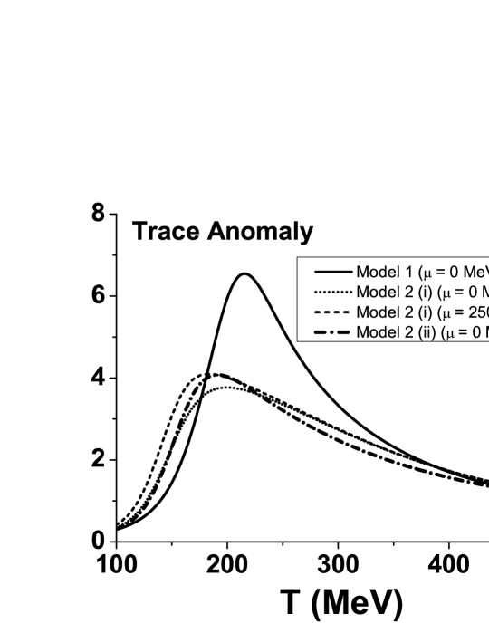
(a)

Figure 1: Trace anomaly for several chemical potentials.

III.3 Numerical Results

We start our numerical study following the calculations developed in raja , with no bulk effects and considering that the evolution starts at $\tau_{0}=0.5\,fm$, with $\Phi(\tau_{0})=0$. We want to compare different equations of state and determine the effects of certain features of these EOS (such as, for example, finite chemical potential) on the evolution of the fluid. To do this we would like to evolve them starting from the same initial state. However this is not possible because if they represent systems at the same initial temperature, then, these systems will have different initial energy densities and vice-versa. In relativistic heavy ion collisions, before thermal equilibrium formation, energy is released from the projectiles in a certain volume in the central rapidity region. It is perhaps more realistic to say that the quark-gluon system has first a defined energy density determined from the conditions of the collisions and then it reaches thermal equilibrium, forming a QGP with the properties determined by the equation of state. Since it is very difficult to know what comes first, energy density or temperature, we will test the two possibilities: same initial temperature, $T_{initial}=305\,MeV$ and same initial energy density, $\varepsilon_{initial}=16\,GeV/fm^{3}$. We will find out that our conclusions regarding cavitation do not depend on this choice and are the same for different initial conditions.

We solve the coupled equations (15) and (16) to obtain the temperature for each model considered. The temperature evolution at zero chemical potential is showed in Fig. 2.

(a)

(b)

Figure 2: Temperature evolution with no bulk effects for Model 1 and Model 2 (i) from $\tau_{0}=0.5\,fm$ to $\tau_{final}=10\,fm$ at zero chemical potential. a) Same initial temperature. b) Same initial energy density.

The effects of the chemical potential are presented in Fig. 3 for Model 2. From the figure we clearly see that systems with larger chemical potential cool faster.

(a)

(b)

Figure 3: Temperature evolution with no bulk effects for Model 2 (i) from $\tau_{0}=0.5\,fm$ to $\tau_{final}=10\,fm$ at finite chemical potential. a) Same initial temperature. b) Same initial energy density.

Cavitation is an effect mostly associated with peaks of the bulk viscosity close to phase transition raja ; romacav ; deni15 . We now consider bulk effects via eq. (17) with the relaxation scale approximated by $\tau^{\eta}_{\Pi}=\tau^{\zeta}_{\Pi}$. As previously mentioned, cavitation is generated when the longitudinal pressure, $P_{\xi}$, is negative and it starts when $P_{\xi}(\tau_{cav})=0$ in (14), where $\tau_{cav}$ is the time at which the longitudinal pressure vanishes. In this subsection we will make use of (7) to (11) to solve numerically the three coupled evolution equations (15), (16) and (17) and determine the time evolution of the longitudinal pressure (14).

We start with zero chemical potential in Fig. 4 for the two models with the initial conditions $\tau_{0}=0.5\,fm$, $\Phi(\tau_{0})=0$, $\Pi(\tau_{0})=0$ for $T_{initial}=305\,MeV$ and also for $\varepsilon_{initial}=16\,GeV/fm^{3}$.

(a)

(b)

Figure 4: Time evolution of the longitudinal pressure (14) from $\tau_{0}=0.5\,fm$ and zero chemical potential. See Tables 1 and 2. a) Same initial temperature. b) Same initial energy density.

Table 1: Time when cavitation starts (in Fig. 4(a) )

	$\tau_{cav}$ $[fm]$   (fixed $T_{initial}=305\,MeV$)
Model 1	2.3
Model 2 (i)	2.9

Table 2: Time when cavitation starts (in Fig. 4(b) )

	$\tau_{cav}$ $[fm]$   (fixed $\varepsilon_{initial}=16\,GeV/fm^{3}$)
Model 1	2.22
Model 2 (i)	4.06

In Fig. 5 we show results at finite chemical potentials for the Model 2. The cavitation starts earlier for increasing the chemical potential.

(a)

(b)

Figure 5: Time evolution of the longitudinal pressure (14) from $\tau_{0}=0.5\,fm$ and finite chemical potential for the Model 2. See Tables 3 and 4 for values of the chemical potential. a) Same initial temperature. b) Same initial energy density.

Table 3: Time when cavitation starts (in Fig. 5(a) )

	$\tau_{cav}$ $[fm]$   (fixed $T_{initial}=305\,MeV$)
Model 2 (i)  $(\mu=50\,MeV)$	2.91
Model 2 (i)  $(\mu=250\,MeV)$	2.84
Model 2 (i)  $(\mu=500\,MeV)$	2.63

Table 4: Time when cavitation starts (in Fig. 5(b) )

	$\tau_{cav}$ $[fm]$   (fixed $\varepsilon_{initial}=16\,GeV/fm^{3}$)
Model 2 (i)  $(\mu=50\,MeV)$	4.04
Model 2 (i)  $(\mu=250\,MeV)$	3.8
Model 2 (i)  $(\mu=500\,MeV)$	3.15

IV Cavitation in a non-conformal holographic plasma

One interesting question is whether it is possible to find cavitation within different approaches for the underlying many-body microscopic dynamics. From the strongly coupled nature of the QGP, in particular near the deconfinement transition temperature, the microscopic physics should be inherently non-perturbative. In this context, holographic methods may shed light upon the nature of transport coefficients for such strongly coupled plasmas, since these coefficients are difficult to obtain from lattice methods.

We follow the parametrization and second-order theory from hugo14 . Considering Bjorken symmetry and flat spacetime, our analysis reduces to solving the following dissipative equations:

$$\tau_{\Pi}^{\eta}\left(D\pi^{\langle\mu\nu\rangle}+\frac{4\theta}{3}\pi^{\mu\nu}\right)+\pi^{\mu\nu}=-2\eta\sigma^{\mu\nu}+\frac{\lambda_{1}}{\eta^{2}}\pi_{\lambda}^{\langle\mu}\pi^{\nu\rangle\lambda}+\tau_{\pi}^{*}\pi^{\mu\nu}\,\frac{\Pi}{3\zeta}\,$$ (26)

and

$$\tau_{\Pi}^{\zeta}\left(D\Pi+\Pi\theta\right)+\Pi=-\zeta\theta+\frac{\xi_{1}}{\eta^{2}}\pi_{\mu\nu}\pi^{\mu\nu}+\frac{\xi_{2}}{\zeta^{2}}\Pi^{2}+\tau_{\Pi}^{\zeta}\,\Pi\,\,D\ln\left(\frac{\zeta}{s}\right)\,.$$ (27)

The employed holographic method is a bottom-up solution gubser-nellore that parametrizes some of the thermodynamical properties of lattice (2+1)-flavor QCD near the crossover phase transition, described by Model 2 (ii) at zero chemical potential with the parameters ratti ; hugo14 . The trace anomaly with these parameters is shown in Fig. 1.

It is known that holographic calculations of transport coefficients, such as the holographic value of $\eta/s=1/4\pi$ kss , are generally consistent with experimental investigations of the evolution of QGP. The calculations employing usual kinetic theory result in larger values of $\eta/s$, which corroborates that holographic calculations are at least consistent with the QGP evolution near the deconfinement region depack .

The advantage of this approach is that the non-trivial temperature dependence of the transport coefficients were calculated for a phenomenological bottom-up model and parametrized in hugo14 . In the next subsection we summarize the relevant results.

IV.1 Transport coefficients and Bjorken flow

The coefficient $\eta/s$ is still $1/4\pi$, as is expected for several holographic models kss ; Buchel:2003tz . The shear relaxation time is parametrized as follows ($T_{c}^{h}=143.8$ MeV):

$$\frac{\tau_{\Pi}^{\eta}\,\eta}{T^{2}}\left(x=\frac{T}{T_{c}^{h}}\right)=\frac{a_{\eta}^{h}}{1+e^{b_{\eta}^{h}\left(c_{\eta}^{h}-x\right)}+e^{d_{\eta}^{h}\left(e_{\eta}^{h}-x\right)}+e^{f_{\eta}^{h}\left(g_{\eta}^{h}-x\right)}},$$ (28)

where $a_{\eta}^{h}$ to $g_{\eta}^{h}$ are fit parameters listed in Tab. 5.

The parametrization of bulk viscosity is:

$$\frac{\zeta}{s}\left(x=\frac{T}{T_{c}^{h}}\right)=\frac{a_{bulk}^{h}}{\sqrt{\left(x-b_{bulk}^{h}\right)^{2}+{(c_{bulk}^{h})}^{2}}}+\frac{d_{bulk}^{h}}{x^{2}+{(e_{bulk}^{h})}^{2}},$$ (29)

where $a_{bulk}^{h}$ to $e_{bulk}^{h}$ are fit parameters in Tab. 5.

In order to parametrize the bulk relaxation time, we adopt a causality bound, relating it to the shear relaxation time hugo14 :

$$\tau_{\Pi}^{\zeta}T\left(x=\frac{T}{T_{c}^{h}}\right)=\frac{a_{\zeta}^{h}}{\sqrt{\left(x-b_{\zeta}^{h}\right)^{2}+({c_{\zeta}^{h})}^{\,2}}}+\frac{d_{\zeta}^{h}}{x},$$ (30)

with the corresponding fit parameters $a_{\zeta}^{h}$ to $d_{\zeta}^{h}$ being given in Tab. 5.

Table 5: Parameters: $\tau_{\Pi}^{\eta}\,\eta/T^{2}$ for Eq. (28),
$\zeta/s$ for Eq. (29)  and   $\tau_{\Pi}^{\zeta}T$ for Eq. (30).

$a_{\eta}^{h}$	$b_{\eta}^{h}$	$c_{\eta}^{h}$	$d_{\eta}^{h}$	$e_{\eta}^{h}$	$f_{\eta}^{h}$	$g_{\eta}^{h}$
0.2664	2.029	0.7413	0.1717	-10.76	9.763	1.074
$a_{bulk}^{h}$	$b_{bulk}^{h}$	$c_{bulk}^{h}$	$d_{bulk}^{h}$	$e_{bulk}^{h}$
0.01162	1.104	0.2387	-0.1081	4.870
$a_{\zeta}^{h}$	$b_{\zeta}^{h}$	$c_{\zeta}^{h}$	$d_{\zeta}^{h}$
0.05298	1.131	0.3958	-0.05060

The other coefficients are determined in a phenomenological approach. However there is still a non-trivial behavior near the transition temperature. These are estimates considering fluid-gravity calculations for conformal fluid, as well as other strongly coupled holographic calculations Bhattacharyya:2008jc ; brsss ; Kanitscheider:2009as . We consider then the following hugo14 :

$$\lambda_{1}=\frac{2\eta^{2}}{sT}\,,$$

$$\tau_{\pi}^{*}=-3\tau_{\Pi}^{\eta}\left(\frac{1}{3}-c_{s}^{2}\right)\,,$$

$$\xi_{1}=\lambda_{1}\left(\frac{1}{3}-c_{s}^{2}\right)\,,$$

$$\xi_{2}=2\eta\tau_{\Pi}^{\zeta}\,c_{s}^{2}\left(\frac{1}{3}-c_{s}^{2}\right)\,.$$

In Fig. 6(a) we show the two bulk expressions given by (10) and (29) using the parametrizations from raja ; hugo14 ; deni15 . Notice that near the deconfinement temperature the bulk viscosity per entropy density of the holographic calculation given by (29) is significantly smaller than (10). Both come from distinct microscopic approaches and the difference between them reflects our lack of knowledge on the subject. We hope that future theoretical and experimental work can shed light upon bulk viscosity properties of strongly coupled plasmas. Similarly, in Fig. 6(b) we present the two relaxation times as a function of the temperature, (8) and (28). Eq.(8) is the result of a conformal calculation and Eq. (28) includes non-conformal contributions calculate through holography.

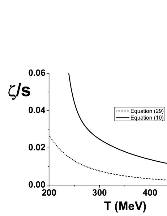
(a)

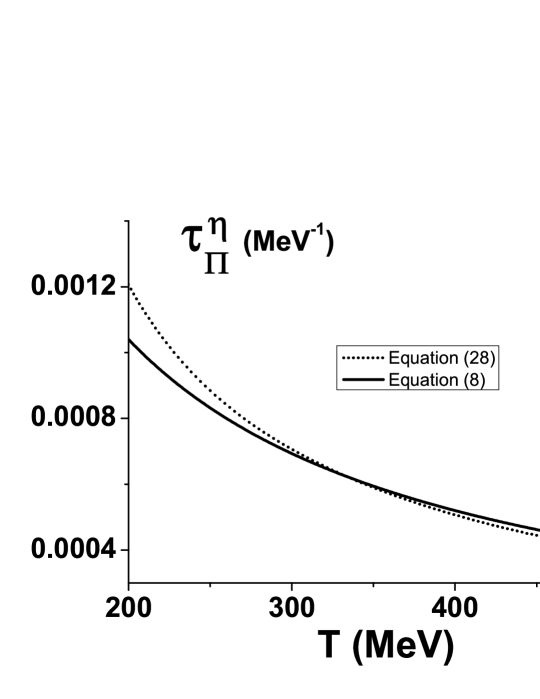
(b)

Figure 6: (a) Bulk per entropy density. (b) Relaxation scale. The parametrizations come from raja ; hugo14 ; deni15 .

It is straightforward to solve Eqs. (26) and (27) in the Bjorken flow. We follow the conventions adopted in the previous section, so the evolution equations are (15) and the following:

$$\tau^{\eta}_{\Pi}\frac{\partial\Phi}{\partial\tau}=\frac{4\eta}{3\tau}-\Phi-\left[\frac{4\tau^{\eta}_{\Pi}}{3\tau}\Phi+\frac{\lambda_{1}}{2\eta^{2}}\Phi^{2}\right]+\frac{\tau_{\pi}^{*}}{3\zeta}\Phi\Pi$$ (32)

and

$$\tau^{\zeta}_{\Pi}\frac{\partial\Pi}{\partial\tau}+\tau^{\zeta}_{\Pi}{\frac{\Pi}{\tau}}=-\frac{\zeta}{\tau}-\Pi+\frac{3}{2}\frac{\xi_{1}}{\eta^{2}}\Phi^{2}+\frac{\xi_{2}}{\zeta^{2}}\Pi^{2}+\frac{\tau_{\Pi}^{\zeta}}{(\zeta/s)}\Bigg{[}{\frac{\partial}{\partial T}}\left(\frac{\zeta}{s}\right)\Bigg{]}{\frac{\partial T}{\partial\tau}}\,.$$ (33)

In particular, equations (32) and (33) are the same as (16) and (17) but with extra transport coefficients. One interesting feature of such second order theory is that both bulk and shear evolution equations are nonlinear and coupled to each other. The entropy density in (29), (32) and (33) is calculated via (11) using the equation of state of the Model $2$.

We solve numerically Eqs. (15), (32) and (33) in the Bjorken flow and with the discussed holographic transport coefficients to search possible indications of cavitation. We consider the initial conditions $\tau_{0}=0.5\,fm$, $\Phi(\tau_{0})=0$, $\Pi(\tau_{0})=0$ for both initial approaches $T_{initial}=305\,MeV$ and also $\varepsilon_{initial}=16\,GeV/fm^{3}$.

(a)

(b)

Figure 7: (a) Temperature evolution for the non-conformal holographic QGP. (b) Time evolution of the longitudinal pressure (14) for the non-conformal holographic QGP at zero chemical potential.

As can be seen in Fig. 7 cavitation does not occur. It is often the case with holographic transport coefficients that dissipative effects seem to be smaller than others obtained from different methods, such as kinetic theory calculations. Nonetheless, the holographic values for small ratio of shear viscosity per entropy density are consistent so far with experimental results, and thus we suggest that, if confirmed by experimental data, the absence of cavitation may be a consequence of the strongly coupled nature of QGP.

In order to compare the Models $1$ and $2$ with the non-conformal holographic Model we show again, in Fig. 8 and in Fig. 9 the same plots of the temperature and longitudinal pressure evolution previously presented in Fig. 2, Fig. 4 and Fig. 7.

(a)

(b)

Figure 8: Temperature evolution with (a) same initial temperature and (b) same initial energy density.

(a)

(b)

Figure 9: Longitudinal pressure evolution with (a) same initial temperature and (b) same initial energy density.

V Conclusions

In this work, we considered several equations of state at different chemical potentials in order to investigate the occurrence of cavitation in QGP. This was done through a numerical integration of the Bjorken hydrodynamical equations and determination of the pressure as a function of proper time.

We used a phenomenological parametrization of the lattice QCD equation of state with two sets of transport coefficients. For the bulk viscosity we used a parametrization of results obtained in a Monte-Carlo simulation of pure gluon dynamics SU(3) meyer07 ; raja . For both lattice QCD and mean field QCD equations of state, cavitation occurs at smaller time scales as the chemical potential increases.

As is often the case with transport coefficients calculated with lattice methods near the phase transition, the height of the bulk per entropy density peak is not generally well established, most calculations rely on pure glue dynamics and consequently on the existence of first order phase transitions. We considered a phenomenological holographic calculation of transport coefficients of a non-conformal QGP hugo14 . In our approach, we conclude that cavitation does not occur in the holographic prescription, specially due to the small bulk viscosity as shown in Fig. 6(a) and by Eq. (29). Even with the addition of more transport coefficients (which contain peaks near the crossover phase transition) this approach does not support cavitation. In the future it may be possible to compare these distinct cavitation results in the scenario where lattice calculations of bulk effects can consistently consider the crossover phase transition. We hope that once the magnitude of bulk effects in the QGP is more precisely calculated, we can be more conclusive on whether cavitation occurs.

It should be interesting to generalize our calculations to more complex flows and check whether cavitation can be obtained in different regimes. Also, a non trivial check of the observable effects of cavitation in QGP would be the study of stability properties of hadron gas bubbles, as well as how their collapse influences the overall evolution of the plasma. We leave such investigations for future work.

- (1) K. Adcox et al. [PHENIX Collaboration], Nucl. Phys. A 757, 184 (2005)
- (2) J. Adams et al. [STAR Collaboration], Phys. Rev. Lett. 91, 172302 (2003)
- (3) K. Aamodt et al. [ALICE Collaboration], Phys. Rev. Lett. 105, 252301 (2010)
- (4) B. Muller, J. Schukraft and B. Wyslouch, Ann. Rev. Nucl. Part. Sci. 62, 361 (2012).
- (5) P. Romatschke, Int. J. Mod. Phys. E 19, 1 (2010).
- (6) U. Heinz and R. Snellings, Ann. Rev. Nucl. Part. Sci. 63, 123 (2013).
- (7) T. Schaefer and D. Teaney, Rept. Prog. Phys. 72, 126001 (2009).
- (8) C. Gale, S. Jeon, B. Schenke, P. Tribedy and R. Venugopalan, Phys. Rev. Lett. 110, 012302 (2013).
- (9) G. Torrieri, B. Tomasik and I. Mishustin, Phys. Rev. C 77, 034903 (2008).
- (10) G. Torrieri and I. Mishustin, Phys. Rev. C 78, 021901 (2008).
- (11) K. Rajagopal and N. Tripuraneni, JHEP 1003, 018 (2010).
- (12) C. E. Brennen, Cavitation and Bubble Dynamics, First Edition, Oxford University Press, 1995.
- (13) M. Habich and P. Romatschke, JHEP 1412, 054 (2014).
- (14) G. S. Denicol, S. Jeon and C. Gale, Phys. Rev. C 90, 024912 (2014); J. Noronha-Hostler, J. Noronha and F. Grassi, Phys. Rev. C 90, 034907 (2014); J. Noronha-Hostler, G. S. Denicol, J. Noronha, R. P. G. Andrade and F. Grassi, Phys. Rev. C 88, 044916 (2013); K. Dusling and T. Schafer, Phys. Rev. C 85, 044909 (2012); P. B. Arnold, C. Dogan and G. D. Moore, Phys. Rev. D 74, 085021 (2006).
- (15) W. Florkowski, R. Ryblewski, N. Su and K. Tywoniuk, arXiv:1504.03176 [hep-ph]; E. Lu and G. D. Moore, Phys. Rev. C 83, 044901 (2011); A. Dobado, F. J. Llanes-Estrada and J. M. Torres-Rincon, Phys. Lett. B 702, 43 (2011).
- (16) A. Andronic, Int. J. Mod. Phys. A 29, 1430047 (2014).
- (17) A. Dumitru, L. Portugal and D. Zschiesche, Phys. Rev. C 73, 024902 (2006).
- (18) S. Borsanyi, G. Endrodi, Z. Fodor, S. D. Katz, S. Krieg, C. Ratti and K. K. Szabo, JHEP 1208, 053 (2012); Y. Aoki, G. Endrodi, Z. Fodor, S. D. Katz and K. K. Szabo, Nature 443, 675 (2006).
- (19) S. Borsanyi, Z. Fodor, C. Hoelbling, S. D. Katz, S. Krieg and K. K. Szabo, Phys. Lett. B 730, 99 (2014).
- (20) S. I. Finazzo, R. Rougemont, H. Marrochio and J. Noronha, JHEP 1502, 051 (2015).
- (21) G. S. Denicol, C. Gale and S. Jeon, arXiv:1503.00531 [nucl-th].
- (22) D. A. Fogaça, H. Marrochio, F. S. Navarra and J. Noronha, Nucl. Phys. A 934, 18 (2014).
- (23) W. Israel, Annals Phys. 100, 310 (1976); W. Israel and J. M. Stewart, Annals Phys. 118, 341 (1979).
- (24) J. D. Bjorken, Phys. Rev. D 27, 140 (1983).
- (25) A. Muronga, Phys. Rev. C 69, 034903 (2004).
- (26) P. Kovtun, D. T. Son and A. O. Starinets, Phys. Rev. Lett. 94, 111601 (2005).
- (27) R. Baier, P. Romatschke, D. T. Son, A. O. Starinets and M. A. Stephanov, JHEP 04 (2008) 100.
- (28) A. Bazavov et al., Phys. Rev. D 80, 014504 (2009).
- (29) S. M. Sanches, F. S. Navarra and D. A. Fogaça, Nucl. Phys. A 937, 1 (2015).
- (30) S. S. Gubser and A. Nellore, Phys. Rev. D 78, 086007 (2008).
- (31) G. S. Denicol, T. Koide and D. H. Rischke, Phys. Rev. Lett. 105, 162501 (2010); G. S. Denicol, J. Noronha, H. Niemi and D. H. Rischke, Phys. Rev. D 83, 074019 (2011); G. S. Denicol, H. Niemi, E. Molnar and D. H. Rischke, Phys. Rev. D 85, 114047 (2012).
- (32) A. Buchel and J. T. Liu, Phys. Rev. Lett. 93, 090602 (2004).
- (33) S. Bhattacharyya, V. E. Hubeny, S. Minwalla and M. Rangamani, JHEP 0802, 045 (2008).
- (34) I. Kanitscheider and K. Skenderis, JHEP 0904, 062 (2009).
- (35) H. B. Meyer, Phys. Rev. Lett. 100, 162001 (2008).