Low-Rank Matrix Recovery from Row-and-Column Affine Measurements

Abstract

We propose and study a row-and-column affine measurement scheme for low-rank matrix recovery. Each measurement is a linear combination of elements in one row or one column of a matrix $X$. This setting arises naturally in applications from different domains. However, current algorithms developed for standard matrix recovery problems do not perform well in our case, hence the need for developing new algorithms and theory for our problem. We propose a simple algorithm for the problem based on Singular Value Decomposition ($SVD$) and least-squares ($LS$), which we term SVLS . We prove that (a simplified version of) our algorithm can recover $X$ exactly with the minimum possible number of measurements in the noiseless case. In the general noisy case, we prove performance guarantees on the reconstruction accuracy under the Frobenius norm. In simulations, our row-and-column design and SVLS algorithm show improved speed, and comparable and in some cases better accuracy compared to standard measurements designs and algorithms. Our theoretical and experimental results suggest that the proposed row-and-column affine measurements scheme, together with our recovery algorithm, may provide a powerful framework for affine matrix reconstruction.

Keywords: low-rank matrix recovery, row and column measurements, matrix completion, singular value decomposition

1 Introduction

In the low-rank affine matrix recovery problem, an unknown matrix $X\in\mathbb{R}_{n_{1}\times n_{2}}$ with $rank(X)=r$ is measured indirectly via an affine transformation $\mathcal{{A}}:\mathbb{R}_{n_{1}\times n_{2}}\rightarrow\mathbb{R}^{d}$ and possibly with additive (typically Gaussian) noise $z\in\mathbb{R}^{d}$. Our goal is to recover $X$ from the vector of noisy measurements $\mathbf{b}=\mathcal{{A}}(X)+z$. The problem has found numerous applications throughout science and engineering, in different fields such as collaborative filtering [19], face recognition [1], quantum state tomography [14] and computational biology [9]. The problem has been studied mathematically quite extensively in the last few years. Most attention thus far has been given to two particular ensembles of random transformations $\mathcal{{A}}$: (i) the Matrix Completion (MC) setting, in which each element of $\mathcal{{A}}(X)$ is a single entry of the matrix where the subset of the observed measurements is sampled uniformly at random [6, 4, 8, 17, 18, 21] (ii) Gaussian-Ensemble (GE) affine-matrix-recovery, in which each element of $\mathcal{{A}}(X)$ is a weighted sum of all elements of $X$ with i.i.d. Gaussian weights [5, 22]. Remarkably, although the recovery problem is in general NP-hard, when $r\ll min(n_{1},n_{2})$ and under certain conditions on the matrix $X$ or the measurement operator $\mathcal{{A}}$, one can recover $X$ from $d\ll n_{1}n_{2}$ measurements with high probability and using efficient algorithms [6, 22, 8, 21]. However, it is desirable to study the problem with other affine transformations $\mathcal{{A}}$ beyond the two ensembles mentioned above for the following reasons: (i) In some applications we cannot control the measurements operator $\mathcal{{A}}$, and different models for the measurements may be needed to allow a realistic analysis of the problem (ii) When we can control and design the measurement operator $\mathcal{{A}}$, other measurement operators may outperform the two ensembles mentioned above with respect to optimizing different resources such as the number of measurements required, computation time and storage. The main goal of this paper is to present and study a different set of affine transformations, which we term row-and-column affine measurements. This setting may arise naturally in many applications, since it is often natural and possibly cheap to measure a single row or column of a matrix, or a linear combination of a few such rows and columns. For example, (i) In collaborative filtering, we may wish to recover a users-items preference matrix and have access to only a subset of the users, but can observe their preference scores for all items (ii) When recovering a protein-RNA interactions matrix in molecular biology, a single experiment may simultaneously measure the interactions of a specific protein with all RNA molecules [10].

In general, we can represent any affine transformation $\mathcal{{A}}$ in matrix representation $\mathcal{{A}}(X)=Avec(X)$, where $vec(X)$ is a column vector obtained by stacking all columns of $X$ on top of each other. In our row and column framework the measurement operator $\mathcal{{A}}$ is represented differently using two matrices $A^{(R)},A^{(C)}$ which multiply $X$ as a matrix (rather than multiplying the vector $vec(X)$) from left and right, respectively. We focus on two ensembles of $A^{(R)},A^{(C)}$: (i) Matrix Completion from single Columns and Rows (RCMC). Here we observe single matrix entries in similar to standard matrix completion case, however the measured entries are not scattered randomly along the matrix, but instead we sample a few rows and a few columns, and measure all entries in these rows and columns. This ensemble is implemented by setting the rows (columns) of $A^{(R)}$ $(A^{(C)})$ as random vectors from the standard basis of $\mathbb{R}^{n_{1}}$ ($\mathbb{R}^{n_{2}}$). (ii) Gaussian Row-and-Column (GRC) measurements. Here each set of measurements is a weighted linear combination of the matrix’s rows (or columns) with the weights taken as i.i.d. Gaussians. This ensemble is implemented by setting the entries of $A^{(R)},A^{(C)}$ as i.i.d. Gaussian random variables.

The measurement operators $\mathcal{{A}}$ in our RCMC and GRC models do not satisfy standard requirements which hold for GE and MC. It is thus not surprising that algorithms such as nuclear norm minimization [22, 6], which succeed for the GE and MC models, fail in our case, and different algorithms and theory are required. However, the specific algebraic structure provided by the row-and-column measurements, allows us to derive efficient and simple algorithms, and to analyze their performance. In addition, we provide extensive simulation results, which demonstrate the improved accuracy and speed of our approach over existing measurement designs and algorithms. All of our algorithms and simulations are implemented in a Matlab software package available at
https://github.com/avishaiwa/SVLS.

1.1 Prior Work

Before giving a detailed derivation and analysis of our design and algorithms, we give an overview of existing designs and their properties. We concentrate on two properties: (i) storage required in order to represent the measurement operator, and (ii) measurement sparsity, defined as the sum over all measurements of the number of matrix entries participating in each measurement, that is $S(\mathcal{{A}})=||vec(A)||_{0}$. The latter property may be related to measurement costs, as well as to computational time.

In the Gaussian Ensemble model, the entries of the matrix $A$ in the matrix representation $\mathcal{{A}}(X)=Avec(X)$ are i.i.d. Gaussian random variables, $A_{ij}\sim N(0,1)$. For this ensemble, one can recover uniquely a low rank matrix $X$ with $O(r(n_{1}+n_{2}))$ noiseless measurements using nuclear norm minimization [22, 5] or other methods such as Singular Value Projection (SVP) [16], which is optimal up to constants. Recovery in this model is robust to noise, with only a small increase in number of measurements. The main disadvantage of this model is that the design requires $O(dn_{1}n_{2})$ storage space for ${A}$, which could be problematic for large matrices. Another possible disadvantage of this method is that measurements are dense - each measurement represents a linear combination of all $O(n_{1}n_{2})$ matrix entries, and the overall measurement sparsity of $\mathcal{{A}}(X)$ is also $O(dn_{1}n_{2})$, which could be problematic for large $n_{1},n_{2}$.

In the standard matrix completion problem [6] we can recover $X$ with high probability from single entries chosen uniformly at random using nuclear norm minimization [2, 26, 8, 20, 21] or using other methods such as $SVD$ and gradient descent [17, 18]. This model has the lowest storage requirements ($O(d)$) and measurement sparsity ($O(d)$). However, recovery guarantees for this model are weaker: setting $n=\max(n_{1},n_{2})$, it is shown that $\Theta(nrlog(n))$ measurements are required to recover a rank $r$ matrix of size $n_{1}\times n_{2}$ [8]. In addition, unique recovery from this number of measurements requires additional incoherence conditions on the matrix $X$, and recovery of matrices which fail to satisfy such conditions (e.g. matrices with a few spikes) may require a much larger number of measurements.

Recently a new design of rank one projections was proposed [3], where each measurement is of the form $\alpha^{T}X\beta$ and such that $\alpha\in\mathbb{R}^{n_{1}},\beta\in\mathbb{R}^{n_{2}}$ have i.i.d standard Gaussian entries. It was proven that nuclear norm minimization can recover $X$ with high probability in this design from $O(n_{1}r+n_{2}r)$ measurements. This is the first model deviating from MC and GE we are aware of. This model is different from our row-and-column model, as each measurement is obtained by multiplying $X$ from both sides, whereas in our model each measurement is obtained by multiplying $X$ from either left or right. Moreover, in our model the measurements are not chosen independently from each other but come in groups of size $n_{1}$ or $n_{2}$ (corresponding to rows or columns $A^{(R)},A^{(C)}$). An advantage of rank one projection is that it leads to a significance reduction in measurement storage needed for $\mathcal{{A}}$ with overall $O(dn_{1}+dn_{2})$ storage space. However, each measurement is still dense and involve all matrix elements, hence measurement sparsity is $O(dn_{1}n_{2})$. In contrast, our $GRC$ model requires only $O(d)$ storage for $\mathcal{{A}}$, and every measurement depends only on $O(n)$ elements, leading to a reduced overall time for all measurements $O(dn_{1}+dn_{2})$. For RCMC, we need only $O(\frac{dlog(n)}{n})$ storage for $\mathcal{{A}}$, and measurement sparsity is $O(d)$.

2 Preliminaries and Notations

We denote by $\mathbb{{R}}_{n_{1}\times n_{2}}$ the space of matrices of size $n_{1}\times n_{2}$, by $\mathcal{O}_{n_{1}\times n_{2}}$ the space of matrices of size $n_{1}\times n_{2}$ with orthonormal columns, and by $\mathcal{{M}}_{n_{1}\times n_{2}}^{(r)}$ the space of matrices of size $n_{1}\times n_{2}$ and rank $\leqslant r$. We denote $n=\max(n_{1},n_{2})$.

We denote by $||\cdot||_{F}$ the matrix Frobenius norm, by $||\cdot||_{*}$ the nuclear norm, and by $||\cdot||_{2}$ the spectral norm. For a vector, $||\cdot||$ denotes the standard $l_{2}$ norm.

For $X\in\mathbb{{R}}_{n_{1}\times n_{2}}$we denote by $span(X)$ the subspace of $\mathbb{R}^{n_{1}}$ spanned by the columns of $X$ and define $P_{X}$ to be the orthogonal projection into $span(X)$.

For a matrix $X$ we denote by $X_{i\bullet}$ the $i$-th row, by $X_{\bullet j}$ the $j$-th column and by $X_{ij}$ the $(i,j)$ element. For two sets of indices $I,J$, we denote by $X_{IJ}$ the sub-matrix obtained by taking the rows with indices in $I$ and columns with indices in $J$ of $X$. We denote by $[k]$ the set of indices $1,..,k$. We denote by $vec(X)$ the (column) vector obtained by stacking all the columns of $X$ on top of each other.

We use the notation $X\overset{i.i.d.}{\sim}G$ to denote a random matrix $X$ with i.i.d. entries $X_{ij}\sim G$.

For a rank-$r$ matrix $X\in\mathcal{{M}}_{n_{1}\times n_{2}}^{(r)}$ let $X=U\Sigma V^{T}$ be the Singular Value Decomposition ($SVD$) where $U\in\mathcal{O}_{n_{1}\times r},\thinspace V\in\mathcal{O}_{r\times n_{2}}$ and $\Sigma=diag(\sigma_{1}(X),...,\sigma_{r}(X))$ with $\sigma_{1}(X)\geq\sigma_{2}(X)\geq..\geq\sigma_{r}(X)>0$ the (non-zero) singular values of $X$ (we omit the zero singular values and their corresponding vectors from the decomposition). For a general matrix $X\in\mathbb{{R}}_{n_{1}\times n_{2}}$ we denote by $X_{(r)}$ the top-$r$ singular value decomposition of $X$, $X_{(r)}=U_{\bullet[r]}\Sigma_{[r][r]}V_{\bullet[r]}^{T}$.

Our model assumes two affine transformations applied to $X$, representing rows and columns, $B^{(C,0)}=XA^{(C)}$ and $B^{(R,0)}=A^{(R)}X,$ achieved by multiplications with two matrices $A^{(R)}\in\mathbb{{R}}_{k^{(R)}\times n_{1}}$ and $A^{(C)}\in\mathbb{{R}}_{n_{2}\times k^{(C)}}$, respectively. We obtain noisy observations of these transformations, $B^{(R)},B^{(C)}$ obtained by applying additive noise:

$$A^{(R)}X+Z^{(R)}=B^{(R)}\,;\quad XA^{(C)}+Z^{(C)}=B^{(C)}$$ (1)

where the total number of measurements is $d=k^{(R)}n_{1}+n_{2}k^{(C)}$, and $Z^{(R)}\in\mathbb{R}_{n_{1}\times k^{(R)}}$,$Z^{(C)}\in\mathbb{R}_{k^{(C)}\times n_{2}}$ are two zero-mean noise matrices. Our goal is to recover $X$ from the observed measurements $B^{(C)}$ and $B^{(R)}$. To achieve this goal, we define the squared loss function

$$\mathcal{\mathcal{\mathcal{{F}}}}(X)=||A^{(R)}X-B^{(R)}||_{F}^{2}+||XA^{(C)}-B^{(C)}||_{F}^{2}$$ (2)

and solve the least squares problem:

$$Minimize\>\mathcal{\mathcal{{F}}}(X)\>s.t.\>X\in\mathcal{{M}}_{n_{1}\times n_{2}}^{(r)}.$$ (3)

If $Z^{(R)},Z^{(C)}\overset{i.i.d.}{\sim}N(0,\tau^{2})$ , minimizing the loss function in eq. (2) is equivalent to maximizing the log-likelihood of the data, giving a statistical motivation for the above score. Problem (3) is non-convex due to the non-convex rank constraint $rank(X)\leq r$.

Our problem is a specialization of the general affine matrix recovery problem [22], in which a matrix is measured using a general affine transformation $\mathcal{{A}}$ with $\mathbf{b}=\mathcal{{A}}(X)+z$. We consider next and throughout the paper two specific random ensembles of measurement matrices:

1. Row and Column Matrix Completion (RCMC): In this ensemble each row of $A^{(R)}$ and each column of $A^{(C)}$ is a vector of the standard basis $e_{j}$ for some $j$ - thus each measurement $B^{(R)}_{ij}$ or $B^{(C)}_{ij}$is obtained from a single entry of $X$. We define a row-inclusion probability $p^{(R)}$ and column inclusion probability $p^{(C)}$ such that each row (column) of $X$ will be measured with probability $p^{(R)}$ ($p^{(C)}$). More precisely, we define $r_{1},..,r_{n_{1}}$ i.i.d. Bernoulli variables, $P(r_{i}=1)=p^{(R)}$, and include $e_{i}$ as a row in $A^{(R)}$ if and only if $r_{i}=1$. Similarly, we define $c_{1}...c_{n_{2}}$ i.i.d. Bernoulli variables, $P(c_{i}=1)=p^{(C)}$, and include $e_{i}$ as a column in $A^{(C)}$ if and only if $c_{i}=1$. The expected number of observed rows (columns) is $k^{(R)}=n_{1}p^{(R)}$ ($k^{(C)}=n_{2}p^{(C)}$). The model is very similar to the possibly more natural model of picking $k^{(R)}$ distinct rows and $k^{(C)}$ distinct columns at random for fixed $k^{(R)},k^{(C)}$, but allows for easier analysis.

2. Gaussian Rows and Columns (GRC): In this ensemble $A^{(R)},A^{(C)}\overset{i.i.d.}{\sim}N(0,1)$. Each observation $B^{(R)}_{ij}$ or $B^{(C)}_{ij}$ is obtained by a weighted sum of a single row or column of $X$, with i.i.d. Gaussian weights.

2.1 Comparison to Standard Designs

Our proposed rows-and-columns design differs from standard designs appearing in the literature. It is instructive to compare our GRC ensemble to the Gaussian Ensemble (GE) [5], with the matrix representation $\mathcal{{A}}(X)=Avec(X)$ where $A\in\mathbb{{R}}_{d\times n_{1}n_{2}}$ and $A\overset{i.i.d.}{\sim}N(0,1)$. For the latter, the following $r$-Restricted Isometry Property (RIP) can be used:

Definition 1.

(r-RIP) Let $\mathcal{{A}}:\mathbb{{R}}_{n_{1}\times n_{2}}\rightarrow\mathbb{R}^{d}$ be a linear map. For every integer $r$ with $1\leq r\leq min(n_{1},n_{2})$, define the $r$-Restricted Isometry Constant to be the smallest number $\epsilon_{r}$ such that

$$(1-\epsilon_{r})||X||_{F}\leq||\mathcal{{A}}(X)||\leq(1+\epsilon_{r})||X||_{F}$$ (4)

holds for all matrices $X$ of rank at most $r$.

The GE model satisfies the $r$-RIP condition for $d=O(rn)$ with high probability [22]. Based on this property it is known that nuclear norm minimization [22, 5] and other algorithms such as SVP [16] can recover $X$ with high probability. Unlike GE, in our GRC model $\mathcal{{A}}(X)$ doesn’t satisfy the $r$-RIP, and nuclear norm minimization fails. Instead, $A^{(R)},A^{(C)}$ preserve matrix Frobenius norm in high probability - a weaker property which holds for any low-rank matrix. (see Lemma 7 in the Appendix).

We next compare RCMC to the standard Matrix Completion model [6], in which single entries are chosen at random to be observed. Unlike GE, for MC incoherence conditions on $X$ are required in order to guarantee unique recovery of $X$ [6] :

Definition 2.

(Incoherence). Let $U$ be a subspace of $\mathbb{R}^{n}$ of dimension $r$, and $P_{U}$ be the orthogonal projection on $U$. Then the coherence of $U$ (with respect to the standard basis $\{e_{i}\}$) is defined as

$$\text{$\mu$}(U)\text{$\equiv$}\frac{n}{r}max_{i}||P_{U}(e_{i})||^{2}.$$ (5)

We say that a matrix $X\in\mathbb{{R}}_{n_{1}\times n_{2}}$ is $\mu$-incoherent if for the $SVD$ $X=U\Sigma V^{T}$ we have $max(\mu(U),\mu(V))\leq\mbox{$\mu$}$.

When $X$ is $\mu$-incoherent, and when known entries are sampled uniformly at random from $X$, several algorithms [17, 2, 16] succeed to recover $X$ with high probability. In particular, nuclear norm minimization has gained popularity as a solver for the standard MC problem because it provides recovery guarantees and a convenient representation as a convex optimization problem with availability of many iterative solvers for the problem. However, nuclear norm minimization fails for the RCMC design, even when the matrix $X$ is incoherent, as shown by the next example:

Example 1.

Take $X\in\mathbb{{R}}_{n\times n}$ for $\frac{n}{3}\in\mathbb{N}$ with $X_{ij}=1,\>\>\forall(i,j)\in[n]\times[n]$. Thus $||X||_{*}=n$. Take $k^{(R)}=k^{(C)}=\frac{n}{3}$. Set all unknown entries to $0.5$, giving a matrix $X_{0}$ of rank $2$ with $\sigma_{1}(X_{0})=\frac{(\sqrt{2}+1)n}{3}$, $\sigma_{2}(X_{0})=\frac{(\sqrt{2}-1)n}{3}$. Therefore $||X_{0}||_{*}=\frac{n\sqrt{2}}{3}<||X||_{*}$ and nuclear norm minimization fails to recover the correct $X$.

In Section 3 we present our SVLS algorithm, which does not rely on nuclear-norm minimization. In Section 4 we show that SVLS successfully approximates $X$ for the GRC ensemble.

3 Algorithms for Recovery of $X$

In this section we give an efficient algorithm which we call SVLS (Singular Value Least Squares). SVLS is very easy to implement - for simplicity, we start with Algorithm 1 for the noiseless case and then present Algorithm 2 (SVLS ​) which is applicable for the general (noisy) case.

3.1 Noiseless Case

In the noiseless case we reduce the optimization problem (3) to solving a system of linear equations [6], and provide Algorithm 1, which often leads to a closed-form estimator. We then give conditions under which with high probability, the closed-form solution is unique and is equal to the true matrix $X$.

Input: $A^{(R)},A^{(C)},B^{(R)},B^{(C)}$ and rank $r$

1. Compute a basis (of size $r$) to the column space of $B^{(C)}$ using Gaussian elimination, represented as the columns of a matrix $\hat{U}\in\mathbb{{R}}_{n_{1}\times r}$.

2. Solve the linear system $B_{\bullet j}^{(R)}=A^{(R)}\hat{U}Y_{\bullet j}$ for each $j=1,..,n_{2}$ and write the solutions as a matrix $Y=Y_{\bullet 1}...Y_{\bullet n_{2}}$.

3. Output $\hat{X}=\hat{U}Y$

Algorithm 1

If $rank(A^{(R)}\hat{U})=r$ one can write the resulting estimator $\hat{X}$ in closed-form as follows:

$$\hat{X}=\hat{U}Y=\hat{U}[\hat{U}^{T}A^{(R)^{T}}A^{(R)}\hat{U}]^{-1}\hat{U}^{T}A^{(R)^{T}}B^{(R)}$$ (6)

Algorithm 1 does not treat the row and column measurements symmetrically. We can apply the same algorithm, but changing the role of rows and columns. The resulting closed form solution is then:

$$\hat{X}=B^{(C)}A^{(C)}\hat{V}[\hat{V}^{T}A^{(C)}A^{(C)^{T}}\hat{V}]^{-1}\hat{V}^{T}$$ (7)

for an orthogonal matrix $\hat{V}$ representing a basis for the rows of $X$. Since the algorithm uses Gaussian elimination steps for solving systems of linear equations, it is crucial that we have exact noiseless measurements. Next, we modify the algorithm to work also for noisy measurements.

3.2 General (Noisy) Case

In the noisy case we seek a matrix $X$ minimizing the loss $\mathcal{\mathcal{{F}}}$ in eq. (2). The minimization problem is non-convex and there is no known algorithm with optimality guarantees. We propose Algorithm 2 (SVLS ​), which empirically returns a matrix estimator $\hat{X}$ with a low value of the loss $\mathcal{\mathcal{{F}}}$. In addition, we prove in Section 4 recovery guarantees on the performance of SVLS ​.

Input: $A^{(R)},A^{(C)},B^{(R)},B^{(C)}$ and rank $r$

1. Compute $\hat{U}$, the $r$ largest left singular vectors of $B^{(C)}$, ($\hat{U}$ is a basis for the columns space of $B^{(C)}_{(r)}$).

2. Find the least-squares solution

   $$\hat{Y}=argmin_{Y}\parallel B^{(R)}-A^{(R)}\hat{U}Y||_{F}.$$ (8)

   If $rank(A^{(R)}\hat{U})=r$ we can write $\hat{Y}$ in closed form as before:

   $$\hat{Y}=[\hat{U}^{T}A^{(R)^{T}}A^{(R)}\hat{U}]^{-1}\hat{U}^{T}A^{(R)^{T}}B^{(R)}.$$ (9)

3. Compute the estimate $\hat{X}^{(R)}=\hat{U}\hat{Y}$.

4. Repeat steps 1-3, replacing the roles of columns and rows to get an estimate $\hat{X}^{(C)}$.

5. Set $\hat{X}=argmin_{\hat{X}^{(R)},\hat{X}^{(C)}}\mathcal{\mathcal{{F}}}(X)$, for the loss $\mathcal{\mathcal{{F}}}(X)$ given in eq. (2).

Algorithm 2 SVLS

3.2.1 Gradient Descent

The estimator $\hat{X}$ returned by SVLS may not minimize the loss function $\mathcal{\mathcal{{F}}}$ in eq. (2). We therefore perform an additional gradient descent stage starting from $\hat{X}$ to achieve an estimator with lower loss (while still possibly only a local minimum since the problem is non-convex). SVLS can be thus viewed as a fast method for providing a desirable starting point for local-search algorithms. The details of the gradient descent are given in the Appendix, Section 7.2.

3.3 Estimation of Unknown Rank

In real life problems, one doesn’t know the true rank of a matrix and should estimate it from data. Our rows-and-columns sampling design is particularly suitable for rank estimation since $rank(B^{(C,0)})=rank(B^{(R,0)})=rank(X)$ with high probability when enough rows and columns are sampled. In the noiseless case we can estimate $rank(X)$ by $\hat{r}$=$rank(B^{(C,0)})$ or $rank(B^{(R,0)})$.

For the noisy case we estimate $rank(X)$ from $B^{(C)},B^{(R)}$. We use the popular elbow method to estimate $rank(B^{(C)})$ in the following way

$$\hat{r}^{(C)}=argmax_{i\in[k^{(C)}-1]}\left(\frac{\sigma_{i}(B^{(C)})}{\sigma_{i+1}(B^{(C)})}\right)$$ (10)

We compute similarly $\hat{r}^{(R)}$ from $B^{(R)}$ and take the average as our rank estimator, $\hat{r}=round\left(\frac{\hat{r}^{(C)}+\hat{r}^{(C)}}{2}\right)$. We demonstrate the performance of our rank estimation using simulations in the Appendix, Section 7.7.

Modern methods for rank estimation from singular values [13] can be similarly applied to $B^{(R)},B^{(C)}$ and may yield more accurate rank estimates. After we estimate the rank, we can plug-in $\hat{r}$ as the rank parameter in the SVLS algorithm and recover $X$.

3.4 Low Rank Approximation

In the low rank matrix approximation problem, the goal is to approximate a (possibly full rank) matrix $X$ by the closest (in Frobenius norm) rank-$r$ matrix $X_{(r)}$. By the Eckart-Young Theorem [12], this problem has a closed-form solution which is the truncated $SVD$ of $X$. $SVD$ is a powerful tool in affine matrix recovery and different algorithms such as SVT, OptSpace , SVP and others apply $SVD$. In [15] the authors try to find a low rank approximation to $X$ using measurements $X{A^{(C)}}=B^{(C)}$ and ${A^{(R)}}X=B^{(R)}$. For large $n_{1},n_{2}$ they give a single-pass algorithm which computes $X_{(r)}$ using only $B^{(C)}$ and $B^{(R)}$. We bring their algorithm in the Appendix, Section 7.6. The main difference between the above formulation and our problem in eq. (3) is the rank estimation. In [15] it is assumed that $k^{(R)}=k^{(C)}=k$ and one estimates $X_{(k)}$ instead of a rank-$r$ matrix which can lead to poor performance if $r\ll k$. We adjusted the algorithm presented in [15] to our problem and give a new estimator which is a combination of SVLS and [15]’s method, replacing $\hat{X}^{(R)}$ and $\hat{X}^{(C)}$ in steps 3,4 of SVLS by:

$$\quad\hat{X}^{(R)}_{P}=\hat{X}^{(R)}\hat{V}\hat{V}^{T}\>,\quad\hat{X}^{(C)}_{P}=\hat{U}\hat{U}^{T}\hat{X}^{(C)}.$$ (11)

Here $\hat{V}$ is the $r$ largest right singular vectors of $B^{(R)}$ and $\hat{U}$ is the $r$ largest left singular vectors of $B^{(C)}$. We call this new estimator $SVLS_{P}$. Simulations show almost identical and in some cases slightly better performance of this modified algorithm compared to SVLS (see Appendix, Section 7.6). This modified estimator is however difficult to analyze rigorously, and therefore we present throughout the paper our results for the SVLS estimator.

4 Performance Guarantees

In this section we give guarantees on the accuracy of the estimator $\hat{X}$ returned by SVLS ​. Our guarantees are probabilistic, with respect to randomizing the design matrices $A^{(R)},A^{(C)}$. For the noiseless case we give conditions which are close to optimal for exact recovery.

4.1 Noiseless Case

A rank $r$ matrix of size $n_{1}\times n_{2}$ has $r(n_{1}+n_{2}-r)$ degrees of freedom, and can therefore not be uniquely recovered by fewer measurements. Setting $k^{(R)}=k^{(C)}=r$ gives precisely this minimal number of measurements. We next show that this number suffices, with probability $1$, to guarantee accurate recovery of $X$ in the GRC model. In the RCMC model the number of measurements is increased by a logarithmic factor in $n$ and we need an additional incoherence assumption on $X$ in order to guarantee accurate recovery with high probability. We first present two Lemmas which will be useful. Their proofs are given in the Appendix, Section 7.

Lemma 1.

Let $X_{1},X_{2}\in\mathcal{{M}}_{n_{1}\times n_{2}}^{(r)}$ and $A^{(R)}\in\mathbb{{R}}_{k^{(R)}\times n_{1}},A^{(C)}\in\mathbb{{R}}_{n_{2}\times k^{(C)}}$ such that $rank(A^{(R)}X_{1})=rank(X_{1}A^{(C)})=r$. If $A^{(R)}X_{1}=A^{(R)}X_{2}$ and $X_{1}A^{(C)}=X_{2}A^{(C)}$ then $X_{1}=X_{2}$.

Lemma 2.

Let $X\in\mathcal{{M}}_{n_{1}\times n_{2}}^{(r)}$ and $A^{(R)}\in\mathbb{{R}}_{k^{(R)}\times n_{1}},A^{(C)}\in\mathbb{{R}}_{n_{2}\times k^{(C)}}$ such that $rank(A^{(R)}X)=rank(XA^{(C)})=r$. For Algorithm 1 with inputs $A^{(R)},A^{(C)},B^{(R,0)},$ $B^{(C,0)}$ and $r$ the output $\hat{X}$ satisfies

$$A^{(R)}X=A^{(R)}\hat{X},\,XA^{(C)}=\hat{X}A^{(C)}$$ (12)

4.1.1 Exact Recovery for GRC

For the noiseless case, we can recover $X$ with the minimal number of measurements, as shown in Theorem 1 (proof given in the Appendix, Section 7):

Theorem 1.

Let $\hat{X}$ be the output of Algorithm 1 in the GRC model with $Z^{(C)},Z^{(R)}=0$ and $k^{(R)},k^{(C)}\geq r$. Then $P(\hat{X}=X)=1$.

4.1.2 Exact Recovery for RCMC

In the RCMC model, rows and columns of $X$ are sampled with replacement. Since the same row can be sampled over and over, we cannot guarantee uniqueness of solution, as was the case for the GRC model, but rather wish to prove that exact recovery of $X$ is possible with high probability. We assume the Bernoulli rows and columns model as described in Section 2 and assume for simplicity that $k^{(R)}=k^{(C)}=k$.

Theorem 2.

Let $X=U\Sigma V^{T}$ be the $SVD$ of $X\in\mathbb{{R}}_{n_{1}\times n_{2}}$, and $\max(\mu(U),\mu(V))<\mu$. Take $A^{(R)}$ and $A^{(C)}$ as in the RCMC model without noise and probabilities $p^{(R)}=\frac{k}{n_{1}}$ and $p^{(C)}=\frac{k}{n_{2}}$. Let $\beta>1$ such that $C_{R}\sqrt{\frac{\beta log(n)r\mu}{k}}<1$ where $C_{R}$ is uniform constant and let $\hat{X}$ be the output of Algorithm 1. Then $P\left(\hat{X}=X\right)>1-6min(n_{1},n_{2})^{-\beta}$.

The proof of Theorem 2 is in the Appendix, Section 7.

Remark 1.

Both row and column measurements are need in order to guarantee unique recovery. If, for example, we observe only rows then even with $n-1$ observed rows and rank $r=1$ we can only determine the unobserved row up to a constant, and thus cannot recover $X$ uniquely.

4.2 General (Noisy) Case

In the noisy case we cannot guarantee exact recovery of $X$, and our goal is to minimize the error $||X-\hat{X}||_{F}$ for $\hat{X}$ the output of SVLS ​. Here, we give bounds on the error for the GRC model. For simplicity, we show the result for $k^{(R)}=k^{(C)}=k$.

We focus on the high dimensional case $k\leq n$, where the number of measurements is low. In this case our bound is similar to the bound of the Gaussian Ensemble (GE). In [5] it is shown for GE that $||X-\hat{X}||_{F}<C_{G}\sqrt{\frac{nr\tau^{2}}{d}}$ holds with high probability for some constant $C_{G}$. We next give an analogous result for our GRC model (proof in the Appendix, Section 7.4).

Theorem 3.

Let $A^{(R)}$ and $A^{(C)}$ with $k\geq max(4r,40)$ be as in the GRC model with noise matrices $Z^{(R)},Z^{(C)}$. Let $\hat{X}$ be the output of SVLS. Then there exist constants $c,c^{(R)},c^{(C)}$ such that with probability $>1-5e^{-ck}$:

$$||X-\hat{X}||_{F}\leq\sqrt{\frac{r}{k}}\Big{[}c^{(C)}||Z^{(C)}||_{2}+c^{(R)}||Z^{(R)}||_{2}\Big{]}.$$ (13)

Theorem 3 applies for any $Z^{(C)}$ and $Z^{(R)}$. If $k\leq n$ and $Z^{(R)},Z^{(C)}\overset{i.i.d.}{\sim}N(0,\tau^{2})$, then from eq. (35) we get $max(||Z^{(R)}||_{2},||Z^{(C)}||_{2})\leq 4\tau\sqrt{n}$ with probability $1-e^{-2n}$. We therefore get the next Corollary for i.i.d. additive Gaussian noise:

Corollary 1.

Let $A^{(R)}$, $A^{(C)}$ as in the GRC with $n\geq k\geq max(4r,40)$, model and $Z^{(R)},Z^{(C)}\overset{i.i.d.}{\sim}N(0,\tau^{2})$. Then there exist constants $c,C_{GRC}$ such that:

$$P\Big{(}||X-\hat{X}||_{F}\leq C_{GRC}\sqrt{\frac{\tau^{2}nr}{k}}\Big{)}>1-5e^{-ck}-e^{-2n}.$$ (14)

5 Simulations Results

We studied the performance of our algorithm using simulations. We measured the reconstruction accuracy using the Relative Root-Mean-Squared-Error ($RRMSE$), defined as

$$RRMSE\equiv RRMSE(X,\hat{X})\equiv||X-\hat{X}||_{F}/||X||_{F}.$$ (15)

For simplicity, we concentrated on square matrices with $n_{1}=n_{2}=n$ and used an equal number of row and column measurements, $k^{(R)}=k^{(C)}=k$ . In all simulations we sampled a random rank-$r$ matrix $X=UV^{T}$ with $U,V\in\mathbb{{R}}_{n\times r}$ , $U,V\overset{i.i.d.}{\sim}N(0,\sigma^{2})$.

In all simulations we assumed that $rank(X)$ is unknown and estimated using the elbow method in eq. (10).

5.1 Row-Column Matrix Completion (RCMC)

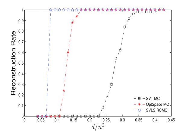
In the noiseless case we compared our design to standard MC. We compared the reconstruction rate (probability of exact recovery of $X$ as function of the number of measurements $d$) for the RCMC design with SVLS to the reconstruction rate for the standard MC design with the OptSpace [18] and SVT[2] algorithms. To allow for numerical errors, for each simulation yielding $X$ and $\hat{X}$ we defined recovery as successful if their $RRMSE$ was lower than $10^{-3}$, and for each value of $d$ recorded the percentage of simulations for which recovery was successful. In Figure 1 we show results for $n=150,r=3$ and $\sigma=1$. SVLS recovers $X$ with probability $1$ with the optimal number of measurements $d=r(2n-r)=894$ yielding $\frac{d}{n^{2}}\approx 0.04$ while MC with OptSpace and SVT need roughly $3$-fold and $8$-fold more measurements, respectively, to guarantee exact recovery.

Figure 1: Reconstruction rates for matrices with dimension $n=150$ and $r=3$ where $d$ is the number of known entries varied between $0$ to $8000$. SVT and OptSpace are applied to the standard MC design and Algorithm 1 to RCMC. For each $d$ we sampled $50$ matrices and calculated the reconstruction rate as described in the main text.

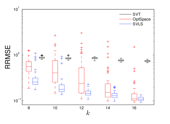
The improvement in accuracy is not due to our design or our algorithm alone, but due to their combination. We compared our method to OptSpace and SVT for RCMC. We sampled a matrix $X$ with $n=100,r=3,\sigma=1$ and noise level $\tau^{2}=0.25^{2}$, and varied the number of row and column measurements $k$. Figure 2 shows that while the performance of SVLS is very stable even for small $k$, the performance of OptSpace varies, with multiple instances achieving poor accuracy, and SVT which minimizes the nuclear norm achieves poor accuracy for all problem instances.

Remark 2.

The OptSpace algorithm has a trimming step which delete dense columns. We omitted this step in the RCMC model since it would delete all the known columns and rows and it’s not stable for this type of measurements, but it still get better result than SVT.

Figure 2: Box-plots represent the distribution of $RRMSE$ as a function of the number of column and row measurements $k$ over $50$ different sampled matrices $X=UV^{T}$ with $U,V\overset{i.i.d.}{\sim}N(0,1)$ and $Z^{(R)},Z^{(C)}\overset{i.i.d.}{\sim}N(0,0.25^{2})$. OptSpace (red) fails to recover $X$ on many instances while SVLS (blue) performs very well on all of them. SVT (black) fails to recover $X$ for all instances. The trimming of dense rows and columns in OptSpace was skipped, since such trimming in our settings may delete all measurement information for low $k$.

Next, we compared our RCMC to standard MC. We sampled $X$ as before with $U,V\in\mathbb{R}_{1000\times r}$ with standard Gaussian distribution, different rank and different noise ratio. The observations were corrupted by additive Gaussian noise $Z$ with relative noise level $NR\equiv||Z||_{F}/||X||_{F}$.

Results, displayed in Table 1, show that SVLS is significantly faster than the other two algorithms. It is also more accurate than MC for small number of measurements, and comparable to MC for large number of measurements.

NR	$d$	$r$	SVLS	OptSpace	SVT
​$10^{-2}\!\!\!$	$120156$​	​$10$​	​$0.0063$ $(0.15)$​	​$0.004$ $(20.8)$​	​$0.0073$ $(18.7)$​
​$10^{-1}\!\!\!$	$120156$​	​$10$​	​$0.064$ $(0.15)$​	​$0.044$ $(21.7)$​	​$0.05$ $(11)$​
​$1\!\!\!$	$120156$​	​$10$​	​$0.612$ $(0.16)$​	​$0.49$ $(24.5)$​	​$0.51$ $(1)$​
​$10^{-2}\!\!\!$	$59100$​	​$20$​	​$0.029$ $(0.12)$​	​$0.97$ $(25.6)$​	​$0.76$ $(4.4)$​
​$10^{-1}\!\!\!$	$59100$​	​$20$​	​$0.3$ $(0.12)$​	​$0.98$ $(40.1)$​	​$0.86$ $(6.5)$​
​$10^{-1}\!\!\!$	$391600$​	​$50$​	​$0.081$ $(0.7)$​	​$0.05$ $(1200)$​	​$0.069$ $(13)$​
​$1\!\!\!$	$391600$​	​$50$​	​$0.72$ $(0.6)$​	​$0.61$ $(1300)$​	​$0.59$ $(5)$​

Table 1: $RRMSE$ and time in seconds (in parenthesis) for SVLS applied to RCMC, and OptSpace and SVT applied to the standard MC. Results represent average of $5$ different random matrices. SVLS is faster than OptSpace and SVT by 1 to 3 orders of magnitudes, and shows comparable or better $RRMSE$ in all cases.

Finally, we checked for RCMC and MC our performance only on unobserved entries, to examine if $RRMSE$ is optimistic due to overfitting to observed entries. Results, shown in the Appendix, Section 7.8, indicate than no overfitting is observed.

5.2 Gaussian Rows and Columns (GRC)

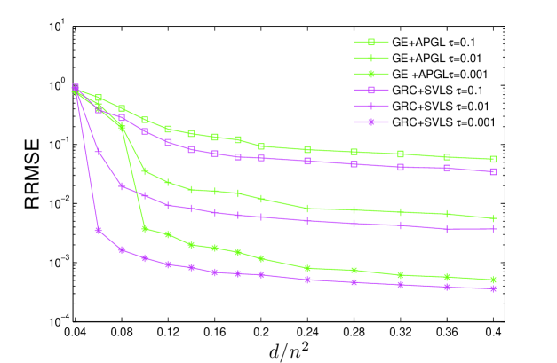
We tested the performance of the GRC model with $A^{(R)},A^{(C)}\overset{i.i.d.}{\sim}N(0,\frac{1}{n})$ and with $X=UV^{T}$ where $U,V\overset{i.i.d.}{\sim}N(0,\frac{1}{\sqrt{r}})$. We compare our results to the Gaussian Ensemble model (GE) where for each $n$, $\mathcal{{A}}(X)$ was normalized to allow a fair comparison. In Figure 3 we take $n=100$ and $r=2$, and change the number of measurements $d=2nk$ (where $A^{(R)}\in\mathbb{R}_{k\times n}$ and $A^{(C)}\in\mathbb{R}_{n\times k}$). We added Gaussian noise $Z^{(R)},Z^{(C)}$ with different noise levels $\tau$. For all noise levels, the performance of GRC was better than the performance of GE. The $RRMSE$ error decays at a rate of $\sqrt{k}$. For GE we used the APGL algorithm [26] for nuclear norm minimization.

Figure 3: $RRMSE$ as function of $d$, the number of measurements, where we take $X\in\mathcal{{M}}_{100\times 100}^{(2)}$, $d$ is varied from $400$ to $4000$ and for different noise levels: $\tau=0.1,0.01$ and $0.001$. For every point we simulated $5$ random matrices and computed the average $RRMSE$.

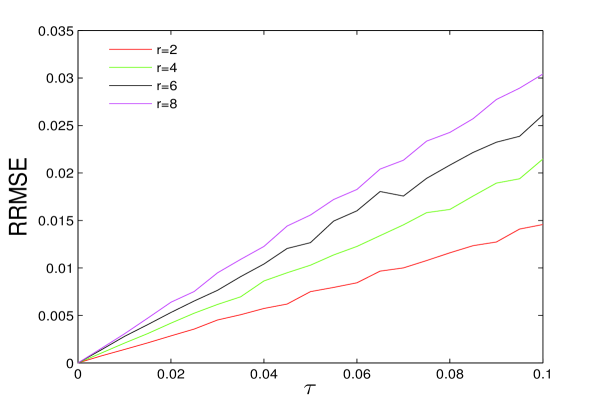
In the next tests we ran SVLS for measurements with different noise levels. We take $n=1000$ and $k=100$ with different rank level every entry in $Z^{(C)},Z^{(R)}\overset{i.i.d.}{\sim}N(0,\tau^{2})$ and different values of $\tau$. Results are shown in Figure 4. The change in the relative error $RRMSE$ is linear in $\tau$ while the rate depends on $r$.

We next examined the behaviour of the $RRMSE$ when $n\to\infty$ and when $n,k,r\rightarrow\infty$ together, while the ratios $\frac{k}{n}$ and $\frac{d}{r}$ are kept constant. Results (shown in the Appendix, Section 7.5) indicate that when properly scaled, the $RRMSE$ error is not sensitive to the value of $n$ and other parameters, in agreement with Theorem 3.

6 Discussion

We introduced a new measurements ensemble for low rank matrix recovery where every measurements is an affine combination of a row or column of $X$. We focused on two models: matrix completion from single columns and rows (RCMC) and matrix recovery from Gaussian combination of columns and rows (GRC). We proposed a fast algorithm for this ensemble. For the RCMC model we proved that in the noiseless case our method recovers $X$ with high probability and simulation results show that the RCMC model outperforms the standard approach for matrix completion in both speed and accuracy for models with small noise.

Figure 4: $RRMSE$ as a function of noise level $\tau$ varied from $0$ to $0.1$, for matrices $X\in\mathbb{{R}}_{1000\times 1000}$ of different ranks. For each curve we fitted a linear regression line, with fitted slopes $0.145,0.208,0.25,0.3$ for $r=2,4,6,8$, respectively. The slope is roughly proportional to $\sqrt{r}$ in concordance with the error bound in Theorem 3. Further investigation of the relation using extensive simulations is required in order to evaluate the dependency of the recovery error in $r$ in a more precise manner.

For the GRC model we proved that our method recovers $X$ with the optimal number of measurements in the noiseless case and gave an upper bounds on the error for the noisy case. For RCMC, our simulations show that the RCMC design may achieve comparable or favorable results, compared to the standard MC design, especially for low noise level. Proving recovery guarantees for this RCMC model is an interesting future challenge.

Our proposed measurement scheme is not restricted to recovery of low-rank matrices. One can employ this measurement scheme and recover $X$ by minimizing other matrix norms. This direction can lead to new algorithms that may improve matrix recovery for real datasets.

7 Appendix

7.1 Proofs for Noiseless GRC Case

Proof of Lemma 1

Proof.

First, $rank(X_{2}A^{(C)})=rank(X_{1}A^{(C)})=r$ and similarly $rank(A^{(R)}X_{2})=\allowbreak rank(A^{(R)}X_{1})\allowbreak=\allowbreak r$. Since $span(X_{1}A^{(C)}),span(X_{2}A^{(C)})$ are subspaces of $span(X_{1}),\allowbreak span(X_{2})$ respectively, and $dim(span(X_{2}))\leq r$ we get $span(X_{2})=span(X_{2}A^{(C)})\allowbreak=span(X_{1}A^{(C)})=span(X_{1})$, and we define $U\in\mathcal{O}_{n_{1}\times r}$ a basis for this subspace. For $X_{1},X_{2}$ there are $Y_{1},Y_{2}\in\mathbb{{R}}_{r\times n_{2}}$ such that $X_{1}=UY_{1},X_{2}=UY_{2}$. Therefore $A^{(R)}UY_{1}=A^{(R)}UY_{2}$. Since $rank(A^{(R)}UY_{1})=r$ and $U\in\mathcal{O}_{n_{1}\times r}$ we get $rank(A^{(R)}U)=r$, hence the matrix $U^{T}A^{(R)^{T}}A^{(R)}U$ is invertible, which gives $Y_{1}=Y_{2}$, and therefore $X_{1}=UY_{1}=UY_{2}=X_{2}$.  

Proof of Lemma 2

Proof.

$span(XA^{(C)})\subseteq span(X)$ and $rank(XA^{(C)})=rank(X)=r$, therefore $span(XA^{(C)})=span(X)$ and $\hat{U}$ from stage 1 in Algorithm 1 is a basis for $span(X)$. We can write $X=\hat{U}Y$ for some matrix $Y\in\mathbb{R}_{r\times n_{2}}$. Since $rank(A^{(R)}\hat{U}Y)=rank(\hat{U})=r$, we have $rank(A^{(R)}\hat{U})=r$. Thus eq. (6) gives $\hat{X}$ in closed form and we get:

$$A^{(R)}\hat{X}=A^{(R)}\hat{U}[\hat{U}^{T}A^{(R)^{T}}A^{(R)}\hat{U}]^{-1}\hat{U}^{T}A^{(R)^{T}}B^{(R,0)}=$$

$$A^{(R)}\hat{U}[\hat{U}^{T}A^{(R)^{T}}A^{(R)}\hat{U}]^{-1}\hat{U}^{T}A^{(R)^{T}}A^{(R)}\hat{U}Y=$$

$$A^{(R)}\hat{U}Y=A^{(R)}X.$$ (16)

$$\hat{X}A^{(C)}=\hat{U}[\hat{U}^{T}A^{(R)^{T}}A^{(R)}\hat{U}]^{-1}\hat{U}^{T}A^{(R)^{T}}A^{(R)}XA^{(C)}=$$

$$\hat{U}[\hat{U}^{T}A^{(R)^{T}}A^{(R)}\hat{U}]^{-1}\hat{U}^{T}A^{(R)^{T}}A^{(R)}\hat{U}YA^{(C)}=$$

$$\hat{U}YA^{(C)}=XA^{(C)}.$$ (17)

 

Lemma 3.

Let $V\in\mathcal{O}_{n\times r}$ and $A^{(C)}\in\mathbb{{R}}_{n\times k}$ be a random matrix $A^{(C)}\overset{i.i.d.}{\sim}N(0,\sigma^{2})$. Then $V^{T}A^{(C)}\overset{i.i.d.}{\sim}N(0,\sigma^{2})$.

Proof.

For any two matrices $A\in\mathbb{{R}}_{n_{1}\times n_{2}}$ and $B\in\mathbb{{R}}_{m_{1}\times m_{2}}$ we define their Kronecker product as a matrix in $\mathbb{{R}}_{n_{1}m_{1}\times n_{2}m_{2}}$:

$$A\otimes B=\left(\begin{array}[]{ccccc}a_{11}B&a_{12}B&.&.&a_{1n_{2}}B\\ .&.&.&.&.\\ .&.&.&.&.\\ .&.&.&.&.\\ a_{n_{1}1}B&a_{n_{1}2}B&.&.&a_{n_{1}n_{2}}B\\ \end{array}\right)$$ (18)

Now, we have $vec(V^{T}A^{(C)})=(I_{n}\otimes V^{T})vec(A^{(C)})$ and since $vec(A^{(C)})\sim N(0,\sigma I_{n})$ the vector $(I_{n}\otimes V^{T})vec(A^{(C)})$ is also a multivariate Gaussian vector with zero mean and covariance matrix:

$$COV\Big{(}V^{T}A^{(C)}\Big{)}=COV\Big{(}(I_{n}\otimes V^{T})vec(A^{(C)})\Big{)}=$$

$$(I_{n}\otimes V^{T})COV\left(vec(A^{(C)})\right)(I_{n}\otimes V^{T})^{T}=$$

$$\sigma^{2}(I_{n}\otimes V^{T})(I_{n}\otimes V^{T})^{T}=\sigma^{2}I_{r}\otimes I_{n}=\sigma^{2}I_{nr}.$$ (19)

 

Proof of Theorem 1

For the GRC model, Lemmas 1,2 and 3 can be used to prove exact recovery of $X$ with the minimal possible number of measurements:

Proof.

Let $U\Sigma V^{T}$ be the $SVD$ of $X$. From Lemma 3 the elements of the matrix $V^{T}A^{(C)}$ have a continuous Gaussian distribution and since the measure of low rank matrices is zero and $k^{(C)}\geq r$ we get that $P(rank(V^{T}A^{(C)})=r)=1$. Since $B^{(C)}=U\Sigma V^{T}A^{(C)}$ we get $P(rank(B^{(C)})=rank(U\Sigma V^{T}A^{(C)})=r)=1$. In the same way $P(rank(B^{(R)})=r)=1$. Combining Lemma 2 with Lemma 1 give us the required result.  

7.2 Gradient Descent

The gradient descent stage is performed directly in the space of rank $r$ matrices, using the decomposition $\hat{X}$=$WS$ where $W\in\mathbb{{R}}_{n_{1}\times r}$ and $S\in\mathbb{{R}}_{r\times n_{2}}$ and computing the gradient of the loss as a function of $W$ and $S$,

$$\mathcal{\mathcal{{L}}}(W,S)=\mathcal{\mathcal{{F}}}(WS)=||A^{(R)}WS-B^{(R)}||_{F}^{2}+||WSA^{(C)}-B^{(C)}||_{F}^{2}.$$ (20)

We want to minimize eq. (20) but the loss $\mathcal{\mathcal{{L}}}$ isn’t convex and therefore gradient descent may fail to converge to a global optimum. We propose $\hat{X}$ (the output of SVLS ​) as a starting point which may be close enough to enable gradient descent to converge to the global optimum, and in addition may accelerate convergence.

The gradient of $\mathcal{\mathcal{{L}}}$ is (using the chain rule)

$$\frac{\partial\mathcal{\mathcal{{L}}}}{\partial W}=2\Big{[}A^{(R)^{T}}(A^{(R)}WS-B^{(R)})S^{T}+(WSA^{(C)}-B^{(C)})A^{(C)^{T}}S^{T}\Big{]}$$

$$\frac{\partial\mathcal{\mathcal{{L}}}}{\partial S}=2\Big{[}W^{T}A^{(R)^{T}}(A^{(R)}WS-B^{(R)})+W^{T}(WSA^{(C)}-B^{(C)})A^{(C)^{T}}\Big{]}$$ (21)

7.3 Proofs for Noiseless RCMC Case

We prove that if $U\in\mathcal{O}_{n_{1}\times r}$ is orthonormal then with high probability we have $p^{-1}||U^{T}A^{(R)^{T}}A^{(R)}U-pI_{r}||_{2}<1$. Because $U$ is orthonormal, this is equivalent to

$$p{-1}||UU^{T}A^{(R)^{T}}A^{(R)}UU^{T}-pUU^{T}||_{2}<1\Leftrightarrow p^{-1}||P_{U}P_{A^{(R)^{T}}}P_{U}-pP_{U}||_{2}<1$$ (22)

where $P_{U}=UU^{T},P_{A^{(R)^{T}}}=A^{(R)^{T}}A^{(R)}$ and $p^{(R)}=p$. We generalize Theorem 4.1 from [6].

Lemma 4.

Suppose $A^{(R)}$ as in the RCMC model with inclusion probability $p$, and $U\in\mathcal{O}_{n_{1}\times r}$ with $\mu(U)=\frac{n_{1}}{r}max_{i}||P_{U}(e_{i})||^{2}=\mu$. Then there is a numerical constant $C_{R}$ such that for all $\beta>1$, if $C_{R}\sqrt{\frac{\beta log(n_{1})r\mu}{pn_{1}}}<1$ then:

$$P\left(p^{-1}||P_{U}P_{A^{(R)^{T}}}P_{U}-pP_{U}||_{2}<C_{R}\sqrt{\frac{\beta log(n_{1})r\mu}{pn_{1}}}\right)>1-3n_{1}^{-\beta}$$ (23)

The proof of Lemma 4 builds upon (yet generalizes) the proof of Theorem 4.1 from [6]. We next present a few lemmas which are required for the proof of Lemma 4. We start with a lemma from [7].

Lemma 5.

If $y_{i}$ is a family of vectors in $\mathbb{R}^{d}$ and ${r_{i}}$ is a sequence of i.i.d. Bernoulli random variables with $P(r_{i}=1)=p$, then

$$E\big{(}p^{-1}||\Sigma_{i}(r_{i}-p)y_{i}\otimes y_{i}||\big{)}<C\sqrt{\frac{log(d)}{p}}max_{i}||y_{i}||$$ (24)

for some numerical constant $C$ provided that the right hand side is less than $1$.

We next use a result from large deviations theory [25]:

Theorem 4.

Let $Y_{1}...Y_{n}$ be a sequence of independent random variables taking values in a Banach space and define

$$Z=sup_{f\in F}\sum_{i=1}^{n}f(Y_{i})$$ (25)

where $F$ is a real countable set of functions such that if $f\in F$ then $-f\in F$.

Assume that $|f|\leq B$ and $E(f(Y_{i}))=0$ for every $f\in F$ and $i\in[n]$. Then there exists a constant $C$ such that for every $t\geq 0$

$$P\big{(}|Z-E(Z)|\geq t\big{)}\leq 3exp\left(\frac{-t}{CB}log(1+\frac{t}{\sigma+Br})\right)$$ (26)

where $\sigma=sup_{f\in F}\sum_{i=1}^{n}E(f^{2}(Y_{i}))$.

Theorem 4 is used in the proof of the next lemma which is taken from Theorem 4.2 in [6]. We bring here the lemma and proof in our notations for convenience.

Lemma 6.

Let $U\in\mathcal{O}_{n\times r}$ with incoherence constant $\mu$. Let $r_{i}$ be i.i.d. Bernoulli random variables with $P(r_{i}=1)=p$ and let $Y_{i}=p^{-1}(r_{i}-p)P_{U}(e_{i})\otimes P_{U}(e_{i})$ for $i=1,..,n$. Let $Y=\sum_{i=1}^{n}Y_{i}$ and $Z=||Y||_{2}$. Suppose $E(Z)\leq 1$. Then for every $\lambda>0$ we have

$$P\Big{(}|Z-E(Z)|\geq\lambda\sqrt{\frac{\mu rlog(n)}{pn}}\Big{)}\leq 3exp\Big{(}-\gamma min(\lambda^{2}log(n),\lambda\sqrt{\frac{pnlog(n)}{\mu r}})\Big{)}$$ (27)

for some positive constant $\gamma$.

Proof.

We know that $Z=||Y||_{2}=sup_{f_{1},f_{2}}\langle f_{1},Yf_{2}\rangle=sup_{f_{1},f_{2}}\sum_{i=1}^{n}\langle f_{1,}Y_{i}f_{2}\rangle$, where the supremum is taken over a countable set of unit vectors $f_{1},f_{2}\in F_{V}$. Let $F$ be the set of all functions $f$ such that $f(Y)=\langle f_{1},Yf_{2}\rangle$ for some unit vectors $f_{1},f_{2}\in F_{V}$. For every $f\in F$ and $i\in[n]$ we have $E(f(Y_{i}))=0$. From the incoherence of $U$ we conclude that

$$|f(Y_{i})|=p^{-1}|r_{i}-p|\times|\langle f_{1},P_{U}(e_{i})\rangle|\times|\langle P_{U}(e_{i}),f_{2}\rangle|\leq p^{-1}||P_{U}(e_{i})||^{2}\leq p^{-1}\frac{r}{n}\mu.$$ (28)

In addition

$$E(f^{2}(Y_{i}))=p^{-1}(1-p)\langle f_{1},P_{U}(e_{i})\rangle^{2}\langle P_{U}(e_{i}),f_{2}\rangle^{2}\leq$$

$$p^{-1}||P_{U}(e_{i})||^{2}|\langle P_{U}(e_{i}),f_{2}\rangle^{2}|\leq p^{-1}\frac{r}{n}\mu|\langle P_{U}(e_{i}),f_{2}\rangle|^{2}.$$ (29)

Since $\sum_{i=1}^{n}|\langle P_{U}(e_{i}),f_{2}\rangle|^{2}=\sum_{i=1}^{n}|\langle e_{i},P_{U}(f_{2})\rangle|^{2}=||P_{U}(f_{2})||^{2}\leq 1$, we get $\sum_{i=1}^{n}E(f^{2}(Y_{i}))\leq p^{-1}\frac{r}{n}\mu.$

We can take $B=2p^{-1}\frac{r}{n}\mu$ and $t=\lambda\sqrt{\frac{\mu rlog(n)}{pn}}$ and from Theorem 4:

$$P(|Z-E(Z)|\geq t)\leq 3exp\left(\frac{-t}{KB}log(1+\frac{t}{2})\right)\leq 3exp\left(\frac{-tlog(2)}{KB}min(1,\frac{t}{2})\right)$$ (30)

where the last inequality is due to the fact that for every $u>0$ we have $log(1+u)\geq log(2)min(1,u)$. Taking $\gamma=-log(2)/K$ finishes our proof.  

We are now ready to prove Lemma 4

Proof.

(Lemma 4) Represent any vector $w\in R^{n_{1}}$ in the standard basis as $w=\sum_{i=1}^{n_{1}}\langle w,e_{i}\rangle e_{i}$. Therefore $P_{U}(w)=\sum_{i=1}^{n_{1}}\langle P_{U}(w),e_{i}\rangle e_{i}=\sum_{i=1}^{n_{1}}\langle w,P_{U}(e_{i})\rangle e_{i}$. Recall the $r_{i}$ Bernoulli variables which determine if $e_{i}$ is included as a row of $A^{(R)}$ as in Section 2 and define $Y_{i}$ and $Z$ as in Lemma 6. We get

$$P_{A^{(R)^{T}}}P_{U}(w)=\sum_{i=1}^{n_{1}}r_{i}\langle w,P_{U}(e_{i})\rangle e_{i}\Longrightarrow$$

$$P_{U}P_{A^{(R)^{T}}}P_{U}(w)=\sum_{i=1}^{n_{1}}r_{i}\langle w,P_{U}(e_{i})\rangle P_{U}(e_{i})$$ (31)

In other words the matrix $P_{U}P_{A^{(R)^{T}}}P_{U}$ is given by

$$P_{U}P_{A^{(R)^{T}}}P_{U}=\sum_{i=1}^{n_{1}}r_{i}P_{U}(e_{i})\otimes P_{U}(e_{i})$$ (32)

$U$ is $\mu-$incoherent, thus $max_{i\in[n_{1}]}||P_{U}(e_{i})||\leq\sqrt{\frac{\text{r}\mu}{n_{1}}}$, hence from Lemma 5 we have for $p$ large enough:

$$E({p}^{-1}||P_{U}P_{A^{(R)^{T}}}P_{U}-pP_{U}||_{2})<C\sqrt{\frac{log(n_{1})r\mu}{pn_{1}}}\leq 1.$$ (33)

For $\beta>1$ which satisfy the lemma’s requirement, take $\lambda=\sqrt{\frac{\beta}{\gamma}}$ where $\gamma$ as in Theorem 4. We get that if $p>\frac{\mu log(n_{1})r\beta}{n_{1}\gamma}$ then from Lemma 6 with probability of at least $1-3n_{1}^{-\beta}$ we have $Z\leq C\sqrt{\frac{log(n_{1})r\mu}{pn_{1}}}+\frac{1}{\sqrt{\gamma}}\sqrt{\frac{log(n_{1})r\mu\beta}{pn_{1}}}$. Taking $C_{R}=C+\frac{1}{\sqrt{\gamma}}$ finishes our proof.  

Proof of Theorem 2

Proof.

From Lemma 4 and using a union bound we have that with probability $>1-6min(n_{1},n_{2})^{-\beta}$, ${p^{(R)}}^{-1}||p^{(R)}I_{r}-U^{T}A^{(R)^{T}}A^{(R)}U||_{2}<1$ and ${p^{(C)}}^{-1}||p^{(C)}I_{r}-V^{T}A^{(C)}A^{(C)^{T}}V||_{2}<1$. Since the singular values of $p^{(R)}I_{r}-U^{T}A^{(R)^{T}}A^{(R)}U$ are $|p^{(R)}-\sigma_{i}(U^{T}A^{(R)^{T}}A^{(R)}U)|$ for $1\leq i\leq r$, we have

$$p^{(R)}-\sigma_{r}(U^{T}A^{(R)^{T}}A^{(R)}U)\leq\sigma_{1}(p^{(R)}I_{r}-U^{T}A^{(R)^{T}}A^{(R)}U)<p^{(R)}$$

$$\Rightarrow 0<\sigma_{r}(U^{T}A^{(R)^{T}}A^{(R)}U)$$ (34)

and similarly for $V^{T}A^{(C)}A^{(C)^{T}}V$. Therefore $rank(A^{(R)}U)=rank(V^{T}A^{(C)})=r$ and $rank(A^{(R)}X)=rank(XA^{(C)})=r$ with probability $>1-6min(n_{1},n_{2})^{-\beta}$. From Lemma 2 we get $A^{(R)}X=A^{(R)}\hat{X}\,\quad XA^{(C)}=\hat{X}A^{(C)}$ and from Lemma 1 we get $X=\hat{X}$ with probability $>1-6min(n_{1},n_{2})^{-\beta}$.  

7.4 Proofs for Noisy GRC Case

The proof of Theorem 3 is using strong concentration results on the largest and smallest singular values of $n\times k$ matrix with i.i.d Gaussian entries:

Theorem 5.

[24] Let $A\in\mathbb{{R}}_{n\times k}$ be a random matrix $A\overset{i.i.d.}{\sim}N(0,\frac{1}{n})$. Then, its largest and smallest singular values obey:

$$P\Big{(}\sigma_{1}(A)>1+\frac{\sqrt{k}}{\sqrt{n}}+t\Big{)}\text{$\leq$}e^{-nt^{2}/2}$$

$$P\Big{(}\sigma_{k}(A)\leq 1-\frac{\sqrt{k}}{\sqrt{n}}-t\Big{)}\text{$\leq$}e^{-nt^{2}/2}.$$ (35)

Corollary 2.

Let $A\in\mathbb{{R}}_{n\times k}$ be a random matrix $A\overset{i.i.d.}{\sim}N(0,1)$ where $n\geq 4k$, and let ${A}^{\dagger}$ be the Moore-Penrose pseudoinverse of $A$. Then

$$P\left(||{A}^{\dagger}||_{2}\leq\frac{6}{\sqrt{n}}\right)>1-e^{-n/18}$$ (36)

Proof.

Since ${A}^{\dagger}$ is the pseudoinverse of $A$, $||{A}^{\dagger}||_{2}$=$\frac{1}{\sigma_{k}(A)}$ and from Theorem 5 we get $\sigma_{k}(A)\geq\sqrt{n}-\sqrt{k}-t\sqrt{n}$ with probability $\geq 1-e^{nt^{2}/2}$ (notice the scaling by $\sqrt{n}$ of the entries of $A$ compared to Theorem 5). Therefore, if we take $n\geq 4k$ and $t=\frac{1}{3}$ we get

$$P\left(||{A}^{\dagger}||_{2}\leq\frac{6}{\sqrt{n}}\right)=P\left(\sigma_{k}(A)\geq\frac{\sqrt{n}}{6}\right)\geq 1-e^{-n/18}.$$ (37)

 

We also use the following lemma from [23]:

Lemma 7.

Let $Q$ to be a finite set of vectors in $\mathbb{R}^{n}$, let $\delta\in(0,1)$ and $k$ be an integer such that

$$\epsilon\equiv\sqrt{\frac{6log(2|Q|/\delta)}{k}}\leq 3.$$ (38)

Let $A\in\mathbb{{R}}_{k\times n}$ be a random matrix with $A\overset{i.i.d.}{\sim}N(0,\frac{1}{k})$. Then,

$$P\left(max_{x\in Q}\left|\frac{||Ax||^{2}}{||x||^{2}}-1\right|\leq\epsilon\right)>1-\delta.$$ (39)

Lemma 7 is a direct result of the Johnson-Lindenstrauss lemma [11] applied to each vector in $Q$ and using the union bound. Representing the vectors in $Q$ as a matrix, Lemma 7 shows that $A^{(R)},A^{(C)}$ preserve matrix Frobenius norm with high probability - a weaker property than the RIP which holds for any low-rank matrix.

To prove Theorem 3, we first represent $||X-\hat{X}||_{F}$ as a sum three parts (Lemma 8), then give probabilistic upper bounds to each of the parts and finally use union bound. We define $A_{\hat{U}}^{(R)}=A^{(R)}\hat{U}$ and $A_{V^{T}}^{(C)}=V^{T}A^{(C)}$. From Lemma 3 $A_{\hat{U}}^{(R)},A_{V^{T}}^{(C)}\overset{i.i.d.}{\sim}N(0,1)$, hence $rank(A_{\hat{U}}^{(R)})=rank(A_{V^{T}}^{(C)})=r$ with probability $1$. We assume w.l.o.g that $\hat{X}=\hat{X}^{(R)}$ (see SVLS description). Therefore, from eq. (9) we have $\hat{X}=\hat{U}(A_{\hat{U}}^{(R)^{T}}A_{\hat{U}}^{(R)})^{-1}A_{\hat{U}}^{(R)^{T}}B^{(R)}$.

We denote by ${A_{\hat{U}}^{(R)}}^{\dagger}=(A_{\hat{U}}^{(R)^{T}}A_{\hat{U}}^{(R)})^{-1}A_{\hat{U}}^{(R)^{T}}$and ${A_{V^{T}}^{(C)}}^{\dagger}=A_{V^{T}}^{(C)^{T}}(A_{V^{T}}^{(C)}A_{V^{T}}^{(C)^{T}})^{-1}$ the Moore-Penrose pseudoinverse of $A_{\hat{U}}^{(R)}$ and $A_{V^{T}}^{(C)}$, respectively. We next prove the following lemma

Lemma 8.

Let $A^{(R)}$ and $A^{(C)}$ be as in the GRC model and $Z^{(R)},Z^{(C)}$ be noise matrices. Let $\hat{X}$ be the output of SVLS ​. Then:

$$||X-\hat{X}||_{F}\leq\mathbf{I+II+III}$$

where:

$$\mathbf{I}\equiv||(B^{(C,0)}-B^{(C)}_{(r)}){A_{V^{T}}^{(C)}}^{\dagger}||_{F}$$ (40)

$$\mathbf{II\equiv}||\hat{U}{A_{\hat{U}}^{(R)}}^{\dagger}A^{(R)}(B^{(C,0)}-B^{(C)}_{(r)}){A_{V^{T}}^{(C)}}^{\dagger}||_{F}$$ (41)

$$\mathbf{III\equiv}||\hat{U}{A_{\hat{U}}^{(R)}}^{\dagger}Z^{(R)}||_{F}.$$ (42)

Proof.

We represent $||X-\hat{X}||_{F}$ as follows

$$||X-\hat{X}||_{F}=$$

$$||X-\hat{U}(A_{\hat{U}}^{(R)^{T}}A_{\hat{U}}^{(R)})^{-1}A_{\hat{U}}^{(R)^{T}}(A^{(R)}X+Z^{(R)})||_{F}=$$

$$||X-\hat{U}{A_{\hat{U}}^{(R)}}^{\dagger}A^{(R)}X\>-\hat{U}{A_{\hat{U}}^{(R)}}^{\dagger}Z^{(R)}||_{F}\leq$$

$$||X-\hat{U}{A_{\hat{U}}^{(R)}}^{\dagger}A^{(R)}X||_{F}+\mathbf{III}$$ (43)

where we have used the triangle inequality. We next use the following equality

$$XA^{(C)}{A_{V^{T}}^{(C)}}^{\dagger}V^{T}=U\Sigma V^{T}A^{(C)}{A_{V^{T}}^{(C)}}^{\dagger}V^{T}=U\Sigma V^{T}=X$$ (44)

to obtain:

$$||X-\hat{U}{A_{\hat{U}}^{(R)}}^{\dagger}A^{(R)}X||_{F}=$$

$$||(I_{n}-\hat{U}{A_{\hat{U}}^{(R)}}^{\dagger}A^{(R)})X||_{F}=$$

$$||(I_{n}-\hat{U}{A_{\hat{U}}^{(R)}}^{\dagger}A^{(R)})XA^{(C)}{A_{V^{T}}^{(C)}}^{\dagger}V^{T}||_{F}=$$

$$||(I_{n}-\hat{U}{A_{\hat{U}}^{(R)}}^{\dagger}A^{(R)})B^{(C,0)}{A_{V^{T}}^{(C)}}^{\dagger}||_{F}$$ (45)

where the last equality is true because $V$ is orthogonal.

Since $\hat{U}$ is a basis for $span(B^{(C)}_{(r)})$ there exists a matrix $Y$ such that $\hat{U}Y=B^{(C)}_{(r)}$ and we get:

$$(I_{n}-\hat{U}{A_{\hat{U}}^{(R)}}^{\dagger}A^{(R)})B^{(C)}_{(r)}=B^{(C)}_{(r)}-\hat{U}{A_{\hat{U}}^{(R)}}^{\dagger}A^{(R)}\hat{U}Y=B^{(C)}_{(r)}-\hat{U}Y=0.$$ (46)

Therefore

$$||(I_{n}-\hat{U}{A_{\hat{U}}^{(R)}}^{\dagger}A^{(R)})B^{(C,0)}{A_{V^{T}}^{(C)}}^{\dagger}||_{F}=$$

$$||(I_{n}-\hat{U}{A_{\hat{U}}^{(R)}}^{\dagger}A^{(R)})(B^{(C,0)}-B^{(C)}_{(r)}){A_{V^{T}}^{(C)}}^{\dagger}||_{F}\leq$$

$$||(B^{(C,0)}-B^{(C)}_{(r)}){A_{V^{T}}^{(C)}}^{\dagger}||_{F}+||\hat{U}{A_{\hat{U}}^{(R)}}^{\dagger}A^{(R)}(B^{(C,0)}-B^{(C)}_{(r)}){A_{V^{T}}^{(C)}}^{\dagger}||_{F}=\mathbf{I+II}$$ (47)

Combining eq. (43) and eq. (47) gives the required result.  

We next bound each of the three parts in the formula of Lemma 8. We use the following claim:

Claim 1.

$||B^{(C,0)}-B^{(C)}_{(r)}||_{2}\leq 2||Z^{(C)}||_{2}$

Proof.

We know that $||B^{(C)}-B^{(C)}_{(r)}||_{2}\leq||B^{(C)}-B^{(C,0)}||_{2}$ since $rank(B^{(C)}_{(r)})=rank(B^{(C,0)})=r$ with probability $1$, and by definition $B^{(C)}_{(r)}$ is the closest rank-$r$ matrix to $B^{(C)}$ in Frobenius norm. Therefore from the triangle inequality

$$||(B^{(C,0)}-B^{(C)}_{(r)})||_{2}\leq||B^{(C)}-B^{(C)}_{(r)}||_{2}+||B^{(C)}-B^{(C,0)}||_{2}\leq$$

$$2||B^{(C,0)}-B^{(C)}||_{2}=2||Z^{(C)}||_{2}.$$ (48)

 

Now we are ready to prove Theorem 3. The proof uses the following inequalities for matrix norms for any two matrices $A,B$:

$$||AB||_{2}\leq||A||_{2}||B||_{2}$$

$$||AB||_{F}\leq||A||_{F}||B||_{2}$$

$$rank(A)\leqslant r\Rightarrow||A||_{F}\leq\sqrt{r}||A||_{2}.$$ (49)

Proof.

(Theorem 3) We prove (probabilistic) upper bounds on the three terms appearing in Lemma 8.

1. We have

   $$rank\left((B^{(C,0)}-B^{(C)}_{(r)}){A_{V^{T}}^{(C)}}^{\dagger}\right)\leqslant rank\left({A_{V^{T}}^{(C)}}^{\dagger}\right)\leqslant r.$$ (50)

   Therefore

   $$\mathbf{I}=||(B^{(C,0)}-B^{(C)}_{(r)}){A_{V^{T}}^{(C)}}^{\dagger}||_{F}\leq\sqrt{r}||(B^{(C,0)}-B^{(C)}_{(r)})||_{2}||{A_{V^{T}}^{(C)}}^{\dagger}||_{2}$$ (51)

   Since $A_{V^{T}}^{(C)}\overset{i.i.d.}{\sim}N(0,1)$, from Corollary 2 we get $P\Big{(}||{A_{V^{T}}^{(C)}}^{\dagger}||_{2}\leq\frac{6}{\sqrt{k}}\Big{)}\geq 1-e^{-k/18}$ for $k\geq 4r$, hence with probability $\geq 1-e^{-k/18}$,

   $$\mathbf{I}\leq 6\sqrt{\frac{r}{k}}||(B^{(C,0)}-B^{(C)}_{(r)})||_{2}.$$ (52)

   From Claim 1 and eq. (40) we get a bound on $\mathbf{I}$ for some absolute constants $C_{1},c_{1}$:

   $$P\Big{(}\mathbf{I}\leq C_{1}\sqrt{\frac{r}{k}}||Z^{(C)}||_{2}\Big{)}>1-e^{-c_{1}k}.$$ (53)

2. $\hat{U}$ is orthogonal and can be omitted from $\mathbf{II}$ without changing the norm. Applying the second inequality in eq. (49) twice, we get the inequality:

   $$\mathbf{II=}||\hat{U}{A_{\hat{U}}^{(R)}}^{\dagger}A^{(R)}(B^{(C,0)}-B^{(C)}_{(r)}){A_{V^{T}}^{(C)}}^{\dagger}||_{F}\leq$$

   $$||{A_{\hat{U}}^{(R)}}^{\dagger}||_{2}||A^{(R)}(B^{(C,0)}-B^{(C)}_{(r)})||_{F}||{A_{V^{T}}^{(C)}}^{\dagger}||_{2}.$$ (54)

   From Corollary 2 we know that for $k>4r$ we have $||{A_{\hat{U}}^{(R)}}^{\dagger}||_{2}\leq\frac{6}{\sqrt{k}}$ and $||{A_{V^{T}}^{(C)}}^{\dagger}||_{2}\leq\frac{6}{\sqrt{k}}$, each with probability $>1-e^{-k/18}$. Therefore,

   $$P\Big{(}\mathbf{II}\leq\frac{36}{k}||A^{(R)}(B^{(C,0)}-B^{(C)}_{(r)})||_{F}\Big{)}>1-2e^{-k/18}.$$ (55)

   $A^{(R)}$ and $B^{(C,0)}-B^{(C)}_{(r)}$ are independent and $rank(B^{(C,0)}-B^{(C)}_{(r)})\leq 2r$. Therefore we can apply Lemma 7 with $k$ such that $\frac{k}{6}>log(2k)+\frac{k}{18}$ (this holds for $k\geq 40$) to get with probability $>1-2e^{-k/18}$:

   $$\mathbf{II}\leq\frac{36}{k}||A^{(R)}(B^{(C,0)}-B^{(C)}_{(r)})||_{F}\leq$$

   $$\frac{36\sqrt{2k}}{k}||(B^{(C,0)}-B^{(C)}_{(r)})||_{F}\leq 36\sqrt{4\frac{r}{k}}||(B^{(C,0)}-B^{(C)}_{(r)})||_{2}.$$ (56)

   From eq. (55) and (56) together with Claim 1 we have constants $C_{2}$ and $c_{2}$ such that,

   $$P\Big{(}\mathbf{II}\leq C_{2}||Z^{(C)}||_{2}\Big{)}>1-3e^{-c_{2}k}.$$ (57)

3. $rank({A_{\hat{U}}^{(R)}}^{\dagger})\leq r$ and from Corollary 2 we get $P\Big{(}||{A_{\hat{U}}^{(R)}}^{\dagger}||_{2}\leq\frac{6}{\sqrt{k}}\Big{)}>1-e^{-k/18}$ for $k>4r$. Therefore, with probability $>1-e^{-k/18}$:

   $$\mathbf{III=}||\hat{U}{A_{\hat{U}}^{(R)}}^{\dagger}Z^{(R)}||_{F}=||{A_{\hat{U}}^{(R)}}^{\dagger}Z^{(R)}||_{F}\leq$$

   $$\sqrt{r}||{A_{\hat{U}}^{(R)}}^{\dagger}Z^{(R)}||_{2}\leq\sqrt{r}||{A_{\hat{U}}^{(R)}}^{\dagger}||_{2}||Z^{(R)}||_{2}\leq\frac{6\sqrt{r}}{\sqrt{k}}||Z^{(R)}||_{2}.$$ (58)

Hence we have constants $C_{3}$ and $c_{3}$ such that, $>1-e^{-c_{3}k}.$

$$P\Big{(}\mathbf{III}\leq C_{3}||Z^{(R)}||_{2}\Big{)}>1-e^{-c_{3}k}.$$ (59)

Combining equations (53,57,59) with Lemma 8 and taking the union bound while setting $c^{(C)}=C_{1}+C_{2}$, $c^{(R)}=C_{3}$ with $c=min(c_{1},c_{2},c_{3})$ concludes our proof.  

7.5 Simulations for Large Values of $n$

We varied $n$ between $10$ and $1000$, with results averaged over $100$ different matrices of rank $3$ at each point, and tried to recover them using $k=20$ row and column measurements. Measurement matrices were $A^{(R)},A^{(C)}\overset{i.i.d.}{\sim}\frac{1}{n}$ to allow similar norms for each measurement vector for different values of $n$. Recovery performance was insensitive to $n$. if we take $A^{(R)},A^{(C)}\overset{i.i.d.}{\sim}N(0,1)$ instead of $N(0,\frac{1}{n})$, the scaling of our results is in agreement with Theorem 3.

Figure 5: Reconstruction error for $n\times n$ matrix where $n$ is varied between $10$ and $1000,\thinspace k=20$ and $r=3$ and two different noise levels: $\tau=0.1$ (blue) and $\tau=0.01$ (red). Each point represents average performance over $100$ random matrices.

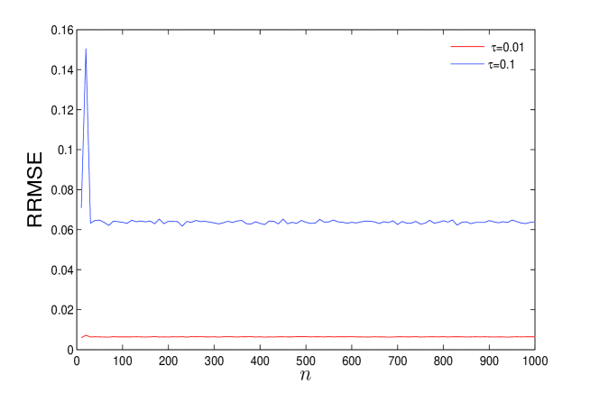
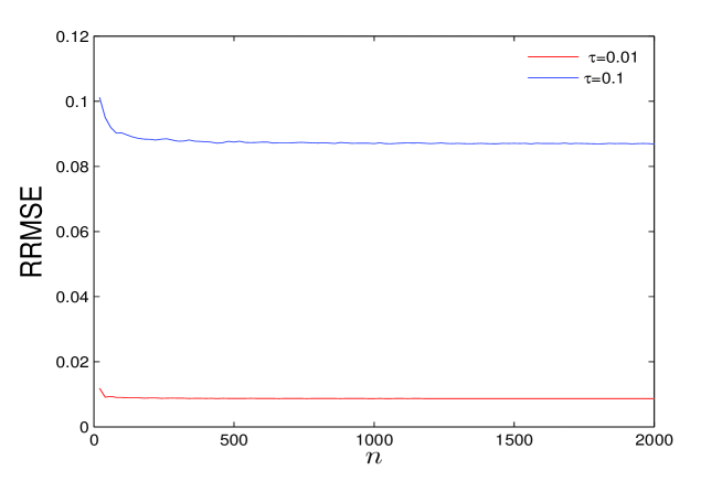
Next, we take $n,k,r\rightarrow\infty$ while the ratios $\frac{n}{k}=5$ and $\frac{k}{r}=4$ are kept constant, and compute the relative error for different noise level. Again, the relative error converges rapidly to constant, independent of $n,k,r$ .

Figure 6: Reconstruction error for $n\times n$ matrix $X$ with rank $r$ varying from $1$ to $50$ and with $n=20r,k=4r$. Two different noise level are shown: $\tau=0.1$ (blue) and $\tau=0.01$ (red). Each point represents average performance over $100$ random matrices.

7.6 Low Rank matrix Approximation

We bring here the one pass algorithm to approximate $X$ from [15] for the convenience of the reader. The output of this algorithm isn’t low rank if $k>r$. This algorithm is different from $SVLS_{P}$ and its purpose is to approximate a (possibly full rank) matrix by low rank matrix. We adjusted Algorithm 3 to our purpose with some changes. First, we estimate the rank of $X$ using the elbow method from Section 3.3 and instead of calculating the QR decomposition of $B^{(C)}$ and $B^{(R)^{T}}$ we find their $\hat{r}$ largest singular vectors. Furthermore, we repeat part two in algorithm 3 while replacing the roles of columns and rows as in SVLS . This variation gives our modified algorithm $SVLS_{P}$ as described in Section 3.4.

Input: $A^{(R)},A^{(C)},B^{(R)},B^{(C)}$

1. compute $Q^{(C)}R^{(C)}$ the QR decomposition of $B^{(C)}$, and $Q^{(R)}R^{(R)}$ the QR decomposition of $B^{(R)^{T}}$

2. Find the least-squares solution $Y=argmin_{C}||Q^{(C)}B^{(C)}-CQ^{(R)^{T}}B^{(R)^{T}}||_{F}$.

3. Return the estimate $\hat{X}=Q^{(C)}YQ^{(R)^{T}}$.

Algorithm 3

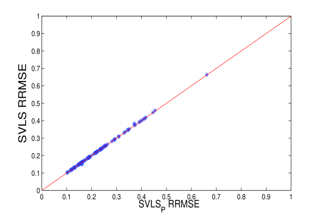
We compared our SVLS to $SVLS_{P}$ which is presented in Section 3.4. We took $X\in\mathcal{{M}}_{1000\times 1000}^{(10)}$ and $\sigma=1$. We tried to recover $X$ in the GRC model with $k=12$ for $100$ different matrices. For each matrix, we compared the $RRMSE$ obtained for the outputs of SVLS and $SVLS_{P}$. The $RRMSE$ for $SVLS_{P}$ was lower than the $RRMSE$ for SVLS in most cases but the differences were very small and negligible.

Figure 7: We recover a matrix $X$ from $24000$ measurements as in the GRC model $100$ times. Figure shows average $RRMSE$ over $100$ simulations for SVLS ($Y$ axis) and $SVLS_{P}$ ($X$ axis). The red linear line $Y=X$ was drawn for comparing those two algorithm, every dot that under the red line is a simulation that SVLS was better than $SVLS_{P}$ and every dot above the line tells the opposite

7.7 Rank Estimation

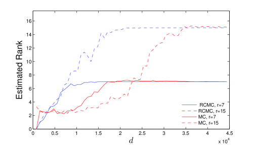
We test the elbow method for estimating the rank of $X$ (see eq. (10)). We take a matrix $X$ of size $400\times 400$ and different ranks. We add Gaussian noise with $\sigma=0.25$ while the measurements are sampled as in the RCMC model. For each number of measurements we sampled $100$ matrices and took the average estimated rank. We compute the estimator $\hat{r}$ for different values of $d$, the number of measurements. We compare our method to the rank estimation which appears in OptSpace [17] for the standard MC problem. Our simulation results, shown in Figure 8, indicate that the RCMC model with the elbow method is a much better design for rank estimation of $X$.

Figure 8: Estimation of $rank(X)$ vs. $d$, the number of measurements, $d=k(2n-k)$ where $k$ is the number of columns in $B^{(C)}$ and number of rows in $B^{(R)}$. For each $d$ we sampled $100$ different matrices. Estimation was performed by the elbow method for RCMC model, as in eq. (10) in the main text, and for the MC model we used the method described in [17]. RCMC recovers the correct rank with smaller number of measurements.

7.8 Test Error

In matrix completion with MC and RCMC ensembles the $RRMSE$ loss function measures the loss on both the observed and unobserved entries. This loss may be too optimistic when considering our prediction error only on unobserved entries. Thus, instead of including all measurements in calculation of the $RRMSE$ we compute a different measure of prediction error, given by the $RRMSE$ only on the unobserved entries. For each single-entry measurements operator $\mathcal{{A}}$ define $E(\mathcal{{A}})$ the set of measured entries and $\bar{E}$ it’s complement, i.e. the set of unmeasured entries $(i,j)\in[n_{1}]\times[n_{2}]$. We define $X^{\bar{E}}$ to be a matrix such that $X^{\bar{E}}_{ij}=X_{ij}$ if $(i,j)\in\bar{E}$ and $0$ otherwise. Instead of $RRMSE(X,\hat{X})$ we now calculate $RRMSE(X^{\bar{E}},\hat{X}^{\bar{E}})$. This quantity measures our reconstruction only on the unseen matrix entries $X_{ij}$, and is thus not influenced by overfitting. In Table 2 we performed exactly the same simulation as in Table 1 but with $RRMSE(X^{\bar{E}},\hat{X}^{\bar{E}})$. The results of OptSpace ​, SVT and SVLS stay similar to the results in Table 1 and our $RRMSE$ loss function does not show overfitting.

NR	$d$	$r$	SVLS	OptSpace	SVT
$10^{-2}\!\!\!$	$120156$	$10$	$0.006\quad(0.006)$	$0.004\quad(0.004)$	$0.0074\quad(0.0073)$
$10^{-1}\!\!\!$	$120156$	$10$	$0.065\quad(0.064)$	$0.045\quad(0.044)$	$0.051\quad(0.05)$
$1\!\!\!$	$120156$	$10$	$0.619\quad(0.612)$	$0.49\quad(0.49)$	$0.52\quad(0.51)$

Table 2: $RRMSE$ only on the unknown measurements. for SVLS applied to RCMC, and OptSpace and SVT applied to the standard MC. Results represent average of $5$ different random matrices. The results in the parentheses are the standard $RRMSE$ in Table 1.

References

- [1] Ronen Basri and David W Jacobs. Lambertian reflectance and linear subspaces. Pattern Analysis and Machine Intelligence, IEEE Transactions on, 25(2):218–233, 2003.
- [2] Jian-Feng Cai, Emmanuel J Candès, and Zuowei Shen. A singular value thresholding algorithm for matrix completion. SIAM Journal on Optimization, 20(4):1956–1982, 2010.
- [3] Tony T Cai and Anru Zhang. ROP: Matrix recovery via rank-one projections. The Annals of Statistics, 43(1):102–138, 2015.
- [4] Emmanuel J Candès and Yaniv Plan. Matrix completion with noise. Proceedings of the IEEE, 98(6):925–936, 2010.
- [5] Emmanuel J Candès and Yaniv Plan. Tight oracle inequalities for low-rank matrix recovery from a minimal number of noisy random measurements. IEEE Transactions on Information Theory, 57(4):2342–2359, 2011.
- [6] Emmanuel J Candès and Benjamin Recht. Exact matrix completion via convex optimization. Foundations of Computational Mathematics, 9(6):717–772, 2009.
- [7] Emmanuel J Candès and Justin Romberg. Sparsity and incoherence in compressive sampling. Inverse Problems, 23(3):969, 2007.
- [8] Emmanuel J Candès and Terence Tao. The power of convex relaxation: Near-optimal matrix completion. IEEE Transactions on Information Theory, 56(5):2053–2080, 2010.
- [9] Eric C Chi, Hua Zhou, Gary K Chen, Diego Ortega Del Vecchyo, and Kenneth Lange. Genotype imputation via matrix completion. Genome Research, 23(3):509–518, 2013.
- [10] Ci Chu, Kun Qu, Franklin L Zhong, Steven E Artandi, and Howard Y Chang. Genomic maps of long noncoding RNA occupancy reveal principles of RNA-chromatin interactions. Molecular cell, 44(4):667–678, 2011.
- [11] Sanjoy Dasgupta and Anupam Gupta. An elementary proof of a theorem of Johnson and Lindenstrauss. Random Structures & Algorithms, 22(1):60–65, 2003.
- [12] Carl Eckart and Gale Young. The approximation of one matrix by another of lower rank. Psychometrika, 1(3):211–218, 1936.
- [13] Matan Gavish and David L Donoho. The optimal hard threshold for singular values is . IEEE Transactions on Information Theory, 60(8):5040–5053, 2014.
- [14] David Gross, Yi-Kai Liu, Steven T Flammia, Stephen Becker, and Jens Eisert. Quantum state tomography via compressed sensing. Physical Review Letters, 105(15):150401, 2010.
- [15] Nathan Halko, Per-Gunnar Martinsson, and Joel A Tropp. Finding structure with randomness: Probabilistic algorithms for constructing approximate matrix decompositions. SIAM Review, 53(2):217–288, 2011.
- [16] Prateek Jain, Raghu Meka, and Inderjit S Dhillon. Guaranteed rank minimization via singular value projection. In Advances in Neural Information Processing Systems, pages 937–945, 2010.
- [17] Raghunandan H Keshavan, Andrea Montanari, and Sewoong Oh. Matrix completion from noisy entries. In Advances in Neural Information Processing Systems, pages 952–960, 2009.
- [18] Raghunandan H Keshavan, Andrea Montanari, and Sewoong Oh. Matrix completion from a few entries. IEEE Transactions on Information Theory, 56(6):2980–2998, 2010.
- [19] Yehuda Koren, Robert Bell, and Chris Volinsky. Matrix factorization techniques for recommender systems. Computer, 42(8):30–37, 2009.
- [20] Shiqian Ma, Donald Goldfarb, and Lifeng Chen. Fixed point and Bregman iterative methods for matrix rank minimization. Mathematical Programming, 128(1-2):321–353, 2011.
- [21] Benjamin Recht. A simpler approach to matrix completion. The Journal of Machine Learning Research, 12(Dec):3413–3430, 2011.
- [22] Benjamin Recht, Maryam Fazel, and Pablo A Parrilo. Guaranteed minimum-rank solutions of linear matrix equations via nuclear norm minimization. SIAM Review, 52(3):471–501, 2010.
- [23] Shai Shalev-Shwartz and Shai Ben-David. Understanding Machine Learning: From Theory to Algorithms. Cambridge University Press, 2014.
- [24] Stanislaw J Szarek. Condition numbers of random matrices. Journal of Complexity, 7(2):131–149, 1991.
- [25] Michel Talagrand. New concentration inequalities in product spaces. Inventiones Mathematicae, 126(3):505–563, 1996.
- [26] Kim-Chuan Toh and Sangwoon Yun. An accelerated proximal gradient algorithm for nuclear norm regularized linear least squares problems. Pacific Journal of Optimization, 6(3):615–640, 2010.