A Multilevel Correction Scheme for Nonsymmetric Eigenvalue Problems by Finite Element Methods

Hehu Xie LSEC, ICMSEC, NCMIS, Academy of Mathematics and Systems Science, Chinese Academy of Sciences, Beijing 100190, China (hhxie@lsec.cc.ac.cn).    Zhimin Zhang Beijing Computational Science Research Center, and Department of Mathematics, Wayne State University, Detroit, MI 48202, USA (zzhang@math.wayne.edu).
Abstract

A multilevel correction scheme is proposed to solve defective and nodefective of nonsymmetric partial differential operators by the finite element method. The method includes multi correction steps in a sequence of finite element spaces. In each correction step, we only need to solve two source problems on a finer finite element space and two eigenvalue problems on the coarsest finite element space. The accuracy of the eigenpair approximation is improved after each correction step. This correction scheme improves overall efficiency of the finite element method in solving nonsymmetric eigenvalue problems.

keywords:
Nonsymmetric eigenvalue problem, multilevel correction, finite element method, high-efficiency
AMS:
65N30, 65N25, 65L15, 65B99

1 Introduction

As we know, the numerical approximation of eigenvalue problems plays a central role in the analysis of the stability for nonlinear partial differential equations. For example in fluid mechanics, the analysis of the hydrodynamic stability always leads to a nonsymmetric eigenvalue problems (see [1, 7, 8]). The stability of the underlying flow depends on the real part of the eigenvalue which has the smallest real part (see [1, 8]). For more details, please refer [1, 8, 15]. The aim of understanding the stability of nonlinear partial differential equations naturally leads to the computation of the eigenvalue problems with some numerical methods. The main content of this paper is to design an efficient finite element method to compute nonsymmetric eigenvalue problems.

Recently, a multigrid method is designed to solve the self-adjoint eigenvalue problem based on a type of multilevel correction method [10, 11, 12, 18]. But as we know, the analysis of the stability for nonlinear partial differential equations always leads to nonsymmetric eigenvalue problems [1, 8] and the extensions of the multilevel method for self-adjoint eigenvalue problems to the nonsymmetric ones is not direct [9, 23, 25] and needs more analysis. So the purpose of this paper is to propose a multilevel correction scheme to solve nonsymmetric eigenvalue problems based on the finite element method. In the past, a two-grid finite element method was proposed and analyzed by Xu and Zhou in [23] for symmetric eigenvalue problems. Latter, Kolman used this idea to design a two-level method for nonsymmetric eigenvalue problems in [9]. Yang and Fan [25] also studied a two-grid method for nonsymmetric eigenvalue problems. As an alternative approach, in [13, 14, 17], the authors used a recovery technique PPR to improve the convergence rate for both symmetric and nonsymmetric eigenvalue problems. All these methods are designed for the nonsymmetric eigenvalue problems under the assumption that the ascent of the concerned eigenvalues is only one which means the algebraic eigenspace is the same as the geometric eigenspace.

Along the line of multilevel correction method, here we present a multilevel correction scheme to solve nonsymmetric eigenvalue problems without the ascent assumption. With the proposed method, solving nonsymmetric eigenvalue problems will not be much more expensive than solving corresponding source problems. The correction method for eigenvalue problems in this paper is based on a series of finite element spaces with different levels of accuracy which are related to the multilevel method (cf. [20]).

The standard Galerkin finite element method for nonsymmetric eigenvalue problems has been extensively investigated, e.g. Babuška and Osborn [2, 3], Chatelin [5] and references cited therein. Here we adopt some basic results in these papers to carry on error estimates for our multilevel correction scheme. It will be shown that the convergence rate of the eigenpair approximations can be improved after each correction step.

Our multilevel correction procedure can be described as follows: (1) solve an eigenvalue problem in the coarsest finite element space; (2) solve a source problem in an augmented space with the associated eigenfunction from (1) as the load vector; (3) solve the eigenvalue problem again on a finite element space constructed by enhancing the coarsest finite element space with the eigenfunction obtained in step (2). Then go to step (2) for the next loop.

In this method, we replace solving the eigenvalue problem in finer finite element spaces by solving a series of boundary value problems in a series of nested finite element spaces (with the finest space as the last one) and a series of eigenvalue problems in the coarsest finite element space; and yet, we achieve the same accuracy as solving the eigenvalue problem in the finest space. It is well known that there exist multigrid methods that solve boundary value problems with the optimal computational work (cf. [21]). Therefore, combined with the multigrid method, our correction method improves overall efficiency in solving nonsymmetric eigenvalue problems (cf. [18, 19]).

An outline of the paper goes as follows. In Section 2, we introduce the finite element method for nonsymmetric eigenvalue problems. An one level correction scheme is described and analyzed in Section 3. In Section 4, we propose and analyze a multilevel correction algorithm to solve nonsymmetric eigenvalue problems by the finite element method. Some numerical examples are presented in Section 5 to validate our theoretical analysis and some concluding remarks are given in the last section.

2 Discretization by finite element method

In this section, we introduce some notation and error estimates of the finite element approximation for nonsymmetric eigenvalue problems. Throughout this paper, the letter C𝐶C (with or without subscripts) denotes a generic positive constant which may be different at different occurrences. For convenience, we use symbols less-than-or-similar-to\lesssim, greater-than-or-equivalent-to\gtrsim, and \approx, such that x1y1,x2y2formulae-sequenceless-than-or-similar-tosubscript𝑥1subscript𝑦1greater-than-or-equivalent-tosubscript𝑥2subscript𝑦2x_{1}\lesssim y_{1},x_{2}\gtrsim y_{2}, and x3y3subscript𝑥3subscript𝑦3x_{3}\approx y_{3} have meanings: x1C1y1subscript𝑥1subscript𝐶1subscript𝑦1x_{1}\leq C_{1}y_{1}, x2c2y2subscript𝑥2subscript𝑐2subscript𝑦2x_{2}\geq c_{2}y_{2}, and c3x3y3C3x3subscript𝑐3subscript𝑥3subscript𝑦3subscript𝐶3subscript𝑥3c_{3}x_{3}\leq y_{3}\leq C_{3}x_{3}, for some constants C1,c2,c3subscript𝐶1subscript𝑐2subscript𝑐3C_{1},c_{2},c_{3}, and C3subscript𝐶3C_{3} that are independent of mesh sizes (cf. [20]).

We consider the following eigenvalue problem:

Find λ𝒞𝜆𝒞\lambda\in\mathcal{C} and u𝑢u such that

{(Au)+𝐛u+ϕu=λφu,inΩ,u=0,onΩ,Ωφ|u|2𝑑Ω=1,cases𝐴𝑢𝐛𝑢italic-ϕ𝑢𝜆𝜑𝑢inΩ𝑢0onΩsubscriptΩ𝜑superscript𝑢2differential-dΩ1\left\{\begin{array}[]{rcl}-\nabla\cdot(A\nabla u)+\mathbf{b}\cdot\nabla u+\phi u&=&\lambda\varphi u,\ \ \ {\rm in}\ \Omega,\\ u&=&0,\ \ \ \ \ \ \ {\rm on}\ \partial\Omega,\\ \int_{\Omega}\varphi|u|^{2}d\Omega&=&1,\end{array}\right. (1)

where ΩdΩsuperscript𝑑\Omega\subset\mathcal{R}^{d} is a bounded polygonal domain, A𝒞d×d𝐴superscript𝒞𝑑𝑑A\in\mathcal{C}^{d\times d}, 𝐛𝒞d𝐛superscript𝒞𝑑\mathbf{b}\in\mathcal{C}^{d}, ϕitalic-ϕ\phi is a function defined on ΩΩ\Omega and φ𝜑\varphi is a real positive function with φc0>0𝜑subscript𝑐00\varphi\geq c_{0}>0.

We define V:=H01(Ω)assign𝑉superscriptsubscript𝐻01ΩV:=H_{0}^{1}(\Omega) with the usual norm 1\|\cdot\|_{1}. The corresponding variational form of (1) can be stated as follows:

Find (λ,u)𝒞×V𝜆𝑢𝒞𝑉(\lambda,u)\in\mathcal{C}\times V such that b(u,u)=1𝑏𝑢𝑢1b(u,u)=1 and

a(u,v)𝑎𝑢𝑣\displaystyle a(u,v) =\displaystyle= λb(u,v),vV,𝜆𝑏𝑢𝑣for-all𝑣𝑉\displaystyle\lambda b(u,v),\ \ \ \ \ \forall v\in V, (2)

where

a(u,v)𝑎𝑢𝑣\displaystyle a(u,v) =\displaystyle= (Au,v¯)+(𝐛u,v¯)+(ϕu,v¯),𝐴𝑢¯𝑣𝐛𝑢¯𝑣italic-ϕ𝑢¯𝑣\displaystyle(A\nabla u,\overline{\nabla v})+(\mathbf{b}\cdot\nabla u,\bar{v})+(\phi u,\bar{v}),
b(u,v)𝑏𝑢𝑣\displaystyle b(u,v) =\displaystyle= (φu,v¯)𝜑𝑢¯𝑣\displaystyle(\varphi u,\bar{v})

with (,)(\cdot,\cdot) denoting the inner product in the space L2(Ω)superscript𝐿2ΩL^{2}(\Omega). The corresponding adjoint eigenvalue problem is:

Find (λ,u)𝒞×V𝜆superscript𝑢𝒞𝑉(\lambda,u^{*})\in\mathcal{C}\times V such that b(u,u)=1𝑏superscript𝑢superscript𝑢1b(u^{*},u^{*})=1 and

a(v,u)𝑎𝑣superscript𝑢\displaystyle a(v,u^{*}) =\displaystyle= λb(v,u),vV.𝜆𝑏𝑣superscript𝑢for-all𝑣𝑉\displaystyle\lambda b(v,u^{*}),\ \ \ \ \ \forall v\in V. (3)

In the sequel, we also use the norm vb=b(v,v)subscriptnorm𝑣𝑏𝑏𝑣𝑣\|v\|_{b}=\sqrt{b(v,v)} which is equivalent to the L2(Ω)superscript𝐿2ΩL^{2}(\Omega) norm 0\|\cdot\|_{0}. Here the bilinear form a(,)𝑎a(\cdot,\cdot) is assumed to satisfy

w1supvVa(w,v)v1andw1supvVa(v,w)v1,wV.formulae-sequenceless-than-or-similar-tosubscriptnorm𝑤1subscriptsupremum𝑣𝑉𝑎𝑤𝑣subscriptnorm𝑣1andformulae-sequenceless-than-or-similar-tosubscriptnorm𝑤1subscriptsupremum𝑣𝑉𝑎𝑣𝑤subscriptnorm𝑣1for-all𝑤𝑉\displaystyle\|w\|_{1}\lesssim\sup_{{v}\in V}\frac{a(w,v)}{\|v\|_{1}}\ \ {\rm and}\ \ \|w\|_{1}\lesssim\sup_{v\in V}\frac{a(v,w)}{\|v\|_{1}},\ \ \forall w\in V. (4)

We further assume that a(,)𝑎a(\cdot,\cdot) is V𝑉V-elliptic, i.e.,

u12superscriptsubscriptnorm𝑢12\displaystyle\|u\|_{1}^{2} less-than-or-similar-to\displaystyle\lesssim Rea(u,u),uV.Re𝑎𝑢𝑢for-all𝑢𝑉\displaystyle{\rm Re}\ a(u,u),\ \ \ \ \forall u\in V. (5)

2.1 Operator reformulation

We introduce the operators T,T(V)𝑇subscript𝑇𝑉T,\ T_{*}\in\mathcal{L}(V) defined by the equation

a(Tu,v)=b(u,v)=a(u,Tv),u,vV.formulae-sequence𝑎𝑇𝑢𝑣𝑏𝑢𝑣𝑎𝑢subscript𝑇𝑣for-all𝑢𝑣𝑉\displaystyle a(Tu,v)=b(u,v)={a}(u,T_{*}v),\ \ \ \ \ \forall u,v\in V. (6)

The eigenvalue problem (2) can be written as an operator form for λ0𝜆0\lambda\neq 0 (denoting μ:=λ1assign𝜇superscript𝜆1\mu:=\lambda^{-1}):

Tu=μu,𝑇𝑢𝜇𝑢\displaystyle Tu=\mu u, (7)

with

Tu=μ¯usubscript𝑇superscript𝑢¯𝜇superscript𝑢\displaystyle T_{*}u^{*}=\bar{\mu}u^{*} (8)

for the adjoint eigenvalue problem (3). Note that ellipticity condition (5) guarantees that every eigenvalue λ𝜆\lambda is nonzero. It is well known that the operators T𝑇T and Tsubscript𝑇T_{*} are compact. Thus the spectral theory for compact operators gives us a complete characterization of the eigenvalue problem (2).

There is a countable set of eigenvalues of (2). Let λ𝜆\lambda be an eigenvalue of problem (2). There exists a smallest integer α𝛼\alpha which are called the ascent such that

N((Tμ)α)=N((Tμ)α+1),𝑁superscript𝑇𝜇𝛼𝑁superscript𝑇𝜇𝛼1\displaystyle N((T-\mu)^{\alpha})=N((T-\mu)^{\alpha+1}), (9)

where N𝑁N denotes the null space and we use the notation μ=λ1𝜇superscript𝜆1\mu=\lambda^{-1}. Let M(λ)=Mλ,μ=N((Tμ)α)𝑀𝜆subscript𝑀𝜆𝜇𝑁superscript𝑇𝜇𝛼M(\lambda)=M_{\lambda,\mu}=N((T-\mu)^{\alpha}) and Q(λ)=Qλ,μ=N(Tμ)𝑄𝜆subscript𝑄𝜆𝜇𝑁𝑇𝜇Q(\lambda)=Q_{\lambda,\mu}=N(T-\mu) denote the algebraic and geometric eigenspaces, respectively. The subspaces Q(λ)M(λ)𝑄𝜆𝑀𝜆Q(\lambda)\subset M(\lambda) are finite dimensional. The numbers m=dimM(λ)𝑚dim𝑀𝜆m={\rm dim}M(\lambda) and q=dimQ(λ)𝑞dim𝑄𝜆q={\rm dim}Q(\lambda) are called the algebraic and the geometric multiplicities of μ𝜇\mu (and λ𝜆\lambda). The vectors in M(λ)𝑀𝜆M(\lambda) are generalized eigenvectors. The order of a generalized eigenvector is the smallest integer j𝑗j such that (Tμ)ju=0superscript𝑇𝜇𝑗𝑢0(T-\mu)^{j}u=0 (vectors in Q(λ)𝑄𝜆Q(\lambda) being generalized eigenvectors of order 111). Let us point out that a generalized eigenvector ujsuperscript𝑢𝑗u^{j} of order j𝑗j satisfies

a(uj,v)𝑎superscript𝑢𝑗𝑣\displaystyle a(u^{j},v) =\displaystyle= λb(uj,v)+λa(uj1,v),vV,𝜆𝑏superscript𝑢𝑗𝑣𝜆𝑎superscript𝑢𝑗1𝑣for-all𝑣𝑉\displaystyle\lambda b(u^{j},v)+\lambda a(u^{j-1},v),\ \ \ \ \forall v\in V, (10)

where uj1superscript𝑢𝑗1u^{j-1} is a generalized eigenvector of order j1𝑗1j-1.

Similarly we define the spaces of (generalized) eigenvectors for the adjoint problem

M(λ)=Mλ,μ=N((Tμ¯)α)andQ(λ)=Qλ,μ=N(Tμ¯).formulae-sequencesuperscript𝑀𝜆superscriptsubscript𝑀𝜆𝜇𝑁superscriptsubscript𝑇¯𝜇𝛼andsuperscript𝑄𝜆subscriptsuperscript𝑄𝜆𝜇𝑁subscript𝑇¯𝜇\displaystyle M^{*}(\lambda)=M_{\lambda,\mu}^{*}=N((T_{*}-\bar{\mu})^{\alpha})\ \ \ {\rm and}\ \ \ Q^{*}(\lambda)=Q^{*}_{\lambda,\mu}=N(T_{*}-\bar{\mu}).

Note that μ𝜇\mu is an eigenvalue of T𝑇T (λ𝜆\lambda is an eigenvalue of problem (2)) if and only if μ¯¯𝜇\bar{\mu} is an eigenvalue of Tsubscript𝑇T_{*} (λ𝜆\lambda is an eigenvalue of adjoint problem (3)) with the ascent α𝛼\alpha and the algebraic multiplicity m𝑚m for both eigenvalues being the same.

2.2 Galerkin discretization

Now, let us define the finite element approximations for the problem (2). First we generate a shape-regular decomposition of the computing domain Ωd(d=2,3)Ωsuperscript𝑑𝑑23\Omega\subset\mathcal{R}^{d}\ (d=2,3) into triangles or rectangles for d=2𝑑2d=2 (tetrahedrons or hexahedrons for d=3𝑑3d=3). The diameter of a cell K𝒯h𝐾subscript𝒯K\in\mathcal{T}_{h} is denoted by hKsubscript𝐾h_{K}. The mesh diameter hh describes the maximum diameter of all cells K𝒯h𝐾subscript𝒯K\in\mathcal{T}_{h}. Based on the mesh 𝒯hsubscript𝒯\mathcal{T}_{h}, we construct a finite element space denoted by VhVsubscript𝑉𝑉V_{h}\subset V. In order to define our multilevel correction method, we start the process on an initial mesh 𝒯Hsubscript𝒯𝐻\mathcal{T}_{H} with mesh size H𝐻H and the initial finite element space VHsubscript𝑉𝐻V_{H} defined on 𝒯Hsubscript𝒯𝐻\mathcal{T}_{H}. In this paper, the finite element space Vhsubscript𝑉V_{h} is assumed to satisfy

wh1supvhVha(wh,vh)vh1andwh1supvhVha(vh,wh)vh1,whVh.formulae-sequenceless-than-or-similar-tosubscriptnormsubscript𝑤1subscriptsupremumsubscript𝑣subscript𝑉𝑎subscript𝑤subscript𝑣subscriptnormsubscript𝑣1andformulae-sequenceless-than-or-similar-tosubscriptnormsubscript𝑤1subscriptsupremumsubscript𝑣subscript𝑉𝑎subscript𝑣subscript𝑤subscriptnormsubscript𝑣1for-allsubscript𝑤subscript𝑉\displaystyle\|w_{h}\|_{1}\lesssim\sup_{v_{h}\in V_{h}}\frac{a(w_{h},v_{h})}{\|v_{h}\|_{1}}\ \ {\rm and}\ \ \|w_{h}\|_{1}\lesssim\sup_{v_{h}\in V_{h}}\frac{a(v_{h},w_{h})}{\|v_{h}\|_{1}},\ \ \forall w_{h}\in V_{h}. (11)

The standard Galerkin discretization of the problem (2) is the following:

Find (λh,uh)𝒞×Vhsubscript𝜆subscript𝑢𝒞subscript𝑉(\lambda_{h},u_{h})\in\mathcal{C}\times V_{h} such that b(uh,uh)=1𝑏subscript𝑢subscript𝑢1b(u_{h},u_{h})=1 and

a(uh,vh)𝑎subscript𝑢subscript𝑣\displaystyle a(u_{h},v_{h}) =\displaystyle= λhb(uh,vh),vhVh.subscript𝜆𝑏subscript𝑢subscript𝑣for-allsubscript𝑣subscript𝑉\displaystyle\lambda_{h}b(u_{h},v_{h}),\ \ \ \ \ \forall v_{h}\in V_{h}. (12)

Similarly, the discretization of the adjoint problem (3) can be defined as:

Find (λh,uh)𝒞×Vhsubscript𝜆superscriptsubscript𝑢𝒞subscript𝑉(\lambda_{h},u_{h}^{*})\in\mathcal{C}\times V_{h} such that b(uh,uh)=1𝑏superscriptsubscript𝑢superscriptsubscript𝑢1b(u_{h}^{*},u_{h}^{*})=1 and

a(vh,uh)𝑎subscript𝑣superscriptsubscript𝑢\displaystyle a(v_{h},{u_{h}^{*}}) =\displaystyle= λhb(vh,uh),vhVh.subscript𝜆𝑏subscript𝑣superscriptsubscript𝑢for-allsubscript𝑣subscript𝑉\displaystyle\lambda_{h}b(v_{h},{u_{h}^{*}}),\ \ \ \ \ \forall v_{h}\in V_{h}. (13)

By introducing Galerkin projections Ph,Ph(V,Vh)subscript𝑃superscriptsubscript𝑃𝑉subscript𝑉P_{h},\ P_{h}^{*}\in\mathcal{L}(V,V_{h}) with the following equations

a(Phu,vh)𝑎subscript𝑃𝑢subscript𝑣\displaystyle a(P_{h}u,v_{h}) =\displaystyle= a(u,vh),uV,vhVh,formulae-sequence𝑎𝑢subscript𝑣for-all𝑢𝑉for-allsubscript𝑣subscript𝑉\displaystyle a(u,v_{h}),\ \ \ \ \ \quad\forall u\in V,\ \forall v_{h}\in V_{h},
a(vh,u)𝑎subscript𝑣𝑢\displaystyle a(v_{h},u) =\displaystyle= a(vh,Phu),uV,vhVh,formulae-sequence𝑎subscript𝑣superscriptsubscript𝑃𝑢for-all𝑢𝑉for-allsubscript𝑣subscript𝑉\displaystyle a(v_{h},P_{h}^{*}u),\ \ \ \ \forall u\in V,\ \forall v_{h}\in V_{h},

the equation (12) can be rewritten as an operator form with μh:=λh1assignsubscript𝜇superscriptsubscript𝜆1\mu_{h}:=\lambda_{h}^{-1} (Note that Phsubscript𝑃P_{h} is a bounded operator),

PhTuh=μhuh.subscript𝑃𝑇subscript𝑢subscript𝜇subscript𝑢\displaystyle P_{h}Tu_{h}=\mu_{h}u_{h}. (14)

Similarly for the adjoint problem (13), we have

PhTuh=μ¯huh.superscriptsubscript𝑃subscript𝑇superscriptsubscript𝑢subscript¯𝜇superscriptsubscript𝑢\displaystyle P_{h}^{*}T_{*}u_{h}^{*}=\bar{\mu}_{h}u_{h}^{*}. (15)

2.3 Spectral approximation of compact operators

Let μ𝜇\mu be an eigenvalue (with algebraic multiplicity m𝑚m) of the compact operator T𝑇T. If T𝑇T is approximated by a sequence of compact operators Thsubscript𝑇T_{h} converging to T𝑇T in norm, i.e., limh0+TTh1=0subscriptlimit-from0subscriptnorm𝑇subscript𝑇10\lim\limits_{h\rightarrow 0+}{\|T-T_{h}\|_{1}}=0, then for hh sufficiently small μ𝜇\mu is approximated by m𝑚m numerical eigenvalues {μj,h}j=1,,msubscriptsubscript𝜇𝑗𝑗1𝑚\{\mu_{j,h}\}_{j=1,\cdots,m} (counted according to their algebraic multiplicities) of Thsubscript𝑇T_{h}, i.e.,

limh0+μj,h=μforj=1,,m.formulae-sequencesubscriptlimit-from0subscript𝜇𝑗𝜇for𝑗1𝑚\displaystyle\lim_{h\rightarrow 0+}\mu_{j,h}=\mu\ \ \ \ \ {\rm for}\ j=1,\cdots,m.

The space of generalized eigenvectors of T𝑇T is approximated by the subspace

Mh(λ)=Mhλ,μ=j=1mN((Thμj,h)αμj,h),subscript𝑀𝜆superscriptsubscript𝑀𝜆𝜇superscriptsubscript𝑗1𝑚𝑁superscriptsubscript𝑇subscript𝜇𝑗subscript𝛼subscript𝜇𝑗\displaystyle M_{h}(\lambda)=M_{h}^{\lambda,\mu}=\sum_{j=1}^{m}N((T_{h}-\mu_{j,h})^{\alpha_{\mu_{j,h}}}), (16)

where αμj,hsubscript𝛼subscript𝜇𝑗\alpha_{\mu_{j,h}} is the smallest integer such that N((Thμj,h)αμj,h)=N((Thμj,h)αμj,h+1)𝑁superscriptsubscript𝑇subscript𝜇𝑗subscript𝛼subscript𝜇𝑗𝑁superscriptsubscript𝑇subscript𝜇𝑗subscript𝛼subscript𝜇𝑗1N((T_{h}-\mu_{j,h})^{\alpha_{\mu_{j,h}}})=N((T_{h}-\mu_{j,h})^{\alpha_{\mu_{j,h}}+1}). We similarly define the space Qh(λ)=Qhλ,μ=j=1mN(Thμj,h)subscript𝑄𝜆superscriptsubscript𝑄𝜆𝜇superscriptsubscript𝑗1𝑚𝑁subscript𝑇subscript𝜇𝑗Q_{h}(\lambda)=Q_{h}^{\lambda,\mu}=\sum_{j=1}^{m}N(T_{h}-\mu_{j,h}) and counterparts Mh(λ)superscriptsubscript𝑀𝜆M_{h}^{*}(\lambda), Qh(λ)superscriptsubscript𝑄𝜆Q_{h}^{*}(\lambda) for the adjoint problem .

Now, we describe a computational scheme to produce the algebraic eigenspace Mh(λ)subscript𝑀𝜆M_{h}(\lambda) from the geometric eigenspace Qh(λ)={u1,h,,uq,h}subscript𝑄𝜆subscript𝑢1subscript𝑢𝑞Q_{h}(\lambda)=\{u_{1,h},\cdots,u_{q,h}\} corresponding to eigenvalues {λ1,h,,λq,h}subscript𝜆1subscript𝜆𝑞\{\lambda_{1,h},\cdots,\lambda_{q,h}\}, which converge to the same eigenvalue λ𝜆\lambda.

Starting from all eigenfunctions in the geometric eigenspace Qh(λ)subscript𝑄𝜆Q_{h}(\lambda) (of order 111), we use the following recursive process to compute algebraic eigenspaces (cf. [16])

{a(uj,h,vh)λj,hb(uj,h,vh)=λj,ha(uj,h1,vh),vhVh,b(uj,h,vh)=0,vhQh(λ),cases𝑎superscriptsubscript𝑢𝑗subscript𝑣subscript𝜆𝑗𝑏superscriptsubscript𝑢𝑗subscript𝑣subscript𝜆𝑗𝑎superscriptsubscript𝑢𝑗1subscript𝑣for-allsubscript𝑣subscript𝑉𝑏superscriptsubscript𝑢𝑗subscript𝑣0for-allsubscript𝑣subscript𝑄𝜆\left\{\begin{array}[]{rcl}a(u_{j,h}^{\ell},v_{h})-\lambda_{j,h}b(u_{j,h}^{\ell},v_{h})&=&\lambda_{j,h}a(u_{j,h}^{\ell-1},v_{h}),\ \ \forall v_{h}\in V_{h},\\ b(u_{j,h}^{\ell},v_{h})&=&0,\ \ \ \quad\quad\quad\quad\quad\ \ \forall v_{h}\in Q_{h}({\lambda}),\end{array}\right. (17)

where 22\ell\geq 2, uj,hsuperscriptsubscript𝑢𝑗u_{j,h}^{\ell} is the general eigenfunction of order \ell and uj,h1=uj,hQh(λ)superscriptsubscript𝑢𝑗1subscript𝑢𝑗subscript𝑄𝜆u_{j,h}^{1}=u_{j,h}\in Q_{h}({\lambda}) for j=1,,q𝑗1𝑞j=1,\cdots,q.

With the above process, we generate the algebraic eigenspace

Mh(λ)={u1,h,,uq,h,,um,h}subscript𝑀𝜆subscript𝑢1subscript𝑢𝑞subscript𝑢𝑚M_{h}(\lambda)=\{u_{1,h},\cdots,u_{q,h},\cdots,u_{m,h}\}

corresponding to eigenvalues {λ1,h,,λq,h,,λm,h}subscript𝜆1subscript𝜆𝑞subscript𝜆𝑚\{\lambda_{1,h},\cdots,\lambda_{q,h},\cdots,\lambda_{m,h}\}, which converge to the same eigenvalue λ𝜆\lambda. Similarly, we can produce the adjoint algebraic eigenspace Mh(λ)superscriptsubscript𝑀𝜆M_{h}^{*}(\lambda) from the geometric eigenspace Qh(λ)superscriptsubscript𝑄𝜆Q_{h}^{*}(\lambda).

For two linear spaces A𝐴A and B𝐵B, we denote

Θ^(A,B)=supwA,w1=1infvBwv1,Φ^(A,B)=supwA,wb=1infvBwvb,formulae-sequence^Θ𝐴𝐵subscriptsupremumformulae-sequence𝑤𝐴subscriptnorm𝑤11subscriptinfimum𝑣𝐵subscriptnorm𝑤𝑣1^Φ𝐴𝐵subscriptsupremumformulae-sequence𝑤𝐴subscriptnorm𝑤𝑏1subscriptinfimum𝑣𝐵subscriptnorm𝑤𝑣𝑏\displaystyle\widehat{\Theta}(A,B)=\sup_{w\in A,\|w\|_{1}=1}\inf_{v\in B}\|w-v\|_{1},\ \ \widehat{\Phi}(A,B)=\sup_{w\in A,\|w\|_{b}=1}\inf_{v\in B}\|w-v\|_{b},

and define gaps between A𝐴A and B𝐵B in 1\|\cdot\|_{1} as

Θ(A,B)=max{Θ^(A,B),Θ^(B,A)},Θ𝐴𝐵^Θ𝐴𝐵^Θ𝐵𝐴\displaystyle\Theta(A,B)=\max\big{\{}\widehat{\Theta}(A,B),\widehat{\Theta}(B,A)\big{\}}, (18)

and in b\|\cdot\|_{b} as

Φ(A,B)=max{Φ^(A,B),Φ^(B,A)}.Φ𝐴𝐵^Φ𝐴𝐵^Φ𝐵𝐴\displaystyle\Phi(A,B)=\max\big{\{}\widehat{\Phi}(A,B),\widehat{\Phi}(B,A)\big{\}}. (19)

Before introducing the convergence results of the finite element approximation for nonsymmetric eigenvalue problems, we define the following notation

δh(λ)=supuM(λ),u1=1infvhVhuvh1,subscript𝛿𝜆subscriptsupremumformulae-sequence𝑢𝑀𝜆subscriptnorm𝑢11subscriptinfimumsubscript𝑣subscript𝑉subscriptnorm𝑢subscript𝑣1\displaystyle\delta_{h}(\lambda)=\sup_{{u}\in M(\lambda),\|u\|_{1}=1}\inf_{v_{h}\in V_{h}}\|u-v_{h}\|_{1}, (20)
δh(λ)=supuM(λ),u1=1infvhVhuvh1,superscriptsubscript𝛿𝜆subscriptsupremumformulae-sequencesuperscript𝑢superscript𝑀𝜆subscriptnormsuperscript𝑢11subscriptinfimumsubscript𝑣subscript𝑉subscriptnormsuperscript𝑢subscript𝑣1\displaystyle\delta_{h}^{*}(\lambda)=\sup_{u^{*}\in M^{*}(\lambda),\|u^{*}\|_{1}=1}\inf_{v_{h}\in V_{h}}\|u^{*}-v_{h}\|_{1}, (21)
ρh(λ)=supuM(λ),ub=1infvhVhuvhb,subscript𝜌𝜆subscriptsupremumformulae-sequence𝑢𝑀𝜆subscriptnorm𝑢𝑏1subscriptinfimumsubscript𝑣subscript𝑉subscriptnorm𝑢subscript𝑣𝑏\displaystyle\rho_{h}(\lambda)=\sup_{{u}\in M(\lambda),\|u\|_{b}=1}\inf_{v_{h}\in V_{h}}\|u-v_{h}\|_{b}, (22)
ρh(λ)=supuM(λ),ub=1infvhVhuvhb,superscriptsubscript𝜌𝜆subscriptsupremumformulae-sequencesuperscript𝑢superscript𝑀𝜆subscriptnormsuperscript𝑢𝑏1subscriptinfimumsubscript𝑣subscript𝑉subscriptnormsuperscript𝑢subscript𝑣𝑏\displaystyle\rho_{h}^{*}(\lambda)=\sup_{u^{*}\in M^{*}(\lambda),\|u^{*}\|_{b}=1}\inf_{v_{h}\in V_{h}}\|u^{*}-v_{h}\|_{b}, (23)
ηa(h)=supfV,fb=1infvVhTfv1,subscript𝜂𝑎subscriptsupremumformulae-sequence𝑓𝑉subscriptnorm𝑓𝑏1subscriptinfimum𝑣subscript𝑉subscriptnorm𝑇𝑓𝑣1\displaystyle\eta_{a}(h)=\sup_{f\in V,\|f\|_{b}=1}\inf_{v\in V_{h}}\|Tf-v\|_{1}, (24)
ηa(h)=supfV,fb=1infvVhTfv1.superscriptsubscript𝜂𝑎subscriptsupremumformulae-sequence𝑓𝑉subscriptnorm𝑓𝑏1subscriptinfimum𝑣subscript𝑉subscriptnormsubscript𝑇𝑓𝑣1\displaystyle\eta_{a}^{*}(h)=\sup_{f\in V,\|f\|_{b}=1}\inf_{v\in V_{h}}\|T_{*}f-v\|_{1}. (25)

In order to derive error bounds for eigenpair approximations in the weak norm b\|\cdot\|_{b}, we need the following error estimates in the weak norm b\|\cdot\|_{b} of the finite element approximation.

Lemma 1.

([3, Lemma 3.3 and Lemma 3.4])

ηa(h)=o(1),ηa(h)=o(1)ash0,formulae-sequencesubscript𝜂𝑎𝑜1formulae-sequencesuperscriptsubscript𝜂𝑎𝑜1as0\displaystyle\eta_{a}(h)=o(1),\ \ \ \eta_{a}^{*}(h)=o(1)\ \ \ {\rm as}\ h\rightarrow 0, (26)

and

ρh(λ)subscript𝜌𝜆\displaystyle\rho_{h}(\lambda) less-than-or-similar-to\displaystyle\lesssim ηa(h)δh(λ),superscriptsubscript𝜂𝑎subscript𝛿𝜆\displaystyle\eta_{a}^{*}(h)\delta_{h}(\lambda), (27)
ρh(λ)superscriptsubscript𝜌𝜆\displaystyle\rho_{h}^{*}(\lambda) less-than-or-similar-to\displaystyle\lesssim ηa(h)δh(λ).subscript𝜂𝑎superscriptsubscript𝛿𝜆\displaystyle\eta_{a}(h)\delta_{h}^{*}(\lambda). (28)

The following theorem is a basic tool for our error estimates.

Theorem 2.

([3, Section 8]) When the mesh size hh is small enough, we have

Θ(M(λ),Mh(λ))δh(λ),Θ(M(λ),Mh(λ))δh(λ),formulae-sequenceless-than-or-similar-toΘ𝑀𝜆subscript𝑀𝜆subscript𝛿𝜆less-than-or-similar-toΘsuperscript𝑀𝜆subscriptsuperscript𝑀𝜆subscriptsuperscript𝛿𝜆\displaystyle\Theta(M(\lambda),M_{h}(\lambda))\lesssim\delta_{h}(\lambda),\ \ \ \Theta(M^{*}(\lambda),M^{*}_{h}(\lambda))\lesssim\delta^{*}_{h}(\lambda), (29)
Φ(M(λ),Mh(λ))ρh(λ),Φ(M(λ),Mh(λ))ρh(λ),formulae-sequenceless-than-or-similar-toΦ𝑀𝜆subscript𝑀𝜆subscript𝜌𝜆less-than-or-similar-toΦsuperscript𝑀𝜆subscriptsuperscript𝑀𝜆subscriptsuperscript𝜌𝜆\displaystyle\Phi(M(\lambda),M_{h}(\lambda))\lesssim\rho_{h}(\lambda),\ \ \ \Phi(M^{*}(\lambda),M^{*}_{h}(\lambda))\lesssim\rho^{*}_{h}(\lambda), (30)
|λλ^h|δh(λ)δh(λ),less-than-or-similar-to𝜆subscript^𝜆subscript𝛿𝜆superscriptsubscript𝛿𝜆\displaystyle|\lambda-\widehat{\lambda}_{h}|\lesssim\delta_{h}(\lambda)\delta_{h}^{*}(\lambda), (31)

where λ^h=1mj=1mλj,hsubscript^𝜆1𝑚superscriptsubscript𝑗1𝑚subscript𝜆𝑗\widehat{\lambda}_{h}={\frac{1}{m}}\sum_{j=1}^{m}\lambda_{j,h} with λ1,h,,λm,hsubscript𝜆1subscript𝜆𝑚\lambda_{1,h},\cdots,\lambda_{m,h} converging to λ𝜆\lambda.

3 One correction step

In this section, we present an one-step correction procedure to improve the accuracy of the current eigenvalue and eigenfunction approximations. This correction method contains solving some auxiliary source problems in a finer finite element space and two eigenvalue problems on a coarse finite element space.

Assume that we have obtained the algebraic eigenpair approximations (λj,hk,uj,hk)×Vhksubscript𝜆𝑗subscript𝑘subscript𝑢𝑗subscript𝑘subscript𝑉subscript𝑘(\lambda_{j,h_{k}},u_{j,h_{k}})\in\mathcal{R}\times V_{h_{k}} and the corresponding adjoint ones (λj,hk,uj,hk)×Vhksubscript𝜆𝑗subscript𝑘subscriptsuperscript𝑢𝑗subscript𝑘subscript𝑉subscript𝑘(\lambda_{j,h_{k}},u^{*}_{j,h_{k}})\in\mathcal{R}\times V_{h_{k}} for j=i,,i+m1𝑗𝑖𝑖𝑚1j=i,\cdots,i+m-1, where eigenvalues {λj,hk}j=ii+m1superscriptsubscriptsubscript𝜆𝑗subscript𝑘𝑗𝑖𝑖𝑚1\{\lambda_{j,h_{k}}\}_{j=i}^{i+m-1} converge to the desired eigenvalue λisubscript𝜆𝑖\lambda_{i} of (2). Now we introduce a correction step to improve the accuracy of the current eigenpair approximations. Let Vhk+1Vsubscript𝑉subscript𝑘1𝑉V_{h_{k+1}}\subset V be the conforming finite element space based on a finer mesh 𝒯hk+1subscript𝒯subscript𝑘1\mathcal{T}_{h_{k+1}} which is produced by refining 𝒯hksubscript𝒯subscript𝑘\mathcal{T}_{h_{k}} in the regular way. We start from a conforming linear finite element space VHsubscript𝑉𝐻V_{H} on the coarsest mesh 𝒯Hsubscript𝒯𝐻\mathcal{T}_{H} to design the following one correction step.

Algorithm 3.1.

One Correction Step

  1. 1.

    For j=i,,i+m1𝑗𝑖𝑖𝑚1j=i,\cdots,i+m-1 Do

    Solve the following two boundary value problems:

    Find u~j,hk+1Vhk+1subscript~𝑢𝑗subscript𝑘1subscript𝑉subscript𝑘1\widetilde{u}_{j,h_{k+1}}\in V_{h_{k+1}} such that

    a(u~j,hk+1,vhk+1)𝑎subscript~𝑢𝑗subscript𝑘1subscript𝑣subscript𝑘1\displaystyle a(\widetilde{u}_{j,h_{k+1}},v_{h_{k+1}}) =\displaystyle= b(uj,hk,vhk+1),vhk+1Vhk+1.𝑏subscript𝑢𝑗subscript𝑘subscript𝑣subscript𝑘1for-allsubscript𝑣subscript𝑘1subscript𝑉subscript𝑘1\displaystyle b(u_{j,h_{k}},v_{h_{k+1}}),\ \ \ \forall v_{h_{k+1}}\in V_{h_{k+1}}. (32)

    Find u~j,hk+1Vhk+1subscriptsuperscript~𝑢𝑗subscript𝑘1subscript𝑉subscript𝑘1\widetilde{u}^{*}_{j,h_{k+1}}\in V_{h_{k+1}} such that

    a(vhk+1,u~j,hk+1)𝑎subscript𝑣subscript𝑘1subscriptsuperscript~𝑢𝑗subscript𝑘1\displaystyle a(v_{h_{k+1}},\widetilde{u}^{*}_{j,h_{k+1}}) =\displaystyle= b(vhk+1,uj,hk),vhk+1Vhk+1.𝑏subscript𝑣subscript𝑘1subscriptsuperscript𝑢𝑗subscript𝑘for-allsubscript𝑣subscript𝑘1subscript𝑉subscript𝑘1\displaystyle b(v_{h_{k+1}},u^{*}_{j,h_{k}}),\ \ \ \forall v_{h_{k+1}}\in V_{h_{k+1}}. (33)

    End Do

  2. 2.

    Define two new finite element spaces

    VH,hk+1=VHspan{u~i,hk+1,,u~i+m1,hk+1}subscript𝑉𝐻subscript𝑘1direct-sumsubscript𝑉𝐻spansubscript~𝑢𝑖subscript𝑘1subscript~𝑢𝑖𝑚1subscript𝑘1\displaystyle V_{H,h_{k+1}}=V_{H}\oplus{\rm span}\{\widetilde{u}_{i,h_{k+1}},\cdots,\widetilde{u}_{i+m-1,h_{k+1}}\}

    and

    VH,hk+1=VHspan{u~i,hk+1,,u~i+m1,hk+1}.subscriptsuperscript𝑉𝐻subscript𝑘1direct-sumsubscript𝑉𝐻spansubscriptsuperscript~𝑢𝑖subscript𝑘1subscriptsuperscript~𝑢𝑖𝑚1subscript𝑘1\displaystyle V^{*}_{H,h_{k+1}}=V_{H}\oplus{\rm span}\{\widetilde{u}^{*}_{i,h_{k+1}},\cdots,\widetilde{u}^{*}_{i+m-1,h_{k+1}}\}.

    Solve the following two eigenvalue problems:

    Find (λj,hk+1,uj,hk+1)×VH,hk+1subscript𝜆𝑗subscript𝑘1subscript𝑢𝑗subscript𝑘1subscript𝑉𝐻subscript𝑘1(\lambda_{j,h_{k+1}},u_{j,h_{k+1}})\in\mathcal{R}\times V_{H,h_{k+1}} such that b(uj,hk+1,uj,hk+1)=1𝑏subscript𝑢𝑗subscript𝑘1subscript𝑢𝑗subscript𝑘11b(u_{j,h_{k+1}},u_{j,h_{k+1}})=1 and

    a(uj,hk+1,vH,hk+1)=λj,hk+1b(uj,hk+1,vH,hk+1),vH,hk+1VH,hk+1.formulae-sequence𝑎subscript𝑢𝑗subscript𝑘1subscript𝑣𝐻subscript𝑘1subscript𝜆𝑗subscript𝑘1𝑏subscript𝑢𝑗subscript𝑘1subscript𝑣𝐻subscript𝑘1for-allsubscript𝑣𝐻subscript𝑘1subscriptsuperscript𝑉𝐻subscript𝑘1\displaystyle\hskip-11.38092pta(u_{j,h_{k+1}},v_{H,h_{k+1}})=\lambda_{j,h_{k+1}}b(u_{j,h_{k+1}},v_{H,h_{k+1}}),\ \forall v_{H,h_{k+1}}\in V^{*}_{H,h_{k+1}}. (34)

    Find (λj,hk+1,uj,hk+1)×VH,hk+1subscript𝜆𝑗subscript𝑘1subscriptsuperscript𝑢𝑗subscript𝑘1subscriptsuperscript𝑉𝐻subscript𝑘1(\lambda_{j,h_{k+1}},u^{*}_{j,h_{k+1}})\in\mathcal{R}\times V^{*}_{H,h_{k+1}} such that b(uj,hk+1,uj,hk+1)=1𝑏subscriptsuperscript𝑢𝑗subscript𝑘1subscriptsuperscript𝑢𝑗subscript𝑘11b(u^{*}_{j,h_{k+1}},u^{*}_{j,h_{k+1}})=1 and

    a(vH,hk+1,uj,hk+1)=λj,hk+1b(vH,hk+1,uj,hk+1),vH,hk+1VH,hk+1.formulae-sequence𝑎subscript𝑣𝐻subscript𝑘1subscriptsuperscript𝑢𝑗subscript𝑘1subscript𝜆𝑗subscript𝑘1𝑏subscript𝑣𝐻subscript𝑘1subscriptsuperscript𝑢𝑗subscript𝑘1for-allsubscript𝑣𝐻subscript𝑘1subscript𝑉𝐻subscript𝑘1\displaystyle\hskip-11.38092pta(v_{H,h_{k+1}},u^{*}_{j,h_{k+1}})={\lambda}_{j,h_{k+1}}b(v_{H,h_{k+1}},u^{*}_{j,h_{k+1}}),\ \forall v_{H,h_{k+1}}\in V_{H,h_{k+1}}. (35)
  3. 3.

    Choose 2q2𝑞2q eigenpairs {λj,hk+1,uj,hk+1}j=ii+q1superscriptsubscriptsubscript𝜆𝑗subscript𝑘1subscript𝑢𝑗subscript𝑘1𝑗𝑖𝑖𝑞1\{\lambda_{j,h_{k+1}},u_{j,h_{k+1}}\}_{j=i}^{i+q-1} and {λj,hk+1,uj,hk+1}j=ii+q1superscriptsubscriptsubscript𝜆𝑗subscript𝑘1subscriptsuperscript𝑢𝑗subscript𝑘1𝑗𝑖𝑖𝑞1\{\lambda_{j,h_{k+1}},u^{*}_{j,h_{k+1}}\}_{j=i}^{i+q-1} to define two new geometric eigenspaces

    Qhk+1(λi)=span{ui,hk+1,,ui+q1,hk+1}subscript𝑄subscript𝑘1subscript𝜆𝑖spansubscript𝑢𝑖subscript𝑘1subscript𝑢𝑖𝑞1subscript𝑘1\displaystyle Q_{h_{k+1}}(\lambda_{i})={\rm span}\big{\{}u_{i,h_{k+1}},\cdots,u_{i+q-1,h_{k+1}}\big{\}}

    and

    Qhk+1(λi)=span{ui,hk+1,,ui+q1,hk+1}.subscriptsuperscript𝑄subscript𝑘1subscript𝜆𝑖spansubscriptsuperscript𝑢𝑖subscript𝑘1subscriptsuperscript𝑢𝑖𝑞1subscript𝑘1\displaystyle Q^{*}_{h_{k+1}}(\lambda_{i})={\rm span}\big{\{}u^{*}_{i,h_{k+1}},\cdots,u^{*}_{i+q-1,h_{k+1}}\big{\}}.

    Based on these two geometric eigencpases, compute the corresponding algebraic eigenspaces

    Mhk+1(λi)=span{ui,hk+1,,ui+m1,hk+1}subscript𝑀subscript𝑘1subscript𝜆𝑖spansubscript𝑢𝑖subscript𝑘1subscript𝑢𝑖𝑚1subscript𝑘1\displaystyle M_{h_{k+1}}(\lambda_{i})={\rm span}\big{\{}u_{i,h_{k+1}},\cdots,u_{i+m-1,h_{k+1}}\big{\}} (36)

    and

    Mhk+1(λi)=span{ui,hk+1,,ui+m1,hk+1}.subscriptsuperscript𝑀subscript𝑘1subscript𝜆𝑖spansubscript𝑢𝑖subscript𝑘1subscript𝑢𝑖𝑚1subscript𝑘1\displaystyle M^{*}_{h_{k+1}}(\lambda_{i})={\rm span}\big{\{}u_{i,h_{k+1}},\cdots,u_{i+m-1,h_{k+1}}\big{\}}. (37)

The final output is:

({λj,hk+1}j=ii+m1,Mhk+1(λi),Mhk+1(λi))=superscriptsubscriptsubscript𝜆𝑗subscript𝑘1𝑗𝑖𝑖𝑚1subscript𝑀subscript𝑘1subscript𝜆𝑖subscriptsuperscript𝑀subscript𝑘1subscript𝜆𝑖absent\displaystyle\big{(}\{\lambda_{j,h_{k+1}}\}_{j=i}^{i+m-1},M_{h_{k+1}}(\lambda_{i}),M^{*}_{h_{k+1}}(\lambda_{i})\big{)}=
𝐶𝑜𝑟𝑟𝑒𝑐𝑡𝑖𝑜𝑛(VH,{λj,hk}j=ii+m1,Mhk(λi),Mhk(λi),Vhk+1).𝐶𝑜𝑟𝑟𝑒𝑐𝑡𝑖𝑜𝑛subscript𝑉𝐻superscriptsubscriptsubscript𝜆𝑗subscript𝑘𝑗𝑖𝑖𝑚1subscript𝑀subscript𝑘subscript𝜆𝑖subscriptsuperscript𝑀subscript𝑘subscript𝜆𝑖subscript𝑉subscript𝑘1\displaystyle\ \ \ \ \quad\quad{\it Correction}\big{(}V_{H},\{\lambda_{j,h_{k}}\}_{j=i}^{i+m-1}{,}M_{h_{k}}(\lambda_{i}),M^{*}_{h_{k}}(\lambda_{i}),V_{h_{k+1}}\big{)}.
Remark 3.1.

Since in Step 1 of Algorithm 3.1, the solving process for the boundary value problems is independent of each other for different j𝑗j, we can implement them in parallel. Furthermore, the designing for this algorithm does not need the ascent assumption as in [9, 25].

Theorem 3.

Assume there exist real numbers εhk(λi)subscript𝜀subscript𝑘subscript𝜆𝑖\varepsilon_{h_{k}}(\lambda_{i}) and εhk(λi)superscriptsubscript𝜀subscript𝑘subscript𝜆𝑖\varepsilon_{h_{k}}^{*}(\lambda_{i}) such that the given eigenpairs ({λj,hk}j=ii+m1,Mhk(λi),Mhk(λi))superscriptsubscriptsubscript𝜆𝑗subscript𝑘𝑗𝑖𝑖𝑚1subscript𝑀subscript𝑘subscript𝜆𝑖subscriptsuperscript𝑀subscript𝑘subscript𝜆𝑖\big{(}\{\lambda_{j,h_{k}}\}_{j=i}^{i+m-1},M_{h_{k}}(\lambda_{i}),M^{*}_{h_{k}}(\lambda_{i})\big{)} in One Correction Step 3.1 have following error estimates

Θ(M(λi),Mhk(λi))Θ𝑀subscript𝜆𝑖subscript𝑀subscript𝑘subscript𝜆𝑖\displaystyle\Theta(M(\lambda_{i}),M_{h_{k}}(\lambda_{i})) less-than-or-similar-to\displaystyle\lesssim εhk(λi),subscript𝜀subscript𝑘subscript𝜆𝑖\displaystyle\varepsilon_{h_{k}}(\lambda_{i}), (38)
Θ(M(λi),Mhk(λi))Θsuperscript𝑀subscript𝜆𝑖subscriptsuperscript𝑀subscript𝑘subscript𝜆𝑖\displaystyle\Theta(M^{*}(\lambda_{i}),M^{*}_{h_{k}}(\lambda_{i})) less-than-or-similar-to\displaystyle\lesssim εhk(λi),subscriptsuperscript𝜀subscript𝑘subscript𝜆𝑖\displaystyle\varepsilon^{*}_{h_{k}}(\lambda_{i}), (39)
Φ(M(λi),Mhk(λi))Φ𝑀subscript𝜆𝑖subscript𝑀subscript𝑘subscript𝜆𝑖\displaystyle\Phi(M(\lambda_{i}),M_{h_{k}}(\lambda_{i})) less-than-or-similar-to\displaystyle\lesssim ηa(H)εhk(λi),superscriptsubscript𝜂𝑎𝐻subscript𝜀subscript𝑘subscript𝜆𝑖\displaystyle\eta_{a}^{*}(H)\varepsilon_{h_{k}}(\lambda_{i}), (40)
Φ(M(λi),Mhk(λi))Φsuperscript𝑀subscript𝜆𝑖subscriptsuperscript𝑀subscript𝑘subscript𝜆𝑖\displaystyle\Phi(M^{*}(\lambda_{i}),M^{*}_{h_{k}}(\lambda_{i})) less-than-or-similar-to\displaystyle\lesssim ηa(H)εhk(λi).subscript𝜂𝑎𝐻subscriptsuperscript𝜀subscript𝑘subscript𝜆𝑖\displaystyle\eta_{a}(H)\varepsilon^{*}_{h_{k}}(\lambda_{i}). (41)

Then after one correction step, the resultant eigenpair approximation
({λj,hk+1}j=ii+m1,Mhk+1(λi),Mhk+1(λi))superscriptsubscriptsubscript𝜆𝑗subscript𝑘1𝑗𝑖𝑖𝑚1subscript𝑀subscript𝑘1subscript𝜆𝑖subscriptsuperscript𝑀subscript𝑘1subscript𝜆𝑖(\{\lambda_{j,h_{k+1}}\}_{j=i}^{i+m-1},M_{h_{k+1}}(\lambda_{i}),M^{*}_{h_{k+1}}(\lambda_{i})) have following error estimates

Θ(M(λi),Mhk+1(λi))Θ𝑀subscript𝜆𝑖subscript𝑀subscript𝑘1subscript𝜆𝑖\displaystyle\Theta(M(\lambda_{i}),M_{h_{k+1}}(\lambda_{i})) less-than-or-similar-to\displaystyle\lesssim εhk+1(λi),subscript𝜀subscript𝑘1subscript𝜆𝑖\displaystyle\varepsilon_{h_{k+1}}(\lambda_{i}), (42)
Θ(M(λi),Mhk+1(λi))Θsuperscript𝑀subscript𝜆𝑖subscriptsuperscript𝑀subscript𝑘1subscript𝜆𝑖\displaystyle\Theta(M^{*}(\lambda_{i}),M^{*}_{h_{k+1}}(\lambda_{i})) less-than-or-similar-to\displaystyle\lesssim εhk+1(λi),subscriptsuperscript𝜀subscript𝑘1subscript𝜆𝑖\displaystyle\varepsilon^{*}_{h_{k+1}}(\lambda_{i}), (43)
Φ(M(λi),Mhk+1(λi))Φ𝑀subscript𝜆𝑖subscript𝑀subscript𝑘1subscript𝜆𝑖\displaystyle\Phi(M(\lambda_{i}),M_{h_{k+1}}(\lambda_{i})) less-than-or-similar-to\displaystyle\lesssim ηa(H)εhk+1(λi),superscriptsubscript𝜂𝑎𝐻subscript𝜀subscript𝑘1subscript𝜆𝑖\displaystyle\eta_{a}^{*}(H)\varepsilon_{h_{k+1}}(\lambda_{i}), (44)
Φ(M(λi),Mhk+1(λi))Φsuperscript𝑀subscript𝜆𝑖subscriptsuperscript𝑀subscript𝑘1subscript𝜆𝑖\displaystyle\Phi(M^{*}(\lambda_{i}),M^{*}_{h_{k+1}}(\lambda_{i})) less-than-or-similar-to\displaystyle\lesssim ηa(H)εhk+1(λi),subscript𝜂𝑎𝐻subscriptsuperscript𝜀subscript𝑘1subscript𝜆𝑖\displaystyle\eta_{a}(H)\varepsilon^{*}_{h_{k+1}}(\lambda_{i}), (45)

where εhk+1(λi):=ηa(H)εhk(λi)+δhk+1(λi)assignsubscript𝜀subscript𝑘1subscript𝜆𝑖superscriptsubscript𝜂𝑎𝐻subscript𝜀subscript𝑘subscript𝜆𝑖subscript𝛿subscript𝑘1subscript𝜆𝑖\varepsilon_{h_{k+1}}(\lambda_{i}):=\eta_{a}^{*}(H)\varepsilon_{h_{k}}(\lambda_{i})+\delta_{h_{k+1}}(\lambda_{i}) and εhk+1(λi):=ηa(H)εhk(λi)+δhk+1(λi)assignsubscriptsuperscript𝜀subscript𝑘1subscript𝜆𝑖subscript𝜂𝑎𝐻subscriptsuperscript𝜀subscript𝑘subscript𝜆𝑖subscriptsuperscript𝛿subscript𝑘1subscript𝜆𝑖\varepsilon^{*}_{h_{k+1}}(\lambda_{i}):=\eta_{a}(H)\varepsilon^{*}_{h_{k}}(\lambda_{i})+\delta^{*}_{h_{k+1}}(\lambda_{i}).

Proof.

From (10), there exist the basis functions {uj}j=ii+m1superscriptsubscriptsubscript𝑢𝑗𝑗𝑖𝑖𝑚1\big{\{}u_{j}\big{\}}_{j=i}^{i+m-1} of M(λi)𝑀subscript𝜆𝑖M(\lambda_{i}) such that

a(uj,v)𝑎subscript𝑢𝑗𝑣\displaystyle a(u_{j},v) =\displaystyle= b(k=ii+m1pjk(λi)uk,v),vV,𝑏superscriptsubscript𝑘𝑖𝑖𝑚1subscript𝑝𝑗𝑘subscript𝜆𝑖subscript𝑢𝑘𝑣for-all𝑣𝑉\displaystyle b\left(\sum_{k=i}^{i+m-1}p_{jk}(\lambda_{i})u_{k},v\right),\ \ \ \forall v\in V, (46)

where pjk()subscript𝑝𝑗𝑘p_{jk}(\cdot) denotes a polynomial of degree no more than α𝛼\alpha for k=i,,j𝑘𝑖𝑗k=i,\cdots,j with pjj(λi)=λisubscript𝑝𝑗𝑗subscript𝜆𝑖subscript𝜆𝑖p_{jj}(\lambda_{i})=\lambda_{i} and pjk(λi)=0subscript𝑝𝑗𝑘subscript𝜆𝑖0p_{jk}(\lambda_{i})=0 for j<ki+m1𝑗𝑘𝑖𝑚1j<k\leq i+m-1. We can define a matrix 𝒫:=(pj+1i,k+1i)ij,ki+m1𝒞q×qassign𝒫subscriptsubscript𝑝𝑗1𝑖𝑘1𝑖formulae-sequence𝑖𝑗𝑘𝑖𝑚1superscript𝒞𝑞𝑞\mathcal{P}:=(p_{j+1-i,k+1-i})_{i\leq j,k\leq i+m-1}\in\mathcal{C}^{q\times q} such that

a(U,v)=b(𝒫U,v),vV,formulae-sequence𝑎𝑈𝑣𝑏𝒫𝑈𝑣for-all𝑣𝑉\displaystyle a(U,v)=b(\mathcal{P}U,v),\ \ \ \ \forall v\in V, (47)

where U:=(ui,,ui+m1)Tassign𝑈superscriptsubscript𝑢𝑖subscript𝑢𝑖𝑚1𝑇U:=(u_{i},\cdots,u_{i+m-1})^{T}. It is easy to know that the matrix 𝒫𝒫\mathcal{P} is nonsingular providing λi0subscript𝜆𝑖0\lambda_{i}\neq 0.

For each u~j,hk+1subscript~𝑢𝑗subscript𝑘1\widetilde{u}_{j,h_{k+1}}, from the definitions of Θ(M(λi),Mhk(λi))Θ𝑀subscript𝜆𝑖subscript𝑀subscript𝑘subscript𝜆𝑖\Theta(M(\lambda_{i}),M_{h_{k}}(\lambda_{i})) and Φ(M(λi),Mhk(λi))Φ𝑀subscript𝜆𝑖subscript𝑀subscript𝑘subscript𝜆𝑖\Phi(M(\lambda_{i}),M_{h_{k}}(\lambda_{i})), there exist a vector j:=(c1,,cm)T𝒞m×1assignsubscript𝑗superscriptsubscript𝑐1subscript𝑐𝑚𝑇superscript𝒞𝑚1\mathcal{R}_{j}:=(c_{1},\cdots,c_{m})^{T}\in\mathcal{C}^{m\times 1} such that

uj,hkjTU1subscriptnormsubscript𝑢𝑗subscript𝑘superscriptsubscript𝑗𝑇𝑈1\displaystyle\|u_{j,h_{k}}-\mathcal{R}_{j}^{T}U\|_{1} less-than-or-similar-to\displaystyle\lesssim εhk(λi),forj=i,,i+m1,formulae-sequencesubscript𝜀subscript𝑘subscript𝜆𝑖for𝑗𝑖𝑖𝑚1\displaystyle\varepsilon_{h_{k}}(\lambda_{i}),\ \ \quad\ \ \ \ \ \ \ {\rm for}\ j=i,\cdots,i+m-1, (48)
uj,hkjTU0subscriptnormsubscript𝑢𝑗subscript𝑘superscriptsubscript𝑗𝑇𝑈0\displaystyle\|u_{j,h_{k}}-\mathcal{R}_{j}^{T}U\|_{0} less-than-or-similar-to\displaystyle\lesssim ηa(H)εhk(λi),forj=i,,i+m1.formulae-sequencesuperscriptsubscript𝜂𝑎𝐻subscript𝜀subscript𝑘subscript𝜆𝑖for𝑗𝑖𝑖𝑚1\displaystyle\eta_{a}^{*}(H)\varepsilon_{h_{k}}(\lambda_{i}),\ \ \ \ {\rm for}\ j=i,\cdots,i+m-1. (49)

For any vhk+1Vhk+1subscript𝑣subscript𝑘1subscript𝑉subscript𝑘1v_{h_{k+1}}\in V_{h_{k+1}}, we have

|a(u~j,hk+1Ph+1jT𝒫1U,vhk+1)|=|a(u~j,hk+1jT𝒫1U,vhk+1)|𝑎subscript~𝑢𝑗subscript𝑘1subscript𝑃subscript1superscriptsubscript𝑗𝑇superscript𝒫1𝑈subscript𝑣subscript𝑘1𝑎subscript~𝑢𝑗subscript𝑘1superscriptsubscript𝑗𝑇superscript𝒫1𝑈subscript𝑣subscript𝑘1\displaystyle{|}a(\widetilde{u}_{j,h_{k+1}}-P_{h_{\ell+1}}\mathcal{R}_{j}^{T}\mathcal{P}^{-1}U,v_{h_{k+1}}){|}={|}a(\widetilde{u}_{j,h_{k+1}}-\mathcal{R}_{j}^{T}\mathcal{P}^{-1}U,v_{h_{k+1}}){|} (50)
=\displaystyle= b(ujhkjT𝒫1𝒫U,vhk+1)=|b(ujhkjTU,vhk+1)|𝑏superscriptsubscript𝑢𝑗subscript𝑘superscriptsubscript𝑗𝑇superscript𝒫1𝒫𝑈subscript𝑣subscript𝑘1𝑏superscriptsubscript𝑢𝑗subscript𝑘superscriptsubscript𝑗𝑇𝑈subscript𝑣subscript𝑘1\displaystyle b(u_{j}^{h_{k}}-\mathcal{R}_{j}^{T}\mathcal{P}^{-1}\mathcal{P}U,v_{h_{k+1}})={|}b(u_{j}^{h_{k}}-\mathcal{R}_{j}^{T}U,v_{h_{k+1}}){|}
less-than-or-similar-to\displaystyle\lesssim ηa(H)εhk(λi)vhk+11,forj=i,,i+m1.formulae-sequencesuperscriptsubscript𝜂𝑎𝐻subscript𝜀subscript𝑘subscript𝜆𝑖subscriptnormsubscript𝑣subscript𝑘11for𝑗𝑖𝑖𝑚1\displaystyle\eta_{a}^{*}(H)\varepsilon_{h_{k}}(\lambda_{i})\|v_{h_{k+1}}\|_{1},\ \ \ \ {\rm for}\ j=i,\cdots,i+m-1.

From (11) and (50), the following estimate holds

U~j,hk+1Phk+1jT𝒫1U1subscriptnormsubscript~𝑈𝑗subscript𝑘1subscript𝑃subscript𝑘1superscriptsubscript𝑗𝑇superscript𝒫1𝑈1\displaystyle\|\widetilde{U}_{j,h_{k+1}}-P_{h_{k+1}}\mathcal{R}_{j}^{T}\mathcal{P}^{-1}U\|_{1} less-than-or-similar-to\displaystyle\lesssim ηa(H)εhk(λi),superscriptsubscript𝜂𝑎𝐻subscript𝜀subscript𝑘subscript𝜆𝑖\displaystyle\eta_{a}^{*}(H)\varepsilon_{h_{k}}(\lambda_{i}), (51)
forj=i,,i+m1.for𝑗𝑖𝑖𝑚1\displaystyle\ \ {\rm for}\ j=i,\cdots,i+m-1.

Combining with the error estimate

jT𝒫1UPh+1jT𝒫1U1subscriptnormsuperscriptsubscript𝑗𝑇superscript𝒫1𝑈subscript𝑃subscript1superscriptsubscript𝑗𝑇superscript𝒫1𝑈1\displaystyle\|\mathcal{R}_{j}^{T}\mathcal{P}^{-1}U-P_{h_{\ell+1}}\mathcal{R}_{j}^{T}\mathcal{P}^{-1}U\|_{1} less-than-or-similar-to\displaystyle\lesssim δhk+1(λi),subscript𝛿subscript𝑘1subscript𝜆𝑖\displaystyle\delta_{h_{k+1}}(\lambda_{i}), (52)
forj=i,,i+m1,for𝑗𝑖𝑖𝑚1\displaystyle\ \ {\rm for}\ j=i,\cdots,i+m-1,

we have

u~j,hk+1jT𝒫1U1subscriptnormsubscript~𝑢𝑗subscript𝑘1superscriptsubscript𝑗𝑇superscript𝒫1𝑈1\displaystyle\|\widetilde{u}_{j,h_{k+1}}-\mathcal{R}_{j}^{T}\mathcal{P}^{-1}U\|_{1} less-than-or-similar-to\displaystyle\lesssim ηa(H)εhk(λi)+δhk+1(λi),superscriptsubscript𝜂𝑎𝐻subscript𝜀subscript𝑘subscript𝜆𝑖subscript𝛿subscript𝑘1subscript𝜆𝑖\displaystyle\eta_{a}^{*}(H)\varepsilon_{h_{k}}(\lambda_{i})+\delta_{h_{k+1}}(\lambda_{i}), (53)
forj=i,,i+m1.for𝑗𝑖𝑖𝑚1\displaystyle\ \ \ \ \ \ \ {\rm for}\ j=i,\cdots,i+m-1.

After Step 3, from the definition of VH,hk+1subscript𝑉𝐻subscript𝑘1V_{H,h_{k+1}} and (53), we derive

supuM(λi),u1=1infvH,hk+1VH,hk+1uvH,h+11subscriptsupremumformulae-sequence𝑢𝑀subscript𝜆𝑖subscriptnorm𝑢11subscriptinfimumsubscript𝑣𝐻subscript𝑘1subscript𝑉𝐻subscript𝑘1subscriptnorm𝑢subscript𝑣𝐻subscript11\displaystyle\sup_{u\in M(\lambda_{i}),\|u\|_{1}=1}\inf_{v_{H,h_{k+1}}\in V_{H,h_{k+1}}}\|u-v_{H,h_{\ell+1}}\|_{1} (54)
\displaystyle\leq supuM(λi),u1=1infvhk+1Whk+1uvhk+11subscriptsupremumformulae-sequence𝑢𝑀subscript𝜆𝑖subscriptnorm𝑢11subscriptinfimumsubscript𝑣subscript𝑘1subscript𝑊subscript𝑘1subscriptnorm𝑢subscript𝑣subscript𝑘11\displaystyle\sup_{u\in M(\lambda_{i}),\|u\|_{1}=1}\inf_{v_{h_{k+1}}\in W_{h_{k+1}}}\|u-v_{h_{k+1}}\|_{1}
less-than-or-similar-to\displaystyle\lesssim supvhk+1Whk+1,vhk+11=1infuM(λi)vh+1u1subscriptsupremumformulae-sequencesubscript𝑣subscript𝑘1subscript𝑊subscript𝑘1subscriptnormsubscript𝑣subscript𝑘111subscriptinfimum𝑢𝑀subscript𝜆𝑖subscriptnormsubscript𝑣subscript1𝑢1\displaystyle\sup_{v_{h_{k+1}}\in W_{h_{k+1}},\|v_{h_{k+1}}\|_{1}=1}\inf_{u\in M(\lambda_{i})}\|v_{h_{\ell+1}}-u\|_{1}
less-than-or-similar-to\displaystyle\lesssim maxj=i,,i+m1u~j,hk+1jT𝒫1U1subscript𝑗𝑖𝑖𝑚1subscriptnormsubscript~𝑢𝑗subscript𝑘1superscriptsubscript𝑗𝑇superscript𝒫1𝑈1\displaystyle\max_{j=i,\cdots,i+m-1}\|\widetilde{u}_{j,h_{k+1}}-\mathcal{R}_{j}^{T}\mathcal{P}^{-1}U\|_{1}
less-than-or-similar-to\displaystyle\lesssim ηa(H)εhk(λi)+δhk+1(λi),superscriptsubscript𝜂𝑎𝐻subscript𝜀subscript𝑘subscript𝜆𝑖subscript𝛿subscript𝑘1subscript𝜆𝑖\displaystyle\eta_{a}^{*}(H)\varepsilon_{h_{k}}(\lambda_{i})+\delta_{h_{k+1}}(\lambda_{i}),

where Whk+1:=span{u~ihk+1,,u~i+m1hk+1}assignsubscript𝑊subscript𝑘1spansuperscriptsubscript~𝑢𝑖subscript𝑘1superscriptsubscript~𝑢𝑖𝑚1subscript𝑘1W_{h_{k+1}}:={\rm span}\{\widetilde{u}_{i}^{h_{k+1}},\cdots,\widetilde{u}_{i+m-1}^{h_{k+1}}\}.

Similarly,

supuM(λ),u1=1infvH,hk+1VH,hk+1uvH,hk+11subscriptsupremumformulae-sequencesubscript𝑢superscript𝑀𝜆subscriptnorm𝑢11subscriptinfimumsubscript𝑣𝐻subscript𝑘1subscriptsuperscript𝑉𝐻subscript𝑘1subscriptnormsuperscript𝑢subscript𝑣𝐻subscript𝑘11\displaystyle\sup_{u_{*}\in M^{*}(\lambda),\|u\|_{1}=1}\inf_{v_{H,h_{k+1}}\in V^{*}_{H,h_{k+1}}}\|u^{*}-v_{H,h_{k+1}}\|_{1} (55)
less-than-or-similar-to\displaystyle\lesssim ηa(H)εhk(λi)+δhk+1(λi).subscript𝜂𝑎𝐻subscriptsuperscript𝜀subscript𝑘subscript𝜆𝑖subscriptsuperscript𝛿subscript𝑘1subscript𝜆𝑖\displaystyle\eta_{a}(H)\varepsilon^{*}_{h_{k}}(\lambda_{i})+\delta^{*}_{h_{k+1}}(\lambda_{i}).

Then from the error estimate results stated in Theorem 2 for the eigenvalue problem (see, e.g., [3, Section 8]) and (54)-(55), the following error estimates hold

Θ(M(λi),Mhk+1(λi))Θ𝑀subscript𝜆𝑖subscript𝑀subscript𝑘1subscript𝜆𝑖\displaystyle\Theta(M(\lambda_{i}),M_{h_{k+1}}(\lambda_{i})) less-than-or-similar-to\displaystyle\lesssim ηa(H)εhk(λi)+δhk+1(λi),superscriptsubscript𝜂𝑎𝐻subscript𝜀subscript𝑘subscript𝜆𝑖subscript𝛿subscript𝑘1subscript𝜆𝑖\displaystyle\eta_{a}^{*}(H)\varepsilon_{h_{k}}(\lambda_{i})+\delta_{h_{k+1}}(\lambda_{i}), (56)
Θ(M(λi),Mhk+1(λi))Θsuperscript𝑀subscript𝜆𝑖subscriptsuperscript𝑀subscript𝑘1subscript𝜆𝑖\displaystyle\Theta(M^{*}(\lambda_{i}),M^{*}_{h_{k+1}}(\lambda_{i})) less-than-or-similar-to\displaystyle\lesssim ηa(H)εhk(λi)+δhk+1(λi).subscript𝜂𝑎𝐻subscriptsuperscript𝜀subscript𝑘subscript𝜆𝑖subscriptsuperscript𝛿subscript𝑘1subscript𝜆𝑖\displaystyle\eta_{a}(H)\varepsilon^{*}_{h_{k}}(\lambda_{i})+\delta^{*}_{h_{k+1}}(\lambda_{i}). (57)

These are the desired estimates (42) and (43). Furthermore,

Φ(M(λi),Mhk+1(λi))Φ𝑀subscript𝜆𝑖subscript𝑀subscript𝑘1subscript𝜆𝑖\displaystyle\Phi(M(\lambda_{i}),M_{h_{k+1}}(\lambda_{i})) less-than-or-similar-to\displaystyle\lesssim η~a(H)supuM(λ),u1=1infvH,hk+1VH,hk+1uvH,hk+11superscriptsubscript~𝜂𝑎𝐻subscriptsupremumformulae-sequence𝑢𝑀𝜆subscriptnorm𝑢11subscriptinfimumsubscript𝑣𝐻subscript𝑘1subscript𝑉𝐻subscript𝑘1subscriptnorm𝑢subscript𝑣𝐻subscript𝑘11\displaystyle\widetilde{\eta}_{a}^{*}(H)\sup_{u\in M(\lambda),\|u\|_{1}=1}\inf_{v_{H,h_{k+1}}\in V_{H,h_{k+1}}}\|u-v_{H,h_{k+1}}\|_{1} (58)
\displaystyle\leq ηa(H)εhk+1(λi),superscriptsubscript𝜂𝑎𝐻subscript𝜀subscript𝑘1subscript𝜆𝑖\displaystyle\eta_{a}^{*}(H)\varepsilon_{h_{k+1}}(\lambda_{i}),

where

η~a(H):=supfV,fb=1infvH,hk+1VH,hk+1TfvH,hk+11ηa(H).assignsuperscriptsubscript~𝜂𝑎𝐻subscriptsupremumformulae-sequence𝑓𝑉subscriptnorm𝑓𝑏1subscriptinfimumsubscript𝑣𝐻subscript𝑘1subscript𝑉𝐻subscript𝑘1subscriptnormsubscript𝑇𝑓subscript𝑣𝐻subscript𝑘11superscriptsubscript𝜂𝑎𝐻\displaystyle\widetilde{\eta}_{a}^{*}(H):=\sup_{f\in V,\|f\|_{b}=1}\inf_{v_{H,h_{k+1}}\in V_{H,h_{k+1}}}\|T_{*}f-v_{H,h_{k+1}}\|_{1}\leq\eta_{a}^{*}(H). (59)

Then we obtain (44). A similar argument leads to (45). ∎

4 Multilevel correction scheme

In this section, we introduce a multilevel correction scheme based on the One Correction Step 3.1. The method improves accuracy after each correction step, which is different from the two-grid methods in [9, 23, 25].

Algorithm 4.1.

Multilevel Correction Scheme

  1. 1.

    Construct a coarse conforming finite element space Vh1subscript𝑉subscript1V_{h_{1}} on 𝒯h1subscript𝒯subscript1\mathcal{T}_{h_{1}} such that VHVh1subscript𝑉𝐻subscript𝑉subscript1V_{H}\subset V_{h_{1}} and solve the following two eigenvalue problems:

    Find (λh1,uh1)×Vh1subscript𝜆subscript1subscript𝑢subscript1subscript𝑉subscript1(\lambda_{h_{1}},u_{h_{1}})\in\mathcal{R}\times V_{h_{1}} such that b(uh1,uh1)=1𝑏subscript𝑢subscript1subscript𝑢subscript11b(u_{h_{1}},u_{h_{1}})=1 and

    a(uh1,vh1)𝑎subscript𝑢subscript1subscript𝑣subscript1\displaystyle a(u_{h_{1}},v_{h_{1}}) =\displaystyle= λh1b(uh1,vh1),vh1Vh1.subscript𝜆subscript1𝑏subscript𝑢subscript1subscript𝑣subscript1for-allsubscript𝑣subscript1subscript𝑉subscript1\displaystyle\lambda_{h_{1}}b(u_{h_{1}},v_{h_{1}}),\ \ \ \ \forall v_{h_{1}}\in V_{h_{1}}. (60)

    Find (λh1,uh1)×Vh1subscript𝜆subscript1subscriptsuperscript𝑢subscript1subscript𝑉subscript1(\lambda_{h_{1}},u^{*}_{h_{1}})\in\mathcal{R}\times V_{h_{1}} such that b(uh1,uh1)=1𝑏subscriptsuperscript𝑢subscript1subscriptsuperscript𝑢subscript11b(u^{*}_{h_{1}},u^{*}_{h_{1}})=1 and

    a(vh1,uh1)𝑎subscript𝑣subscript1subscriptsuperscript𝑢subscript1\displaystyle a(v_{h_{1}},u^{*}_{h_{1}}) =\displaystyle= λh1b(vh1,uh1),vh1Vh1.subscript𝜆subscript1𝑏subscript𝑣subscript1superscriptsubscript𝑢subscript1for-allsubscript𝑣subscript1subscript𝑉subscript1\displaystyle\lambda_{h_{1}}b(v_{h_{1}},u_{h_{1}}^{*}),\ \ \ \ \forall v_{h_{1}}\in V_{h_{1}}. (61)

    Choose 2q2𝑞2q eigenpairs {λj,h1,uj,hj}j=ii+q1superscriptsubscriptsubscript𝜆𝑗subscript1subscript𝑢𝑗subscript𝑗𝑗𝑖𝑖𝑞1\{\lambda_{j,h_{1}},u_{j,h_{j}}\}_{j=i}^{i+q-1} and {λj,h1,uj,hj}j=ii+q1superscriptsubscriptsubscript𝜆𝑗subscript1subscriptsuperscript𝑢𝑗subscript𝑗𝑗𝑖𝑖𝑞1\{\lambda_{j,h_{1}},u^{*}_{j,h_{j}}\}_{j=i}^{i+q-1} which approximate the desired eigenvalue λisubscript𝜆𝑖\lambda_{i} and its geometric eigenspaces of the eigenvalue problem (60) and its adjoint one (61). Based on these two geometric eigenspace, we compute the corresponding algebraic eigenspaces Mh1(λi):=space{ui,h1,,ui+m1,h1}assignsubscript𝑀subscript1subscript𝜆𝑖spacesubscript𝑢𝑖subscript1subscript𝑢𝑖𝑚1subscript1M_{h_{1}}(\lambda_{i}):={\rm space}\big{\{}u_{i,h_{1}},\cdots,u_{i+m-1,h_{1}}\big{\}} and Mh1(λi):=space{ui,h1,,ui+m1,h1}assignsubscriptsuperscript𝑀subscript1subscript𝜆𝑖spacesubscriptsuperscript𝑢𝑖subscript1superscriptsubscript𝑢𝑖𝑚1subscript1M^{*}_{h_{1}}(\lambda_{i}):={\rm space}\big{\{}u^{*}_{i,h_{1}},\cdots,u_{i+m-1,h_{1}}^{*}\big{\}}. Then do the following correction steps.

  2. 2.

    Construct a series of finer finite element spaces Vh2,,Vhnsubscript𝑉subscript2subscript𝑉subscript𝑛V_{h_{2}},\cdots,V_{h_{n}} on the sequence of nested meshes 𝒯h2,,𝒯hnsubscript𝒯subscript2subscript𝒯subscript𝑛\mathcal{T}_{h_{2}},\cdots,\mathcal{T}_{h_{n}} (cf. [4, 6]).

  3. 3.

    Do k=1,,n1𝑘1𝑛1k=1,\cdots,n-1
    Obtain new eigenpair approximations ({λj,hk+1}j=ii+m1,Mhk+1(λi),Mhk+1(λi))superscriptsubscriptsubscript𝜆𝑗subscript𝑘1𝑗𝑖𝑖𝑚1subscript𝑀subscript𝑘1subscript𝜆𝑖subscriptsuperscript𝑀subscript𝑘1subscript𝜆𝑖(\{\lambda_{j,h_{k+1}}\}_{j=i}^{i+m-1},M_{h_{k+1}}(\lambda_{i}),M^{*}_{h_{k+1}}(\lambda_{i})) by Algorithm 3.1

    ({λj,hk+1}j=ii+m1,Mhk+1(λi),Mhk+1(λi))=superscriptsubscriptsubscript𝜆𝑗subscript𝑘1𝑗𝑖𝑖𝑚1subscript𝑀subscript𝑘1subscript𝜆𝑖subscriptsuperscript𝑀subscript𝑘1subscript𝜆𝑖absent\displaystyle\big{(}\{\lambda_{j,h_{k+1}}\}_{j=i}^{i+m-1},M_{h_{k+1}}(\lambda_{i}),M^{*}_{h_{k+1}}(\lambda_{i})\big{)}=
    𝐶𝑜𝑟𝑟𝑒𝑐𝑡𝑖𝑜𝑛(VH,{λj,hk}j=ii+m1,Mhk(λi),Mhk(λi),Vhk+1).𝐶𝑜𝑟𝑟𝑒𝑐𝑡𝑖𝑜𝑛subscript𝑉𝐻superscriptsubscriptsubscript𝜆𝑗subscript𝑘𝑗𝑖𝑖𝑚1subscript𝑀subscript𝑘subscript𝜆𝑖subscriptsuperscript𝑀subscript𝑘subscript𝜆𝑖subscript𝑉subscript𝑘1\displaystyle\ \ \ \ \quad\quad{\it Correction}\big{(}V_{H},\{\lambda_{j,h_{k}}\}_{j=i}^{i+m-1},M_{h_{k}}(\lambda_{i}),M^{*}_{h_{k}}(\lambda_{i}),V_{h_{k+1}}\big{)}.

    End Do

Finally, we obtain eigenpair approximations ({λj,hn}j=ii+m1,Mhn(λi),Mhn(λi))superscriptsubscriptsubscript𝜆𝑗subscript𝑛𝑗𝑖𝑖𝑚1subscript𝑀subscript𝑛subscript𝜆𝑖subscriptsuperscript𝑀subscript𝑛subscript𝜆𝑖\big{(}\{\lambda_{j,h_{n}}\}_{j=i}^{i+m-1},M_{h_{n}}(\lambda_{i}),M^{*}_{h_{n}}(\lambda_{i})\big{)}.

Theorem 4.

After implementing Algorithm 4.1, the resultant eigenpair approximation ({λj,hn}j=ii+m1,Mhn(λi),Mhn(λi))superscriptsubscriptsubscript𝜆𝑗subscript𝑛𝑗𝑖𝑖𝑚1subscript𝑀subscript𝑛subscript𝜆𝑖subscriptsuperscript𝑀subscript𝑛subscript𝜆𝑖(\{\lambda_{j,h_{n}}\}_{j=i}^{i+m-1},M_{h_{n}}(\lambda_{i}),M^{*}_{h_{n}}(\lambda_{i})) has following error estimates

Θ(M(λi),Mhn(λi))Θ𝑀subscript𝜆𝑖subscript𝑀subscript𝑛subscript𝜆𝑖\displaystyle\Theta(M(\lambda_{i}),M_{h_{n}}(\lambda_{i})) less-than-or-similar-to\displaystyle\lesssim εhn(λi),subscript𝜀subscript𝑛subscript𝜆𝑖\displaystyle\varepsilon_{h_{n}}(\lambda_{i}), (62)
Φ(M(λi),Mhn(λi))Φ𝑀subscript𝜆𝑖subscript𝑀subscript𝑛subscript𝜆𝑖\displaystyle\Phi(M(\lambda_{i}),M_{h_{n}}(\lambda_{i})) less-than-or-similar-to\displaystyle\lesssim ηa(H)εhn(λi),superscriptsubscript𝜂𝑎𝐻subscript𝜀subscript𝑛subscript𝜆𝑖\displaystyle\eta_{a}^{*}(H)\varepsilon_{h_{n}}(\lambda_{i}), (63)
Θ(M(λi),Mhn(λi))Θsuperscript𝑀subscript𝜆𝑖subscriptsuperscript𝑀subscript𝑛subscript𝜆𝑖\displaystyle\Theta(M^{*}(\lambda_{i}),M^{*}_{h_{n}}(\lambda_{i})) less-than-or-similar-to\displaystyle\lesssim εhn(λi),subscriptsuperscript𝜀subscript𝑛subscript𝜆𝑖\displaystyle\varepsilon^{*}_{h_{n}}(\lambda_{i}), (64)
Φ(M(λi),Mhn(λi))Φsuperscript𝑀subscript𝜆𝑖subscriptsuperscript𝑀subscript𝑛subscript𝜆𝑖\displaystyle\Phi(M^{*}(\lambda_{i}),M^{*}_{h_{n}}(\lambda_{i})) less-than-or-similar-to\displaystyle\lesssim ηa(H)εhn(λi),subscript𝜂𝑎𝐻subscriptsuperscript𝜀subscript𝑛subscript𝜆𝑖\displaystyle\eta_{a}(H)\varepsilon^{*}_{h_{n}}(\lambda_{i}), (65)
|λ^i,hnλi|subscript^𝜆𝑖subscript𝑛subscript𝜆𝑖\displaystyle|\widehat{\lambda}_{i,h_{n}}-\lambda_{i}| less-than-or-similar-to\displaystyle\lesssim εhn(λi)εhn(λi),subscript𝜀subscript𝑛subscript𝜆𝑖subscriptsuperscript𝜀subscript𝑛subscript𝜆𝑖\displaystyle\varepsilon_{h_{n}}(\lambda_{i})\varepsilon^{*}_{h_{n}}(\lambda_{i}), (66)

where λ^i,hn=1mj=ii+m1λj,hnsubscript^𝜆𝑖subscript𝑛1𝑚superscriptsubscript𝑗𝑖𝑖𝑚1subscript𝜆𝑗subscript𝑛\widehat{\lambda}_{i,h_{n}}=\frac{1}{m}\sum_{j=i}^{i+m-1}\lambda_{j,h_{n}}, εhn(λi)=k=1nηa(H)nkδhk(λi)subscript𝜀subscript𝑛subscript𝜆𝑖superscriptsubscript𝑘1𝑛superscriptsubscript𝜂𝑎superscript𝐻𝑛𝑘subscript𝛿subscript𝑘subscript𝜆𝑖\varepsilon_{h_{n}}(\lambda_{i})=\sum_{k=1}^{n}\eta_{a}^{*}(H)^{n-k}\delta_{h_{k}}(\lambda_{i}) and
εhn(λi)=k=1nηa(H)nkδhk(λi)subscriptsuperscript𝜀subscript𝑛subscript𝜆𝑖superscriptsubscript𝑘1𝑛subscript𝜂𝑎superscript𝐻𝑛𝑘subscriptsuperscript𝛿subscript𝑘subscript𝜆𝑖\varepsilon^{*}_{h_{n}}(\lambda_{i})=\sum_{k=1}^{n}\eta_{a}(H)^{n-k}\delta^{*}_{h_{k}}(\lambda_{i}).

Proof.

First, the following estimates hold

Θ(M(λi),Mh1(λi))Θ𝑀subscript𝜆𝑖subscript𝑀subscript1subscript𝜆𝑖\displaystyle\Theta(M(\lambda_{i}),M_{h_{1}}(\lambda_{i})) less-than-or-similar-to\displaystyle\lesssim εh1(λi),subscript𝜀subscript1subscript𝜆𝑖\displaystyle\varepsilon_{h_{1}}(\lambda_{i}), (67)
Φ(M(λi),Mh1(λi))Φ𝑀subscript𝜆𝑖subscript𝑀subscript1subscript𝜆𝑖\displaystyle\Phi(M(\lambda_{i}),M_{h_{1}}(\lambda_{i})) less-than-or-similar-to\displaystyle\lesssim ηa(h1)εh1(λi)ηa(H)εh1(λi),superscriptsubscript𝜂𝑎subscript1subscript𝜀subscript1subscript𝜆𝑖superscriptsubscript𝜂𝑎𝐻subscript𝜀subscript1subscript𝜆𝑖\displaystyle\eta_{a}^{*}(h_{1})\varepsilon_{h_{1}}(\lambda_{i})\leq\eta_{a}^{*}(H)\varepsilon_{h_{1}}(\lambda_{i}), (68)
Θ(M(λi),Mh1(λi))Θsuperscript𝑀subscript𝜆𝑖subscriptsuperscript𝑀subscript1subscript𝜆𝑖\displaystyle\Theta(M^{*}(\lambda_{i}),M^{*}_{h_{1}}(\lambda_{i})) less-than-or-similar-to\displaystyle\lesssim εh1(λi),subscriptsuperscript𝜀subscript1subscript𝜆𝑖\displaystyle\varepsilon^{*}_{h_{1}}(\lambda_{i}), (69)
Φ(M(λi),Mh1(λi))Φsuperscript𝑀subscript𝜆𝑖subscriptsuperscript𝑀subscript1subscript𝜆𝑖\displaystyle\Phi(M^{*}(\lambda_{i}),M^{*}_{h_{1}}(\lambda_{i})) less-than-or-similar-to\displaystyle\lesssim ηa(h1)εh1(λi)ηa(H)εh1(λi).subscript𝜂𝑎subscript1subscriptsuperscript𝜀subscript1subscript𝜆𝑖subscript𝜂𝑎𝐻subscriptsuperscript𝜀subscript1subscript𝜆𝑖\displaystyle\eta_{a}(h_{1})\varepsilon^{*}_{h_{1}}(\lambda_{i})\leq\eta_{a}(H)\varepsilon^{*}_{h_{1}}(\lambda_{i}). (70)

Then we set εh1(λi):=δh1(λi)assignsubscript𝜀subscript1subscript𝜆𝑖subscript𝛿subscript1subscript𝜆𝑖\varepsilon_{h_{1}}(\lambda_{i}):=\delta_{h_{1}}(\lambda_{i}) and εh1(λi):=δh1(λi)assignsuperscriptsubscript𝜀subscript1subscript𝜆𝑖superscriptsubscript𝛿subscript1subscript𝜆𝑖\varepsilon_{h_{1}}^{*}(\lambda_{i}):=\delta_{h_{1}}^{*}(\lambda_{i}).

By recursive relation and Theorem 3, we derive

Θ(M(λi),Mhn(λi))Θ𝑀subscript𝜆𝑖subscript𝑀subscript𝑛subscript𝜆𝑖\displaystyle\Theta(M(\lambda_{i}),M_{h_{n}}(\lambda_{i})) less-than-or-similar-to\displaystyle\lesssim εhn(λi)=ηa(H)εhn1(λi)+δhn(λi)subscript𝜀subscript𝑛subscript𝜆𝑖superscriptsubscript𝜂𝑎𝐻subscript𝜀subscript𝑛1subscript𝜆𝑖subscript𝛿subscript𝑛subscript𝜆𝑖\displaystyle\varepsilon_{h_{n}}(\lambda_{i})=\eta_{a}^{*}(H)\varepsilon_{h_{n-1}}(\lambda_{i})+\delta_{h_{n}}(\lambda_{i}) (71)
less-than-or-similar-to\displaystyle\lesssim ηa(H)2εhn2(λi)+ηa(H)δhn1(λi)+δhn(λi)superscriptsubscript𝜂𝑎superscript𝐻2subscript𝜀subscript𝑛2subscript𝜆𝑖superscriptsubscript𝜂𝑎𝐻subscript𝛿subscript𝑛1subscript𝜆𝑖subscript𝛿subscript𝑛subscript𝜆𝑖\displaystyle\eta_{a}^{*}(H)^{2}\varepsilon_{h_{n-2}}(\lambda_{i})+\eta_{a}^{*}(H)\delta_{h_{n-1}}(\lambda_{i})+\delta_{h_{n}}(\lambda_{i})
less-than-or-similar-to\displaystyle\lesssim k=1nηa(H)nkδhk(λi)superscriptsubscript𝑘1𝑛superscriptsubscript𝜂𝑎superscript𝐻𝑛𝑘subscript𝛿subscript𝑘subscript𝜆𝑖\displaystyle\sum\limits_{k=1}^{n}\eta_{a}^{*}(H)^{n-k}\delta_{h_{k}}(\lambda_{i})

and

Φ(M(λi),Mhn(λi))Φ𝑀subscript𝜆𝑖subscript𝑀subscript𝑛subscript𝜆𝑖\displaystyle\Phi(M(\lambda_{i}),M_{h_{n}}(\lambda_{i})) less-than-or-similar-to\displaystyle\lesssim ηa(H)k=1nηa(H)nkδhk(λi).superscriptsubscript𝜂𝑎𝐻superscriptsubscript𝑘1𝑛superscriptsubscript𝜂𝑎superscript𝐻𝑛𝑘subscript𝛿subscript𝑘subscript𝜆𝑖\displaystyle\eta_{a}^{*}(H)\sum\limits_{k=1}^{n}\eta_{a}^{*}(H)^{n-k}\delta_{h_{k}}(\lambda_{i}). (72)

These are the estimates (62) and (63) and the estimates (64) and (65) can be proved similarly. From Theorem 2, (62) and (64), we can obtain the estimate (66). ∎

5 Numerical results

In this section, we give some numerical results to illustrate the efficiency of the multilevel correction scheme defined by Algorithm 4.1. Here, we solve the following eigenvalue problem

{Δu+𝐛u=λu,inΩ,u=0,onΩ,casesΔ𝑢𝐛𝑢𝜆𝑢inΩ𝑢0onΩ\left\{\begin{array}[]{rcl}-\Delta u+\mathbf{b}\cdot\nabla u&=&\lambda u,\ \ \ {\rm in}\ \Omega,\\ u&=&0,\ \ \ \ \ {\rm on}\ \partial\Omega,\end{array}\right. (73)

where 𝐛=[b1,b2]T𝒞2𝐛superscriptsubscript𝑏1subscript𝑏2𝑇superscript𝒞2\mathbf{b}=[b_{1},b_{2}]^{T}\in\mathcal{C}^{2} is a constant vector and Ω=(0,1)×(0,1)Ω0101\Omega=(0,1)\times(0,1). This example comes from [7, 8]. We choose b1=1subscript𝑏11b_{1}=1 and b2=1/2subscript𝑏212b_{2}=1/2 in Subsections 5.1 and 5.2. Then we choose b1=cos(πx1)sin(πx2)subscript𝑏1𝜋subscript𝑥1𝜋subscript𝑥2b_{1}=\cos(\pi x_{1})\sin(\pi x_{2}) and b2=sin(πx1)cos(πx2)subscript𝑏2𝜋subscript𝑥1𝜋subscript𝑥2b_{2}=-\sin(\pi x_{1})\cos(\pi x_{2}) in Subsection 5.3. We also choose a complex vector 𝐛𝐛\mathbf{b} in the final example.

When b1=1subscript𝑏11b_{1}=1 and b2=1/2subscript𝑏212b_{2}=1/2, the problem (73) is nonself-adjoint, but all of its eigenvalues are nondefective (all algebraic eigenfunctions are of order 111) and real numbers

λk,=b12+b224+(k2+2)π2,subscript𝜆𝑘superscriptsubscript𝑏12superscriptsubscript𝑏224superscript𝑘2superscript2superscript𝜋2\displaystyle\lambda_{k,\ell}=\frac{b_{1}^{2}+b_{2}^{2}}{4}+(k^{2}+\ell^{2})\pi^{2}, (74)

for k,𝒩+𝑘superscript𝒩k,\ell\in\mathcal{N}^{+}.

The corresponding eigenfunctions can be chosen as real functions

uk,subscript𝑢𝑘\displaystyle u_{k,\ell} =\displaystyle= exp(b1x1+b2x22)sin(kπx1)sin(πx2).subscript𝑏1subscript𝑥1subscript𝑏2subscript𝑥22𝑘𝜋subscript𝑥1𝜋subscript𝑥2\displaystyle\exp\Big{(}\frac{b_{1}x_{1}+b_{2}x_{2}}{2}\Big{)}\sin(k\pi x_{1})\sin(\ell\pi x_{2}). (75)

The corresponding adjoint eigenvalue problem has eigenvalues λk,subscript𝜆𝑘\lambda_{k,\ell} and eigenfunctions

uk,superscriptsubscript𝑢𝑘\displaystyle u_{k,\ell}^{*} =\displaystyle= exp(b1x1+b2x22)sin(kπx1)sin(πx2).subscript𝑏1subscript𝑥1subscript𝑏2subscript𝑥22𝑘𝜋subscript𝑥1𝜋subscript𝑥2\displaystyle\exp\Big{(}-\frac{b_{1}x_{1}+b_{2}x_{2}}{2}\Big{)}\sin(k\pi x_{1})\sin(\ell\pi x_{2}). (76)

5.1 Multi-space way

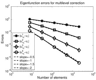
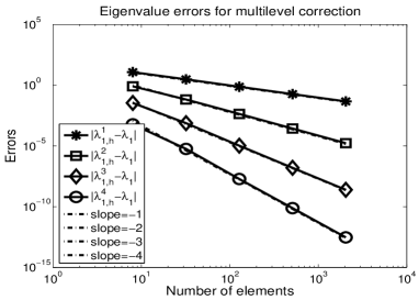
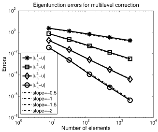
In this case, finer finite element spaces are constructed by increasing polynomial degrees of the beginning finite element space on the same mesh. We first solve the eigenvalue problem (12) by linear finite element on a relatively coarser mesh 𝒯Hsubscript𝒯𝐻\mathcal{T}_{H}, then perform the first correction step with quadratic element, followed by cubic element for the second correction step and quartic element for the third correction step. Our initial mesh 𝒯Hsubscript𝒯𝐻\mathcal{T}_{H} is obtained from the Delaunay triangulation followed by four levels of regular mesh refinement. Figure 1 depicts errors for the first eigenvalue (5/16+2π25162superscript𝜋25/16+2\pi^{2}) approximation, and Figure 2 plots numerical errors for the eigenfunction and the corresponding adjoint eigenfunction associated with the first eigenvalue.
Refer to caption
Fig. 1: Here, λh1superscriptsubscript𝜆1\lambda_{h}^{1} denote the eigenvalue approximation by linear element, λh2superscriptsubscript𝜆2\lambda_{h}^{2} is the eigenvalue approximation by the first correction with quadratic element, λh3superscriptsubscript𝜆3\lambda_{h}^{3} the eigenvalue approximation by the second correction with cubic element, λh4superscriptsubscript𝜆4\lambda_{h}^{4} the eigenvalue approximation by the third correction with quartic element
Refer to caption
Refer to caption
Fig. 2: Here, uh1superscriptsubscript𝑢1u_{h}^{1} and uh1superscriptsubscript𝑢absent1u_{*h}^{1} denote the eigenfunction approximation and its adjoint approximation by linear element, uh2superscriptsubscript𝑢2u_{h}^{2} and uh2superscriptsubscript𝑢absent2u_{*h}^{2} are eigenfunction approximation and its adjoint approximation by the first correction with quadratic element, uh3superscriptsubscript𝑢3u_{h}^{3} and uh3superscriptsubscript𝑢absent3u_{*h}^{3}, eigenfunction and its adjoint approximation by the second correction with cubic element, uh4superscriptsubscript𝑢4u_{h}^{4} and uh4superscriptsubscript𝑢absent4u_{*h}^{4}, eigenfunction and its adjoint approximation by the third correction with quartic element

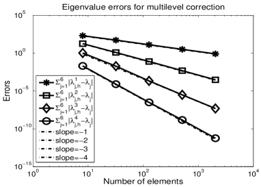
Furthermore, Figure 3 provides numerical results for the summation of the errors for the first 666 eigenvalues: 5/16+[2π2,5π2,5π2,8π2,10π2,10π2]5162superscript𝜋25superscript𝜋25superscript𝜋28superscript𝜋210superscript𝜋210superscript𝜋25/16+[2\pi^{2},5\pi^{2},5\pi^{2},8\pi^{2},10\pi^{2},10\pi^{2}].

Refer to caption
Fig. 3: Approximation errors for the summation of the errors for the first 666 eigenvalues by the multi-space way. Here, λj,h1superscriptsubscript𝜆𝑗1\lambda_{j,h}^{1} denote the eigenvalue approximation by linear element, λj,h2superscriptsubscript𝜆𝑗2\lambda_{j,h}^{2} is the eigenvalue approximation by the first correction with quadratic element, λj,h3superscriptsubscript𝜆𝑗3\lambda_{j,h}^{3} the eigenvalue approximation by the second correction with cubic element, λj,h4superscriptsubscript𝜆𝑗4\lambda_{j,h}^{4} the eigenvalue approximation by the third correction with quartic element

From Figures 1-3, we find that each correction step improves the convergence order by two for eigenvalue approximation, and by one for eigenfunction approximation when the exact eigenfunction is sufficiently smooth.

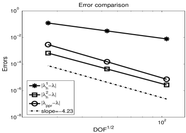
To end this subsection, we make a comparison with the PPR method [13]. We see from Figure 4 that the two-level correction scheme by the multi-space way has slightly better accuracy than the PPR method. However, the two-level correction needs to solve two extra boundary value problems while the PPR method only need to perform a local recovery at each node. Thus, we should say that the PPR method has better efficiency than the two-level correction under regular mesh refinement when the eigenfunction has regularity H3(Ω)W2,(Ω)superscript𝐻3Ωsuperscript𝑊2ΩH^{3}(\Omega)\cap W^{2,\infty}(\Omega). Nevertheless, three and four-level correction will outperform the PPR method.
Refer to caption
Fig. 4: Comparison with the PPR method in [13] when b1=10subscript𝑏110b_{1}=10 and b2=1subscript𝑏21b_{2}=1. λh1superscriptsubscript𝜆1\lambda_{h}^{1}, eigenvalue approximation by linear element; λh2superscriptsubscript𝜆2\lambda_{h}^{2}, eigenvalue approximation by the first correction with quadratic element; λpprsubscript𝜆ppr\lambda_{\rm ppr}, the eigenvalue approximation by the PPR method

5.2 Multi-grid way

An alternative way of the multilevel correction scheme is to construct finer finite element spaces by mesh refinement. We first solve the eigenvalue problem (12) in the linear finite element space on an initial coarse mesh 𝒯Hsubscript𝒯𝐻\mathcal{T}_{H} (𝒯h1:=𝒯Hassignsubscript𝒯subscript1subscript𝒯𝐻\mathcal{T}_{h_{1}}:=\mathcal{T}_{H}). Then we refine the mesh regularly with the resultant meshes 𝒯hksubscript𝒯subscript𝑘\mathcal{T}_{h_{k}} satisfying hk=21kHsubscript𝑘superscript21𝑘𝐻h_{k}=2^{1-k}H for (k=2,,n)𝑘2𝑛(k=2,\cdots,n), and solve auxiliary source problems (32) and (33) in the linear finite element space Vhksubscript𝑉subscript𝑘V_{h_{k}} defined on 𝒯hksubscript𝒯subscript𝑘\mathcal{T}_{h_{k}} and the corresponding eigenvalue problems (34) and (35) in VH,hksubscript𝑉𝐻subscript𝑘V_{H,h_{k}}. We have the following estimate

εhn(λ)subscript𝜀subscript𝑛𝜆\displaystyle\varepsilon_{h_{n}}(\lambda) =\displaystyle= k=1nHnkhk=k=1n(2H)nkhn112Hhnhn,superscriptsubscript𝑘1𝑛superscript𝐻𝑛𝑘subscript𝑘superscriptsubscript𝑘1𝑛superscript2𝐻𝑛𝑘subscript𝑛112𝐻subscript𝑛subscript𝑛\displaystyle\sum\limits_{k=1}^{n}H^{n-k}h_{k}=\sum\limits_{k=1}^{n}(2H)^{n-k}h_{n}\leq\frac{1}{1-2H}h_{n}\approx h_{n},

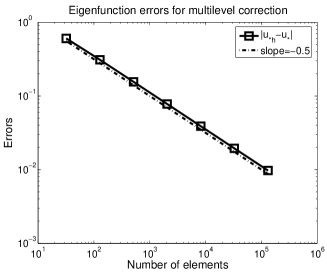
and similarly εhn(λ)hnsubscriptsuperscript𝜀subscript𝑛𝜆subscript𝑛\varepsilon^{*}_{h_{n}}(\lambda)\approx h_{n}, which implies that the multilevel correction method achieves the optimal convergence rate if the initial mesh size H𝐻H is reasonably small, say H=1/4𝐻14H=1/4 as we will use in our numerical tests.

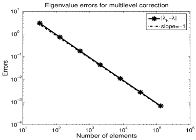
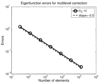
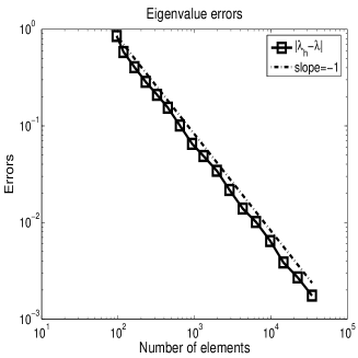
Numerical results for the first eigenvalue λ=5/16+2π2𝜆5162superscript𝜋2\lambda=5/16+2\pi^{2} and the two associated eigenfunctions are demonstrated in Figures 5 and 6, respectively. Here we use the uniform meshes with H=1/4𝐻14H=1/4.

Refer to caption
Fig. 5: Approximation errors for the first eigenvalue 5/16+2π25162superscript𝜋25/16+2\pi^{2} by the multi-grid way with H=1/4𝐻14H=1/4
Refer to caption
Refer to caption
Fig. 6: Approximation errors for the first eigenfunction and its adjoint by the multi-grid way with H=1/4𝐻14H=1/4

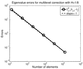
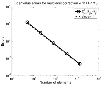
Furthermore, Figure 7 provides numerical results for the summation of the errors for the first 666 eigenvalues: 5/16+[2π2,5π2,5π2,8π2,10π2,10π2]5162superscript𝜋25superscript𝜋25superscript𝜋28superscript𝜋210superscript𝜋210superscript𝜋25/16+[2\pi^{2},5\pi^{2},5\pi^{2},8\pi^{2},10\pi^{2},10\pi^{2}] with H=1/8𝐻18H=1/8 and H=1/16𝐻116H=1/16, respectively.

Refer to caption
Refer to caption
Fig. 7: Approximation errors for the error summation of the first 666 eigenvalues by the multi-grid way with H=1/8𝐻18H=1/8 (left) and 1/161161/16 (right)

We observe from Figures 5-7, that our multilevel correction method with the multi-grid way produces eigenvalue and eigenfunction approximations with the optimal convergence rate. Therefore, we can combine the multigrid method for boundary value problems and our multilevel correction scheme (cf. [11, 18]) to achieve better efficiency for nonsymmetric eigenvalue problems.

5.3 Eigenvalue problem on L𝐿L-shape domain

In this subsection, we consider the eigenvalue problem (73) on the L𝐿L-shape domain Ω=(1,1)×(1,1)\[0,1)×(1,0]Ω\11110110\Omega=(-1,1)\times(-1,1)\backslash[0,1)\times(-1,0]. Since ΩΩ\Omega has a reentrant corner, the singularity of eigenfunctions is expected. As a consequence, the convergence rate for the first eigenvalue approximation is 4/3434/3 by the linear finite element method on quasi-uniform meshes. Since the exact eigenvalue is unknown, we choose an adequately accurate approximation λ=9.95240442893276𝜆9.95240442893276\lambda=9.95240442893276 as the exact first eigenvalue for our numerical tests.

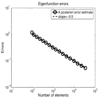
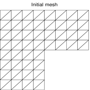
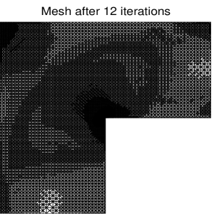
Our multilevel correction scheme is tested on a sequence of meshes 𝒯Hsubscript𝒯𝐻\mathcal{T}_{H} (𝒯h1:=𝒯Hassignsubscript𝒯subscript1subscript𝒯𝐻\mathcal{T}_{h_{1}}:=\mathcal{T}_{H}), 𝒯h2,,𝒯hnsubscript𝒯subscript2subscript𝒯subscript𝑛\mathcal{T}_{h_{2}},\cdots,\mathcal{T}_{h_{n}} produced by the adaptive refinement (cf. [17, 24]). Here the ZZ recovery method (cf. [26]) is adopted as the a posteriori error estimator for eigenfunction and adjoint eigenfunction approximations uhua,h2+uhua,h2superscriptsubscriptnormsubscript𝑢𝑢𝑎2superscriptsubscriptnormsuperscriptsubscript𝑢superscript𝑢𝑎2\sqrt{\|u_{h}-u\|_{a,h}^{2}+\|u_{h}^{*}-u^{*}\|_{a,h}^{2}}. Figure 8 shows the initial mesh and the mesh after 121212 adaptive iterations. Figure 9 gives the corresponding numerical results for the adaptive iterations.
Refer to caption
Refer to caption
Fig. 8: The initial mesh and the one after 12 adaptive iterations for the L-shape domain
Refer to caption
Refer to caption
Fig. 9: Approximation errors of the first eigenvalue and the a posteriori errors of the associated eigenfunction and adjoint eigenfunction

From Figure 9, we observe that the multilevel correction method works well on adaptive meshes with the optimal convergence rate. Furthermore, the situation is very different from the two-gird [9, 23, 25] method in that the initial mesh has very little impact on the finest one. Thus the multilevel correction method can be coupled with the adaptive refinement naturally.

5.4 Eigenvalue problem with complex vector

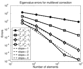
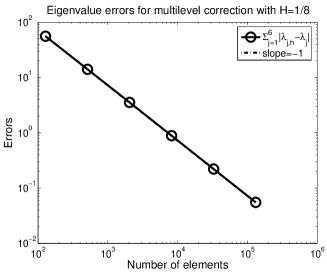
In this subsection, we test the multilevel correction scheme for the problem (73) with complex vector 𝐛=[1+2i,1/2i]T𝐛superscript12i12i𝑇\mathbf{b}=[1+2\textrm{i},1/2-\textrm{i}]^{T}. We use the multi-space and multi-grid ways as in Subsections 5.1 and 5.2, respectively, to check the multilevel correction scheme. Figure 10 shows the numerical results for the first 666 eigenvalues. It is observed from Figure 10 that the multilevel correction method defined in Algorithm 4.1 can also work very well for the nonsymmetric eigenvalue problems with complex vector.
Refer to caption
Refer to caption
Fig. 10: Approximation errors for the summation of errors for the first 666 eigenvalues by the multi-space way (left) and the multi-grid way with H=1/8𝐻18H=1/8 (right). Here, λj,h1superscriptsubscript𝜆𝑗1\lambda_{j,h}^{1} denote the eigenvalue approximation by linear element, λj,h2superscriptsubscript𝜆𝑗2\lambda_{j,h}^{2} is the eigenvalue approximation by the first correction with quadratic element, λj,h3superscriptsubscript𝜆𝑗3\lambda_{j,h}^{3} the eigenvalue approximation by the second correction with cubic element, λj,h4superscriptsubscript𝜆𝑗4\lambda_{j,h}^{4} the eigenvalue approximation by the third correction with quartic element

6 Concluding remarks

In this paper, we propose and analyze a multilevel correction scheme to improve the efficiency of both defective and nondefective nonsymmetric eigenpair approximations. In this multilevel correction, we only need to solve eigenvalue problems in the coarsest finite element space. Sometimes, we also need to compute the algebraic eigenspace based on the geometric eigenspace when the ascent is larger than 111.

Furthermore, our multilevel correction scheme can be coupled with the multigrid method to construct a parallel method for eigenvalue problems (see, e.g, [11, 12, 18, 24]). It can also be combined with adaptive techniques (cf. [17]) for singular eigenfunction cases. These will be our future work.

A final remark. As long as higher eigenvalues are concerned, the multi-space way is preferred (than the multi-grid way). We can see it clearly by comparing numerical accuracies for summations of the first 6 eigenvalues in §5.1 and §5.2.

Acknowledgments

The first author is supported in part by the National Natural Science Foundation of China (NSFC 91330202, 11001259, 11371026, 11201501, 11031006, 2011CB309703) and the National Center for Mathematics and Interdisciplinary Science, CAS and the President Foundation of AMSS-CAS. The second author is supported in part by the US National Science Foundation through grant DMS-1115530, DMS-1419040, and the National Natural Science Foundation of China (91430216, 11471031).

References

  • [1] K. A. Cliffe, E. J. C. Hall and P. Houston, Adaptive discontinuous Galerkin methods for eigenvalue problems arising in incompressible fluid flows, SIAM J. Sci. Comput., 31(6) (2010), pp. 4607-4632.
  • [2] I. Babuška and J. E. Osborn, Finite element-Galerkin approximation of the eigenvalues and eigenvectors of selfadjoint problems, Math. Comp. 52 (1989), pp. 275-297.
  • [3] I. Babuška and J. Osborn, Eigenvalue Problems, In Handbook of Numerical Analysis, Vol. II, (Eds. P. G. Lions and Ciarlet P.G.), Finite Element Methods (Part 1), North-Holland, Amsterdam, pp. 641-787, 1991.
  • [4] S. Brenner and L. Scott, The Mathematical Theory of Finite Element Methods, New York: Springer-Verlag, 1994.
  • [5] F. Chatelin, Spectral Approximation of Linear Operators, Academic Press Inc, New York, 1983.
  • [6] P. G. Ciarlet, The finite Element Method for Elliptic Problem, North-holland Amsterdam, 1978.
  • [7] V. Heuveline and R. Rannacher, A posteriori error control for finite element app. roximations of elliptic eigenvalue problems, Adv. Comput. Math., 15 (2001), pp. 107-138.
  • [8] V. Heuveline and R. Rannacher, Adaptive FEM for eigenvalue problems with application in hydrodynamic stability analysis, J. Numer. Math., submitted, 2006.
  • [9] K. Kolman, A two-level method for Nonsymmetric eigenvalue problems, Acta Mathematicae App. licatae Sinica (English series), 2(1) (2005), pp. 1-12.
  • [10] Q. Lin, F. Luo and H. Xie, A multilevel correction method for Stokes eigenvalue problems and its applications, Math. Methods Appl. Sci., DOI: 10.1002/mma.2866, 2013.
  • [11] Q. Lin and H. Xie, A multi-level correction scheme for eigenvalue problems, Math. Comp., DOI: http://dx.doi.org/10.1090/S0025-5718-2014-02825-1, 2014.
  • [12] Q. Lin and H. Xie, A type of multigrid method for eigenvalue problem, Research Report in ICMSEC, 2011-06 (2011).
  • [13] A. Naga and Z. Zhang, Function value recovery and its appplication in eigenvalue problems, SIAM J. Numer. Anal., 50(1) (2012), pp. 272-286.
  • [14] A. Naga, Z. Zhang and A. Zhou, Enhancing eigenvalue app. roximation by gradient recovery, SIAM J. Sci. Comput., 28(4) (2006), pp. 1289-1300.
  • [15] P. Schmid and D. S. Henningson, Stability and Transition in Shear Flows, Appl. Math. Sci. 142, Springer, New York, 2001.
  • [16] V. Shaidurov, Multigrid methods for finite element, Kluwer Academic Publics, Netherlands, 1995.
  • [17] H. Wu and Z. Zhang, Enhancing eigenvalue app. roximation by gradient recovery on adaptive meshes, IMA J. Numer. Anal., 29(4) (2009), pp. 1008-1022.
  • [18] H. Xie, A type of multilevel method for the Steklov eigenvalue problem, IMA J. Numer. Anal., 1-17, doi:10.1093/imanum/drt009, 2013.
  • [19] H. Xie, A multigrid method for eigenvalue problem, J. Comput. Phys., 274 (2014), 550-561.
  • [20] J. Xu, Iterative methods by space decomposition and subspace correction, SIAM Review, 34(4) (1992), pp. 581-613.
  • [21] J. Xu, A new class of iterative methods for nonselfadjoint or indefinite problems, SIAM J. Numer. Anal., 29 (1992), pp. 303-319.
  • [22] J. Xu, A novel two-grid method for semilinear elliptic equations, SIAM J. Sci. Comput., 15 (1994), pp. 231-237.
  • [23] J. Xu and A. Zhou, A two-grid discretization scheme for eigenvalue problems, Math. Comput., 70(233) (2001), 17-25.
  • [24] J. Xu and A. Zhou, Local and parallel finite element algorithm for eigenvalue problems, Acta Math. App. l. Sin. Engl. Ser., 18(2) (2002), pp. 185-200.
  • [25] Y. Yang and X. Fan, Generalized Rayleigh quotient and finite element two-grid discretization schemes, Science in China Series A: mathematics, 52(9) (2009), pp. 1955-1972.
  • [26] O. Zienkiewicz and J. Zhu, A simple error estimator and adaptive procedure for practical engineering analysis, Int. J. Numer. Methods Eng., 24 (1987), pp. 337-357.