Two-Dimensional Pattern-Coupled Sparse Bayesian Learning via Generalized Approximate Message Passing

Abstract

We consider the problem of recovering two-dimensional (2-D) block-sparse signals with unknown cluster patterns. Two-dimensional block-sparse patterns arise naturally in many practical applications such as foreground detection and inverse synthetic aperture radar imaging. To exploit the block-sparse structure, we introduce a 2-D pattern-coupled hierarchical Gaussian prior model to characterize the statistical pattern dependencies among neighboring coefficients. Unlike the conventional hierarchical Gaussian prior model where each coefficient is associated independently with a unique hyperparameter, the pattern-coupled prior for each coefficient not only involves its own hyperparameter, but also its immediate neighboring hyperparameters. Thus the sparsity patterns of neighboring coefficients are related to each other and the hierarchical model has the potential to encourage 2-D structured-sparse solutions. An expectation-maximization (EM) strategy is employed to obtain the maximum a posterior (MAP) estimate of the hyperparameters, along with the posterior distribution of the sparse signal. In addition, the generalized approximate message passing (GAMP) algorithm is embedded into the EM framework to efficiently compute an approximation of the posterior distribution of hidden variables, which results in a significant reduction in computational complexity. Numerical results are provided to illustrate the effectiveness of the proposed algorithm.

I Introduction

Compressed sensing is a recently emerged technique for signal sampling and data acquisition which enables to recover sparse signals from undersampled linear measurements

$$\boldsymbol{y}=\boldsymbol{Ax}+\boldsymbol{w}$$ (1)

where $\boldsymbol{A}\in\mathbb{R}^{M\times N}$ is a sampling matrix with $M\ll N$, $\boldsymbol{x}$ denotes an $N$-dimensional sparse signal, and $\boldsymbol{w}$ denotes the additive noise. The problem has been extensively studied and a variety of algorithms, e.g. the orthogonal matching pursuit (OMP) algorithm [1], the basis pursuit (BP) method [2], the iterative reweighted $\ell_{1}$ and $\ell_{2}$ algorithms [3], and the sparse Bayesian learning method [4, 5, 6] were proposed. In many practical applications, in addition to the sparse structure, sparse signals may exhibit two-dimensional cluster patterns that can be utilized to enhance the recovery performance. For example, the target of interest in the synthetic aperture radar/inverse synthetic aperture radar (SAR/ISAR) images often demonstrates continuity in both the range and cross-range domains [7]. In video surveillance, the foreground image exhibits a cluster pattern since the foreground objects (humans, cars, text etc.) generally occupy a small continuous region of the scene [8]. Besides these, block-sparsity is also present in temporal observations of a time-varying block-sparse signal whose support varies slowly over time [9].

Analyses [10, 11, 12] show that exploiting the inherent block-sparse structure not only leads to relaxed conditions for exact reconstruction, but also helps improve the recovery performance considerably. A number of algorithms have been proposed for recovering block-sparse signals over the past few years, e.g., block-OMP [12], mixed $\ell_{2}/\ell_{1}$ norm-minimization [10], group LASSO [13], model-based CoSaMP [11], and block-sparse Bayesian learning [14, 15]. These algorithms, however, require a priori knowledge of the block partition (e.g. the number of blocks and location of each block) such that the coefficients in each block are grouped together and enforced to share a common sparsity pattern. In practice, the prior information about the block partition of sparse signals is often unavailable, especially for two-dimensional signals since the block partition of a two-dimensional signal involves not only the location but also the shape of each block. For example, foreground images have irregular and unpredictable cluster patterns which are very difficult to be estimated a priori. To address this difficulty, a few sophisticated Bayesian methods which do not need the knowledge of the block partition were developed. In [16], a “spike-and-slab” prior model was proposed, where by introducing dependencies among mixing weights, the prior model has the potential to encourage sparsity and promote a tree structure simultaneously. This “spike-and-slab” prior model was later extended to accommodate block-sparse signals [17, 7]. Nevertheless, for the “spike-and-slab” prior introduced in [16, 17], the posterior distribution cannot be derived analytically, and a Markov chain Monte Carlo (MCMC) sampling method has to be employed for Bayesian inference. In [18, 19], a graphical prior, also referred to as the “Boltzmann machine”, is employed as a prior on the sparsity support in order to induce statistical dependencies between atoms. With such a prior, the maximum a posterior (MAP) estimator requires an exhaustive search over all possible sparsity patterns. To overcome the intractability of the combinatorial search, a greedy method [18] and a variational mean-field approximation method [19] were developed to approximate the MAP. In [20], to cope with the unknown cluster pattern, an expanded model is employed by assuming that the original sparse signal is a superposition of a number of overlapping blocks, and the coefficients in each block share the same sparsity pattern. Conventional block sparse Bayesian learning algorithms such as those in [15] can then be applied to the expanded model.

Recently in [21], we proposed a pattern-coupled hierarchical Gaussian prior model to exploit the unknown block-sparse structure. Unlike the conventional hierarchical Gaussian prior model [4, 5, 6] where each coefficient is associated independently with a unique hyperparameter, the pattern-coupled prior for each coefficient not only involves its own hyperparameter, but also its immediate neighboring hyperparameters. This pattern-coupled hierarchical model is effective and flexible to capture any underlying block-sparse structures, without requiring the prior knowledge of the block partition. Numerical results show that the pattern-coupled sparse Bayesian learning (PC-SBL) method renders competitive performance for block-sparse signal recovery. Nevertheless, a major drawback of the method is that it requires computing an $N\times N$ matrix inverse at each iteration, and thus has a cubic complexity in terms of the signal dimension. This high computational cost prohibits its application to problems with even moderate dimensions. Also, [21] only considers recovery of one-dimensional block-sparse signals. In this paper, we generalize the pattern-coupled hierarchical model to the two-dimensional (2-D) scenario in order to leverage block-sparse patterns arising from 2-D sparse signals. To address the computational issue, we resort to the generalized approximate message passing (GAMP) technique [22] and develop a computationally efficient method. Specifically, the algorithm is developed within an expectation-maximization (EM) framework, using the GAMP to efficiently compute an approximation of the posterior distribution of hidden variables. The hyperparameters associated with the hierarchical Gaussian prior are learned by iteratively maximizing the Q-function which is calculated based on the posterior approximation obtained from the GAMP. Simulation results show that the proposed method presents superior recovery performance for block-sparse signals, meanwhile achieving a significant reduction in computational complexity.

The rest of the paper is organized as follows. In Section II, we introduce a 2-D pattern coupled hierarchical Gaussian framework to model the sparse prior and the pattern dependencies among the neighboring coefficients. In Section III, a GAMP-based EM algorithm is developed to obtain the maximum a posterior (MAP) estimate of the hyperparameters, along with the posterior distribution of the sparse signal. Simulation results are provided in Section IV, followed by concluding remarks in Section V.

II Bayesian Model

We consider the problem of recovering a two-dimensional block-sparse signal $\boldsymbol{X}\in\mathbb{R}^{Q\times L}$ from compressed noisy measurements

$$\boldsymbol{y}=\boldsymbol{f}(\boldsymbol{X})+\boldsymbol{w}$$ (2)

where $\boldsymbol{y}\in\mathbb{R}^{M}$ denotes the compressed measurement vector, $\boldsymbol{f}(\cdot)$ is a linear map: $\mathbb{R}^{Q\times L}\rightarrow\mathbb{R}^{M}$, with $M\ll N\triangleq QL$, and $\boldsymbol{w}\in\mathbb{R}^{M}$ is an additive multivariate Gaussian noise with zero mean and covariance matrix $\sigma^{2}\boldsymbol{I}$. Let $\boldsymbol{x}\triangleq\text{vec}(\boldsymbol{X})$, the linear map $\boldsymbol{f}(\boldsymbol{X})$ can generally be expressed as

$$\boldsymbol{f}(\boldsymbol{X})=\boldsymbol{A}\boldsymbol{x}$$ (3)

where $\boldsymbol{A}\in\mathbb{R}^{M\times N}$ denotes the measurement matrix. In the special case where $\boldsymbol{f}(\boldsymbol{X})=\text{vec}(\boldsymbol{BX})$, then we have $\boldsymbol{A}\triangleq\boldsymbol{I}\otimes\boldsymbol{B}$, in which $\otimes$ stands for the Kronecker product. The above model (2) arises in image applications where signals are multi-dimensional in nature, or in the scenario where multiple snapshots of a time-varying sparse signal are available. In these applications, signals usually exhibit two-dimensional cluster patterns that can be utilized to improve the recovery accuracy. To leverage the underlying block-sparse structures, we introduce a 2-D pattern-coupled Gaussian prior model which is a generalization of our previous work [21]. Before proceeding, we provide a brief review of the conventional hierarchical Gaussian prior model [4], and some of its extensions.

II-A Review of Conventional Gaussian Prior Model

For ease of exposition, we consider the prior model for the two-dimensional signal $\boldsymbol{X}$ instead of its one-dimensional form $\boldsymbol{x}$. Let $x_{q,l}$ denote the $(q,l)$th entry of $\boldsymbol{X}$. In the conventional sparse Bayesian learning framework [4], a two-layer hierarchical Gaussian prior was employed to promote the sparsity of the solution. In the first layer, coefficients $\{x_{q,l}\}$ of $\boldsymbol{X}$ are assigned a Gaussian prior distribution

$$p(\boldsymbol{X}|\boldsymbol{\alpha})=\prod_{q=1}^{Q}\prod_{l=1}^{L}\mathcal{N}(x_{q,l}|0,\alpha_{q,l}^{-1})$$ (4)

where $\alpha_{q,l}$ is a non-negative hyperparameter controlling the sparsity of the coefficient $x_{q,l}$. The second layer specifies Gamma distributions as hyperpriors over the hyperparameters $\boldsymbol{\alpha}\triangleq\{\alpha_{q,l}\}$, i.e.

$$p(\boldsymbol{\alpha})=\prod_{q=1}^{Q}\prod_{l=1}^{L}\text{Gamma}(\alpha_{q,l}|a,b)$$ (5)

As discussed in [4], for properly chosen $a$ and $b$, this hyperprior allows the posterior mean of $\alpha_{q,l}$ to become arbitrarily large. As a consequence, the associated coefficient $x_{q,l}$ will be driven to zero, thus yielding a sparse solution. This conventional hierarchical model, however, does not encourage structured-sparse solutions since the sparsity of each coefficient is determined by its own hyperparameter and the hyperparameters are independent of each other. In [14, 15], the above hierarchical model was generalized to deal with block-sparse signals, in which a group of coefficients sharing the same sparsity pattern are assigned a multivariate Gaussian prior parameterized by a common hyperparameter. Nevertheless, this model requires the knowledge of the block partition to determine which coefficients should be grouped and assigned a common hyperparameter.

II-B Proposed 2-D Pattern-Coupled Hierarchical Model

To exploit the 2-D block-sparse structure, we utilize the fact that the sparsity patterns of neighboring coefficients are statistically dependent. To capture the pattern dependencies among neighboring coefficients, the Gaussian prior for each coefficient $x_{q,l}$ not only involves its own hyperparameter $\alpha_{q,l}$, but also its immediate neighbor hyperparameters. Specifically, a prior over $\boldsymbol{X}$ is given by

$$p(\boldsymbol{X}|\boldsymbol{\alpha})=\prod_{q=1}^{Q}\prod_{l=1}^{L}\mathcal{N}(x_{q,l}|0,\delta_{q,l}^{-1})$$ (6)

where

$$\delta_{q,l}\triangleq\alpha_{q,l}+\beta\sum_{(i,j)\in N_{(q,l)}}\alpha_{i,j}$$ (7)

in which $N_{(q,l)}$ denotes the neighborhood of the grid point $(q,l)$, i.e. $N_{(q,l)}\triangleq\{(q,l-1),(q,l+1),(q-1,l),(q+1,l)\}$, and $\beta\in[0,1]$ is a parameter indicating the pattern relevance between the coefficient $x_{q,l}$ and its neighboring coefficients. Clearly, this model is an extension of our previous prior model [21] to the two-dimensional case. When $\beta=0$, the prior model (6) reduces to the conventional sparse Bayesian learning model. When $\beta>0$, we see that the sparsity of each coefficient $x_{q,l}$ is not only controlled by the hyperparameter $\alpha_{q,l}$, but also by the neighboring hyperparameters $S_{\alpha_{q,l}}\triangleq\{\alpha_{i,j}|(i,j)\in N_{(q,l)}\}$. The coefficient $x_{q,l}$ will be driven to zero if $\alpha_{q,l}$ or any of its neighboring hyperparameters goes to infinity. In other words, suppose $\alpha_{q,l}$ approaches infinity, then not only its corresponding coefficient $x_{q,l}$ will be driven to zero, the neighboring coefficients $S_{x_{q,l}}\triangleq\{x_{i,j}|(i,j)\in N_{(q,l)}\}$ will decrease to zero as well. We see that the sparsity patterns of neighboring coefficients are related to each other through their shared hyperparameters. On the other hand, for any pair of neighboring coefficients, each of them has its own hyperparameters that are not shared by the other coefficient. Hence, no coefficients are pre-specified to share a common sparsity pattern, which enables the prior to provide flexibility to model any block-sparse structures.

Following [4], we use Gamma distributions as hyperpriors over the hyperparameters $\{\alpha_{q,l}\}$, i.e.

$$p(\boldsymbol{\alpha})=\prod_{q=1}^{Q}\prod_{l=1}^{L}\text{Gamma}(\alpha_{q,l}|a,b)$$ (8)

where we set $a>1$, and $b=10^{-6}$. The choice of $a$ will be elaborated later in our paper. Also, the noise variance $\sigma^{2}\triangleq 1/\gamma$ is assumed unknown, and to estimate this parameter, we place a Gamma hyperprior over $\gamma$, i.e.

$$p(\gamma)=\text{Gamma}(\gamma|c,d)$$ (9)

where we set $c=1$ and $d=10^{-6}$.

III Proposed Algorithm

We now proceed to perform Bayesian inference for the proposed pattern-coupled hierarchical model. The following model is considered since the linear map $\boldsymbol{f}(\boldsymbol{X})$ can be expressed as $\boldsymbol{f}(\boldsymbol{X})=\boldsymbol{A}\boldsymbol{x}$

$$\boldsymbol{y}=\boldsymbol{A}\boldsymbol{x}+\boldsymbol{w}$$ (10)

We first translate the prior for the two-dimensional signal $\boldsymbol{X}$ to a prior for its one-dimensional form $\boldsymbol{x}$. From (6), the prior over $\boldsymbol{x}$ can be expressed as

$$p(\boldsymbol{x}|\boldsymbol{\alpha})=\prod_{n=1}^{N}\mathcal{N}(x_{n}|0,\eta_{n}^{-1})$$ (11)

where

$$\eta_{n}\triangleq\alpha_{n}+\beta\sum_{i\in N_{(n)}}\alpha_{i}$$ (12)

in which $N_{(n)}$ denotes the neighbors of the point $(q,l)$ on the two-dimensional grid, i.e. $N_{(n)}\triangleq\{(l-2)Q+q,lQ+q,(l-1)Q+q-1,(l-1)Q+q+1\}$. The relation between $n$ and $(q,l)$ is given by $n=(l-1)Q+q$, that is, $l=\lceil n/Q\rceil$, and $q=n\phantom{0}\text{mod}\phantom{0}Q$, in which $\lceil\cdot\rceil$ denotes the ceiling operator. Note that for notational convenience, we, with a slight abuse of notation, use $x_{n}$ to denote the $n$th entry of $\boldsymbol{x}$ and $\alpha_{n}$ to denote the hyperparameter associated with the coefficient $x_{n}$. Also, let $\boldsymbol{\alpha}\triangleq\{\alpha_{n}\}$ since its exact meaning remains unaltered. From (8), we have

$$p(\boldsymbol{\alpha})=\prod_{n=1}^{N}\text{Gamma}(\alpha_{n}|a,b)$$ (13)

An expectation-maximization (EM) algorithm can be developed for learning the sparse signal $\boldsymbol{x}$ as well as the hyperparameters $\{\boldsymbol{\alpha},\gamma\}$. In the EM formulation, the signal $\boldsymbol{x}$ is treated as hidden variables, and we iteratively maximize a lower bound on the posterior probability $p(\boldsymbol{\alpha},\gamma|\boldsymbol{y})$ (this lower bound is also referred to as the Q-function). Briefly speaking, the algorithm alternates between an E-step and a M-step. In the E-step, we need to compute the posterior distribution of $\boldsymbol{x}$ conditioned on the observed data and the hyperparameters estimated from the $t$th iteration, i.e.

$$p(\boldsymbol{x}|\boldsymbol{y},\boldsymbol{\alpha}^{(t)},\gamma^{(t)})\propto p(\boldsymbol{x}|\boldsymbol{\alpha}^{(t)})p(\boldsymbol{y}|\boldsymbol{x},\gamma^{(t)})$$ (14)

It can be readily verified that the posterior $p(\boldsymbol{x}|\boldsymbol{y},\boldsymbol{\alpha}^{(t)},\gamma^{(t)})$ follows a Gaussian distribution with its mean and covariance matrix given respectively by

$$\boldsymbol{\mu}= \gamma^{(t)}\boldsymbol{\Phi}\boldsymbol{A}^{T}\boldsymbol{y}$$ (15)

$$\boldsymbol{\Phi}= (\gamma^{(t)}\boldsymbol{A}^{T}\boldsymbol{A}+\boldsymbol{D})^{-1}$$ (16)

where $\boldsymbol{D}\triangleq\text{diag}(\eta_{1}^{(t)},\ldots,\eta_{N}^{(t)})$. The Q-function, i.e. $E_{\boldsymbol{x}|\boldsymbol{y},\boldsymbol{\alpha}^{(t)},\gamma^{(t)}}[\log p(\boldsymbol{\alpha},\gamma|\boldsymbol{y})]$, can then be computed, where the operator $E_{\boldsymbol{x}|\boldsymbol{y},\boldsymbol{\alpha}^{(t)},\gamma^{(t)}}[\cdot]$ denotes the expectation with respect to the posterior distribution $p(\boldsymbol{x}|\boldsymbol{y},\boldsymbol{\alpha}^{(t)},\gamma^{(t)})$. In the M-step, we maximize the Q-function with respect to the hyperparameters $\{\boldsymbol{\alpha},\gamma\}$.

It can be seen that the EM algorithm, at each iteration, requires to update the posterior distribution $p(\boldsymbol{x}|\boldsymbol{y},\boldsymbol{\alpha}^{(t)},\gamma^{(t)})$, which involves computing an $N\times N$ matrix inverse. Thus the EM-based algorithm has a computational complexity of $\mathcal{O}(N^{3})$ flops, and therefore is not suitable for many real-world applications involving large dimensions. In the following, we will develop a computationally efficient algorithm by resorting to the generalized approximate message passing (GAMP) technique [22]. GAMP is a very-low-complexity Bayesian iterative technique recently developed [22] for obtaining an approximation of the posterior distribution $p(\boldsymbol{x}|\boldsymbol{y},\boldsymbol{\alpha}^{(t)},\gamma^{(t)})$. It therefore can naturally be embedded within the EM framework to replace the computation of the true posterior distribution. From GAMP’s point of view, the hyperparameters $\{\boldsymbol{\alpha},\gamma\}$ are considered as known. The hyperparameters can be updated in the M-step based on the approximate posterior distribution of $\boldsymbol{x}$. We now proceed to derive the GAMP algorithm for the pattern-coupled Gaussian hierarchical prior model.

III-A Pattern-Coupled Hierarchical Gaussian GAMP

GAMP was developed in a message passing-based framework. By using central-limit-theorem approximations, message passing between variable nodes and factor nodes can be greatly simplified, and the loopy belief propagation on the underlying factor graph can be efficiently performed. As noted in [23, 22], the central-limit-theorem approximations become exact in the large-system limit under i.i.d. zero-mean sub-Gaussian $\boldsymbol{A}$.

For notational convenience, let $\boldsymbol{\theta}\triangleq\{\boldsymbol{\alpha},\gamma\}$ denote the hyperparameters. Firstly, GAMP assumes posterior independence among hidden variables $\{x_{n}\}$ and approximates the true posterior distribution $p(x_{n}|\boldsymbol{y},\boldsymbol{\theta})$ by

$$\hat{p}(x_{n}|\boldsymbol{y},\hat{r}_{n},\tau_{n}^{r},\boldsymbol{\theta})= \frac{p(x_{n}|\boldsymbol{\theta})\mathcal{N}(x_{n}|\hat{r}_{n},\tau_{n}^{r})}{\int_{x}p(x_{n}|\boldsymbol{\theta})\mathcal{N}(x_{n}|\hat{r}_{n},\tau_{n}^{r})}$$ (17)

where $\hat{r}_{n}$ and $\tau_{n}^{r}$ are quantities iteratively updated during the iterative process of the GAMP algorithm. Here, we have dropped their explicit dependence on the iteration number $k$ for simplicity. Substituting (11) into (17), it can be easily verified that the approximate posterior $\hat{p}(x_{n}|\boldsymbol{y},\hat{r}_{n},\tau_{n}^{r},\boldsymbol{\theta})$ follows a Gaussian distribution with its mean and variance given respectively as

$$\mu_{n}^{x} \triangleq\frac{\hat{r}_{n}}{1+\eta_{n}\tau_{n}^{r}}$$ (18)

$$\phi_{n}^{x} \triangleq\frac{\tau_{n}^{r}}{1+\eta_{n}\tau_{n}^{r}}$$ (19)

Another approximation is made to the noiseless output $z_{m}\triangleq\boldsymbol{a}_{m}^{T}\boldsymbol{x}$, where $\boldsymbol{a}_{m}^{T}$ denotes the $m$th row of $\boldsymbol{A}$. GAMP approximates the true marginal posterior $p(z_{m}|\boldsymbol{y},\boldsymbol{\theta})$ by

$$\hat{p}(z_{m}|\boldsymbol{y},\hat{p}_{m},\tau_{m}^{p},\boldsymbol{\theta})=\frac{p(y_{m}|z_{m},\boldsymbol{\theta})\mathcal{N}(z_{m}|\hat{p}_{m},\tau_{m}^{p})}{\int_{z}p(y_{m}|z_{m},\boldsymbol{\theta})\mathcal{N}(z_{m}|\hat{p}_{m},\tau_{m}^{p})}$$ (20)

where $\hat{p}_{m}$ and $\tau_{m}^{p}$ are quantities iteratively updated during the iterative process of the GAMP algorithm. Again, here we dropped their explicit dependence on the iteration number $k$. Under the additive white Gaussian noise assumption, we have $p(y_{m}|z_{m},\boldsymbol{\theta})=\mathcal{N}(y_{m}|z_{m},1/\gamma)$. Thus $\hat{p}(z_{m}|\boldsymbol{y},\hat{p}_{m},\tau_{m}^{p},\boldsymbol{\theta})$ also follows a Gaussian distribution with its mean and variance given by

$$\mu_{m}^{z}\triangleq \frac{\tau_{m}^{p}\gamma y_{m}+\hat{p}_{m}}{1+\gamma\tau_{m}^{p}}$$ (21)

$$\phi_{m}^{z}\triangleq \frac{\tau_{m}^{p}}{1+\gamma\tau_{m}^{p}}$$ (22)

With the above approximations, we can now define the following two scalar functions: $g_{\text{in}}(\cdot)$ and $g_{\text{out}}(\cdot)$ that are used in the GAMP algorithm. The input scalar function $g_{\text{in}}(\cdot)$ is simply defined as the posterior mean $\mu_{n}^{x}$ [22], i.e.

$$g_{\text{in}}(\hat{r}_{n},\tau_{n}^{r},\boldsymbol{\theta})=\mu_{n}^{x}=\frac{\hat{r}_{n}}{1+\eta_{n}\tau_{n}^{r}}$$ (23)

The scaled partial derivative of $\tau_{n}^{r}g_{\text{in}}(\hat{r}_{n},\tau_{n}^{r},\boldsymbol{\theta})$ with respect to $\hat{r}_{n}$ is the posterior variance $\phi_{n}^{x}$, i.e.

$$\tau_{n}^{r}\frac{\partial}{\partial\hat{r}_{n}}g_{\text{in}}(\hat{r}_{n},\tau_{n}^{r},\boldsymbol{\theta})=\phi_{n}^{x}=\frac{\tau_{n}^{r}}{1+\eta_{n}\tau_{n}^{r}}$$ (24)

The output scalar function $g_{\text{out}}(\cdot)$ is related to the posterior mean $\mu_{m}^{z}$ as follows

$$g_{\text{out}}(\hat{p}_{m},\tau_{m}^{p},\boldsymbol{\theta})=\frac{1}{\tau_{m}^{p}}(\mu_{m}^{z}-\hat{p}_{m})=\frac{1}{\tau_{m}^{p}}\bigg{(}\frac{\tau_{m}^{p}\gamma y_{m}+\hat{p}_{m}}{1+\gamma\tau_{m}^{p}}-\hat{p}_{m}\bigg{)}$$ (25)

The partial derivative of $g_{\text{out}}(\hat{p}_{m},\tau_{m}^{p},\boldsymbol{\theta})$ is related to the posterior variance $\phi_{m}^{z}$ in the following way

$$\tau_{m}^{p}\frac{\partial}{\partial\hat{p}_{m}}g_{\text{out}}(\hat{p}_{m},\tau_{m}^{p},\boldsymbol{\theta})=\frac{\phi_{m}^{z}-\tau_{m}^{p}}{\tau_{m}^{p}}=\frac{-\gamma\tau_{m}^{p}}{1+\gamma\tau_{m}^{p}}$$ (26)

Given the above definitions of $g_{\text{in}}(\cdot)$ and $g_{\text{out}}(\cdot)$, the GAMP algorithm tailored to the considered sparse signal estimation problem can now be summarized as follows (details of the derivation of the GAMP algorithm can be found in [22]), in which $a_{mn}$ denotes the $(m,n)$th entry of $\boldsymbol{A}$, $\mu_{n}^{x}(k)$ and $\phi_{n}^{x}(k)$ denote the posterior mean and variance of $x_{n}$ at iteration $k$, respectively.

GAMP Algorithm
Initialization: given $\boldsymbol{\theta}^{(t)}$; set $k=0$, $\hat{s}_{m}^{(-1)}=0,\forall m\in\{1,\ldots,M\}$; $\{\mu_{n}^{x}(k)\}_{n=1}^{N}$ and $\{\phi_{n}^{x}(k)\}_{n=1}^{N}$ are initialized as the mean and variance of the prior distribution.
Repeat the following steps until $\sum_{n}|\mu_{n}^{x}(k+1)-\mu_{n}^{x}(k)|^{2}\leq\epsilon$, where $\epsilon$ is a pre-specified error tolerance.
Step 1. $\forall m\in\{1,\ldots,M\}$:
$\begin{aligned} \qquad\qquad\quad\hat{z}_{m}(k)=&\sum_{n}a_{mn}\mu_{n}^{x}(k)\\ \tau_{m}^{p}(k)=&\sum_{n}a_{mn}^{2}\phi_{n}^{x}(k)\\ \hat{p}_{m}(k)=&\hat{z}_{m}(k)-\tau_{m}^{p}(k)\hat{s}_{m}(k-1)\\ \end{aligned}$
Step 2. $\forall m\in\{1,\ldots,M\}$:
$\begin{aligned} \qquad\qquad\quad\hat{s}_{m}(k)=&g_{\text{out}}(\hat{p}_{m}(k),\tau^{p}_{m}(k),\boldsymbol{\theta}^{(t)})\\ \tau^{s}_{m}(k)=&-\frac{\partial}{\partial\hat{p}_{m}}g_{\text{out}}(\hat{p}_{m}(k),\tau^{p}_{m}(k),\boldsymbol{\theta}^{(t)})\\ \end{aligned}$
Step 3. $\forall n\in\{1,\ldots,N\}$:
$\begin{aligned} \qquad\qquad\quad\tau_{n}^{r}(k)=&\left(\sum_{m}a_{mn}^{2}\tau^{s}_{m}(k)\right)^{-1}\\ \hat{r}_{n}(k)=&\mu_{n}^{x}(k)+\tau_{n}^{r}(k)\sum_{m}a_{mn}\hat{s}_{m}(k)\\ \end{aligned}$
Step 4. $\forall n\in\{1,\ldots,N\}$:
$\begin{aligned} \qquad\qquad\quad\mu_{n}^{x}(k+1)=&g_{\text{in}}(\hat{r}_{n}(k),\tau_{n}^{r}(k),\boldsymbol{\theta}^{(t)})\\ \phi_{n}^{x}(k+1)=&\tau_{n}^{r}(k)\frac{\partial}{\partial\hat{r}_{n}}g_{\text{in}}(\hat{r}_{n}(k),\tau_{n}^{r}(k),\boldsymbol{\theta}^{(t)})\\ \end{aligned}$
Output: $\{\hat{r}_{n}(k_{0}),\tau_{n}^{r}(k_{0})\}$, $\{\hat{p}_{m}(k_{0}),\tau_{m}^{p}(k_{0})\}$, and $\{\mu_{n}^{x}(k_{0}+1),\phi_{n}^{x}(k_{0}+1)\}$, where $k_{0}$ stands for the last iteration.

We have now derived an efficient algorithm to obtain approximate posterior distributions for the variables $\boldsymbol{x}$ and $\boldsymbol{z}\triangleq\boldsymbol{Ax}$. We see that the GAMP algorithm no longer needs to compute the aforementioned matrix inverse. The dominating operations in each iteration is the simple matrix-vector multiplications, which scale as $\mathcal{O}(MN)$. Thus the computational complexity is significantly reduced. In the following, we discuss how to update the hyperparameters via the EM.

III-B Hyperparameter Learning via EM

Given the current estimates of the hyperparameters $\boldsymbol{\theta}^{(t)}\triangleq\{\boldsymbol{\alpha}^{(t)},\gamma^{(t)}\}$ and the observed data $\boldsymbol{y}$, the E-step computes the expected value (with respect to the hidden variables $\boldsymbol{x}$) of the complete log-posterior of $\{\boldsymbol{\alpha},\gamma\}$, i.e. $E_{\boldsymbol{x}|\boldsymbol{y},\boldsymbol{\alpha}^{(t)},\gamma^{(t)}}[\log p(\boldsymbol{\alpha},\gamma|\boldsymbol{x},\boldsymbol{y})]$, where the operator $E_{\boldsymbol{x}|\boldsymbol{y},\boldsymbol{\alpha}^{(t)},\gamma^{(t)}}[\cdot]$ denotes the expectation with respect to the posterior distribution $p(\boldsymbol{x}|\boldsymbol{y},\boldsymbol{\alpha}^{(t)},\gamma^{(t)})$. This complete log-posterior is also referred to as the Q-function. The hyperparameters $\{\boldsymbol{\alpha},\gamma\}$ are then estimated by maximizing the Q-function, i.e.

$$\{\boldsymbol{\alpha}^{(t+1)},\gamma^{(t+1)}\}= \arg\max_{\boldsymbol{\alpha},\gamma}Q(\boldsymbol{\alpha},\gamma|\boldsymbol{\alpha}^{(t)},\gamma^{(t)})$$

$$= \arg\max_{\boldsymbol{\alpha},\gamma}E_{\boldsymbol{x}|\boldsymbol{y},\boldsymbol{\alpha}^{(t)},\gamma^{(t)}}[\log p(\boldsymbol{\alpha},\gamma|\boldsymbol{x},\boldsymbol{y})]$$ (27)

Since

$$p(\boldsymbol{\alpha},\gamma|\boldsymbol{x},\boldsymbol{y})\propto p(\boldsymbol{\alpha})p(\boldsymbol{x}|\boldsymbol{\alpha})p(\gamma)p(\boldsymbol{y}|\boldsymbol{x},\gamma)$$ (28)

the Q-function can be decomposed into a summation of two terms

$$Q(\boldsymbol{\alpha},\gamma|\boldsymbol{\alpha}^{(t)},\gamma^{(t)})= E_{\boldsymbol{x}|\boldsymbol{y},\boldsymbol{\alpha}^{(t)},\gamma^{(t)}}[\log p(\boldsymbol{\alpha})p(\boldsymbol{x}|\boldsymbol{\alpha})]$$

$$+E_{\boldsymbol{x}|\boldsymbol{y},\boldsymbol{\alpha}^{(t)},\gamma^{(t)}}[\log p(\gamma)p(\boldsymbol{y}|\boldsymbol{x},\gamma)]$$

$$\triangleq Q(\boldsymbol{\alpha}|\boldsymbol{\alpha}^{(t)},\gamma^{(t)})+Q(\gamma|\boldsymbol{\alpha}^{(t)},\gamma^{(t)})$$ (29)

We observe that in the above Q-function, the hyperparameters $\boldsymbol{\alpha}$ and $\gamma$ are separated from each other. This decouples the estimation of $\boldsymbol{\alpha}$ and $\gamma$ into two independent optimization problems. We first examine the update of $\boldsymbol{\alpha}$, i.e.

$$\boldsymbol{\alpha}^{(t+1)}=\arg\max_{\boldsymbol{\alpha}}Q(\boldsymbol{\alpha}|\boldsymbol{\alpha}^{(t)},\gamma^{(t)})$$ (30)

Recalling (11)–(13), $Q(\boldsymbol{\alpha}|\boldsymbol{\alpha}^{(t)},\gamma^{(t)})$ can be expressed as

$$Q(\boldsymbol{\alpha}|\boldsymbol{\alpha}^{(t)},\gamma^{(t)})$$

$$\propto \sum_{n=1}^{N}\left((a-1)\log\alpha_{n}-b\alpha_{n}+\frac{1}{2}\log\eta_{n}-\frac{1}{2}\eta_{n}\langle x_{n}^{2}\rangle\right)$$ (31)

where $\langle x_{n}^{2}\rangle$ denotes the expectation with respect to the posterior distribution $p(\boldsymbol{x}|\boldsymbol{y},\boldsymbol{\alpha}^{(t)},\gamma^{(t)})$. Here we use $\hat{p}(x_{n}|\boldsymbol{y},\hat{r}_{n}(k_{0}),\tau_{n}^{r}(k_{0}),\boldsymbol{\theta}^{(t)})$, i.e. the approximate posterior distribution of $x_{n}$ obtained from the GAMP algorithm, to replace the true posterior distribution $p(\boldsymbol{x}|\boldsymbol{y},\boldsymbol{\alpha}^{(t)},\gamma^{(t)})$ in computing the expectation. Since $\hat{p}(x_{n}|\boldsymbol{y},\hat{r}_{n}(k_{0}),\tau_{n}^{r}(k_{0}),\boldsymbol{\theta}^{(t)})$ follows a Gaussian distribution with its mean and variance given by (18)–(19), we have

$$\langle x_{n}^{2}\rangle=\frac{(\hat{r}_{n}(k_{0}))^{2}}{(1+\eta_{n}^{(t)}\tau_{n}^{r}(k_{0}))^{2}}+\frac{\tau_{n}^{r}(k_{0})}{1+\eta_{n}^{(t)}\tau_{n}^{r}(k_{0})}$$ (32)

We see that in the Q-function (31), hyperparameters are entangled with each other due to the logarithm term $\log\eta_{n}$ (note that $\eta_{n}$, defined in (12), is a function of $\boldsymbol{\alpha}$). In this case, an analytical solution to the optimization (30) is difficult to obtain. Gradient descent methods can certainly be used to search for the optimal solution. Nevertheless, for gradient descent methods, there is no explicit formula for the hyperparameter update. Also, gradient-based methods involve higher computational complexity as compared with an analytical update rule. Here we consider an alternative strategy which aims at finding a simple, analytical sub-optimal solution of (30). Such an analytical sub-optimal solution can be obtained by examining the optimality condition of (30). Suppose $\boldsymbol{\alpha}^{\ast}=\{\alpha_{n}^{\ast}\}$ is the optimal solution of (30). Then the first derivative of the Q-function with respect to $\boldsymbol{\alpha}$ equals to zero at the optimal point, i.e.

$$\frac{\partial Q(\boldsymbol{\alpha}|\boldsymbol{\theta}^{(t)})}{\partial{{\alpha_{n}}}}|_{\boldsymbol{\alpha}=\boldsymbol{\alpha^{\ast}}}=\frac{a-1}{\alpha_{n}^{\ast}}-b+\frac{1}{2}\nu_{n}^{\ast}-\frac{1}{2}\omega_{n}=0$$ (33)

where

$$\nu_{n}^{\ast}\triangleq \frac{1}{\eta_{n}^{\ast}}+\beta\sum_{i\in N_{(n)}}\frac{1}{\eta_{i}^{\ast}}$$ (34)

$$\omega_{n}\triangleq \langle x_{n}^{2}\rangle+\beta\sum_{i\in N_{(n)}}\langle x_{i}^{2}\rangle$$ (35)

Since all hyperparameters $\{\alpha_{n}\}$ and $\beta$ are non-negative, it can be easily verified $(1/\alpha_{n}^{\ast})>(1/\eta_{n}^{\ast})>0$, and $(1/\beta\alpha_{n}^{\ast})>(1/\eta_{i}^{\ast})>0$ for $i\in N_{(n)}$. Therefore $\nu_{n}^{\ast}$ is bounded by

$$\frac{5}{\alpha_{n}^{\ast}}>\nu_{n}^{\ast}>0$$ (36)

Consequently we have

$$\frac{a+1.5}{\alpha_{n}^{\ast}}>\frac{a-1}{\alpha_{n}^{\ast}}+\frac{1}{2}\nu_{n}^{\ast}>\frac{a-1}{\alpha_{n}^{\ast}}$$ (37)

Combining (33) and (37), we reach that $\alpha_{n}^{\ast}$ is within the range

$$\alpha_{n}^{\ast}\in\left[\frac{a-1}{0.5\omega_{n}+b},\frac{a+1.5}{0.5\omega_{n}+b}\right]\quad\forall n$$ (38)

A sub-optimal solution to (30) can therefore simply be chosen as

$$\alpha_{n}^{(t+1)}=\frac{a-1}{0.5\omega_{n}+b}\quad\forall n$$ (39)

We see that the solution (39) provides a simple rule for the update of $\boldsymbol{\alpha}$. Also, notice that the update rule (39) resembles that of the conventional sparse Bayesian learning work [4] except that $\omega_{n}$ is equal to $\langle x_{n}^{2}\rangle$ for the conventional sparse Bayesian learning method, while for our case, $\omega_{n}$ is a weighted summation of $\langle x_{n}^{2}\rangle$ and $\langle x_{i}^{2}\rangle$ for $i\in N_{(n)}$. Numerical results show that for a properly chosen value of $a$, this update rule, although sub-optimal, guarantees an exact recovery and provides superior recovery performance. Specifically, $a=1.5$ is empirically proven to be a robust choice which ensures that the proposed algorithm delivers stable recovery performance.

We now discuss the update of the hyperparameter $\gamma$, the inverse of the noise variance. Since the GAMP algorithm also provides an approximate posterior distribution for the noiseless output $\boldsymbol{z}=\boldsymbol{Ax}$, we can simply treat $\boldsymbol{z}$ as hidden variables when learning the noise variance, i.e.

$$\gamma^{(t+1)} =\arg\max_{\gamma}E_{\boldsymbol{z}|\boldsymbol{y},\boldsymbol{\alpha}^{(t)},\gamma^{(t)}}[\log p(\gamma)p(\boldsymbol{y}|\boldsymbol{z},\gamma)]$$

$$\triangleq\arg\max_{\gamma}Q(\gamma|\boldsymbol{\alpha}^{(t)},\gamma^{(t)})$$ (40)

Taking the partial derivative of the Q-function with respect to $\gamma$ gives

$$\frac{\partial Q(\gamma|\boldsymbol{\alpha}^{(t)},\gamma^{(t)})}{\partial\gamma}=\frac{c-1}{\gamma}-d+\frac{M}{2\gamma}-\frac{1}{2}\sum_{m=1}^{M}\langle(y_{m}-z_{m})^{2}\rangle$$ (41)

where $\langle\cdot\rangle$ denotes the expectation with respect to $p(z_{m}|\boldsymbol{y},\hat{p}_{m}(k_{0}),\tau_{m}^{p}(k_{0}),\boldsymbol{\theta}^{(t)})$, i.e. the approximate posterior distribution of $z_{m}$. Recalling that the approximate posterior of $z_{m}$ follows a Gaussian distribution with its mean and variance given by (21)–(22), we have

$$\langle(y_{m}-z_{m})^{2}\rangle=(y_{m}-\mu^{z}_{m})^{2}+\phi_{m}^{z}$$ (42)

where $\mu^{z}_{m}$ and $\phi_{m}^{z}$ are given by (21)–(22), with $\{\hat{p}_{m},\tau_{m}^{p}\}$ replaced by $\{\hat{p}_{m}(k_{0}),\tau_{m}^{p}(k_{0})\}$, and $\gamma$ replaced by $\gamma^{(t)}$. Setting the derivative equal to zero, we obtain the update rule for $\gamma$ as

$$\gamma^{(t+1)}=\frac{M+2c-2}{2d+\sum_{m}\langle(y_{m}-z_{m})^{2}\rangle}$$ (43)

So far we have completed the development of our GAMP-based pattern-coupled sparse Bayesian learning algorithm. For clarify, we now summarize our proposed PCSBL-GAMP algorithm as follows.

PCSBL-GAMP Algorithm

1.	Initialization: given $\boldsymbol{\alpha}^{(0)}$ and $\gamma^{(0)}$.
2.	For $t\geq 0$: given $\boldsymbol{\alpha}^{(t)}$ and $\gamma^{(t)}$, call the GAMP algorithm. Based on the outputs of the GAMP algorithm, update the hyperparameters $\boldsymbol{\alpha}^{(t+1)}$ and $\gamma^{(t+1)}$ according to (39) and (43).
3.	Continue the above iteration until the difference between two consecutive estimates of $\boldsymbol{x}$ is negligible, or a maximum number of iterations is reached.

IV Simulation Results

We now carry out experiments to illustrate the performance of our proposed algorithm, also referred to as PCSBL-GAMP algorithm, and its comparison with other existing methods. The performance of the proposed algorithm will be examined using both synthetic and real data. The parameters $a$, $b$, $c$, $d$ for our proposed algorithm are set equal to $a=1.5$, $b=10^{-6}$, $c=1$, and $d=10^{-6}$ throughout our experiments. The relevance parameter $\beta$ is set equal to $\beta=1$ in our experiments. In fact, our empirical results suggest that its choice is not very critical to the recovery performance as long as $\beta$ is set into the region $\beta\in[0.1,1]$.

IV-A Synthetic Data

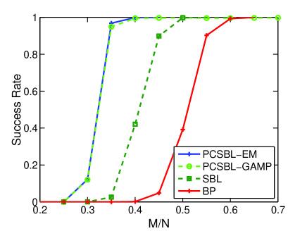
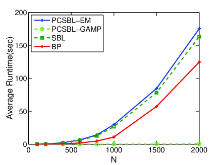
We first evaluate the recovery performance of the PCSBL-GAMP method using the synthetic data. In our simulations, we generate a one-dimensional block-sparse signal in a way similar to [21]. Suppose the $N$-dimensional sparse signal contains $K$ nonzero coefficients ($K$ is also denoted as the sparsity level) which are partitioned into $T$ blocks with random sizes and random locations. The nonzero coefficients of the sparse signal $\boldsymbol{x}$ and the measurement matrix $\boldsymbol{A}\in\mathbb{R}^{M\times N}$ are randomly generated with each entry independently drawn from a normal distribution, and then the sparse signal $\boldsymbol{x}$ and columns of $\boldsymbol{A}$ are normalized to unit norm. Fig. 1 depicts the success rate of the proposed PCSBL-GAMP method vs. the ratio $M/N$, where we set $N=200$, $K=40$ and $T=6$. The success rate is computed as the ratio of the number of successful trials to the total number of independent runs. A trial is considered successful if the normalized squared recovery error $\|\boldsymbol{x}-\boldsymbol{\hat{x}}\|^{2}/\|\boldsymbol{x}\|^{2}$ is no greater than $10^{-6}$, where $\boldsymbol{\hat{x}}$ denotes the estimate of the sparse signal. The success rates of the EM-based PC-SBL method [21] (referred to as the PCSBL-EM), the conventional SBL [4], and the basis pursuit (BP) method [2, 24] are also included for comparison. From Fig. 1, we see that the PCSBL-GAMP method achieves almost the same performance as that of the PCSBL-EM method, and presents a significant performance advantage over the SBL and BP methods due to exploiting the underlying block-sparse structures. The average run times of respective algorithms as a function of the signal dimension $N$ is plotted in Fig. 2, where we set $M=0.4N$. Results are averaged over 100 independent runs. We see that the PCSBL-GAMP requires much less run time than the PCSBL-EM, particularly when the signal dimension $N$ is large. Also, it can be observed that the average run time of the PCSBL-EM grows rapidly with an increasing $N$, whereas the average run time of the PCSBL-GAMP increases very slowly. This observation coincides with our computational complexity analysis.

Figure 1: Success rates vs. the ratio $M/N$.

Figure 2: Average run times vs. $N$.

Figure 3: Original patches of letters and patches reconstructed by respective algorithms.

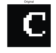
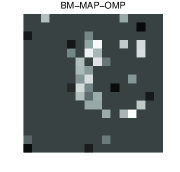
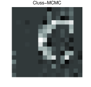
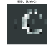
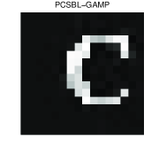
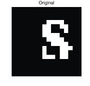
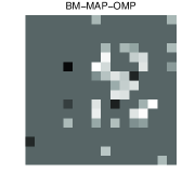
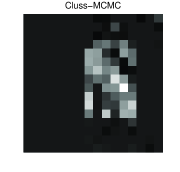
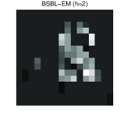
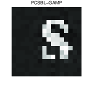
We also carry out experiments using patches of letters “C” and “S” ($16\times 16$ pixels) with black background, where most of the pixels on the patches are zeros and the nonzero coefficients exhibit irregular block patterns. White Gaussian noise is added to the patches. We compare our method with other block-sparse signal recovery algorithms, namely, the cluster-structured MCMC algorithm (Cluss-MCMC) [17], the Boltzman machine-based greedy pursuit algorithm (BM-MAP-OMP) [18], and the block sparse Bayesian learning method (BSBL) method [15, 20]. Note that although the BM-MAP-OMP and the BSBL algorithms are developed for one-dimensional sparse signal recovery, we extend their methods to the two-dimensional scenario. In our simulations, model parameters used by the competing algorithms are adjusted to achieve the best performance. For the BSBL algorithms, the block size parameter $h$ is set equal to 2. Fig. 3 depicts the original patches and the patches reconstructed by respective algorithms, where we set $M=80$, and the signal-to-noise ratio (SNR) is set to 20dB with $\text{SNR}\triangleq 10\log(\|\boldsymbol{Ax}\|_{2}^{2}/M\sigma^{2})$. It can be seen that our proposed PCSBL-GAMP method provides the best visual quality with recognizable letters, whereas the letters reconstructed by other algorithms have considerably lower quality, particularly for the Cluss-MCMC and the BM-MAP-OMP methods. This result also implies that our proposed method is flexible to accommodate any irregular cluster patterns.

Figure 4: Original satellite image and images reconstructed by respective algorithms.

IV-B Satellite Image Recovery

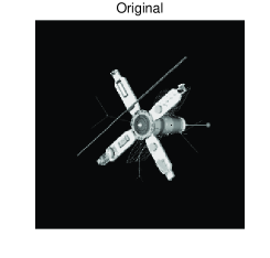
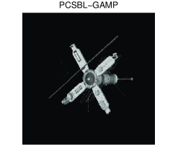
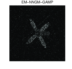
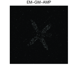
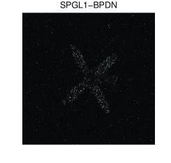
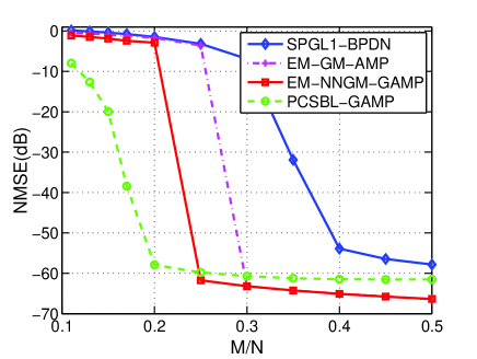
In this subsection, we carry out experiments on a non-negative $256\times 256$ satellite image. The image is sparse in the spatial domain, with only $6678$ (approximately $10.2\%$ of total pixels) nonzero pixels. In our experiments, compressive measurements are corrupted by additive i.i.d. Gaussian noise, i.e. $\boldsymbol{y}=\boldsymbol{Ax}+\boldsymbol{w}$, where the image is represented as a one-dimensional vector $\boldsymbol{x}$. The sensing matrix $\boldsymbol{A}$ is chosen to be the same as that used in [25], i.e. $\boldsymbol{A}=\boldsymbol{\Phi\Psi S}$, where $\boldsymbol{\Phi}\in\{0,1\}^{M\times N}$ and its rows are randomly selected from the $N\times N$ identity matrix, $\boldsymbol{\Psi}\in\{-1,1\}^{N\times N}$ is a Hadamard transform matrix, $\boldsymbol{S}\in\mathbb{R}^{N\times N}$ is a diagonal matrix with its entries randomly chosen from $\{-1,1\}$. Sensing using such a measurement matrix can be executed using a fast binary algorithm, which makes the hardware implementation simple. Note that the BM-MAP-OMP, the BSBL and the Cluss-MCMC methods were not included in this experiment due to their prohibitive computational complexity when the signal dimension is large. Instead, we compare our method with some other computationally efficient GAMP-based methods, namely, the EM-NNGM-GAMP method [25] and the EM-GM-AMP method [26]. These two methods have demonstrated state-of-the-art recovery performance in a series of experiments. The spectral projected gradient (SPG) method (referred to as SPGL1) which was developed in [27] to efficiently solve the basis pursuit or basis pursuit denoising optimizations is also included for comparison. Among these methods, only the EM-NNGM-GAMP algorithm exploits the non-negativity of the satellite image. Therefore the signals recovered by these algorithms, except the EM-NNGM-GAMP, may contain negative coefficients. These negative coefficients are manually set to zero in our simulations. Fig. 4 shows the original satellite image and the images reconstructed by respective algorithms, where we set $M=0.15N$ and $\text{SNR}=60\text{dB}$. It can be seen that the PCSBL-GAMP offers a significantly better image quality as compared with other methods. Fig. 5 plots the normalized mean square errors (NMSEs) of respective algorithms vs. the ratio $M/N$. Results are averaged over 100 independent trails, with the sensing matrix $\boldsymbol{A}$ randomly generated for each trial. The recovered negative coefficients are kept unaltered in calculating the NMSEs. We see that our proposed PCSBL-GAMP method outperforms other algorithms by a big margin for a small ratio $M/N$ (e.g. $M/N\leq 0.25$), where data acquisition is practically appealing due to high compression rates.

Figure 5: Satellite image: NMSEs vs. the ratio $M/N$.

IV-C Background Subtraction

Background subtraction, also known as foreground detection, is a technique used to automatically detect and track moving objects in videos from static cameras. Usually, the foreground innovations are sparse in the spatial image domain. By exploiting this sparsity, the sparse foreground innovations within a scene can be reconstructed using compressed measurements, which relieves the communications burden placed on data transmission [8]. Specifically, the idea is to reconstruct the foreground image from the difference between the compressed measurements of the background image and the compressed measurements of the test image [8]

$$\boldsymbol{y}_{f}= \boldsymbol{y}_{t}-\boldsymbol{y}_{b}=\boldsymbol{A}(\boldsymbol{x}_{t}-\boldsymbol{x}_{b})$$

$$= \boldsymbol{A}\boldsymbol{x}_{f}$$

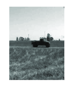
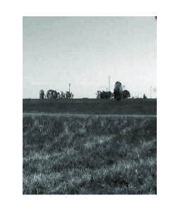
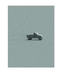
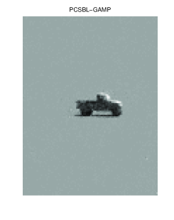
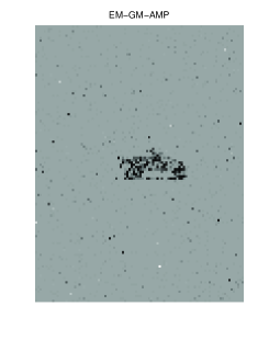
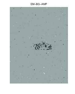
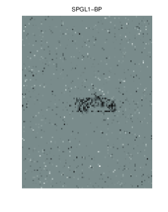
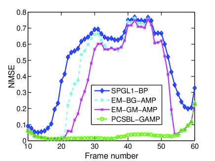
where $\boldsymbol{x}_{t}$ and $\boldsymbol{x}_{b}$ represent the test and the background images, respectively; $\boldsymbol{y}_{t}$ and $\boldsymbol{y}_{b}$ denote the compressed measurements of the test and background images, respectively; and $\boldsymbol{x}_{f}$ is the foreground image to be recovered. In our experiments, we use the Convoy2 data set that was used in [28]. The Convoy2 data set was collected on the Spesutie island, consisting of a video sequence with $260$ frames and one background frame recorded by a single static camera. The video sequence has a dynamic sparse foreground as vehicles enter and exit the filed of view over time. We first choose the $40$th frame of the Convoy2 data set as a test image, which is shown in Fig. 6. The background image and the foreground image are also included in Fig. 6. The foreground image is regarded as the groundtruth image. This foreground image, however, does not have a pure background since $\boldsymbol{x}_{f}=\boldsymbol{x}_{t}-\boldsymbol{x}_{b}$ is not an exactly sparse signal and contains many small nonzero components. In our experiments, the original images of $480\times 381$ pixels are resized to $120\times 96$ pixels. For the resized foreground image, we have a total number of $923$ coefficients whose magnitudes are greater than $10^{-2}$, thus the percentage of nonzero coefficients is $923/(120\times 96)=8.01\%$. Again, the BM-MAP-OMP, BSBL, and the Cluss-MCMC methods are not included due to their prohibitive computational complexity. Here we compare our method with the EM-GM-AMP method [26] and the EM-BG-AMP method [29]. Fig. 7 depicts images reconstructed by respective algorithms, where we use only $M=0.1N$ measurements. The measurement matrix $\boldsymbol{A}$ is randomly generated with each entry independently drawn from a normal distribution. We see that our proposed PCSBL-GAMP method provides the finest image quality with a clear appearance of the vehicle, whereas the object silhouettes recovered by other methods are hardly recognizable. In our next experiments, frames from the 10th to 60th are used as test images. For each test image, we use $M=0.1N$ measurements to recover the difference (foreground) image. Fig. 8 shows the NMSEs of respective algorithms vs. the frame number, where the NMSEs are obtained by averaging over 100 independent runs, with the measurement matrix $\boldsymbol{A}$ randomly generated for each run. From Fig. 8, we observe that our proposed method presents a significant performance advantage over other methods.

Figure 6: From left to right: the test image $\boldsymbol{x}_{t}$ (40th frame of the Convoy2 data set), the background image $\boldsymbol{x}_{b}$, the foreground image $\boldsymbol{x}_{f}$.

Figure 7: Foreground images reconstructed by respective algorithms.

V Conclusions

We developed a pattern-coupled sparse Bayesian learning method for recovery of two-dimensional block-sparse signals whose cluster patterns are unknown a priori. A two-dimensional pattern-coupled hierarchical Gaussian prior model is introduced to characterize and exploit the pattern dependencies among neighboring coefficients. The proposed pattern-coupled hierarchical model is effective and flexible to capture any underlying block-sparse structures, without requiring the prior knowledge of the block partition. An expectation-maximization (EM) strategy is employed to infer the maximum a posterior (MAP) estimate of the hyperparameters, along with the posterior distribution of the sparse signal. Additionally, the generalized approximate message passing (GAMP) algorithm is embedded in the EM framework to efficiently compute an approximation of the posterior distribution of hidden variables, which results in a significant reduction in computational complexity. Numerical results show that our proposed algorithm presents a substantial performance advantage over other existing state-of-the-art methods in image recovery.

Figure 8: NMSEs vs. the frame number.

References

- [1] J. A. Tropp and A. C. Gilbert, “Signal recovery from random measurements via orthogonal matching pursuit,” IEEE Trans. Information Theory, vol. 53, no. 12, pp. 4655–4666, Dec. 2007.
- [2] S. S. Chen, D. L. Donoho, and M. A. Saunders, “Atomic decomposition by basis pursuit,” SIAM J. Sci. Comput., vol. 20, no. 1, pp. 33–61, 1998.
- [3] D. Wipf and S. Nagarajan, “Iterative reweighted and methods for finding sparse solutions,” IEEE Journals of Selected Topics in Signal Processing, vol. 4, no. 2, pp. 317–329, Apr. 2010.
- [4] M. Tipping, “Sparse Bayesian learning and the relevance vector machine,” Journal of Machine Learning Research, vol. 1, pp. 211–244, 2001.
- [5] S. Ji, Y. Xue, and L. Carin, “Bayesian compressive sensing,” IEEE Trans. Signal Processing, vol. 56, no. 6, pp. 2346–2356, June 2008.
- [6] Z. Yang, L. Xie, and C. Zhang, “Off-grid direction of arrival estimation using sparse Bayesian inference,” IEEE Trans. Signal Processing, vol. 61, no. 1, pp. 38–42, Jan. 2013.
- [7] L. Wang, L. Zhao, G. Bi, C. Wan, and L. Yang, “Enhanced ISAR imaging by exploiting the continuity of the target scene,” IEEE Trans. Geoscience and Remote Sensing, no. 9, pp. 5736–5750, Sept. 2014.
- [8] V. Cevher, A. Sankaranarayanan, M. F. Duarte, D. Reddy, R. G. Baraniuk, and R. Chellappa, “Compressive sensing for background subtraction,” in European Conf. Comp. Vision (ECCV), Marseille, France, October 12-18 2008.
- [9] N. Vaswani and W. Lu, “Modified-CS: modifying compressive sensing for problems with partially known support,” IEEE Trans. Signal Processing, no. 9, pp. 4595–4607, September 2010.
- [10] Y. C. Eldar and M. Mishali, “Robust recovery of signals from a structured union of subspaces,” IEEE Trans. Information Theory, vol. 55, no. 11, pp. 5302–5316, Nov. 2009.
- [11] R. G. Baraniuk, V. Cevher, M. F. Duarte, and C. Hegde, “Model-based compressive sensing,” IEEE Trans. Information Theoy, vol. 56, no. 4, pp. 1982–2001, Apr. 2010.
- [12] Y. C. Eldar, P. Kuppinger, and H. Bölcskei, “Block-sparse signals: uncertainty relations and efficient recovery,” IEEE Trans. Information Theory, vol. 58, no. 6, pp. 3042–3054, June 2010.
- [13] M. Yuan and Y. Lin, “Model selection and estimation in regression with grouped variables,” J. R. Statist. Soc. B, vol. 68, pp. 49–67, 2006.
- [14] D. P. Wipf and B. D. Rao, “An empirical Bayesian strategy for solving the simultaneous sparse approximation problem,” IEEE Trans. Signal Processing, vol. 55, no. 7, pp. 3704–3716, July 2007.
- [15] Z. Zhang and B. D. Rao, “Sparse signal recovery with temporally correlated source vectors using sparse Bayesian learning,” IEEE Journal of Selected Topics in Signal Processing, vol. 5, no. 5, pp. 912–926, Sept. 2011.
- [16] L. He and L. Carin, “Exploiting structure in wavelet-based Bayesian compressive sensing,” IEEE Trans. Signal Processing, vol. 57, no. 9, pp. 3488–3497, Sept. 2009.
- [17] L. Yu, H. Sun, J. P. Barbot, and G. Zheng, “Bayesian compressive sensing for cluster structured sparse signals,” Signal Processing, vol. 92, pp. 259–269, 2012.
- [18] T. Peleg, Y. C. Eldar, and M. Elad, “Exploiting statistical dependencies in sparse representations for signal recovery,” IEEE Trans. Signal Processing, vol. 60, no. 5, pp. 2286–2303, May 2012.
- [19] A. Drámeau, C. Herzet, and L. Daudet, “Boltzmann machine and mean-field approximation for structured sparse decompositions,” IEEE Trans. Signal Processing, vol. 60, no. 7, pp. 3425–3438, July 2012.
- [20] Z. Zhang and B. D. Rao, “Extension of SBL algorithms for the recovery of block sparse signals with intra-block correlation,” IEEE Trans. Signal Processing, vol. 61, no. 8, pp. 2009–2015, Apr. 2013.
- [21] J. Fang, Y. Shen, H. Li, and P. Wang, “Pattern-coupled sparse Bayesian learning for recovery of block-sparse signals,” IEEE Trans. Signal Processing, no. 2, pp. 360–372, Jan. 2015.
- [22] S. Rangan, “Generalized approximate message passing for estimation with random linear mixing,” in Proc. IEEE Int. Symp. Inf. Theory (ISIT), Saint Petersburg, Russia, Aug. 2011.
- [23] D. L. Donoho, A. Maleki, and A. Montanari, “Message passing algorithms for compressed sensing: I. motivation and construction,” in Proc. Inf. Theory Workshop, Cairo, Egypt, Jan. 2010.
- [24] E. Candés and T. Tao, “Decoding by linear programming,” IEEE Trans. Information Theory, no. 12, pp. 4203–4215, Dec. 2005.
- [25] J. P. Vila and P. Schniter, “An empiricla-Bayes approach to recovering linearly constrained non-negative sparse signals,” IEEE Trans. Signal Processing, vol. 62, no. 18, pp. 4689–4703, Sep 2014.
- [26] ——, “Expectation-maximization Gaussian-mixture approximate message passing,” IEEE Trans. Signal Processing, no. 19, pp. 4658–4672, Oct. 2013.
- [27] E. van den Berg and M. P. Friedlander, “Probing the Pareto frontier for basis pursuit solutions,” SIAM J. Sci. Comput, vol. 31, no. 2, pp. 890–912, 2008.
- [28] G. Warnell, D. Reddy, and R. Chellappa, “Adaptive rate compressive sensing for background subtraction,” in IEEE International Conference on Acoustics, Speech and Signal Processing (ICASSP), Kyoto, Japan, March 25-30 2012.
- [29] J. P. Vila and P. Schniter, “Expectation-maximization Bernoulli-Gaussian approximate message passing,” in 45th Asilomar Conference on Signals, Symtems and computers, Pacific Grove, CA, USA, November 6-9 2011.