On a linear non-homogeneous ordinary differential equation of the higher order whose coefficients are real-valued simple step functions

Abstract

By using the method developed in the paper [G.Pantsulaia, G.Giorgadze, On some applications of infinite-dimensional cellular matrices, Georg. Inter. J. Sci. Tech., Nova Science Publishers, Volume 3, Issue 1 (2011), 107-129], it is obtained a representation in an explicit form of the particular solution of the linear non-homogeneous ordinary differential equation of the higher order whose coefficients are real-valued simple functions.

2000 Mathematics Subject Classification: Primary 34Axx ; Secondary 34A35, 34K06.

Key words and phrases: linear ordinary differential equation, non-homogeneous ordinary differential equation.

1. Introduction

In [4] has been obtained a representation in an explicit form of the particular solution of the linear non-homogeneous ordinary differential equation of the higher order with real-valued coefficients. The aim of the present manuscript is resolve an analogous problem for a linear non-homogeneous ordinary differential equation of the higher order when coefficients are real-valued simple step functions.

The paper is organized as follows.

In Section 2, we consider some auxiliary results obtained in the paper [4]. In Section 3, it is obtained a representation in an explicit form of the particular solution of the linear non-homogeneous ordinary differential equation of the higher order whose coefficients are real-valued simple functions. In Section 4 we present mathematical programm in MathLab for the graphical solution of the corresponding differential equation.

2. Some auxiliary propositions

For $n\in N$, we denote by $FD^{(n)}[-l,l[$ a vector space of all $n$-times differentiable functions $\Psi$ on $[-l,l[$ such that a series obtained by $k$-times differentiation term by term of the Fourier trigonometric series of $\Psi$ pointwise converges to $\Psi^{(k)}$ for all $x\in[-l,l[$ and $0\leq k\leq n$.

Let $(A_{n})_{0\leq n\leq 2M}$ be a sequence of real numbers, where $M$ is any natural number. For each $k\geq 1$ we put

$$\sigma_{k}=\sum_{n=0}^{m}(-1)^{n}A_{2n}(\frac{k\pi}{l})^{2n},$$

$$\omega_{k}=\sum_{n=0}^{m-1}(-1)^{n}A_{2n+1}(\frac{k\pi}{l})^{2n+1}.$$

Theorem 2.1.

([4], Theorem 3.1, p.45) For $m\geq 1$, let us consider an ordinary differential equation

$$\sum_{n=0}^{2m}A_{n}\frac{d^{n}}{dx^{n}}\Psi=f,$$

where

$$f(x)=\frac{c_{0}}{2}+\sum_{k=1}^{\infty}c_{k}\cos\Big{(}\frac{k\pi x}{l}\Big{)}+d_{k}\sin\Big{(}\frac{k\pi x}{l}\Big{)}\in FD^{(0)}[-l,l[$$

and $A_{n}\in R$ for $0\leq n\leq 2m$.

Suppose that $A_{0}\neq 0$ and $\sigma_{k}^{2}+\omega_{k}^{2}\neq 0$ for $k\geq 1$, where $\sigma_{k}$ and $\omega_{k}$ are defined by (2.1) and (2.2), respectively.

If $(\frac{c_{0}}{2},c_{1},d_{1},c_{2},d_{2},\dots)$ is such a sequence of real numbers that the series $\Psi_{p}$, defined by

$$\Psi_{p}(x)=\frac{c_{0}}{2A_{0}}+\sum_{k=1}^{\infty}\Big{(}\frac{c_{k}\sigma_{k}-d_{k}\omega_{k}}{\sigma_{k}^{2}+\omega_{k}^{2}}\Big{)}\cos\Big{(}\frac{k\pi x}{l}\Big{)}+\Big{(}\frac{c_{k}\omega_{k}+d_{k}\sigma_{k}}{\sigma_{k}^{2}+\omega_{k}^{2}}\Big{)}\sin\Big{(}\frac{k\pi x}{l}\Big{)},$$

belongs to the class $FD^{(2m)}[-l,l[$, then $\Psi_{p}$ is a particular solution of (2.3).

Theorem 2.2.

([4], Theorem 3.2, p.45) For $m\geq 1$, let us consider an ordinary differential equation (2.3), where

$$f(x)\in C[-l,l]$$

and $A_{n}\in R$ for $0\leq n\leq 2m$.

Suppose that $A_{0}\neq 0$ and $\sigma_{k}^{2}+\omega_{k}^{2}\neq 0$ for $k\geq 1$, where $\sigma_{k}$ and $\omega_{k}$ are defined by (2.1) and (2.2), respectively. Let $(\frac{c_{0}}{2},c_{1},d_{1},c_{2},d_{2},\dots)$ be Fourier coefficients of $f$ and $(\frac{c_{0}}{2},c_{1},d_{1},c_{2},d_{2},\dots)\in\ell_{1}.$

Then the series $\Psi_{p}$, defined by

$$\Psi_{p}(x)=\frac{c_{0}}{2A_{0}}+\sum_{k=1}^{\infty}\Big{(}\frac{c_{k}\sigma_{k}-d_{k}\omega_{k}}{\sigma_{k}^{2}+\omega_{k}^{2}}\Big{)}\cos\Big{(}\frac{k\pi x}{l}\Big{)}+\Big{(}\frac{c_{k}\omega_{k}+d_{k}\sigma_{k}}{\sigma_{k}^{2}+\omega_{k}^{2}}\Big{)}\sin\Big{(}\frac{k\pi x}{l}\Big{)},$$

is a particular solution of (2.3).

3. A non-homogeneous ordinary differential equation of higher order whose coefficients are continuous or real-valued step functions

Let consider a partition of $[-l,l[$ defined by

$$[-l,l[=\cup_{s=0}^{S-1}[\frac{l(2s-S)}{S},\frac{l(2s+2-S)}{S}[)$$

We define a differential operator

$$L(\Psi)=\sum_{n=0}^{2m}A_{n}(x)\frac{d^{n}}{dx^{n}}\Psi$$

for $\Psi\in FD^{(2m)}[-l,l[$. Notice that $L(\Psi)$ can be rewritten as follows

$$L(\Psi)=\cup_{s=0}^{S-1}Ind_{[\frac{l(2s-S)}{S},\frac{l(2s+2-S)}{S}[}\big{(}\sum_{n=0}^{2m}A_{n}(x)\frac{d^{n}}{dx^{n}}\big{)}\Psi$$

for $\Psi\in FD^{(2m)}[-l,l[$, where $Ind$ denotes an indicator function.

For each $S\in\mathbb{N}$ we define an operator $L_{S}$ by

$$L_{S}(\Psi)=\sum_{s=0}^{S-1}Ind_{[\frac{l(2s-S)}{S},\frac{l(2s+2-S)}{S}[}\big{(}\sum_{n=0}^{2m}A_{n}(\frac{l(2s+1-S)}{S})\frac{d^{n}}{dx^{n}}\big{)}\Psi$$

for $\Psi\in FD^{(2m)}[-l,l]$.

Lemma 3.1.

For each $\Psi\in FD^{(2m)}[-l,l[$ we have

$$L(\Psi)=\lim_{S\to\infty}L_{S}(\Psi).$$

Theorem 3.2.

For $m\geq 1$, let us consider an ordinary differential equation

$$\sum_{n=0}^{2m}A_{n}(x)\frac{d^{n}}{dx^{n}}\Psi=f,$$

where

$$f(x)=\frac{c_{0}}{2}+\sum_{k=1}^{\infty}c_{k}\cos\Big{(}\frac{k\pi x}{l}\Big{)}+d_{k}\sin\Big{(}\frac{k\pi x}{l}\Big{)}\in FD^{(0)}[-l,l[$$

and $A_{n}(x)\in C[-l,l]$ for $0\leq n\leq 2m$.

Suppose that $A_{0}(x)=1$ and $\sigma_{k}^{2}(x)+\omega_{k}^{2}(x)\neq 0$ for $x\in[-l,l[$ and $k\geq 1$, where $\sigma_{k}(x)$ and $\omega_{k}(x)$ are defined by

$$\sigma_{k}(x)=\sum_{n=0}^{m}(-1)^{n}A_{2n}(x)(\frac{k\pi}{l})^{2n},$$

$$\omega_{k}(x)=\sum_{n=0}^{m-1}(-1)^{n}A_{2n+1}(x)(\frac{k\pi}{l})^{2n+1}.$$

Suppose that the following conditions are valid:

(i) $(\frac{c_{0}}{2},c_{1},d_{1},c_{2},d_{2},\dots)\in\ell_{1}$;

(iii) There is a constant $C>0$ such that

$$\Big{|}\frac{\omega_{k}(x+h)}{\sigma_{k}^{2}(x+h)+\omega_{k}^{2}(x+h)}-\frac{\omega_{k}(x)}{\sigma_{k}^{2}(x)+\omega_{k}^{2}(x)}\Big{|}\leq C|h|^{2}$$

and

$$\Big{|}\frac{\sigma_{k}(x+h)}{\sigma_{k}^{2}(x+h)+\omega_{k}^{2}(x+h)}-\frac{\sigma_{k}(x)}{\sigma_{k}^{2}(x)+\omega_{k}^{2}(x)}\Big{|}\leq C|h|^{2}.$$

Then the function $\Psi_{0}$, defined by

$$\Psi_{0}(x)=\frac{c_{0}}{2}+\sum_{k=1}^{\infty}\Big{(}\frac{c_{k}\sigma_{k}(x)-d_{k}\omega_{k}(x)}{\sigma_{k}^{2}(x)+\omega_{k}^{2}(x)}\Big{)}\cos\Big{(}\frac{k\pi x}{l}\Big{)}+$$

$$\Big{(}\frac{c_{k}\omega_{k}(x)+d_{k}\sigma_{k}(x)}{\sigma_{k}^{2}(x)+\omega_{k}^{2}(x)}\Big{)}\sin\Big{(}\frac{k\pi x}{l}\Big{)},$$

is a particular solution of (3.1).

Proof.

We put

$$\Psi_{S}(x)=\sum_{s=0}^{S-1}Ind_{[\frac{l(2s-S)}{S},\frac{l(2s+2-S)}{S}[}(x)\Big{[}\frac{c_{0}}{2}+$$

$$\sum_{k=1}^{\infty}\Big{(}\frac{c_{k}\sigma_{k}(\frac{l(2s+1-S)}{S})-d_{k}\omega_{k}(\frac{l(2s+1-S)}{S})}{\sigma_{k}^{2}(\frac{l(2s+1-S)}{S})+\omega_{k}^{2}(\frac{l(2s+1-S)}{S})}\Big{)}\cos\Big{(}\frac{k\pi x}{l}\Big{)}+$$

$$\Big{(}\frac{c_{k}\omega_{k}(\frac{l(2s+1-S)}{S})+d_{k}\sigma_{k}(\frac{l(2s+1-S)}{S})}{\sigma_{k}^{2}(\frac{l(2s+1-S)}{S})+\omega_{k}^{2}(\frac{l(2s+1-S)}{S})}\Big{)}\sin\Big{(}\frac{k\pi x}{l}\Big{)}\Big{]},$$

On the one hand, by using the result of Lemma 3.1 we have

$$L(\lim_{S\to\infty}\Psi_{S}(x))=\lim_{S\to\infty}L(\Psi_{S}(x))=\lim_{S\to\infty}L_{S}(\Psi_{S}(x))=\lim_{S\to\infty}f(x)=f(x).$$

On the other hand we have

$$|\lim_{S\to\infty}\Psi_{S}(x)-\Psi_{0}(x))|=\lim_{S\to\infty}|\Psi_{S}(x)-\Psi_{0}(x)|=\lim_{S\to\infty}\Big{|}\sum_{s=0}^{S-1}Ind_{[\frac{l(2s-S)}{S},\frac{l(2s+2-S)}{S}[}(x)\Big{[}\Big{(}\frac{c_{0}}{2}-\frac{c_{0}}{2}\Big{)}+$$

$$\sum_{k=1}^{\infty}\Big{(}\frac{c_{k}\sigma_{k}(\frac{l(2s+1-S)}{S})-d_{k}\omega_{k}(\frac{l(2s+1-S)}{S})}{\sigma_{k}^{2}(\frac{l(2s+1-S)}{S})+\omega_{k}^{2}(\frac{l(2s+1-S)}{S})}-\frac{c_{k}\sigma_{k}(x)-d_{k}\omega_{k}(x)}{\sigma_{k}^{2}(x)+\omega_{k}^{2}(x)}\Big{)}\cos\Big{(}\frac{k\pi x}{l}\Big{)}+$$

$$\Big{(}\frac{c_{k}\omega_{k}(\frac{l(2s+1-S)}{S})+d_{k}\sigma_{k}(\frac{l(2s+1-S)}{S})}{\sigma_{k}^{2}(\frac{l(2s+1-S)}{S})+\omega_{k}^{2}(\frac{l(2s+1-S)}{S})}-\frac{c_{k}\omega_{k}(x)+d_{k}\sigma_{k}(x)}{\sigma_{k}^{2}(x)+\omega_{k}^{2}(x)}\Big{)}\sin\Big{(}\frac{k\pi x}{l}\Big{)}\Big{]}\Big{|}\leq$$

$$\lim_{S\to\infty}\sum_{s=0}^{S-1}\sup_{x\in[\frac{l(2s-S)}{S},\frac{l(2s+2-S)}{S}[}\{\sum_{k=1}^{\infty}\Big{|}\frac{c_{k}\sigma_{k}(\frac{l(2s+1-S)}{S})-d_{k}\omega_{k}(\frac{l(2s+1-S)}{S})}{\sigma_{k}^{2}(\frac{l(2s+1-S)}{S})+\omega_{k}^{2}(\frac{l(2s+1-S)}{S})}-\frac{c_{k}\sigma_{k}(x)-d_{k}\omega_{k}(x)}{\sigma_{k}^{2}(x)+\omega_{k}^{2}(x)}\Big{|}+$$

$$\Big{|}\frac{c_{k}\omega_{k}(\frac{l(2s+1-S)}{S})+d_{k}\sigma_{k}(\frac{l(2s+1-S)}{S})}{\sigma_{k}^{2}(\frac{l(2s+1-S)}{S})+\omega_{k}^{2}(\frac{l(2s+1-S)}{S})}-\frac{c_{k}\omega_{k}(x)+d_{k}\sigma_{k}(x)}{\sigma_{k}^{2}(x)+\omega_{k}^{2}(x)}\Big{|}\}=$$

$$\lim_{S\to\infty}\sum_{s=0}^{S-1}\sup_{x\in[\frac{l(2s-S)}{S},\frac{l(2s+2-S)}{S}[}\{\sum_{k=1}^{\infty}\Big{|}c_{k}(\frac{\sigma_{k}(\frac{l(2s+1-S)}{S})}{\sigma_{k}^{2}(\frac{l(2s+1-S)}{S})+\omega_{k}^{2}(\frac{l(2s+1-S)}{S})}-\frac{\sigma_{k}(x)}{\sigma_{k}^{2}(x)+\omega_{k}^{2}(x)})-$$

$$d_{k}(\frac{\omega_{k}(\frac{l(2s+1-S)}{S}))}{\sigma_{k}^{2}(\frac{l(2s+1-S)}{S})+\omega_{k}^{2}(\frac{l(2s+1-S)}{S})}-\frac{\omega_{k}(x)}{\sigma_{k}^{2}(x)+\omega_{k}^{2}(x)})\Big{|}+$$

$$\Big{|}d_{k}(\frac{\sigma_{k}(\frac{l(2s+1-S)}{S})}{\sigma_{k}^{2}(\frac{l(2s+1-S)}{S})+\omega_{k}^{2}(\frac{l(2s+1-S)}{S})}-\frac{\sigma_{k}(x)}{\sigma_{k}^{2}(x)+\omega_{k}^{2}(x)})+$$

$$c_{k}(\frac{\omega_{k}(\frac{l(2s+1-S)}{S}))}{\sigma_{k}^{2}(\frac{l(2s+1-S)}{S})+\omega_{k}^{2}(\frac{l(2s+1-S)}{S})}-\frac{\omega_{k}(x)}{\sigma_{k}^{2}(x)+\omega_{k}^{2}(x)})\Big{|}\}\leq$$

$$\lim_{S\to\infty}\sum_{s=0}^{S-1}\sup_{x\in[\frac{l(2s-S)}{S},\frac{l(2s+2-S)}{S}[}\{\sum_{k=1}^{\infty}2(|c_{k}|+|d_{k}|)\frac{4l^{2}C}{S^{2}}\}\leq$$

$$\lim_{S\to\infty}\frac{8l^{2}C}{S}\sum_{k=1}^{\infty}(|c_{k}|+|d_{k}|)=0.$$

∎

Remark 3.3.

Theorem 3.2 is a generalization of Theorem 2.2. Indeed, Theorem 2.2 is a simple consequence of Theorem 3.2, when $A_{n}(x)=const$ for $0\leq n\leq 2m$, because in that cases all conditions of Theorem 3.2 are fulfilled.

We say that $(a_{k})_{0\leq k\leq s}$ is partition of $[-l,l[$ if $-l=a_{0}<a_{1}<\cdots<a_{s-1}<a_{s}=l$.

We say that a real-valued function $f$ on $[-l,l[$ is simple function if there exists a partition $(a_{k})_{0\leq k\leq s}$ of $[-l,l[$ and a sequence of real numbers $(A_{k})_{1\leq k\leq s}$ such that

$$f(x)=\sum_{k=1}^{s}A_{k}Ind_{[a_{k-1},a_{k})}(x)$$

for $x\in[-l,l[$.

We have the following proposition.

Theorem 3.4.

Suppose that $(A_{n}(x))_{0\leq n\leq 2m}$ is a sequence of real-valued simple step functions on $[-l,l[$, i.e. for every $n~{}(0\leq n\leq 2m)$ there exists a partition $(a^{(n)}_{k})_{0\leq k\leq s_{n}}$ of $[-l,l[$ and a sequence of real numbers $(A^{(n)}_{k})_{1\leq k\leq s_{n}}$ such that

$$A_{n}(x)=\sum_{k=1}^{s_{n}}A^{(n)}_{k}Ind_{[a^{(n)}_{k-1},a^{(n)}_{k})}(x)$$

for $x\in[-l,l[$.

Suppose that $A_{0}(x)$ does not remain a zero value on $[-l,l[$ and $\sigma_{k}^{2}(x)+\omega_{k}^{2}(x)\neq 0$ for $x\in[-l,l[$ and $k\geq 1$, where $\sigma_{k}(x)$ and $\omega_{k}(x)$ are defined by (3.3) and (3.4). Suppose also that Fourier coefficients of the function $f$ standing in the right side of the equation (3.1) satisfy the following condition $(\frac{c_{0}}{2},c_{1},d_{1},c_{2},d_{2},\dots)\in\ell_{1}$.

Then the function $\Psi_{0}$, defined by

$$\Psi_{0}(x)=\frac{c_{0}}{2A_{0}(x)}+\sum_{k=1}^{\infty}\Big{(}\frac{c_{k}\sigma_{k}(x)-d_{k}\omega_{k}(x)}{\sigma_{k}^{2}(x)+\omega_{k}^{2}(x)}\Big{)}\cos\Big{(}\frac{k\pi x}{l}\Big{)}+$$

$$\Big{(}\frac{c_{k}\omega_{k}(x)+d_{k}\sigma_{k}(x)}{\sigma_{k}^{2}(x)+\omega_{k}^{2}(x)}\Big{)}\sin\Big{(}\frac{k\pi x}{l}\Big{)},$$

for $x\in[-l,l[$, satisfies (3.1)–(3.2) at each point of the set

$$(-l,l)\setminus\cup_{0\leq n\leq 2m}\{a^{(n)}_{1},a^{(n)}_{2},\cdots,a^{(n)}_{s_{n}-1}\}$$

.

Proof.

If $x_{0}\in(-l,l)\setminus G(:=\cup_{0\leq n\leq 2m}\{a^{(n)}_{1},a^{(n)}_{2},\cdots,a^{(n)}_{s_{n}-1}\})$, then by virtue of the openness of the $G$ there exists a positive real number $r>0$ such that $(x_{0}-r,x_{0}+r)\subseteq G$. It is obvious that $(A_{n}(x)$ is constant on $(x_{0}-r,x_{0}+r)$ for $0\leq n\leq 2m$. We set $A_{n}:=A_{n}(x_{0})$ for $0\leq n\leq 2m$.

For $m\geq 1$, let us consider an ordinary differential equation

$$\sum_{n=0}^{2m}A_{n}\frac{d^{n}}{dx^{n}}\Psi=f.$$

Note that for (3.8) all conditions of Theorem 2.2 are fulfilled. Hence the series $\Psi_{p}$, defined by

$$\Psi_{p}(x)=\frac{c_{0}}{2A_{0}}+\sum_{k=1}^{\infty}\Big{(}\frac{c_{k}\sigma_{k}-d_{k}\omega_{k}}{\sigma_{k}^{2}+\omega_{k}^{2}}\Big{)}\cos\Big{(}\frac{k\pi x}{l}\Big{)}+$$

$$\Big{(}\frac{c_{k}\omega_{k}+d_{k}\sigma_{k}}{\sigma_{k}^{2}+\omega_{k}^{2}}\Big{)}\sin\Big{(}\frac{k\pi x}{l}\Big{)},$$

is a particular solution of (3.8), where $\sigma_{k}$ and $\omega_{k}$ are defined by (2.1) and (2.2), respectively.

Notice that $\Psi_{p}$ defined by (3.9) coincides with $\psi_{0}$ defined by (3.7) at all point $x\in(x_{0}-r,x_{0}+r)$. Similarly, the equation (3.8) with (3.2) coincides with the equation (3.1) with (3.2) at all point $x\in(x_{0}-r,x_{0}+r)$. Hence $\psi_{0}$ defined by (3.7) satisfies (3.1)–(3.2) at each point of the set $(x_{0}-r,x_{0}+r)$, in particular, at point $x_{0}$. Since $x_{0}\in(-l,l)\setminus G$ was taken arbitrary, we end the proof of Theorem 3.4.

∎

4. On a graphical solution of the linear non-homogeneous ordinary differential equation of the higher order whose coefficients are real-valued simple step functions

Let consider the linear non-homogeneous ordinary differential equation of the $22$-th order

$$\Psi(x)+A_{2}(x)\frac{d^{2}}{dx^{2}}\Psi(x)+A_{5}(x)\frac{d^{5}}{dx^{5}}\Psi(x)+A_{14}(x)\frac{d^{14}}{dx^{14}}\Psi(x)+A_{20}(x)\frac{d^{20}}{dx^{20}}\Psi(x)+$$

$$A_{22}(x)\frac{d^{22}}{dx^{22}}\Psi(x)=1+2\cos(x),$$

where

$$A_{2}(x)=-0.001\times Ind_{[-\pi,-\pi/2[}(x)-0.002\times Ind_{[-\pi/2,0[}(x)-0.001\times Ind_{[0,\pi/2[}(x)-0.002\times Ind_{[\pi/2,\pi[}(x),$$

$$A_{5}(x)=0.01\times Ind_{[-\pi,-\pi/2[}(x)-0.01\times Ind_{[-\pi/2,0[}(x)+0.002\times Ind_{[0,\pi/2[}(x)-0.002\times Ind_{[\pi/2,\pi[}(x),$$

$$A_{14}(x)=0.1\times Ind_{[-\pi,-\pi/2[}(x)-0.1\times Ind_{[-\pi/2,0[}(x)-0.4\times Ind_{[0,\pi/2[}(x)+0.007\times Ind_{[\pi/2,\pi[}(x),$$

$$A_{20}(x)=-0.01\times Ind_{[-\pi,-\pi/2[}(x)+0.01\times Ind_{[-\pi/2,0[}(x)+0.002\times Ind_{[0,\pi/2[}(x)-0.22\times Ind_{[\pi/2,\pi[}(x),$$

$$A_{22}(x)=0.001\times Ind_{[-\pi,-\pi/2[}(x)-0.001\times Ind_{[-\pi/2,0[}(x)+0.0003\times Ind_{[0,\pi/2[}(x)-0.0003\times Ind_{[\pi/2,\pi[}(x).$$

Definition 4.1 We say that $g\in FD^{(22)}([-\pi,\pi]\setminus G)~{}(G:=\{-\pi,-\pi/2,0,\pi/2,\pi\})$ if

$$g(x)=g_{1}(x)\times Ind_{[-\pi,-\pi/2[}(x)+g_{2}(x)\times Ind_{[-\pi/2,0[}(x)+g_{3}(x)\times Ind_{[0,\pi/2[}(x)+g_{4}(x)\times Ind_{[\pi/2,\pi[}(x)$$

for some $g_{1},g_{2},g_{3},g_{4}\in FD^{(22)}([-\pi,\pi[)$.

Below we present the program in MathLab which gives the graphical solution of the differential equation (4.1) in the class $FD^{(22)}([-\pi,\pi[\setminus G)$.

$A1=[0,-0.001,0,0,0.01,0,0,0,0,0,0,0,0,0.1,0,0,0,0,0,-0.01,0,0.001];$

$A2=[0,-0.002,0,0,-0.01,0,0,0,0,0,0,0,0,-0.1,0,0,0,0,0,0.01,0,-0.001];$

$A3=[0,-0.001,0,0,0.002,0,0,0,0,0,0,0,0,-0.4,0,0,0,0,0,0.002,0,0.0003];$

$A4=[0,-0.002,0,0,-0.002,0,0,0,0,0,0,0,0,0.007,0,0,0,0,0,-0.22,0,-0.0003];$

$C=[2,0,0,0,0,0,0,0,0,0,0,0,0,0,0,0,0,0,0,0,0,0];$

$D=[0,0,0,0,0,0,0,0,0,0,0,0,0,0,0,0,0,0,0,0,0,0];$

$C0=2;A10=1;A20=1;A30=1;A40=1;$

$x=1:20;$

$S1=A10;~{}S2=A20;~{}S3=A30;~{}S4=A40;$

for $k=1:11$

$S1=S1+(-1)(k)*A1(2*k)*x.(2*k);$

$S2=S2+(-1)(k)*A2(2*k)*x.(2*k);$

$S3=S3+(-1)(k)*A3(2*k)*x.(2*k);$

$S4=S4+(-1)(k)*A4(2*k)*x.^{(}2*k);$

end

$O1=A1(1);O2=A2(1);O3=A3(1);O4=A4(1);$

for $k=1:10$

$O1=O1+(-1)k*A1(2*k+1)*x.(2*k+1);$

$O2=O2+(-1)k*A2(2*k+1)*x.(2*k+1);$

$O3=O3+(-1)k*A3(2*k+1)*x.(2*k+1);$

$O4=O4+(-1)k*A4(2*k+1)*x.(2*k+1);$

end

$x1=(-pi):(pi/100):(-pi/2);$

$y1=C0/(2*A10);$

for $n=1:20$

$y1=y1+cos(n*x1).*(C(n)*S1(n)-D(n)*O1(n))/(S1(n)2+O1(n)2)+$

$sin(n*x1).*(C(n)*O1(n)+D(n)*S1(n))/(S1(n)2+O1(n)2);$

end

$x2=(-pi/2):(pi/100):0;$

$y2=C0/(2*A20);$

for $n=1:20$

$y2=y2+cos(n*x2).*(C(n)*S2(n)-D(n)*O2(n))/(S2(n)2+O2(n)2)+$

$sin(n*x2).*(C(n)*O2(n)+D(n)*S2(n))/(S2(n)2+O2(n)2);$

end

$x3=0:(pi/100):(pi/2);$

$y3=C0/(2*A30);$

for $n=1:20$

$y3=y3+cos(n*x3).*(C(n)*S3(n)-D(n)*O3(n))/(S3(n)2+O3(n)2)+$

$sin(n*x3).*(C(n)*O3(n)+D(n)*S3(n))/(S3(n)2+O3(n)2);$

end

$x4=(pi/2):(pi/100):pi;$

$y4=C0/(2*A40);$

for $n=1:20$

$y4=y4+cos(n*x4).*(C(n)*S4(n)-D(n)*O4(n))/(S4(n)2+O4(n)2)+$

$sin(n*x4).*(C(n)*O4(n)+$ $D(n)*S4(n))/(S4(n)2+O4(n)2);$

end

for $i=1:20$

if $O1(i)2+S1(i)2~{}=0;O2(i)2+S2(i)2~{}=0;O3(i)2+S3(i)2~{}=0;O3(i)2+S3(i)2~{}=0;$

plot$(x1,y1,x2,y2,x3,y3,x4,y4)$

else error(’the ordinary differential equation has no solution or has infinitely many solutions’ in the class $FD^{(22)}([-\pi,\pi]\setminus G)$)

end

end

On Figure 1, the graphical solution of the differential equation (4.1) is presented.

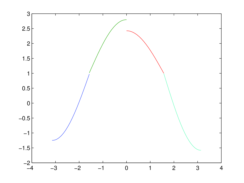
Figure 1.: Graphical solution of the ODE (4.1).

Remark 4.1 Notice that for each natural number $M>1$, one can easily modify this program in MathLab for obtaining a graphical solution of the differential equation (3.1)-(3.2) in $FD^{(2M)}([-l,l[\setminus G)$ whose coefficients $(A_{n}(x))_{0\leq n\leq 2M}$ are real-valued simple step functions on $[-l,l[$, $f$ is a trigonometric polynomial on $[-l,l[$ and $G$ is the partition of the interval $[-l,l[$ defined by the family $(A_{n}(x))_{0\leq n\leq 2M}$.

Remark 4.2 Since each constant $c$ admits the following evident representation c=c ×Ind_[-π,-π/2[(x)+c ×Ind_[-π/2,0[(x)+c ×Ind_[0,π/2[(x)+c ×Ind_[π/2, π[(x), we can use above mentioned program for a solution of the differential equation (2.3)-(2.4) with constant coefficients.

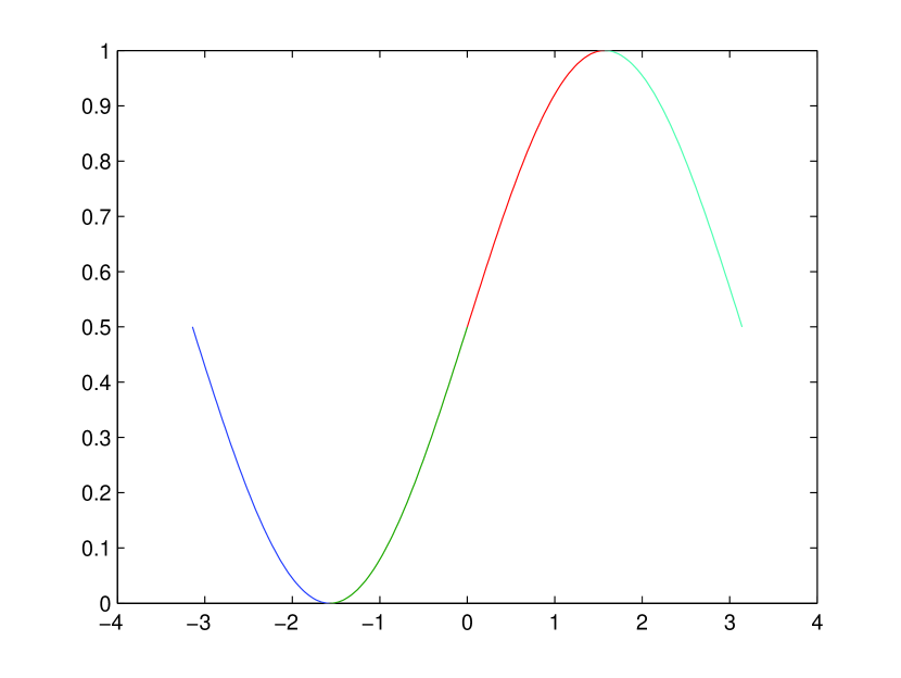
Figure 2.: Graphical solution of the ODE (4.4).

On Figure 2, the graphical solution of the linear non-homogeneous ordinary differential equation of the of the second order with real-valued constant coefficients

Ψ(x)-d2dx2Ψ(x)=1/2+cos(x), is presented, which has been obtained by entering in the above mentioned program of the following data:

$A1=[0,-1,0,0,0,0,0,0,0,0,0,0,0,0,0,0,0,0,0,0,0,0];$

$A2=[0,-1,0,0,0,0,0,0,0,0,0,0,0,0,0,0,0,0,0,0,0,0];$

$A3=[0,-1,0,0,0,0,0,0,0,0,0,0,0,0,0,0,0,0,0,0,0,0];$

$A4=[0,-1,0,0,0,0,0,0,0,0,0,0,0,0,0,0,0,0,0,0,0,0];$

$C=[0,0,0,0,0,0,0,0,0,0,0,0,0,0,0,0,0,0,0,0,0,0];$

$D=[1,0,0,0,0,0,0,0,0,0,0,0,0,0,0,0,0,0,0,0,0,0];$

$C0=1;~{}A10=1;~{}A20=1;~{}A30=1;~{}A40=1;$

Remark 4.1.

The approach of Theorem 3.4 used for a solution of (3.1)-(3.2) with real-valued simple step functions $(A_{n}(x))_{0\leq n\leq 2M}$ can be used in such a case when the corresponding coefficients are continuous functions on $[-l,l[$. If we will approximate these coefficients by real-valued simple step functions, then it is natural to wait that under some ”nice restrictions” on these coefficients the solution obtained by Theorem 3.4, will be a ”good approximation” of the corresponding solution.

References

• [1] Linear differential equation, http://en.wikipedia.org/wiki/Linear-differential-equation.
• [2] G.Birkhoff, G. Rota, Ordinary Differential Equations, New York: John Wiley and Sons, Inc., 1978.
• [3] J.C. Robinson, An Introduction to Ordinary Differential Equations, Cambridge, UK.: Cambridge University Press, 2004.
• [4] G.Pantsulaia, G.Giorgadze, On some applications of infinite-dimensional cellular matrices, Georg. Inter. J. Sci. Tech., Nova Science Publishers, Volume 3, Issue 1 (2011), 107-129.
• [5] A. Stanoyevitch, Introduction to MATLAB ยฎ with numerical preliminaries, Wiley-Interscience [John Wiley $\&$ Sons], Hoboken, NJ, 2005. x+331 pp.