Monte Carlo Method for Calculating Oxygen Abundances and Their Uncertainties from Strong-Line Flux Measurements

Abstract

We present the open-source Python code pyMCZ that determines oxygen abundance and its distribution from strong emission lines in the standard metallicity calibrators, based on the original IDL code of Kewley & Dopita (2002) with updates from Kewley & Ellison (2008), and expanded to include more recently developed calibrators. The standard strong-line diagnostics have been used to estimate the oxygen abundance in the interstellar medium through various emission line ratios (referred to as indicators) in many areas of astrophysics, including galaxy evolution and supernova host galaxy studies. We introduce a Python implementation of these methods that, through Monte Carlo sampling, better characterizes the statistical oxygen abundance confidence region including the effect due to the propagation of observational uncertainties. These uncertainties are likely to dominate the error budget in the case of distant galaxies, hosts of cosmic explosions. Given line flux measurements and their uncertainties, our code produces synthetic distributions for the oxygen abundance in up to 15 metallicity calibrators simultaneously, as well as for E(B-V), and estimates their median values and their 68% confidence regions. We provide the option of outputting the full Monte Carlo distributions, and their Kernel Density estimates. We test our code on emission line measurements from a sample of nearby supernova host galaxies ($z<0.15$) and compare our metallicity results with those from previous methods. We show that our metallicity estimates are consistent with previous methods but yield smaller statistical uncertainties. It should be noted that systematic uncertainties are not taken into account. We also offer visualization tools to assess the spread of the oxygen abundance in the different calibrators, as well as the shape of the estimated oxygen abundance distribution in each calibrator, and develop robust metrics for determining the appropriate Monte Carlo sample size. The code is open access and open source and can be found at https://github.com/nyusngroup/pyMCZ

1. Introduction

Small amounts of carbon, oxygen, nitrogen, sulfur, iron and other elements provide a splash of color to the otherwise dominating grayscape of hydrogen and helium in the stars and gas of galaxies. Nevertheless, even this minute presence of heavy elements is important for many areas of astrophysics. For example, Johnson & Li (2012) suggest that if it were not for the relatively high metallicity level in our Solar System, planet formation may not have been possible. With $Z$ representing the mass fraction of metals, all elements heavier than He (also collectively called metallicity), for our own Sun the value is measured to be $Z=0.0153$ (Caffau et al., 2011), though there are suggestions of a lower Solar metallicity of $Z=0.0134$ (Asplund et al., 2009; Grevesse et al., 2010). When properly observed and estimated, metallicity measurements of galaxies can tightly constrain models of galaxy formation and evolution (e.g., Kewley & Ellison 2008 and references therein), and shed light on the metallicity dependence and production conditions for different types of supernovae (SNe) and long-duration gamma-ray bursts (GRBs) (e.g., Modjaz et al. 2008; Levesque et al. 2010; Anderson et al. 2010; Modjaz et al. 2011; Kelly & Kirshner 2012; Sanders et al. 2012; Leloudas et al. 2014; Lunnan et al. 2014; Pan et al. 2014).

Metals are produced in the cores of massive stars during their fusion life cycle but also during the extreme conditions of stellar explosions. For example, the majority of iron is synthesized in thermonuclear explosions (SNe Ia) while nearly all oxygen and other $\alpha$-elements are released in various kinds of core-collapse SNe (SNe II and stripped-envelope core-collapse SNe).

However, for almost all astronomical objects, metallicity cannot be measured directly. The oxygen abundance in the gas-phase is the canonical choice of metallicity indicator for interstellar medium (ISM) studies. After Hydrogen, Oxygen lines are the strongest emission lines in optical wavelengths. Oxygen is the most abundant metal and it is only weakly depleted onto dust grains, in contrast to refractory elements such as magnesium, silicon, or iron (iron for example is depleted by more than a factor of 10 in Orion; see Simón-Díaz & Stasińska 2011). The oxygen abundance is expressed as $12+\log_{10}(O/H)$, where O and H represent the number of oxygen and hydrogen atoms, respectively. For example: Caffau et al. 2011 measure a Solar oxygen abundance of $12+\log_{10}(O/H)$= 8.76 $\pm$ 0.07, while Asplund et al. (2009) suggest $12+\log_{10}(O/H)$= 8.69. While oxygen abundance is used to gauge metallicity, in many cases in the literature, including here, the terms metallicity and oxygen abundance are used interchangeably. Importantly, oxygen exhibits very strong nebular lines in the optical wavelength range in spectra of HII regions (e.g., Pagel et al. 1979; Osterbrock 1989; Tremonti et al. 2004), which can be measured. Thus, many different diagnostic techniques relying on different lines of oxygen, hydrogen and other elements, have been developed (e.g., Kewley & Dopita 2002 – hereafter KD02, Pettini & Pagel 2004 – PP04, Kobulnicky & Kewley 2004 – KK04, Kewley & Ellison 2008 – KE08), and are discussed in the next section.

Many fields rely on the determination of the metallicity environments to understand physical phenomena, such as SN and planetary formation, from a causal, and possibly mechanicistic point of view. However many of these fields, including SN studies, have used metallicity calibration techniques somewhat acritically, at times inferring from calibrators that are not comparable, as they rely on different assumptions, because of the scarsity of complete dataset that would allow consistent estimates, and often ignoring many sources of uncertainty.

The purpose of this paper is to present a public code that collects different abundance diagnostics to efficiently and rapidly compute metallicity from strong emission line fluxes as well as the associated statistical uncertainties due to the measured emission line flux uncertainties. This source of uncertainty is particularly relevant in the study of SN metallicity environments, since the host galaxies of these cosmics explosions are often at large distances. While in many other contexts the signal-to-noise (SNR) of the spectra themselves may contribute negligebly to the total uncertainty budget, compared for example to errors in the model parameters, it is often a substantial source of uncertainty for high $Z$ galaxies that host SNe. The necessity to compute metallicity quickly, and systematically for large samples arises from the new availability of large samples, enabled by IMACS spectrographs for example, and collected by surveys such as MANGA (Bundy et al., 2015).

Our open-source Python package is named pyMCZ. This Python code allows the user to quickly produce metallicity values with sensible confidence regions for several metallicity calibrators at once, given an input set of spectral line measurements and their errors, and to obtain and visualize the distribution of metallicities. pyMCZ is structured in a modular way in order to allows the user to include other strong line metallicity calibration methods, and link to external code packages, with minimal modifications, and naturally extend the advantages of the Monte Carlo (MC) based propagation of the observational uncertainties to the newly included calibrators. While we do not mean to advocate for a particular metallicity calibrator to be adopted, the comparison of multiple calibrator outputs, and the shape of each metallicity distribution, can guide the user in understanding the reliability of a metallicity estimate, given a set of line fluxes. Below we describe the different oxygen abundance diagnostics, and our Python module implementation.

2. Oxygen abundance diagnostics and calibrators

In this section we present a brief overview of the various observational methods for measuring the gas-phase oxygen abundance - however, for a detailed discussion, and to understand the many caveats, we encourage the reader to read the reviews by, e.g., Stasińska (2002), KE08, Moustakas et al. (2010), Stasińska (2010), López-Sánchez et al. (2012), Dopita et al. (2013), hereafter D13, and Blanc et al. (2015).

The so-called “classical” way to estimate oxygen abundances is the electron temperature ($T_{e}$) method, which estimates the electron temperature and density of a nebula using a number of oxygen lines in different ionization states, including the auroral [O III] $\lambda$4363 line, to then directly estimate the O II and O III abundances and finally, after correcting for the unseen stages of ionization, to obtain the total oxygen abundance. However, except for low-metallicity environments, the auroral [O III] $\lambda$4363 line is very weak, and it saturates at metallicities higher than solar (Stasińska, 2002), since at higher metallicities the cooling is dominated by the oxygen fine structure lines in the near-infrared (NIR). In addition, there are other caveats about the $T_{e}$-method, as fluctuations and gradients in temperature or in chemical composition may lead to underestimates of the oxygen abundance (see for example Peimbert 1967, and López-Sánchez et al. 2012). Most recently, Berg et al. (2015) suggested that among the auroral lines [O II], [O III] and [N II], the [O III] $\lambda$4363 line, commonly used for $T_{e}$ measurements, is the most problematic one, giving rise to temperature discrepancies. Thus, other methods have been developed that estimate the oxygen abundance from ratios of strong nebular lines in the spectra of HII regions, including amongst others [O III] $\lambda\lambda$ 4959, 5007, [O II] $\lambda\lambda$ 3726, 3729, [N II] $\lambda$ 6584, [S II] $\lambda\lambda$ 6717, 6731, as well as H$\alpha$ and H$\beta$. These are called strong-line calibrations and are the subject of this manuscript.

Strong-line methods can be categorized into three types, depending on how they calibrate the observed emission line ratios:

• empirical methods, which calibrate line ratios on observed $T_{e}$-based metallicities (e.g., Pilyugin & Thuan 2005 – hereafter P05; Pilyugin et al. 2010 – P10; Pilyugin et al. 2012 – P12; Marino et al. 2013 – M13),

• theoretical methods, which rely on calibrating various observed line ratios using stellar population and photoionization models (basically theoretically simulating HII regions, e.g., McGaugh 1991 – hereafter M91, KD02, Tremonti et al. 2004)

• and lastly hybrid methods that use a mixture of both empirical and theoretical calibrations (e.g., Denicoló et al. 2002 – hereafter D02, Pettini & Pagel 2004 – PP04; Maiolino et al. 2008 – M08; and Pérez-Montero 2014 – PM14).

The ionization parameter $q$ needs to be taken into account in all calibrations, as HII regions at the same metallicity but with different ionization parameters produce different line strengths. The importance of the ionization parameter, which can be physically understood as corresponding to the maximum velocity of an ionized front that can be driven by the local radiation field of hot massive stars that are ionizing the ISM gas, was demonstrated in a number of works including Evans & Dopita 1985; Dopita & Evans 1986, KD02, PM14, and Sánchez et al. 2015. All calibrations include its impact, either implicitly (by assuming the input object has the same values as the calibration sample) or by explicitly solving for it.

While historically there have been large systematic offsets between the $T_{e}$ method and the strong line methods, partially due to real temperature gradients that exist in the high-ionization zones of the HII regions (López-Sánchez et al., 2012), D13 demonstrated that the results of the $T_{e}$ method and strong line methods are reconciled if the energy distribution of the electrons in the HII regions is not assumed to be a simple Maxwell-Boltzmann distribution (as in prior works), but a more realistic $\kappa$ distribution (Vasyliunas, 1968; Owocki & Scudder, 1983), as observed in Solar plasma. In addition they find that the effect of changing the specific $\kappa$ distribution on the strong-line methods is minor (see also Mendoza & Bautista 2014).

There is a long-standing debate about which diagnostic to use, and there are systematic metallicity offsets between different methods (recombination lines vs. strong-line method vs. the “direct” $T_{e}$ method), however, the relative metallicity trends can be considered robust, if the analysis is performed self-consistently in the same calibrator, and trends are seen across different calibrators (KD08, Moustakas et al. 2010). It is of course necessary to estimate uncertainties for the relative comparisons to be meaningful. Note that while conversion values between different calibrators (Kewley & Ellison, 2008) have been estimated, they are average quantities derived from large data sets (tens of thousands of SDSS galaxies), and they should be used with caution, if at all, on individual metallicity measurements.

3. Commonly Used metallicity indicators

Line ratios commonly used as metallicity indicators (used in PP04, P05, P12, and M13) are

$$N2~{}=~{}\frac{\mathrm{[N~{}II]}\lambda 6584}{\mathrm{H}\alpha}$$

and the $O3N2$ index, first introduced by Alloin et al. (1979) and defined as $O3/\mathrm{H}\beta/N2$ where $O3/\mathrm{H}\beta~{}=~{}\frac{\mathrm{[O~{}III]}\lambda 4959+\mathrm{[O~{}III]}\lambda 5007}{\mathrm{H}\beta}$, thus:

$$O3N2~{}=~{}\frac{\mathrm{[O~{}III]}\lambda 4959+\mathrm{[O~{}III]}\lambda 5007}{\mathrm{H}\beta}\times\frac{\mathrm{H}\alpha}{\mathrm{[N~{}II]}\lambda 6584}.$$

Since $N2$ employs two closely spaced lines ($\mathrm{H}\alpha$  and [N II]$\lambda 6584$), their ratio is not affected by stellar absorption or (uncertain) reddening, and they are easily observed in one simple spectroscopic setup. Thus the PP04 calibration based on $N2$ has become a popular calibrator to use for low-$z$ SN host galaxy studies (see meta-analyses by Sanders et al. 2012; Modjaz 2012; Leloudas et al. 2014 and others). However, it is important to note that the PP04-N2 calibration has a number of short-comings: the PP04 calibration implicitly assumes the same relationship between the line ratios and the ionization parameter as in the calibration sample from which it was initially derived, which includes only 137 extragalactic HII regions, and it is a hybrid calibration method. An updated calibration by M13 is based on a sample of HII regions almost three times larger than that of PP04 and, more importantly, only uses $T_{e}$-based metallicities. M13 finds a significantly shallower slope in the relationship between the $N2$ and $O3N2$ indices and the oxygen abundance. Our code outputs M13 as a default, and PP04 if explicitly requested. It is important to note that the employed nitrogen emission line saturates at high metallicity, and thus the $N2$ methods, including M13, fail at high-metallicity galaxies – at $12+\log_{10}(O/H)>8.8$ (KD08).

Additional strong line indicators include the $N2O2$ ratio:

$$N2O2~{}=~{}\frac{[N~{}II]~{}\lambda 6584}{[O~{}II]~{}\lambda 3727},$$

introduced by KD02, which exploits the leverage offered by the large diatance in wavelength of the $[N~{}II]~{}\lambda 6584$ and $[O~{}II]~{}\lambda 3727$ lines, but is then very sensitive to reddening and thus requires the measurements of $\mathrm{H}\alpha$ and $\mathrm{H}\beta$ to be available, and the Oxygen based $O3O2$ indicator:

$$O3O2=\frac{\mathrm{[O~{}III]}\lambda 4959+\mathrm{[O~{}III]}\lambda 5007}{\mathrm{[O~{}II]}\lambda 3727},$$

already introduced by M91, which has the obvious advantage of using only Oxygen lines, which are, as mentioned, the strongest emission lines in optical wavelengths apart from Hydrogen.

The ratio of oxygen line fluxes to $\mathrm{H}\beta$ is referred to as $R_{23}$ (Pagel et al., 1979):

$$R_{23}=\frac{\mathrm{[O~{}II]}\lambda 3727~{}+~{}\mathrm{[O~{}III]}\lambda\lambda 4959,5007}{\mathrm{H}\beta},$$

where [O III] $\lambda\lambda$ 4959,5007 stands for the sum of the two [O III] lines. This popular indicator is double-valued with metallicity: the same $R_{23}$ value may correspond to two metallicity values, and thus other indicators need to be used to break the degeneracy between the high (“upper branch”) and the low values (“lower branch”) of the $R_{23}$ metallicities (e.g., KD08, Moustakas et al. 2010). A similarly double valued indicator is $S_{23}$, which is based on the sulfure lines: $S_{23}=(\mathrm{[S~{}II]}~{}\lambda 6717+\mathrm{[S~{}III]}~{}\lambda 9069)/\mathrm{H}\beta$. For these double-values indicators the curvature of the relationship between the line ratio and the metallicity in the two branches depends on the ionization parameter, and both empirical and theoretical calibrators that use them have to solve for $q$. For the theoretical strong-line method, calibrations of $R_{23}$ by M91, KD02, and D13 use different theoretical photoionization models: different stellar populations codes (e.g., Starburst 99, based on Bruzual A. & Charlot 1993, or POPSTAR, Mollá et al. 2009) and photoionization codes (e.g., MAPPINGS Allen et al. 2008, or CLOUDY, Ferland et al. 1998) to calibrate different line ratio indices. M91 and KD02 use an iterative process to break the $R_{23}$ degeneracy and to constrain the ionization parameter $q$. Other calibrations, such as Z94, do not explicitly solve for $q$. On the empirical calibrators side, P10 introduces the $P$ parameter, which is a modified version of the ionization parameter $q$.

As can be seen, each calibrator has different advantages and disadvantages and should be used in different metallicity regimes (see detailed discussion in, for example, KD02, Stasińska 2002, KD08, Moustakas et al. 2010; López-Sánchez et al. 2012, D13, Blanc et al. 2015). Thus, pyMCZ outputs the oxygen abundance in the main metallicity calibrators whenever the lines necessary to calculate the indicators used by each method are available. As default output values for 11 metallicity diagnostics are generated (version v1.3, Fall 2015). By “diagnostics” here we mean a suite metallicity calibrators described in a single paper (e.g. KD02), and some of these diagnostics describe multiple calibrators based on different indicators: the KD02 diagnostic have four outputs and the PP04, P10, M13 , M08, and D13 diagnostic have multiple outputs as well.

4. pyMCZ: a python module for strong-line metallicity diagnostics

Figure 1.— Metallicity and reddening E(B-V)  parameter distributions based on the example data shown in Table 2: emission line data of the HII regions at the position of SN 2008D, published in Modjaz et al. 2011 (see section 5 for a discussion of the test sample). The distributions are generated from $N$=2,000 samples. The median values are shown with dashed white lines, while the confidence region, between the 16^th and the 84^th percentile is shaded in orange. We show the metallicity calibrators from Pettini & Pagel (2004), using [O III] and [N II] (PP04_O3N2), the $R_{23}$-based calibrator described in Kobulnicky & Kewley (2004) (KK04_$R_{23}$), and the combined calibrator of Kewley & Dopita (2002) (KD02_comb), updated as described in Kewley & Ellison (2008). Similar plots are outputted by the code for all computed metallicity calibrators. We note PP04 calibrators are an optional outputs of our code, since they are superseded by M13 (see section 2). However, we use them for comparison with the results obtained in Modjaz et al. 2011. Each plot indicates the calibrator, the sequential number of measurement in the input file (here “measurement 1 of 2”, which corresponds to the first line of the input ASCII files), the median, 16^th and 84^th percentile values, the sample size (which is by default initially set to 10% larger than the requested $N$ value, but can be smaller if some simulations lead to invalid metallicities), and, finally, the method used to choose the bin size for the histogram (Kuth’s rule in this case, see subsubsection 4.3.1).

We developed a Python package, pyMCZ for the simultaneous calculation of $12+\log_{10}(O/H)$  in various calibrators, and its confidence region. We started with the iterative IDL code by KD02 hereafter referred to as IDLKD02, specifically a version updated in KE08. We translated the code into Python and added new, more recent calibrators (see subsection 4.2) and new features, of which the most important is the capability of obtaining uncertainties on the metallicity outputs via MC sampling.

4.1. Availability and Technical details

The source code is published under MIT-license on GitHub. At this time the code is released under DO I: 10.5281/zenodo.17880 and the most recent stable version is version 1.3: p̱yMCZ v1.3. Project details, step-wise tutorials, and further information can be found in the module README. Development is done in Linux and OS X. The package requires standard python packages, such as numpy, scipy, pylab, and additional features are enabled if the packages astroml, skitlearn, and pyqz are installed, but these packages are not required. pyMCZ can be run as a standalone package from the local directory, or it can be installed (via python setup.py install).

4.2. Input and Output of code

Table 1calibrators and line ratios/indicators from which the calibrators are derived

Calibrator	Lines used for metallicity calculation	Support lines and calibrators	Reference
M91	$R_{23}$, $O3O2$	$N2$, $N2O2$	McGaugh (1991)
Z94*	$R_{23}$	-	Zaritsky et al. (1994)
(DP00*)	$S_{23}$	-	Díaz & Pérez-Montero (2000)
(P01)	$R_{23}$, $O3/\mathrm{H}\beta$, $\mathrm{[O~{}II]}\lambda 3727/\mathrm{H}\beta$	$N2$, $N2O2$	Pilyugin (2001)
(C01_R23)	$R_{23}$, ${\mathrm{[O~{}III]}\lambda 5007}/{\mathrm{H}\beta}$, $\frac{\mathrm{[O~{}II]}\lambda 3727}{\mathrm{[O~{}III]}\lambda 5007}$	-	Charlot & Longhetti (2001)
(C01_N2S2)	$R_{23}$, $\frac{\mathrm{[O~{}II]}\lambda 3727}{\mathrm{[O~{}III]}\lambda 5007}$, $\frac{\mathrm{[N~{}II]}\lambda 6584}{\mathrm{[S~{}II]}\lambda 6717}$	-	Charlot & Longhetti (2001)
D02*	$N2$	-	Denicoló et al. (2002)
KD02_N2O2*	$N2O2$	-	Kewley & Dopita (2002)
(PP04_N2Ha*)	$N2$	-	Pettini & Pagel (2004)
(PP04_O3N2*)	$N2$, $O3/\mathrm{H}\beta$	-	Pettini & Pagel (2004)
KK04_N2Ha	$N2$, $q$	$N2O2$	Kobulnicky & Kewley (2004)
P05	$R_{23}$, $O3/\mathrm{H}\beta$, ${\mathrm{[O~{}II]}\lambda 3727}/{\mathrm{H}\beta}$	$N2$, $N2O2$	Pilyugin & Thuan (2005)
KK04_$R_{23}$	$R_{23}$, $q$,	$N2$, $N2O2$	Kewley & Ellison (2008)
KD02_comb	M91, KD02_N2O2, KD02_N2Ha, KD04_R23	$N2$, $N2O2$	Kewley & Ellison (2008)
M08_O3O2	$O3O2$	-	Maiolino et al. (2008)
M08_N2Ha	$N2$	-	Maiolino et al. (2008)
M08_R23	$R_{23}$	M08_O3O2, M08_N2Ha	Maiolino et al. (2008)
(M08_O3Hb)	${\mathrm{[O~{}III]}\lambda 5007}/{\mathrm{H}\beta}$	M08_O3O2, M08_N2Ha	Maiolino et al. (2008)
(M08_O2Hb)	${\mathrm{[O~{}II]}\lambda 3727}/{\mathrm{H}\beta}$	M08_O3O2, M08_N2Ha	Maiolino et al. (2008)
(M08_O3N2)	$\frac{\mathrm{[O~{}III]}\lambda 5007}{\mathrm{[N~{}II]}\lambda 6584}$	M08_O3O2, M08_N2Ha	Maiolino et al. (2008)
P10_ON	$N2$, $O3/\mathrm{H}\beta$, ${\mathrm{[O~{}II]}\lambda 3727}/{\mathrm{H}\beta}$	-	Pilyugin et al. (2010)
P10_ONS	${\mathrm{[N~{}II]}\lambda 6584}/{\mathrm{H}\beta}$, $O3/\mathrm{H}\beta$	-	Pilyugin et al. (2010)
	${\mathrm{[O~{}II]}\lambda 3727}/{\mathrm{H}\beta}$, $\frac{\mathrm{[S~{}II]}\lambda 6717+\mathrm{[S~{}II]}\lambda 6731}{\mathrm{H}\beta}$
M13_N2*	${\mathrm{[N~{}II]}\lambda 6584}/{\mathrm{H}\beta}$	-	Marino et al. (2013)
M13_O3N2*	${\mathrm{[N~{}II]}\lambda 6584}/{\mathrm{H}\beta}$, $O3/\mathrm{H}\beta$	-	Marino et al. (2013)
D13_N2S2_O3S2	$\frac{\mathrm{[N~{}II]}\lambda 6584}{\mathrm{[S~{}II]}\lambda 6717+\mathrm{[S~{}II]}\lambda 6731}$, $\frac{\mathrm{[O~{}III]}\lambda 5007}{\mathrm{[S~{}II]}\lambda 6717+\mathrm{[S~{}II]}\lambda 6731}$	-	Dopita et al. (2013)
D13_N2S2_O3Hb	$\frac{\mathrm{[N~{}II]}\lambda 6584}{\mathrm{[S~{}II]}\lambda 6717+\mathrm{[S~{}II]}\lambda 6731}$, $O3/\mathrm{H}\beta$	-	Dopita et al. (2013)
D13_N2S2_O3O2	$\frac{\mathrm{[N~{}II]}\lambda 6584}{\mathrm{[S~{}II]}\lambda 6717+\mathrm{[S~{}II]}\lambda 6731}$, $O3O2$	-	Dopita et al. (2013)
D13_N2O2_O3S2	$N2O2$, $\frac{\mathrm{[O~{}III]}\lambda 5007}{\mathrm{[S~{}II]}\lambda 6717+\mathrm{[S~{}II]}\lambda 6731}$	-	Dopita et al. (2013)
D13_N2O2_O3Hb	$N2O2$, $O3/\mathrm{H}\beta$	-	Dopita et al. (2013)
D13_N2O2_O3O2	$N2O2$, $O3O2$	-	Dopita et al. (2013)
D13_N2Ha_O3Hb	$N2$, $O3/\mathrm{H}\beta$	-	Dopita et al. (2013)
D13_N2Ha_O3O2	$N2$, $O3O2$	-	Dopita et al. (2013)

The input of the code is a set of spectral emission line fluxes. We assume that the observed emission lines originate in HII regions and are not due to non-thermal excitation by, for example, AGN, interstellar shocks from SNe, or stellar winds. Tests to exclude data contaminated by such non-thermal sources should be executed prior to running this code using the recommended indicators by, e.g., Baldwin et al. (1981), Kauffmann et al. (2003), Kewley et al. (2006), and Cid Fernandes et al. (2010); Sánchez et al. (2015). Furthermore, these lines should have all the correct flux calibration (at least correct relative calibration) and should have a SNR of at least 3. The latter requirement is important for the success of the sampling technique. In our code, synthetic line flux measurements are drawn within a Gaussian distribution with standard deviation equal to the measurement error, and centered on the measured flux value (subsection 4.3). Thus, a $\mathrm{SNR}>=3$ assures that fewer than $\sim 1\%$ of the sampled fluxes fall below zero (and are thus invalid). The code checks if for any line the $\mathrm{SNR}>=3$ condition is not satisfied, and issues a warning message.

Emission line flux values are fed into our Python implementation as in the original IDLKD02 code. The inputs are emission line flux values, and their uncertainties, for the following lines: $\mathrm{H}\alpha$, $\mathrm{H}\beta$, [O I] $\lambda$ 6300, [O II] $\lambda$ 3727, [O III] $\lambda$ 4959, [O III] $\lambda$ 5007, [N II] $\lambda$ 6584, [S II] $\lambda$ 6717, [S II] $\lambda$ 6731, [S III] $\lambda$ 9096 and [S III] $\lambda$ 9532. The latter two lines can be used to calculate the sulfur ratio $S_{23}$, but are not often observed since they are in the NIR. Only one metallicity calibrator based on $S_{23}$, Díaz & Pérez-Montero 2000 (DP00), is implemented in the current version of the code. The line fluxes are to be stored in an ASCII file, and the measurement errors in a separate ASCII file (for consistency with the original IDLKS02 code; consult the README.md in the GitHub repository for details about the input format, and find example files in the repository). If the fluxes for the specified lines are not available, the entry should be set to NaN. The oxygen abundance will be calculated only for metallicity calibrators that use valid, non-NaN, line fluxes. If the line fluxes necessary for specific calibrators are not provided, the output metallicities will default to NaN. In absence of measurement uncertainties, the error should be set to 0.0 in the input ASCII file. If the errors in the measurements are not provided, the code will specify that it cannot create a measurement distribution or determine a confidence interval, but it will calculate and output the nominal metallicity obtained from the input flux measurement.

The inputted line fluxes are corrected for reddening by using the observed Balmer decrement, for which $\mathrm{H}\alpha$  and $\mathrm{H}\beta$  flux values need to be provided. We assume case B recombination, and thus the standard value of 2.86 as the intrinsic $\mathrm{H}\alpha$/$\mathrm{H}\beta$  ratio (Osterbrock, 1989), and apply the standard Galactic reddening law with $R_{V}$ = 3.1 (Cardelli et al., 1989). However, the user can choose other extinction laws and $R_{V}$ values, if desired, given the code’s open-source nature. If the input measurements are already de-reddened, the user can disable the reddening correction. If either $\mathrm{H}\alpha$  or $\mathrm{H}\beta$  are not provided, the reddening correction cannot be implemented. The user is notified with a warning message and has the option to proceed with the calculations with uncorrected line fluxes. This option is enabled, and should of course only be chosen, for cases in which the spectral fluxes are already dereddened before being fed is input to pyMCZ.

We implement the calculation of $12+\log_{10}(O/H)$  values and their uncertainties from the metallicity calibrators listed below, and summarized in Table 1, implemented as prescribed in KE08 where not otherwise noted. We emphasize that subsets of these calibrators use the same input line ratios, and that related assumptions and similar observation and simulations are used to generate the calibrator algorithms (e.g. there are several calibrators that are essential linear or near-linear functions of $N2$: PP04_N2, KK04_N2 and M13_N2). Thus the oxygen abundance results produced using different calibrator are far from independent.

• M91 (McGaugh, 1991) is an $R_{23}$-based theoretical calibrator which also determines the ionization parameter. To break the $R_{23}$ degeneracy we use $N2O2$, following KE08 Appendix 2.

• Z94 (Zaritsky et al., 1994) which is valid for the upper branch of $R_{23}$ only, and we conservatively constrain it to log($R_{23})<0.9$, the range that is covered by the photoionization model grids.

• D02 (Denicoló et al., 2002) for which we include, in addition to the uncertainties in the measurements, the uncertainty in the fit parameters as they appeared in the original paper.

• P05 (Pilyugin & Thuan, 2005) an $R_{23}$-based method calibrated via $T_{e}$ metallicities on a sample of HII regions. We use the values of $N2O2$, and $N2$ to discriminate between upper and lower branch.

• KD02 & KK04: 4 calibrators: KD02_N2O2, which uses the $N2O2$ indicator  (Kewley & Dopita, 2002), KK04_N2$\mathrm{H}\alpha$  which uses the N2 indicator (Kobulnicky & Kewley, 2004), KK04_$R_{23}$ (Kewley & Ellison 2008, appendix A2.2), which is based on the value of $R_{23}$, and a combined method, KD02_comb that chooses the optimal method given the input line fluxes and is implemented as described in Appendix 2.3 of Kewley & Ellison (2008).

• M08 (Maiolino et al., 2008): This calibrator is a combination of the KD02 photoionization models at high metallicities and $T_{e}$ based metallicities at low metallicities. Our default output includes their strong line diagnostic, which is based on $R_{23}$, and the diagnostics based on $O3O2$ and [N II]/$\mathrm{H}\alpha$, since the metallicity estimates from [N II]/$\mathrm{H}\alpha$  or $O3O2$ are necessary to resolve the degeneracy in the double-valued $R_{23}$ metallicity. The other calibrators (based on [O II]/$\mathrm{H}\beta$, [O III]/$\mathrm{H}\beta$, and [O III]/[N II]) can be outputted upon explicit user request, via the command line options.

• P10 (Pilyugin et al., 2010): This is the so-called ONS diagnostic (involving the [O II], [O III], [N II] and [S II] lines) and is calibrated with HII regions that have $T_{e}$ based metallicities.

• M13 (Marino et al., 2013): Two calibrators: M13_N2, which is a linear fit to the $\mathrm{[N~{}II]}~{}\lambda 6584/\mathrm{H}\alpha$, and M13_O3N2. This is an updated calibration of the PP04 $O3N2$ method, based on a large number of $T_{e}$-based metallicity measurements, including those from the Calar Alto Legacy Integral Field spectroscopy Area survey (CALIFA, Sánchez et al. 2012, almost three times larger than the sample used in PP04). This method derives a significantly shallower slope between the $O3N2$ index and the oxygen abundance than the PP04 calibration did.

• D13: (Dopita et al., 2013). The photoionization models used in KD02 and in KK04 are updated by including new atomic data within a modified photoionization code and by assuming a $\kappa$ distribution for the energy of the electrons in the HII regions, rather than the simple Maxwell-Boltzmann distribution assumed in prior works. This distribution is more realistic, as observed in Solar plasma (Nicholls et al., 2012). If the user has installed the publicly available pyqz Python module, [N II], [S II], [O III], $\mathrm{H}\alpha$, and $\mathrm{H}\beta$  lines are fed to the pyqz module, which produces up to eight emission line ratio diagnostics for $12+\log_{10}(O/H)$, each using two of the indicators [N II]/[S II], [N II]/$\mathrm{H}\alpha$, [O III]/[S II], and [O III]/$\mathrm{H}\beta$. Our code sets the $\kappa$ parameter to 20, which is the value that D13 found best resolves the inconsistencies between oxygen abundance values derived from the strong-line methods and from the “direct” $T_{e}$ method.

• DP00, P01, C01 & PP04 (only upon request): (Díaz & Pérez-Montero 2000, Pilyugin 2001, Charlot & Longhetti 2001). DP00 is based on $S_{23}$, and is the only $S_{23}$ calibrator implemented in the current version of the code. P01 is superseded by P05. C01 produces a diagnostic based on $R_{23}$, C01_$R_{23}$, and one based on [N II]/[S II], C01_N2S2; C01_$R_{23}$ was used to calculate the combined calibrator described in KK04, and included in the IDLKD02 code, but it is no longer used in the new combined calibrator KD02_comb, which supersedes the old one. Thus, P01 and C01 are only included for historical reasons. PP04: (Pettini & Pagel, 2004) includes two calibrators PP04_N2, based on the [N II]/$\mathrm{H}\alpha$  ratio, and PP04_O3N2, based on ($\frac{\mathrm{[O~{}III]}}{\mathrm{H}\beta}/\frac{\mathrm{[N~{}II]}}{\mathrm{H}\alpha}$). calibrators are commonly used in the literature investigating SN and GRB environments (see Modjaz et al. 2011 and referenced therein). They are superseded by the M13 calibrators (see section 2), but are included here for completeness. These five calibrators are not part of the default output of our code, however they are still available upon explicit user request via command line input.

The following diagnostics were calculated in the original IDLKD02 code, and are discussed in detail in KD02 and Kewley & Ellison (2008): C01, P01, M91, Z94, D02, PP04, P05, KD02, KK04, and KD02_comb. We refer the reader to those papers for further details. DP00 is the only diagnostic that relies on sulfur ratios $S_{23}$. The shortcomings of $S_{23}$ as a tool to measure abundances are discussed in KD02. The DP00 diagnostic we implement is modified with the addition of a term $\propto(c+S_{23}^{3})^{-1}$ as suggested by KD02, which corrects the tendency of the calibrator to systematically underestimate the abundance, with a discrepancy growing larger at higher metallicity. However, we point out that the scatter in metallicity derived from this diagnostic compared to others remains high.

The distributions of E(B-V) and $\log(R_{23})$ values are also part of the default output. Certain parameters, such as the ionization parameter $q$ and the electron density (using the [S II] lines) are computed as long as the necessary lines are provided, but are not outputted in the current version of our code $-$ however, since the code is open-source, the reader can easily modify the code to suit their needs.

4.3. Computing Statistical Uncertainties

Three kinds of uncertainties must be taken into account when calculating metallicities: 1) the propagation of measurements errors of the line fluxes; 2) the propagation of uncertainty in the calibration (either from model-fitting or propagating the uncertainties of the coefficients in the linear calibrations); 3) the systematic offsets/errors between different calibrations with respect to the “true” value of the metallicity.

In our work we account for errors due to the emission line measurement uncertainties, and, when provided by the authors, to the calibration uncertainties, and propagate them into the derived metallicities. The propagation of the observational errors cannot, in most cases, be conducted analytically, since many metallicity calculations rely on, for example, decision trees. Thus the MC environment is necessary in most cases to properly assess the effect of the measurement uncertainties, and, for consistency and to generate a simple, modular code, we adopt it as the method for uncertainty calculation in all cases. We provide the full metallicity distributions, for all calculated calibrators. The latter is important since, as we show, metallicity distributions are usually not symmetric and can be multimodal (for example for the $R_{23}$ based calibrators). In addition, we provide the full metallicity parameter distribution to the user. We note that we do not address the third source of uncertainty: any systematic errors between different calibrators. This is the subject, for example, of López-Sánchez et al. (2012).

For every set of input line measurements we introduce a MC sampling method to obtain iterations via random sampling within the measurement uncertainties, and thus we obtain a robust result for statistical error estimation (e.g., Efron 1979; Hastie et al. 2009; Andrae 2010). Given a dataset with error bars from which certain parameters are estimated, MC sampling generates synthetic data samples from a given distribution. We draw synthetic data from a Gaussian distribution centered on each measured line flux value, with standard deviation corresponding to the measurement uncertainty. The implicit assumption is made that the line flux error is Gaussian distributed in nature, and that the errors are independent. However, the user who wishes to provide their own probability distribution for the emission line uncertainties can easily modify the code to include the desired distribution. For each metallicity calibrator, and for each of the $N$ values chosen randomly within the relevant emission line distributions, we run the calculations that compute the metallicity. By generating synthetic data, this method effectively simulates conducting multiple experiments when repeating observations is impractical or impossible, as is the case of the emission line flux data.

The sample size $N$ is set by the user, and one should expect an appropriate value of $N$ to be a few 1000s, depending on the metallicity calibrator chosen and measurement errors (for example: $N=2,000$ is determined to be sufficient for our example data, as shown in subsection 4.4).

A distribution of parameter estimates for the oxygen abundance is generated, from which the median metallicity and its confidence region are calculated, and the results are binned and visualized in an outputted histogram (see subsubsection 4.3.1). This is done for each calibrator the user chooses to calculate. The fiftieth (50%) percentile, i.e. the median, is reported as the estimated metallicity value, and the 16^th and 84^th percentiles of the metallicity estimate distribution, as its confidence region. The user can also choose to output the full metallicity distribution as binary or ASCII files.

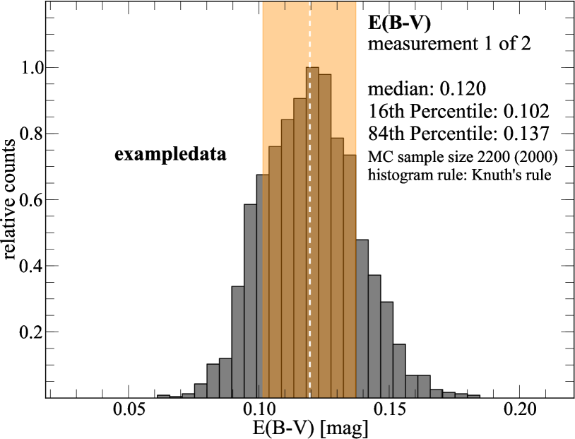
This MC sampling approach takes into account the impact of the uncertain reddening (due to the uncertainties in the measurement of the $\mathrm{H}\alpha$ and $\mathrm{H}\beta$ fluxes), when the option for de-reddened metallicities is chosen. For each synthetic set of measurements, a new reddening value is calculated based on the sampled $\mathrm{H}\alpha$ and $\mathrm{H}\beta$ fluxes, and used to compute the de-reddened metallicity value, so that the derived distribution of metallicity values naturally takes into account the uncertainty in reddening. The median value, and confidence intervals for E(B-V), as well as a distribution histogram, are outputted together with the metallicity calibrators (first panel in Figure 1). If either $\mathrm{H}\alpha$ or $\mathrm{H}\beta$ are not provided, however, no reddening correction can be applied. The computed metallicity will not be reddening-corrected and the E(B-V) output will be set to zero.

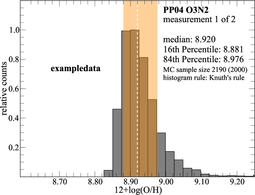
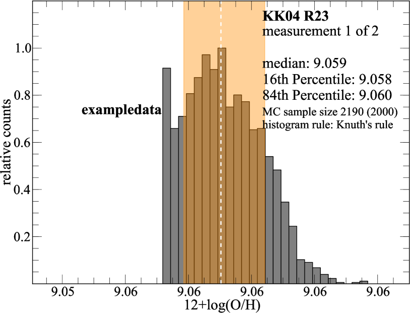
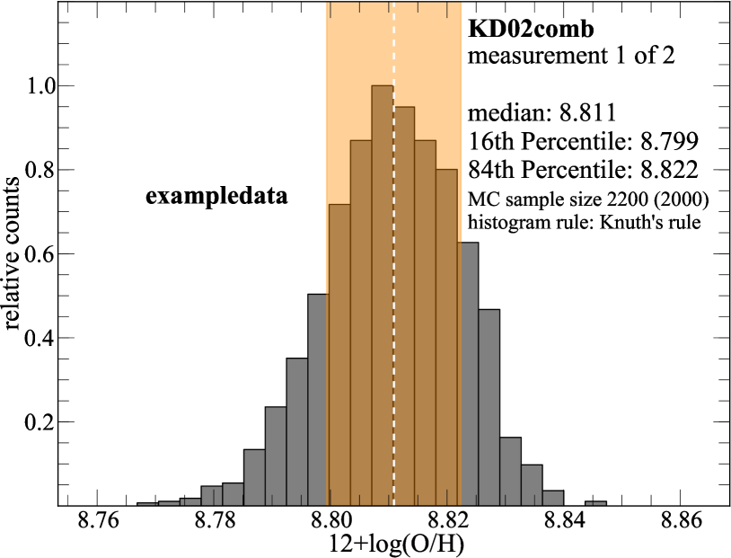
Figure 1 shows metallicity estimate distributions for three representative calibrators (PP04_O3N2, KK04_$R_{23}$, and KD02_comb), and for the reddening parameter E(B-V). Similar plots are produced for all calibrators calculated and for $\log(R_{23})$ as a default output (and are available online in the pyMCZ GitHub repository). Although the input line flux distributions are Gaussian, the metallicity distributions are not, for two reasons: first, since the metallicities are computed based on log values of line flux ratios, symmetric error bars in linear space will translate into asymmetric error bars in log space; and second, some metallicity calibrator computations are non-linear, and sometimes bimodal, especially those that use $R_{23}$ and $S_{23}$, as shown in Figure 2, since the upper or lower branch metallicity value has to be chosen to break the degeneracy for each synthetic measurement.

Figure 2.— Metallicity distribution according to the KK04_$R_{23}$ calibrator for the site of SN 2007rw, as measured in Modjaz et al. (2011). The $R_{23}$ based calibrators are double valued: for the same $R_{23}$ value there are two metallicity solutions. The KK04_$R_{23}$ calibrator uses the ionization parameter $q$ in an iterative fashion to determine the metallicity by selecting either the upper or lower branch value. In some cases, when the errors in the measurements are large, or for particular flux ratios, the solution may oscillate between the upper and lower branch in different realizations, giving rise to a bimodal metallicity distribution. These cases are easily identifiable by looking at the visual tools the code generates, such as this histogram.

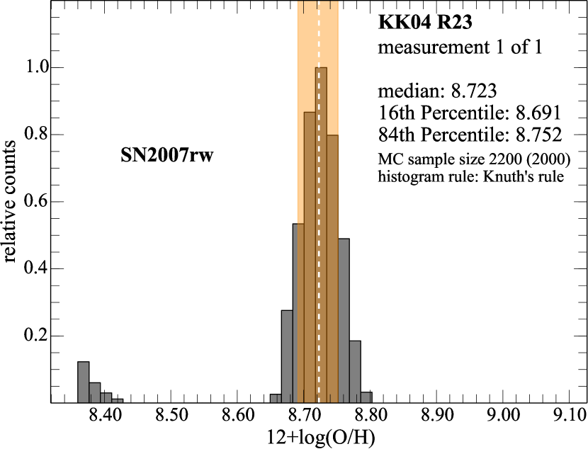
Since the metallicity distributions are not Gaussian, the percentiles we report cannot be expressed in terms of $\sigma$ values. In determining the confidence region for asymmetric and multi-modal distributions, there are broadly three approaches (Andrae 2010): choosing a symmetric interval, the shortest interval, or a central interval. With the central method, we determine the confidence interval by choosing the left and right boundaries such that the region outside the confidence interval on each side contains $16\%$ of the total distribution $-$ in analogy to the one-sigma-interval of a Gaussian distribution. This ensures that the algorithm finds the proper boundaries even for asymmetric, non-Gaussian distributions, and in the case of multiple peaks (Figure 2). In summary, the output for the measured value corresponds to the fiftieth (50%) percentile (median), while the lower error bar corresponds to the 50^th-16^th percentile and the upper error bar corresponds to 84^th-50^th of the metallicity estimate distribution.

The distributions for the D02 calibrator include the uncertainty in the fit parameters: the oxygen abundance in this calibrator is generated as $12+\log_{10}(O/H)$ = $9.12~{}\pm 0.05+(0.73~{}\pm 0.10)\times\mathrm{[N~{}II]}/\mathrm{H}\alpha$ (Denicoló et al., 2002). The parameters of the fit are generated as the sum of the nominal parameters (9.12 and 0.73) and a Gaussian distributed random value centered on zero, and within a standard deviation of 0.05 and 0.10, respectively, in the above units. Similarly, the distributions for the M13 calibrators include the uncertainty in the fit parameters as stated in Marino et al. (2013): the oxygen abundance as a function of [N II]/$\mathrm{H}\alpha$  is parametrized as $12+\log_{10}(O/H)$ = $8.743~{}\pm 0.027+(0.462~{}\pm 0.024)\times\mathrm{N~{}II}/\mathrm{H}\alpha$, and as a function of $\frac{\mathrm{[O~{}III]/H}\beta}{\mathrm{[N~{}II]/H}\alpha}$ as $12+\log_{10}(O/H)$ = $8.533~{}\pm 0.012+(0.214~{}\pm 0.012)\times\frac{\mathrm{[O~{}III]/H}\beta}{\mathrm{[N~{}II]/H}\alpha}$.

We note again that our code does not output the systematic uncertainty of each calibrator, which, for example, is $\sim$0.15 dex for KD02. However, if all metallicity measurements are in the same calibrator and only relative comparisons are made, as recommended by a number of authors, then the systematic error has no impact.

4.3.1 Visual diagnostics to interpret the metallicity outputs

Table 2Example Data and their Uncertainties based on Data in Modjaz et al. (2011)

site	[O II] $\lambda$3727	$\mathrm{H}\beta$	[O III] $\lambda$4959	[O III] $\lambda$5007	[O I] $\lambda$6300	$\mathrm{H}\alpha$	[N II] $\lambda$6584	[S II] $\lambda$6717	[S II] $\lambda$6731
08D	1.842 (.053)	0.958 (.032)	NaN	0.302 (.029)	0.127 (.021)	4.746 (.026)	1.642 (.022)	0.941 (.021)	0.543 (.019)
06fo	2.875 (.101)	1.251 (.044)	0.168 (.028)	0.064 (.025)	NaN	4.026 (.069)	0.781 (.033)	0.821 (.035)	0.573 (.032)

In order for the user to check the validity of a measurement, and to better understand the distribution of metallicity values, we provide two visualizations: for each set of input line fluxes, we generate a histogram of the output distribution in all metallicity calibrators calculated (Figure 1, 2, and 3), and for each set of input line fluxes we generate a box-and-whiskers plot (hereafter boxplot, for short) summarizing the result of all calibrators calculated (Figure 4). All the plots generated are created with Python matplotlib (Hunter, 2007).

Choosing the binning size for a histogram is not a trivial task. Hogg (2008), and Ivezić et al. (2014), among others, describes various data analysis recipes for selecting a histogram bin size. Too many bins will result in an “over-fit” histogram (showing structure that is in fact not in the distribution, thus perhaps decreasing the confidence in the metallicity measurement), while too few bins may miss features of the distribution (with the opposite effect). We provide several methods to generate the histograms, in order to enable the best possible visualization, given the computational power, for visual interpretation. However, we emphasize that our metallicity and confidence interval calculation is robust to this choice, since it calculates the percentiles of the unbinned distribution.

By default, we use Knuth’s method to choose the number of bins $N_{\mathrm{bins}}$ for each histogram. Knuth’s method optimizes a Bayesian fitness function across fixed-width bins (Knuth, 2006). Additionally, we enable a number of binning options from which the user can choose, including: the square root of the number of points, $N_{\mathrm{bins}}=\sqrt{N}$, Rice rule ($N_{\mathrm{bins}}~{}=~{}2\sqrt[3]{N}$, e.g., Hastie et al. 2009), Doane’s formula ($N_{\mathrm{bins}}~{}=~{}1+\mathrm{log}_{2}{N}+\mathrm{log}_{2}\left(1+\mathrm{Kurt}\sqrt{(N/6)}\right)$, where Kurt is the third moment of the distribution, Doane 1976), and the full Bayesian solution, known as Bayesian Blocks, which optimizes a fitness function across an arbitrary configuration of bins, such that the bins are of variable size (Scargle et al., 2013). The implementation of the latter method requires the astroML Python package to be installed on the user’s system (Vanderplas et al. 2012). If the astroML package is not found, the code will default to Knuth’s method. As mentioned, Knuth’s method implies an optimization. In cases in which the convergence takes too long, or if the number of bins after the minimization is $N_{\mathrm{bins}}/\sqrt{N}>5$ or $N_{\mathrm{bins}}/\sqrt{N}<1/3$, the code will revert to Rice rule. Some methods may be computationally prohibitive with a very large sample size, or very little computational power, such as the Bayesian methods that rely on optimization (Knuth’s method and the Bayesian Block method) in which case it may be convenient for a user to choose Doane’s formula, Rice rule, or even the square root of the number of samples.

Figure 3.— The Kernel Density for the distribution of values for the KD02comb calibrator for the first measurement of our example data (Table 2). The Kernel Density is displayed as a blue shaded region, and is calculated via KD Tree with a Gaussian kernel with bandwidth given by Silverman’s rule, and normalized, as described in subsubsection 4.3.1. The histogram of the distribution with bin size chosen according to Knuth’s method is also plotted (gray bins) and the median and confidence intervals are shown as described in Figure 1.

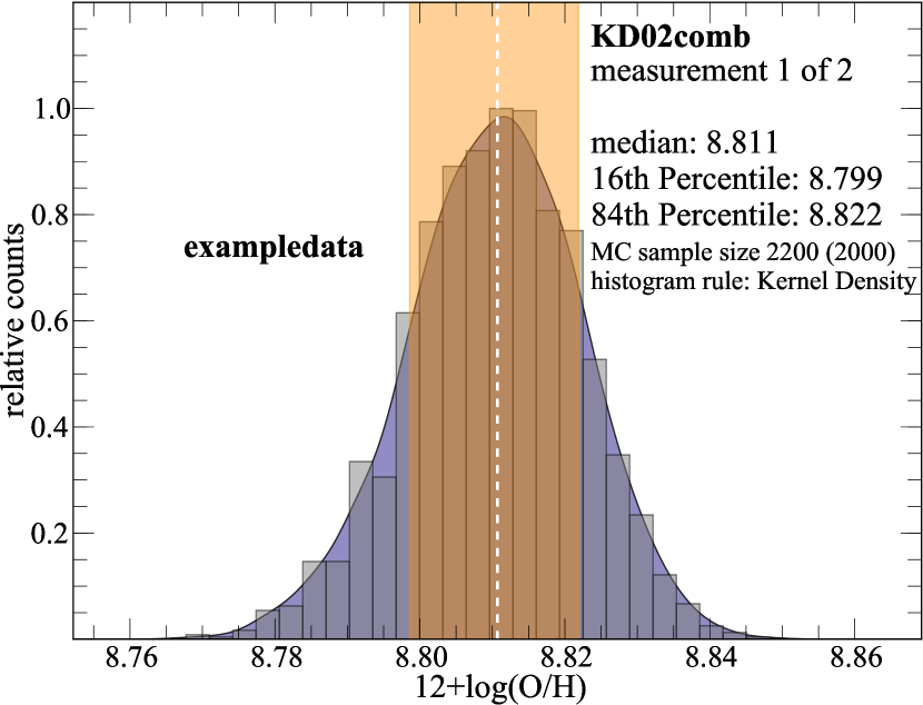
Lastly, the user can generate and visualize the metallicity distribution Kernel Density if the sklearn package is installed. Kernel Density Estimation (KDE) alleviates the problem of choosing the bin size, at the cost of specifying a convolution kernel. The Kernel Density of the distribution is here calculated via KD Tree with a gaussian kernel, as explained in the sklearn package documentation. The bandwidth of the kernel is chosen according to Silverman’s rule (Silverman, 1986). The results will then show both a histogram, with $N_{\mathrm{bins}}$ chosen via Knuth’s method, as well as the distribution Kernel Density, as shown in Figure 3. The KDE is saved as a binary python object (an sklearn KernelDensity object), so that it can be recovered outside the code and used as a probability distribution for further inference.

The histograms are always normalized so that the highest bin value is 1, and the Kernel Density is normalized to contain the same area as the overplotted histogram.

Figure 4.— A box-and-whiskers plot showing the comparison of the results of nine metallicity calculations, corresponding to five calibrators as listed above, calculated from the same set of measured lines (Table 2, host galaxy of SN 2008D). For each calibrator, the median of the resulting distribution is plotted as a horizontal line, the interquartile range (IQR) is represented as an orange box, and the bars, joined to each end of the box by a dashed line, represent the minimum and maximum of the distribution excluding outliers, where outliers are defined as any point farther than $1.5\times$ IQR from the edges for the IQR. A range of values for Solar oxygen abundance that are commonly found in the literature is shown as a gray horizontal band.

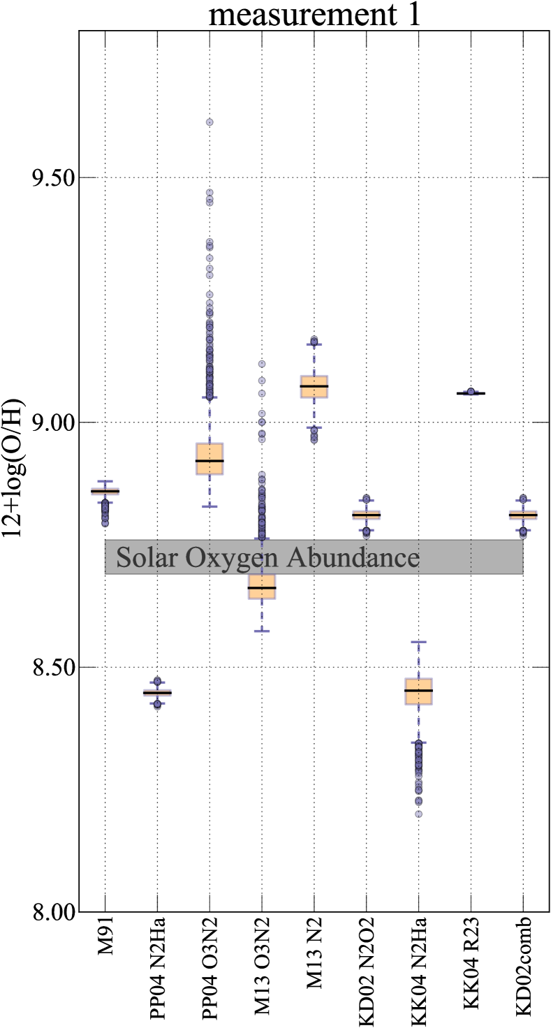
At each run the code also generates a boxplot (Figure 4) that summarizes the result from each calibrator the user chooses to calculate. For each calibrator, the median of the $12+\log_{10}(O/H)$  distribution is plotted as a black horizontal line. The height of the corresponding box represents the $25^{th}$ percentile of the $12+\log_{10}(O/H)$  distribution, known as the interquartile range (IQR). The bars represent the maximum and minimum value of the distribution, excluding outliers. The outliers are plotted as circles, and are defined as all data points farther than $1.5\times\mathrm{IQR}$ from the $25^{th}$ percentile (i.e. from either end of the box).

The Solar oxygen abundance is indicated in this plot for comparison: a gray box shows a range of estimated values for Solar oxygen abundances, from $12+\log_{10}(O/H)$=8.69 (Asplund et al., 2009) to $12+\log_{10}(O/H)$=8.76 (Caffau et al., 2011). The diagnostics requested by the user have a slot in the plot (in the example in Figure 3 the computed calibrators are the PP04, the M13, and the KD02 calibrators), as do diagnostics that are computed in support of other requested diagnostics (M91 in this case, which is needed to calculate KD02_comb). However a slot exists in the plot whether the diagnostic can be produced or not, i.e. if the set of input lines does not allow a requested calibrator to be calculated an empty column will be generated in this plot.

With this plot, the user can immediately check for consistency or scatter in the metallicities derived by the requested calibrators (e.g., there are well-known systematic offsets between different methods, where the $T_{e}$-based, empirical methods usually give lower values than the photoionization based ones), and coarsely assess the shape of the distribution in each calibrator (e.g. strong asymmetry or bimodality would show up as an asymmetric box, or a very asymmetric distribution of outliers). Although, as we stated earlier, relative comparison within a metallicity calibrator are valid despite the typical spread in metallicity derived by different strong line methods, a particularly large spread may indicate difficulties in assessing metallicity for this spectrum. The user is responsible for understanding the strengths and caveats of the various diagnostics and in which ranges and conditions they may be used. The visualization tools we provide are meant to help the user understand the reliability of the strong-line metallicity derived for a particular HII region.

4.4. Visual diagnostic to assure completeness of the MC simulation

Figure 5.— Cumulative plots of the distribution of metallicity values for the D02 (Denicoló et al., 2002) and KD02 calibrator (Kewley & Dopita 2002, as updated by Kewley & Ellison 2008), chosen here just as examples, where $x$ indicates $12+\log_{10}(O/H)$. The input data is “example data 1”, the emission line values for the host galaxy of SN 2008D from Modjaz et al. (2011). This plot provides a visual diagnostic of sample completeness. In each plot the cumulative distribution of metallicity values is shown for randomly chosen subsamples of 10%, of 25%, 50%, and 75% of the data, and for all data in the distribution. In the left top and bottom plots, the distributions are generated from an $N=200$ sample, in the center plots from an $N=2,000$, and in the right-most column from an $N=20,000$ samples. The increasing overlap of the distributions reflects increasing completeness. In the left plots, the distributions do not fully overlap, indicating that completeness is not achieved with the $N=200$ sample. On the other end, since all subsamples are indistinguishable in the rightmost top and bottom plots, from an $N=20,000$ sample, we conclude that completeness is already achieved at the smallest subsample in the plots on the right, 10% of the $N=20,000$ sample, for our example data. That is, $N=2,000$ is a sufficiently large sample for these data, and these diagnostics.

The user chooses $N$, the number of samples to be generated. The sample size is automatically increased by 10% at the beginning of the run, in order to assure that even if during the calculations some of the output metallicities were to result in non-valid values (NaN’s or infinities, for example, if divisions by very small numbers are required) the actual sample size is at least as large as the user intended. The code rarely produces non-valid values, and if the size of the valid output distribution were in the end smaller than the requested value $N$ (if the number of non-valid outputs is larger than 0.1$N$), the user should worry about the reliability of the set of input line fluxes used.

The reliability of the metallicity estimates depends crucially on the sample size being sufficiently large to properly characterize the distribution of metallicity values. It is, however, not trivial to decide when $N$ is sufficiently large. As soon as $N$ is large enough, and the distribution is well characterized, increasing the synthetic sample size will not change its shape.

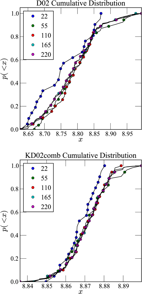
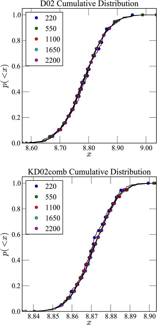
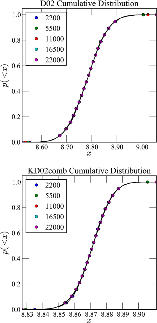
Let us consider a cumulative distribution for a metallicity calibrator: D02, for example, which has noise from the measurement errors, as well as from the error in the fit parameters, or KD02, which uses a non-linear combination of the input line flux values. We generate three distributions with $N=200$, $N=2,000$, and $N=20,000$ for both D02 and KD02comb. For each of these distributions we randomly select four subsamples of size 0.1$N$, 0.25$N$, 0.5$N$, and 0.75$N$, and we overplot the cumulative distribution of each subsample to that of the full sample. If all subsamples, including the smallest one (0.1$N$) constituted a sufficiently large MC sample to properly characterize the underlying distribution, all these cumulative distribution would typically appear smooth and, most importantly, they would overlap.

In Figure 5 we show these cumulative plots for a distribution generated with $N=200$, $N=2,000$, and $N=20,000$ for D02 and KD02comb. The cumulative distributions for the subsets of the $N=200$ samples simulation (left panel in Figure 5) are noisy and rather different from each other, indicating that 200 data points are not a sufficiently large dataset. Conversely, at $N=20,000$ (right panel) the distributions are indistinguishable, indicating that a sample of size $N=2,000$ (=0.1$N$) is already large enough to fully describe the distribution. The $N=2,000$ cumulative distributions rapidly converge as the subsample size increases, indicating that a value of $N$ between 200 and 2,000 samples will characterize the distribution appropriately for our example dataset. In light of this we choose, conservatively, $N=2,000$ to run our simulations for this dataset.

The appropriate number $N$ of samples will depend on the calibrator calculated and on the input data. The errors on the measurements and the calculations performed to derive the metallicity from line ratios, which for many calibrators are non-linear, will determine the shape of the distribution, and thus the number of data points that are needed to fully characterize it. Consult the repository README for instructions on how to generate these diagnostic plots.

4.5. Performance and Benchmarks

We ran a benchmark calculation on a MacBook Air with a dual-core Intel Core i7 (1.7 GHz) and 8GB of 1600 MHz DDR3 memory. The dataset we used for the calculation includes two sets of line measurements (measurement 1, the host galaxy of SN 2008D, and measurement 2, the host galaxy of SN 2006fo). The flux values and their associated errors are shown in Table 2. The code performs simple algebraic operations on large data arrays. It is vectorized along the sample-size dimension, so that the code loops over the smaller dimension corresponding to the number of sets of line measurements in input (two in our example data), while operations are generally performed on the $N$-dimensional vectors storing the synthetic measurements, and the $N$-dimensional variables derived from them (certain calibrators, such as KD02 and KK04, derive the ionization parameter in an iterative fashion, and require further loops).

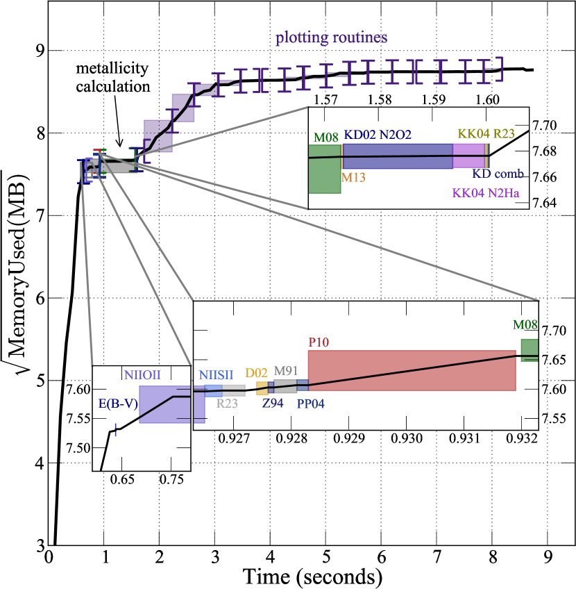
With full graphic output (all histograms are plotted) and performing all default metallicity calculations, except those of D13 (pyqz), for our example datasets and a sample size $N=2,000$ the time required by the code is $\sim 9$ seconds (wall clock time, and less than half a second longer in total CPU time, as the machine we tested on is dual-core), and less than 0.3 seconds of CPU time spent in the kernel within the process. Including the calibrators of D13 pyqz for the same datasets, the run time becomes $\sim 19$ seconds of clock time (and actual CPU time). The code time was tested on sets of 1, 2, 5, 10, 25, 50, and 100 identical measurements (copies of the emission line fluxes of the SN 2008D host galaxy in our example dataset) and the clock time is found to scale roughly quadratically with the number $m$ of measurement in input, but with a small quadratic coefficient: $t~{}\sim~{}7m+0.07m^{2}$. This means effectively that the 100 measurements sample will take 200 times longer than the 1 measurement sample (of course with dependence on which line values are available in each measurement, enabling different metallicity calibrators to be calculated). For the CPU time spent in the kernel we find a roughly linear relation with the number of input measurements, with a very shallow dependency: $t~{}\sim~{}0.05m$. This is the actual computational time in calculations performed in the code: most clock time is in fact spent in root finding, input-output, and plotting activities.

The time spent on plotting functions, which includes the calculation of the appropriate number of bins for each calibrator, is substantial: 1.67 seconds per distribution on average with 14 calls for this dataset (one for each metallicity calibrator, E(B-V), and $R_{23}$). We summarize the run time spent on each metallicity calibrator and memory usage for the host galaxy of SN 2008D, the first measurement of the sample dataset, in Figure 6. While the CPU usage is modest, the memory usage can be large, depending on the size of the sample. The memory usage ramps up quickly, as soon as the $N$ line samples are created, and remains fairly constant throughout the run. Figure 6 shows the memory used by each function in the code as a function of time for a single set of input lines of our example data (the host galaxy of SN 2008D). The calibrators that take longer are those that require root finding (e.g. M08), or optimizations (which are done iteratively, e.g. KD02_N2O2).

Figure 6.— Memory usage: we plot the square root of the memory usage in Megabytes as a function of time for running our code (using $N$=2,000 and all default metallicity calibrators except the D13 pyqz ones, and PP04) on a single set of measured emission lines (Table 2, host galaxy of SN 2008D). The square root is plotted, instead of the natural value, to enhance visibility. Three inserts show the regions where most of the metallicity calibrators are calculated, zoomed in, since the run time of the code is dominated by plotting routines, including the calculation of the bin size with Knuth’s rule. Each function call is represented by an opening and closing bracket in the main plot, and by a shaded rectangle in the zoomed-in insets. The calculation of $N2O2$, which requires 0.25 seconds, is split between two insets, as well as the calculation of the M08 calibrators (three calibrators) which require 0.65 seconds. Altogether, the calculation of metallicity in all default calibrators, except the D13 pyqz calibrators, takes $\sim 1$ seconds. For technical details about the D13 pyqz calibrators performance we refer the reader to the pyqz package.

The code is trivially parallelizable, as each measurement can be computed on a different core, and multiprocessing is enabled via the multiprocessing Python module. When multiprocessing is enabled, pyMCZit uses up to $n-1$ cores, where $n$ is the total number of available cores to the user, or less, if a smaller maximum number of cores is set by the user via the global variable MAXPROCESSES.

5. Comparison to prior uncertainty computation and other works

We compare our method with the results that appear in Modjaz et al. 2011 for 19 SN galaxies. We choose a SN host sample for our comparison, since investigations of the environments of extra-galactic transients, where observational errors dominate, are the studies that can benefit most from our implementation of metallicity calculations. We compare our results with the results that appeared in Modjaz et al. 2011 since for those results we have both all flux values in input and their errors, and the metallicities and uncertainties obtained in output. We note that this work includes only three calibrators: M91, PP04_O3N2, and KD02comb; however these calibrators cover the case of calibrators that are fully linear, that rely on decision trees, and mixed calibrators. We stress again that the PP04 calibrators are superseded by the M13 ones, but they can be used in this comparison nonetheless. Since our work is the implementation of existing calculations, it is beyond the scope of this paper to include a complete comparison of all calibrators: that burden was on the original authors and we refer the reader to the papers that present each method for that.

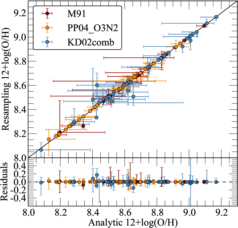
A previous method for determining the uncertainty in the oxygen abundance, used in Modjaz et al. 2011 as well as, for example in Modjaz et al. 2008; Kewley et al. 2010; Rupke et al. 2010 was an analytic approach, where the emission-line flux uncertainties are propagated into a measurement “envelope”: it found the extreme abundances obtained from the input fluxes minimizing (maximizing) the indicators used in the calculations by adding (subtracting) to the measured line flux values their uncertainties, thus producing envelope values for the metallicity. For comparison, we computed the metallicities and their errors in both ways (analytically and using our current MC sampling method) for three representative calibrators. We plot our results and the residuals in Figure 7. The errorbars in the residuals are generated by adding asymmetric errors in quadrature: $\mathrm{residual}_{\rm min}=\sqrt{x_{\rm max}^{2}+y_{\rm min}^{2}}$ and $\mathrm{residual}_{\rm max}=\sqrt{x_{\rm min}^{2}+y_{\rm max}^{2}}$.

This figure highlights a number of important points:

• The metallicity reported as the $50^{th}$ percentile of the metallicity parameter distribution from the MC sampling method is consistent with the analytically derived metallicity. The mean of the residuals is $\sim-2\times 10^{-3}$, $\sim 5\times 10^{-3}$, and $~{}\sim 5\times 10^{-2}$, for M91, PP04_O3N2, and KD02_comb respectively, for 20, 32, and 35 valid measurement from the Modjaz et al. (2011) data; the standard deviation of the residuals is $\sim 0.018,~{}0.005,~{}0.004$ respectively – well within the respective error bars - and thus, the published results still stand (unsurprisingly, since our code, aside for the calculation of the confidence interval, uses for these calibrators the same algorithms developed for IDLKD02).

• The MC sampling method has smaller error bars than the analytic method. This is easily understandable, since the analytic method assumes the worst-case-scenarios, as it basically yields two metallicity parameter draws (the “minimum” and “maximum”) which are in the tail of the full metallicity probability distribution. The MC sampling method empirically characterizes the full parameter estimation distribution.

The (minimal and statistically not significant) differences between our and the IDLKD02 implementation of the KD02_comb calibrator arise from numerical differences in the solutions of the root finding algorithms, and in the optimizations, which we carry out until convergence, while IDLKD02 estimated three iterations would be sufficient for minimization. The differences in the M91 and PP04_O3O2 calibrators are only due to the shape of the distributions.

Figure 7.— Comparison of metallicity estimation between the analytic method and our MC sampling method (top) and their residuals (bottom) for three different metallicity calibrators. Flux measurements come from 19 galaxies previously measured in Modjaz et al. (2011). Note that for KD02_comb and M91, and in most cases for PP04_O3N2 as well, the MC sampling error bars are smaller than those of the analytic propagation, which assumes worst-case scenarios. The metallicity value derived by our code, which is the 50th percentile of the metallicity distribution from MC sampling, is consistent with the analytically derived metallicity in all calibrators, for all measurements.

5.1. Comparison with other works

The field of SN host metallicity studies is rapidly developing, and these studies are crucial avenues for constraining the progenitor systems of different kinds of explosions. However, some the works in this field do not compute errors in the derived metallicities, and others do not show how they compute their statistical errors (e.g., Anderson et al. 2010; Leloudas et al. 2011; Sanders et al. 2012; Leloudas et al. 2014).

In contrast, the general metallicity field has considered in detail how to estimate the uncertainties in measured metallicities. However, when the codes are designed for local Galaxy metallicity measurements, they neglect the observational uncertainties, since they are negligible compared to other sources of error. Other codes are not open-source, and many of them are for specific calibrators. For example: Moustakas et al. (2010) also use MC sampling to estimate the metallicity uncertainties (in their case using $N$=500 trials and assuming a Gaussian distribution for metallicity parameter distribution) but only do this for two calibrators, KK04 and P05.

Some strong line methods fit a set of stellar population synthesis and photoionization models directly to the spectra of HII regions by changing the model parameters. For computing the metallicities of the SDSS star forming galaxies, Tremonti et al. (2004) fit a combination of stellar population synthesis models and photoionization models to the observed strong emission lines [O II], $\mathrm{H}\beta$, [O III], $\mathrm{H}\alpha$, [N II] and [S II] and report the median of the metallicity likelihood distribution as the metallicity estimate, with the width of the distribution giving the 1-$\sigma$ (Gaussian) error. Blanc et al. (2015) use Bayesian inference to derive the joint and marginalized posterior probability density functions for metallicity $Z$ and ionization parameter $q$ given a set of observed line fluxes and an input photoionization model. They provide a publicly available IDL implementation of their method named $IZI$ (inferring metallicities – $Z$ – and ionization parameters).

6. Conclusions

We have presented the open-source Python code pyMCZ that determines oxygen abundance and its error distribution from strong emission lines in a total of up to 15 diagnostics, 11 default and 4 additional upon request, where by diagnostic we intend a suite of metallicity calibrators that are published in a single article, and for a total of up to 32 different metallicity calibrators (since a number of diagnostics produce different metallicity estimates based on different input indicators). These estimates are based on the original KD02IDL code in KD02, and updated in KE08, and expanded to include more recently developed calibrators, and to generate confidence intervals for each calibrator via MC sampling. We supply visualization tools that, as part of the default output of pyMCZ, enable the user to assess the validity of each derived metallicity distribution and understand when line flux measurements may lead to misleading metallicity estimates, for example in proximity of the demarcation between the upper and lower branch for $R_{23}$-based methods. pyMCZ outputs the full estimated metallicity distribution (on demand), and its Kernel Density, and it offers visualization tools to assess the spread of the oxygen abundance in the different calibrators.

The validity of our metallicity measurements and of their confidence regions hinges upon generating probability distributions that properly sample the metallicity distribution, given the input parameters and the specific metallicity calculation algorithm. Thus, we have developed metrics that allow the user to ascertain that the sample drawn in the simulation is sufficiently large. However, we note that our code does not take into account systematic errors, but only computes the statistical ones.

This code is open access and we welcome input and further development from the community. Since the code is open-source, the users can include other metallicity calibrators and modify any parts of the algorithms, or any assumption (e.g. that the line flux errors are Gaussian distributed).

We hope that this open-access code will be helpful for the many different fields where gas-phase metallicities are important, and observational uncertainty are important in the error budget, including in the emerging field of SN and GRB host galaxies.

References

- Allen et al. (2008) Allen, M. G., Groves, B. A., Dopita, M. A., Sutherland, R. S., & Kewley, L. J. 2008, ApJS, 178, 20
- Alloin et al. (1979) Alloin, D., Collin-Souffrin, S., Joly, M., & Vigroux, L. 1979, A&A, 78, 200
- Anderson et al. (2010) Anderson, J. P., Covarrubias, R. A., James, P. A., Hamuy, M., & Habergham, S. M. 2010, MNRAS, 407, 2660
- Andrae (2010) Andrae, R. 2010, ArXiv e-prints, arXiv:1009.2755
- Asplund et al. (2009) Asplund, M., Grevesse, N., Sauval, A. J., & Scott, P. 2009, ARA&A, 47, 481
- Baldwin et al. (1981) Baldwin, J. A., Phillips, M. M., & Terlevich, R. 1981, PASP, 93, 5
- Berg et al. (2015) Berg, D. A., Croxall, K. V., Skillman, E. D., et al. 2015, ApJ, 808, 42.
- Blanc et al. (2015) Blanc, G. A., Kewley, L., Vogt, F. P. A., & Dopita, M. A. 2015, ApJ, 798, 99
- Bonate (2011) Bonate, P. 2011, Pharmacokinetic-Pharmacodynamic Modeling and Simulation, SpringerLink : Bücher (Springer)
- Bruzual A. & Charlot (1993) Bruzual A., G., & Charlot, S. 1993, ApJ, 405, 538
- Bundy et al. (2015) Bundy, K., Bershady, M. A., Law, D. R., et al. 2015, ApJ, 798, 7
- Caffau et al. (2011) Caffau, E., Ludwig, H.-G., Steffen, M., Freytag, B., & Bonifacio, P. 2011, Sol. Phys., 268, 255
- Cardelli et al. (1989) Cardelli, J. A., Clayton, G. C., & Mathis, J. S. 1989, ApJ, 345, 245
- Charlot & Longhetti (2001) Charlot, S., & Longhetti, M. 2001, MNRAS, 323, 887
- Cid Fernandes et al. (2010) Cid Fernandes, R., Stasińska, G., Schlickmann, M. S., et al. 2010, MNRAS, 403, 1036
- Denicoló et al. (2002) Denicoló, G., Terlevich, R., & Terlevich, E. 2002, MNRAS, 330, 69
- Díaz & Pérez-Montero (2000) Díaz, A. I., & Pérez-Montero, E. 2000, MNRAS, 312, 130
- Doane (1976) Doane, D. P. 1976, The American Statistician, 30, 181
- Dopita & Evans (1986) Dopita, M. A., & Evans, I. N. 1986, ApJ, 307, 431
- Dopita et al. (2013) Dopita, M. A., Sutherland, R. S., Nicholls, D. C., Kewley, L. J., & Vogt, F. P. A. 2013, ApJS, 208, 10
- Efron (1979) Efron, R. 1979, Ann. Stat., 7, 1
- Evans & Dopita (1985) Evans, I. N., & Dopita, M. A. 1985, ApJS, 58, 125
- Ferland et al. (1998) Ferland, G. J., Korista, K. T., Verner, D. A., et al. 1998, PASP, 110, 761
- Grevesse et al. (2010) Grevesse, N., Asplund, M., Sauval, A. J., & Scott, P. 2010, Ap&SS, 328, 179
- Hastie et al. (2009) Hastie, T., Tibshirani, R., & Friedman, J. 2009, The Elements of Statistical Learning: Data Mining, Inference, and Prediction (Springer Science+Business Media, New York)
- Hogg (2008) Hogg, D. W. 2008, ArXiv e-prints, arXiv:0807.4820
- Hunter (2007) Hunter, J. D. 2007, Computing In Science & Engineering, 9, 90
- Ivezić et al. (2014) Ivezić, Ž., Connolly, A., Vanderplas, J., & Gray, A. 2014, Statistics, Data Mining and Machine Learning in Astronomy (Princeton University Press)
- Johnson & Li (2012) Johnson, J. L., & Li, H. 2012, ApJ, 751, 81
- Kauffmann et al. (2003) Kauffmann, G., Heckman, T. M., Tremonti, C., et al. 2003, MNRAS, 346, 1055
- Kelly & Kirshner (2012) Kelly, P. L., & Kirshner, R. P. 2012, ApJ, 759, 107
- Kewley & Dopita (2002) Kewley, L. J., & Dopita, M. A. 2002, ApJS, 142, 35
- Kewley & Ellison (2008) Kewley, L. J., & Ellison, S. L. 2008, ApJ, 681, 1183
- Kewley et al. (2006) Kewley, L. J., Groves, B., Kauffmann, G., & Heckman, T. 2006, MNRAS, 372, 961
- Kewley et al. (2010) Kewley, L. J., Rupke, D., Zahid, H. J., Geller, M. J., & Barton, E. J. 2010, ApJ, 721, L48
- Knuth (2006) Knuth, K. H. 2006, ArXiv Physics e-prints, physics/0605197
- Kobulnicky & Kewley (2004) Kobulnicky, H. A., & Kewley, L. J. 2004, ApJ, 617, 240
- Leloudas et al. (2011) Leloudas, G., Gallazzi, A., Sollerman, J., et al. 2011, A&A, 530, A95
- Leloudas et al. (2014) Leloudas, G., Schulze, S., Kruehler, T., et al. 2015, MNRAS, 449, 917L.
- Levesque et al. (2010) Levesque, E. M., Berger, E., Kewley, L. J., & Bagley, M. M. 2010, AJ, 139, 694
- López-Sánchez et al. (2012) López-Sánchez, Á. R., Dopita, M. A., Kewley, L. J., et al. 2012, MNRAS, 426, 2630
- Lunnan et al. (2014) Lunnan, R., Chornock, R., Berger, E., et al. 2014, ApJ, 787, 138
- Maiolino et al. (2008) Maiolino, R., Nagao, T., Grazian, A., et al. 2008, A&A, 488, 463
- Marino et al. (2013) Marino, R. A., Rosales-Ortega, F. F., Sánchez, S. F., et al. 2013, A&A, 559, A114
- McGaugh (1991) McGaugh, S. S. 1991, ApJ, 380, 140
- Mendoza & Bautista (2014) Mendoza, C., & Bautista, M. A. 2014, The Astrophysical Journal, 785, 91
- Modjaz (2012) Modjaz, M. 2012, in IAU Symposium, Vol. 279, IAU Symposium, 207–211
- Modjaz et al. (2011) Modjaz, M., Kewley, L., Bloom, J. S., et al. 2011, ApJ, 731, L4
- Modjaz et al. (2008) Modjaz, M., Kewley, L., Kirshner, R. P., et al. 2008, AJ, 135, 1136
- Mollá et al. (2009) Mollá, M., García-Vargas, M. L., & Bressan, A. 2009, MNRAS, 398, 451
- Moustakas et al. (2010) Moustakas, J., Kennicutt, Jr., R. C., Tremonti, C. A., et al. 2010, ApJS, 190, 233
- Nicholls et al. (2012) Nicholls, D. C., Dopita, M. A., & Sutherland, R. S. 2012, ApJ, 752, 148
- Osterbrock (1989) Osterbrock, D. E. 1989, Astrophysics of Gaseous Nebulae and Active Galaxies (Mill Vallery: University Science Books)
- Owocki & Scudder (1983) Owocki, S. P., & Scudder, J. D. 1983, ApJ, 270, 758
- Pagel et al. (1979) Pagel, B. E. J., Edmunds, M. G., Blackwell, D. E., Chun, M. S., & Smith, G. 1979, MNRAS, 189, 95
- Pan et al. (2014) Pan, Y.-C., Sullivan, M., Maguire, K., et al. 2014, MNRAS, 438, 1391
- Peimbert (1967) Peimbert, M. 1967, ApJ, 150, 825
- Pérez-Montero (2014) Pérez-Montero, E. 2014, MNRAS, 441, 2663
- Pettini & Pagel (2004) Pettini, M., & Pagel, B. E. J. 2004, MNRAS, 348, L59
- Pilyugin (2001) Pilyugin, L. S. 2001, A&A, 369, 594
- Pilyugin & Thuan (2005) Pilyugin, L. S., & Thuan, T. X. 2005, ApJ, 631, 231
- Pilyugin et al. (2012) Pilyugin, L. S., Vílchez, J. M., Mattsson, L., & Thuan, T. X. 2012, MNRAS, 421, 1624
- Pilyugin et al. (2010) Pilyugin, L. S., Vílchez, J. M., & Thuan, T. X. 2010, ApJ, 720, 1738
- Rupke et al. (2010) Rupke, D. S. N., Kewley, L. J., & Chien, L.-H. 2010, ApJ, 723, 1255
- Sánchez et al. (2012) Sánchez, S. F., Kennicutt, R. C., Gil de Paz, A., et al. 2012, A&A, 538, A8
- Sánchez et al. (2015) Sánchez, S. F., Pérez, E., Rosales-Ortega, F. F., et al. 2015, A&A, 574, A47
- Sanders et al. (2012) Sanders, N. E., Soderberg, A. M., Levesque, E. M., et al. 2012, ApJ, 758, 132
- Scargle et al. (2013) Scargle, J. D., Norris, J. P., Jackson, B., & Chiang, J. 2013, ApJ, 764, 167
- Silverman (1986) Silverman, B. W. 1986, Density Estimation for Statistics and Data Analysis (Chapman and Hall)
- Simón-Díaz & Stasińska (2011) Simón-Díaz, S., & Stasińska, G. 2011, A&A, 526, A48+
- Stasińska (2002) Stasińska, G. 2002, ArXiv Astrophysics e-prints, astro-ph/0207500
- Stasińska (2010) Stasińska, G. 2010, in IAU Symposium, Vol. 262, IAU Symposium, ed. G. R. Bruzual & S. Charlot, 93–96
- Tremonti et al. (2004) Tremonti, C. A., Heckman, T. M., Kauffmann, G., et al. 2004, ApJ, 613, 898
- Vanderplas et al. (2012) Vanderplas, J., Connolly, A., Ivezić, Ž., & Gray, A. 2012, in Conference on Intelligent Data Understanding (CIDU), 47 –54
- Vasyliunas (1968) Vasyliunas, V. M. 1968, J. Geophys. Res., 73, 5810
- Zaritsky et al. (1994) Zaritsky, D., Kennicutt, Jr., R. C., & Huchra, J. P. 1994, ApJ, 420, 87