Numerical testing in determination of sound speed from a part of boundary by the BC-method

Abstract

We present the results of numerical testing on determination of the sound speed $c$ in the acoustic equation $u_{tt}-c^{2}\Delta u=0$ by the boundary control method. The inverse data is a response operator (a hyperbolic Dirichlet-to-Neumann map) given on controls, which are supported on a part of the boundary. The speed is determined in the subdomain covered by acoustic rays, which are emanated from the points of this part orthogonally to the boundary. The determination is time-optimal: the longer is the observation time, the larger is the subdomain, in which $c$ is recovered. The numerical results are preceded with brief exposition of the relevant variant of the BC-method.

Key words:  acoustic equation, time-domain inverse problem, determination from part of boundary, boundary control method.

MSC:  35R30, 65M32, 86A22.

1 Introduction

1.1 About the method

The boundary control method (BCM) is an approach to inverse problems based on their relations with control and system theory [5, 7, 14]. It is a rigorously justified mathematical method of synthetic character: Riemannian geometry, asymptotic methods in PDE, functional analysis and operator theory are in the use. Beginning on its foundation in 1986 [4], there was a question whether such a purely theoretical method is available for numerical implementation. The first affirmative results were obtained by V.B.Filippov in two-dimensional problem of the density $\rho=c^{-2}$ determination via the spectral inverse data [12]. Later on, an algorithm based on the spectral variant of the BCM was elaborated and tested by S.A.Ivanov and V.Yu.Gotlib in [11, 7].

A dynamical variant of the BCM deals with time-domain inverse data that is a response operator (hyperbolic Dirichlet-to-Neumann map). It provides time-optimal reconstruction: the longer is the observation time, the bigger is the subdomain, in which the parameters are recovered. It is the feature, which makes this variant most relevant for possible applications to acoustics and geophysics. The corresponding algorithm was elaborated and tested by V.Yu.Gotlib in [10]. It recovers the density in a near-boundary layer from the data given on the whole boundary.

Time-optimal determination of density via the spectral and time-domain inverse data given on a part of boundary is proposed in [5]. The procedure uses singular harmonic functions; its spectral variant was realized numerically (see [5], section 7.7). In [6] and [8], its dynamical variant was modified to make it more prospective for applications in geophysics, the modification being based on geometrical optics.

In beginning of 2000’s, L.Pestov proposed a version of the BCM, which determines some intrinsic bilinear forms containing parameters under reconstruction via the inverse data and, then, recovers the parameters from the forms. This version is not time-optimal but, on expense of big enough observation time, provides more stable numerical algorithms. The results of the collaboration, which develops this approach in the I.Kant Baltic Federal University (Kaliningrad, Russia), are presented in [19, 20, 21].

Recently, L.Oksanen applied the BCM for numerical reconstruction of the obstacle [18].

There also exists a time optimal and data optimal approach by V.Romanov [22] but it is not implemented and tested yet. Another (not optimal) direct reconstruction methods, which are numerically (and experimentally) tested, see in [3, 15, 16].

1.2 Inverse problem

The goal of our work is to elaborate the BC-algorithm for time-optimal determination of the sound speed via the time-domain inverse data given at a part of boundary, and test it in numerical experiment.

$\bullet$   Let $\Omega\subset{\mathbb{R}}^{n}$ be a (possibly, unbounded) domain with the boundary $\Gamma$. We deal with a dynamical system

$$u_{tt}-c^{2}\Delta u=0 {\text{in}}\,\,\Omega\times(0,T)$$ (1.1)

$$u|_{t=0}=u_{t}|_{t=0}=0 {\text{in}}\,\,{\overline{\Omega}}$$ (1.2)

$$u=f {\text{on}}\,\,\Gamma\times[0,T]\,,$$ (1.3)

where $c=c(x)$ is a smooth enough positive function (speed of sound), $f$ is a boundary control, $u=u^{f}(x,t)$ is a solution (wave). With the system one associates a response operator

$$R^{T}:\,f\mapsto u^{f}_{\nu}\big{|}_{\Gamma\times[0,T]}\,,$$ (1.4)

where $(...)_{\nu}$ is a derivative with respect to the outward normal $\nu$ on $\Gamma$. In a general form, the inverse problem is to answer the question: To what extent does the response operator determine the sound speed into the domain? Also, the determination procedures are of principal interest.

System (1.1)–(1.3) is hyperbolic and, as such, obeys the finiteness of the domains of influence (FDI). It describes the waves propagating with finite speed $c$, and the relevant setup of the inverse problem must take this property into account. Such a setup is given below, after geometric preliminaries.

$\bullet$  The sound speed induces a travel time metric $d\tau^{2}=c^{-2}|dx|^{2}$ (shortly, $c$-metric) and the corresponding distance $\tau(x,y)$ in $\Omega$. For a subset $A\subset\overline{\Omega}$, by

$$\Omega^{\xi}_{A}:=\{x\in\overline{\Omega}\,|\,\,\tau(x,A)<\xi\}$$

we denote its $c$-metric neighborhood of radius $\xi$.

By $r^{\xi}_{\gamma}$ we denote a geodesic in $c$-metric (ray), which is emanated from $\gamma\in\Gamma$ into $\Omega$ in direction $-\nu$, and is of the $c$-length $\xi$. Let $\sigma\subset\Gamma$ be a part of the boundary. A set

$$B^{T}_{\sigma}:=\bigcup_{\gamma\in\sigma}r^{T}_{\gamma}\subset\overline{\Omega^{T}_{\sigma}}$$

is called a ray tube. On Fig 1a,b, the neighborhood $\Omega^{T}_{\sigma}$ and tube $B^{T}_{\sigma}$ are contoured by the closed lines $\{1,2,3,4,5,6,1\}$ and $\{5,6,2,3,5\}$ respectively ($B^{T}_{\sigma}$ is shaded).

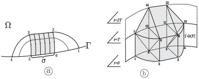
Figure 1: Tube $B^{T}$ and domain $D^{2T}_{\sigma}$

If $T$ is small enough then the ray field is regular in the tube. Let $T_{\sigma}$ be the infimum of $T$’s, for which such a regularity does occur.

Convention 1.

In what follows, unless otherwise specified, we assume that $\sigma$ is diffeomorphic to a disk $\{p\in{\mathbb{R}}^{n-1}\,|\,\,|p|\leq 1\}$ and $T<T_{\sigma}$. Such a case is said to be regular.

The part $\sigma$ determines the space-time domains

$$D^{2T}_{\sigma}:=\{(x,t)|\,x\in\Omega^{T}_{\sigma},\,0<\tau(x,\sigma)<2T-t\}\quad{\rm and}$$

$$E^{T}_{\sigma}:=\{(x,t)|\,x\in\Omega^{T}_{\sigma},\,0\leq t<\tau(x,\sigma)\},$$

and the space-time surfaces

$$\Theta^{T}_{\sigma}:=\overline{D^{2T}_{\sigma}}\cap\{\Gamma\times[0,T]\}\,,\quad\Theta^{2T}_{\sigma}:=\overline{D^{2T}_{\sigma}}\cap\{\Gamma\times[0,2T]\}.$$

All of them are mapped by the projection $(x,t)\mapsto x$ to $\overline{\Omega^{T}_{\sigma}}$. Domain $D^{2T}_{\sigma}$ is shown on Fig 1.b (shaded). Domain $E^{T}_{\sigma}\subset D^{2T}_{\sigma}$ lies under the surface $\{(x,t)\,|\,\,t=\tau(x,\sigma)\}$, which consists of three parts countered by the closed lines $\{6,7,8,6\}$, $\{5,6,8,9,5\}$, and $\{5,9,10,5\}$. The surfaces $\Theta^{2T}_{\sigma}$ and $\Theta^{T}_{\sigma}$ are countered by the lines $\{1,6,5,4,10,13,14,7,1\}$ and $\{1,6,5,4,10,11,12,7,1\}$ respectively.

If $c<c_{*}=\rm const$ holds in $\overline{\Omega}$ then for the sets

$$\sigma^{\xi}:=\{\gamma\in\Gamma\,|\,\,\tau(\gamma,\sigma)\leq\xi\}\quad{\rm and}\quad\sigma^{\xi}_{*}:=\{\gamma\in\Gamma\,|\,\,{\rm dist}_{{\mathbb{R}}^{n}}(\gamma,\sigma)\leq c_{*}\xi\}$$ (1.5)

one has $\sigma^{\xi}\subset\sigma^{\xi}_{*}$, and the relations

$$\Theta^{T}_{\sigma}\,=\,\sigma^{T}\times[0,T]\,\subset\,\sigma^{T}_{*}\times[0,T]$$ (1.6)

are valid.

$\bullet$  Assign a control $f$ to a class ${\cal F}^{2T}_{\sigma}$ if ${\rm supp\,}f\subset\sigma\times[0,2T]$, i.e., it acts from $\sigma$ during the time interval $0\leq t\leq 2T$. Owing to the FDI, an extension of system (1.1)–(1.3) of the form

$$u_{tt}-c^{2}\Delta u=0 {\text{in}}\,\,D^{2T}_{\sigma}$$ (1.7)

$$u=0 {\text{in}}\,\,E^{T}_{\sigma}$$ (1.8)

$$u=f\in{\cal F}^{2T}_{\sigma}$$ (1.9)

turns out to be a well-posed problem, its solution $u^{f}$ being determined by the values of the speed $c$ in the subdomain $\Omega^{T}_{\sigma}$ (does not depend on $c|_{\Omega\setminus\Omega^{T}_{\sigma}}$). The same is valid for the response operator

$$R^{2T}_{\sigma}:\,f\mapsto u^{f}_{\nu}\big{|}_{\Theta^{2T}_{\sigma}}$$ (1.10)

associated with this problem: it is also determined by $c|_{\Omega^{T}_{\sigma}}$.

By the latter, the relevant setup of the inverse problem is: for a fixed $T>0$, given the operator $R^{2T}_{\sigma}$ determine the speed $c$ in $\Omega^{T}_{\sigma}$.

The use of the doubled time $2T$ is quite natural by kinematic reasons. The subdomain $\Omega^{T}_{\sigma}$ is prospected with waves initiated at $\sigma$. To search the whole $\Omega^{T}_{\sigma}$, the waves have to fill it (that takes $T$ time units) and return back to the boundary (for the same time $T$) to be detected by the external observer, which implements measurements at $\Gamma$.

Convention 2.

The operator $R^{2T}_{\sigma}$ is introduced so that, for the times $0\leq t\leq T$ the images $R^{2T}_{\sigma}f$ are defined on the set $\Theta^{T}_{\sigma}$ only. For convenience of further formulations, we put $R^{2T}_{\sigma}f\big{|}_{0\leq t\leq T}$ to be extended from $\Theta^{T}_{\sigma}$ to $\Gamma\times[0,T]$ by zero.

1.3 Results and comments

$\bullet$  Let $\sigma\subset\Gamma$ and $T>0$ be given. Our a priori assumptions are that $T<T_{\sigma}$ (i.e., we deal with the regular case) and the sound speed upper bound $c_{*}$ is known. Under these assumptions, we propose a procedure, which recovers the speed $c$ in the tube $B^{T}_{\sigma}$ via the operator $R^{2T}_{\sigma}$. Then, we demonstrate the results of numerical testing of the algorithm based on this procedure.

$\bullet$   In fact, the procedure utilizes not the complete operator $R^{2T}_{\sigma}$ but some information, which it determines. Namely, as will be seen, to recover $c\big{|}_{\Omega^{T}_{\sigma}}$, it suffices for the external observer to possess the following options:

1. for any $f,g\in{\cal F}^{2T}_{\sigma}$ obeying the oddness condition

   $$f(\cdot,T)=-f(\cdot,2T-t),\quad g(\cdot,T)=-g(\cdot,2T-t)\,,\qquad 0\leq t\leq 2T\,,$$

   one can compute the integral

   $$I^{T}_{\sigma}[f,g]:=\int_{\sigma\times[0,2T]}u^{Jf}_{\nu}(\gamma,t)g(\gamma,t)\,d\Gamma dt=(R^{2T}_{\sigma}Jf,g)_{{\cal F}^{2T}_{\sigma}}\,,$$ (1.11)

   where $J:{\cal F}^{2T}_{\sigma}\to{\cal F}^{2T}_{\sigma}$ is an integration: $(Jf)(\cdot,t):=\int_{0}^{t}f(\cdot,s)\,ds$.

2. for any odd $f\in{\cal F}^{2T}_{\sigma}$, one can detect $u^{f}_{\nu}\big{|}_{\sigma^{T}_{*}\times[0,T]}=R^{2T}_{\sigma}f\big{|}_{\sigma^{T}_{*}\times[0,T]}$, i.e., implement the measurements on $\sigma^{T}_{*}$ (but not on the whole $\Gamma$!) during the time interval $[0,T]$ (but not $[0,2T]$!)

$\bullet$  In principle, the proposed procedure is identical to the versions [6] and [8]. Therefore, its exposition is short: we omit some proofs and derivations, referring the reader to the mentioned papers for detail. In the mean time, here we deal with more refined (rigorously time-optimal) data that is the operator $R^{2T}_{\sigma}$, in contrast to [6] and [8], where the operator $R^{2T}$ corresponding to system (1.1)–(1.3) with the final time $t=2T$, is used as the inverse data.

$\bullet$  One of the features and advantages of the BCM is that it reduces nonlinear inverse problems to linear ones. In particular, the main fragment of the algorithm, which recovers $c$, is the solving a big-size linear algebraic system. The matrix of the system is of the form $\{I^{T}_{\sigma}[f_{i},f_{j}]\}_{i,j=1}^{N}$ for a rich enough set of controls $f_{i}$. As a consequence of the strong ill-posedness of the above stated inverse problem, this system also turns out to be ill posed but the linearity enables one to apply standard regularization devices.

2 Geometry

2.1 $c$-metric

$\bullet$   Let $\Omega\subset{\mathbb{R}}^{n}$ ($n\geq 2$) be a domain with the $C^{2}$-smooth boundary $\Gamma$. A sound speed is a function $c\in C^{2}(\overline{\Omega})$ provided $c>0$. If $\Omega$ is unbounded, we assume $c\leq c_{*}={\rm const}$.

The sound speed determines a $c$-metric in $\Omega$ with the length element $d\tau^{2}=c^{-2}dl^{2}$ and the distance

$$\tau(x,y):=\text{inf}\int_{x}^{y}\,\frac{dl}{c}\,,$$

where $dl$ is the Euclidean length element, and the infimum is taken over smooth curves, which lie in $\Omega$ and connect $x$ with $y$. In dynamics, the value $\tau(x,y)$ is a travel time needed for a wave initiated at $x$ to reach $y$.

$\bullet$    Let $\sigma\subset\Gamma$; a function

$$\tau_{\sigma}(x):=\inf_{y\in\sigma}\,\tau(y,x)\,,\qquad x\in\Omega$$

is called an eikonal. Its value is the travel time from $\sigma$ to $x$. A set

$$\Omega^{\xi}_{\sigma}:=\left\{x\in\Omega\mid\tau_{\sigma}(x)<\xi\right\}\qquad(\xi>0)$$

is a $c$-metric neighborhood of $\sigma$ of radius $\xi$. In dynamics, the waves initiated on $\sigma$ at the moment $t=0$, fill up the subdomain $\Omega^{\xi}_{\sigma}$ at $t=\xi$. The filled domains are bounded by the eikonal level sets

$$\Gamma^{\xi}_{\sigma}:=\left\{x\in\Omega\mid\tau_{\sigma}(x)=\xi\right\}$$

(the surfaces $c$-equidistant to $\sigma$: see the dotted line on Fig 1a), which play the role of the forward fronts of waves propagating from $\sigma$ into $\Omega$.

2.2 Ray coordinates

$\bullet$   Fix a point $\gamma\in\sigma$. Let $x(\gamma,\xi)\in\Omega$ be the endpoint of the $c$-metric geodesic (ray) $r^{\xi}_{\gamma}$ starting from $\gamma$ orthogonally to $\Gamma$ and parametrized by its $c$-length $\xi$. Also, put $x(\gamma,0)\equiv\gamma$.

For $T>0$, the rays starting from $\sigma$, cover a tube

$$B^{T}_{\sigma}\,=\,\bigcup_{\gamma\in\sigma}r^{T}_{\gamma}=\bigcup_{(\gamma,\xi)\in\sigma\times[0,T]}x(\gamma,\xi)\,\subset\,\overline{\Omega^{T}_{\sigma}}\,.$$

In the regular case, $B^{T}_{\sigma}$ is diffeomorphic to the set

$$\Sigma^{T}_{\sigma}\,:=\,\sigma\times[0,T]$$

via the map $\Sigma^{T}_{\sigma}\ni(\gamma,\xi)\mapsto x(\gamma,\xi)\in B^{T}_{\sigma}$ (on Fig 1.b, $\Sigma^{T}_{\sigma}$ is countered by $\{6,5,11,12,5\}$ ). This enables one to regard a pair $(\gamma,\xi)$ as the ray coordinates of the point $x(\gamma,\xi)\in B^{T}_{\sigma}$.

$\bullet$  Let $\pi^{i}$ be the Cartesian coordinate functions: $\pi^{i}(x):=x^{i}$ for $x=\{x^{i}\}_{i=1}^{n}\in{\mathbb{R}}^{n}$. The map

$$(\gamma,\xi)\mapsto\{\pi^{i}\left(x(\gamma,\xi)\right)\}_{i=1}^{n}\,,\qquad(\gamma,\xi)\in\Sigma^{T}_{\sigma}$$ (2.1)

realizes the passage from the ray coordinates to Cartesian ones.

Fix a $\gamma\in\sigma$. The equality

$$c\left(x(\gamma,\xi)\right)\,=\,\left\{\sum\limits_{i=1}^{n}\left[\frac{d}{d\xi}\,\pi^{i}\left(x(\gamma,\xi)\right)\right]^{2}\right\}^{\frac{1}{2}},\qquad 0<\xi<T$$ (2.2)

represents $c$ on the ray $r^{T}_{\gamma}$. Varying $\gamma$, we get the sound speed representation in the whole tube $\Sigma^{T}_{\sigma}$.

2.3 Images

$\bullet$   Fix a point $\gamma\in\sigma$, choose a small $\varepsilon>0$, and define the surfaces

$$\sigma_{\varepsilon}(\gamma,\xi):=\{x(\gamma^{\prime},\xi)\in B^{T}_{\sigma}\,|\,\,\tau(\gamma^{\prime},\gamma)<\varepsilon\}\,,\qquad 0\leq\xi<T\,.$$

A function

$$J(\gamma,\xi):=\lim_{\varepsilon\to 0}\,\frac{|\sigma_{\varepsilon}(\gamma,\xi)|}{|\sigma_{\varepsilon}(\gamma,0)|}\,,\qquad(\gamma,\xi)\in\Sigma^{T}_{\sigma},$$

where $|...|$ is a surface area in ${\mathbb{R}}^{n}$, is said to be a ray spreading at the point $x(\gamma,\xi)$.

In the regular case, the coefficients

$$\varkappa(\gamma,\xi):=\frac{J(\gamma,\xi)}{c(x(\gamma,\xi))}\quad\text{and}\quad\beta(\gamma,\xi):=\left[\varkappa(\gamma,0)\varkappa(\gamma,\xi)\right]^{\frac{1}{2}}\,,$$

which enter in the well-known geometrical optics relations (see, e.g., [2, 13]), are the smooth functions on $\Sigma^{T}_{\sigma}$.

$\bullet$   Let $y$ be a function on $B^{T}_{\sigma}$; a function $\tilde{y}$ of the form

$$\tilde{y}(\gamma,\xi):=\beta(\gamma,\xi)\,y(x(\gamma,\xi)),\qquad(\gamma,\xi)\in\Sigma^{T}_{\sigma}$$

is called an image of $y$. For the function $\pi^{0}(x)\equiv 1$, one has $\tilde{\pi}^{0}=\beta$.

In terms of images, relations (2.1) and (2.2) take the form of the representations

$$(\gamma,\xi)\mapsto\left\{\frac{\tilde{\pi}^{i}(\gamma,\xi)}{\tilde{\pi}^{0}(\gamma,\xi)}\right\}_{i=1}^{n}=x(\gamma,\xi),\quad c\left(x(\gamma,\xi)\right)\,=\,\left\{\sum\limits_{i=1}^{n}\left[\frac{d}{d\xi}\left(\frac{\tilde{\pi}^{i}(\gamma,\xi)}{\tilde{\pi}^{0}(\gamma,\xi)}\right)\right]^{2}\right\}^{\frac{1}{2}},$$

$$(\gamma,\xi)\in\Sigma^{T}_{\sigma}\,,$$ (2.3)

which will be used for determination of $c$ in the inverse problem.

3 Dynamics

In section 3, the regularity condition $T<T_{\sigma}$ is cancelled, and $T>0$ is arbitrary. However, for the sake of simplicity, we keep $\sigma$ to be diffeomorphic to a disk. All the functions, spaces, operators, etc are real. We denote $\Sigma^{s}_{\sigma}:=\sigma\times[0,s]$.

3.1 Spaces and operators

Denote the dynamical system associated with problem (1.1)–(1.3) by $\alpha^{T}$. In what follows, we deal with its subsystem corresponding to controls acting from $\sigma$. We consider it as a separate system, denote by $\alpha^{T}_{\sigma}$, and endow with standard control theory attributes: spaces and operators. All of them are determined by $c\big{|}_{\Omega^{T}_{\sigma}}$.

$\bullet$  The space of boundary controls $\mathcal{F}^{T}_{\sigma}:=L_{2}(\Sigma^{T}_{\sigma})$ with the inner product

$$\left(f,g\right)_{\mathcal{F}^{T}_{\sigma}}:=\int_{\Sigma^{T}_{\sigma}}f(\gamma,t)\,g(\gamma,t)\,d\Gamma dt$$

($d\Gamma$ is the Euclidean surface element on the boundary) is called an outer space of system $\alpha^{T}_{\sigma}$. It contains an increasing family of subspaces

$$\mathcal{F}^{T,\xi}_{\sigma}:=\left\{f\in\mathcal{F}^{T}_{\sigma}\mid{\rm supp\,}f\subset\sigma\times[T-\xi,T]\right\},\qquad 0\leq\xi\leq T$$

(${\cal F}^{T,0}_{\sigma}=\{0\},\,\,{\cal F}^{T,T}_{\sigma}={\cal F}^{T}_{\sigma}$) formed by the delayed controls acting from $\sigma$. Here, $T-\xi$ is the value of delay, $\xi$ is an action time.

$\bullet$  The space $\mathcal{H}^{T}_{\sigma}:=L_{2}(\Omega^{T}_{\sigma};c^{-2}dx)$ with the inner product

$$\left(y,w\right)_{\mathcal{H}^{T}_{\sigma}}:=\int_{\Omega^{T}_{\sigma}}y(x)\,w(x)\,\frac{dx}{c^{2}(x)}$$

is said to be an inner space of the system. It contains a family of subspaces

$$\mathcal{H}^{\xi}_{\sigma}\,:=\,\left\{y\in\mathcal{H}^{T}_{\sigma}\mid\text{supp}\,y\subseteq\overline{\Omega^{\xi}_{\sigma}}\right\},\quad 0\leq\xi\leq T$$

(${\cal H}^{0}_{\sigma}:=\{0\}$), which increase as $\sigma$ extends and/or $\xi$ grows.

$\bullet$   In the system $\alpha^{T}_{\sigma}$, an ‘input$\rightarrow$state’ correspondence is described by a control operator $W^{T}:\mathcal{F}^{T}_{\sigma}\rightarrow\mathcal{H}^{T}_{\sigma}$,

$$W^{T}f\,:=\,u^{f}(\cdot,T)\,,$$

where $u^{f}$ is a solution to (1.1)–(1.3). Operator $W^{T}$ is bounded [5].

Since the waves governed by the equation (1.1) propagate with the finite speed $c$, for controls acting from $\sigma$ one has

$${\rm supp\,}u^{f}(\cdot,\xi)\subset\overline{\Omega^{\xi}_{\sigma}}\,,\qquad 0\leq\xi\leq T\,.$$ (3.1)

As is easy to recognize, (3.1) is equivalent to the embedding

$$W^{T}\mathcal{F}^{T,\xi}_{\sigma}\subset\mathcal{H}^{\xi}_{\sigma},\qquad 0\leq\xi\leq T\,.$$ (3.2)

$\bullet$  Recall that $\nu$ is the outward normal to $\Gamma$, and the sets $\sigma^{\xi}$ are defined in (1.5). Denote $\Sigma^{T}:=\Gamma\times[0,T]$

An ‘input$\to$output’ correspondence is realized by the response operator $R^{T}:\mathcal{F}^{T}_{\sigma}\to L_{2}(\Sigma^{T};d\Gamma dt)$,

$$R^{T}f\,:=\,u^{f}_{\nu}\big{|}_{\Sigma^{T}}$$

defined on the set ${\rm Dom\,}R^{T}=\{f\in H^{1}(\Sigma^{T}_{\sigma})\,\big{|}\,\,f\big{|}_{\partial\sigma\times[0,T]}=0,\,\,f\big{|}_{t=0}=0\}$, where $H^{1}(...)$ is the Sobolev class and $\partial\sigma$ is the boundary of $\sigma$ in $\Gamma$). Relation (3.1) implies

$${\rm supp\,}u^{f}_{\nu}\,\subset\,\{(\gamma,\xi)\,|\,\,\gamma\in\sigma^{\xi},\,\,\,0\leq\xi\leq T\}\subset\sigma^{T}\times[0,T]\,.$$

By the latter, for controls $f\in{\cal F}^{T}_{\sigma}$, one has

$${\rm supp\,}R^{T}f\,\subset\,\sigma^{T}\times[0,T]\overset{(\ref{embeddings sigma^xi in sigma^T})}{\subset}\,\sigma^{T}_{*}\times[0,T]\,.$$ (3.3)

One more (extended) response operator $R^{2T}_{\sigma}:{\cal F}^{2T}_{\sigma}\to L_{2}(\Theta^{2T}_{\sigma};d\Gamma dt)$ is

$$R^{2T}_{\sigma}f\,:=\,u^{f}_{\nu}\big{|}_{\Theta^{2T}_{\sigma}}\,,$$

where $u^{f}$ is a solution to extended problem (1.7)–(1.9). It is defined on ${\rm Dom\,}R^{2T}_{\sigma}=\{f\in H^{1}(\Sigma^{2T}_{\sigma})\,\big{|}\,\,f\big{|}_{\partial\sigma\times[0,2T]}=0,\,\,f\big{|}_{t=0}=0\}$. As was noted in 1.2, $R^{2T}_{\sigma}$ is determined by the values of the sound speed $c$ in the subdomain $\Omega^{T}_{\sigma}$. Therefore, it is reasonable to regard it as an intrinsic object of system $\alpha^{T}_{\sigma}$ (but not $\alpha^{2T}_{\sigma}$!).

Let the controls $f\in{\rm Dom\,}R^{T}$ in (1.3) and $\check{f}\in{\rm Dom\,}R^{2T}_{\sigma}$ in (1.9) be such that $f=\check{f}\big{|}_{0\leq t\leq T}$. Then, the solutions to problems (1.1)–(1.3) and (1.7)–(1.9) also coincide for the same times:

$$u^{f}=u^{\check{f}}\qquad{\rm in}\,\,\Omega^{T}_{\sigma}\times[0,T]\,.$$

As a consequence, passing to the normal derivatives on $\Gamma$, one gets

$$R^{T}f\,=\,R^{2T}_{\sigma}\check{f}\quad{\rm on}\,\Sigma^{T}\cap\Theta^{2T}_{\sigma}\,.$$ (3.4)

$\bullet$   A connecting operator of the system is $C^{T}:\mathcal{F}^{T}_{\sigma}\rightarrow\mathcal{F}^{T}_{\sigma}$,

$$C^{T}\,:=\,(W^{T})^{\ast}W^{T}\,.$$

The definition implies

$$\left(u^{f}(\cdot,T),u^{g}(\cdot,T)\right)_{\mathcal{H}^{T}_{\sigma}}=\left(W^{T}f,W^{T}g\right)_{\mathcal{H}^{T}_{\sigma}}=\left(C^{T}f,g\right)_{\mathcal{F}^{T}_{\sigma}}\,,$$ (3.5)

i.e., $C^{T}$ connects the Hilbert metrics of the outer and inner spaces.

A significant fact is that the connecting operator is determined by the response operator in a simple explicit way. Namely, the representation

$$C^{T}\,=\,2^{-1}(S^{T})^{*}R^{2T}_{\sigma}JS^{T}$$ (3.6)

is valid, where the map $S^{T}:{\cal F}^{T}_{\sigma}\to{\cal F}^{2T}_{\sigma}$ extends the controls from $\sigma\times[0,T]$ to $\sigma\times[0,2T]$ by oddness with respect to $t=T$:

$$\left(S^{T}f\right)(\cdot,t)\,:=\,\begin{cases}\,\,\,\,f(\cdot,t),&0\leq t<T\\ -f(\cdot,2T-t),&T\leq t\leq 2T\end{cases}$$ (3.7)

and $J:{\cal F}^{2T}_{\sigma}\to{\cal F}^{2T}_{\sigma}$ is an integration:  $(Jf)(\cdot,t)=\int_{0}^{t}f(\cdot,s)\,ds$ (see [5]–[8]). Note that $f\in{\rm Dom\,}R^{T}$ implies $S^{T}f\in{\rm Dom\,}R^{2T}_{\sigma}$.

As a consequence, we get

$$\left(C^{T}f,g\right)_{{\cal F}^{T}_{\sigma}}\overset{(\ref{Cop})}{=}\left(u^{f}(\cdot,T),u^{g}(\cdot,T)\right)_{{\cal H}^{T}_{\sigma}}\overset{(\ref{C T via R 2T})}{=}2^{-1}\left(R^{2T}_{\sigma}JS^{T}f,S^{T}g\right)_{{\cal F}^{2T}_{\sigma}}=$$

$$\overset{(\ref{form phi})}{=}\,2^{-1}I^{T}_{\sigma}[S^{T}f,S^{T}g]$$ (3.8)

for arbitrary $f\in{\rm Dom\,}R^{T}$ and $g\in{\cal F}^{T}_{\sigma}$.

3.2 Wave bases

For the BCM, the fact of crucial character is that the embedding (3.2) is dense: the equality

$${\rm clos\,}W^{T}\mathcal{F}^{T,\xi}_{\sigma}\,=\,\mathcal{H}^{\xi}_{\sigma},\qquad 0\leq\xi\leq T$$ (3.9)

(the closure in $\mathcal{H}^{T}_{\sigma}$) is valid and interpreted as a local boundary controllability of system (1.1)–(1.3). It shows that the waves constitute rich enough sets in the subdomains which they fill up. In particular, by this property, any square-summable function supported in $\Omega^{T}_{\sigma}$ can be approximated (with any precision) by a wave $u^{f}(\cdot,T)$ owing to proper choice of the control $f$ acting from $\sigma$ [6, 7, 9, 10].

$\bullet$  An important consequence of controllability is existence of wave bases.

Fix a $\xi\in(0,T]$. Let a linearly independent system of controls $\{f^{\xi}_{k}\}_{k=1}^{\infty}$ be complete in the subspace ${\cal F}^{T,\xi}_{\sigma}$, i.e. the relation $\vee\{f^{\xi}_{k}\}_{k=1}^{\infty}={\cal F}^{T,\xi}_{\sigma}$ holds, where $\vee$ is a closure of the linear span (in the relevant norm). By (3.9), the system of waves

$$u^{\xi}_{k}:=u^{f^{\xi}_{k}}(\cdot,T)=W^{T}f^{\xi}_{k}$$

turns out to be complete in ${\cal H}^{\xi}_{\sigma}$, i.e., one has $\vee\{u^{\xi}_{k}\}_{k=1}^{\infty}={\cal H}^{\xi}_{\sigma}\,.$

If $T$ is such that $\Omega\setminus\Omega^{T}_{\sigma}\not=\emptyset$, i.e., the waves moving from $\sigma$ do not cover the whole $\Omega$, then the control operator is injective [1] (in particular, this holds for $T<T_{\sigma}$). In this case, $W^{T}$ preserves the linear independence, and $\{u^{\xi}_{k}\}_{k=1}^{\infty}$ turns out to be a linearly independent complete system in ${\cal H}^{\xi}_{\sigma}$.

Convention 3.

By this, we deal with this case and say $\{u^{\xi}_{k}\}_{k=1}^{\infty}$ to be a wave basis in the subspace ${\cal H}^{\xi}_{\sigma}$. Also, everywhere, system $\{f^{\xi}_{k}\}_{k=1}^{\infty}$ producing the wave basis, is chosen so that all $f^{\xi}_{k}\in{\rm Dom\,}R^{T}$.

As a consequence, the Gramm marices

$${\cal G}^{\xi}_{N}\,:=\,\{(u^{\xi}_{i},u^{\xi}_{j})_{{\cal H}^{T}_{\sigma}}\}_{i,j=1}^{N},\qquad N=1,2,\dots$$

are nonsingular and invertible, whereas their entries can be represented via the controls:

$$({\cal G}^{\xi}_{N})_{ij}=(C^{T}f^{\xi}_{i},f^{\xi}_{j})_{{\cal F}^{T}_{\sigma}}\overset{(\ref{!!!})}{=}2^{-1}(R^{2T}_{\sigma}JS^{T}f^{\xi}_{i},S^{T}f^{\xi}_{j})_{{\cal F}^{2T}_{\sigma}}\,.$$ (3.10)

$\bullet$  In the BCM, wave bases are used for finding the projections of functions on the domains filled with waves.

Fix a positive $\xi\leq T$. Let $P^{\xi}_{\sigma}$ be the (orthogonal) projector in ${\cal H}^{T}_{\sigma}$ onto ${\cal H}^{\xi}_{\sigma}$. Such a projector cuts off functions:

$$P^{\xi}_{\sigma}y\,=\,\begin{cases}y&{\rm in}\,\,\Omega^{\xi}_{\sigma}\\ 0&{\rm in}\,\,\Omega^{T}_{\sigma}\setminus\Omega^{\xi}_{\sigma}\end{cases}\,.$$

As an element of the subspace ${\cal H}^{\xi}_{\sigma}$, this projection can be represented via the wave basis:

$$P^{\xi}_{\sigma}y\,=\,\lim\limits_{N\to\infty}P^{\xi}_{\sigma,N}=\lim\limits_{N\to\infty}\sum\limits_{k=1}^{N}c^{\xi}_{k,N}u^{\xi}_{k}\,,$$ (3.11)

where $P^{\xi}_{\sigma,N}$ projects in ${\cal H}^{T}_{\sigma}$ onto the span $\vee\{u^{\xi}_{k}\}_{k=1}^{N}$, and the column of coefficients $\{c^{\xi}_{k,N}\}_{k=1}^{N}=:C^{\xi}_{N}$ is determined via the column $\{(y,u^{\xi}_{k})_{{\cal H}^{T}_{\sigma}}\}_{k=1}^{N}=:B^{\xi}_{N}$ through the Gramm matrix by

$$C^{\xi}_{N}\,=\,\left[{\cal G}^{\xi}_{N}\right]^{-1}B^{\xi}_{N}\,.$$

The limit is understood in the sense of the norm convergence in ${\cal H}^{T}_{\sigma}$.

3.3 Dual system

$\bullet$  Denote $K^{T}_{\sigma}:=\{(x,t)\,|\,\,0<\tau(x,\sigma)<t<T\}$.

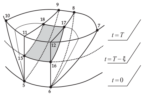
Figure 2: Domain $K^{T}_{\sigma}$

A dynamical system associated with the problem

$$v_{tt}-c^{2}\Delta v=0 {\text{in}}\,\,\,K^{T}_{\sigma}$$ (3.12)

$$v|_{t=T}=0,\,\,\,v_{t}|_{t=T}=y {\text{in}}\,\,\,\overline{\Omega^{T}_{\sigma}}$$ (3.13)

$$v=0 {\text{on}}\,\,\,\sigma^{T}\!\times\![0,T]$$ (3.14)

is called dual to system $\alpha^{T}_{\sigma}$; by $v=v^{y}(x,t)$ we denote its solution. Owing to the FDI, such a problem turns out to be well possed for any $y\in{\cal H}^{T}_{\sigma}$. Its peculiarity is that the Cauchy data are assigned to the final moment $t=T$, so that the problem is solved in reversed time.

The solutions to the original and dual problems obey the duality relation: for any $f\in{\cal F}^{T}_{\sigma}$ and $y\in{\cal H}^{T}_{\sigma}$, the equality

$$\left(u^{f}(\cdot,T),y\right)_{{\cal H}^{T}_{\sigma}}\,=\,\left(f,v^{y}_{\nu}\right)_{\mathcal{F}^{T}_{\sigma}}$$ (3.15)

is valid [5, 6, 7, 9].

$\bullet$  With the dual system one associates an observation operator $O^{T}:{\cal H}^{T}_{\sigma}\to{\cal F}^{T}_{\sigma}$,

$$O^{T}y\,:=\,v^{y}_{\nu}\big{|}_{\Sigma^{T}_{\sigma}}\,.$$

Writing (3.15) in the form $\left(W^{T}f,y\right)_{{\cal H}^{T}_{\sigma}}\,=\,\left(f,O^{T}y\right)_{\mathcal{F}^{T}_{\sigma}}$, we get an operator equality $O^{T}\,=\,(W^{T})^{*}$. Hence, the definition of $C^{T}$ implies

$$C^{T}\,=\,O^{T}W^{T}\,.$$ (3.16)

3.4 Projections of harmonic functions

$\bullet$  Assume that $y$ in (3.13) is harmonic: $y=a\in{\cal H}^{T}_{\sigma}$ obeys $\Delta a=0$ in $\Omega^{T}_{\sigma}$ and is continuously differentiable up to $\sigma^{T}\subset\partial\Omega^{T}_{\sigma}$. A simple integration by parts in (3.15) leads to

$$\left(a,u^{f}(\cdot,T)\right)_{\mathcal{H}^{T}_{\sigma}}=\left(O^{T}a,f\right)_{\mathcal{F}^{T}_{\sigma}}=$$

$$=\int_{\sigma^{T}\times[0,T]}(T-t)\left[a(\gamma)(R^{T}f)(\gamma,t)-a_{\nu}(\gamma)f(\gamma,t)\right]\,d\Gamma dt$$ (3.17)

(see [5, 6, 9, 10]).

Assume that $\{f^{\xi}_{k}\}_{k=1}^{\infty}\subset{\cal F}^{T,\xi}_{\sigma}$ is chosen in accordance with Convention 3 and produces the wave basis $\{u^{\xi}_{k}\}_{k=1}^{\infty}\subset{\cal H}^{\xi}_{\sigma}$. Then, representation (3.11) takes the form

$$P^{\xi}_{\sigma}a\,=\,\lim\limits_{N\to\infty}\sum\limits_{k=1}^{N}c^{\xi}_{k,N}u^{\xi}_{k}\,,$$ (3.18)

where $C^{\xi}_{N}=\{c^{\xi}_{k,N}\}_{k=1}^{N}$ satisfies the linear system

$${\cal G}^{\xi}_{N}C^{\xi}_{N}\,=\,B^{\xi}_{N}$$ (3.19)

with the Green matrix

$${\cal G}^{\xi}_{N}\,\overset{(\ref{Gramm G})}{=}\,\,\left\{2^{-1}(R^{2T}_{\sigma}JS^{T}f^{\xi}_{i},S^{T}f^{\xi}_{j})_{{\cal F}^{2T}_{\sigma}}\right\}_{i,j=1}^{N}\,=$$

$$=\left\{2^{-1}\int_{\sigma\times[0,2T]}(R^{2T}_{\sigma}JS^{T}f^{\xi}_{i})(\gamma,t)\,(S^{T}f^{\xi}_{j})(\gamma,t)\,d\Gamma dt\right\}_{i,j=1}^{N}$$ (3.20)

and the right-hand side

$$B^{\xi}_{N}=\{(a,u^{\xi}_{k})_{\cal H}\}_{k=1}^{N}\,,\quad(a,u^{\xi}_{k})_{\cal H}\overset{(\ref{(a,u^f)})}{=}$$

$$=\,\int_{\sigma^{T}\times[0,T]}(T-t)\left[a(\gamma)(R^{T}f^{\xi}_{k})(\gamma,t)-a_{\nu}(\gamma)f^{\xi}_{k}(\gamma,t)\right]\,d\Gamma dt\,.$$

With regard to (3.3),(3.4), and Convention 2, the latter can be written in the form

$$B^{\xi}_{N}=\left\{\int_{\sigma^{T}_{*}\times[0,T]}(T-t)\left[a(\gamma)(R^{2T}_{\sigma}S^{T}f^{\xi}_{k})(\gamma,t)-a_{\nu}(\gamma)f^{\xi}_{k}(\gamma,t)\right]\,d\Gamma dt\right\}_{k=1}^{N}$$ (3.21)

determined by $R^{2T}_{\sigma}$ and, thus, relevant for the further use.

$\bullet$   Fix a positive $\xi<T$. The operator

$$P^{\xi}_{\sigma\bot}:=P^{T}_{\sigma}-P^{\xi}_{\sigma}$$

is the projector in $\cal H$ onto the subspace ${\cal H}^{T}_{\sigma}\ominus{\cal H}^{\xi}_{\sigma}$; it cuts off functions on the subdomain $\Omega^{T}_{\sigma}\setminus\Omega^{\xi}_{\sigma}$.

Choose systems $\{f^{T}_{k}\}_{k=1}$ and $\{f^{\xi}_{k}\}_{k=1}$, which are linearly independent and complete in ${\cal F}^{T}_{\sigma}$ and ${\cal F}^{T,\xi}_{\sigma}$ respectively. Applying the (bounded) observation operator to (3.18), with regard to $O^{T}u^{f}=O^{T}W^{T}f\overset{(\ref{C^T=OW})}{=}C^{T}f$, we obtain

$$O^{T}P^{T}_{\sigma}a\,=\,\lim\limits_{N\to\infty}\sum\limits_{k=1}^{N}c^{T}_{k,N}C^{T}f^{T}_{k},\quad O^{T}P^{\xi}_{\sigma}a\,=\,\lim\limits_{N\to\infty}\sum\limits_{k=1}^{N}c^{\xi}_{k,N}C^{T}f^{\xi}_{k}\,.$$

Subtracting, we arrive at the representation

$$O^{T}P^{\xi}_{\sigma\bot}a\,=\,\lim\limits_{N\to\infty}\sum\limits_{k=1}^{N}\left[c^{T}_{k,N}C^{T}f^{T}_{k}-c^{\xi}_{k,N}C^{T}f^{\xi}_{k}\right]\,.$$ (3.22)

For the future application to the inverse problem, a crucial fact is that its right-hand side is determined by the response operator. Indeed, if $R^{2T}_{\sigma}$ is given, one can

1. choose the complete linearly independent systems $\{f^{T}_{k}\}^{\infty}_{k=1}\subset{\cal F}^{T}_{\sigma}$ and $\{f^{\xi}_{k}\}^{\infty}_{k=1}\subset{\cal F}^{T,\xi}_{\sigma}$; then, compose the Gramm matrices ${\cal G}^{T}_{N}$, ${\cal G}^{\xi}_{N}$ by (3.20) and columns $B^{T}_{N}$, $B^{\xi}_{N}$ by (3.21)

2. solving system (3.19) with respect to $C^{T}_{N}$, $C^{\xi}_{N}$, find the coefficients $c^{T}_{k,N},\,c^{\xi}_{k,N}$

3. determine $C^{T}$ by (3.6), compose the sum in (3.22) and, extending $N$, pass to the limit.

3.5 Amplitude formula

In what follows, we deal with the regular case $T<T_{\sigma}$.

$\bullet$   Fix a positive $\xi<T$; let $y$ be a smooth function in $\Omega$. Return to the dual system (3.12)–(3.14) and put

$$v_{t}\big{|}_{t=T}\,=\,P^{\xi}_{\sigma\bot}y\,=:\,y^{\xi}_{\bot}\,$$

in Cauchy data (3.13). Such a $y^{\xi}_{\bot}$ is of two specific features:

($i$)   it vanishes in $\Omega^{\xi}_{\sigma}$, so that ${\rm supp}\,y^{\xi}_{\bot}$ is separated from $\sigma$ by the $c$-distance $\xi$. Therefore, by the finiteness of the wave propagation speed, $v^{y^{\xi}_{\bot}}$ vanishes in the space-time domain $\{(x,t)\in K^{T}_{\sigma}\,|\,\,t>(T-\xi)+\tau(x,\sigma)\}$ and, in particular, one has

$$v^{y^{\xi}_{\bot}}_{\nu}(\cdot,t)\big{|}_{\sigma}\,=\,0\qquad{\rm for}\,\,T-\xi<t\leq T\,.$$ (3.23)

($ii$)  $y^{\xi}_{\bot}$ is discontinuous: generically, it has jumps at the equidistant surfaces $\Gamma^{T}_{\sigma}$ and $\Gamma^{\xi}_{\sigma}$. In particular, at the points $x(\gamma,\xi)\in B^{T}_{\sigma}\cap\Gamma^{\xi}_{\sigma}$, the value (amplitude) of the jump is

$$y^{\xi}_{\bot}(x(\gamma,\xi+0))\,=\,y(x(\gamma,\xi))\,.$$ (3.24)

$\bullet$   In hyperbolic equations theory, the well-known fact is that discontinuous Cauchy data initiate discontinuous solutions, the discontinuities propagating along characteristics. In our case of the wave equation (3.12), the jumps of $v_{t}\big{|}_{t=T}=y^{\xi}_{\bot}$ induce the jumps of $v^{y^{\xi}_{\bot}}_{t}$ in $K^{T}_{\sigma}$. In particular, there is a jump on the characteristic surface $\{(x,t)\in\overline{K^{T}_{\sigma}}\,|\,\,t=T-\xi+\tau(x,\sigma)\}$ including its smooth part $S^{T,\xi}_{\sigma}:=\{(x,t)\in\overline{K^{T}_{\sigma}}\,|\,\,x\in B^{T}_{\sigma}\}$ (on Fig 2, contoured by $\{15,16,17,18,15\}$). The jumps of $v^{y^{\xi}_{\bot}}_{t}$ on $S^{T,\xi}_{\sigma}$ and of $v^{y^{\xi}_{\bot}}_{\nu}$ on the cross-section $S^{T,\xi}_{\sigma}\cap\Sigma^{T}_{\sigma}=\{(\gamma,T-\xi)\,|\,\,\gamma\in\sigma\}$ (the line $\{15,16\}$) can be found by standard geometrical optics devices. For the latter jump, a simple analysis provides

$$v^{y^{\xi}_{\bot}}_{\nu}(\gamma,t)\big{|}^{t=T-\xi+0}_{t=T-\xi-0}\,=\,-\beta(\gamma,\xi)y(x(\gamma,\xi))\,,\qquad\gamma\in\sigma$$

(see, e.g., [2],[13],[9]). By (3.23), we have $v^{y^{\xi}_{\bot}}_{\nu}(\gamma,t)\big{|}^{t=T-\xi+0}=0$ that leads to

$$v^{y^{\xi}_{\bot}}_{\nu}(\gamma,T-\xi-0)\,=\,\beta(\gamma,\xi)y(x(\gamma,\xi))\,,\qquad\gamma\in\sigma\,.$$ (3.25)

Comparing (3.24) with (3.25), one can recall the well-known physical principle: jumps propagate along rays (here, a ray is $r^{\xi}_{\gamma}=\{x(\gamma,s)\,|\,\,0\leq s\leq\xi\}$) with the speed $c$, the ratio of the jump amplitudes at the input and output of the ray (here, at $x(\gamma,\xi)$ and $x(\gamma,0)$) depending on the ray spreading.

$\bullet$   Recalling the definitions of images and observation operator, one can write (3.25) in the form

$$(O^{T}P^{\xi}_{\sigma\bot}y)(\gamma,\xi)\,=\,\tilde{y}(\gamma,\xi)\,,\qquad(\gamma,\xi)\in\Sigma^{T}_{\sigma}\,.$$ (3.26)

It is the so-called amplitude formula (AF), which plays a central role in solving inverse problems by the BCM [5, 7, 9]. It represents the image of function in the form of collection of jumps, which pass through the medium, absorb information on the medium structure, and are detected by the external observer at the boundary.

$\bullet$   Now, let $y=a$ be a harmonic function. Combining (3.22) with (3.26), we arrive at the key relation

$$\tilde{a}(\gamma,\xi)\,=\,\lim\limits_{t\to T-\xi-0}\left\{\lim\limits_{N\to\infty}\left(\sum\limits_{k=1}^{N}\left[c^{T}_{k,N}\,C^{T}f^{T}_{k}-c^{\xi}_{k,N}\,C^{T}f^{\xi}_{k}\right]\right)(\gamma,t)\right\}\,,$$

$$(\gamma,\xi)\in\Sigma^{T}_{\sigma}\,.$$ (3.27)

As was noted at the end of section 3.4, to find its right-hand side, it suffices to know the response operator. In particular, since the coordinate functions are harmonic, applying (3.27) to $a=\pi^{i},\,\,i=0,\dots,n$ one can recover their images $\tilde{\pi}^{i}$ via $R^{2T}_{\sigma}$.

4 Determination of speed

4.1 Procedure

To solve the inverse problem, we just summarize our considerations in the form of the following procedure. Recall that the role of the procedure input data is played by operator $R^{2T}_{\sigma}$.

Step 1.   Fix a $\xi<T$. Applying the procedure $1.-3.$ described at the end of section 3.4, find the right-hand side of (3.27) for $a=\pi^{0},\pi^{1},\dots,\pi^{n}$ and, thus, get the images $\tilde{\pi}^{i}(\gamma,\xi)$ for $\gamma\in\sigma$.

Step 2.  Varying $\xi$, find $\tilde{\pi}^{i}$ on $\Sigma^{T}_{\sigma}$. Then, recover the map $\Sigma^{T}_{\sigma}\ni(\gamma,\xi)\mapsto x(\gamma,\xi)\in{\mathbb{R}}^{n}$ by the first representation in (2.3). The image of the map is $B^{T}_{\sigma}$, so that the ray tube is recovered in $\Omega$.

Step 3.   Differentiating with respect to $\xi$, find $c$ by the second representation in (2.3). The pairs $\{x(\gamma,\xi),c(x(\gamma,\xi))\,|\,\,(\gamma,\xi)\in\Sigma^{T}_{\sigma}\}$ constitute the graph of $c$ in $B^{T}_{\sigma}$.

Thus, the sound speed in the tube is determined. The following is some comments and remarks.

$\bullet$  For applications in geophysics, by the obvious reasons, it is desirable to minimize the part of the boundary, on which the external observer has to implement measurements. As is seen from (3.21), our procedure requires observations not only on $\sigma$ but on $\Gamma\backslash\sigma$, whereas the knowledge of the bound $c_{*}$ just enables the observer to restrict measurements on $\sigma^{T}_{*}$. In principle, one can avoid the observations on $\Gamma\backslash\sigma$ by the use of the artificial coordinates instead of the Cartesian $\pi^{i}$. Namely, one can choose the harmonic functions $a^{1},\dots,a^{n}$ obeying $a^{i}\big{|}_{\Gamma\backslash\sigma}=0$, which separate points of the tube $B^{T}_{\sigma}$ at least locally. By this choice, in (3.21) one gets $\int_{\sigma^{T}_{*}\!\times\![0,T]}=\int_{\sigma\!\times\![0,T]}$. Therefore, possessing the values of $R^{2T}_{\sigma}f$ on ${\sigma\!\times\![0,2T]}$ (but not on the whole $\Theta^{2T}_{\sigma}$!), one can recover the images $\tilde{a}^{i}$ via the amplitude formula and use them for identifying the points of $B^{T}_{\sigma}$ in $\Omega$. Thereafter, one recovers $c\big{|}_{B^{T}_{\sigma}}$. However, it is not clear, whether this plan can provide workable numerical algorithms.

$\bullet$   As was mentioned in 1.1, the procedure [5] (sections 7.6, 7.7) enables one to determine $c\big{|}_{\Omega^{T}_{\sigma}}$ from observations on ${\sigma\!\times\![0,2T]}$ only, and, thus, provides the strongest uniqueness result. However, its numerical implementation in the case of the time-domain inverse data seems to be rather problematic.

4.2 Numerical testing

Preparation of tests

$\bullet$   We take

$$\Omega:=\{(x^{1},x^{2})\in{\mathbb{R}}^{2}\,|\,\,x^{2}\leq 0\}\,,\quad\Gamma:=\{(x^{1},0)\in{\mathbb{R}}^{2}\,|\,\,-\infty<x^{1}<\infty\}\,,$$

$$\sigma:=\{x\in\Gamma\,|\,\,-L\leq x^{1}\leq L\}\,,$$

and consider a few concrete examples of the density $\rho=c^{-2}$ in $\Omega$.

$\bullet$  We choose an appropriate finite system of controls $f_{k}$ supported on $\sigma\times[0,T]$, the system being the same for all examples except Test $1(b)$ where results with another spatial basis are presented for comparison. It is well adapted to constructing the systems of delayed controls: for intermediate $\xi=\xi_{l}$, the shifts $f_{k}^{\xi_{l}}(\cdot,t)=f_{k}(\cdot,t-(T-\xi_{l}))$ are in use. This enables one to reduce considerably the computational resources.

$\bullet$   At each of the examples, we solve numerically the forward problems (1.1)–(1.3) with the final moments $t=T$ and $t=2T$ for the controls $f^{\xi_{l}}_{i}$ and ${JS^{T}f^{\xi_{l}}_{i}}$ respectively. These problems are solved by the use of a semi-discrete central-upwind third order accurate numerical scheme with WENO reconstruction suggested in [17]. As a result, we get the functions $u^{f^{\xi_{l}}_{i}}_{\nu}=R^{T}f^{\xi_{l}}_{i}=(R^{2T}_{\sigma}S^{T}f^{\xi_{l}}_{i})\big{|}_{0\leq t\leq T}$ and $u^{JS^{T}f^{\xi_{l}}_{i}}_{\nu}=R^{2T}_{\sigma}JS^{T}f^{\xi_{l}}_{i}$ entering in (3.21) and (3.20).

Controls

The BCM uses a system of boundary controls $f_{1},\,f_{2},\,\dots$, which belong to the Sobolev class:

$$\left\{f_{k}\in H^{1}(\Gamma\times[0,T])\mid f_{k}(\gamma,t)|_{t=0}=0\right\}$$

and constitute a basis in $L_{2}(\Gamma\times[0,T])$. We construct such a system from the products of elements of spatial and temporal bases, $f_{k}(\gamma,t)=\phi_{l}(\gamma)\,\psi_{m}(t)$, $k=l+mN_{\gamma}$, where $l={0:N_{\gamma}-1}$, $m={0:N_{t}-1}$, and the basis dimension is $N=N_{\gamma}N_{t}$.

In the case of the half-plane, we can keep under control only a part of the boundary and thus have to use localized basis functions. The simplest and good choice is a conventional trigonometric basis reduced to the interval $[-1,1]$ by an exponential cutoff multiplier $\eta(\gamma)=1/(1+\exp\left(\gamma/s\right))$ with a cutoff scale $s$, so that

$$\phi_{l}(\gamma)=\eta(\gamma-1)\,\eta(-\gamma-1)\,\cos\left[\pi\left(\frac{l}{2}+\lfloor\frac{l+1}{2}\rfloor(\gamma-1)\right)\right]\,,$$ (4.1)

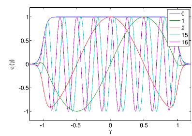
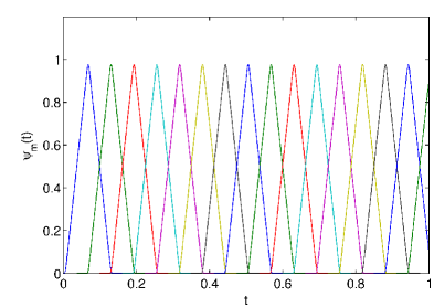
Figure 3: Basis of boundary controls: spatial functions $\phi_{l}(\gamma)$ with $l={0:16}$ and $s=1/32$ (left) and temporal functions $\psi_{m}(t)$ with $m={0:15}$ and $T=1$, $N_{t}=16$, $d=\Delta/64$ (right).

where $\lfloor\cdot\rfloor$ is the integer part. The spatial basis functions are shown in the left panel of Fig. 3.

The temporal basis is constructed from the shifts of a tent-like function,

$$\theta(t)=\frac{d}{\Delta}\,\left(1-\exp\left[-\frac{\Delta}{d}\right]\right)^{-1}\ln\left[\frac{\cosh\left[\frac{2\Delta-t}{2d}\right]\cosh\left[\frac{t}{2d}\right]}{\cosh^{2}\left[\frac{\Delta-t}{2d}\right]}\right],$$ (4.2)

so that $\psi_{m}(t)=\theta(t-m\Delta-\delta)$, where $\Delta=T/N_{t}$, $d$ is a smoothing parameter (when $d\rightarrow 0$ the function $\theta(t)$ gets a triangular shape), and $\delta$ is an offset to ensure a negligible value of $\theta(0)$. Such a shift-invariant basis (shown in the right panel of Fig. 3) considerably reduces computational resources needed for the BCM-reconstruction.

Regularization

$\bullet$   In the course of determination of $c$ by the procedure Step 1-3, we use the above-prepared data for computing the entries of $B^{\xi_{l}}_{N}$ and ${\cal G}^{\xi_{l}}_{N}$ in (3.21) and (3.20). Then the system (3.19) is solved for $a=\pi^{0},\pi^{1},\pi^{2}$, and the solutions $C^{\xi_{l}}_{N}$ are calculated by standard LAPACK routines.

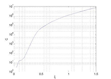
Figure 9: Test 2. The condition number of matrix (3.20) of scalar products as function of the probing time $\xi$.

Solving system (3.19), we have to apply a regularization procedure since the condition number of the Green matrix ${\cal G}^{\xi_{l}}_{N}$ rapidly grows as its size $N$ increases, see Figure 9. Because of unavoidable errors in matrix elements and right hand sides, the expansion coefficients $C^{\xi_{l}}_{N}$ also contain errors amplified by ill-conditioned matrix. We use Tikhonov’s regularization to reduce fake oscillations caused by errors in expansion coefficients. The value of regularization parameter is selected to satisfy a desired tolerance for residual of the linear system.

$\bullet$   One more operation, which produces unavoidable errors, is computation of the double limit in (3.27). The origin of the errors is the following.

In (3.18), the projection $P^{\xi}_{\sigma}a$ is a piece-wise smooth function in $\Omega$, which has a jump at the surface $\Gamma^{\xi}_{\sigma}$. Therefore, the convergence of the sums in the right hand side not uniform near $\Gamma^{\xi}_{\sigma}$, and the Gibbs oscillations do occur in the summation process. These oscillations are transferred to the amplitude formula (3.27) and considerably complicate the determination of jump at $t=T-\xi$, whereas this determination is a crucial point of the algorithm.

To damp this negative effect we apply the following procedure. The basis functions have finite resolution of the order of spatial-temporal scales of the highest harmonic. All scales below the minimum ones are unreachable, therefore we average the result of expansions (3.27) over that minimum scales by convolution with some kernel $K(\gamma,\xi)$,

$$\langle g\rangle(\gamma,t)=\int\limits_{-\infty}^{+\infty}\mathrm{d}t^{\prime}\int\limits_{-\infty}^{+\infty}\mathrm{d}\gamma^{\prime}K(\gamma-\gamma^{\prime},t-t^{\prime})\,g(\gamma^{\prime},t^{\prime}).$$ (4.3)

In our implementation the kernel $K(\gamma-\gamma^{\prime},t-t^{\prime})$ is a product of conventional Gaussian kernels both for spatial and temporal variables. Such a procedure efficiently removes the Gibbs oscillations and, in fact, accelerates convergence of the expansions. The values of standard deviations in the Gaussian kernels should match the minimum spatial and temporal scales of the boundary controls to smooth out the oscillations.

$\bullet$   At the final step, the speed $c$ is found by (2.3) with the help of numerical differentiation by the central finite difference formula.

Numerical results

Test 1.    Let

$$\rho(x^{1},x^{2})=1+a\,g_{1}(x^{1})\,g_{2}(x^{2}),\quad g_{k}(x^{k})=\exp{\left[-\frac{\left(x^{k}-\bar{x}^{k}\right)^{2}}{2\Delta_{k}^{2}}\right]},$$ (4.4)

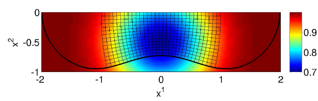
Figure 4: Test 1. Speed of sound $c(x)$ (color), exact semigeodesic coordinates (mesh), and wave front at $t=T$ (line).

where $a=1$, $\bar{x}^{1}=0$, $\bar{x}^{2}=-0.5$, $\Delta_{1}=0.5$, $\Delta_{2}=0.5$. The sound speed $c=\rho^{-\frac{1}{2}}$ is shown on Figure 4 together with exact semigeodesic coordinates and wave front at $t=T=1$. We test the recovering procedure for two rather different spatial bases (the temporal basis (4.2) consisting of 16 functions is the same in both cases).

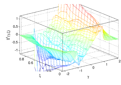
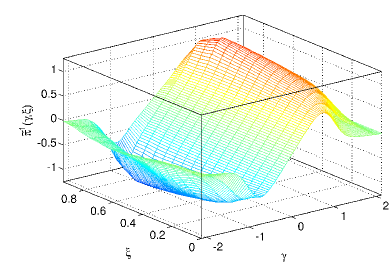
Figure 5: Test 1. Image $\tilde{\pi}^{1}(\gamma,\xi)$: expression (3.27) (left) and its smoothed version (4.3) (right).

a)  In this subcase, we use spatial basis composed from localized trigonometric functions (4.1). A typical image of harmonic function $x^{1}$ is shown in Figure 5, where we observe the Gibbs oscillations on the left plot and the smoothing effect of convolution (4.3) on the right one. The condition number of matrix (3.20) for $\xi=T$ is $1.5{\cdot}10^{5}$ and parameter of Tikhonov regularization for all linear systems is $1{\cdot}10^{-5}$. The standard deviations of Gaussian kernels in (4.3) for $(\gamma,t)$ are $\sigma_{\gamma}=0.1875$ and $\sigma_{t}=0$.

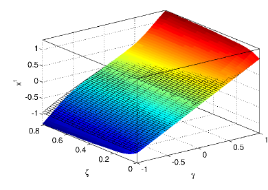
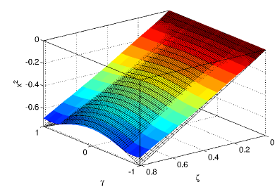
Figure 6: Test 1. Reconstructed mapping $x=x(\gamma,\xi)$, the exact values are shown by black mesh.

The mapping $x(\gamma,\xi)$ is shown in Figure 6. The reconstruction error grows towards the ends of the localization interval $\gamma\in(-1,1)$ and for large values of $\xi\approx T$.

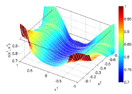
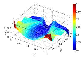
Figure 7: Test 1. Speed of sound $c(x)$ in the domain filled by waves initiated from $\sigma$: left - exact values, central - recovered values with trigonometric spatial basis, right - recovered values with tent-like spatial basis.

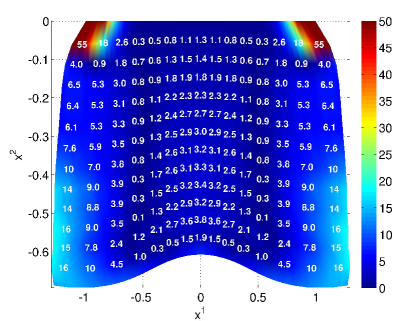
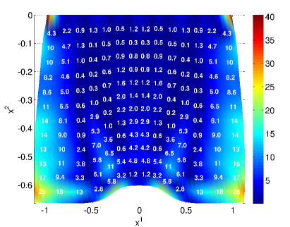
Figure 8: Test 1. Map of relative errors (in percents) of the recovered sound speed $c(x)$: left - with trigonometric spatial basis, right - with tent-like spatial basis.

The end result of the BCM is the sound speed recovered in the Cartesian coordinates. It is shown in central panel of Figure 7. Relative errors of reconstruction in percents are shown in left panel of Figure 8. As is seen, although the reconstruction error quickly grows towards the ends of the localization interval and for large values of $\xi\approx T$, in the most part of the domain covered by the direct rays from the boundary, the relative error does not exceed a few percents.

b)   Here we use a spatial basis composed from smooth tent-like functions as in (4.2). The condition number of matrix (3.20) for $\xi=T$ is $5.9{\cdot}10^{3}$ and parameter of Tikhonov regularization for all linear systems is $1{\cdot}10^{-6}$. The standard deviations of Gaussian kernels in (4.3) for $(\gamma,t)$ are $\sigma_{\gamma}=0.125$ and $\sigma_{t}=0.0625$. The recovered speed of sound is shown in right panel of Figure 7 while its relative errors are shown in right panel of Figure 8.

We may conclude that both of these bases provide similar quality of reconstruction of the order of several percents in most part of the domain. The advantages of the tent-like basis are smaller condition number of the system matrix and the same spatial scale of all basis functions. The effect of lower accuracy of reconstruction along the lateral boundaries in the case (b) is due to narrower support (smaller value of $L$) of the boundary controls compared to the case (a).

Test 2.    For the second test, we take

$$\rho(x^{1},x^{2})=1-0.5x^{2}+0.0625\left(x^{1}\right)^{2}-a\,g_{1}(x^{1})\,\frac{\partial g_{2}(x^{2})}{\partial x^{2}},$$

where $a=0.25$, $\bar{x}^{1}=0$, $\bar{x}^{2}=-0.5$, $\Delta_{1}=0.5$, $\Delta_{2}=0.25$. The corresponding sound speed has a background value $1$ and two variations of the order 30% of its boundary value.

We use $T=1.5$ and the basis with 16 spatial (trigonometric) and 32 temporal functions. The condition number of matrix (3.20) is shown in Figure 9; it grows as $\xi^{4}$. This is a consequence of the strong ill-posedness of the inverse problem under consideration, and such a growth constrains the maximal depth of reconstruction (determined by errors in right hand sides (3.21)), which is possible for the given part of the boundary. In computations, the parameter of Tikhonov regularization for all linear systems is fixed and equal to $1{\cdot}10^{-4}$. The standard deviations of Gaussian kernels in (4.3) for $(\gamma,t)$ are $\sigma_{\gamma}=0.1875$ and $\sigma_{t}=4.6875{\cdot}10^{-2}$. For $\xi\approx T$, the error in the expansion coefficients $a^{\xi}_{\alpha}$ grows up and we had to increase $\sigma_{\gamma}$ to the value $0.5$ for smoothing out the large scale fake oscillations from low spatial harmonics. Such an over-smoothing reduces the accuracy of the recovering for $\xi\approx T$.

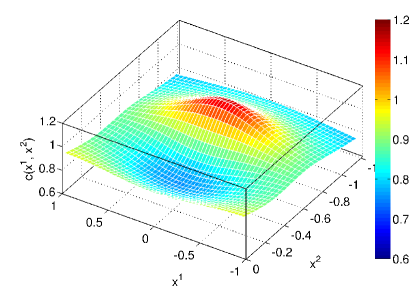
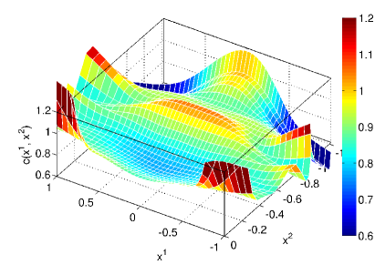
Figure 10: Test 2. Speed of sound $c(x)$ in the domain filled by waves initiated from $\sigma$: left - exact values, right - recovered values.

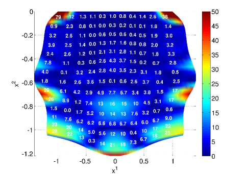
Figure 11: Test 2. Map of relative errors of the recovered sound speed in percents.

The recovered speed of sound in the Cartesian coordinates is shown in Figure 10, and relative errors of reconstruction in percents are shown in Figure 11. Thus, in the most part of the domain $\Omega_{\sigma}$ covered by the direct rays coming from $\sigma$, the relative error does not exceed a few percents.

Test 3.    Here we take

$$\rho(x^{1},x^{2})=1-0.5x^{2}+0.0625\left(x^{1}\right)^{2}+a\,g_{1}(x^{1})\,\left(1-x^{2}\right)\,\frac{\partial g_{2}(x^{2})}{\partial x^{2}},$$

where $a=0.25$, $\bar{x}^{1}=0$, $\bar{x}^{2}=-0.5$, $\Delta_{1}=0.5$, $\Delta_{2}=0.25$. In contrast to the case 2, the corresponding speed of sound has rather strong variations (the ratio of maximum to minimum value is about $2.5$).

Again, we take $T=1.5$ and use the basis with 16 spatial and 32 temporal functions. The condition number of matrix (3.20) for $\xi=T$ is $2{\cdot}10^{5}$ and in calculations the parameter of Tikhonov regularization for all linear systems is $1{\cdot}10^{-4}$. The standard deviations of Gaussian kernels in (4.3) for $(\gamma,t)$ are $\sigma_{\gamma}=0.1875$ and $\sigma_{t}=4.6875{\cdot}10^{-2}$. Again, for $\xi\approx T$ we had to increase $\sigma_{\gamma}$ to value $0.625$ to smooth out large scale fake oscillations from the low spatial harmonics.

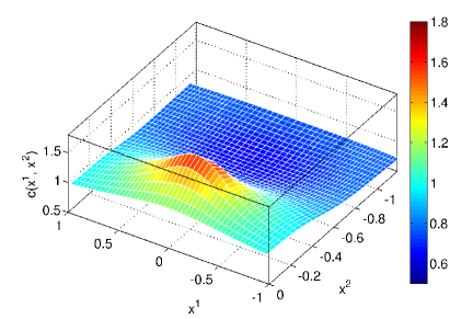
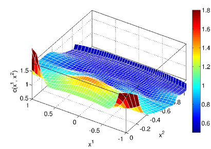
Figure 12: Test 3. Speed of sound $c(x)$ in the domain filled by waves initiated from $\sigma$: left - exact values, right - recovered values.

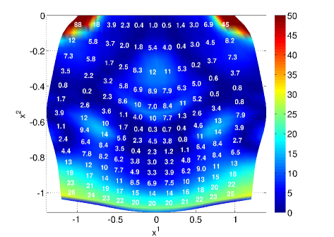
Figure 13: Test 3. Map of relative errors of the recovered sound speed in percents.

The recovered speed of sound in the Cartesian coordinates is shown in Figure 12, and relative errors of reconstruction in percents are shown in Figure 13.

Test 4.    To test the recovering algorithm for the case of sound speed quickly varying along the boundary we set

$$\rho(x^{1},x^{2}) =1-a\,g_{2}(z^{2})\,\frac{\partial g_{1}(z^{1})}{\partial x^{1}},$$

$$z^{1} =\cos(\phi)x^{1}+\sin(\phi)(x^{2}+0.25),$$

$$z^{2} =-\sin(\phi)x^{1}+\cos(\phi)(x^{2}+0.25),$$

where $a=0.25$, $\bar{x}^{1}=0$, $\bar{x}^{2}=0$, $\Delta_{1}=0.375$, $\Delta_{2}=0.25$, $\phi=\pi/12$.

We take $T=1$ and use the basis with 16 spatial and 32 temporal functions. The condition number of matrix (3.20) for $\xi=T$ is $1.28{\cdot}10^{5}$ and in calculations the parameter of Tikhonov regularization for all linear systems is $1{\cdot}10^{-4}$. The standard deviations of Gaussian kernels in (4.3) for $(\gamma,t)$ are $\sigma_{\gamma}=0.125$ and $\sigma_{t}=3.125{\cdot}10^{-2}$. Again, for $\xi\approx T$ we had to increase $\sigma_{\gamma}$ to the value $0.25$ in order to decrease large scale fake oscillations from the low spatial harmonics.

The recovered speed in the Cartesian coordinates is shown in Figure 14, and relative errors of reconstruction in percents are shown in Figure 15. We observe rather large oscillations in the speed values emerging at $x^{2}=-0.6$, and to demonstrate the origin of these oscillations we also show the results of a pseudo-reconstruction. The latter means the use of a conventional recovering procedure, in which all the matrix elements (products $(u^{f_{i}},u^{f_{j}})$) are computed via the solutions $u^{f_{i}}$ found by solving the forward problem with the given (known) speed profile. Such products are much more accurate than the ones found via the inverse data, and therefore the errors in the expansion coefficients in (3.27) are greatly reduced in the pseudo-reconstruction. This leads to much better quality of recovering far from the boundary and clearly shows the effect of ill-posedness of the reconstruction procedure.

Test 5.    The purpose of the last test is to check the ability of BCM to work with strong gradients in the recovered quantities. We prepare the density of medium as a slightly smoothed wedge with density $\rho=5$ included in the homogeneous background with the constant density $\rho=1$, see Figure 16.

We take $T=1$ and use the basis with 16 spatial and 32 temporal functions. The condition number of matrix (3.20) for $\xi=T$ is $2.07{\cdot}10^{4}$ and in calculations the parameter of Tikhonov regularization for all linear systems is $1.0{\cdot}10^{-4}$. The standard deviations of the Gaussian kernels in (4.3) for $(\gamma,t)$ are $\sigma_{\gamma}=0.125$ and $\sigma_{t}=3.125{\cdot}10^{-2}$. Again, for $\xi\approx T$ we had to increase $\sigma_{\gamma}$ to the value $0.325$ in order to decrease large scale fake oscillations from the low spatial harmonics.

The recovered density in the Cartesian coordinates is shown in Figure 16, and relative errors of reconstruction for $c(x)$ in percents are shown in Figure 17. The location of the wedge is recovered with good accuracy and without systematic shifts, the maximum of recovered density is $4.68$ that corresponds to the relative error about $7\%$. The smearing of discontinuities is quite reasonable taking into account the spatial scales of boundary controls and the smoothing ranges, whereas the errors at the discontinuities are big, as it has to be. We may suggest that if the resolution of boundary controls is not enough to resolve spatial scales of the medium inhomogeneities, then the method will recover a smoothed averaged profile, which can be further improved by another high resolution methods.

Comments

$\bullet$   Our results on the numerical speed determination from the time domain data given at a part of the boundary demonstrate that the BCM-algorithm is workable and provides good reconstruction in the domain covered by the normal acoustic rays.

$\bullet$   The key step of the algorithm is inversion of a big-size Gram matrix ($N\sim 10^{2}-10^{3}$), which consists of the inner products of waves initiated by rich enough system of boundary controls. As is typical in multidimensional (strongly ill-posed) inverse problems, the condition number of this matrix rapidly grows as one extends the number of controls and/or the observation time. Therefore, to increase the depth of reconstruction one has to use controls acting from a larger part of the boundary or decrease errors in the input inverse data.

$\bullet$   The number and shape of boundary controls determine the spatial resolution of the reconstruction procedure. The BCM is able to work with low number of spatial controls: in such a case it provides an ‘averaged’ profile. As we hope, such a profile can be used as a starting approximation for high resolution iterative reconstruction methods .

In the future work, we plan to evaluate the influence of external noises in the inverse data on the quality of the BCM reconstruction, and apply the method to another domains and more realistic sound speed profiles.

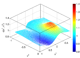
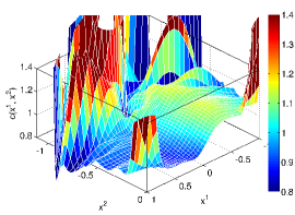
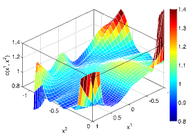
Figure 14: Test 4. Speed of sound $c(x)$ in the domain filled by waves initiated from $\sigma$: left - exact values, central - recovered values, right - pseudo-recovered values.

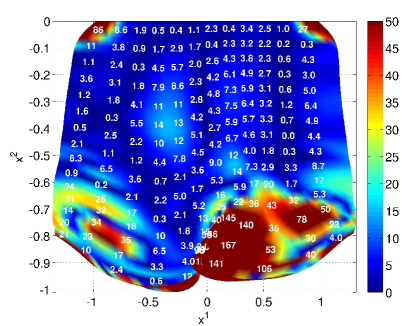
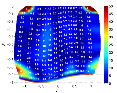
Figure 15: Test 4. Map of relative errors (in percents) of the recovered sound speed $c(x)$: left - usual reconstruction, right - pseudo-reconstruction.

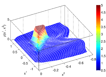
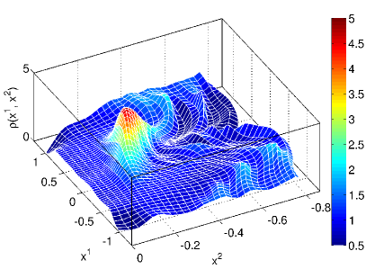
Figure 16: Test 5. Density of medium $\rho(x)$ in the domain filled by waves initiated from $\sigma$: left - exact values, right - recovered values.

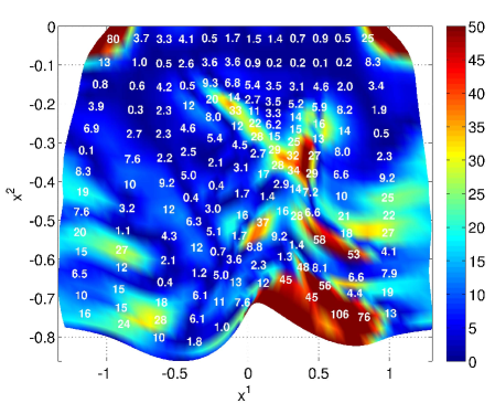
Figure 17: Test 5. Map of relative errors of the recovered sound speed in percents.

References

- [1] S.A.Avdonin, M.I.Belishev, S.A.Ivanov. Controllability in filled domains for the wave equation with singular controls. Zapiski Nauchnykh Seminarov POMI, 210 (1994), 3–14 (in Russian); English translation: JMS, 83(1997), no 2.
- [2] V.M.Babich and V.S.Buldyrev, Short-Wavelength Diffraction Theory. Asymptotic Methods. Springer-Verlag, Berlin, 1991.
- [3] , L.Beilina and M.V.Klibanov. Approximate Global Convergence and Adaptivity for Coefficient Inverse Problems. Springer, 2012.
- [4] M.I.Belishev. On an approach to multidimensional inverse problems for the wave equation. Soviet Mathematics. Doklady, 36 (1988), no 3, 481–484.
- [5] M.I.Belishev. Boundary control in reconstruction of manifolds and metrics (the BC-method). Inverse Problems, 13 (1997), no 5, R1–R45.
- [6] M.I.Belishev. How to see waves under the Earth surface (the BC-method for geophysicists). Ill-Posed and Inverse Problems, S.I.Kabanikhin and V.G.Romanov (Eds). VSP, Utrecht, Boston, 67–84, 2002.
- [7] M.I.Belishev. Recent progress in the BC-method. Inverse Problems, 23 (2007), no 5, R1–R67.
- [8] M.I.Belishev. Dynamical Inverse Problem for the Equation (the BC-method). CUBO A Mathematical Journal, 10 (2008), No 2, 17–33.
- [9] M.I.Belishev, A.S.Blagoveschenskii. Dynamical Inverse Problems of Wave Theory. SPb State University, St-Petersburg, 1999 (in Russian).
- [10] M.I.Belishev, V.Yu.Gotlib. Dynamical variant of the BC-method: theory and numerical testing. Journal of Inverse and Ill-Posed Problems, 7, no 3: 221–240, 1999.
- [11] M.I.Belishev, V.Yu.Gotlib, S.A.Ivanov. The BC-method in multidimensional spectral inverse problem: theory and numerical illustrations. Control, Optimization and Calculus of Variations, 2: 307–327, October, 1997.
- [12] M.I.Belishev, V.A.Ryzhov, V.B.Filippov. Spectral variant of the BC-method: theory and numerical experiment. Doklady Akad. Nauk SSSR, 332 (1994), No 4, 414–417 (in Russian). English translation: ?????.
- [13] M.Ikawa. Hyperbolic PDEs and Wave Phenomena. Translations of Mathematical Monographs, v. 189 AMS; Providence. Rhode Island, 1997.
- [14] V.Isakov. Inverse problems for partial differential equations. Appl. Math. Studies, Springer, v. 127, 1998.
- [15] S.I.Kabanikhin, M.A.Shishlenin, A.D.Satybaev. Direct Methods of Solving Inverse Hyperbolic Problems. Utrecht, The Netherlands, VSP, 2004.
- [16] S.I.Kabanikhin and M.A.Shishlenin. Numerical algorithm for two-dimensional inverse acoustic problem based on Gel’fand-Levitan-Krein equation. Journal of Inverse and Ill-Posed Problems, 18, no 9: 221–240, 2011.
- [17] A.Kurganov, S.Noelle, and G.Petrova. Semidiscrete central-upwind schemes for hyperbolic conservation laws and Hamilton–Jacobi equations. SIAM Journal on Scientific Computing, 23 (2001), no 3, 707–740.
- [18] L.Oksanen. Solving an inverse obstacle problem for the wave equation by using the boundary control method. Inverse Problems, 29 (2013), no 3, 035004; doi:10.1088/0266-5611/29/3/035004 http://iopscience.iop.org/0266-5611/29/3/035004/article?fromSearchPage=true.
- [19] L.N.Pestov. Inverse problem of determining absorption coefficient in the wave equation by BC method. Journal of Inverse and Ill-Posed Problems, 20, no 1: 103–110, 2012. ISSN (Online) 1569-3945, ISSN (Print) 0928-0219, DOI: 10.1515/jip-2011-0015, March 2012
- [20] L.N.Pestov. On determining an absorption coefficient and a speed of sound in the wave equation by the BC-method. Journal of Inverse and Ill-Posed Problems, 21, no 2: 245–250, 2013. ISSN (Online) 1569-3945, ISSN (Print) 0928-0219, DOI: 10.1515/jip-2013-0012, November 2013.
- [21] Pestov L., Kazarina O. Bolgova V. Numerical recovering a density by the boundary control method. Inverse Problems and Imaging, 2011. Vol. 4, no. 4, 703–712.
- [22] V.G.Romanov. A local version of a numerical method for solving an inverse problem. Siberian Math. J., 37 (1996), no 4, 797–810.