Chiral spin-orbital liquids with nodal lines

Abstract

Strongly correlated materials with strong spin-orbit coupling hold promise for realizing topological phases with fractionalized excitations. Here we propose a chiral spin-orbital liquid as a stable phase of a realistic model for heavy-element double perovskites. This spin liquid state has Majorana fermion excitations with a gapless spectrum characterized by nodal lines along the edges of the Brillouin zone. We show that the nodal lines are topological defects of a non-Abelian Berry connection and that the system exhibits dispersing surface states. We discuss some experimental signatures of this state and compare them with properties of the spin liquid candidate Ba₂YMoO₆.

Quantum spin liquids (QSLs) are Mott insulators in which quantum fluctuations prevent long-range magnetic order down to zero temperature Balents (2010). They have received both experimental and theoretical attention due to predictions of unusual phenomena such as spin-gapped phases with topological order or gapless phases without spontaneous breaking of continuous symmetries Wen (2004). In recent years the evidence for QSLs in nature has started to look more auspicious thanks to the discovery of new compounds that realize the Heisenberg model on frustrated lattices Han et al. (2012). While frustration is a desirable ingredient, seminal work by Kitaev Kitaev (2006) has demonstrated that bond-dependent exchange interactions may provide another route towards QSL ground states. The key idea is that a spin-$1/2$ model on the (bipartite) honeycomb lattice with judiciously chosen anisotropic interactions can be rewritten in terms of free Majorana fermions hopping in the background of a static Z₂ gauge field. The result is a QSL with exotic fractional excitations. The same idea has been applied to construct other exactly solvable models, including cases of higher spins Yao, Zhang, and Kivelson (2009); Mandal and Surendran (2009); Wu, Arovas, and Hung (2009); Hermanns and Trebst (2014); O’Brien, Hermanns, and Trebst (2016).

From a broader perspective, Kitaev’s model is an instance of a quantum compass model Dorier, Becca, and Mila (2005); Lacroix, Mendels, and Mila (2011); Nussinov and van den Brink (2015). Although Kitaev-type exactly solvable models are artificial, the kind of anisotropic interactions they presuppose arises naturally in Mott insulators with orbital degeneracy and strong spin-orbit coupling Jackeli and Khaliullin (2009); Chaloupka, Jackeli, and Khaliullin (2010). There is recent evidence that bond-dependent interactions are dominant in Na₂IrO₃ Hwan Chun et al. (2015). While this compound is in a zigzag-ordered phase at low temperatures, the prospect of finding QSLs in compass models suggests inspecting other families of heavy-element transition metal oxides Pesin and Balents (2010); Wan et al. (2011); Witczak-Krempa et al. (2014).

All the conditions leading to quantum compass models can be found in Mott-insulating rock-salt-ordered double perovskites Chen, Pereira, and Balents (2010). Given the chemical formula A₂BB^′O₆, particularly interesting properties are found in compounds where the B^′ magnetic ions have a 4d¹ or 5d¹ configuration. These ions are arranged in a face-centered-cubic (fcc) lattice, which, unlike the honeycomb lattice, is geometrically frustrated. The magnetic properties within this family are diverse Wiebe et al. (2002); Stitzer, Smith, and zur Loye (2002); Yamamura, Wakeshima, and Hinatsu (2006); Erickson et al. (2007), but the material that stands out is Ba₂YMoO₆ de Vries, Mclaughlin, and Bos (2010); Aharen et al. (2010); Carlo et al. (2011); de Vries et al. (2013). Despite a Curie-Weiss temperature $\Theta_{\text{cw}}\approx-160$ K de Vries, Mclaughlin, and Bos (2010), several experiments point to the absence of long-range order down to $T\sim 2$ K. Moreover, there is no sign of structural transitions, implying that the lattice remains cubic at low temperatures. Thus, the degeneracy of the $t_{2g}$ orbitals is only partially lifted by the spin-orbit coupling, leading to a low-lying $j=3/2$ quadruplet de Vries, Mclaughlin, and Bos (2010). The effective model contains bond-dependent interactions between nearest-neighbor $j=3/2$ spins and is closely related to $\Gamma$-matrix generalizations of Kitaev’s model Yao, Zhang, and Kivelson (2009); Wu, Arovas, and Hung (2009). Remarkably, the analysis in Chen, Pereira, and Balents (2010) revealed that, when antiferromagnetic exchange is dominant, ordered phases become unstable against quantum fluctuations, making this an interesting point to look for QSLs.

In this Letter we investigate a QSL in a realistic model for double perovskites with strong spin-orbit coupling. Using a representation of $j=3/2$ operators in terms of six Majorana fermions, we start by showing that a hidden SU(2) symmetry of the Hamiltonain becomes an explicit SO(3) symmetry for three of these fermions, whereas the other three exhibit a compass-model-type Z₃ symmetry. As the model is not exactly solvable, we proceed with a mean-field approach and propose a spin liquid ansatz that preserves the SO(3) and Z₃ symmetries. The ansatz breaks inversion and time reversal symmetry, thus describing a chiral spin liquid. Most interestingly, we find that the excitation spectrum is gapless along nodal lines which are vortices of a Berry connection in momentum space. This feature makes this chiral spin liquid a strongly correlated analogue of line-node semimetals and superconductors discussed in the context of topological phases of weakly interacting electrons Burkov, Hook, and Balents (2011); Chiu and Schnyder (2014); Yang, Pan, and Zhang (2014); Bian et al. (2016) and photonic crystals Lu et al. (2013). Going beyond the mean-field level, we use variational Monte Carlo (VMC) techniques Gros (1989); Ceperley, Chester, and Kalos (1977); Edegger et al. (2005) to show that our spin liquid state yields a remarkably low energy and should be regarded as a competitive candidate for the ground state of the spin-orbital model. Finally, we argue that the vanishing density of states at low energies predicted by our theory can account for some unusual properties observed in Ba₂YMoO₆.

The spin-orbital model for cubic double perovskites with d¹ electronic configuration is given by Chen, Pereira, and Balents (2010)

$$H=J\underset{\alpha,\langle ij\rangle\in\alpha}{\sum}\left(\textbf{S}_{i,\alpha}\cdot\textbf{S}_{j,\alpha}-\frac{1}{4}n_{i,\alpha}n_{j,\alpha}\right)-\lambda\sum_{i}\textbf{l}_{i}\cdot\textbf{S}_{i}.$$ (1)

Here $J>0$ is the antiferromagnetic exchange between nearest-neighbor spins and $\lambda>0$ is the atomic spin-orbit coupling. The index $\alpha$ labels both planes (XY, YZ or XZ) and $t_{2g}$ orbitals ($d_{xy}$, $d_{yz}$ or $d_{xz}$) Tokura and Nagaosa (2000). The operators $n_{i,\alpha}$ and $\textbf{S}_{i,\alpha}$ describe the number and the spin of electrons occupying the $\alpha$ orbital on site $i$, with the constraint $\sum_{\alpha}n_{i,\alpha}=1$, and $\mathbf{l}_{i}$ is the effective $l=1$ orbital angular momentum of the $t_{2g}$ states Ballhausen (1962). The total spin on site $i$ is $\mathbf{S}_{i}=\sum_{\alpha}\mathbf{S}_{i,\alpha}$.

In the regime $\lambda\gg J$, spin and orbital operators can be projected into the low-energy subspace of total angular momentum $j=3/2$ Chen, Pereira, and Balents (2010). The projected Hamiltonian $\tilde{H}=\mathcal{P}_{3/2}H\mathcal{P}_{3/2}$, where $\mathcal{P}_{3/2}$ is the projector, contains multipolar interactions in terms of $\mathbf{J}_{i}=\mathbf{l}_{i}+\mathbf{S}_{i}$. Our first step is to introduce operators $\mathbf{s}$ and $\bm{\tau}$ at each site as

$$\textbf{s}=\frac{1}{2}(-\Gamma^{23},\Gamma^{13},\Gamma^{12}),\quad\bm{\tau}=\frac{1}{2}(\Gamma^{4},-\Gamma^{45},\Gamma^{5}).$$ (2)

The notation refers to five Dirac $\Gamma$ matrices given explicitly by

$$\Gamma^{1} = \sigma^{z}\otimes\sigma^{y},\;\Gamma^{2}=\sigma^{z}\otimes\sigma^{x},\;\Gamma^{3}=\sigma^{y}\otimes\mathbbm{1},$$

$$\Gamma^{4} = \sigma^{x}\otimes\mathbbm{1},\;\Gamma^{5}=-\Gamma^{1}\Gamma^{2}\Gamma^{3}\Gamma^{4},$$ (3)

where $\sigma^{a}$, $a\in\{x,y,z\}$, are Pauli matrices, and 10 matrices $\Gamma^{\mu\nu}\equiv\left[\Gamma^{\mu},\Gamma^{\nu}\right]/(2i)$ Murakami, Nagaosa, and Zhang (2004); Yao, Zhang, and Kivelson (2009). The components of $\mathbf{s}$ and $\bm{\tau}$ satisfy the SU(2) algebra $[s^{a},s^{b}]=i\epsilon^{abc}s^{c}$, $[\tau^{a},\tau^{b}]=i\epsilon^{abc}\tau^{c}$, and $[s^{a},\tau^{b}]=0$. The relation between the basis of $J^{z}$ and the basis $|s^{z},\tau^{z}\rangle$, with $s^{z},\tau^{z}\in\{+,-\}$, is $\left|J^{z}=\pm\frac{3}{2}\right\rangle=|\mp,+\rangle,\left|J^{z}=\pm\frac{1}{2}\right\rangle=|\pm,-\rangle$.

In the new representation the projected Hamiltonian assumes a relatively simple form:

$$\tilde{H}=\frac{J}{9}\underset{\langle i,j\rangle\in\alpha}{\sum}\left(\textbf{s}_{i}\cdot\textbf{s}_{j}-\frac{1}{4}\right)(1-2\tau_{i}^{\alpha})(1-2\tau_{j}^{\alpha}),$$ (4)

where $\tau^{\alpha}$ are given by $\tau^{xy}=\tau^{z}$, $\tau^{yz(xz)}={\frac{1}{2}(-\tau^{z}\pm\sqrt{3}\tau^{x})}$. A few comments are in order. First, Eq. (4) has the familiar form of a Kugel-Khomskii model Kugel and Khomski (1982); Feiner, Oleś, and Zaanen (1997). However, here the Kugel-Khomskii coupling involves pseudospins $\mathbf{s}$ and pseudo-orbitals $\bm{\tau}$ defined in the $j=3/2$ subspace, where the original spins and orbitals are highly entangled. Second, the Hamiltonian commutes with $\mathbf{s}_{\text{tot}}=\sum_{i}\mathbf{s}_{i}$. This is a manifestation of the hidden global SU(2) symmetry discussed in Chen, Pereira, and Balents (2010). This continuous symmetry is unexpected, given that spin-orbit coupling breaks the conservation of $\mathbf{J}_{\text{tot}}=\sum_{i}\mathbf{J}_{i}$, but appears in related models for $t_{2g}$ orbitals Harris et al. (2003) and at special points of the Kitaev-Heisenberg model Chaloupka and Khaliullin (2015). Finally, the pseudo-orbital coupling has the form of a 120^∘ compass model Nussinov and van den Brink (2015). There is a Z₃ symmetry generated by $U_{3}=e^{-i\frac{2\pi}{3}\tau_{\text{tot}}^{y}}$ followed by a C₃ rotation of the $\alpha$ planes.

In analogy with the spin liquid in Kitaev’s model Kitaev (2006), we now introduce a Majorana parton representation for the generators of SU(4) (i.e. the basis of $j=3/2$ operators). We write $\mathbf{s}$ and $\bm{\tau}$ operators as Tsvelik (2007); Coleman, Miranda, and Tsvelik (1994); Wang and Vishwanath (2009); Biswas et al. (2011); Herfurth, Streib, and Kopietz (2013); Hermanns, O’Brien, and Trebst (2015)

$$s^{a}_{j}=-\frac{i}{4}\epsilon^{abc}\eta^{b}_{j}\eta^{c}_{j},\qquad\tau^{a}_{j}=-\frac{i}{4}\epsilon^{abc}\theta_{j}^{b}\theta^{c}_{j}.$$ (5)

The components of $\bm{\eta}_{j}$ and $\bm{\theta}_{j}$ are Majorana fermions that obey $\{\gamma_{j}^{a},\gamma_{l}^{b}\}=2\delta_{jl}\delta^{ab}$, where $\gamma\in\{\eta,\theta\}$. As the signs of the fermions can be changed ($\bm{\eta}\rightarrow-\bm{\eta}$, $\bm{\theta}\rightarrow-\bm{\theta}$) without affecting the physical operators, this representation bears a Z₂ redundancy. To eliminate the extra states, one can impose the local constraint Wang and Vishwanath (2009)

$$D_{j}\equiv i\eta^{1}_{j}\eta^{2}_{j}\eta^{3}_{j}\theta^{1}_{j}\theta^{2}_{j}\theta^{3}_{j},\qquad D_{j}=1\;\forall j.$$ (6)

With this constraint we have $s_{j}^{a}\tau_{j}^{b}=-\frac{i}{4}\eta^{a}_{j}\theta^{b}_{j}$ , and Hamiltonian (4) becomes quartic in Majorana fermions:

$$\tilde{H} = -\frac{NJ}{6}+\frac{J}{36}\sum_{\langle i,j\rangle\in\alpha}\left[\left(\sum_{a<b}\eta^{a}_{i}\eta^{a}_{j}\eta^{b}_{i}\eta^{b}_{j}\right)\right.$$ (7)

$$+(\eta^{1}_{i}\eta^{2}_{i}\eta^{3}_{j}+\eta^{2}_{i}\eta^{3}_{i}\eta^{1}_{j}+\eta^{3}_{i}\eta^{1}_{i}\eta^{2}_{j})\bar{\theta}^{\alpha}_{j}+(i\leftrightarrow j)$$

$$\left.+\bar{\theta}^{\alpha}_{i}\bar{\theta}^{\alpha}_{j}\bm{\eta}_{i}\cdot\bm{\eta}_{j}-\theta^{\alpha}_{i}\theta^{\alpha}_{j}\theta^{2}_{i}\theta^{2}_{j}\right],$$

where $N$ is the number of sites and $\theta^{\alpha}$ and $\bar{\theta}^{\alpha}$ are defined by $\theta^{xy}=\theta^{1}$, $\theta^{yz(xz)}=\frac{1}{2}(-\theta^{1}\mp\sqrt{3}\theta^{3})$, and $\bar{\theta}^{xy}=\theta^{3}$, $\bar{\theta}^{yz(xz)}=\frac{1}{2}(-\theta^{3}\pm\sqrt{3}\theta^{1})$.

Hamiltonian (7) is invariant under global SO(3) rotations of the $\bm{\eta}$ vector. The couplings involving the components of $\bm{\theta}$ have only a discrete symmetry, namely the octahedral point group symmetry O${}_{\text{h}}$ of the lattice. The latter contains the Z₃ that rotates $\theta^{\alpha}$ and $\bar{\theta}^{\alpha}$ by 120^∘ in the $(\theta^{1},\theta^{3})$ plane. In addition, $\tilde{H}$ is invariant under time reversal $T=Ke^{-i\pi J_{\text{tot}}^{y}}$, where $K$ denotes complex conjugation. In terms of Majorana fermions, $T=K\prod_{j}\theta_{j}^{1}\theta_{j}^{3}$.

Next, we perform a mean-field decoupling of Hamiltonian (7). This is equivalent to neglecting fluctuations of the Z₂ gauge field and yields qualitatively correct results as long as the system is in a QSL phase with deconfined Majorana fermions Tsvelik (2007). Our choice of mean field ansatz is guided by the condition of preserving the SO(3) and Z₃ symmetries. This restricts the set of nonzero parameters $\langle\gamma^{a}_{i}\gamma^{b}_{j}\rangle$. We obtain

$$\tilde{H}_{\text{MF}} = -\frac{NJ}{6}+\frac{J}{36}\underset{\langle j,l\rangle\in\alpha}{\sum}\left[i(2u_{jl}+\bar{w}^{\alpha}_{jl})\bm{\eta}_{j}\cdot\bm{\eta}_{l}\right.$$ (8)

$$+3iu_{jl}\bar{\theta}^{\alpha}_{j}\bar{\theta}^{\alpha}_{l}-iw^{\alpha}_{jl}\theta^{2}_{j}\theta^{2}_{l}-iv_{jl}\theta^{\alpha}_{j}\theta^{\alpha}_{l}$$

$$\left.+3u_{jl}^{2}+3\bar{w}^{\alpha}_{jl}u_{jl}-w^{\alpha}_{jl}v_{jl}\right],$$

where $iu_{jl}=\langle\eta^{a}_{j}\eta^{a}_{l}\rangle$, $iv_{jl}=\langle\theta^{2}_{j}\theta^{2}_{l}\rangle$, $iw^{\alpha}_{jl}=\langle\theta^{\alpha}_{j}\theta^{\alpha}_{l}\rangle$, and $i\bar{w}^{\alpha}_{jl}=\langle\bar{\theta}^{\alpha}_{j}\bar{\theta}^{\alpha}_{l}\rangle$ play the role of imaginary hopping amplitudes. Note that the symmetry implies decoupling of $\eta^{a}$ and $\theta^{2}$ fermions at the level of bilinear terms; yet, $\theta^{1}$ and $\theta^{3}$ remain coupled.

Seeking a translationally invariant ansatz, we set the order parameters to have uniform magnitude: $u_{ij}=u\sigma^{u}_{ij}$, $v_{ij}=v\sigma_{ij}^{v}$, $w^{xy}_{ij\in\text{XY}}=w\sigma^{w}_{ij}$, $\bar{w}^{xy}_{ij\in\text{XY}}=\bar{w}\sigma^{\bar{w}}_{ij}$, with $u,v,w,\bar{w}$ to be determined by self-consistent equations, whereas the $\sigma$’s are chosen to be $\pm 1$ on each bond. Since e.g. $u_{ij}=-u_{ji}$, the choice of $\sigma^{u}_{ij}$ is equivalent to a choice of bond orientation and determines the gauge-invariant flux through elementary plaquettes. Noticing that the fcc lattice can be viewed as a network of edge-sharing tetrahedra, we obtain a symmetric ansatz by requiring that the Z₂ fluxes, e.g. $\chi^{u}_{jkl}\equiv i\sigma^{u}_{jk}\sigma^{u}_{kl}\sigma^{u}_{lj}$, be the same on all faces of a given tetrahedron, with sites $jkl$ on every triangle oriented counterclockwise with respect to an outward normal vector. This leads to the four-sublattice ansatz illustrated in Fig. 1.

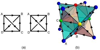
Figure 1: (color online). (a) Two gauge-inequivalent hopping configurations with the same flux of the Z₂ gauge field on all faces of a tetrahedron. (b) Four-sublattice ansatz on the fcc lattice. The sign of the outward flux alternates between edge-sharing tetrahedra (represented by different color fillings).

Let us discuss the symmetry of our ansatz. First, we note that the Z₂ gauge flux through triangles is odd under time reversal and is related to the spin chirality order parameter Baskaran (1989); Wen, Wilczek, and Zee (1989). The state also breaks inversion $P$; this can be seen from Fig. 1(b), since a mirror-plane reflection exchanges tetrahedra with opposite chiralities. Thus, our ansatz describes a chiral spin liquid with spontaneous breaking of $P$ and $T$. However, $PT$ is still a symmetry. Similarly, a projective symmetry group analysis Wen (2004) shows that broken rotational symmetries can be combined with the broken time reversal to restore an O${}_{\text{h}}$ point group symmetry, ensuring the orbital degeneracy assumed at the outset (see Supplemental Material Sup ).

Having fixed the ansatz, we can calculate the resulting spectrum of the Majorana fermions. For simplicity, first we focus on the mean-field Hamiltonian for $\gamma\in\{\eta^{a},\theta^{2}\}$, i.e., the flavors which are decoupled in Eq. (8). In this case the Hamiltonian can be written in the form

$$\tilde{H}_{\text{MF}}=\sum_{\mathbf{k}\in\frac{1}{2}\text{BZ}}\gamma^{\dagger}_{\mathbf{k}}\mathcal{H}(\mathbf{k})\gamma^{\phantom{\dagger}}_{\mathbf{k}}=|t|\sum_{\mathbf{k}\in\frac{1}{2}\text{BZ}}\gamma^{\dagger}_{\mathbf{k}}(\mathbf{h}_{\mathbf{k}}\cdot\bm{\Sigma})\gamma^{\phantom{\dagger}}_{\mathbf{k}},$$ (9)

where $t=t(u,v,w,\bar{w})$ is the corresponding hopping amplitude in Eq. (8), $\gamma_{\mathbf{k}}^{\dagger}=(\gamma_{\mathbf{k}\text{A}}^{\dagger},\gamma_{\mathbf{k}\text{B}}^{\dagger},\gamma_{\mathbf{k}\text{C}}^{\dagger},\gamma_{\mathbf{k}\text{D}}^{\dagger})$ is a spinor with components labeled by sublattice index, $\mathbf{h}_{\mathbf{k}}=4\left(\cos\frac{k_{x}}{2}\cos\frac{k_{y}}{2},\cos\frac{k_{y}}{2}\cos\frac{k_{z}}{2},\cos\frac{k_{z}}{2}\cos\frac{k_{x}}{2}\right)$, $\bm{\Sigma}=(-\Gamma^{1},-\Gamma^{3},\Gamma^{13})$, and the sum is restricted to half Brillouin zone since $\gamma^{\phantom{\dagger}}_{-\mathbf{k}}=\gamma^{\dagger}_{\mathbf{k}}$ Coleman, Miranda, and Tsvelik (1994). As the components of $\bm{\Sigma}$ obey $[\Sigma^{a},\Sigma^{b}]=i\epsilon^{abc}\Sigma^{c}$, the spectrum is given simply by

$$\varepsilon_{\pm}(\mathbf{k})=\pm|t||\mathbf{h}_{\mathbf{k}}|.$$ (10)

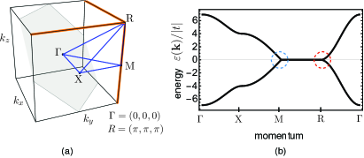
Figure 2: (color online). (a) Brillouin zone of the cubic sub-lattice. (b) Bulk dispersion. The nodal lines along MR directions cross at the quadratic band touching point R.

The dispersion relation is illustrated in Fig. 2. There are two doubly degenerate bands Sup . Since $\{P,\tilde{H}_{\text{MF}}\}=0$, the Hamiltonian has a chiral symmetry Wen and Zee (1989); Koshino, Morimoto, and Sato (2014) and the spectrum is symmetric between positive- and negative-energy states. The defining feature of the band structure is the band touching along the edges of the Brillouin zone. These are nodal lines parametrized, e.g., by $\mathbf{k}=(\pi,\pi,k_{z})$. Expanding $\mathbf{k}=(\pi+p_{x},\pi+p_{y},k_{z})$, with $p_{x},p_{y}\ll 1$, we obtain the effective Hamiltonian on a plane perpendicular to a line node: $\mathcal{H}(\mathbf{k})\approx 2|t|\cos\frac{k_{z}}{2}(p_{x}\Sigma^{y}+p_{y}\Sigma^{z})$. The latter is formally equivalent to the Hamiltonian for graphene and yields linear dispersion at low energies with $k_{z}$-dependent velocity $\varepsilon_{\pm}(\mathbf{k})\approx\pm 2|t|\cos\frac{k_{z}}{2}\sqrt{p_{x}^{2}+p_{y}^{2}}$. These nodal lines can be characterized as topological defects of an SU(2) Berry connection Wilczek and Zee (1984) in reciprocal space (see Supplemental Material Sup ). The three nodal lines related by C₃ symmetry cross at $\text{R}=(\pi,\pi,\pi)$. Expanding $\mathbf{k}=(\pi+p_{x},\pi+p_{y},\pi+p_{z})$, we find that R is a quadratic band touching point Sun et al. (2009); Herbut and Janssen (2014) with anisotropic dispersion $\varepsilon_{\pm}(\mathbf{k})\approx|t|\sqrt{p_{x}^{2}p_{y}^{2}+p_{y}^{2}p_{z}^{2}+p_{x}^{2}p_{z}^{2}}$.

Another feature of topologically nontrivial states of matter is the presence of protected surface states. We identify the surface states by calculating the spectrum for $\tilde{H}_{\text{MF}}$ in a slab geometry with open boundary conditions in the (111) direction (Fig. 3). There appear two pairs of doubly degenerate bands separated from the continuum, with dispersion terminating at the projections of the nodal lines. Remarkably, the positive-energy surface states are spatially separated from the negative-energy ones as their wave functions are localized at opposite surfaces (which surface depends on the sign of the hopping parameter). This is a direct manifestation of the breaking of inversion symmetry.

We calculate the ground state energy $E_{\text{gs}}$ at mean-field level by solving the self-consistent equations that determine the order parameters in Eq. (8). For this purpose we had to diagonalize the Hamiltonian for coupled $\theta^{1}$ and $\theta^{3}$ fermions in Eq. (8) and found that the spectrum again displays nodal lines Sup . We obtain $E^{\text{MF}}_{\text{gs}}/NJ\approx-0.248$. A better estimate of $E_{\text{gs}}$ can be obtained by implementing a Gutzwiller projection according to Eq. (6) using VMC Gros (1989); Wang and Vishwanath (2009). Considering a restrictive form of the wave function which neglects variations in the population of the fermionic flavors (see Supplemental Material Sup ), we obtain $E^{\text{VMC}}_{\text{gs}}/NJ=-0.40(1)$. This energy is already comparable to that of the best variational state identified in Ref. Chen, Pereira, and Balents (2010), namely a valence bond solid with $E_{\text{VBS}}/NJ\approx-0.417$. We expect the spin liquid to be stable since small fluctuations of the Z₂ gauge field only induce weak short-range interactions Wen (2004), which are irrelevant in the renormalization group sense for topological semimetals with point or line band touching in three dimensions Herbut and Janssen (2014).

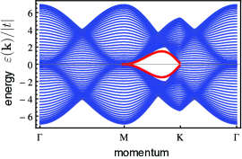
Figure 3: (color online). Surface-state spectrum projected in the Brillouin zone of the triangular lattice for (111) surface. The dispersion of the surface states corresponds to the thick red line between points M and K.

The low-temperature thermodynamic properties are governed by the density of states $\rho(\varepsilon)\propto\sqrt{\varepsilon}$ of the Majorana fermions, which is due to the quadratic band touching point. It follows that the QSL has heat capacity $C\propto T^{3/2}$, magnetic susceptibility $\chi\propto T^{1/2}$, and thermal conductivity $\kappa\propto T^{3/2}$ for $k_{B}T\ll J$. Another important property is the correlation function $G(\mathbf{r})={\langle\mathbf{J}_{j}\cdot\mathbf{J}_{j+\mathbf{r}}\rangle}$. We find that $G(\mathbf{r})$ vanishes when $\mathbf{r}$ connects sites on the same sublattice. For vectors connecting different sublattices along (100) directions in the form $\mathbf{r}=\bm{\delta}+r\hat{\mathbf{e}}$, where $\bm{\delta}\in\{(\frac{1}{2},\frac{1}{2},0),(\frac{1}{2},0,\frac{1}{2}),(0,\frac{1}{2},\frac{1}{2})\}$ and $\hat{\mathbf{e}}\in\{\hat{x},\hat{y},\hat{z}\}$, the correlation decays at large distances as $G(\mathbf{r})\sim 1/r^{4}$. This power-law decay coincides with the result for a Dirac point in two dimensions Wang and Vishwanath (2009).

Finally, we address the comparison with available experimental results for the spin liquid candidate Ba₂YMoO₆. Aharen et al. Aharen et al. (2010) observed that both the heat capacity and the magnetic susceptibility vanishes at low temperatures and have attributed this behavior to a gapped collective spin singlet. de Vries et al. de Vries, Mclaughlin, and Bos (2010) proposed a picture of a valence bond glass, but noted that the muon spin relaxation is comparable to that of QSLs de Vries et al. (2013). Here we propose that an alternative explanation for the vanishing heat capacity and susceptibility at low temperatures is the vanishing density of states of our gapless spin-orbital liquid with nodal lines. A comprehensive study of the properties of this QSL in comparison with experimental results will be presented elsewhere Nat .

To summarize, we have studied a realistic model for double perovskites in the regime of strong spin-orbit coupling. We proposed a new spin liquid ansatz that gives rise to nodal lines in the spectrum of Majorana fermions. We argued that some experimental results for Ba₂YMoO₆ can be interpreted in terms of the vanishing density of states predicted by our theory. We hope this work will stimulate the search for strongly correlated materials hosting fractional excitations with nontrivial momentum-space topology Hermanns, O’Brien, and Trebst (2015); Maciejko and Fiete (2015).

Appendix A Supplemental Material

Supplemental Material for “Chiral spin-orbital liquids with nodal lines”

W. M. H. Natori E. C. Andrade E. Miranda R. G. Pereira

Appendix B 1. Symmetry of the spin liquid ansatz

Time reversal $T=Ke^{-i\pi J^{y}_{\text{tot}}}=K\prod_{j}(i\Gamma^{13}_{j})$ acts on peudospins and pseudo-orbitals as

$$T^{-1}\mathbf{s}_{j}T=\mathbf{s}_{j},\qquad T^{-1}\tau^{x,z}_{j}T=\tau^{x,z},\qquad T^{-1}\tau^{y}_{j}T=-\tau_{j}^{y}.$$ (11)

In the Majorana fermion representation for $\mathbf{s}$ and $\bm{\tau}$ this transformation can be implemented by $T=K\prod_{j}\theta^{1}_{j}\theta^{3}_{j}$. This is equivalent to complex conjugation combined with the operation $\theta^{1}_{j}\to-\theta_{j}^{1}$ and $\theta^{3}_{j}\to-\theta^{3}_{j}$. Thus, if we focus on the decoupled flavors $\gamma\in\{\eta^{a},\theta^{2}\}$, we can take time reversal to be represented simply by complex conjugation.

Let $\gamma_{j\ell}$ denote a Majorana fermion on site $j$ belonging to sublattice $\ell=\text{A,B,C,D}$. The operators $\gamma_{\mathbf{k}\ell}$ in momentum space are defined by

$$\gamma_{j\ell} = \sqrt{\frac{8}{N}}\sum_{\mathbf{k}\in\frac{1}{2}\text{BZ}}[\gamma^{\phantom{\dagger}}_{\mathbf{k}\ell}e^{i\mathbf{k}\cdot\mathbf{R}_{j}}+\gamma^{\dagger}_{\mathbf{k}\ell}e^{-i\mathbf{k}\cdot\mathbf{R}_{j}}],$$ (12)

$$\gamma_{\mathbf{k}\ell} = \sqrt{\frac{2}{N}}\sum_{j\in\ell}\gamma_{j\ell}e^{-i\mathbf{k}\cdot\mathbf{R}_{j}},$$ (13)

and $\gamma_{\mathbf{k}\ell}$ are normalized such that $\{\gamma^{\phantom{\dagger}}_{\mathbf{k}\ell},\gamma^{\dagger}_{\mathbf{k}^{\prime}\ell^{\prime}}\}=\delta_{\mathbf{k}\mathbf{k}^{\prime}}\delta_{\ell\ell^{\prime}}$. For each flavor of Majorana fermion we combine the four sublattice modes into a single “spinor” $\gamma_{\mathbf{k}}=(\gamma_{\mathbf{k}\text{A}},\gamma_{\mathbf{k}\text{B}},\gamma_{\mathbf{k}\text{C}},\gamma_{\mathbf{k}\text{D}})^{t}$.

In momentum space, time reversal takes $\mathbf{k}\to-\mathbf{k}$. Up to a hopping amplitude (determined by self-consistent equations, see next section), the mean-field Hamiltonian for a decoupled flavor is of the form $\tilde{H}_{\text{MF}}=\sum_{\mathbf{k}\in\frac{1}{2}\text{BZ}}\gamma^{\dagger}_{\mathbf{k}}\mathcal{H}(\mathbf{k})\gamma^{\phantom{\dagger}}_{\mathbf{k}}$ with

$$\mathcal{H}({\mathbf{k}})=i\left(\begin{array}[]{cccc}0&f(k_{x},k_{y})&f(k_{y},k_{z})&f(k_{x},k_{z})\\ -f(k_{x},k_{y})&0&-f(k_{x},k_{z})&f(k_{y},k_{z})\\ -f(k_{y},k_{z})&f(k_{x},k_{z})&0&-f(k_{x},k_{y})\\ -f(k_{x},k_{z})&-f(k_{y},k_{z})&f(k_{x},k_{y})&0\\ \end{array}\right),$$ (14)

where $f(k_{a},k_{b})=4\cos(k_{a}/2)\cos(k_{b}/2)$. Notice the factor of $i$. It follows that

$$T^{-1}\mathcal{H}(\mathbf{k})T=\mathcal{H}^{*}(-\mathbf{k})=-\mathcal{H}(\mathbf{k}).$$ (15)

We define inversion $P$ as the reflection by the mirror plane that exchanges A and C sublattices (plane perpendicular to $\bm{\delta}_{yz}=(0,\frac{1}{2},\frac{1}{2})$). In momentum space, $P:k_{x}\to k_{x},k_{y}\to-k_{z},k_{z}\to-k_{y}$. In addition, we have the action in the internal (sublattice) space given by the matrix (with determinant -1)

$$P=\left(\begin{array}[]{cccc}0&0&1&0\\ 0&1&0&0\\ 1&0&0&0\\ 0&0&0&1\end{array}\right).$$ (16)

We also define the Z₂ gauge transformation that changes the sign of fermions on the B sublattice:

$$G_{P}=\left(\begin{array}[]{cccc}1&0&0&0\\ 0&-1&0&0\\ 0&0&1&0\\ 0&0&0&1\end{array}\right).$$ (17)

It is easy to check that inversion anticommutes with the mean-field Hamiltonian:

$$(PG_{P})^{-1}\mathcal{H}(P\mathbf{k})PG_{P}=-\mathcal{H}(\mathbf{k}).$$ (18)

It follows that the combined transformation $PTG_{P}$ is a symmetry of the Hamiltonian:

$$(PTG_{P})^{-1}\mathcal{H}(P\mathbf{k})PTG_{P}=\mathcal{H}(\mathbf{k}).$$ (19)

The C₃ rotation about a $(111)$ axis that leaves an A site invariant is represented by

$$C_{3}=\left(\begin{array}[]{cccc}1&0&0&0\\ 0&0&0&1\\ 0&1&0&0\\ 0&0&1&0\end{array}\right),$$ (20)

and the rotation in momentum space takes $R_{3}:k_{x}\to k_{z},k_{y}\to k_{x},k_{z}\to k_{y}$. In this case a gauge transformation is not required; we obtain immediately that

$$C_{3}^{-1}\mathcal{H}(R_{3}\mathbf{k})C_{3}=\mathcal{H}(\mathbf{k}).$$ (21)

The C₂ rotation along the $z$ axis that exchanges A$\leftrightarrow$B, C$\leftrightarrow$ D is represented by

$$C_{2}=\left(\begin{array}[]{cccc}0&1&0&0\\ 1&0&0&0\\ 0&0&0&1\\ 0&0&1&0\end{array}\right),$$ (22)

and in momentum space $R_{2}:k_{x}\to-k_{x},k_{y}\to-k_{y}$. We need to combine the C₂ rotation with the gauge transformation

$$G_{2}=\left(\begin{array}[]{cccc}1&0&0&0\\ 0&-1&0&0\\ 0&0&1&0\\ 0&0&0&-1\end{array}\right).$$ (23)

We then have

$$(C_{2}G_{2})^{-1}\mathcal{H}(R_{2}\mathbf{k})(C_{2}G_{2})=\mathcal{H}(\mathbf{k}).$$ (24)

Translation by $\bm{\delta}_{xy}=(\frac{1}{2},\frac{1}{2},0)$, which we denote by $T_{xy}$, has the same effect of exchanging sublattices as the above C₂ rotation. Thus, conjugation by $T_{xy}G_{2}$, together with $\mathbf{R}_{j}\to\mathbf{R}_{j}+\bm{\delta}_{xy}$ in real space, is also a symmetry of the Hamiltonian (and likewise for the equivalent translations in $yz$ and $xz$ planes).

Now consider a C₄ rotation along the $z$ axis going through an A site, which exchanges C and D sublattices. This can be represented in sublattice space by

$$\hat{C}_{4}=\left(\begin{array}[]{cccc}1&0&0&0\\ 0&1&0&0\\ 0&0&0&-1\\ 0&0&1&0\end{array}\right).$$ (25)

In momentum space, $R_{4}:k_{x}\to k_{y},k_{y}\to-k_{x}$. Combining with the gauge transformation:

$$\hat{G}_{4}=\left(\begin{array}[]{cccc}1&0&0&0\\ 0&-1&0&0\\ 0&0&-1&0\\ 0&0&0&1\end{array}\right),$$ (26)

we find

$$(C_{4}G_{4})^{-1}\mathcal{H}(R_{4}\mathbf{k})(C_{4}G_{4})=-\mathcal{H}(\mathbf{k}).$$ (27)

Thus, like $P$ and $T$, the C₄ rotation inverts the chirality of the ansatz. It is then easy to see that $C_{4}G_{4}T$ is a symmetry of the Hamiltonian.

The C₄ rotation can be used to construct a symmetry transformation that accounts for the twofold degeneracy of the Majorana fermion bands.

It is also interesting to consider the C₄ rotation that exchanges A and B sublattices, given by

$$\hat{C}_{4}^{\prime}=\left(\begin{array}[]{cccc}0&-1&0&0\\ 1&0&0&0\\ 0&0&1&0\\ 0&0&0&1\end{array}\right).$$ (28)

If we define this to be a rotation around $z$ axis in the opposite direction than the one in Eq. (25), the transformation in momentum space is $R_{4}^{\prime}=(R_{4})^{-1}$, i.e., $R_{4}^{\prime}:k_{x}\to-k_{y},k_{y}\to k_{x}$. It is easy to check that the composition $M=\hat{C}_{4}\hat{C}_{4}^{\prime}$ commutes with the Hamiltonian, $M^{-1}\mathcal{H}(\mathbf{k})M=\mathcal{H}(\mathbf{k})$, and obeys $M^{2}=-\mathbbm{1}$. Thus, we can block diagonalize $\mathcal{H}(\mathbf{k})$ by sectors labeled by the eigenvalue $\pm i$ of the matrix $M$:

$$U_{M}^{\dagger}\mathcal{H}(\mathbf{k})U_{M}^{\phantom{\dagger}}=\left(\begin{array}[]{cc}\tilde{\bm{\sigma}}\cdot\mathbf{h}_{\mathbf{k}}&0\\ 0&-\tilde{\bm{\sigma}}\cdot\mathbf{h}_{\mathbf{k}}\end{array}\right),$$ (29)

where $\tilde{\bm{\sigma}}\equiv(-\sigma^{z},\sigma^{y},\sigma^{x})$ and $U_{M}$ is the unitary matrix that diagonalizes $M$. It is then clear that the spectrum of $\mathcal{H}(\mathbf{k})$ is twofold degenerate with eigenvalues $\pm|\mathbf{h}_{\mathbf{k}}|$. Two degenerate states can be distinguished by the eigenvalue $\pm 1$ of the Hermitean matrix $iM$ (which is analogous to the chirality of Weyl fermions in the massless Dirac equation).

In summary, the chiral spin-orbital liquid ansatz lowers the symmetry of the Hamiltonian from O${}_{\text{h}}\times$Z₂ (where Z₂ is time reversal) to O${}_{\text{h}}$ (where the new group contains combinations of broken point group symmetries with the broken time reversal).

Appendix C 2. Berry connection

The nodal lines can be characterized as topological defects of a Berry connection in reciprocal space. In our case, the Berry connection has to be non-Abelian due to the double degeneracy of the bands. Away from the nodal lines, we define the SU(2) connection

$$A^{a}_{mn}(\textbf{k})=i\langle\psi_{m}(\textbf{k})|\partial_{k_{a}}\psi_{n}(\textbf{k})\rangle,$$ (30)

where $|\psi_{m}(\textbf{k})\rangle$ and $|\psi_{n}(\textbf{k})\rangle$, $m,n\in\{1,2\}$, are degenerate eigenstates of $\mathcal{H}(\mathbf{k})$ (say with energy $\varepsilon_{+}(\mathbf{k})$) chosen so as to obey $\langle\psi_{m}(\mathbf{k})|\psi_{n}(\mathbf{k})\rangle=\delta_{mn}$ and to diagonalize $A^{z}(\mathbf{k})$. The generalized Berry phase is the Wilson loop

$$U=\mathcal{P}\exp[-i\oint dk_{a}A^{a}(\mathbf{k})],$$ (31)

where $\mathcal{P}$ denotes path ordering. The calculation of $U$ is simplified if we consider a path around the line node parametrized by $\mathbf{k}\approx(\pi+\epsilon\cos\alpha,\pi+\epsilon\sin\alpha,k_{z})$, with $\alpha\in[-\pi,\pi)$. For infinitesimal radius $\epsilon\ll 1$, we obtain

$$A^{x}=-\frac{1}{2\epsilon}\sin\alpha\,\sigma^{y}+\mathcal{O}(\epsilon^{0}),\qquad A^{y}=\frac{1}{2\epsilon}\cos\alpha\,\sigma^{y}+\mathcal{O}(\epsilon^{0}),$$ (32)

which is precisely the singular $\epsilon$ dependence of a vortex line. We then find $U=-\mathbbm{1}$, equivalent to a $\pi$ Berry phase.

Appendix D 3. Solving the mean-field Hamiltonian

In this section we outline the steps required to diagonalize the mean-field Hamiltonian and calculate the ground state energy.

Using the mode expansion Eq. (12), we can rewrite the various hopping terms for Majorana fermions in terms of operators in reciprocal space. For instance,

$$i\sum_{\langle j,l\rangle\in\text{XY}}\gamma_{j\text{A}}\gamma_{l\text{B}}=2i\sum_{\mathbf{k}\in\frac{1}{2}\text{BZ}}h_{\mathbf{k}}^{1}(\gamma^{\dagger}_{\mathbf{k}\text{A}}\gamma^{\phantom{\dagger}}_{\mathbf{k}\text{B}}-\gamma^{\dagger}_{\mathbf{k}\text{B}}\gamma^{\phantom{\dagger}}_{\mathbf{k}\text{A}}),$$ (33)

where $h_{\mathbf{k}}^{1}=4\cos(k_{x}/2)\cos(k_{y}/2)$ is the first component of $\mathbf{h}_{\mathbf{k}}$. The mean-field Hamiltonian becomes

$$\tilde{H}_{\text{MF}} = \frac{J}{18}\sum_{\textbf{k}\in\frac{1}{2}\text{BZ}}\left[(2u+\bar{w})\sum_{a=1}^{3}\left(\eta^{a}_{\textbf{k}}\right)^{\dagger}\mathcal{H}_{1}(\mathbf{k})\eta_{\textbf{k}}^{a}-w\left(\theta_{\textbf{k}}^{2}\right)^{\dagger}\mathcal{H}_{1}(\mathbf{k})\theta_{\textbf{k}}^{2}+\left(\Theta_{\textbf{k}}\right)^{\dagger}\mathcal{H}_{2}(\mathbf{k})\Theta_{\mathbf{k}}\right]$$ (34)

$$-\frac{NJ}{6}+\frac{J}{36}\underset{\langle i,j\rangle\in\alpha}{\sum}\left(3u_{ij}^{2}+3\bar{w}^{\alpha}_{ij}u_{ij}-w^{\alpha}_{ij}v_{ij}\right),$$

where $\mathcal{H}_{1}(\mathbf{k})$ is the $4\times 4$ matrix in Eq. (14), $\Theta_{\mathbf{k}}=(\theta^{1}_{\mathbf{k}\text{A}},\dots,\theta^{3}_{\mathbf{k}\text{D}})^{t}$ is an eight-component spinor that combines $\theta^{1}$ and $\theta^{3}$ fermions and $\mathcal{H}_{2}(\mathbf{k})$ is an $8\times 8$ matrix to be specified below.

First consider the fermions $\zeta\in\{\eta^{a},\theta^{2}\}$, whose spectrum is determined by $\mathcal{H}_{1}(\mathbf{k})$. Let $U_{\textbf{k}}$ be the unitary transformation that diagonalizes $\mathcal{H}_{1}(\mathbf{k})$:

$$U^{\dagger}_{\mathbf{k}}\mathcal{H}_{1}(\mathbf{k})U_{\mathbf{k}}^{\phantom{\dagger}}=\Lambda_{1}({\mathbf{k}}),$$ (35)

where $\Lambda_{1}({\mathbf{k}})=\text{diag}\{-|\mathbf{h}_{\mathbf{k}}|,-|\mathbf{h}_{\mathbf{k}}|,|\mathbf{h}_{\mathbf{k}}|,|\mathbf{h}_{\mathbf{k}}|\}$ is a diagonal matrix. The operators that annihilate fermions in eigenstates of $\mathcal{H}_{1}(\mathbf{k})$ are

$$\tilde{\gamma}_{\mathbf{k}\lambda} = \sum_{\ell=\text{A},\dots,\text{D}}(U^{\dagger})_{\lambda\ell}\gamma_{\mathbf{k}\ell},$$ (36)

$$\gamma_{\mathbf{k}\ell} = \sum_{\lambda=1}^{4}(U)_{\ell\lambda}\tilde{\gamma}_{\mathbf{k}\lambda},$$ (37)

where $\lambda=1,\dots,4$ is the band index. The mean-field ground state $|\text{GS}\rangle$ is the state in which all single-fermion states with negative energy are occupied. This leads to the self-consistent equation for expectation values, e.g.

$$\langle\gamma_{j,\text{A}}\gamma_{j+\bm{\delta}_{xy},\text{B}}\rangle = \frac{8}{N}\sum_{\mathbf{k}\in\frac{1}{2}\text{BZ}}[e^{i\mathbf{k}\cdot\bm{\delta}_{xy}}\langle\gamma^{\dagger}_{\mathbf{k}\text{A}}\gamma^{\phantom{\dagger}}_{\mathbf{k}\text{B}}\rangle+e^{-i\mathbf{k}\cdot\bm{\delta}_{xy}}\langle\gamma^{\phantom{\dagger}}_{\mathbf{k}\text{A}}\gamma^{\dagger}_{\mathbf{k}\text{B}}\rangle]$$ (38)

$$= i\text{Im}\left[\frac{16}{N}\sum_{\mathbf{k}\in\frac{1}{2}\text{BZ}}\sum_{\lambda}(U^{\dagger})_{\lambda\text{A}}U_{\text{B}\lambda}e^{i\mathbf{k}\cdot\bm{\delta}_{xy}}\langle\tilde{\gamma}^{\dagger}_{\mathbf{k}\lambda}\tilde{\gamma}^{\phantom{\dagger}}_{\mathbf{k}\lambda}\rangle\right]$$

$$= \frac{i}{2\pi^{3}}\text{Im}\left\{\sum_{\lambda\,(\epsilon_{\lambda}<0)}\int_{\frac{1}{2}\text{BZ}}d^{3}k\,(U^{\dagger})_{\lambda\text{A}}U_{\text{B}\lambda}\right\},$$

where in the last line the sum is over bands with negative energy and we took the thermodynamic limit to replace $\sum_{\mathbf{k}}\to\frac{N}{32\pi^{3}}\int d^{3}k$ (corresponding to $N/4$ states in the Brillouin zone of the cubic sublattice).

Since $\mathcal{H}_{1}(\mathbf{k})$ determines the spectrum of $\eta^{a}$ and $\theta^{2}$ fermions, the self-consistent equations for $u_{ij}=-i\langle\eta_{i}^{a}\eta_{j}^{a}\rangle$ and $v_{ij}=-i\langle\theta_{i}^{2}\theta_{j}^{2}\rangle$ are the same up to an overall minus sign, depending on the relative sign of the hopping amplitudes $2u+\bar{w}$ and $-w$ in Eq. (34) We then have the constraint $|u|=|v|$, but must analyze two possibilities, namely $u=v$ and $u=-v$. Without loss of generality (by choosing one of the two degenerate ground states with opposite chiralities), we can set $u>0$. Numerical evaluation of the integral in Eq. (38) then yields $u\approx 0.258$.

The relation between $u$ and $v$ determines the $8\times 8$ matrix for $\Theta_{\mathbf{k}}$. For $v=u$, we obtain

$$\mathcal{H}_{2}(\textbf{k})=u\textbf{h}_{\textbf{k}}\cdot\bm{\Sigma}^{\prime},$$ (39)

where $\bm{\Sigma}^{\prime}=\left(2K^{z}\otimes\sigma^{y},-2K^{y}\otimes\mathbbm{1},-2K^{x}\otimes\sigma^{y}\right)$, with

$$K^{x}=\frac{1}{2}\left(\begin{array}[]{cccc}0&2&0&\sqrt{3}\\ 2&0&\sqrt{3}&0\\ 0&\sqrt{3}&0&0\\ \sqrt{3}&0&0&0\end{array}\right),\quad K^{y}=\frac{i}{2}\left(\begin{array}[]{cccc}0&-2&0&\sqrt{3}\\ 2&0&-\sqrt{3}&0\\ 0&\sqrt{3}&0&0\\ -\sqrt{3}&0&0&0\end{array}\right),\quad K^{z}=\frac{1}{2}\left(\begin{array}[]{cccc}1\\ &-1\\ &&-3\\ &&&3\end{array}\right).$$ (40)

The components of the matrix vector $\mathbf{K}$ satisfy the SU(2) algebra. We then obtain the spectrum of $\mathcal{H}_{2}(\mathbf{k})$ and use it to solve the self-consistent equations for $w_{ij}=-i\langle\theta_{i}^{\alpha}\theta_{j}^{\alpha}\rangle$ and $\bar{w}_{ij}=-i\langle\bar{\theta}_{i}^{\alpha}\bar{\theta}_{j}^{\alpha}\rangle$ analogous to Eq. (38). In this case of $u=v$ we find a self-consistent solution with $w\approx-0.081$ and $\bar{w}\approx 0.317$. Having fixed the order parameters, we obtain the mean-field ground states energy $E_{\text{MF}}(v=u)=\langle\tilde{H}_{\text{MF}}\rangle\approx-0.244NJ$.

For $v=-u$ we obtain

$$H_{\textbf{k}}^{(2)}=u\textbf{h}_{\textbf{k}}\cdot\bm{\Sigma}^{\prime\prime},$$ (41)

where $\bm{\Sigma}^{\prime\prime}=\left(\left(2-\sigma^{xy}\right)\otimes\Sigma^{1},\left(2-\sigma^{yz}\right)\otimes\Sigma^{2},\left(2-\sigma^{xz}\right)\otimes\Sigma^{3}\right)$, with $\bm{\Sigma}$ the matrix vector defined in the main text, and the $2\times 2$ matrices $\sigma^{\alpha}$ given by $\sigma^{xy}=\sigma^{z}$, $\sigma^{yz(xz)}=\frac{1}{2}(-\sigma^{z}\pm\sqrt{3}\sigma^{x})$. In this case we find a self-consistent solution with $w\approx 0.161$ and $\bar{w}\approx 0.318$. The ground state energy is $E_{\text{MF}}(v=-u)\approx-0.248NJ$, slightly lower than the result for $u=v$. This is the value quoted in the main text. We note that the small difference between the two energies may change beyond the mean-field level. However, we have verified that both solutions give rise to a spectrum with nodal lines along MR directions, qualitatively similar to the spectrum for $\eta^{a}$ and $\theta^{2}$ fermions. Therefore, the properties derived from the low-energy density of states $\rho(\epsilon)\propto\sqrt{\epsilon}$ are generic.

Appendix E 4. Variational Monte Carlo

To check the viability of the proposed chiral spin-orbital liquid beyond the mean-field level, we now enforce the local constraint exactly by considering a Gutzwiller projection of the mean-field wave function (Gros, 1989) by means of a variational Monte Carlo calculation (Ceperley, Chester, and Kalos, 1977).

We begin by rewriting the Majorana fermions in terms of three Dirac fermions, closely following the representation used in Ref. (Wang and Vishwanath, 2009)

$$c_{i}^{\dagger}=\frac{1}{2}\left(\eta_{i}^{2}+i\theta_{i}^{2}\right),\;d_{i}^{\dagger}=\frac{1}{2}\left(\eta_{i}^{1}+i\eta_{i}^{3}\right),\;f_{i}^{\dagger}=\frac{1}{2}\left(\theta_{i}^{1}+i\theta_{i}^{3}\right).$$ (42)

In terms of this representation, the local constraint is now translated into the fact that a given site may either have no Dirac fermions, a state denoted by $\left|0\right\rangle$, or two Dirac fermions, in which case there are three possible states at each site defined as

$$\left|x_{i}\right\rangle=c_{i}^{\dagger}d_{i}^{\dagger}\left|0\right\rangle,\;\left|y_{i}\right\rangle=d_{i}^{\dagger}f_{i}^{\dagger}\left|0\right\rangle,\;\left|z_{i}\right\rangle=f_{i}^{\dagger}c_{i}^{\dagger}\left|0\right\rangle.$$ (43)

Given a real space configuration specified by the locations of the doubly occupied sites, $X\equiv\left\{x_{i}\right\},Y\equiv\left\{y_{i}\right\},Z\equiv\left\{z_{i}\right\}$, the wave function assigns an amplitude $\Psi\left(\left\{x_{i}\right\},\left\{y_{j}\right\},\left\{z_{m}\right\}\right)$ to it. Notice that the locations of the $\left|0\right\rangle$ states are automatically specified. We point out that the local constraint only fixes the parity of the number of fermions but not the number itself. Moreover, our Hamiltonian contains terms which not only create/annihilate two particles, e.g. $\left|x_{i}\right\rangle\leftrightarrows\left|0\right\rangle$, but also terms which preserve the total number of fermions while changing the number of each of the three individual fermionic flavors, e.g. $\left|x_{i}\right\rangle\leftrightarrows\left|y_{i}\right\rangle$. Although it is possible to write down a projected wave functions with varying particle number (Edegger et al., 2005), we refrain from doing so in this work for the sake of computational simplicity. Instead, we consider a restrictive form for the ground state wave function: each one of the four states is equally distributed over $N/4$ distinct sites, with $\left\{x_{i}\right\}=\left\{x_{1},x_{2},\ldots,x_{N/4}\right\}$, etc.

The mean-field Hamiltonian in the main text may be rewritten, in terms of the three Dirac fermions in Eq. (42), as

$$\mathcal{H}_{MF} = -\frac{NJ}{6}+\frac{J}{36}\sum_{\left\langle jl\right\rangle\in\alpha}\left[\left(3u_{jl}^{2}+3\bar{w}_{jl}^{\alpha}u_{jl}-w_{jl}^{\alpha}v_{jl}\right)+i\left(4u_{jl}+2\bar{w}_{jl}^{\alpha}\right)d_{j}^{\dagger}d_{l}\right.$$ (44)

$$+\left.i\left(2u_{jl}+\bar{w}_{jl}^{\alpha}-w_{jl}^{\alpha}\right)c_{j}^{\dagger}c_{l}+i\left(2u_{jl}+\bar{w}_{jl}^{\alpha}+w_{jl}^{\alpha}\right)c_{j}^{\dagger}c_{l}^{\dagger}+i\left(3u_{jl}-v_{jl}\right)f_{j}^{\dagger}f_{l}+\mbox{h.c.}\right]$$

$$-\frac{J}{36}\sum_{\left\langle jl\right\rangle\in XY}\left[i\left(3u_{jl}+v_{jl}\right)f_{j}^{\dagger}f_{l}^{\dagger}+\mbox{h.c.}\right]+\frac{J}{36}\sum_{\left\langle jl\right\rangle\in YZ}\left[i\left(3u_{jl}e^{i\pi/3}+v_{jl}e^{-2i\pi/3}\right)f_{j}^{\dagger}f_{l}^{\dagger}+\mbox{h.c.}\right]$$

$$+\frac{J}{36}\sum_{\left\langle jl\right\rangle\in XZ}\left[i\left(3u_{jl}e^{i\pi/3}-v_{jl}e^{-2i\pi/3}\right)f_{j}^{\dagger}f_{l}^{\dagger}+\mbox{h.c.}\right].$$

The three fermion flavors are decoupled and we may thus write the mean-field wave function as a product of three Slater determinants. Thus, after the Gutzwiller projection, we obtain

$$\Psi\left(\left\{x_{i}\right\},\left\{y_{j}\right\},\left\{z_{m}\right\}\right)= \Phi_{d}\left(\left\{x_{i}\right\},\left\{y_{j}\right\}\right)\cdot\Phi_{f}\left(\left\{y_{j}\right\},\left\{z_{m}\right\}\right)\cdot \Phi_{c}\left(\left\{z_{m}\right\},\left\{x_{i}\right\}\right).$$ (45)

The $d$-fermion sector of the Hamiltonian in Eq. (44) corresponds to free fermions and thus their mean-field ground state is obtained by filling up the states with negative energy. For the $c$ and $f$-fermions we have a BCS-like Hamiltonian instead and their ground state is given by the vacuum of their respective Bogoliubov quasiparticles (Gros, 1989). The different status of the $d$ fermion is expected from symmetry: the hidden global SU(2) symmetry of the original Hamiltonian implies the global U(1) symmetry corresponding to the conservation of the total number of Dirac fermions defined by a combination of $\eta$ Majorana fermions. On the other hand, there is no continuous symmetry associated with $\theta$ Majorana fermions; as a result, the total number of $c$ and $f$ fermions is not conserved. The need to work with BCS-type wave functions in our case should be contrasted with the case of SU(4) symmetric models Wang and Vishwanath (2009), where the SU(4) symmetry implies the conservation of the numbers of all three flavors of Dirac fermions.

After constructing the mean-field wave function, we then implemented a variational Monte Carlo calculation of the Gutzwiller-projected ground state energy $E^{\text{VMC}}_{\text{gs}}$. We started by generating an initial state in which we populate $N/4$ randomly chosen sites with the $x$-state $\left(\left\{x_{i}\right\}\right)$, then $N/4$ of the remaining sites with the $y$-state $\left(\left\{y_{i}\right\}\right)$, and finally $N/4$ of the further remaining sites with the $z$-state $\left(\left\{z_{i}\right\}\right)$. Our Monte Carlo moves consist in exchanging random pairs of sites containing distinct states. We allow for moves involving widely separated sites — and which would not be connected by the Hamiltonian — because this improves the sampling over the space of configurations. We accept or reject these moves according to the usual Metropolis algorithm. After $N$ such exchange attempts, we are said to have performed one Monte Carlo sweep and after every sweep we compute $E^{\text{VMC}}_{\text{gs}}$. $N_{\mbox{warm}}$ sweeps are performed before measurements of physical quantities for “thermalization”. Averages are then performed over $N_{\mbox{sweep}}$ sweeps. We typically considered $N_{\mbox{warm}}=N_{\mbox{sweep}}\sim 10^{4}$. The results were obtained for lattices of size $N=4L^{3}$ with $L=4$, $6$, and $8$. We find that the change in the ground state energy with $N$ is smaller than the Monte Carlo error bars for the system sizes considered here. Thus, we quote the results for $L=8$ as the converged ones.

We computed the ground state energy for the two sets of mean-field parameters quoted in this supplemental material. For $u=v=0.258$, $\bar{w}=0.317$, and $w=-0.081$ we obtain $E^{\text{VMC}}_{\text{gs}}=-0.39\left(1\right)NJ$. As for $u=-v=0.258$, $\bar{w}=0.318$, and $w=0.161$ we obtain $E^{\text{VMC}}_{\text{gs}}=-0.40\left(1\right)NJ$. Clearly, the Gutzwiller projection decreases significantly the mean-field energy down to values which are already comparable to that obtained, for instance, for a valence-bond covering of the lattice $\left(E_{\text{VBS}}=-0.417NJ\right)$ (Chen, Pereira, and Balents, 2010), thus showing that the proposed chiral spin-orbital liquid is a competitive ground state candidate.

In light of this favorable energy of our proposed ansatz, we conclude by pointing out two important restrictions in our variational Monte Carlo calculation that, once lifted, should further decrease the value of the ground state energy $E^{\text{VMC}}_{\text{gs}}$:

1. For the quoted values of $E^{\text{VMC}}_{\text{gs}}$, we considered the optimal values for the mean-field amplitudes $v$, $\bar{w}$ and $w$ obtained before the Gutzwiller projection, i.e., at the mean-field level;

2. The restrictive form of the considered wave function neglects variations both in the populations of the fermionic flavors and in the total number of fermions.

We stress that these restrictions were important for this first calculation beyond mean field due to the complexity of the chiral spin-orbital liquid ansatz considered here. We leave a more detailed investigation, together with a more precise estimate for the variational energy of our spin liquid ansatz, for future work.