Direct Variational Perspective Shape from Shading with Cartesian Depth Parametrisation

Abstract

Most of today’s state-of-the-art methods for perspective shape from shading are modelled in terms of partial differential equations (PDEs) of Hamilton-Jacobi type. To improve the robustness of such methods w.r.t. noise and missing data, first approaches have recently been proposed that seek to embed the underlying PDE into a variational framework with data and smoothness term. So far, however, such methods either make use of a radial depth parametrisation that makes the regularisation hard to interpret from a geometrical viewpoint or they consider indirect smoothness terms that require additional consistency constraints to provide valid solutions. Moreover the minimisation of such frameworks is an intricate task, since the underlying energy is typically non-convex. In this chapter we address all three of the aforementioned issues. First, we propose a novel variational model that operates directly on the Cartesian depth. In contrast to existing variational methods for perspective shape from shading this refers to both the data and the smoothness term. Moreover, we employ a direct second-order regulariser with edge-preservation property. This direct regulariser yields by construction valid solutions without requiring additional consistency constraints. Finally, we also propose a novel coarse-to-fine minimisation framework based on an alternating explicit scheme. This framework allows us to avoid local minima during the minimisation and thus to improve the accuracy of the reconstruction. Experiments show the good quality of our model as well as the usefulness of the proposed numerical scheme.

1 Introduction

Shape from Shading (SfS) is a classic task in computer vision. Given information on light reflectance and illumination in a photographed scene, the aim of SfS is to compute based on the brightness variation the 3D structure of a depicted object from a single input image. SfS has a wide variety of applications, ranging from large scale problems such as astronomy Rindfleisch1966 or terrain reconstruction Bors_TPAMI2003 to small scale tasks such as dentistry Abdelrahim_BMVC2011 or endoscopy Okatani_CVIU1997 ; Wang_MST2009 ; Wu_IJCV2010 .

Classical Methods. First approaches to SfS go back to 1951 and 1966, respectively, when Van Diggelen VanDiggelen1951 and Rindfleisch Rindfleisch1966 used SfS techniques to reconstruct the surface of the moon. Later on in the 1970’s, Horn Ho70 was the first one to tackle the SfS problem by solving a partial differential equation (PDE) approach. In 1981, he and Ikeuchi were also the first ones to model the SfS problem using a variational framework Ikeuchi_AI1981 . The most prominent classical variational approach is given by the work of Horn and Brooks HB86 . Assuming a simple orthographic projection model, a light source at infinity as well as a Lambertian reflectance model, they proposed to compute the normals of the unknown surface as minimiser of an energy functional.

Those first approaches, however, had several drawbacks. The model assumptions were very simple and mainly suitable in the context of astronomical applications. In fact, the use of an orthographic projection model with a light source located at infinity requires the distances between camera, light source and illuminated object to be huge. Also the depth was not estimated directly such that the SfS process required a postprocessing step that performed a numerical integration of the estimated surface normals. Thereby, inconsistent gradient fields turned out to be a problem, so that extensions of the original model were required that tried to enforce this consistency during or after the estimation Frankot_TPAMI1988 ; HB89 . Finally, in case of variational methods, the smoothness term was restricted to a quadratic regulariser HB86 ; Ikeuchi_AI1981 . While such standard smoothness terms simplify the minimisation of the underlying energy, they do not allow to preserve discontinuities in the depth and thus lead to oversmoothed solutions Ol91 . For a detailed review of most of the classical methods the reader is referred to DFS08 ; Ho86 ; HB89 ; ZTCS99 .

Perspective Shape from Shading. At the end of the 1990’s research mainly focused on novel concepts for formulating orthographic SfS such as viscosity solutions RouyTourin_SINUM1992 and level set formulations Kimmel_IJCV1995 . However, for most applications results were not satisfactory ZTCS99 . In the early 2000’s, the situation changed completely. Inspired by the work of Okatani and Deguchi Okatani_CVIU1997 , independently, Prados and his co-workers PF03b ; Prados_CVPR2005 as well as two other research groups CCDG04a ; TSY03 proposed to consider a perspective camera model. Evidently, such a model is particularly appropriate for tasks that require the object to be relatively close to the camera such as e.g. in medical endoscopy. In such cases the perspective effects dominate and an orthographic projection model would cause significant systematic errors as shown in TSY05 . Secondly, Prados and colleagues proposed to shift the light source location from infinity to the camera centre which can be seen as a good approximation of a camera with photoflash. This made shape from shading attractive for a variety of photo-based applications. Finally, also a physically motivated light attenuation term was introduced that models a quadratic fall-off due to the inverse square law. As discussed in BCDFV12 , the use of this term largely resolved the convex-concave ambiguity that was inherent to the classical orthographic model although some ambiguities are still present. Even the generalisation of such approaches to advanced reflectance models such as the Oren-Nayar Oren_IJCV1995 or the Phong reflectance model Phong_CACM1975 have been recently investigated AF2006 ; VBW08 .

However, this evolution of SfS models was accompanied by a different way of formulating the SfS problem. Instead of using variational methods, the perspective SfS problem was formulated in terms of hyperbolic PDEs Prados_CVPR2005 . Although such PDE formulations allow for an efficient computation of the solution using fast marching schemes Sethian1999 , they suffer from two inherent drawbacks: (i) On the one hand, they are prone to noise and missing data, since they do not rely on any form of regularisation or filling-in. This can be particularly problematic in the context of real-world images. (ii) On the other hand, it is difficult to extend the underlying model of such PDE-based schemes by additional constraints such as smoothness terms, multiple views, or additional light sources. While there have been recently some PDE-based approaches to photometric stereo MF13 , one has to take care of ensuring the uniqueness of the solution if the input data from multiple images is not consistent, cf. the discussion in Mecca_SIIMS14 .

Variational Perspective Shape from Shading. Given the flexibility and robustness of variational methods, it is not surprising that recently researchers tried to close the evolutionary loop by integrating the perspective SfS model into a suitable variational framework. So far, however, there are only a few works in the literature that deal with this recent idea. On the one hand, there is the work of Ju et al. JBB2014 that embeds the PDE of Prados et al. Prados_CVPR2005 as data term into a variational model and complements it with a discontinuity-preserving second order smoothness term. However, since the approach penalises deviations from the PDE directly and uses a parametrisation in terms of the radial depth, deviations in both the data and the smoothness term are difficult to interpret geometrically or photometrically. On the other hand, there is the approach of Abdelrahim et al. Abdelrahim_ICIP 2013 that formulates the data term in terms of brightness differences and makes use of a Cartesian depth parametrisation. While the corresponding energy functional is thus more meaningful from a geometric and photometric viewpoint, it defines smoothness based on surface normals and thus needs an additional integrability constraint. Moreover, the corresponding smoothness term is restricted to a simple homogeneous regulariser that does not allow to preserve object edges during the reconstruction. Finally, there are the works of Zhang et al. ZYT07 and Wu et al. Wu_IJCV2010 that also make use of a Cartesian depth parametrisation but rely on an indirect estimation using auxiliary variables. While the approach of Zhang et al. ZYT07 resolves the resulting consistency problem by considering an integrability constraint, the method of Wu et al. Wu_IJCV2010 repeatedly integrates the surface normals during computation to ensure valid solutions. Moreover, both approaches use derivations for their surface normals that are based on the orthographic projection model of Horn and Brooks HB89 . Unfortunately, the resulting models are thus only valid in case of weak perspective distortions.

A final issue that is common to all four of the aforementioned works is the difficulty of minimising the underlying energy. Since this energy is non-convex, two of the methods rely on initialisations provided by closely related PDE-based SfS approaches Abdelrahim_ICIP 2013 ; ZYT07 . This, however, contradicts the idea of introducing robustness into the estimation – in particular in the presence of noise or missing data. In contrast, the other two methods estimate the solution from scratch JBB2014 ; Wu_IJCV2010 . However, those methods do not provide any quantitative assessment of the reconstruction quality.

Let us summarise: While from a modelling viewpoint, it would be desirable to design a variational model that directly solves for the Cartesian depth without the need of integrability constraints or repeated integrations steps, it would be helpful from an optimisation viewpoint to develop a minimisation scheme that neither depends on the solution of other SfS techniques as in Abdelrahim_ICIP 2013 ; ZYT07 nor requires an accurate initialisation to produce meaningful results.

Our Contributions. In this book chapter we contribute to the field of variational SfS in three ways: (i) First, we consider a variational model for perspective SfS that makes use of a Cartesian depth parametrisation and an edge-preserving Cartesian depth regularisation. By penalising deviations from the image brightness in the data term and regularising the Cartesian depth in the smoothness term directly, we obtain an approach that is geometrically and photometrically meaningful. In this context, we also point out a popular mistake in the derivation of the surface normal and show two different ways to derive the normal correctly. (ii) Our method is a direct approach to depth computation, i.e. it does not yield gradient fields that need to be integrated in a subsequent step, nor do we employ integrability constraints. (iii) Apart from the novel model, we also propose a novel minimisation strategy. By embedding an alternating explicit scheme into a coarse-to-fine scheme, we obtain an optimisation framework that allows to obtain significantly better results than a traditional explicit scheme. Experiments with synthetic and real-world images show the good quality of our reconstructions and the advantages of our numerical scheme.

Organisation of the Chapter. In Section 2 we propose a novel PDE-based model for perspective SfS that is based on a Cartesian parametrisation of the depth. In Section 3 we then embed this PDE into a variational framework with appropriate second order smoothness term. Details on the minimisation and the discretisation are provided in Section 4, while Section 5 comments on the integration of intrinsic camera parameters. Finally, a detailed evaluation of our approach is presented in Section 6. The paper concludes with a summary in Section 7.

2 Perspective SfS with Cartesian Depth Parametrisation

In this section, we introduce a novel PDE-based SfS model that is parametrised in terms of the Cartesian depth. In contrast to most existing SfS models that estimate the radial depth or multiples thereof, such a Cartesian parametrisation expresses the unknown surface directly in terms of the Euclidean distance along the $z$-axis, which is the axis orthogonal to the image plane.

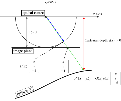
Figure 1: Relation between the radial depth factor $u(\mathbf{x})$ (quotient between green and blue distance) that denotes the depth in multiples of the focal length $\mathtt{f}$ and the Cartesian depth $z(\mathbf{x})$ (red distance).

Parametrisation of the Surface. The starting point for our new model is formed by the classical PDE-approach of Prados et al. Prados_CVPR2005 which is originally parametrised in terms of the radial depth. Key assumptions of this SfS model are that a point light source is located at the optical centre of a perspective camera and that the surface reflectance is Lambertian with uniform albedo that is fixed to one. The unknown surface $\mathcal{S}:\overline{\Omega}_{\mathbf{x}}\rightarrow\mathbb{R}^{3}$ can then be described as

$$\mathcal{S}\left(\mathbf{x},u(\mathbf{x})\right)=\left\{\dfrac{\mathtt{f}}{\sqrt{\left|\mathbf{x}\right|^{2}+\mathtt{f}^{2}}}\;u(\mathbf{x})\left[\left.\begin{array}[]{c}x\\ y\\ -\mathtt{f}\end{array}\right]\right|\;\mathbf{x}:=\left(x,y\right)^{\top}\in\overline{\Omega}_{\mathbf{x}}\right\}\,,$$ (1)

where $\mathbf{x}=(x,y)^{\top}\in\overline{\Omega}_{\mathbf{x}}$ is the position in the closure $\overline{\Omega}_{\mathbf{x}}$ of the rectangular image domain $\Omega_{\mathbf{x}}\subset\mathbb{R}^{2}$, $\mathtt{f}$ denotes the focal length of the camera and $u(\mathbf{x})$ is a multiple of $\mathtt{f}$ that describes the radial distance (depth) of the surface from the camera centre.

Since the third component in Eq. (1) corresponds to the negative Cartesian depth $z$, we can derive the following relationship to the radial depth $u\,\mathtt{f}$

$$z(\mathbf{x})=\dfrac{\mathtt{f}}{\sqrt{\left|\mathbf{x}\right|^{2}+\mathtt{f}^{2}}}\,u(\mathbf{x})\,\mathtt{f}\;\stackrel{{\scriptstyle\mbox{\tiny\eqref{eq:13}}}}{{=}}\;Q(\mathbf{x})\,u(\mathbf{x})\,\mathtt{f}\,,$$ (2)

where $Q(\mathbf{x})$ denotes a spatially variant conversion factor given by

$$Q(\mathbf{x})=\dfrac{\mathtt{f}}{\sqrt{|\mathbf{x}|^{2}+\mathtt{f}^{2}}}\,.$$ (3)

This relation is illustrated in Figure 1.

Plugging Eq. (3) into Eq. (1), we then obtain the parametrisation of the original surface $\mathcal{S}$ with respect to the Cartesian depth $z$

$$\mathcal{S}\left(\mathbf{x},z(\mathbf{x})\right)\stackrel{{\scriptstyle\mbox{\tiny\eqref{eq:13}}}}{{=}}Q(\mathbf{x})\,u(\mathbf{x})\left[\begin{array}[]{c}x\vspace{0.5ex}\\ y\vspace{0.5ex}\\ -\mathtt{f}\end{array}\right]\stackrel{{\scriptstyle\mbox{\tiny\eqref{eq:64}}}}{{=}}Q(\mathbf{x})\,\left(\dfrac{z(\mathbf{x})}{\mathtt{f}\,Q(\mathbf{x})}\right)\left[\begin{array}[]{c}x\vspace{0.5ex}\\ y\vspace{0.5ex}\\ -\mathtt{f}\end{array}\right]=\left[\begin{array}[]{c}\dfrac{z(\mathbf{x})\,x}{\mathtt{f}}\vspace{1ex}\\ \dfrac{z(\mathbf{x})\,y}{\mathtt{f}}\vspace{1ex}\\ -z(\mathbf{x})\end{array}\right]\,.$$ (4)

Brightness Equation. After we have parametrised the original surface in terms of the Cartesian depth, let us now derive the resulting brightness equation that relates the local orientation of the surface to the image brightness. Assuming a Lambertian reflectance model and a quadratic light attenuation term that follows the inverse square law, we obtain the following general brightness equation Prados_CVPR2005 :

$$I(\mathbf{x})=\dfrac{1}{r(\mathbf{x})^{2}}\left(\dfrac{\mathbf{n}(\mathbf{x})}{|\mathbf{n}(\mathbf{x})|}\cdot\mathbf{L}(\mathbf{x})\right)\,,$$ (5)

where $I$ is the recorded image, ${\mathbf{n}}$ is the surface normal vector, $\mathbf{L}$ stands for the normalised light direction vector, and $r$ is the (radial) distance of the light source to the surface. Knowing that $r=\mathtt{f}\,u$ and using Eq. (2) we can express the quadratic light attenuation term using the Cartesian depth $z$

$$r(\mathbf{x})=\mathtt{f}u(\mathbf{x})=\dfrac{z(\mathbf{x})}{Q(\mathbf{x})}\;\Rightarrow\;\;\;\;\dfrac{1}{r(\mathbf{x})^{2}}=\frac{Q(\mathbf{x})^{2}}{z(\mathbf{x})^{2}}\,.$$ (6)

What remains to be computed in terms of the Cartesian depth are the surface normal $\mathbf{n}$ and the light direction vector $\mathbf{L}$, respectively.

Surface Normal. Let us start by deriving the surface normal. Since the surface normal is the normal vector of the tangent plane, we first have to compute the partial derivatives of the surface in Eq. (4) in $x$- and $y$-direction, respectively

$$\mathcal{S}_{x}(\mathbf{x},z)=\left[\begin{array}[]{c}\dfrac{z_{x}\,x+z}{\mathtt{f}}\vspace{1ex}\\ \dfrac{z_{x}\,y}{\mathtt{f}}\vspace{1ex}\\ -z_{x}\end{array}\right]\;,\;\;\;\;\;\mathcal{S}_{y}(\mathbf{x},z)=\left[\begin{array}[]{c}\dfrac{z_{y}\,x}{\mathtt{f}}\vspace{1ex}\\ \dfrac{z_{y}\,y+z}{\mathtt{f}}\vspace{1ex}\\ -z_{y}\end{array}\right]\,.$$ (7)

Here and for the whole paper we dropped the spatial dependency of $z$, $z_{x}$ and $z_{y}$ on $\mathbf{x}$ for the sake of clarity. Taking the cross-product then yields the direction of the surface normal

$$\mathbf{n}(\mathbf{x})=\mathcal{S}_{x}(\mathbf{x},z)\times\mathcal{S}_{y}(\mathbf{x},z)=\left[\begin{array}[]{c}\dfrac{z_{x}\,z}{\mathtt{f}}\vspace{1ex}\\ \dfrac{z_{y}\,z}{\mathtt{f}}\vspace{1ex}\\ \dfrac{z\,\left[\left(\nabla z\cdot\mathbf{x}\right)+z\right]}{\mathtt{f}^{2}}\end{array}\right]\,.$$ (8)

Light Direction. Let us now turn towards the computation of the light direction. Since the light source is assumed to be located in the camera centre which coincides with the origin of the coordinate system, the direction of the light rays and the direction of the optical rays coincide (up to sign). Hence, the light direction can just be read off Eq. (1) as

$$\mathbf{L}(\mathbf{x})=\dfrac{1}{\sqrt{|\mathbf{x}|^{2}+\mathtt{f}^{2}}}\left[\begin{array}[]{c}-{x}\\ -{y}\\ \mathtt{f}\end{array}\right]\,.$$ (9)

PDE-Based Model. By plugging the surface normal from Eq. (8) and the light direction from Eq. (9) into the brightness equation (5) we finally obtain our perspective SfS model with the new Cartesian depth parametrisation

$$I-\dfrac{Q^{3}}{z\,\sqrt{\mathtt{f}^{2}\,\left|\nabla z\right|^{2}+\left[\left(\nabla z\cdot\mathbf{x}\right)+z\right]^{2}}}=0\,.$$ (10)

Here and for the whole paper we dropped the spatial dependency of $I$ and $Q$ on $\mathbf{x}$ for the sake of clarity.

The main properties of our new model (10) are naturally inherited from the original PDE Prados_CVPR2005 : (i) Eq. (10) still belongs to the class of Hamilton-Jacobi equations (HJEs) which have been intensively studied in the SfS literature. (ii) Therefore, well-posedness can be achieved in the viscosity sense BCDFV12 ; Crandall_TAMS1983 ; Prados_CVPR2005 . (iii) Proper numerical discretisations must be considered when solving the HJE.

Let us note that the framework of viscosity solutions is a natural setting for HJEs such as Eq. (10). The basic idea behind the notion of viscosity solutions is to add a (typically, second order) regularisation term to the PDE and study the solution as this term goes to zero. This proceeding yields desirable stability properties and enables to consider even solutions with non-differentiable features like e.g. kinks. We refer the interested reader to Barles94 ; Crandall_TAMS1983 for studying properties of viscosity solutions and to CP14 for their use in computer vision.

Furthermore, please note that our model can be seen as a generalisation of the PDE-based approach in ZYT07b that already makes use of the Cartesian depth parametrisation, but does not yet consider the light attenuation term from physics.

3 Variational Model for Perspective SfS with Cartesian Depth Parametrisation

So far we have derived a novel PDE-based model for perspective SfS with Cartesian depth parametrisation. Let us now discuss how this model can be integrated into a variational framework with smoothness term.

Variational Model. To this end, we follow the idea from JBB2014 and use a quadratic error term based on our novel PDE as data term which is complemented with a suitable second order regulariser. More precisely, we propose to compute the Cartesian depth $z$ as minimiser of the following energy functional

$$E\left(z\right)=\int_{\overline{\Omega}_{\mathbf{x}}}\,c(\mathbf{x})\;\underbrace{D(\mathbf{x},z,\nabla z)}_{\mbox{Data term}}+\,\;\alpha\;\underbrace{S(\mbox{Hess}(z))}_{\!\!\!\!\!\!\!\!\!\!\!\!\!\mbox{Smoothness term}\!\!\!\!\!\!\!\!\!\!\!\!\!}\,\mathrm{d}\mathbf{x}\;,$$ (11)

where $D$ is the data term, $S$ is the smoothness term, $c:\mathbf{x}\in\overline{\Omega}_{\mathbf{x}}\subset\mathbb{R}^{2}\rightarrow[0,1]$ is a confidence function and $\alpha\in\mathbb{R}^{+}$ is a regularisation parameter that steers the degree of smoothness of the solution. As mentioned before our data term is based on a quadratic formulation that penalises deviations from our novel PDE. It is given by

$$D(\mathbf{x},z,\nabla z)=\left(I(\mathbf{x})-\dfrac{Q(\mathbf{x})^{3}}{z\,\,W(\mathbf{x},z,\nabla z)}\right)^{2}$$ (12)

with

$$W(\mathbf{x},z,\nabla z)=\sqrt{\mathtt{f}^{2}\,\left|\nabla z\right|^{2}+\left[\left(\nabla z\cdot\mathbf{x}\right)+z\right]^{2}}\;.$$ (13)

As smoothness term, we propose to use the following subquadratic and thus edge-preserving second-order regulariser based on the Frobenius norm of the Hessian

$$S\left(\mbox{Hess}(z)\right)=\Psi\left(\left\|\mbox{Hess}(z)\right\|^{2}_{\tiny F}\right)=\Psi\left(z_{xx}^{2}+2z_{xy}^{2}+z_{yy}^{2}\right)$$ (14)

where $\Psi$ is the Charbonnier function Charbonnier_TIP1997

$$\Psi(s^{2})=2\lambda^{2}\sqrt{1+\tfrac{s^{2}}{\lambda^{2}}}$$ (15)

with contrast parameter $\lambda$. Such higher-order smoothness terms have already been successfully applied in the context of perspective SfS parametrised in terms of the radial depth JBB2014 , orthographic SfS Vogel_SSVM2007 , image denoising Lysaker_TIP2003 , optical lithography Estellers_TIP2014 and motion estimation Demetz_ECCV2014 . Finally, the use of the confidence function $c$ in the data term allows to exclude unreliable image regions which have been identified a priori, e.g. by a texture detector or by a background segmentation algorithm. Such functions are particularly useful in the context of real-world images that contain texture, noise, or missing data CCDG08 ; JBB2014 .

Table 1: Comparison of the literature on variational models for perspective shape from shading.

			Zhang et al.			Wu et al.			Abdelrahim et al.			Ju et al.			Our
			ZYT07			Wu_IJCV2010			Abdelrahim_ICIP 2013			JBB2014			Work
			Cartesian			Cartesian			Cartesian			radial			Cartesian
Parametrisation
			depth			depth			depth			depth			depth
Reprojection Error
			$\checkmark$			$\checkmark$			$\checkmark$			$-$			$\checkmark$
as Data Term
Light Attenuation Factor			$-$			$\checkmark$			$\;\;\;\checkmark^{\;1}$			$\checkmark$			$\checkmark$
Correct Surface Normal			$\;\;-^{\;2}$			$\;\;-^{\;2}$			$\;\;\;\checkmark^{\;3}$			$\checkmark$			$\checkmark$
			Cartesian			Cartesian			Cartesian			radial			Cartesian
Regularisation
			depth			depth			surface normal			depth			depth
Edge Preservation			$-$			$-$			$-$			$\checkmark$			$\checkmark$
No Integrability Term			$-$			$\;\;-^{\;4}$			$-$			$\checkmark$			$\checkmark$
Direct Estimation 5			$-$			$-$			$\checkmark$			$\checkmark$			$\checkmark$

¹ factor not expressed in terms of the Cartesian depth
² see explanation in appendix
³ no details given in the paper but derivations shown in Ab14
⁴ integrability constraint realised via repeated integration of surface normals
⁵ depth is computed without extra variables for surface normals

Properties. Our variational model from Eq. (11) has the following distinct features:

1. Since the data term in Eq. (12) is inherited from Eq. (10), the perspective camera projection is already taken into account. Moreover, since the reprojection error is penalised in the data term, deviations have a photometric interpretation.

2. Since the regulariser is applied directly to the Cartesian depth, also deviations from smoothness become now more meaningful than in the case of a radial depth parametrisation. In particular, they can be interpreted geometrically.

3. Moreover, in contrast to most existing approaches, the regulariser is able to preserve edges in the reconstruction despite of the regularisation effect.

4. Unreliable regions can be excluded from the data term via a confidence function such that the smoothness term takes over and fills in information from the neighbourhood. This can be advantageous in the context of texture, noise, or missing data. Please note that in contrast to JBB2014 , we always guarantee a fixed amount of regularisation by not restricting the smoothness term to unreliable locations.

5. The depth of the surface is directly computed since we minimise for the unknown depth $z$ in Eq. (11). This is in contrast to most variational methods that estimate the depth in two steps, see e.g. BH85 ; Frankot_TPAMI1988 ; Ikeuchi_AI1981 where first the surface normals are computed by a variational model and then the depth is determined by integration.

6. The solution given by the model fulfils the integrability constraint per construction since we solve for $z$ and use $z_{xy}=z_{yx}$ in the smoothness term. Otherwise, such as in Abdelrahim_ICIP 2013 , an additional integrability term would be needed to encourage valid solutions.

7. Another advantage of the new parametrisation is that it allows a straightforward combination with other reconstruction methods such as stereo Robert_ECCV1996 or scene flow estimation Basha_IJCV2012 , since such approaches typically make use of the same Cartesian parametrisation and thus could be easily integrated into a joint framework.

8. A final advantage is the fact that the approach could easily be extended to multiple views, since transformations between the views are simpler if the approach is parametrised in terms of the Cartesian depth instead of the radial depth.

To make the difference of our model to other variational approaches from the literature explicit, the features of the different methods are compared in Table 1.

4 Minimisation

Let us now discuss the minimisation of the proposed energy. To this end, we will first derive the associated Euler-Lagrange equation and then discuss its discretisation. Finally, we will sketch a coarse-to-fine minimisation strategy with an alternating explicit scheme to solve the resulting nonlinear equations.

Euler-Lagrange Equation. The calculus of variations CourantHilbert1953 tells us that the minimiser $z$ of our energy in Eq. (11) has to fulfil the corresponding Euler-Lagrange equation. Omitting the dependencies on all variables in order to ease the readability, this equation is given by

$$0 \;=\; \left[cD+\alpha S\right]_{z}-\dfrac{\partial}{\partial x}\left[cD+\alpha S\right]_{z_{x}}-\dfrac{\partial}{\partial y}\left[cD+\alpha S\right]_{z_{y}}$$

$$\;+\dfrac{\partial^{2}}{\partial x^{2}}\left[cD+\alpha S\right]_{z_{xx}}+2\dfrac{\partial^{2}}{\partial x\partial y}\left[cD+\alpha S\right]_{z_{xy}}+\dfrac{\partial^{2}}{\partial y^{2}}\left[cD+\alpha S\right]_{z_{yy}}$$

$$=\; \left[cD\right]_{z}-\dfrac{\partial}{\partial x}\left[cD\right]_{z_{x}}-\dfrac{\partial}{\partial y}\left[cD\right]_{z_{y}}+\dfrac{\partial^{2}}{\partial x^{2}}\overbrace{\left[cD\right]_{z_{xx}}}^{\equiv\,0}+2\dfrac{\partial^{2}}{\partial x\partial y}\overbrace{\left[cD\right]_{z_{xy}}}^{\equiv\,0}+\dfrac{\partial^{2}}{\partial y^{2}}\overbrace{\left[cD\right]_{z_{yy}}}^{\equiv\,0}$$

$$\;+\underbrace{\vphantom{\left[cD\right]_{z_{yy}}}\left[\alpha S\right]_{z}}_{\equiv\,0}-\dfrac{\partial}{\partial x}\underbrace{\vphantom{\left[cD\right]_{z_{yy}}}\left[\alpha S\right]_{z_{x}}}_{\equiv\,0}-\dfrac{\partial}{\partial y}\underbrace{\left[\alpha S\right]_{z_{y}}}_{\equiv\,0}+\dfrac{\partial^{2}}{\partial x^{2}}\left[\alpha S\right]_{z_{xx}}+2\dfrac{\partial^{2}}{\partial x\partial y}\left[\alpha S\right]_{z_{xy}}+\dfrac{\partial^{2}}{\partial y^{2}}\left[\alpha S\right]_{z_{yy}}$$

$$=\; c\;\left(\left[D\right]_{z}-\dfrac{\partial}{\partial x}\left[D\right]_{z_{x}}-\dfrac{\partial}{\partial y}\left[D\right]_{z_{y}}\right)+\dfrac{\partial^{2}}{\partial x^{2}}\left[\alpha S\right]_{z_{xx}}+2\dfrac{\partial^{2}}{\partial x\partial y}\left[\alpha S\right]_{z_{xy}}+\dfrac{\partial^{2}}{\partial y^{2}}\left[\alpha S\right]_{z_{yy}}\,,$$

where we exploited the fact that

$$\dfrac{\partial^{2}}{\partial x\partial y}\left[cD+\alpha S\right]_{z_{xy}}=\dfrac{\partial^{2}}{\partial y\partial x}\left[cD+\alpha S\right]_{z_{xy}}\,.$$ (17)

On a structural level, this Euler-Lagrange equation is somewhat more complicated than its counterparts for indirect methods in Wu_IJCV2010 ; ZYT07 . Such indirect methods model the surface normal using auxiliary variables $p=z_{x}$ and $q=z_{y}$ and thus do not have the additional data term contributions $\tfrac{\partial}{\partial x}\left[D\right]_{z_{x}}$ and $\tfrac{\partial}{\partial y}\left[D\right]_{z_{y}}$.

Let us now take a closer look at all the individual terms that occur in Eq. (4). After some computations we obtain

$$\left[D\right]_{z} = 2\,\left(I-\dfrac{Q^{3}}{z\,W}\right)\,\left(\dfrac{Q^{3}}{z^{2}\,W}+\dfrac{Q^{3}}{z\,W^{2}}\left[W\right]_{z}\right)$$

$$= 2\,\left(I-\dfrac{Q^{3}}{z\,W}\right)\,\dfrac{Q^{3}}{z\,W}\,\left(\dfrac{1}{z}+\dfrac{\nabla z\cdot\mathbf{x}+z}{W^{2}}\right)$$

$$\dfrac{\partial}{\partial x}\left[D\right]_{z_{x}} = \left[2\,\left(I-\dfrac{Q^{3}}{z\,W}\right)\,\dfrac{Q^{3}}{z\,W^{3}}\,\left[W\right]_{x}\right]_{x}$$

$$= \left[2\,\left(I-\dfrac{Q^{3}}{z\,W}\right)\,\dfrac{Q^{3}}{z\,W^{3}}\,\left(\mathtt{f}^{2}\,z_{x}+\left[\nabla z\cdot\mathbf{x}+z\right]\,x\right)\right]_{x}$$

$$\dfrac{\partial}{\partial y}\left[D\right]_{z_{y}} = \left[2\,\left(I-\dfrac{Q^{3}}{z\,W}\right)\,\dfrac{Q^{3}}{z\,W^{3}}\,\left[W\right]_{y}\right]_{y}$$

$$= \left[2\,\left(I-\dfrac{Q^{3}}{z\,W}\right)\dfrac{Q^{3}}{z\,W^{3}}\,\left(\mathtt{f}^{2}\,z_{y}+\left[\nabla z\cdot\mathbf{x}+z\right]\,y\right)\right]_{y}$$

as well as

$$\dfrac{\partial^{2}}{\partial x^{2}}\left[S\right]_{z_{xx}}=2\,\dfrac{\partial^{2}}{\partial x^{2}}\left[\Psi^{\prime}(\left\|\mbox{Hess}(z)\right\|_{F}^{2})\;z_{xx}\right],\quad$$ (21)

$$2\dfrac{\partial^{2}}{\partial xy}\left[S\right]_{z_{xy}}=4\,\dfrac{\partial^{2}}{\partial xy}\left[\Psi^{\prime}(\left\|\mbox{Hess}(z)\right\|_{F}^{2})\;z_{xy}\right],\quad$$ (22)

$$\dfrac{\partial^{2}}{\partial y^{2}}\left[S\right]_{z_{yy}}=2\,\dfrac{\partial^{2}}{\partial y^{2}}\left[\Psi^{\prime}(\left\|\mbox{Hess}(z)\right\|_{F}^{2})\;z_{yy}\right]\,,$$ (23)

where the derivative of the penaliser function $\Psi(s^{2})$ reads

$$\Psi^{\prime}(s^{2})=\frac{\partial}{\partial(s^{2})}\Psi(s^{2})=\frac{1}{\sqrt{1+\tfrac{s^{2}}{\lambda^{2}}}}\;.$$ (24)

While the contributions of the data term are related to the influence of $z$ and $\nabla z$ on the brightness equation, the contributions of the smoothness term define an edge-preserving fourth-order diffusion process. This becomes explicit as follows: Since $\Psi^{\prime}(s^{2})$ becomes small for large values of $s^{2}$, this reduces the effect of the smoothing at locations with high curvature, i.e. where $\left\|\mbox{Hess}(z)\right\|_{F}^{2}$ is large. After we have derived the resulting Euler-Lagrange equation, let us now discuss how this equation can be discretised appropriately.

Discretisation. In order to discretise the contributions of the data term given by Eqs. (4) – (4), we employ the upwind scheme from RouyTourin_SINUM1992 in view of the hyperbolic nature of the underlying PDE. In 1D, the corresponding upwind discretisation reads

$$\widetilde{z}_{x}\approx\max\left(D^{-}z,-D^{+}z,0\right)\,,$$ (25)

with

$$D^{-}z=\dfrac{z_{i}-z_{i-1}}{h_{x}}\qquad\mbox{and}\qquad D^{+}z=\dfrac{z_{i+1}-z_{i}}{h_{x}}\,,$$ (26)

where $h_{x}$ denotes the grid size. Please note that in contrast to upwind schemes for eikonal equations Sethian1999 that typically approximate only the magnitude of the gradient, the sign matters in our case, such that we have to choose

$$z_{x}=\left\{\begin{array}[]{lcl}D^{+}z&&\mbox{if}\quad\widetilde{z}_{x}=-D^{+}z\,,\\ \widetilde{z}_{x}&&\mbox{otherwise}\,.\end{array}\right.$$ (27)

This selects the actual forward difference, if the second argument in (25) is the maximum BCDFV10 ; BCDFV12 . This scheme can be extended in a straightforward way to 2D. For discretising the contributions of the smoothness term, a standard central difference scheme is used.

Since it is difficult to discretise the Euler-Lagrange equation directly, we followed a first discretise then optimise scheme. To this end, we used the aforementioned finite difference approximations to discretise the energy in (11) applying the upwind scheme for the data term and a central difference approximation for the smoothness term. Then, by computing the derivatives of the discrete energy we obtain a proper discretisation for the Euler-Lagrange equation.

Finally, by using the Euler forward time discretisation method

$$z_{t}\approx\dfrac{z^{n+1}-z^{n}}{\tau}\,,$$ (28)

with $\tau$ being a time step size, we can reformulate the solution of Eq. (4) as the steady state of the corresponding evolution equation in artificial time. Thus we obtain the following explicit scheme

$$\dfrac{z^{n+1}-z^{n}}{\tau}+EL^{n}=0\qquad\Leftrightarrow\qquad z^{n+1}=z^{n}-\tau\,EL^{n}\,,$$ (29)

where $EL^{n}$ is the discretisation of the Euler-Lagrange equation evaluated at time $n$. Please note that this discretisation may change over time, since we re-discretised the energy in each iteration by adapting the direction of the discretisation of the upwind scheme (forward, backward, no contribution) based on evaluating Eqs. (25) – (27) for the result of the previous time step. In that sense we use a lagged discretisation approach, where the discretisation is updated in each iteration.

Coarse-to-Fine Approach. Since the underlying energy functional is highly non-convex, the proposed explicit scheme may get trapped in local minima. To tackle this problem, we propose to embed the estimation into a coarse-to-fine framework. Starting from a very coarse resolution, we successively refine the input image while repeatedly reconstructing the surface. Thereby, solutions from coarser levels serve as initialisation for the finer scales. Similar hierarchical schemes have already been successfully applied to many other problems in computer vision; see e.g. BCDFV10 ; Broxz_ECCV2004 .

Apart from improving the quality of the results by avoiding local minima, coarse-to-fine schemes also render the estimation more robust w.r.t. the choice of the initialisation. In fact, if sufficiently many resolution levels were used, we could hardly observe any impact of the initialisation on the quality of the final results. Since a good initial guess can still be useful to speed up the computation, we propose to initialise the depth by pointwise solving the data term in Eq. (12) for $\nabla z=0$

$$D(\mathbf{x},z,0)=0\;\;\;\;\Rightarrow\;\;\;\;z=\sqrt{\dfrac{Q(\mathbf{x})^{3}}{I(\mathbf{x})}}\,.$$ (30)

This can be seen as an efficient compromise between using the full model which is evidently not feasible and only considering the inverse square law, i.e. $z=1/\sqrt{I(\mathbf{x})}$, which completely neglects the effect of the surface orientation and thus actually provides a local upper bound for the correct depth. In any case, in contrast to other variational SfS methods from the literature, our technique does not have to rely on initialisations from non-variational SfS approaches Abdelrahim_ICIP 2013 ; ZYT07 or surface integration methods Wu_IJCV2010 to provide meaningful results.

Let us now discuss the details of our coarse-to-fine approach. To this end, we introduce the parameter $\eta$ that specifies the downsampling factor between two consecutive resolution levels and that is typically chosen in the interval $(0.5,1)$. Then the grid size at level $k$ of our coarse-to-fine approach can be computed as

$$h^{k}_{x}=h_{x}\cdot\eta^{-k}\;,\;\;\;\;\;h^{k}_{y}=h_{y}\cdot\eta^{-k}\;.$$ (31)

where $k=0$ is the original resolution and $k=k_{\mathrm{max}}$ is the coarsest level. This tells us that the grid size becomes larger at coarser scales which intuitively makes sense, since the size of the image plane remains constant while the number of pixels decreases. At the same time, however, this increase of the grid size leads to a major problem: Since the contributions of the smoothness term given by Eqs. (21) – (23) involve fourth-order derivatives that scale proportionally to $1/h^{4}$, the strength of the regularisation actually decreases with $\eta^{4k}$ on coarser scales. In order to compensate for this effect, we thus propose to scale the smoothness weight $\alpha$ according to

$$\alpha^{k}=\eta^{-4k}\cdot\alpha\,.$$ (32)

This guarantees a similar amount of regularisation for all resolution levels.

Alternating Explicit Scheme. Finally, we observed in our experiments that the terms in Eqs. (4) and (4) that refer to the influence of the depth gradient $\nabla z$ on the brightness equation require to select the time step size $\tau$ rather small. In particular, these terms do not have a weighting parameter such as the smoothness term that can be adjusted appropriately. As a consequence, the minimisation typically needs several thousands or even millions of iterations. To counter this problem, we propose the following alternating estimation strategy at each resolution level: For a fixed number of iterations $n$, instead of performing $n$ iterations using the original explicit scheme, we propose an alternating iterative scheme that first does $n/2$ iterations with a simplified explicit scheme neglecting the two terms in Eqs. (4) and (4), followed by $n/2$ iterations with the entire explicit scheme. Since the neglected terms are based on second-order derivatives and the remaining terms did not strongly affect the convergence, we empirically found out that we can choose the time step size approximately $\min(h_{x}^{-2},h_{y}^{-2})$ times larger for the first $n/2$ iterations (given that $h_{x},h_{y}\ll 1$). In our experiments this leads to speed-ups of about one to four orders of magnitude. Moreover, in most cases, even the simplified scheme was sufficient to achieve excellent results. Thereby one should note that, from a numerical viewpoint, the simplified scheme can be understood as an optimisation method for a series of energy functionals of type of Eq. (11), where the gradient $\nabla z$ is lagging and thus has no direct influence on the optimisation.

5 Intrinsic Parameters

So far we have derived a variational model for perspective SfS with Cartesian depth parametrisation that is given in terms of image coordinates. Let us now discuss how the model and the minimisation has to be adapted if we additionally consider the intrinsic camera parameters, i.e. if we express the model in terms of pixel coordinates.

Coordinate Transformation. Let the corresponding calibration matrix be given by

$$K=\left[\begin{array}[]{ccc}\mathtt{f}/h_{x}&0&c_{1}\\ 0&\mathtt{f}/h_{y}&c_{2}\\ 0&0&1\\ \end{array}\right]\,.$$ (33)

where $(c_{1},c_{2})^{\top}$ denotes the location of the focal point, and $h_{x}$ and $h_{y}$ is the grid size in $x$- and $y$-direction, respectively HZ04 . Knowing this matrix allows us to reformulate the image coordinates $\mathbf{x}=(x,y)^{\top}$ of our original model in terms of pixel coordinates $\mathbf{a}=(a,b)^{\top}$. The corresponding transformation is given by

$$\left[\begin{array}[]{c}a\\ b\\ -1\\ \end{array}\right]=K\;\dfrac{1}{\mathtt{f}}\left[\begin{array}[]{c}x\\ y\\ -\mathtt{f}\\ \end{array}\right]\;\Rightarrow\;\left[\begin{array}[]{c}x\\ y\\ -\mathtt{f}\\ \end{array}\right]=\mathtt{f}\;K^{-1}\left[\begin{array}[]{c}a\\ b\\ -1\\ \end{array}\right]\;,$$ (34)

where one has to take care that the image plane is at distance $\mathtt{f}$ of the camera centre. Plugging Eq. (33) into Eq. (34) then yields

$$\mathbf{x}(\mathbf{a})=\left[\begin{array}[]{c}x(a)\\ y(b)\end{array}\right]=\left[\begin{array}[]{cc}h_{x}&0\\ 0&h_{y}\end{array}\right]\left[\begin{array}[]{c}a\\ b\end{array}\right]-\left[\begin{array}[]{c}h_{x}\,c_{1}\\ h_{y}\,c_{2}\end{array}\right]\;.$$ (43)

Variational Model. Now we are in the position to reformulate our entire model in terms of pixel coordinates. Substituting Eq. (43) into our original energy and transforming the integration domain $\overline{\Omega}_{\mathbf{a}}=\mathbf{x}^{-1}(\overline{\Omega}_{\mathbf{x}})$ accordingly, we obtain the following variational model expressed in terms of pixel coordinates

$$E\left(z(\mathbf{x(a)})\right)=\int_{\overline{\Omega}_{\mathbf{a}}}\,c(\mathbf{x(a)})\;\underbrace{D(\mathbf{x(a)},z(\mathbf{x(a)}),\nabla z(\mathbf{x(a)}))}_{\mbox{Data term}}+\,\alpha\underbrace{S(\mbox{Hess}(z)(\mathbf{x(a)}))}_{\!\!\!\!\!\!\!\!\!\!\!\!\!\mbox{Smoothness term}\!\!\!\!\!\!\!\!\!\!\!\!\!}\,\mathrm{d}\mathbf{a}\;.\\$$ (44)

Please note that we omitted the substitution factor given by $|\mathrm{det}(J(\mathbf{x}(\mathbf{a})))|$, where $J$ is the Jacobian, since this factor is constant and thus does not change the minimiser of our energy. Let us now derive the corresponding Euler-Lagrange equation for our novel model expressed in terms of pixel coordinates.

Euler-Lagrange Equation. Analogously to Eq. (4) we drop the dependencies on all variables and obtain the following Euler-Lagrange equation

$$0 \;=\; c\left(\left[D\right]_{z}-\dfrac{\partial}{\partial a}\left[D\right]_{z_{a}}-\dfrac{\partial}{\partial b}\left[D\right]_{z_{b}}\right)$$ (46)

$$\;+\;\alpha\;\left(\dfrac{\partial^{2}}{\partial a^{2}}\left[S\right]_{z_{aa}}+2\dfrac{\partial^{2}}{\partial a\partial b}\left[S\right]_{z_{ab}}+\dfrac{\partial^{2}}{\partial b^{2}}\left[S\right]_{z_{bb}}\right)$$

$$\;=\; c\left(\left[D\right]_{z}-\dfrac{\partial}{\partial x}\left[D\right]_{z_{x}}-\dfrac{\partial}{\partial y}\left[D\right]_{z_{y}}\right)$$

$$\;+\;\alpha\;\left(\dfrac{\partial^{2}}{\partial x^{2}}\left[S\right]_{z_{xx}}+2\dfrac{\partial^{2}}{\partial x\partial y}\left[S\right]_{z_{xy}}+\dfrac{\partial^{2}}{\partial y^{2}}\left[S\right]_{z_{yy}}\right)\;,$$

where we exploited the following relation between derivatives in pixel and image coordinates due to Eq. (43)

$$\dfrac{\partial}{\partial a}=h_{x}\;\dfrac{\partial}{\partial x}\;,\;\;\;\;\;\dfrac{\partial}{\partial b}=h_{y}\;\dfrac{\partial}{\partial y}\;,\;\;\;\;\;\dfrac{\partial}{\partial z_{a}}=\dfrac{1}{h_{x}}\;\dfrac{\partial}{\partial z_{x}}\;,\;\;\;\;\;\dfrac{\partial}{\partial z_{b}}=\dfrac{1}{h_{y}}\;\dfrac{\partial}{\partial z_{y}}\;,\;\;\;\;\;$$ (47)

$$\dfrac{\partial}{\partial z_{aa}}=\dfrac{1}{h_{x}h_{x}}\;\dfrac{\partial}{\partial z_{xx}}\;,\;\;\;\;\;\dfrac{\partial}{\partial z_{ab}}=\dfrac{1}{h_{x}h_{y}}\;\dfrac{\partial}{\partial z_{xy}}\;,\;\;\;\;\;\dfrac{\partial}{\partial z_{bb}}=\dfrac{1}{h_{y}h_{y}}\;\dfrac{\partial}{\partial z_{yy}}\,.$$ (48)

The equality between Eq. (46) and Eq. (46) shows that the Euler-Lagrange equations of our models in pixel and image coordinates are basically identical. One only has to parametrise the terms $\eqref{eq:1}$–$\eqref{eq:31}$ that have been originally derived in image coordinates using the coordinate transform in Eq. (43). Apart from that, the discretisation can be performed in accordance with our explanations from the previous section. In this context, the grid size is given by the intrinsic parameters $h_{x}$ and $h_{y}$. Moreover, one has to adapt the camera matrix $K$ at each level of the coarse-to-fine scheme. This requires to scale both the grid size and the principal point $(c_{1},c_{2})^{\top}$.

6 Evaluation

Test Images and Error Measures. In order to evaluate our novel approach we make use of four synthetic images with ground truth that fulfil the underlying assumptions regarding reflectance and illumination. This allows us to compute two error measures: one with respect to the reconstructed surface and the other one with respect to reprojected image. The first error measure is the relative surface error (RSE) of a point wise computed Euclidean distance between the computed surface $\mathcal{S}$ and the ground truth surface $\mathcal{S}^{\mathrm{gt}}$. It is given by

$$\mathrm{RSE}=\frac{\sum_{\overline{\Omega}_{\mathbf{a}}}\left|\mathcal{S}(\mathbf{x(a)})-\mathcal{S}^{\mathrm{gt}}(\mathbf{x(a)})\right|}{\sum_{\overline{\Omega}_{\mathbf{a}}}\left|\mathcal{S}^{\mathrm{gt}}(\mathbf{x(a)})\right|}\,,$$ (49)

where the normalisation allows to determine the reconstruction error relative to the ground truth shape. This in turn makes errors of differently scaled surfaces comparable. The second error measure is the relative image error (RIE) between the reprojected image $I$ and the given input image $I^{\mathrm{gt}}$. It is defined as follows

$$\mathrm{RIE}=\frac{\sum_{\overline{\Omega}_{\mathbf{a}}}\left|I(\mathbf{x(a)})-I^{\mathrm{gt}}(\mathbf{x(a)})\right|}{\sum_{\overline{\Omega}_{\mathbf{a}}}\left|I^{\mathrm{gt}}(\mathbf{x(a)})\right|}\,.$$ (50)

This time, however, the normalisation is performed with respect to the brightness of the input image to make reprojection results for input images with different brightness scale comparable. Summarising: While the first measure reflects how well the reconstruction matches the ground truth surface, the second measure determines how well the reprojection fits the input data.

Let us now discuss the considered test images which are depicted in Fig. 2 in detail. The first synthetic test image Sombrero was generated from a known parametric surface, using the following equation

$$Z(X,Y)=0.5\frac{\sin\left(r(X,Y)\right)}{r(X,Y)}+1.7\,,\quad r(X,Y)=\sqrt{\left(10X\right)^{2}+\left(10Y\right)^{2}}\,.$$ (51)

The image was rendered using Eq. (5) at a size of $256\!\times\!256$ pixels, where the focal length was set $\mathtt{f}=1$, the grid size was chosen to be $h_{x}=h_{y}=1/200$ and the principal point was fixed at $c=(128,128)^{\top}$. The second test image Suzanne was generated using the open-source software Blender BLENDER . In this context, the Z-buffer of the rendering path and the corresponding intrinsic parameters ($\mathtt{f}=35$, $h_{x}=1/16$, $h_{y}=9/128$, $c=(256,128)^{\top}$) were extracted and the final image was rendered at a size of $512\!\times\!256$ using Eq. (5) as before. The other two test images Stanford Bunny and Dragon have been computed likewise using 3-D models obtained from the Stanford 3D scanning repository STAN3D . For them a size of $256\!\times\!256$ pixels and the intrinsic parameters ($\mathtt{f}=35$, $h_{x}=1/8$, $h_{y}=9/128$, $c=(128,128)^{\top}$) were chosen. Finally, all images were saved as $8$-bit grey-value images.

Let us finally comment on the selection of the parameters in our experiments. In order to keep the number of parameters low, we choose a preferred standard set of parameters for all the following experiments, unless otherwise stated: A downsampling factor of $\eta=0.8$ for the coarse-to-fine approach, $n=10^{6}$ solver iterations on each coarse-to-fine level and a contrast parameter of $\lambda=10^{-3}$. Moreover, the time step size $\tau$ provided in the different experiments always refers to the simplified explicit scheme. The time step size for the full explicit scheme is $\min(h_{x}^{2},h_{y}^{2})$ times smaller.

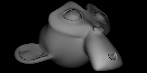
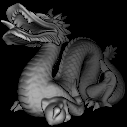
Figure 2: Synthetic test images. From left to right: Sombrero, Suzanne, Stanford Bunny and Dragon.

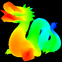
Figure 3: First column, from top to bottom: Input image, reprojected image, ground truth depth, computed depth for the Sombrero test image ($\alpha=7.5\times 10^{-5}$, $\tau=10^{-2}$, $n=10^{6}$). Second column: Ditto for the Stanford Bunny test image ($\alpha=7.5\times 10^{-5}$, $\tau=10^{-3}$, $n=10^{6}$). Third column: Ditto for the Dragon test image ($\alpha=7.5\times 10^{-8}$, $\tau=10^{-3}$, $n=10^{6}$).

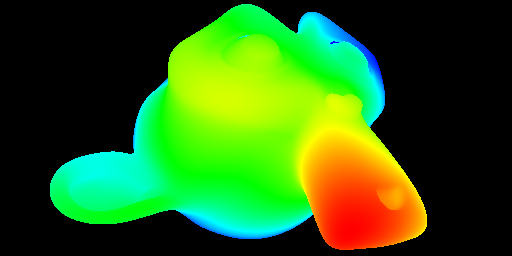
Figure 4: First row, from left to right: Input image and ground truth depth of the Suzanne test image. Second row: Reprojected image and the computed depth ($\alpha=10^{-7}$, $\tau=10^{-3}$, $n=10^{6}$).

Figure 5: Surface error maps. From left to right: Stanford Bunny, Dragon and Suzanne. Red denotes errors above 1 percent, where the intensity encodes the error magnitude. White denotes errors below 1 percent. The Sombrero is not shown, since the error is below 1 percent everywhere.

Results on Synthetic Test Images. In our first experiment we evaluate the reconstruction quality of our novel approach. To this end, we applied our perspective SfS algorithm to all four of the previously discussed test images and compared the reprojected image and the reconstruction to the ground truth; see Fig. 3 and Fig. 4. Herein, the depth values are colour-coded in such a way that depth increases from red via green to blue. As one can see, both the reprojected image as well as the estimated depth values coincide very well with the ground truth. This is also confirmed by the corresponding surface error maps in Fig. 5. Indeed, only small differences for the Stanford bunny (right paw) and the Dragon (tail tip) are visible. As a consequence both error measures which are listed in Table 2 are very small. Moreover, one can see that the proposed subquadratic penaliser outperforms a quadratic smoothness term in most cases. Only for the Sombrero which has a rather smooth surface, the reconstruction error is smaller in the quadratic case.

Table 2: Results for our approach with quadratic and subquadratic penaliser. Error measures are given in terms of the relative surface error (RSE) and the relative image error (RIE). Best results for each test image are highlighted boldface. Same parameters as in Fig. 3 and Fig. 4.

	quadratic						subquadratic
	RSE			RIE			RSE			RIE			runtime
Sombrero			0.00208			$0.00694$			$0.00318$			0.00209			$29113$s
Stanford Bunny			$0.00546$			$0.00015$			0.00439			0.00007			$23969$s
Dragon			0.01376			0.00028			0.01376			0.00028			$25350$s
Suzanne			$0.00392$			$0.00011$			0.00251			0.00002			$48395$s

Influence of the Regularisation. In our second experiment we investigate the influence of the regularisation on the quality of the reconstruction and its reprojection. To this end, we consider the Sombrero test image and vary the regularisation parameter $\alpha$ while the other parameters are kept fixed ($\tau=0.001$, $n=10^{4}$). The outcome is visualised in Fig. 6. While the reprojection related error measure (RIE) increases for a moderate amount of regularisation but is overall very low, the surface related error measure (RSE) decreases by almost a factor three (from $4.4\times 10^{-2}$ to $1.7\times 10^{-2}$). This, however, is not surprising, since the computed surface typically exhibits some form of smoothness and thus benefits from a moderate amount of regularisation. Since the actual purpose of SfS is to find the correct surface, this shows that the regularisation may have an overall positive impact on the quality of the results.

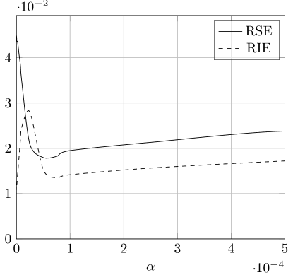
Figure 6: Impact of the amount of regularisation on the reconstruction quality and the reprojection accuracy for the Sombrero test image.

Independence of the Initialisation. In our third experiment we analyse the dependency of our approach on the initialisation. To this end, we use the Stanford Bunny ($z\in[1,2]$) and compare our initialisation on the coarsest scale of the proposed coarse-to-fine scheme (cf. Eq. (30)) with two other initialisations based on plain surfaces ($z=1$, $z=10$). The initial error and the outcome after $n=10^{6}$ iterations are listed in Table 3. While the initial error for a good guess ($z=1$) and a poor initialisation ($z=10$) differs significantly, the quality of the reconstruction and the reprojection is identical after sufficiently many iterations. This also holds for our initialisation which can be computed from the input image without requiring a specific knowledge of the depth. That all initialisations converge to the same solution, however, is not surprising since the estimation is embedded in our coarse-to-fine scheme.

Table 3: Impact of different initialisations on the reconstruction quality and reprojection accuracy for the Stanford Bunny ($\alpha=7.5\times 10^{-5}$, $\tau=10^{-3}$, $n=10^{6}$).

	initial error						after computation
	RSE			RIE			RSE			RIE
plane ($z=1$)			$0.25804$			$1.63174$			$0.00439$			$0.00007$
plane ($z=10$)			$6.41960$			$0.97373$			$0.00439$			$0.00007$
proposed			$0.37712$			$0.74363$			$0.00439$			$0.00007$

Comparison of Numerical Schemes. In our fourth experiment we compare the different numerical schemes proposed in Section 4: the full explicit scheme, the simplified explicit scheme and the alternating explicit scheme. In the first part of the experiment we juxtapose the quality of the different numerical schemes for equal stopping times (iterations $\times$ time step size). As one can see from the results in Table 4, the full explicit scheme clearly gives the best results in terms of reconstruction quality and reprojection accuracy. However, this comes at the expense of a significantly larger runtime, since more iterations are needed due to the time step restrictions discussed in Section 4. In fact the runtime is up to four orders of magnitude larger making the approach hardly feasible for larger image sizes. In the second part of the experiment we compared the numerical schemes for an equal number of iterations. From the results in Table 5 it becomes evident that in this case the simplified explicit scheme and in particular the alternating explicit scheme perform best in most cases in terms of reconstruction quality and reprojection accuracy. This demonstrates that it can be worthwhile to (partly) omit the terms that are added in the full explicit scheme since they slow down the convergence, but doing so does not necessarily compromise the quality.

Table 4: Comparison of different numerical schemes for equal stopping time $t=n\times\tau$. Results and runtimes refer to smaller versions of the four test images. Same parameters as in Fig. 3 and Fig. 4 except for $n$, which is given by $n=t/\tau$.

	alternating scheme						simplified scheme						full scheme
test image			RSE			RIE			RSE			RIE			RSE			RIE
Small Sombrero			$0.01823$			$0.01920$			$0.01820$			$0.02048$			0.00785			0.00527
($128\times 128$)			(runtime: $30$s)						(runtime: $15$s)						(runtime: $178021$s)
Small Stanford Bunny			$0.00659$			$0.00151$			$0.00667$			$0.00257$			0.00576			0.00097
($128\times 128$)			(runtime: $303$s)						(runtime: $150$s)						(runtime: $4278$s)
Small Dragon			$0.01667$			$0.00267$			$0.01673$			$0.00620$			0.01526			0.00205
($128\times 128$)			(runtime: $308$s)						(runtime: $149$s)						(runtime: $4304$s)
Small Suzanne			0.00899			$0.00514$			$0.01055$			$0.01909$			$0.01022$			0.00203
($128\times 96$)			(runtime: $223$s)						(runtime: $111$s)						(runtime: $2384$s)

Table 5: Comparison of different numerical schemes for equal number of iterations. Results refer to the smaller versions of the four test test images, see Tab. 4. The same parameters as in Fig. 3 and Fig. 4 have been used except for $n$, which is given by $n=10^{7}$.

	alternating scheme						simplified scheme						full scheme
test image			RSE			RIE			RSE			RIE			RSE			RIE
Small Sombrero			$0.02357$			0.00082			$0.02392$			$0.00659$			0.00358			$0.00319$
Small Stanford Bunny			$0.00390$			0.00001			0.00378			$0.00004$			$0.00489$			$0.00047$
Small Dragon			$0.00572$			0.00001			0.00562			0.00001			$0.00964$			$0.00170$
Small Suzanne			0.00319			$0.00002$			$0.00320$			0.00001			$0.00505$			$0.00056$

Table 6: Evaluation of inpainting properties for degraded versions of the Stanford Bunny test image. Same parameters as in Figure 7.

	perforated version			sliced version			original version
	(Fig. 7, top row)			(Fig. 7, bottom row)			(Fig. 2)
RSE			$0.00439$			$0.00509$			$0.00439$
RIE			$0.00039$			$0.00249$			$0.00007$

Reconstruction with Inpainting. In our fifth experiment we demonstrate the inpainting capabilities of the regularisation in combination with the confidence function $c$ embedded in the data term. For this reason we created a pair of degraded Stanford Bunny test images together with the corresponding confidence functions, which are both depicted in Fig. 7. In addition, the computed depth values and the reprojected images are shown. One can see that in both cases the missing regions in the input image can hardly deteriorate the quality of the results since the smoothness term fills in the information from the neighbourhood. This is also reflected in the error measures given in Table 6. In case of the perforated version the surface error even remains the same compared to the result for the original version.

Figure 7: First row, from left to right: Perforated version of the Stanford Bunny test image, corresponding confidence function $c$, computed depth values, reprojected image ($\alpha=7.5\times 10^{-5}$, $\tau=10^{-3}$, $n=10^{6}$). Second row: Ditto for the sliced version (same parameters).

Comparison with a PDE-Based Approach. In our seventh experiment we compare the results of our variational method with the PDE-based approach of Vogel et al. Vogel_SSVM2009 with Lambertian reflectance model. This essentially comes down to a comparison to the baseline method of Prados et al. Prados_CVPR2005 which is solved by Vogel et al. Vogel_SSVM2009 as part of a Phong-based model using an efficient fast marching scheme Sethian1999 . In this experiment we consider two scenarios, that nicely demonstrate the advantages and shortcomings of the different types of methods: On the one hand, we use input images without noise, on the other hand, we added Gaussian noise of standard deviation $\sigma=20$ before applying the two methods. The corresponding results are summarised in Tables 7 and 8, respectively. For the test images without noise both approaches give excellent results with errors among or below $1$ percent of the solution. Thereby the approach of Vogel et al. gives slightly better results in terms of the relative surface error (RSE), while the variational approach gives better results in terms of the relative image error (RIE). From the viewpoint of the variational approach this can be explained as follows: While the data term penalises deviations from the photometric reprojection error and thus gives rather small RIE values, the regulariser and the coarse-to-fine scheme yield a moderate smoothing of the surface resulting in slightly higher RSE values. In the case of the noisy input images the findings are completely different. Here, the variational method can take advantage of both the regulariser and the independence of the initialisation. While a higher smoothness weight allows to obtain a smooth surface, the hierarchical initialisation via the coarse-to-fine scheme does not require to rely on noisy solutions at critical points as the PDE-based approach of Vogel et al. As a consequence, the resulting surface errors of $3$ to $6$ percent for our variational approach are significantly lower than those of the PDE-based model ($11$ to $20$ percent). This can also be seen from the depth estimates for the Stanford Bunny depicted in Figure 8. Not surprisingly our findings are in full accordance with the observation in JBB2014 , in which the robustness of variational methods for perspective SfS has been investigated.

Table 7: Comparison between our variational method and the PDE-based approach of Vogel et al. Vogel_SSVM2009 with Lambertian reflectance model ($=$ baseline model of Prados et al. Prados_CVPR2005 ). Error measures are given in terms of the relative surface error (RSE) and the relative image error (RIE). Same parameters as in Fig. 3 and Fig. 4.

	Vogel et al. Vogel_SSVM2009						our method
	(PDE-based approach)						(variational method)
	RSE			RIE			RSE			RIE
Sombrero			$0.00301$			$0.00495$			$0.00318$			$0.00209$
Stanford Bunny			$0.00266$			$0.00154$			$0.00439$			$0.00007$
Dragon			$0.00422$			$0.00255$			$0.01376$			$0.00028$
Suzanne			$0.00253$			$0.00082$			$0.00251$			$0.00002$

Table 8: Performance under noise. Comparison between our variational method and the PDE-based approach of Vogel et al. Vogel_SSVM2009 with Lambertian reflectance model ($=$ baseline model of Prados et al. Prados_CVPR2005 ). Gaussian noise of standard deviation $\sigma=20$. Error measures are given in terms of the relative surface error (RSE) and the relative image error (RIE). The applied parameters are as follows: Sombrero ($\alpha=0.1$, $\tau=10^{-5}$, $n=10^{6}$), Stanford Bunny ($\alpha=1.0$, $\tau=10^{-5}$, $n=10^{6}$), Dragon ($\alpha=1.0$, $\tau=10^{-5}$, $n=10^{6}$), Suzanne ($\alpha=1.0$, $\tau=5\times 10^{-6}$, $n=10^{6}$).

	Vogel et al. Vogel_SSVM2009						Our method.
	(PDE-based approach)						(variational method)
	RSE			RIE			RSE			RIE
Noisy Sombrero			$0.19530$			$0.27254$			$0.05118$			$0.13239$
Noisy Stanford Bunny			$0.10973$			$0.17347$			$0.03235$			$0.15279$
Noisy Dragon			$0.12240$			$0.19409$			$0.05395$			$0.18767$
Noisy Suzanne			$0.12134$			$0.16783$			$0.01256$			$0.14302$

Figure 8: From left to right: Noisy version of the Stanford Bunny (Gaussian noise with $\sigma=20$), ground truth depth, computed depth using our variational approach ($\alpha=1.0$, $\tau=10^{-5}$, $n=10^{6}$), computed depth using the PDE-based approach of Vogel et al. Vogel_SSVM2009 with Lambertian model.

Results on Real-World Images. Finally, in order to evaluate our approach on real-world images, we used two images of faces provided by Prados PCF06 . According to Prados, these images have been taken with a cheap digital camera in a dark place, where the scene is illuminated by the flash of the camera. The focal length is $\mathtt{f}=5.8$mm and the grid size is approximately $h_{x}=h_{y}=0.018$mm. The test images as well as additional images rendered from a new viewpoint using the computed depth are shown in Fig. 9. In both cases the results look quite realistic. One can also see how the depth values at the eyes have been inpainted in the reconstruction, since a manually defined confidence function was used to mask out those regions where the assumption of a Lambertian surface is violated.

Figure 9: First row, from left to right: Face with closed eyes, three images rendered from a new viewpoint using the estimated depth ($\alpha=7.5\times 10^{-5}$, $\tau=5\times 10^{-3}$, $n=2\times 10^{5}$). Second row: Ditto for the second test image ($\alpha=7.5\times 10^{-5}$, $\tau=5\times 10^{-3}$, $n=2\times 10^{5}$).

7 Conclusion

In this paper, we described a novel variational model for perspective shape from shading that not only has many desirable theoretical properties but also yields very convincing reconstruction results for synthetic and real-world input images, even in the presence of noise or other deteriorations in an input image. While the arising optimisation problem has turned out to be challenging, we have proposed an alternating explicit scheme embedded in a coarse-to-fine framework that is robust with respect to the initialisation and that allows reasonable computation times compared to a standard explicit scheme.

Besides the results that are documented via extensive experiments in this chapter, let us point out that we see a main contribution of our work in a different context, as we have layed the fundamental building block for a conceptually correct, working variational framework that can combine perspective shape from shading with other techniques from computer vision such as e.g. stereo vision. We aim to explore the arising possibilities in a future work.

Acknowledgements. This work has been partially funded by the Deutsche Forschungsgemeinschaft (DFG) as a joint project (BR 2245/3-1, BR 4372/1-1).

8 Appendix

Alternative Derivation of the Surface Normal. Instead of computing the derivatives with respect to the 2-D image coordinates $x$ and $y$, one can also derive the surface normal in an alternative way that is often used in the literature, see e.g. Wu_IJCV2010 . The idea is to interpret the original surface in Eq. (4) as a function of the 3-D coordinates $X$, $Y$ and $Z(X,Y)$

$$\mathcal{S}\left(X(\mathbf{x},z),Y(\mathbf{x},z),Z(X(\mathbf{x},z),Y(\mathbf{x},z))\right)=\left[\begin{array}[]{c}X(\mathbf{x},z)\\ Y(\mathbf{x},z)\\ Z(X(\mathbf{x},z),Y(\mathbf{x},z))\end{array}\right]:=\left[\begin{array}[]{c}\dfrac{z\,x}{\mathtt{f}}\vspace{1ex}\\ \dfrac{z\,y}{\mathtt{f}}\vspace{1ex}\\ -z\end{array}\right]\,.$$ (52)

Dropping the dependency of $X$, $Y$ and $Z(X,Y)$ on $\mathbf{x}$, $z$ and computing the partial derivatives with respect to $X$ and $Y$ via the chain rule

$$\frac{\partial X}{\partial Y}=\frac{\partial X}{\partial x}\frac{\partial x}{\partial Y}\,,\qquad\qquad\qquad\frac{\partial Y}{\partial X}=\frac{\partial Y}{\partial y}\frac{\partial y}{\partial X}$$

then gives the tangent vectors to the surface

$$\mathcal{S}_{X}(\mathbf{x},z)=\left[\begin{array}[]{c}1\\[2.84526pt] \dfrac{z_{x}y}{z+z_{x}\,x}\\[8.53581pt] -\dfrac{z_{x}\,\mathtt{f}}{z+z_{x}\,x}\end{array}\right]\;,\;\;\;\;\;\mathcal{S}_{Y}(\mathbf{x},z)=\left[\begin{array}[]{c}\dfrac{z_{y}\,x}{z+z_{y}\,y}\\[11.38109pt] 1\\[2.84526pt] -\dfrac{z_{y}\,\mathtt{f}}{z+z_{y}\,y}\end{array}\right]\;.$$ (53)

After some computations we finally obtain the corresponding normal direction

$$\hat{\mathbf{n}}(\mathbf{x})=\mathcal{S}_{X}(\mathbf{x},z)\times\mathcal{S}_{Y}(\mathbf{x},z)=\dfrac{\mathtt{f}^{2}}{(z+z_{x}\,x)(z+z_{y}\,y)}\,\,\mathbf{n}(\mathbf{x})\,.$$ (54)

where $\mathbf{n}(\mathbf{x})$ is the normal direction from Eq. (8) As expected, both vectors only differ by scale, i.e. they have the same direction. Hence, the corresponding normalised vectors $\mathbf{n}/|\mathbf{n}|$ and $\hat{\mathbf{n}}/|\hat{\mathbf{n}}|$ are identical. While this alternative derivation was not used in our paper, it helps to clarify a common mistake in the literature that will be explained in the following.

Remark. Please note that, unlike in the orthographic case, the cross derivatives ${\partial X}/{\partial Y}$ and ${\partial Y}/{\partial X}$ do not vanish for the perspective model. Hence, using the orthographic derivation of the normal direction from Horn and Brooks HB89

$$\mathbf{n_{\mathrm{ortho}}}(\mathbf{x})=\frac{\partial}{\partial X}\!\left[\begin{array}[]{c}X\\ Y\\ Z\end{array}\right]\times\frac{\partial}{\partial Y}\!\left[\begin{array}[]{c}X\\ Y\\ Z\end{array}\right]=\left[\begin{array}[]{c}1\\ 0\\ Z_{X}\end{array}\right]\times\left[\begin{array}[]{c}0\\ 1\\ Z_{Y}\end{array}\right]=\left[\begin{array}[]{c}-Z_{X}\\ -Z_{Y}\\ 1\end{array}\right]$$ (55)

with zero cross derivatives and simply replacing the remaining partial derivatives $Z_{X}$ and $Z_{Y}$ by the corresponding expressions from (53) is not completely correct for the perspective case. Such an approach has for instance been proposed in Wu_IJCV2010 ; ZYT07 . It actually mixes the orthographic and the perspective model and thus typically gives worse results in the case of strong perspective distortions. Moreover, apart from not being completely correct, this strategy also yields significantly more complex models that typically require auxiliary variables to be solved, see again e.g. Wu_IJCV2010 ; ZYT07 .

References

- (1) Abdelrahim, A.S.: Three-Dimensional Modeling of the Human Jaw/Teeth Using Optics and Statistics. PhD thesis, Department of Electrical and Computer Engineering, University of Louisville, Louisville, Kentucky, USA (2014)
- (2) Abdelrahim, A.S., Abdelrahman, M.A., Abdelmunim, H., Farag, A., Miller, M.: Novel image-based 3D reconstruction of the human jaw using shape from shading and feature descriptors. In: Proc. British Machine Vision Conference, 1–11 (2011)
- (3) Abdelrahim, A.S., Abdelmunim, H., Graham, J., Farag, A.: Novel variational approach for the perspective shape from shading problem using calibrated images. In: Proc. IEEE International Conference on Image Processing, 2563–2566 (2013)
- (4) Ahmed, A., Farag, A.: A new formulation for shape from shading for non-Lambertian surfaces. In: Proc. IEEE Conference on Computer Vision and Pattern Recognition, 1817–1824 (2006)
- (5) Barles, G.: Solutions de viscosité des équations de Hamilton-Jacobi. Mathématiques Applications Vol. 17, Springer, 1994
- (6) Basha, T., Moses, Y. Kiryati, N.: Multi-view scene flow estimation: a view centered variational approach. International Journal of Computer Vision 101(1), 6–21 (2012)
- (7) Bors, A.G., Hancock, E.R., Wilson, R.C.: Terrain analysis using radar shape-from-shading. IEEE Transactions on Pattern Analysis and Machine Intelligence 25(8), 974–992 (2003)
- (8) Breuß, M., Cristiani, E., Durou, J.-D., Falcone, M., Vogel, O.: Numerical algorithms for perspective shape from shading. Kybernetika 46(2), 207–225 (2010)
- (9) Breuß, M., Cristiani, E., Durou, J.-D., Falcone, M. , Vogel, O.: Perspective shape from shading: ambiguity analysis and numerical approximations. SIAM Journal on Imaging Sciences 5(1), 311–342 (2012)
- (10) Brooks, M.J., Horn, B.K.P.: Shape and source from shading. In: Proc. International Joint Conference in Artificial Intelligence, 932–936 (1985)
- (11) Brox, T., Bruhn, A., Papenberg, N., Weickert, J.: High accuracy optical flow estimation based on a theory for warping. In: Proc. European Conference on Computer Vision, LNCS Vol. 3024, 25–36 (2004)
- (12) Camilli, F., Prados, E.: Viscosity solution. In Katsushi Ikeuchi (Ed.), The Encyclopedia of Computer Vision, Springer, 2014
- (13) Charbonnier, P., Blanc-Féraud, L., Aubert, G., Barlaud, M.: Deterministic edge-preserving regularization in computed imaging. IEEE Transactions on Image Processing 6(2), 298–311 (1997)
- (14) Crandall, M.G., Lions, P.-L.: Viscosity solutions of Hamilton-Jacobi equations. Transactions of the American Mathematical Society 277(1), 1–42 (1983)
- (15) Courant, R., Hilbert, D.: Methods of Mathematical Physics. Interscience Publishers, Inc., New York, NY (1953)
- (16) Courteille, F., Crouzil, A., Durou, J.-D., Gurdjos, P.: Towards shape from shading under realistic photographic conditions. In: Proc. IEEE International Conference on Pattern Recognition, 277–280 (2004)
- (17) Courteille, F., Crouzil, A., Durou, J.-D., Gurdjos, P.: 3D-spline reconstruction using shape from shading: spline from shading. Image and Vision Computing 26(4), 466–479 (2008)
- (18) Demetz, O., Stoll, M., Volz, S., Weickert, J., Bruhn, A.: Learning brightness transfer functions for the joint recovery of illumination changes and optical flow. In: Proc. European Conference on Computer Vision, LNCS Vol. 8689, 455–471 (2014)
- (19) Diggelen, J.V.: A photometric investigation of the slopes and heights of the ranges of hills in the maria of the moon. Bulletin of the Astronomical Institutes of the Netherlands XI(423), 283–289 (1951)
- (20) Durou, J.-D., Falcone, M., Sagona, M.: Numerical methods for shape-from-shading: a new survey with benchmarks. Computer Vision and Image Understanding 109(1), 22–43 (2008)
- (21) Estellers, V., Thiran, J.-P., Gabrani, M.: Surface reconstruction from microscopic images in optical lithography. IEEE Transactions on Image Processing 23(8), 3560–3573 (2014)
- (22) Frankot, R.T., Chellappa, R.: A method for enforcing integrability in shape from shading algorithms. IEEE Transactions on Pattern Analysis and Machine Intelligence 10(4), 439–451 (1988)
- (23) Hartley, R., Zisserman, A.: Multiple View Geometry in Computer Vision. Cambridge University Press (2004)
- (24) Horn, B.K.P.: Shape from Shading: A Method for Obtaining the Shape of a Smooth Opaque Object from One View. PhD thesis, Department of Electrical Engineering, MIT, Cambridge, Massachusetts, USA (1970)
- (25) Horn, B.K.P.: Robot Vision. MIT Press (1986)
- (26) Horn, B.K.P., Brooks, M.J.: The Variational Approach to Shape from Shading. Computer Vision, Graphics, and Image Processing 33, 174–208 (1986)
- (27) Horn, B.K.P., Brooks, M.J.: Shape from Shading. Artificial Intelligence Series, MIT Press (1989)
- (28) Ikeuchi, K., Horn, B.K.P.: Numerical shape from shading and occluding boundaries. Artificial Intelligence 17(1–3), 141–184 (1981)
- (29) Ju, Y. C., Breuß, M., Bruhn, A.: Variational perspective shape from shading. In: Proc. International Conference on Scale Space and Variational Methods in Computer Vision, LNCS Vol. 9087, 538–550 (2015).
- (30) Kimmel, R., Siddiqi, K, Kimia, B.B., Bruckstein, A.M.: Shape from shading: level set propagation and viscosity solutions. International Journal of Computer Vision 16, 107–133 (1995)
- (31) Lysaker, M., Lundervold, A., Tai, X.-C.: Noise removal using fourth-order partial differential equation with applications to medical magnetic resonance images in space and time. IEEE Transactions on Image Processing 12(12), 1057–1590 (2003)
- (32) Mecca, R., Falcone, M.: Uniqueness and approximation of a photometric shape-from-shading model. SIAM Journal on Imaging Science 6, 616–659 (2013)
- (33) Mecca, R., Wetzler, A., Bruckstein, A.M., Kimmel, R.: Near Field Photometric Stereo with Point Light Sources. SIAM Journal on Imaging Sciences 7(4), 2732–2770 (2014)
- (34) Okatani, T., Deguchi, K.: Shape reconstruction from an endoscope image by shape from shading technique for a point light source at the projection center. Computer Vision and Image Understanding 66 (1997) 119–131
- (35) Oliensis, J.: Shape from shading as a partially well-constrained problem. Computer Vision, Graphics, and Image Processing: Image Understanding 54(2), 163–183 (1991)
- (36) Oren, M., Nayar, S.; Generalization of the Lambertian model and implications for machine vision. International Journal of Computer Vision 14(3), 227–251 (1995)
- (37) Phong, B.T.: Illumination for computer-generated pictures. Communications of the ACM 18(6), 311–317 (1975)
- (38) Prados, E., Faugeras, O.: “Perspective shape from shading” and viscosity solutions. In: Proc. IEEE International Conference Computer Vision, 826–831 (2003)
- (39) Prados, E., Faugeras, O.: Shape from shading: a well-posed problem? In: Proc. IEEE Conference on Computer Vision and Pattern Recognition, 870–877 (2005)
- (40) Prados, E., Camilli, F., Faugeras, O.: A unifying and rigorous shape from shading method adapted to realistic data and applications. Journal of Mathematical Imaging and Vision 25(3), 307–328 (2006)
- (41) Rindfleisch, T.: Photometric method for lunar topography. Photogrammetric Engineering 32(2), 262–277 (1966)
- (42) Robert, L., Deriche, R.: Dense depth map reconstruction: a minimization and regularization approach which preserves discontinuities. In: Proc. European Conference on Computer Vision, LNCS Vol. 1064, 439–451 (1996)
- (43) Rouy, E. , Tourin, A.: A viscosity solution approach to shape-from-shading. SIAM Journal on Numerical Analysis 29(3), 867–884 (1992)
- (44) Schmaltz, C., Peter, P., Mainberger, M., Eberl, F., Weickert, J., Bruhn, A.: Understanding, optimising, and extending data compression with anisotropic diffusion. International Journal of Computer Vision 108(3), 222–240 (2014)
- (45) Sethian, J.: Level Set Methods and Fast Marching Methods. Cambridge University Press (1999)
- (46) Tankus, A., Sochen, N, Yeshurun, Y.: A new perspective [on] shape-from-shading. In: Proc. IEEE International Conference on Computer Vision, 862–869 (2003)
- (47) Tankus, A., Sochen, N, Yeshurun, Y.: Shape-from-shading under perspective projection. International Journal of Computer Vision 63(1), 21–43 (2005)
- (48) Vogel, O., Breuß, M., Weickert, J.: Perspective shape from shading with non-Lambertian reflectance. In: Proc. German Conference on Pattern Recognition, LNCS Vol. 5096, 517–526 (2008)
- (49) Vogel, O., Bruhn, A., Weickert, J., Didas, S.: Direct shape-from-shading with adaptive higher order regularisation. In: Proc. International Conference on Scale Space and Variational Methods in Computer Vision, LNCS Vol. 4485, 871–882 (2007)
- (50) Vogel, O., Breuß, M., Leichtweis, T., Weickert, J.: Fast shape from shading for Phong-type surfaces. In: Proc. International Conference on Scale Space and Variational Methods in Computer Vision, LNCS Vol. 5567, 733–744 (2009)
- (51) Wang, G.H., Han, J.Q., Zhang, X.M.: Three-dimensional reconstruction of endoscope images by a fast shape from shading method. Measurement Science and Technology 20(12), (2009)
- (52) Wu, C., Narasimhan, S., Jaramaz, B.: A multi-image shape-from-shading framework for near-lighting perspective endoscopes. International Journal of Computer Vision 86, 211–228 (2010)
- (53) Yuen, S.Y., Tsui, Y.Y., Chow, C.K.: A fast marching formulation of perspective shape from shading under frontal illumination. Pattern Recognition Letters 28(7), 806–824 (2007)
- (54) Zhang, R., Tsai, P.-S., Cryer, J.E., Shah, M.: Shape from shading: a Survey. IEEE Transactions on Pattern Analysis and Machine Intelligence 21(8), 690–706 (1999)
- (55) Zhang, L., Yip, A. M., Tan, C. T.: Shape from shading based on Lax-Friedrichs fast sweeping and regularization techniques with applications to document image restoration. In: Proc. IEEE Conference on Computer Vision and Pattern Recognition, 1–8 (2007)
- (56) Zhang, L., Yip, A. M., Tan, C. T.: A restoration framework for correcting photometric and geometric distortions in camera-based document images. In: Proc. IEEE International Conference on Computer Vision, 1–8 (2007)
- (57) http://www.blender.org (Last visited on 05/05/2015).
- (58) The Stanford 3D Scanning Repository, http://graphics.stanford.edu/data/3Dscanrep/ (Last visited on 05/05/2015).