Condensate formation in a zero-range process with random site capacities

Abstract

We study the effect of quenched disorder on the zero-range process (ZRP), a system of interacting particles undergoing biased hopping on a one-dimensional periodic lattice, with the disorder entering through random capacities of sites. In the usual ZRP, sites can accommodate an arbitrary number of particles, and for a class of hopping rates and high enough density, the steady state exhibits a condensate which holds a finite fraction of the total number of particles. The sites of the disordered zero-range process considered here have finite capacities chosen randomly from the Pareto distribution. From the exact steady state measure of the model, we identify the conditions for condensate formation, in terms of parameters that involve both interactions (through the hop rates) and randomness (through the distribution of the site capacities). Our predictions are supported by results obtained from a direct numerical sampling of the steady state and from Monte Carlo simulations. Our study reveals that for a given realization of disorder, the condensate can relocate on the subset of sites with largest capacities. We also study sample-to-sample variation of the critical density required to observe condensation, and show that the corresponding distribution obeys scaling, and has a Gaussian or a Lévy-stable form depending on the values of the relevant parameters.

Keywords: Zero-range processes, Disordered systems (theory), Stationary states

1 Introduction and model

Quenched disorder can strongly affect both static and time-dependent properties of statistical systems. Of particular interest is the case of driven systems in which a dynamics that violates detailed balance leads the system to a nonequilibrium stationary state (NESS) that cannot be described within the purview of the Boltzmann-Gibbs equilibrium statistical mechanics. In this work, we explore effects of quenched disorder by analyzing a one-dimensional model of a disordered nonequilibrium system, namely, a disordered zero-range process. The model is a modification of the well-studied zero-range process (ZRP), a lattice model of interacting particles evolving in presence of an external drive, with no limit on the capacity of each site to hold any number of particles [1, 2, 3, 4]. Here, we study a disordered model introduced in [5, 6], in which the capacity of each site is a randomly chosen finite number. Knowledge of the exact steady state of this model allows us to unveil and understand the physical effects that result from quenched disorder. We are primarily interested in the possible occurrence of a condensate, which is a quintessential feature of the ZRP, as discussed below.

On a one-dimensional periodic lattice, the ZRP dynamics involves particles undergoing stochastic hopping between the lattice sites [1, 2, 3, 4]. For a system of $L$ sites and $N$ indistinguishable unit-mass particles, a unit time step of the dynamics comprises $L$ sequential moves, in each of which a particle hops out of a random site $i;\leavevmode\nobreak\ i=1,2,\ldots,L$, with occupancy $n_{i};\leavevmode\nobreak\ n_{i}>0$, with a specified hop rate $u_{i}(n_{i})$, and moves to site $i+1$. The particle density is $\rho\equiv N/L$. The forward-biased hopping of a particle from a site to only its right neighbor incorporates the effect of an external driving field on the particles. Evidently, the dynamics conserves the total number of particles in the system. While there is no interaction between particles on different sites, that between particles on the same site may be modeled through the dependence of the hop rate of a particle from the site on its occupancy. Remarkably, the NESS measure of configurations in the ZRP can be found exactly for any choice of hop rates and in any spatial dimension [1, 2, 3, 4]. The homogeneous ZRP is defined by having the same functional form of the hop rate for all sites.

The phenomenon of real-space condensation that can occur in the steady state of the ZRP involves a finite fraction of particles accumulating on a single site, thereby forming a macroscopic condensate whose mass increases with increasing density. In the case of the homogeneous ZRP, a possible choice of the hop rate is $u(n)=1+b/n$, where $b>0$ is a finite constant. Such a form of the hop rate implies an effective attraction between particles on the same site. For such a choice, it is known that for $b>2$, the model in the NESS exhibits a transition to a condensate phase at a critical value of the particle density given by $\rho_{c}=1/(b-2)$ [3]. For densities $\rho<\rho_{c}$, the system is in a fluid phase characterized by an occupancy of order unity on every site and a single-site occupancy distribution $p(n)$ that decays exponentially for large $n$. At the transition point $\rho=\rho_{c}$, the distribution decays asymptotically as a power-law, corresponding to a critical fluid. Above $\rho_{c}$, the critical fluid coexists with a macroscopic aggregate (the “condensate”), so that in addition to a power-law part, the distribution $p(n)$ has a sharp peak around $n=(\rho-\rho_{c})L$ that represents the condensate. The ZRP has been invoked to model condensation in a number of contexts, e.g., clustering of particles in shaken granular systems [7], jams in traffic flows [8], wealth condensation in macroeconomies [9], and other systems.

Driven diffusive systems constitute a class of stochastically evolving interacting particle systems typified by a spreading of density fluctuations with a systematic drift in addition to a diffusive motion [10, 11, 12]. At long times, these systems relax to a NESS in which a steady current of particles flows through the system. The forward-biased ZRP described above is an example of a driven diffusive system, and can also be mapped to another paradigmatic and extensively studied model in this class, namely, the asymmetric simple exclusion process (ASEP). On a one-dimensional periodic lattice, the ASEP involves indistinguishable hard-core particles undergoing biased hopping to empty nearest-neighbor sites. The mapping between the ZRP and the ASEP consists in interpreting sites (respectively, particles) in the former as particles (respectively, empty sites) in the latter [3].

Quenched disorder in driven diffusive systems has been studied over the years in several types of systems in this class [13]. Both particle-wise disorder, in which different particles have different time-independent hop rates [14, 15, 16, 17, 18], and space-wise disorder, with time-independent hop rates that are randomly distributed in space [5, 6, 19, 20, 21, 22, 23, 24], have been considered. Note that the mapping between the ASEP and the ZRP mentioned above transforms particle-wise disorder in the ASEP into space-wise disorder in the corresponding ZRP [14, 15]. Other studies of quenched disorder in driven systems include a disordered ASEP with particle non-conservation, in which randomly chosen sites do not conserve particle number [25], a ZRP on inhomogeneous networks, in which particles hop between nodes of a network with one node of degree much higher than a typical degree [26], a ZRP with quenched disorder in the particle interaction, implemented through a small perturbation of a generic class of hop rates [27, 28], and a ZRP involving an interplay between on-site interaction and diffusion disorder [29].

In contrast to the above mentioned studies of quenched disorder, in the model under consideration here, disorder is assigned to the capacities of sites; the capacity is a random variable that restricts the number of particles a site can accommodate. This model was introduced in [5, 6] as the disordered drop-push process (DDPP) to study transport of carriers trapped in local regions of space, and is a generalization of the uniform drop-push process [30, 31]. As pointed out in [2], the drop-push process is actually a special case of the ZRP, with infinite hopping rates out of sites in which the occupancy exceeds the capacity. We thus prefer to refer to the model as the random capacity zero-range process (RC-ZRP). The fact that capacities are finite and random has a strong and an essential influence on the ZRP steady-state dynamics, as we discuss below.

In this paper, we consider capacities chosen independently for every site from a common distribution with power-law tails. For a one-dimensional periodic lattice with $L$ sites, every site $i$ has a capacity $l_{i}$ chosen independently from the Pareto distribution:

$$P(l)=\frac{\alpha}{l^{1+\alpha}};\leavevmode\nobreak\ \leavevmode\nobreak\ \alpha>0,\leavevmode\nobreak\ {\rm and\leavevmode\nobreak\ }l\in[1,\infty).$$ (1)

Note that for a given realization $\{l_{i}\}$ of the disorder, the system can accommodate at most $N_{\rm max}\equiv\sum\limits_{i=1}^{L}l_{i}$ particles .

A new feature, namely, a dynamical cascade effect, emerges owing to sites having restricted capacities in the RC-ZRP [5, 6, 30, 31]. Consider a particle hopping out of a random site $i$ that has occupancy $0<n_{i}\leq l_{i}$ with hop rate $u_{i}(n_{i}|l_{i})$, and moving to site $i+1$. If the site $i+1$ is already full, a particle from this site gets pushed further right, and so on, leading to a sequence of adjacent-site hops that continues until a particle hops into a site ($i+m$, say) that was not fully occupied earlier (i.e., $n_{i+m}<l_{i+m}$). Note that a unit time step corresponds to $L$ updates at randomly chosen sites, where each update may involve several particle hops out of fully filled sites. Thus, restricted capacities lead to a cascade of particle transfers through filled sites, explaining the nomenclature “drop-push process” used in [30, 31]. Figure 1 shows a schematic view of the RC-ZRP.

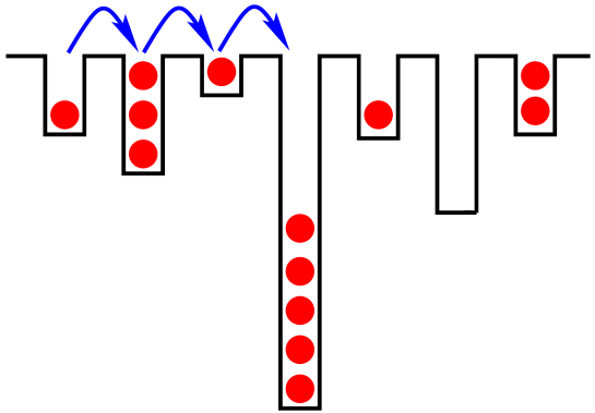
Figure 1: Schematic diagram of the random capacity zero-range process, showing a typical configuration and possible particle hops.

In this paper, we ask: Does restricting the ZRP site capacity, as in the RC-ZRP, still allow for the formation of a condensate, and if so, under what conditions? Let us consider a form for the hop rate $u_{i}(n|l_{i})$ that promotes condensate formation in the homogeneous ZRP, namely, $u_{i}(n>0)=1+b/n\leavevmode\nobreak\ \forall\leavevmode\nobreak\ i$, with $b>0$. The hop rate is taken to have this form for occupancies in the range $0<n\leq l_{i}$, and to be infinite for occupancies larger than $l_{i}$ [2], ensuring an immediate movement of a particle from a filled site to one that is not full:

$$u_{i}(n|l_{i})=\left\{\begin{array}[]{cc}0&\mbox{for\leavevmode\nobreak\ }n=0,\\ 1+\frac{b}{n}&\mbox{for\leavevmode\nobreak\ }0<n\leq l_{i},\\ \infty&\mbox{for\leavevmode\nobreak\ }n>l_{i}.\end{array}\right.$$ (2)

Note that in contrast to earlier studies of the model in [5, 6] which considered general hop rates, the choice (2) has the possibility of supporting condensate formation. In this paper, we demonstrate on the basis of exact analytical and simulation results that an interplay of the capacity distribution (1) with the hop rate (2) can indeed lead to condensate formation, and derive the conditions for this to happen. It should be noted that the steady state equal-time properties reported in this paper hold not just for the considered case of biased hopping of particles from a site to its right neighbor, but also for unbiased hopping to the left and to the right neighboring site. This is because, as we discuss in Section 2, the steady state measure of the RC-ZRP is the same in the two cases. However, unequal-time properties in the steady state, for instance, relocation dynamics of the condensate, will be different for biased and unbiased hopping.

The ZRP in which sites have bounded capacities was addressed recently in [32]. Unlike our model, the capacity was taken to be the same for all sites, and quenched disorder was introduced through site-dependent and particle-dependent hop-rates, leading to dynamical blocking that causes slow relaxation to steady state.

The layout of the paper is as follows. In Section 2, we discuss the steady state of the RC-ZRP, based on which we derive in Section 3 the conditions to obtain condensation in the model. In Section 4, we confirm our predictions by a direct numerical sampling of the steady state and by performing Monte Carlo simulations of the steady-state dynamics. We also discuss the relocation dynamics of the condensate. The paper ends with conclusions in Section 5, while the Appendix summarizes some relevant features associated with the capacity distribution.

2 Stationary state

The RC-ZRP relaxes at long times to a current-carrying nonequilibrium stationary state. Using the condition of pairwise balance [30], as in [5, 6], the steady state measure of configurations may be found. For a given realization $\{l_{i}\}$ of the disorder and a given total number of particles $N\leq N_{\rm max}$, it has a factorized form :

$${\cal P}(\{n_{i}\}|\{l_{i}\},N)\propto\prod\limits_{i=1}^{L}f_{i}(n_{i}|l_{i})\delta\left(\sum\limits_{i=1}^{L}n_{i},N\right),$$ (3)

where $\delta(m,n)$ is the Kronecker Delta function, while the single-site factors $f_{i}(n|l_{i})$ equal unity for $n=0$ and are given for $n>0$ by

$$f_{i}(n|l_{i}) \equiv \left[\prod\limits_{m=1}^{n}u_{i}(m|l_{i})\right]^{-1}$$ (4)

$$= \left\{\begin{array}[]{cc}\frac{\Gamma(b+n+1)}{\Gamma(n+1)\Gamma(b+1)}&\mbox{for\leavevmode\nobreak\ }0<n\leq l_{i},\\ 0&\mbox{for\leavevmode\nobreak\ }n>l_{i},\end{array}\right.$$ (7)

where $\Gamma(x)$ is the Gamma function. Here, in arriving at the second equation, we have used Eq. (2).

Equation (3) is the measure of configurations within the canonical ensemble. In the thermodynamic limit $N\to\infty,L\to\infty$, keeping the overall particle density $\rho\equiv N/L$ fixed, we use an equivalent grand canonical ensemble description of the steady state. In such a description, the total number of particles is allowed to fluctuate, and a fugacity $z$ fixes the average number of particles to equal $N$. The steady state measure of configurations within the grand canonical ensemble is given by

$${\rm Prob}(\{n_{i}\}|\{l_{i}\})\propto\prod_{i=1}^{L}p_{i}(n_{i}|l_{i}),$$ (8)

where $p_{i}(n|l_{i})$ is the single-site occupancy distribution, namely, the probability for the $i$th site to have $0\leq n\leq l_{i}$ particles:

$$p_{i}(n|l_{i})\equiv\frac{z^{n}f_{i}(n|l_{i})}{F_{i}(z|l_{i})},$$ (9)

with $F_{i}(z|l_{i})$ ensuring normalization of $p_{i}(n|l_{i})$:

$$F_{i}(z|l_{i})\equiv 1+\sum_{n=1}^{l_{i}}z^{n}f_{i}(n|l_{i}).$$ (10)

Here, the fugacity $z$ satisfies $\sum_{i=1}^{L}\overline{n_{i}}=N$, where $\overline{n_{i}}=d\ln F_{i}(z|l_{i})/d\ln z$ is the average occupancy at the $i$th site, with the average taken with respect to the single-site probability (9). We finally get

$$\frac{1}{L}\sum_{i=1}^{L}\frac{zF_{i}^{\prime}(z|l_{i})}{F_{i}(z|l_{i})}=\rho,$$ (11)

where prime denotes differentiation with respect to $z$.

As discussed in the Appendix, the maximum number of particles $N_{\rm max}$ that can be accommodated in the system scales with $L$ as $N_{\rm max}\sim L^{1/\alpha}$ for $\alpha<1$, and as $N_{\rm max}=aL$ for $\alpha>1$, where $a\equiv\int dl\leavevmode\nobreak\ lP(l)$ is finite. It then follows that in the latter case, the density $\rho$ in Eq. (11) has a maximum allowed finite value equal to $a$, while for $\alpha<1$, $\rho$ diverging with $L$ as $L^{1/\alpha-1}$ can be arbitrarily large. For a given value of $z$, evaluating numerically the left hand side of Eq. (11) for a given realization of disorder, and then averaging with respect to disorder, we show in Fig. 2 the disorder-averaged $\rho$, denoted by $\langle\rho\rangle$, as a function of $z$ for three different system sizes .

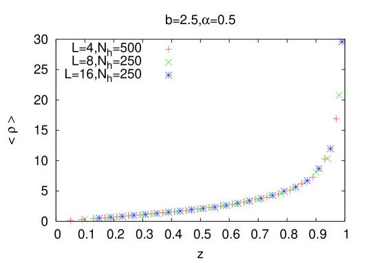
Figure 2: Disorder-averaged density $\langle\rho\rangle$ versus fugacity $z$, computed using Eq. (11) for $b=2.5$ and $\alpha=0.5$. The system sizes are marked in the figure. Here, $N_{h}$ is the number of disorder realizations over which the data have been averaged.

The occupancy distribution for the full system is defined as the probability that a randomly chosen site has $n$ particles. This is possible only if the site capacity is equal to or larger than $n$, so that the distribution has the form

$$\widetilde{p}(n)\propto z^{n}f(n)\int_{n}^{\infty}dl\leavevmode\nobreak\ P(l).$$ (12)

For large $n\gg 1$, Eq. (7) combined with the approximation $\Gamma(b+n+1)/\Gamma(n+1)\approx n^{b}+O(n^{b-1})$ yields the following asymptotic behavior:

$$p_{i}(n|l_{i})\propto\frac{\exp(-n/n^{\star})}{n^{b}},$$ (13)

$$\widetilde{p}(n)\propto\frac{\exp(-n/n^{\star})}{n^{b+\alpha}},$$ (14)

where the characteristic occupancy $n^{\star}$ is given by

$$n^{\star}\equiv-1/\ln(z).$$ (15)

The RC-ZRP in the NESS supports a steady current of particles through the system. Within the grand canonical ensemble, an exact expression for the average steady-state current for a given realization of disorder was derived in [6]. We briefly summarize the derivation here. From the dynamics, it is evident that all hops contributing to the current $J_{i-1,i}$ across the bond $(i-1,i)$ for which site $i$ is completely full also contribute to $J_{i,i+1}$, so that one has the recursion

$$J_{i,i+1}=p_{i}(l_{i}|l_{i})J_{i-1,i}+\sum_{n_{i}=1}^{l_{i}}u_{i}(n_{i}|l_{i})p_{i}(n_{i}|l_{i}),$$ (16)

where the second term on the right hand side is due to hops originating from site $i$. Now, steady state implies that all the bond currents are equal, $J_{i,i+1}=J_{i-1,i}=\ldots=J_{0}$, so that the above equation yields

$$J_{0}={{\sum_{n_{i}=1}^{l_{i}}u_{i}(n_{i}|l_{i})p_{i}(n_{i}|l_{i})}\over{1-p_{i}(l_{i}|l_{i})}}=z,$$ (17)

where we have used Eqs. (4) and (9). The steady-state current depends through the fugacity $z$ on the overall particle density $\rho$ and the number of sites of different capacities in a given realization of disorder (see Eq. (11)), thus becoming a function of $b$ and $\alpha$. Note that the expression (17) for the average steady-state current in terms of the fugacity $z$ is the same as for the usual ZRP [3].

In the following section, we address the issue of condensate formation in the RC-ZRP.

3 Condensate formation

In this section, we turn to the conditions for condensate formation in the RC-ZRP. We also study the distribution of the critical density $\rho_{c}$ to observe condensation, and its scaling as a function of $L$. We begin by summarizing the main questions and the results before getting to the details of the derivation.

It is useful to first recall the known scenario of condensation in the customary homogeneous ZRP [3]. Since there is no restriction on site capacities, there is no difficulty in accommodating $O(L)$ particles on any one site. An essential requirement for condensation is the existence of a finite critical value of the average site occupancy in the limit the fugacity $z$ attains its maximum possible value $z_{\rm max}$. Below this critical value of the density, all sites have the same average occupancy equal to the overall density of particles in the system. Above the critical value, the average occupancy of all but one site has the critical value; the excess particles that form a finite fraction of the total number of particles are accommodated on a single randomly-chosen site.

In this backdrop, it is a priori not apparent whether and when such a scenario of condensation holds in the RC-ZRP in which sites have restricted capacities. To address the issue, we argue as follows.

1. A necessary condition for condensate formation is that at least one site be able to accommodate $O(L)$ particles. In view of sites having restricted capacities in the RC-ZRP, the candidate for a site that can accommodate a macroscopic number of particles is the one with the largest capacity. Then, if the largest capacity $l_{\rm max}\equiv{\rm Max}[l_{1},l_{2},\ldots,l_{L}]$ has the scaling $l_{\rm max}\sim L^{\theta}$, we need $\theta$ to be larger than unity for condensate formation.

2. Additionally, we require that the average site occupancy has a finite value, denoted by $\rho_{c}$, as $z\to z_{\rm max}$.

3. When conditions (i) and (ii) are fulfilled, condensate formation is possible at high enough density $\rho>\rho_{c}$. The critical density $\rho_{c}$ depends on the realization of disorder, and the question arises as to how the form of the disorder-induced distribution ${\rm Prob}(\rho_{c})$ of $\rho_{c}$ depends on the relevant parameters.

Whether conditions (i) and (ii) above would hold depends on parameters that characterize the probability distribution of capacities (Eq. (1)) and the form of the hop rate (Eq. (2)), namely, the exponents $\alpha$ and $b$. The results are as follows:

1. The exponent $\theta$ is given by $1/\alpha$, so the site with the largest capacity can accommodate $O(L)$ particles provided that $\alpha<1$.

2. The average site occupancy remains finite as $z\to z_{\rm max}$ so long as one has $b+\alpha>2$.

   Combining the last two points, we thus arrive at the following conditions for condensate formation in the RC-ZRP:

   $$b+\alpha>2,\leavevmode\nobreak\ \leavevmode\nobreak\ \leavevmode\nobreak\ \leavevmode\nobreak\ {\rm\leavevmode\nobreak\ and\leavevmode\nobreak\ }\alpha<1\leavevmode\nobreak\ \leavevmode\nobreak\ \leavevmode\nobreak\ \leavevmode\nobreak\ \leavevmode\nobreak\ ({\rm Conditions\leavevmode\nobreak\ to\leavevmode\nobreak\ obtain\leavevmode\nobreak\ condensation}).$$ (18)

3. The distribution ${\rm Prob}(\rho_{c})$ is a Gaussian for $b>(4-\alpha)/2$, while it is a Lévy-stable distribution for $1<b<(4-\alpha)/2$.

These results are summarized in Fig. 3, which shows the regime for condensate formation in the $\alpha-b$ plane, and also the forms of ${\rm Prob}(\rho_{c})$ in different regions.

The issue of sample-dependence of phase transitions was studied numerically in [24] for the one-dimensional ASEP with open boundaries and quenched-disordered hopping rates. In the present work, we are able to determine the analytic forms for the distribution of the critical density because of the product form of the steady state measure in the RC-ZRP with periodic boundary conditions.

In the limit $\alpha\to 0$, the capacities become infinitely large, and the RC-ZRP dynamics becomes similar to the dynamics of the homogeneous ZRP. In this limit, the condition to observe condensation becomes the requirement $b>2$, a result known for the homogeneous ZRP [3].

We now proceed to a derivation and a more detailed discussion of our results.

Figure 3: In the $\alpha-b$ plane, the dashed regions are those for which the system exhibits a condensate; the corresponding forms of the $\rho_{c}$ distribution are also indicated.

3.1 The largest capacity $l_{\rm max}$

In order to accommodate the condensate, it is necessary that $l_{\rm max}$ grows sufficiently rapidly with $L$, namely, as $L^{\theta}$, with $\theta>1$. For the Pareto distribution of Eq. (1), it is known that $l_{\rm max}$ scales as $L^{1/\alpha}$, see the Appendix. Thus, condensate formation is possible provided that $\alpha\leq 1$.

As discussed in the Appendix, not just the site with capacity $l_{\rm max}$, but in fact several sites have capacities of order $L^{1/\alpha}$. This feature allows the condensate to form and relocate in time on other sites that belong to this subset. The numerical studies reported in Section 4 bear this out.

3.2 Average site occupancy

Let us now investigate the behavior of the average site occupancy as $z\to z_{\rm max}$, in the regime $\alpha<1$ as required to accommodate a putative condensate (Section 3.1). The quantity $z_{\rm max}$ is obtained by requiring the convergence of the series $F_{i_{1}}(z)\equiv 1+\sum\limits_{n=1}^{l_{\rm max}}z^{n}f_{i_{1}}(n)$ in the limit $L\to\infty$, where $i_{1}$ is the label for the site with the largest capacity. We obtain $z_{\rm max}=1$ as the radius of convergence of the series. The average site occupancy being a monotonically increasing function of $z$ has a maximum allowed value in the limit $z\to z_{\rm max}$, given by

$$\rho^{\star}(\{l_{i}\}) \equiv \lim_{z\to z_{\rm max}}\frac{1}{L}\sum_{i=1}^{L}\frac{zF_{i}^{\prime}(z|l_{i})}{F_{i}(z|l_{i})}$$ (19)

$$= \frac{1}{L}\sum\limits_{i=1}^{L}G(l_{i});\leavevmode\nobreak\ \leavevmode\nobreak\ \leavevmode\nobreak\ \leavevmode\nobreak\ G(l_{i})\equiv\frac{\sum_{n=1}^{l_{i}}nf_{i}(n|l_{i})}{1+\sum_{n=1}^{l_{i}}f_{i}(n|l_{i})},$$

which defines a characteristic density $\rho^{\star}$ for every disorder realization. Evidently, the density $\rho^{\star}(\{l_{i}\})$ is given by a sum of $L$ i.i.d. random variables $G(l_{i});\leavevmode\nobreak\ i=1,2,\ldots,L$. A finite value of $\rho^{\star}$ implies condensate formation for $\rho>\rho^{\star}$, so that $\rho^{\star}$ coincides with the critical density $\rho_{c}$ to obtain condensation. From Eq. (19), we get the corresponding disorder-averaged characteristic density as

$$\langle\rho^{\star}\rangle\equiv\int_{1}^{\infty}dl\leavevmode\nobreak\ P(l)G(l).$$ (20)

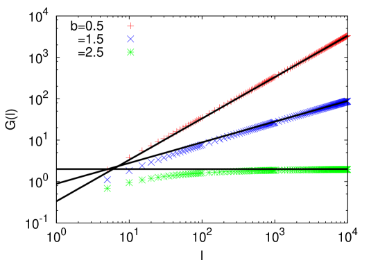
Figure 4: $G(l)$ as a function of $l$ for three representative values of $b$, obtained by evaluating numerically Eq. (21). The black lines stand for the asymptotic behavior, Eq. (22).

The behavior of $\rho^{\star}$ is governed by two parameters, namely, the exponent $\alpha$ that characterizes the probability distribution of the capacities, and the exponent $b$ that characterizes the hop rate. Let us ask for the condition on the allowed range of values of $b$ and $\alpha$ that leads to a finite $\langle\rho^{\star}\rangle$. Using Eq. (7), the function $G(l)$ in Eq. (19) can be expressed as

$$G(l)=\frac{1}{b-2}+\frac{(b-1)(l+1)}{(b-2)\Big{(}1-\Gamma(b+l+1)/[\Gamma(b)\Gamma(l+2)]\Big{)}},$$ (21)

implying that $G(l)$ diverges for particular values $b=1,2$. In the asymptotic regime $l\gg 1$, using $\Gamma(b+l+1)/\Gamma(l+2)\approx l^{b-1}+O(l^{b-2})$, we get

$$G(l\gg 1)\approx\left\{\begin{array}[]{cc}\frac{(1-b)l}{2-b}&\leavevmode\nobreak\ \leavevmode\nobreak\ \leavevmode\nobreak\ \leavevmode\nobreak\ \leavevmode\nobreak\ \mbox{for\leavevmode\nobreak\ }0<b<1,\\ \frac{(b-1)\Gamma(b)l^{2-b}}{2-b}&\leavevmode\nobreak\ \leavevmode\nobreak\ \leavevmode\nobreak\ \leavevmode\nobreak\ \leavevmode\nobreak\ \mbox{for\leavevmode\nobreak\ }1<b<2,\\ \frac{1}{b-2}&\mbox{for\leavevmode\nobreak\ }b>2.\\ \end{array}\right.$$ (22)

Figure 4 illustrates that the asymptotic form, Eq. (22), is a good approximation to the exact expression, Eq. (21). Now, Eq. (20) gives

$$\langle\rho^{\star}\rangle\approx r(l^{\star})+\int_{l^{\star}}^{\infty}dl\leavevmode\nobreak\ P(l)G(l),$$ (23)

where $l^{\star}$ is chosen such that for $l>l^{\star}$, the function $G(l)$ is well approximated by its asymptotic behavior, Eq. (22), for large $l$. The value of $l^{\star}$ depends on $b$; for example, from Fig. 4, one may choose $l^{\star}=100$ for $b=0.5$ and $l^{\star}=1000$ for $b=1.5$. In Eq. (23), the finite constant $r(l^{\star})$ is the value of the integral $\int_{1}^{l^{\star}}dl\leavevmode\nobreak\ P(l)G(l)$. By analyzing the integral in Eq. (23), one then concludes that requiring $\langle\rho^{\star}\rangle$ to be finite leads to the following conditions:

$$\alpha>1\leavevmode\nobreak\ \leavevmode\nobreak\ \leavevmode\nobreak\ \leavevmode\nobreak\ \leavevmode\nobreak\ \leavevmode\nobreak\ \leavevmode\nobreak\ \leavevmode\nobreak\ \leavevmode\nobreak\ \mbox{\leavevmode\nobreak\ for\leavevmode\nobreak\ }0<b<1,$$

$$b+\alpha>2\leavevmode\nobreak\ \leavevmode\nobreak\ \leavevmode\nobreak\ \leavevmode\nobreak\ \mbox{\leavevmode\nobreak\ for\leavevmode\nobreak\ }1<b<2,$$ (24)

$$\alpha>0\leavevmode\nobreak\ \leavevmode\nobreak\ \leavevmode\nobreak\ \leavevmode\nobreak\ \leavevmode\nobreak\ \leavevmode\nobreak\ \leavevmode\nobreak\ \leavevmode\nobreak\ \leavevmode\nobreak\ \mbox{\leavevmode\nobreak\ for\leavevmode\nobreak\ }b>2.$$

The above conditions may be combined into the single condition

$$b+\alpha>2\leavevmode\nobreak\ \leavevmode\nobreak\ \leavevmode\nobreak\ \leavevmode\nobreak\ \mbox{\leavevmode\nobreak\ for\leavevmode\nobreak\ }\langle\rho^{\star}\rangle\mbox{\leavevmode\nobreak\ to\leavevmode\nobreak\ be\leavevmode\nobreak\ finite}.$$ (25)

This is to be contrasted with the condition $b>2$ in the homogeneous ZRP for the average site occupancy to be finite as $z\to z_{\rm max}$.

At the critical point, when $z\to z_{\rm max}$, the characteristic occupancy $n^{\star}$ in Eq. (15) diverges, and we find from Eqs. (13) and (14) the occupancy distributions for $n\gg 1$ to obey

$$\lim_{z\to z_{\rm max}}p_{i}(n|l_{i})\propto\frac{1}{n^{b}},$$ (26)

$$\lim_{z\to z_{\rm max}}\widetilde{p}(n)\propto\frac{1}{n^{b+\alpha}}.$$ (27)

3.3 Distribution of the characteristic density $\rho^{\star}$

For given values of $L$, $\alpha$, and $b$, one may obtain the density $\rho^{\star}(\{l_{i}\})$ for different disorder realizations $\{l_{i}\}$ by using Eq. (19). Let us denote the corresponding distribution as ${\rm Prob}(\rho^{\star})$. One may deduce the form of ${\rm Prob}(\rho^{\star})$ by invoking the well-known theory of stable distributions, which concerns the sum $S_{L}\equiv\sum_{i=1}^{L}X_{i}$ of a number $L$ of mutually independent random variables $\{X_{i};\leavevmode\nobreak\ i=1,2,\ldots,L\}$ having a common distribution [33, 34, 35]. When this common distribution has a power-law tail decaying as $|X|^{-1-\alpha}$, then, for $0<\alpha<2$, the limiting distribution for $S_{L}$ as $L\to\infty$ converges in form to a stable distribution that has a tail decaying as $|S_{L}|^{-1-\alpha}$. For $\alpha\geq 2$, on the other hand, the distribution converges to a Gaussian distribution.

From the large-$l$ behavior of $G(l)$ in Eq. (22), we deduce the following tail behavior of ${\rm Prob}(G)$:

$${\rm Prob}(G)\sim\left\{\begin{array}[]{cc}G^{-1-\alpha}&\leavevmode\nobreak\ \leavevmode\nobreak\ \leavevmode\nobreak\ \leavevmode\nobreak\ \leavevmode\nobreak\ \mbox{for\leavevmode\nobreak\ }0<b<1,\\ G^{-1-\nu};\leavevmode\nobreak\ \nu\equiv\alpha/(2-b)&\leavevmode\nobreak\ \leavevmode\nobreak\ \leavevmode\nobreak\ \leavevmode\nobreak\ \leavevmode\nobreak\ \mbox{for\leavevmode\nobreak\ }1<b<2,\\ \Theta\Big{(}\frac{1}{b-2}-G\Big{)}&\mbox{for\leavevmode\nobreak\ }b>2,\\ \end{array}\right.$$ (28)

where $\Theta(x)$ is the unit step function, equal to unity for $x>0$ and zero otherwise. The above predictions for the tails may be checked against numerically computed ${\rm Prob}(G)$ using Eq. (21). We show in Fig. 5 a comparison between numerical results and our predictions for three representative values of $b$ for $\alpha=0.375$.

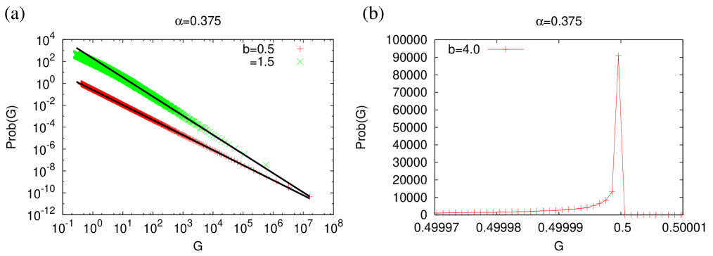
Figure 5: Illustrating the validity of the behavior (28) of the probability distribution ${\rm Prob}(G)$ for three representative values of $b$ at $\alpha=0.375$. The values of $G$ are computed using Eq. (21). The data for $b=1.5$ have been scaled up by a factor of $300$ for convenience of display. The black lines denote analytical predictions, namely, (i) for $b<2$, a power-law decay with exponent $(1+\alpha)$ for $0<b<1$, and exponent $(1+\nu)$ for $1<b<2$, and (ii) for $b>2$, a unit step function.

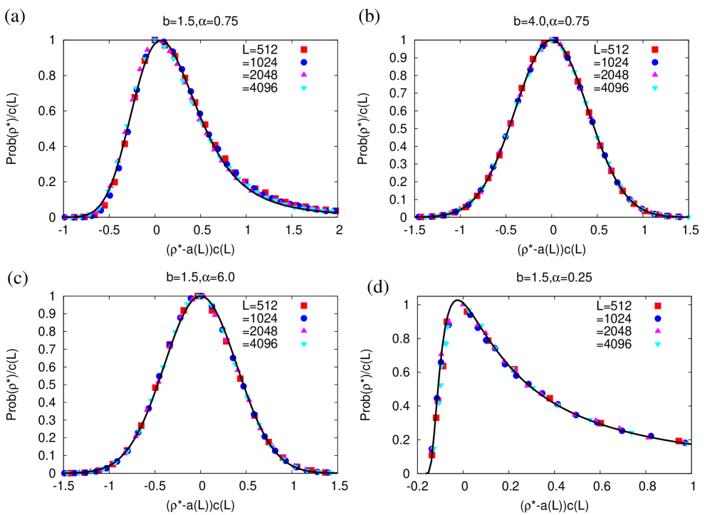
Figure 6: Scaling plots for the probability distribution ${\rm Prob}(\rho^{\star})$ for four representative values of the set $(b,\alpha)$, with $\rho^{\star}$ computed using Eq. (19). Here, the scaling factors are $c(L)={\rm Prob}^{\rm max}(\rho^{\star})$, the maximum value of the distribution, and $a(L)$ the corresponding value of $\rho^{\star}$. (a) and (b) stand for cases where the system supports condensate formation (see condition (18)), and $\rho^{\star}$ coincides with the critical density $\rho_{c}$. (c) and (d) denote cases where the system does not support condensation. The black lines denote analytical predictions, namely, (i) for $b=1.5,\alpha=0.75$ (giving $\nu=1.5$), the inverse Fourier transform of the function $\exp[-|c_{0}k|^{\nu}(1-i\beta\leavevmode\nobreak\ {\rm sgn}(k)\Phi)]$, with $\Phi\equiv\tan(\pi\nu/2)$, $\beta=0.995$, $c_{0}=0.28$, which has been shifted by an amount equal to $0.39$ to fit the data, (ii) for $b=4.0,\alpha=0.75$ and $b=1.5,\alpha=6.0$, a Gaussian with zero mean and variance equal to $1/(2\pi)$, and (iii) for $b=1.5,\alpha=0.25$ (giving $\nu=0.5$), the so-called Lévy distribution $f(x)=\sqrt{c_{0}/(2\pi)}\exp[-c_{0}/(2(x-\mu))]/(x-\mu)^{3/2}$; $c_{0}=0.45$ and $\mu=-0.175$.

Invoking the results on stable distributions discussed above, we may deduce the behavior of ${\rm Prob}(\rho^{\star})$ for different range of values of $b$ by using Eqs. (19) and (28).

1. $0<b<1$: Here, ${\rm Prob}(\rho^{\star})$ is a Lévy-stable distribution with a tail decaying as a power law with exponent $(1+\alpha)$ for values of $\alpha$ in the range $0<\alpha<2$ and is a Gaussian distribution for $\alpha\geq 2$. The mean is finite for $\alpha>1$.

2. $1<b<2$: In this case, ${\rm Prob}(\rho^{\star})$ is a Lévy-stable distribution with a tail decaying as a power law with exponent $(1+\nu)$ for values of $\nu$ in the range $0<\nu<2$, that is, provided $\alpha<4-2b$. On the other hand, for $\alpha\geq 4-2b$, the distribution is a Gaussian. The mean $\rho^{\star}$ is finite for $b+\alpha>2$.

3. $b>2$: In this regime, ${\rm Prob}(G)$ has a finite variance, implying that ${\rm Prob}(\rho^{\star})$ is a Gaussian; the mean is of course finite.

Thus, the condition $b+\alpha>2$ ensures a finite value of the mean $\rho^{\star}$, a condition we derived earlier, see Eq. (25), based on an analysis of the disorder-average $\langle\rho^{\star}\rangle$ defined in Eq. (20).

As a function of the system size $L$, the probability distribution ${\rm Prob}(\rho^{\star})$ has the scaling form (see Fig. 6):

$${\rm Prob}(\rho^{\star})\sim c(L){\mathcal{G}}\Big{[}\Big{(}\rho^{\star}-a(L)\Big{)}c(L)\Big{]},$$ (29)

where $c(L)$ is the maximum value of the distribution, while $a(L)$ is the corresponding value of $\rho^{\star}$. The scaling function ${\mathcal{G}}(x)$ has either (a) a Gaussian form, in which case $a(L)$ is independent of $L$, and $c(L)\sim\sqrt{L}$, or, (b) a Lévy-stable form, in which case we have

1. for $0<b<1$: $a(L)\sim L^{1/\alpha-1}$ and $c(L)\sim L^{1-1/\alpha}$ for $0<\alpha<1$, and $a(L)$ independent of $L$ and $c(L)\sim L^{1-1/\alpha}$ for $\alpha\geq 2$,

2. for $1<b<2$: $a(L)\sim L^{1/\nu-1}$ and $c(L)\sim L^{1-1/\nu}$ for $0<\nu<1$, and $a(L)$ independent of $L$ and $c(L)\sim L^{1-1/\nu}$ for $\nu\geq 2$.

4 Numerical studies

In this section, we check our predictions on the existence of a condensate in the RC-ZRP by reporting on results obtained by a direct numerical sampling of its canonical steady state measure for a given realization of the disorder. When relevant, we also perform Monte Carlo (MC) simulations of the RC-ZRP dynamics while starting from the steady state.

The steady state is generated according to the following algorithm. For a given system size $L$ and disorder realization $\{l_{i}\}$, a configuration of the system corresponding to a total $N$ particles is generated by occupying $L-1$ sites independently with $n_{i}$ ($0\leq n_{i}\leq l_{i}$) particles with respective weights $f_{i}(n_{i}|l_{i})$; here, $i=1,2,\ldots,L-1$. The deficit number of particles, $n_{\rm d}\equiv N-\sum_{i=1}^{L-1}n_{i}$, when positive, is accommodated on the last remaining site $i=L$ with the weight $f_{L}(n_{d}|l_{L})$. If the deficit is negative, the configuration is rejected, and the process is repeated all over again. A configuration so generated is run for a typical “equilibration” time of order $L$ before performing any analysis of the data.

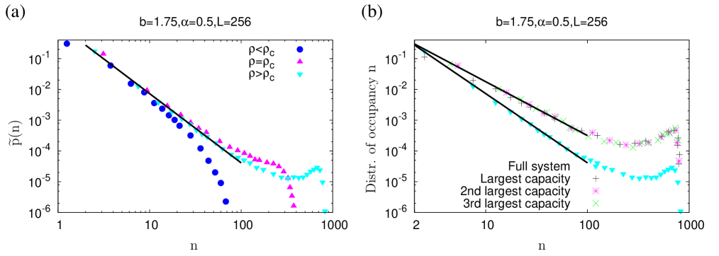
Figure 7: For a fixed disorder realization, (a) shows the occupancy distribution for the full system in the steady state, with densities smaller than, equal to, and larger than the critical density $\rho_{c}$; the density values are $1.0$, $2.28$ and $4.0$, respectively. The system size is $L=256$, and we have taken ${\alpha}=0.5,b=1.75$. The data are obtained by sampling the canonical steady state measure using the algorithm detailed in the text. Below $\rho_{c}$, the distribution shows an exponential decay at large $n$, while at $\rho_{c}$, one has a power-law decay at large $n$ with exponent $(b+\alpha)$, see Eqs. (14) and (27). For $\rho>\rho_{c}$, in addition to the power-law behavior, a bump indicating the presence of a condensate appears. The black line stands for the power-law behavior $\sim n^{-(b+\alpha)}$. (b) shows for $\rho>\rho_{c}$ the occupancy distribution in the steady state for the full system as well as for sites with the largest, the second largest and the third largest capacity. Besides a bump at large $n$ that implies the presence of a condensate, one has a power-law decay at small $n$, with exponent $(b+\alpha)$ for the full system, and with exponent $b$ for individual sites, see Eq. (26).

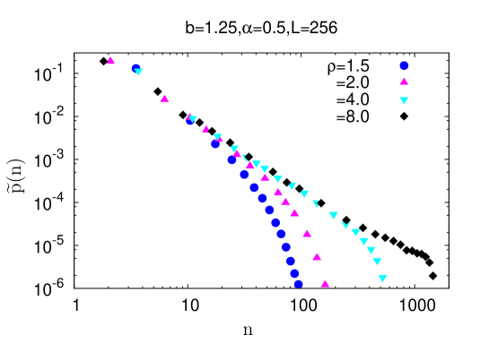
Figure 8: For the same disorder realization, system size and $\alpha$ as in Fig. 7, but for a value of $b$ that does not satisfy the conditions (18) to observe condensation, the figure shows the occupancy distribution for the full system in the steady state at several densities. The data are obtained by sampling the canonical steady state measure using the algorithm detailed in the text. In contrast to Fig. 7(a), the distribution at all densities has an exponential decay at large $n$, and there is no extra peak appearing at high densities that corresponds to a condensate. Here, we have taken $b=1.25$.

Following the above procedure for parameter values $b=1.75,\alpha=0.5$ that satisfy the conditions (18) to observe condensation, Fig. 7(a) shows the results for the occupancy distribution $\widetilde{p}(n)$ for the full system with densities below, at, and above the corresponding critical density $\rho_{c}$, which is computed numerically from Eq. (19). Consistent with the predictions of Section 3, we find that a distribution that decays exponentially for $\rho<\rho_{c}$ goes over to one decaying as a power law at $\rho=\rho_{c}$, which at higher densities develops an additional bump corresponding to the formation of a condensate. The power-law decay exponent equals $(b+\alpha)$, as predicted in Eq. (27). Figure 7(a) is to be contrasted with Fig. 8 obtained for the same disorder realization, system size and $\alpha$, but for a value of $b$ that does not satisfy the conditions (18) to observe condensation; the distribution decays exponentially at all densities.

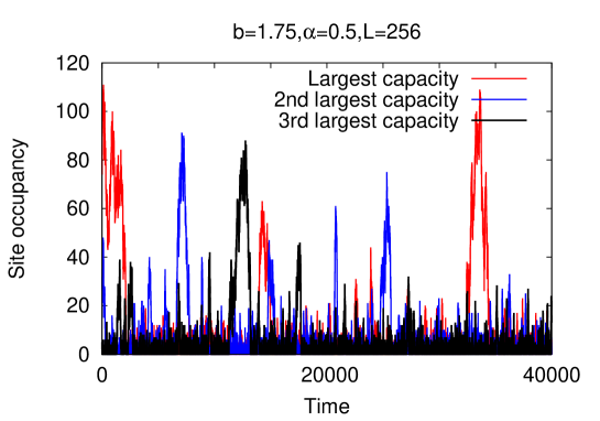
Figure 9: For the same disorder realization and other parameters as in Fig. 7, the figure shows the occupancy at sites with the largest, the second largest and the third largest capacity, all plotted together as a function of time for a single dynamical evolution of the system while starting from the steady state. The data are obtained by performing Monte Carlo simulations of the dynamics starting from a steady state configuration.

4.1 Condensate relocation

In Fig. 7(b), we contrast the single-site occupancy distribution $p_{i}(n|l_{i})$ for large-capacity sites with the occupancy distribution $\widetilde{p}(n)$ for the full system at a density $\rho>\rho_{c}$. The single-site distribution is observed to be the same for the site with the largest capacity (let us denote it by $i_{1}$) and for the ones with the second and the third largest capacity (denoted respectively by indices $i_{2}$ and $i_{3}$). To understand such a behavior, we show in Fig. 9 the results of a MC simulation of the dynamics for the same set of parameter values and the same disorder realization as in Fig. 7. The occupancy at sites $i_{1},i_{2},i_{3}$ have been plotted as a function of time for a single dynamical evolution of the system starting from a steady state configuration. It is evident from the figure that a dip in $n_{1_{1}}$ from a value of $O(L)$ to a value of order $1$ is followed by a rise within a short time in either $n_{i_{2}}$ or $n_{i_{3}}$ from a value of order $1$ to a value of order $L$. This implies that the condensate occupies a single site at almost all times, but does move between certain sites with a relatively small relocation time. The fact that for a given $L$ and a given disorder realization, there are only a finite number ${\cal N}(L,\{l_{i}\})\sim L^{1-\alpha}$ of sites that have capacities equal to or larger than $L$ implies that the condensate can relocate only on this finite subset of sites. A similar relocation dynamics of the condensate on a set of sites whose size grows subextensively with $L$ was observed in a disordered version of the ZRP studied in [29], in which the disorder enters through hop rates. Such a relocation of the condensate on a subset of sites of subextensive size may be contrasted with the situation in the homogeneous ZRP where the condensate can relocate on any of the other $L-1$ sites [36, 37]. In our case, when the condensate has relocated away from one of the sites of this subset to another, the occupancy and fluctuations on the first site become identical to ones in the background that did not contain the condensate. This explains why the single-site distribution for sites $i_{1},i_{2},i_{3}$ are the same. A detailed analysis of the condensate relocation dynamics will be published elsewhere.

5 Conclusions

In this paper, we studied a quenched disordered version of the zero-range process (ZRP), a nonequilibrium system of particles undergoing biased hopping on a one-dimensional periodic lattice. In the model studied, which we refer to as the random capacity zero-range process (RC-ZRP), each site has a finite capacity whereby it can hold only a finite number of particles; we chose the capacities randomly from the Pareto distribution. We obtained the conditions for condensate formation in the RC-ZRP, which derive from an interplay of the capacity distribution with the hop rate. In terms of the power-law exponents $\alpha>0$ and $b>0$ that characterize respectively the capacity distribution and the hop rate, we derived explicit conditions for condensation, namely, $b+\alpha>2$ and $\alpha<1$. Further, we addressed the sample-to-sample variation of the critical density to observe condensation, and demonstrated that the corresponding distribution is either a Gaussian or a Lévy-stable distribution.

Let us remark on the possibility of observing condensation in the RC-ZRP for generalizations of the hop rate $u(n)$ that we studied. Consider, e.g., the choice $u(n)=1+b/n^{\sigma}$, with $\sigma>0$. For $\sigma<1$, the function $G(l)$ in Eq. (19) converges asymptotically to a finite constant for all values of $b$, yielding a finite $\rho^{\star}$. As a result, the system supports condensation for all values of $b$, provided $\alpha<1$, a condition that derives from the desired scaling of $l_{\rm max}$ with system size $L$. On the other hand, for $\sigma>1$, the function $G(l)$ diverges asymptotically for all values of $b$, so that $\rho^{\star}$ is infinite, and consequently, there is no condensate formation in the system.

We sign off by mentioning a possible follow-up of this work. It would be of interest to study the RC-ZRP dynamics in the steady state, and investigate the behavior of time-dependent correlation functions. In this regard, a pertinent issue is to address if and how quenched disorder manifests itself in the behavior of the dynamic universality class at criticality and in the dynamics of condensate relocation, both of which may show significant differences from the homogeneous ZRP [38].

6 Acknowledgments

SG and MB thank the Galileo Galilei Institute for Theoretical Physics, Florence, Italy for hospitality and the INFN for partial support during the completion of this work. MB also acknowledges the hospitality of the Rudolf Peierls Centre for Theoretical Physics, University of Oxford, UK. SG acknowledges fruitful discussions with Martin R. Evans and David Mukamel, and a useful remark on an asymptotic expansion by Pablo Rodriguez-Lopez.

7 Appendix: Characterizing the site capacities – The sum and the maximum

In this appendix, we summarize some features associated with the capacity distribution (1) that are relevant to the understanding of the condensation phenomenon in the RC-ZRP discussed in the main text.

Let us start with discussing the behavior of the mean and the variance of the distribution: they are both finite for $\alpha\geq 2$ and both infinite for $0<\alpha\leq 1$. In the intermediate regime $1<\alpha<2$, the mean is finite while the variance is infinite. For values of $\alpha$ in the range $0<\alpha\leq 2$, the distribution (1) is Lévy-stable: a linear combination of two independently sampled values of $l$ has a distribution identical to $P(l)$, up to location and scale parameters [33, 34, 35]. For $0<\alpha<2$, a Lévy-stable distribution is characterized by a power-law tail with exponent $-(1+\alpha)$; the distribution is a Gaussian for $\alpha=2$.

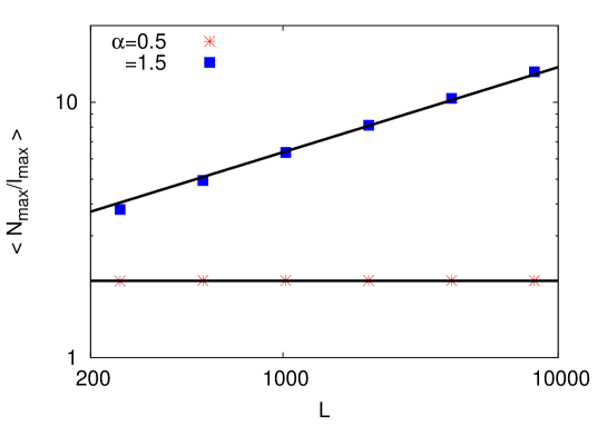
Figure 10: Illustrating the validity of the scaling behavior (32) of the disorder-averaged ratio $\langle N_{\rm max}/l_{\rm max}\rangle$ for two values of $\alpha$, one smaller and one larger than $1$. The data for $\alpha=1.5$ have been scaled down by a factor of $4$ for convenience of display.

Now, let us discuss the scaling with system size $L$ of the largest capacity $l_{\rm max}$ and the largest possible number of particles $N_{\rm max}$ that can be accommodated in the system. For a given $L$ and a given realization $\{l_{i}\}$ of the disorder, we have $l_{\rm max}\equiv{\rm Max}[l_{1},l_{2},\ldots,l_{L}]$ and $N_{\rm max}\equiv\sum_{i=1}^{L}l_{i}$. Since the $l_{i}$’s are sampled independently from the common distribution (1), the probability distribution of $l_{\rm max}$ is

$${\rm Prob}(l_{\rm max})=LP(l_{\rm max})\Big{(}\int_{1}^{l_{\rm max}}dl\leavevmode\nobreak\ P(l)\Big{)}^{L-1}.$$ (30)

In the limit $L\to\infty$, the distribution ${\rm Prob}(l_{\rm max})$ decays for large $l_{\rm max}\gg 1$ as ${\rm Prob}(l_{\rm max})\sim\exp(-Ll_{\rm max}^{-\alpha})$, which implies the following scaling of $l_{\rm max}$ with $L$:

$$l_{\rm max}\sim L^{1/\alpha},$$ (31)

valid for all values of $\alpha>0$.

As to the behavior of $N_{\rm max}$, for $\alpha>1$, when $P(l)$ has a finite mean, one may apply the law of large numbers to deduce that $N_{\rm max}=aL$ in the limit $L\to\infty$, with $a\equiv\int dl\leavevmode\nobreak\ lP(l)$ finite. For $0<\alpha\leq 1$, on the other hand, the mean of $P(l)$ is infinite, the law of large numbers breaks down, and $N_{\rm max}$ is dominated by contributions from capacities of order $l_{\rm max}$. Thus, we anticipate $N_{\rm max}\sim L^{1/\alpha}$, which would imply

$$\Big{\langle}\frac{N_{\rm max}}{l_{\rm max}}\Big{\rangle}\sim\left\{\begin{array}[]{cc}1&\mbox{for\leavevmode\nobreak\ }0<\alpha\leq 1,\\ L^{1-1/\alpha}&\mbox{for\leavevmode\nobreak\ }\alpha>1.\end{array}\right.$$ (32)

Figure 10 illustrates the validity of the above scaling for representative values of $\alpha$. In fact, the full distribution of the ratio $N_{\rm max}/l_{\rm max}$ is known (see [34], page 465), which leads to

$$\Big{\langle}\frac{N_{\rm max}}{l_{\rm max}}\Big{\rangle}=\frac{\alpha}{1-\alpha};\leavevmode\nobreak\ \leavevmode\nobreak\ 0<\alpha<1.$$ (33)

The above result is confirmed in Fig. 10. Note that Eq. (32) suggests that there are several sites other than the site with capacity $l_{\rm max}$ which have capacities of order $L^{1/\alpha}$.

References

- [1] F. Spitzer, Adv. Math. 5, 246 (1970).
- [2] M. R. Evans, Braz. J. Phys. 30, 42 (2000).
- [3] M. R. Evans and T. Hanney, J. Phys. A: Math. Gen. 38, R195 (2005).
- [4] C. Godrèche, in Lecture Notes in Physics (Springer-Verlag, Berlin, 2007), Vol. 716; also e-print:arXiv:cond-mat/0604276.
- [5] G. Tripathy and M. Barma, Phys. Rev. Lett. 78, 3039 (1997).
- [6] G. Tripathy and M. Barma, Phys. Rev. E 58, 1911 (1998).
- [7] J. Török, Physica A 355, 374 (2005).
- [8] D. Chowdhury, L. Santen, and A. Schadschneider, Phys. Rep. 329, 199 (2000).
- [9] Z. Burda, D. Johnston, J. Jurkiewicz, M. Kaminski, M. A. Novak, G. Papp, and I. Zahed, Phys. Rev. E 65, 026102 (2002).
- [10] B. Schmittmann and R. K. P. Zia, in Phase Transitions and Critical Phenomena, edited by C. Domb and J. L. Lebowitz (Academic, London, 1995), Vol. 17.
- [11] R B Stinchcombe, Adv. Phys. 50, 431 (2001).
- [12] G. M. Schüz, in Phase Transitions and Critical Phenomena, Vol. 19, edited by C. Domb and J. L. Lebowitz (Academic, London, 2001).
- [13] M. Barma, Physica A 372, 22 (2006).
- [14] J. Krug and P. A. Ferrari, J. Phys. A: Math. Gen. 29, L465 (1996).
- [15] M. R. Evans, Europhys. Lett. 36, 13 (1996).
- [16] R. Juhász, L. Santen, and F. Iglói, Phys. Rev. Lett. 94, 010601 (2005).
- [17] R. Juhász, L. Santen, and F. Iglói, Phys. Rev. E 72, 046129 (2005).
- [18] S. R Masharian and F. H. Jafarpour, Int. J. Mod. Phys. B 26, 1250044 (2012).
- [19] J. Krug, Braz. J. Phys. 30, 97 (2000).
- [20] M. Barma and K. Jain, Pramana - J. Phys. 58, 409 (2002).
- [21] K. Jain and M. Barma, Phys. Rev. Lett. 91, 135701 (2003).
- [22] R. J. Harris and R. B. Stinchcombe, Phys. Rev. E 70, 016108 (2004).
- [23] A. G. Angel, M. R. Evans, and D. Mukamel, J. Stat. Mech. P04001 (2004).
- [24] C. Enaud and B. Derrida, Europhys. Lett. 66, 83 (2004).
- [25] M. R. Evans, T. Hanney, and Y. Kafri, Phys. Rev. E 70, 066124 (2004).
- [26] B. Waclaw, L. Bogacz, Z. Burda, and W. Janke, Phys. Rev. E 76, 046114 (2007).
- [27] S. Grosskinsky, P. Chleboun, and G. M. Schütz, Phys. Rev. E 78, 030101(R) (2008).
- [28] L. C. G. del Molino, P. Chleboun, and S Grosskinsky, J. Phys. A: Math. Theor. 45, 205001 (2012).
- [29] C. Godrèche and J. M. Luck, J. Stat. Mech. P12013 (2012).
- [30] M. Barma and R. Ramaswamy, in Non-Linearity and Breakdown in Soft Condensed Matter, edited by B. K. Chakrabarti, K. K. Bardhan, and A. Hansen (Springer, Berlin, 1993).
- [31] G. Schütz, R. Ramaswamy, and M. Barma, J. Phys. A 29, 837 (1996).
- [32] A. Ryabov, Phys. Rev. E 89, 022115 (2014).
- [33] W. Feller, An Introduction to Probability Theory and Its Applications, (Wiley, New Jersey, 1971), Vol. I.
- [34] W. Feller, An Introduction to Probability Theory and Its Applications, (Wiley, New Jersey, 1971), Vol. II.
- [35] B. V. Gnedenko and A. N. Kolmogorov, Limit Distributions for Sums of Independent Random Variables, (Addison-Wesley, Cambridge, Massachussetts, 1954).
- [36] C. Godrèche and J. M. Luck, J. Phys. A 38, 7215 (2005).
- [37] C. Landim, Commun. Math. Phys. 330, 1 (2014).
- [38] S. Gupta, M. Barma, and S. N. Majumdar, Phys. Rev. E 76, 060101(R) (2007).