Experimental violation of a Bell-like inequality with optical vortex beams

Abstract

Optical beams with topological singularities have a Schmidt decomposition. Hence, they display features typically associated with bipartite quantum systems; in particular, these classical beams can exhibit entanglement. This classical entanglement can be quantified by a Bell inequality formulated in terms of Wigner functions. We experimentally demonstrate the violation of this inequality for Laguerre-Gauss (LG) beams and confirm that the violation increases with increasing orbital angular momentum. Our measurements yield negativity of the Wigner function at the origin for $\mathrm{LG}_{10}$ beams, whereas for $\mathrm{LG}_{20}$ we always get a positive value.

I Introduction

Entanglement is usually presented as one of the weirdest features of quantum theory that depart strongly from our common sense Schrödinger (1935). Since the seminal work of Einstein, Podolsky, and Rosen (EPR) Einstein et al. (1935), countless discussions on this subject have popped up Horodecki et al. (2009).

A major step in the right direction is due to Bell Bell (1964), who formulated the EPR dilemma in terms of an inequality which naturally led to a falsifiable prediction. Actually, it is common to use an alternative formulation, derived by Clauser, Horne, Shimony and Holt (CHSH) Clauser et al. (1969), which is better suited for realistic experiments.

The main stream of research Brunner et al. (2014); Werner and Wolf (2001) settled the main concepts of this topic in the realm of quantum physics. However, in recent years a general consensus has been reached on the fact that entanglement is not necessarily a signature of the quantumness of a system. Actually, as aptly remarked in RefE. Töppel et al. (2014), one should distinguish between two types of entanglement: between spatially separated systems (inter-system entanglement) and between different degrees of freedom of a single system (intra-system entanglement). Inter-system entanglement occurs only in truly quantum systems and may yield to nonlocal statistical correlations. Conversely, intra-system entanglement may also appear in classical systems and cannot generate nonlocal correlations Brunner et al. (2005); for this reason, it is often dubbed as “classical entanglement”. Since its introduction by Spreeuw Spreeuw (1998), this notion has been employed in a variety of contexts Ghose and Mukherjee (2014).

Classical entanglement has allowed to test Bell inequalities with classical wave fields. The physical significance of this violation is not linked to quantum nonlocality, but rather points to the impossibility of constructing such a beam using other beams with uncoupled degrees of freedom. However, all the experiments conducted thus far to observe this violation have involved only discrete variables, such as spin and beam path of single neutrons Hasegawa et al. (2003), polarization and transverse modes of a laser beam Souza et al. (2007); Simon et al. (2010); Qian and Eberly (2011); Gabriel et al. (2011); Qian et al. , different transverse modes propagating in multimode waveguides Fu et al. (2004), polarization of two classical fields with different frequencies Lee and Thomas (2002), orbital angular momentum Goyal et al. (2013); Chowdhury et al. (2013), and polarization and spatial parity Kagalwala et al. (2013).

In this paper, we continue the analysis of this classical entanglement by focusing on the simple but engaging example of vortex beams. To this end, in Sec. II we revisit a decomposition of Laguerre-Gauss (LG) beams in the Hermite-Gauss (HG) basis that can be rightly interpreted as a Schmidt decomposition. This immediately suggests that many ideas ensuing from the quantum world may be applicable to these beams as well. In particular, in Sec. III we address the inseparability of the LG modes using a CHSH violation that we quantify in terms of the associated Wigner function. As this distribution can be understood as a measure of the displaced parity, in Sec. IV we discuss an experimental realization which nicely agrees with the theoretical predictions. Finally, our conclusions are summarized in Sec. V.

II Optical vortices and Schmidt decomposition

It is well known that the beam propagation along the $z$ direction of a monocromatic scalar field of frequency $\omega$; i.e., $E(\mathbf{r},t)=\mathcal{E}(\mathbf{r})\exp[-i(\omega t-kz)]$, is governed by the paraxial wave equation

$$\frac{\partial\mathcal{E}}{\partial z}=-\frac{\lambdabar}{2}\left(\frac{\partial^{2}}{\partial x^{2}}+\frac{\partial^{2}}{\partial y^{2}}\right)\mathcal{E}\,,$$ (1)

with $\lambdabar=\lambda/2\pi$ and $\lambda$ is the wavelength. Equation (1) is formally identical to the Schrödinger equation for a free particle in two dimensions, with the obvious identifications $t\mapsto z$, $\psi\mapsto\mathcal{E}$, and $\hbar\mapsto\lambdabar$.

Any optical beam can be thus expressed as a superposition of fundamental solutions of Eq. (1). In Cartesian coordinates, a natural orthonormal set is given by the Hermite-Gauss (HG) modes:

$$\mathrm{HG}_{mn}(x,y)=\sqrt{\frac{2}{\pi n!m!2^{n+m}}}\left(\frac{1}{w}\right)H_{m}\left(\frac{\sqrt{2}x}{w}\right)H_{n}\left(\frac{\sqrt{2}y}{w}\right)$$

$$\times\exp\left(-\frac{x^{2}+y^{2}}{w^{2}}\right),$$ (2)

where $w$ is the beam waist, and $H_{m}$ are the Hermite polynomials. Note that we are restricting ourselves to the plane $z=0$, since we are not interested here in the evolution.

For cylindrical symmetry, it is convenient to use the set of Laguerre-Gauss (LG) modes, which contain optical vortices with topological singularities; they read

$$\mathrm{LG}_{mn}(r,\varphi)=\sqrt{\frac{2}{\pi m!n!}}\min(m,n)!(-1)^{\min(m,n)}\left(\frac{1}{w}\right)$$

$$\times\left(\frac{\sqrt{2}r}{w}\right)^{|m-n|}\!\!L_{\min(m,n)}^{|m-n|}\left(\frac{2r^{2}}{w^{2}}\right)\exp\left(-\frac{r^{2}}{w^{2}}\right)\exp[i(m-n)\varphi]\,,$$ (3)

where $L_{p}^{|\ell|}(x)$ are the generalized Laguerre polynomials. A word of caution seems to be in order: usually, these modes are presented in terms of two different indices: the azimuthal mode index $\ell=m-n$, which is a topological charge giving the number of $2\pi$-phase cycles around the mode circumference, and $p=\min(m,n)$ is the radial mode index, which is related to the number of radial nodes Karimi et al. (2014). However, the form (3) will be advantageous in what follows.

The crucial observation is that the LG modes can be represented as superpositions of HG modes, and viceversa. This can be compactly written down as Beijersbergen et al. (1993)

$$\mathrm{LG}_{mn}(\rho,\varphi)=\sum_{k=0}^{m+n}B_{mn}^{k}\,\mathrm{HG}_{m+n-k,k}(x,y)$$ (4)

where the coefficients are

$$B_{mn}^{k}=\sqrt{\frac{k!(m+n-k)!}{m!n!2^{n+m}}}\frac{(-i)^{k}}{k!}\frac{d^{k}}{dt^{k}}\left.[(1-t)^{m}(1+t)^{n}]\right|_{t=0}.$$ (5)

This looks exactly the same as a Schmidt decomposition for a bipartite quantum system. It is nothing but a particular way of expressing a vector in the tensor product of two inner product spaces Peres (1993). Alternatively, it can be seen as another form of the singular-value decomposition Stewart (1993), which identifies the maximal correlation directly. In quantum information, the Schmidt coefficients $B_{mn}^{k}$ convey complete information of the entanglement Agarwal and Banerji (2002). Here, we intend to assess entanglement in LG beams via the violation of suitably formulated Bell inequalities.

III CHSH violation for Laguerre-Gauss modes

The traditional form of the CHSH inequality applies to dichotomic discrete variables. For continuous variables, the sensible formulation is in terms of the Wigner function, which for a classical beam reads

$$W(\mathbf{x},\mathbf{p})=\frac{1}{\lambdabar^{2}\pi^{2}}\int d^{2}\mathbf{x}^{\prime}\,e^{2i\mathbf{p}\cdot\mathbf{x}^{\prime}/\lambdabar}\langle E^{\ast}(\mathbf{x}-\mathbf{x}^{\prime})E(\mathbf{x}+\mathbf{x}^{\prime})\rangle\,,$$ (6)

the angular brackets denoting statistical average. Although originally introduced to represent quantum mechanical phenomena in phase space Wigner (1932), the Wigner distribution was established in optics Walther (1968) to relate partial coherence with radiometry. Since then, a great number of applications of this function have been reported Bastiaans (2009); Galleani and Cohen (2002); Dragoman (1997); Mecklenbraüker and Hlawatsch (1997); Alonso (2011). Note that $W$ has the dimensions of an intensity and it yields a description displaying both the position and the momentum (which in the paraxial approximation has the significance of a scaled angular coordinate) of the intensity of the wave field: in fact, one easily proves that

$$\displaystyle\int W(\mathbf{x},\mathbf{p})\,d\mathbf{p}=I(\mathbf{x})\equiv\langle E^{\ast}(\mathbf{x})E(\mathbf{x}\rangle\,,$$

(7)

$$\displaystyle\frac{1}{\lambdabar^{2}\pi^{2}}\int W(\mathbf{x},\mathbf{p})\,d\mathbf{x}=I(\mathbf{p})\equiv\langle E^{\ast}(\mathbf{p})E(\mathbf{p})\rangle\,,$$

with

$$E(\mathbf{p})=\frac{1}{\lambdabar^{2}\pi^{2}}\int E(\mathbf{x})\,\exp(i\mathbf{p}\cdot\mathbf{x}/\lambdabar)\,d\mathbf{x}\,.$$ (8)

Thus, the marginals of the Wigner function are the intensity distributions in $\mathbf{x}$ or $\mathbf{p}$ space, respectively.

The CHSH inequality can now be stated in terms of the Wigner function as Banaszek and Wódkiewicz (1999)

$$B=\frac{\pi^{2}}{4}|W(\alpha,\beta)+W(\alpha,\beta^{\prime})+W(\alpha^{\prime},\beta)-W(\alpha^{\prime},\beta^{\prime})|<2,$$ (9)

where $\alpha=(x,p_{x})/\sqrt{2}$ and $\beta=(y,p_{y})/\sqrt{2}$. This also follows from the work of Gisin Gisin (1991), who formulated a Bell inequality for the set of observables with the property $\hat{O}^{2}=\openone$: as we shall see, the Wigner function appears as the average value of the parity, whose square is unity. Reference Chowdhury et al. (2013) presents a detailed study of the violations of (9).

For the state $\mathrm{LG}_{mn}$, the normalized Wigner function can be written as Simon and Agarwal (2000)

$$W_{mn}^{\mathrm{LG}}(X,P_{X};Y,P_{Y})=\frac{(-1)^{m+n}}{\pi^{2}}\exp(-4Q_{0})$$

$$\times L_{m}[4(Q_{0}+Q_{2})]L_{n}[4(Q_{0}-Q_{2})]\,,$$ (10)

where

$$Q_{0}=\frac{1}{4}(X^{2}+Y^{2}+P_{X}^{2}+P_{Y}^{2})\,,\qquad Q_{2}=\frac{1}{2}(XP_{Y}-YP_{X})\,,$$ (11)

and we have rescaled the variables as $x\mapsto(w/\sqrt{2})X$ and $p_{x}\mapsto(\sqrt{2}\lambdabar/w)~{}P_{X}$ (and analogously for the $y$ axis). Let us first look at the simple case of the mode $\mathrm{LG}_{10}$, which reduces to

$$W^{\mathrm{LG}}_{10}(X,P_{X};Y,P_{Y})=\frac{1}{\pi^{2}}\exp(-P_{X}^{2}-P_{Y}^{2}-X^{2}-Y^{2})$$

$$\times[(P_{X}-Y)^{2}+(P_{Y}+X)^{2}-1]\,.$$ (12)

The two measurement settings on one side are chosen to be $\alpha=(X=0,P_{X}=0)$ and $\alpha^{\prime}=(X^{\prime}=X,P_{X}^{\prime}=0)$, and the corresponding settings on the other side are $\beta=(Y=0,P_{Y}=0)$ and $\beta^{\prime}=(Y^{\prime}=0,P_{Y}^{\prime}=P_{Y})$ Zhang et al. (2007), for which the Bell sum is

$$B=e^{-P_{Y}^{2}}(P_{Y}^{2}-1)+e^{-X^{2}}(X^{2}-1)$$

$$-e^{-(P_{Y}^{2}+X^{2})}[(P_{Y}+X)^{2}-1]-1\,.$$ (13)

Upon maximization with respect to $X$ and $P_{Y}$, we obtain the maximum Bell violation, $|B_{\mathrm{max}}|\simeq 2.17$, which happens for the choices $X\simeq 0.45,~{}P_{Y}\simeq 0.45$ Chowdhury et al. (2013). For comparison, note that the maximum Bell violation in quantum mechanics through the Wigner function for the two-mode squeezed vacuum state using similar settings is given by $|B_{\mathrm{max}}^{\mathrm{QM}}|\simeq 2.19$ Banaszek and Wódkiewicz (1999).

The Bell violation may be further optimized by a more general choice of settings than those used here. For example, maximizing it with respect to the parameters $\alpha=(X,P_{X})$, $\alpha^{\prime}=(X^{\prime},P_{X}^{\prime})$, $\beta=(Y,P_{Y})$, $\beta^{\prime}=(Y^{\prime},P_{Y}^{\prime})$, one obtains the absolute maximum Bell violation, $|B_{\max}|=2.24$ and occurs for the choices $X\simeq-0.07,~{}P_{X}\simeq 0.05,~{}X^{\prime}\simeq 0.4,~{}P_{X}^{\prime}\simeq-0.26,~{}Y\simeq-0.05,~{}P_{Y}\simeq-0.07,~{}Y^{\prime}\simeq 0.26,~{}P_{Y}^{\prime}\simeq 0.4$. The violation also increases with higher orbital angular momentum. This increase with $n$ is analogous to the enhancement of nonlocality in quantum mechanics for many-particle Greenberger-Horne-Zeilinger states Mermin (1990).

IV Experimental results

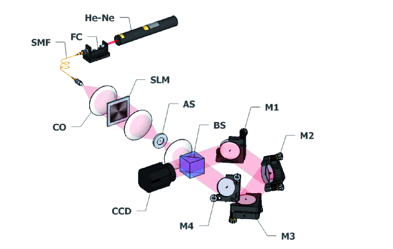
Figure 1: (Color online) Scheme of the Bell measurement. The abbreviations are as follows: He-Ne: laser source, FC: fiber coupler, SMF: single mode fiber, CO: collimation optics, SLM: spatial light modulator, AS: aperture stop, BS: beam splitter, M1-M4: mirrors, CCD: camera

We have carried a direct measurement of the Bell sums for optical beams with different amount of nonlocal correlations. To understand the measurement, we recall that the Wigner function in quantum optics is often regarded as the average of the displaced parity operator Royer (1977). At the classical level, we can consider the field amplitudes $\mathcal{E}(X,Y)$ as vectors in the Hilbert space of complex-valued functions that are square integrable over a transverse plane. In this space we define linear Hermitian operators

$$\hat{X}:\mathcal{E}(X,Y)\mapsto X\mathcal{E}(X,Y)\,,\qquad\hat{P}_{x}:\mathcal{E}(X,Y)\mapsto-i\frac{\partial}{\partial X}\mathcal{E}(X,Y)\,,$$ (14)

and analogous ones for the $Y$ variable. Formally, these operators satisfy the canonical commutation relations $[\hat{X},\hat{P}_{X}]=[\hat{Y},\hat{P}_{Y}]=i$. Therefore, the unitary parity operator is

$$\hat{\Pi}_{X}\,\hat{X}\,\hat{\Pi}_{X}=-\hat{X}\,,\qquad\hat{\Pi}_{X}\,\hat{P}_{X}\,\hat{\Pi}_{X}=-\hat{P}_{X}\,,$$ (15)

and changes $\mathcal{E}(X,Y)$ into $\mathcal{E}(-X,Y)$. The displacement operators are

$$\hat{D}(X,P_{X})=\exp[i(P_{X}\hat{X}-X\hat{P}_{X})]\,.$$ (16)

Indeed, with these notations we have

$$W(X,P_{x};Y,P_{y}) =$$

$$\frac{4}{\pi^{2}}\langle\hat{D}(X,P_{x})\hat{\Pi}_{X}\hat{D}^{\dagger}(X,P_{x})\,\hat{D}(Y,P_{y})\hat{\Pi}_{Y}\hat{D}^{\dagger}(Y,P_{y})\rangle\,.$$ (17)

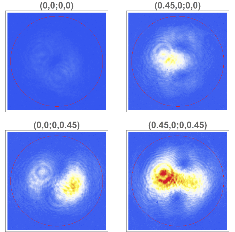
Figure 2: (Color online) Snapshots of the CCD camera for the state $\mathrm{LG}_{10}$ at the four settings $(X,P_{X};Y,P_{Y})$ indicated. The scans are normalized to the peak intensity among the measurements and the area of interest for the intensity integration is marked by a red circle.

Parity measurement can be, in turn, realized by a common-path interferometer with a Dove prism inserted into the optical path Mukamel et al. (2003). In our setup, sketched in Fig. 1, the prism was substituted with an equivalent four-mirror Sagnac arrangement Smith et al. (2005). The two copies of the input signal obtained after the input beam splitter are transformed by the mirrors so as to make one copy spatially inverted with respect to the other, prior to combining the beams together. The resulting interference pattern is detected by a CCD camera: Figure 2 shows snapshots of the camera for the state $\mathrm{LG}_{10}$ at the four settings indicated. The total intensity witnessing parity of the measured beam is computed by spatial integration and this is proportional to the desired Wigner distribution sample after normalization to the overall intensity.

The target signal beams were prepared with digital holograms created by a spatial light modulator (SLM), which modulated a collimated output of a single mode fiber coupled to a He-Ne laser. We also included a 4$f$-system, with an aperture stop, to filter the unwanted diffraction orders produced by the SLM. To allow for a better flexibility, all the necessary shifts in the $X$, $Y$, $P_{X}$, and $P_{Y}$ variables were incorporated into the SLM, so that each Bell measurement was associated with a separate hologram.

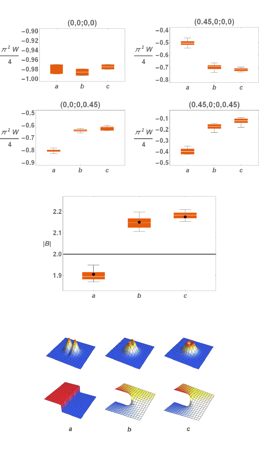
Figure 3: (Color online) Experimental results for three different optical beams: a) $\mathrm{HG}_{10}$, b) $0.4\,\mathrm{HG}_{10}+i0.6\,\mathrm{HG}_{01}$, and c) $\mathrm{LG}_{10}$. At the top, we plot $\frac{\pi^{2}}{4}W(X,P_{X};Y,P_{Y})$ at the values $(X,P_{X};Y,P_{Y})$ indicated for each one. The next plot shows the measured Bell sums, all reported with $75\%$ and $25\%$ quartile (orange boxes) and the minimal and maximal measured values (error bars). The theoretical values $(-1.91,-2.15,-2.17)$ are the dots and the black bar is at $|B|=2$, which delimites the classically entangled states. The theoretical amplitude (top) and phase (bottom) distributions of the measured beams are plotted bellow the chart.

The measured beams were coherent superpositions of Hermite-Gaussian beams in the form $a\,\mathrm{HG}_{10}+ib\,\mathrm{HG}_{01}$ with $\{a=1,\,b=0\}$, $\{a=0.4,\,b=0.6\}$ and $\{a=0.5,\,b=0.5\}$, respectively. The first and the third are thus a pure Hermite-Gaussian beam and a pure Laguerre-Gaussian vortex beam, respectively. For all the beams we used the settings $X\simeq 0.0,~{}P_{X}\simeq 0.0,~{}X^{\prime}\simeq-0.45,~{}P_{X}^{\prime}\simeq 0.0,~{}Y\simeq 0.0,~{}P_{Y}\simeq 0.0,~{}Y^{\prime}\simeq 0.0,~{}P_{Y}^{\prime}\simeq-0.45$ for the evaluation of the Bell sums. The theoretical values of the Bell sums for these are $(-1.91,-2.15,-2.17)$, respectively.

Each measurement was repeated many times with slightly different readings, due to laser intensity instabilities and CCD noise. These effects manifest as measurement errors, which can be estimated from the sample statistics. As the parity measurement requires to normalize the total measured intensity of the interference pattern with respect to the input beam intensity, a separate reading of the input beam intensity was performed. For each optical beam, the mean value of the Bell sum is reported. The results are summarized in Fig. 3. The Bell correlations grow with the coupling between the basis $\mathrm{HG}_{10}$ and $\mathrm{HG}_{01}$ modes, with statistically significant violation of CHSH inequality by the second and third beams, as theoretically predicted.

We also show the measured values of the Wigner function. For both, $\mathrm{HG}_{10}$ and $\mathrm{LG}_{10}$ modes, the values of $\pi^{2}W(0,0;0,0)$ are quite close to $-1$. For classical beams, ours is one of the few measurements on the negativity of the Wigner function, though it has to be anticipated from the corresponding results in quantum optics Schleich (2000). We note that very early, March and Wolf Marchand and Wolf (1974) had constructed an example of a classical source which exhibited negative Wigner function.

Finally, we have checked the violation of CHSH inequality for the beam $\mathrm{LG}_{20}$. A beam with higher topological charge is more sensitive to setup imperfections, hence the Bell sum variation is significantly larger than in the case of $\mathrm{LG}_{10}$. On the other hand, as shown in Fig. 4, the increasing of the Bell sum for higher orbital angular momentum is clearly demonstrated: the theoretical value for $\mathrm{LG}_{20}$ is $-2.24$, which agrees pretty well with the experimental results. . Note that the Wigner function at the origin for the $\mathrm{LG}_{20}$ beam is positive, as expected.

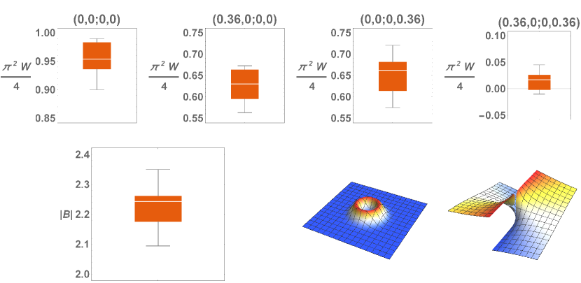
Figure 4: (Color online) Experimental results for the beam $\mathrm{LG}_{20}$, as presented in Fig. 3. The values of $(X,0;0,P_{Y})$ are also indicated. The Bell sum variation is significantly larger than in the case of $LG_{10}$. The plots on the right bottom panel are the amplitude and phase of $\mathrm{LG}_{20}$.

V Concluding remarks

In short, we have presented an experimental study of nonlocal correlations in classical beams with topological singularities Chowdhury et al. (2013). These correlations between modes are manifested through the violation of a CHSH inequality, which we have detected via direct parity measurements. Such a violation is shown to increase with the value of orbital angular momentum of the beam. As a byproduct of our measurements, we obtain negativity of the Wigner function at certain points in phase space for the $\mathrm{HG}_{10}$ and $\mathrm{LG}_{10}$ beams. Note that this has implications for similar studies with electron beams, for which vortices have been reported Verbeeck et al. (2010); McMorran et al. (2011).

Though entanglement here does not bear any paradoxical meaning, such as “spooky action on the distance”, it still represents a potential resource for classical signal processing. It might be expected that future applications of quantum information processing can be tailored in terms of classical light: the research presented in this work explores one of those options.

Furthermore, our results are relevant not only for a correct understanding of “classical entanglement”, but also for bringing out different statistical features of the optical beams, since it provides an alternative paradigm to the well developed optical coherence theory.