Numerical solutions of Einstein’s equations for cosmological spacetimes with spatial topology $\mathbb{S}^{3}$ and symmetry group $\mathrm{U(1)}$

Abstract

In this paper we consider the single patch pseudo-spectral scheme for tensorial and spinorial evolution problems on the $2$-sphere presented in [4, 3] which is based on the spin-weighted spherical harmonics transform. We apply and extend this method to Einstein’s equations and certain classes of spherical cosmological spacetimes. More specifically, we use the hyperbolic reductions of Einstein’s equations obtained in the generalized wave map gauge formalism combined with Geroch’s symmetry reduction, and focus on cosmological spacetimes with spatial $\mathbb{S}^{3}$-topologies and symmetry groups $\mathrm{U(1)}$ or $\mathrm{U(1)}\times\mathrm{U(1)}$. We discuss analytical and numerical issues related to our implementation. We test our code by reproducing the exact inhomogeneous cosmological solutions of the vacuum Einstein field equations obtained in [7].

1 Introduction

For many interesting problems, in particular in general relativity, spherical topologies $\mathbb{S}^{2}$ or $\mathbb{S}^{3}$ play an important role. In the context of cosmological models the spherical Friedman-Robertson-Walker models, the Bianchi IX or the Kantowski-Sachs models are particularly important examples. The main difficulty for the numerical (and analytical) treatment of spherical manifolds is the fact that these manifolds cannot be covered globally by a single regular coordinate patch, and therefore the coordinate description of any smooth tensorial quantity inevitably breaks down somewhere. In the literature this problem is often referred to as the pole problem since in standard polar coordinates for the $2$-sphere $\mathbb{S}^{2}$ these issues appear at the poles. Many approaches have been tried to deal with this issue, see for instance [22, 30] and references therein. In earlier work [4, 3], we have presented a numerical framework which applies to situations which involve the $2$-sphere. The main idea of this approach is to implement and extend the algorithm introduced by Huffenberger and Wandelt (HWT) in [29] to compute a transform for functions of given spin-weight $s$ on the $2$-sphere in terms of spin-weighted spherical harmonics. The concepts of the spin-weight, the so-called eth-operators and of spin-weighted spherical harmonics were introduced originally in [36] and shall be reviewed in Section 2.3 below. As a consequence of this formalism, our code is (pseudo-)spectral in space; time evolutions are performed with the method of lines and standard ODE integrators (see below). We also point the reader to alternative implementations of this and similar formalisms in [25, 2, 10].

In our earlier work [4, 3], we have studied simple evolution problems, like the $2+1$-Maxwell and $2+1$-Dirac equation, on fixed $\mathbb{S}^{2}$-backgrounds as test applications for our numerical infrastructure. The main motivation for this paper now is to apply the same formalism and numerical infrastructure to the much more complicated situation of the full Einstein equations. In this context, $2$-spheres arise in a very natural way. In the asymptotically flat setting for example the spatial manifold $\mathbb{R}\times\mathbb{S}^{2}$ is often considered which allows to address the spherical character of the far zone of the radiation field. In the cosmological setting, which we are interested in here, we can find $\mathbb{S}^{2}$-topologies as a consequence of Geroch’s symmetry reduction [24] (see Section 2.1) when the original spatial manifold has a symmetry. For example this was the basis for the work by Moncrief in [34] and for subsequent papers, and for the work in [6, 7] which shall play a particularly important role in Section 5. Here the spacetimes of interest have spatial $\mathbb{S}^{3}$-topologies and the metrics have a certain spacelike symmetry such that Geroch’s reduction yields the spatial manifold $\mathbb{S}^{2}$. The $3+1$-vacuum Einstein equations thereby become $2+1$-coupled Einstein-scalar field equations. All of this is explained in Section 2.1. Notice that Geroch’s symmetry reduction has also been used to obtain axially symmetric reductions of Einstein’s equations in the asymptotically flat case; see for example [11, 40].

The extraction of suitable evolution and constraint equations from Einstein’s equations is essentially the same problem, both in the original $3+1$ and in the reduced $2+1$-case. We use the generalized wave map formalism [21] (also called generalized harmonic map formalism or simply wave/harmonic map formalism) which can be understood as a covariant version of the more familiar generalized wave/harmonic formalism; the latter was first introduced in [21] in order to generalize the original harmonic/wave gauge considered in [18]. We summarize the wave map formalism in Section 3.1. It turns out that in combination with the spin-weight formalism all singular terms caused by the singular polar coordinate chart of the $2$-sphere can be completely eliminated. This had already been observed for the simpler equations considered in [4, 3]. Notice that generalized wave gauges have been used extensively in the literature in various contexts, see for instance [23].

The numerical results in this paper are obtained using the spin-weighted spherical harmonics transform in [4, 3]. The underlying Fourier transform is $2$-dimensional as it applies to functions defined on the $2$-dimensional manifold $\mathbb{S}^{2}$. Sometimes however it is interesting to restrict to special classes of functions on $\mathbb{S}^{2}$ and therefore to derive a specialized, but more efficient version of this transform. In our context we shall be interested in functions on $\mathbb{S}^{2}$ which are invariant under rotations around an axis (in $\mathbb{R}^{3}$), i.e., functions which do not depend on the azimuthal angle $\varphi$ in standard polar coordinates. For such functions, the $2$-dimensional transform is inefficient. In this paper, we therefore also present an efficient implementation of a $1$-dimensional variant of this transform which applies to such axially symmetric functions on $\mathbb{S}^{2}$. The complexity $\mathcal{O}(L^{3})$ of the $2$-dimensional transform is thereby reduced to the complexity $\mathcal{O}(L^{2})$, where $L$ is the band limit of the functions on $\mathbb{S}^{2}$ in terms of the spin weight spherical harmonics. We call this transform the axially symmetric spin-weighted transform. It will be discussed in detail in Section 4.

Finally, Section 5 is devoted to a test application of our numerical approach. We discuss different error sources and how they arise in our implementation. We also study the evolution using the areal gauge and the generalized wave map gauge.

2 Preliminaries

2.1 Geroch’s symmetry reduction

In this section, we give a quick overview of Geroch’s symmetry reduction [24]. Let $M=\mathbb{R}×\Sigma$ be a globally hyperbolic $4$-dimensional spacetime endowed with a metric $g_{ab}$ of signature ($−,+,+,+$) and a global smooth time function $t$ whose level sets are Cauchy surfaces homeomorphic to $\Sigma$. We denote the hypersurfaces given by $t=t_{0}$ for any constant $t_{0}$ by $\Sigma_{t_{0}}$. Each $\Sigma_{t_{0}}$ is homeomorphic to $\Sigma$. To begin with, let $\xi^{a}$ be a smooth space-like Killing vector field on $M$ induced by the smooth effective global action of the group $\mathrm{U(1)}$. We suppose that $\xi^{a}$ is everywhere tangent to the hypersurfaces $\Sigma_{t}$ and define

$$\tilde{\psi}:=g_{ab}\xi^{a}\xi^{b},\quad\tilde{\Omega}_{a}:=\epsilon_{abcd}\>\xi^{b}\mathfrak{D}^{c}\xi^{d}$$ (2.1)

as the norm and the twist of $\xi^{a}$ respectively. The operator $\mathfrak{D}$ is the covariant derivative compatible with the metric $g_{ab}$. Notice that by the Frobenius theorem, the field $\xi^{a}$ is hypersurface orthogonal if and only if $\tilde{\Omega}_{a}=0$. We also define

$$\tilde{h}_{ab}:=g_{ab}−\frac{1}{\tilde{\psi}}\xi_{a}\xi_{b}.$$ (2.2)

It turns out that for vacuum spacetimes $(M,g_{ab})$ with any cosmological constant $\Lambda$ the $1$-form $\tilde{\Omega}_{a}$ is closed. This fact allows us to introduce a local twist potential $\tilde{\omega}$ so that $\tilde{\Omega}_{a}=\mathfrak{D}_{a}\tilde{\omega}$. In fact, $\tilde{\omega}$ is a global potential if $M$ is simply connected as we shall always assume.

Let $S$ be the set of orbits of $\xi^{a}$ on $M$ and consider the map

$$\pi:M\to S,$$

where $\pi$ maps every $p\in M$ to the uniquely determined integral curve of $\xi^{a}$ through $p$. The requirement that $\pi$ is a smooth map induces a differentiable structure on $S$, and hence it can be considered as a smooth manifold. Since $\mathcal{L}_{\xi}\tilde{h}_{ab}=0$, there is a unique smooth Lorentzian metric on $S$ which pulls back to $\tilde{h}_{ab}$ along $\pi$. We write this metric on $S$ as $\hat{h}_{ab}$. For the same reason, there are also unique functions $\psi$, $\omega$ on $S$ which pull back to $\tilde{\psi}$ and $\tilde{\omega}$. It turns out that Einstein’s field equations with cosmological constant $\Lambda$ for $(M,g_{ab})$ imply the following set of equations for $(S,h_{ab},\psi,\omega)$ where

$$h_{ab}:=\psi\hat{h}_{ab}.$$ (2.3)

We call this system the Geroch-Einstein system (GES) and it reads

$$\nabla_{a}\nabla^{a}\psi = \dfrac{1}{\psi}\left(\nabla_{a}\psi\nabla^{a}\psi-\nabla_{a}\omega\nabla^{a}\omega\right)-2\Lambda,$$

$$\nabla_{a}\nabla^{a}\omega = \dfrac{1}{\psi}\nabla^{a}\psi\nabla_{a}\omega,$$ (2.4)

$$R_{ab} = E_{ab}+\dfrac{2\Lambda}{\psi}h_{ab},$$

with

$$E_{ab}=\dfrac{1}{2\psi^{2}}\left(\nabla_{a}\psi\nabla_{b}\psi+\nabla_{a}\omega\nabla_{b}\omega\right),$$ (2.5)

where $R_{ab}$ is the Ricci tensor associated with $h_{ab}$. In fact, the equations for $\psi$ and $\omega$ imply that

$$T_{ab}:=E_{ab}-\dfrac{1}{2}h_{ab}E,$$ (2.6)

is divergence free. It thus plays the role of the energy momentum tensor associated with the two scalar fields $\psi$ and $\omega$ in the $2+1$-dimensional spacetime $S$ with metric $h_{ab}$. As a result, the GES can be interpreted as the equations of 2+1-gravity coupled to two scalar fields $\psi$ and $\omega$ governed by wave-map equations.

Suppose for a moment that $\psi$, $\omega$ and ${h}_{ab}$ are known and that they satisfy Eq. (2.1). Then we can reconstruct a solution $(M,g_{ab})$ of the $3+1$-dimensional Einstein vacuum equation with cosmological constant $\Lambda$ as follows. It turns out that as a consequence of the above equations, the $2$-form

$$\alpha_{ab}=\frac{1}{2\psi^{3/2}}\epsilon_{abc}\Omega^{c}$$

on $S$ is curl-free, i.e.,

$$\nabla_{[a}\alpha_{bc]}=0.$$

We can pull this quantity back to a $2$-form $\tilde{\alpha}$ on $M$ which is also curl-free. This means that there exists, locally, a $1$-form $\tilde{\eta}_{a}$ on $M$ such that

$$\mathfrak{D}_{[a}\tilde{\eta}_{b]}=\tilde{\alpha}_{ab};$$

notice that it is irrelevant here that the Levi-Civita covariant derivative $\mathfrak{D}_{a}$ is not yet known at this stage due to the antisymmetrization. In fact, the $1$-form $\eta_{a}$ is uniquely determined by this equation up to the gradient of a smooth function $f$ and we can use some of the freedom in choosing $f$ to set $\eta_{a}\xi^{a}=1$. Then the metric

$$g_{ab}=\tilde{h}_{ab}+\tilde{\psi}\tilde{\eta}_{a}\tilde{\eta}_{b},$$

where $\tilde{h}_{ab}$ and $\tilde{\psi}$ are the pull-backs of $h_{ab}/\psi$ and $\psi$, respectively, is a solution of the $3+1$ Einstein vacuum equation with cosmological constant, $\Lambda$, and, we find

$$\xi_{a}=g_{ab}\xi^{b}=\psi\eta_{a}.$$

So effectively, the quantities $\psi$, $\omega$ and ${h}_{ab}$ determine the metric $g_{ab}$ up to a total gradient of some function $f$ which fixes the covariant version $\xi_{a}$ of the Killing vector field $\xi^{a}$.

2.2 The $2$- and $3$-spheres

To begin with, we consider the manifold $\mathbb{S}^{3}$ as the submanifold of $\mathbb{R}^{4}$ given by $x_{1}^{2}+x_{2}^{2}+x_{3}^{2}+x_{4}^{2}=1$. We can introduce Euler coordinates $(\theta,\lambda_{1},\lambda_{2})$ on $\mathbb{S}^{3}$

$$\begin{split}x_{1}&=\cos\frac{\theta}{2}\cos\lambda_{1},\quad x_{2}=\cos\frac{\theta}{2}\sin\lambda_{1},\\ x_{3}&=\sin\frac{\theta}{2}\cos\lambda_{2},\quad x_{4}=\sin\frac{\theta}{2}\sin\lambda_{2},\end{split}$$

where $\theta\in(0,\pi)$ and $\lambda_{1},\lambda_{2}\in(0,2\pi)$. Alternatively, we use coordinates $(\theta,{\rho_{1}},{\rho_{2}})$ (which are also referred to as Euler coordinates) with $\theta$ as above and

$$\lambda_{1}=(\rho_{1}+\rho_{2})/2,\quad\lambda_{2}=(\rho_{1}-\rho_{2})/2.$$ (2.7)

Clearly, both sets of Euler coordinates break down at $\theta=0$ and $\pi$. The vector fields $\partial_{\rho_{1}}$ and $\partial_{\rho_{2}}$ are smooth and non-vanishing vector fields on $\mathbb{S}^{3}$ which become parallel at the poles $\theta=0,\pi$.

Similarly we define the manifold $\mathbb{S}^{2}$ as the subset $y_{1}^{2}+y_{2}^{2}+y_{3}^{2}=1$ of $\mathbb{R}^{3}$ and introduce standard polar coordinates

$$y_{1}=\sin\vartheta\cos{\varphi},\quad y_{2}=\sin\vartheta\sin{\varphi},\quad y_{3}=\cos\vartheta.$$

The Hopf map $\pi:\mathbb{S}^{3}\rightarrow\mathbb{S}^{2}$ is

$$(x_{1},x_{2},x_{3},x_{4})\mapsto(y_{1},y_{2},y_{3}) =(2(x_{1}x_{3}+x_{2}x_{4}),2(x_{2}x_{3}-x_{1}x_{4}),x_{1}^{2}+x_{2}^{2}-x_{3}^{2}-x_{4}^{2})$$

$$=(\sin\theta\cos{\rho_{2}},\sin\theta\sin{\rho_{2}},\cos\theta).$$

This is a smooth map which has the coordinate representation

$$\pi:(\theta,{\rho_{1}},{\rho_{2}})\mapsto(\vartheta,\varphi)=(\theta,{\rho_{2}}).$$ (2.8)

Hence, with respect to our coordinates, the Hopf map reduces to a simple projection map. Now, $\mathbb{S}^{3}$ is a principal fiber bundle over $\mathbb{S}^{2}$ with structure group $\mathrm{U(1)}$ whose bundle map is the Hopf map. In fact, if $M=\mathbb{R}\times\mathbb{S}^{3}$ and $\xi^{a}=\partial_{\rho_{1}}^{a}$ is assumed to be a Killing vector (as we will do) then $S=\mathbb{R}\times\mathbb{S}^{2}$ is the space of orbits and $\pi$ the corresponding map in Geroch’s symmetry reduction.

In this paper, we shall employ this relationship between $\mathbb{S}^{3}$ and $\mathbb{S}^{2}$ for our studies of $U(1)$-symmetric fields. Just as a side remark we also mention the case $\Sigma=\mathbb{S}^{1}\times\mathbb{S}^{2}$ which is a trivial bundle over $\mathbb{S}^{2}$. If $\xi^{a}$ agrees with a vector field tangent to the $\mathbb{S}^{1}$-factor and we introduce appropriate coordinates, then the bundle map $\pi:\mathbb{S}^{1}\times\mathbb{S}^{2}\rightarrow\mathbb{S}^{2}$ takes the same coordinate form as Eq. (2.8). In particular, Geroch’s symmetry reduction also yields the space of orbits $S=\mathbb{R}\times\mathbb{S}^{2}$. Hence, almost all techniques which we introduce in this paper, can also be applied to that case.

2.3 The bundle of orthonormal frames over $\mathbb{S}^{2}$ and spin-weighted spherical harmonics

$\mathrm{SO}(3)$ is the bundle of oriented orthonormal frames over $\mathbb{S}^{2}$ with structure group $U(1)$. Given that $\mathrm{SO}(3)$ is double covered by $\mathrm{SU}(2)$ and that the latter is diffeomorphic to $\mathbb{S}^{3}$, the Hopf map $\pi:\mathbb{S}^{3}\rightarrow\mathbb{S}^{2}$ can be identified with the bundle map. The theoretical details are discussed, for example, in [4]. Hence, when we start from the spatial manifold $\mathbb{S}^{3}$, do the symmetry reduction as explained before and therefore arrive at the spatial manifold $\mathbb{S}^{2}$, the manifold $\mathbb{S}^{3}$ “reappears” in a different role, namely as the bundle of orthonormal frames. In practice this means the following: we let $U$ be the dense open subset of $\mathbb{S}^{2}$ obtained by removing the north and the south poles. The polar coordinates $(\vartheta,\varphi)$ cover $U$ and the Euler coordinates $(\theta,\rho_{1},\rho_{2})$ cover $\pi^{-1}(U)$. In particular, Eq. (2.8) holds. Let $(m^{a},\overline{m}^{a})$ be the complex smooth frame on $U$ defined by

$$m^{a}:=\frac{1}{\sqrt{2}}\left(\partial_{\vartheta}^{a}-\frac{\mathrm{i}}{\sin\theta}\partial_{\varphi}^{a}\right)$$ (2.9)

and by the complex conjugate $\overline{m}^{a}$. Any point $p=(\theta,\rho_{1},\rho_{2})\in\mathbb{S}^{3}$ in the bundle of orthonormal frames can then be identified with the basis $(e^{\mathrm{i}\rho_{1}}m^{a},e^{-\mathrm{i}\rho_{1}}\overline{m}^{a})$ of the tangent space evaluated at the point $\pi(p)\in\mathbb{S}^{2}$. The local section $\sigma:U\rightarrow\pi^{-1}(U)$ specified by any real function $\rho_{1}=\rho_{1}(\vartheta,\varphi)$ yields a different frame over $U$ which is related to $(m^{a},\overline{m}^{a})$ by a pointwise rotation

$$m^{a}\mapsto e^{\mathrm{i}\rho_{1}(\vartheta,\varphi)}m^{a},\quad\overline{m}^{a}\mapsto e^{-\mathrm{i}\rho_{1}(\vartheta,\varphi)}\overline{m}^{a}$$ (2.10)

at each point in $U$. If $f:U\rightarrow\mathbb{C}$ is a component of a smooth real tensor field on $\mathbb{S}^{2}$ with respect to the frame $(m^{a},\overline{m}^{a})$, the function $e^{is\rho_{1}}\cdot(f\circ\pi)$ on $\pi^{-1}(U)\subset\mathbb{S}^{3}$, which is defined for some integer $s$ called the spin-weight, is the corresponding component obtained by any frame rotation above. Any such function $f$ is said to have the well-defined spin-weight $s$. The “standard” section and hence the “standard” frame which we shall use without further notice in the following is given by $\rho_{1}(\vartheta,\varphi)=0$. We shall not distinguish between the original function $f$ on $U$ and the corresponding function $f\circ\pi$ on the range of the standard section in the bundle of orthonormal frames. When we interpret a function $f$ on $\mathbb{S}^{2}$ with well-defined spin-weight $s$ as the function $e^{is\rho_{1}}\cdot(f\circ\pi)$ on $\pi^{-1}(U)\subset\mathbb{S}^{3}$, we are able to replace singular frame derivatives on $\mathbb{S}^{2}$ by regular derivatives along left-invariant vector fields on $\mathbb{S}^{3}$. This yields eth-operators $\eth$ and $\bar{\eth}$ given by

$$\eth[f] := \partial_{\vartheta}[f]-\dfrac{\mathrm{i}}{\text{sin}\vartheta}\partial_{\varphi}[f]-sf\text{cot}\vartheta,$$ (2.11)

$$\bar{\eth}[f] := \partial_{\vartheta}[f]+\dfrac{\mathrm{i}}{\text{sin}\vartheta}\partial_{\varphi}[f]+sf\text{cot}\vartheta,$$ (2.12)

for any function $f$ on $\mathbb{S}^{2}$ with spin-weight $s$. Notice that our convention differs by a factor $\sqrt{2}$ from the one for $m^{a}$ and $\overline{m}^{a}$ in Eq. (2.9). The function $\eth[f]$ has a well-defined spin-weight $s+1$ and $\bar{\eth}[f]$ has spin-weight $s-1$.

The spin-weighted spherical harmonics (SWSH) play an important role in the representation of spin-weighted functions on $\mathbb{S}^{2}$. They form a basis of $L^{2}(\mathrm{SU(2)})$ as an application of the Peter-Weyl theorem to the compact group $\mathrm{SU(2)}$ [43]. Under certain assumptions, any spin-weighted function ${}_{s}f$ on $\mathbb{S}^{2}$ can therefore be represented as an infinite series of SWSH

$${}_{s}f(\vartheta,\varphi)=\sum\limits_{l=0}^{\infty}\sum\limits_{m=-l}^{l}\,a_{lm}\,{}_{s}Y_{lm}(\vartheta,\varphi),$$

where $\hskip 5.69046pt{}_{s}Y_{lm}$ are the SWSH and $a_{lm}$ the complex coefficients of the function (also called spectral coefficients). The standard scalar spherical harmonics are given by $s=0$. By applying the $eth$-operators to these we obtain

$$\eth[\hskip 2.84544pt_{s}Y_{lm}(\vartheta,\varphi)] = -\sqrt{(l-s)(l+s+1)}\hskip 2.84544pt_{s+1}Y_{lm}(\vartheta,\varphi),$$

$$\bar{\eth}[\hskip 2.84544pt_{s}Y_{lm}(\vartheta,\varphi)] = \sqrt{(l+s)(l-s+1)}\hskip 2.84544pt_{s-1}Y_{lm}(\vartheta,\varphi),$$

$$\bar{\eth}\eth[\hskip 2.84544pt_{s}Y_{lm}(\vartheta,\varphi)] = -(l-s)(l+s+1)\hskip 2.84544pt_{s}Y_{lm}(\vartheta,\varphi).$$

3 Einstein’s evolution and constraint equations

3.1 Hyperbolic reduction

The Einstein equations (2.1) are a set of geometric partial differential equations. They are invariant under general coordinate transformations which implies that they are not automatically of any particular type when expressed in an arbitrary coordinate system. There exist many ways of extracting hyperbolic and elliptic subsets from these equations by fixing certain coordinate gauges. Here, we will use the so called wave map gauge, a generalization of the well-known harmonic gauge. The setup for the wave map gauge is discussed in detail in the appendix.

We now introduce a general smooth frame $(e_{\mu}^{a})$. Notice that this frame is neither necessarily a coordinate frame nor an orthonormal frame. The components $R_{\mu\nu}$ of the Ricci tensor $R_{ab}$ with respect to this frame can be written as

$$R_{\sigma\rho}=-\dfrac{1}{2}\;h^{\mu\nu}\partial_{\mu}\partial_{\nu}h_{\sigma\rho}+\nabla_{(\sigma}\Gamma_{\rho)}+\Upsilon_{\sigma\rho}(h,\partial h),$$ (3.1)

where in the first term, $\partial_{\nu}h_{\sigma\rho}$ is the derivative of the function $h_{\sigma\rho}$ in the direction of the frame vector field $e_{\nu}^{a}$, the third term is a lengthy nonlinear expression in the components of $h_{ab}$ and their first derivatives, and $\Gamma_{\mu}$ in the second term denotes the contracted connection coefficients $\Gamma_{\mu}:=h^{\nu\sigma}\Gamma_{\mu\nu\sigma}$ with

$$\nabla_{\mu}\Gamma_{\nu}:=\partial_{\mu}\Gamma_{\nu}-\Gamma^{\sigma}{}_{\mu\nu}\Gamma_{\sigma}.$$

Here, the connection coefficients of the frame are defined as (using the conventions in [42])

$$\nabla_{\mu}e_{\nu}^{a}=\Gamma^{\sigma}{}_{\mu\nu}e_{\sigma}^{a}$$

and are computed as

$$\Gamma^{\sigma}{}_{\mu\nu}=h^{\rho\sigma}\Gamma_{\rho\mu\nu},\quad\Gamma_{\mu\nu\rho}=\frac{1}{2}\left(\text{ }\partial_{\rho}h_{\mu\nu}+\partial_{\nu}h_{\mu\rho}-\partial_{\mu}h_{\nu\rho}+C_{\rho\mu\nu}+C_{\nu\mu\rho}-C_{\mu\nu\rho}\text{ }\right),$$ (3.2)

with $C_{\nu\mu\rho}=h_{\nu\sigma}C^{\sigma}{}_{\mu\rho}$ and

$$[e_{\mu},e_{\nu}]^{a}=C^{\rho}{}_{\mu\nu}e_{\rho}^{a}.$$

Notice that while the left side of Eq. (3.1) represents the components of a smooth tensor field, none of the terms on the right-hand side does this individually. In particular, the quantity $\Gamma_{\mu}$ does not represent a covector field. Notice also that, in general, $\partial_{\mu}\partial_{\nu}h_{\sigma\rho}$ is not the same as $\partial_{\nu}\partial_{\mu}h_{\sigma\rho}$ (as it would be for a coordinate frame for which $C_{\nu\mu\rho}=0$).

The non-tensorial split is not the only issue of Eq. (3.1). In addition, the second term destroys the hyperbolicity of its principal part. The idea is to get rid of this second term by defining a new tensor field

$$\hat{R}_{ab}:=R_{ab}+\nabla_{(a}\mathcal{D}_{b)}$$ (3.3)

where $\mathcal{D}^{a}$ is the vector field defined in Eq. (A.3). The frame representation of $\hat{R}_{ab}$ is

$$\hat{R}_{\sigma\rho}=-\dfrac{1}{2}\;h^{\mu\nu}\partial_{\mu}\partial_{\nu}h_{\sigma\rho}+\Upsilon_{\sigma\rho}(h,\partial h)+h_{\alpha(\rho}\,\nabla_{\sigma)}\bar{\Gamma}^{\alpha}{}_{\beta\gamma}h^{\beta\gamma}+\nabla_{(\sigma}f_{\rho)},$$

where $\Upsilon_{\sigma\rho}$ is the same nonlinear expression as above. Regarded as a differential operator acting on $h_{\mu\nu}$ it has a hyperbolic principal part.

The idea of the generalized wave map formalism is to replace the Ricci tensor $R_{ab}$ in the field equation by this new tensor $\hat{R}_{ab}$. We call the resulting equations the “evolution equations” since, under suitable conditions, these have a well-posed initial value problem for any choice of gauge source quantities $f_{a}$ and $\bar{h}_{ab}$. The evolution equations implied by Eq. (2.1) are therefore

$$\nabla_{a}\nabla^{a}\psi = \dfrac{1}{\psi}\left(\nabla_{a}\psi\nabla^{a}\psi-\nabla_{a}\omega\nabla^{a}\omega\right)-2\Lambda,$$

$$\nabla_{a}\nabla^{a}\omega = \dfrac{1}{\psi}\nabla^{a}\psi\nabla_{a}\omega,$$

$$\hat{R}_{ab} = E_{ab}+\dfrac{2\Lambda}{\psi}h_{ab},$$

with Eqs. (2.5) and (3.3). This is a coupled system of quasilinear wave equations.

Suppose now that $(h_{ab},\psi,\omega)$ is a solution of the evolution equations. It is a solution of the original equations (2.1) if $\mathcal{D}^{a}\equiv 0$ (hence, if $h_{ab}$ is in generalized wave map gauge) and hence $\hat{R}_{ab}\equiv R_{ab}$. Under which conditions does therefore the covector field $\mathcal{D}^{a}$ vanish? The evolution equations and the contracted Bianchi identities imply the subsidiary system (see [39] for details)

$$\nabla_{b}\nabla^{b}\mathcal{D}_{a}+\mathcal{D}^{b}\nabla_{(b}\mathcal{D}_{a)}=0.$$ (3.4)

This is a homogeneous system of wave equations for the unknown $\mathcal{D}_{a}$. It follows that $\mathcal{D}^{a}\equiv 0$ if and only if $\mathcal{D}^{a}=0$ and $\nabla_{a}\mathcal{D}^{b}=0$ on the initial hypersurface; these conditions therefore constitute constraints. While the constraint

$$0=\mathcal{D}^{\nu}=h^{\rho\sigma}(\bar{\Gamma}^{\nu}{}_{\rho\sigma}-\Gamma^{\nu}{}_{\rho\sigma})+f^{\nu}$$ (3.5)

can be satisfied for any initial data $h_{ab}$, $\psi$ and $\omega$ by a suitable choice of the free gauge source quantities $f_{a}$ and $\bar{h}_{ab}$, and is hence referred to as the gauge constraint, the constraints

$$\nabla_{\mu}\mathcal{D}_{\nu}=0$$ (3.6)

turn out to hold at the initial time if and only if the initial data satisfy the standard Hamiltonian and Momentum constraints (supposing that the gauge constraint and the evolution equations are satisfied). These are equations which are therefore independent of the gauge source functions. Hence Eq. (3.6) represents the actual “physical constraints” on the initial data for $h_{ab}$, $\psi$ and $\omega$.

3.2 The generalized wave map gauge in the case $S=\mathbb{R}\times\mathbb{S}^{2}$

In this section, we focus on the case $S:=\mathbb{R}\times\mathbb{S}^{2}$ and the field equations in the form Eq. (2.1). As before let $t:S\rightarrow\mathbb{R}$ be a smooth time function on $S$ and

$$\Sigma_{t}:=\{t\}\times\mathbb{S}^{2}\simeq\mathbb{S}^{2},\quad t\in\mathbb{R}.$$

We introduce coordinates $(t,\vartheta,\varphi)$ on the dense subset $\mathbb{R}\times U$ of $S$ and define $T^{a}=\partial_{t}^{a}$. With the same choice of complex vector field $m^{a}$ on $U\subset\mathbb{S}^{2}$ as in Section 2.2, we introduce the frame $(e_{0}^{a},e_{1}^{a},e_{2}^{a})=(T^{a},m^{a},\overline{m}^{a})$ on $\mathbb{R}\times U$. The spin-weight of any function $f:\mathbb{R}\times U\rightarrow\mathbb{C}$ is defined in the same way as in Section 2.3, but now with respect to frame transformations of the form

$$T^{a}\mapsto T^{a},\quad m^{a}\mapsto e^{\mathrm{i}\rho_{1}(\vartheta,\varphi)}m^{a},\quad\overline{m}^{a}\mapsto e^{-\mathrm{i}\rho_{1}(\vartheta,\varphi)}\overline{m}^{a}$$

instead of Eq. (2.10). Therefore, the frame vector field $T^{a}$ has spin-weight $0$, $m^{a}$ spin-weight $1$ and $\overline{m}^{a}$ spin-weight $-1$. Under the above considerations, we choose the dual frame $(\omega^{0}_{a},\omega^{1}_{a},\omega^{2}_{a})$ by

$$\omega_{a}^{0}=\nabla_{a}t,\quad\omega^{1}_{a}=\frac{1}{\sqrt{2}}\left(\nabla_{a}\vartheta+\mathrm{i}\sin\vartheta\hskip 2.84544pt\nabla_{a}\varphi\right),\quad\omega^{2}_{a}=\overline{\omega}^{1}_{a},$$

with spin-weight of $0$, $-1$ and $1$ respectively. The duality relation reads

$$\omega_{a}^{\mu}e_{\nu}^{a}=\delta^{\mu}_{\nu}.$$

Then, the general form of a smooth metric on $S$ is

$$h_{ab}=\lambda\hskip 2.84544pt\omega_{a}^{0}\omega_{b}^{0}+2\hskip 2.84544pt\omega_{(a}^{0}\left(\beta\hskip 2.84544pt\omega_{b)}^{1}+\bar{\beta}\hskip 2.84544pt\omega_{b)}^{2}\right)+2\delta\hskip 2.84544pt\omega_{(a}^{1}\omega_{b)}^{2}+\phi\hskip 2.84544pt\omega_{a}^{1}\omega_{b}^{1}+\bar{\phi}\hskip 2.84544pt\omega_{a}^{2}\omega_{b}^{2}.$$ (3.7)

After a straightforward computation we find that almost all the quantities $C^{\mu}{}_{\nu\rho}$ introduced in the previous subsection are zero except

$$C^{2}{}_{12}=C^{1}{}_{21}=-C^{2}{}_{21}=-C^{1}{}_{12}=\frac{-1}{\sqrt{2}}\cot\vartheta.$$ (3.8)

The occurrence of the singular function $\cot\vartheta$ is a consequence of the fact that the quantities $C^{\mu}{}_{\nu\rho}$ are not components of a tensor field and hence do not have well-defined spin-weights. It is a consequence of the discussion in the previous section, however, that all quantities, which we eventually work with, are frame components of smooth tensor fields and therefore have well-defined spin-weights without such singular terms — even though singular terms without well-defined spin-weights appear in intermediate calculations when non-tensorial expressions are used. Since the eth-operators are essentially projections of covariant derivatives it is not surprising that all these terms which are caused by the connection coefficients related to the unit sphere will disappear when frame derivatives are replaced consistently by corresponding eth-operators according to Eq. (2.11). Indeed, we are able to demonstrate this explicitly.

In all of what follows we choose

$$\bar{h}_{ab}=-\omega_{a}^{0}\omega_{b}^{0}+2\hskip 2.84544pt\omega_{(a}^{1}\omega_{b)}^{2},$$ (3.9)

as the reference metric introduced in the previous section. This is a smooth metric on $S$ which represents the static cylinder with the standard spatial metric on $\mathbb{S}^{2}$. All the remaining gauge freedom is then encoded in the vector field $f^{a}$. We shall introduce quantities

$$\breve{\Gamma}^{\mu} :=h^{\sigma\rho}\bar{\Gamma}^{\mu}{}_{\sigma\rho},$$ (3.10)

$$\mathring{\Gamma}^{\mu} :=\Gamma^{\mu}-\breve{\Gamma}^{\mu},$$ (3.11)

where the latter are the components of a covector field $\mathring{\Gamma}_{a}$ which we call the smooth contracted connection coefficients. Thus

$$\mathcal{D}^{a}=\mathring{\Gamma}^{a}-f^{a}.$$

Note that by construction, the non-tensorial quantities $\breve{\Gamma}^{\mu}$ do not contain any derivatives of the metric $h_{ab}$ and we have

$$\bar{\Gamma}^{a}{}_{bc}=\frac{\bar{h}^{ad}}{2}\left(\text{ }C_{dbc}+C_{dcb}-C_{bcd}\text{ }\right)$$

as a consequence of Eq. (3.2). But they contain terms proportional to $\cot\vartheta$ due to Eq. (3.8). All the first order derivatives of the metric $h_{ab}$ in $\Gamma_{\mu}$ are in $\mathring{\Gamma}_{a}$. We define the non-tensorial quantity

$$\mathring{\Upsilon}_{\mu\nu}(h,\partial h,\breve{\Gamma}):=\nabla_{(\mu}\breve{\Gamma}_{\nu)}+\Upsilon_{\mu\nu}(h,\partial h)\;,$$ (3.12)

with the same $\Upsilon_{\mu\nu}$ as in Eq. (3.1), and write the evolution equations as

$$h^{\mu\nu}\partial_{\mu}\partial_{\nu}\psi-h^{\mu\nu}\Gamma^{\rho}{}_{\nu\mu}\partial_{\rho}\psi = \dfrac{h^{\rho\sigma}}{\psi}\left(\partial_{\rho}\psi\partial_{\sigma}\psi-\partial_{\rho}\omega\partial_{\sigma}\omega\right)-2\Lambda,$$

$$h^{\mu\nu}\partial_{\mu}\partial_{\nu}\omega-h^{\mu\nu}\Gamma^{\rho}{}_{\nu\mu}\partial_{\rho}\omega = \dfrac{h^{\rho\sigma}}{\psi}\>\partial_{\rho}\psi\partial_{\sigma}\omega,$$ (3.13)

$$h^{\rho\sigma}\partial_{\rho}\partial_{\sigma}h_{\mu\nu}-2\mathring{\Upsilon}_{\mu\nu}(h,\partial h,\breve{\Gamma}) = 2\nabla_{(\mu}f_{\nu)}-\dfrac{1}{\psi^{2}}\left(\partial_{\mu}\psi\;\partial_{\nu}\psi+\partial_{\mu}\omega\;\partial_{\nu}\omega\right)-\dfrac{4\Lambda}{\psi}h_{\mu\nu}\>.$$

We notice that the first terms on the left hand sides constitute the principal part of this evolution system, i.e., quasilinear wave operators. These terms by themselves are not tensorial and hence give rise to singular terms (terms proportional to $\cot\vartheta$) and terms which do not have well-defined spin-weights when the frame derivatives are replaced by eth-operators as described before. The second terms on the left hand sides cancel these problematic terms completely, and consequently, the left hand sides are tensorial. The right hand sides are tensorial already. As a result of this fully tensorial character of all these equations, the system of evolution equations Eq. (3.2) can now be solved by implementing a pseudo-spectral method based on the SWSH.

4 Numerical implementation

As explained earlier, we wish to implement a spectral method based on spin-weighted spherical harmonics to approximate spatial derivatives. A basic introduction to spectral methods can be found in books like [16, 17, 46] and references therein. For the temporal discretization we mainly used the Runge-Kutta-Fehlberg method except for convergence tests for which the explicit 4th-order Runge-Kutta method is used. We start this section by describing briefly the algorithm of complexity $\mathcal{O}(L^{3})$, where $L$ is the band limit of the functions on $\mathbb{S}^{2}$ in terms of the spin-weighted spherical harmonics, to compute the spin-weighted spherical harmonic transforms (forward and backward) introduced by Huffenberger and Wandelt in [29]. Henceforth we will refer to this algorithm as HWT. Later, in the next subsection, we introduce an optimized version of this transform for the case of functions on $\mathbb{S}^{2}$ with spin-weight $s$ that exhibit axial symmetry (i.e., invariant along the coordinate vector field $\partial_{\varphi}$). As a result, we obtain an algorithm of complexity $\mathcal{O}(L^{2})$ which requires a low memory cost in comparison with that required by HWTs. In this work, we will focus on functions that exhibit axial symmetry and hence our spectral implementation is based on this transform. For details, improvements and applications of the HWTs for general functions in $\mathbb{S}^{2}$ we refer the reader to [3, 4]. We finalize this section by discussing our method to choose the “optimal” grid size in order to keep numerical errors as small as possible.

4.1 General description of HWTs

To begin with, let us consider a square integrable spin-weighted function $f\in L^{2}(\mathbb{S}^{2})$ with spin-weight $s$. The forward and backward spin-weighted spherical harmonic transformations are defined, respectively, by

$${}_{s}a_{lm}=\int\limits_{\mathbb{S}^{2}}\hskip 2.84544ptf(\vartheta,\varphi)\hskip 2.84544pt{{}_{s}\overline{Y}_{lm}}(\vartheta,\varphi)\hskip 2.84544ptd\Omega,$$ (4.1)

$$f(\vartheta,\varphi)=\sum^{L}_{l=|s|}\sum^{l}_{m=-l}{{}_{s}a_{lm}}\,{{}_{s}Y_{lm}(\vartheta,\varphi)},$$ (4.2)

where the decomposition has been truncated at the maximal mode $L$. Henceforth, we shall refer to it as the band limit. To calculate numerically the integral in Eq. (4.1) over a finite coordinate grid, one requires a quadrature rule and knowledge of the SWSH over that grid. The quadrature rule presented in [29] is based on a smooth non-invertible map where geometrically the poles are expanded as circles in $\mathbb{T}^{2}$. Once a quadrature rule on equidistant points on $\mathbb{T}^{2}$ has been specified, we proceed to compute the SWSH which are written in terms of the so called Wigner d-matrices [41] by

$$_{s}Y_{lm}=(-1)^{s}\sqrt{\dfrac{2l+1}{4\pi}}\hskip 2.84544pte^{\mathrm{i}m\varphi}d^{l}_{m,-s}(\vartheta).$$

These matrices are easily calculated using recursion rules introduced by [45]. Adopting the notation $\Delta^{l}_{mn}:=d^{l}_{mn}(\frac{\pi}{2})$, the Wigner d-matrices can be expressed as

$$d^{l}_{mn}(\vartheta)=\mathrm{i}^{m-n}\sum\limits^{l}_{q=-l}\hskip 2.84544pt\Delta^{l}_{qm}\hskip 2.84544pte^{-\mathrm{i}q\vartheta}\Delta^{l}_{qn},$$ (4.3)

where $n$ and $m$ take integer values that run from $-l$ to $l$. Later in Section 4.2.3, we explain in detail how to compute the $\Delta^{l}_{nm}$ terms. The above expression allows to write the forward and backward spin-weighted spherical harmonic transforms respectively as

$${}_{s}a_{lm} = \mathrm{i}^{s-m}\sqrt{\dfrac{2l+1}{4\pi}}\hskip 2.84544pt\sum\limits^{l}_{q=-l}\Delta^{l}_{qm}I_{qm}\Delta^{l}_{qs},$$ (4.4)

$$f(\vartheta,\varphi) = \sum_{m,n}e^{\mathrm{i}m\vartheta}e^{\mathrm{i}n\varphi}J_{mn},$$ (4.5)

where the matrices $I_{mn}$ and $J_{mn}$ are computed from the standard $2$-dimensional Fourier transforms (forward and backward, respectively) over $2\pi$-periodic extensions of the function $f(\vartheta,\varphi)$ into $\mathbb{T}^{2}$. In general, the complexity of the outlined algorithm is $\mathcal{O}(L^{3})$.

4.2 Axially symmetric spin-weighted transforms

4.2.1 The axially symmetric spin-weighted forward transform

Let us begin by pointing out that the previous algorithm can be decomposed into two main tasks; namely, computation of the $\Delta^{l}_{mn}$ terms and calculation of the $I_{mn}$ and $J_{mn}$ matrices by means of the $2$-dimensional forward and backward Fourier transforms, respectively, acting on some given function $f(\vartheta,\varphi)$. In what follows, we discuss in detail how to simplify these tasks for the case of axially symmetric functions, i.e., functions that only depend on the $\vartheta$ coordinate.

Let us consider a square integrable axially symmetric spin-weighted function $f(\vartheta)\in L^{2}(\mathbb{S}^{2})$ with spin-weight $s$. Due to the $\varphi$ dependence of the non-zero $m$ modes of SWSH, see Eq. (4.1), we can write the function $f(\vartheta)$ in terms of only ${}_{s}Y_{l0}(\vartheta,\varphi)$. Hence, the forward spin-weighted spherical harmonic transform Eq. (4.1) can be written in a simple form as

$${}_{s}a_{l}=\int\limits_{\mathbb{S}^{2}}\hskip 2.84544ptf(\vartheta)\hskip 2.84544pt{{}_{s}\overline{Y}_{l}}(\vartheta)\hskip 2.84544pt\sin\vartheta\,d\vartheta\,d\varphi,$$

where we have used the notation ${}_{s}a_{l}={{}_{s}a_{l0}}$ and $\hskip 2.84544pt{{}_{s}Y_{l}}(\vartheta)=\hskip 2.84544pt{{}_{s}Y_{l0}}(\vartheta,\varphi)$. Then, we rewrite Eq. (4.4) as

$$_{s}a_{l}=\mathrm{i}^{s}\sqrt{\dfrac{2l+1}{4\pi}}\hskip 2.84544pt\sum\limits^{l}_{n=-l}\Delta^{l}_{n0}I_{n}\Delta^{l}_{ns},$$ (4.6)

with

$$I_{n}:=2\pi\int\limits^{\pi}_{0}\hskip 2.84544pte^{-\mathrm{i}n\vartheta}\hskip 2.84544ptf(\vartheta)\hskip 2.84544pt\text{sin}\vartheta\hskip 2.84544ptd\vartheta.$$ (4.7)

Similarly to what is done for HWTs in [29], the number of computations required to obtain the spectral coefficients ${}_{s}a_{l}$ can be reduced by a factor of $2$ by using symmetries associated with the $\Delta^{l}_{mn}$ quantities. In addition, we can introduce another reduction due the fact that $\Delta^{l}_{n0}=0$ for $l+n=\text{odd}$. This allows to reduce the number of computations by a further factor of $2$. Therefore, we define the axially symmetric spin-weighted forward transform (ASFT) as

$${}_{s}a_{l}=\mathrm{i}^{s}\sqrt{\dfrac{2l+1}{4\pi}}\hskip 2.84544pt\sum\limits^{l}_{n=l(\text{mod}2)}\Delta^{l}_{n0}J_{n}\Delta^{l}_{ns}\hskip 2.84544pt\quad(n+\!\!=2),$$ (4.8)

where $n$ is a positive integer that increases in steps of two and starts at $0$ or $1$ depending on whether $l$ is even or odd. The vector $J_{n}$ is defined by

$$J_{n}:=\begin{cases}I_{n}&\mbox{ }n=0,\\ I_{n}+(-1)^{s}I_{(-n)}&\mbox{ }n>0.\end{cases}$$ (4.9)

The evaluation of $I_{n}$ can be carried out by extending the function $f(\vartheta)$ to $\mathbb{T}=\mathbb{S}^{1}$ as a $2\pi$-periodic function. This allows the implementation of the standard $1$-dimensional Fourier transform in contrast to the general case of HWTs which, due to the $\varphi$ dependence, requires a $2$-dimensional Fourier transform. Now, let us define the extended function on $\mathbb{T}$ as

$$_{s}F(\vartheta):=\left\{\begin{matrix}f(\vartheta)&\text{ }\vartheta\leq\pi,\\ (-1)^{s}\hskip 2.84544ptf(2\pi-\vartheta)&\text{ }\vartheta>\pi.\end{matrix}\right.$$ (4.10)

Clearly, the vector $I_{n}$ remains unchanged because ${}_{s}F(\vartheta)$ agrees with $f(\vartheta)$ on the integration domain in Eq. (4.7).

Figure 1:

The function ${}_{s}F(\vartheta)$ is chosen to be $2\pi$ periodic, hence it can be written as a $1$-dimensional Fourier sum. However, before doing so we need to define the number of sampling points in $\mathbb{T}$. Let us consider Fig. 1. In this diagram, the upper part of the circumference represents the number of samples $N_{\vartheta}$ taken for $0\leq\vartheta\leq\pi$, whereas the lower part shows the $N_{\vartheta}-2$ samples for $\pi<\vartheta<2\pi$. Clearly, the subtraction by $2$ in the lower half of the circumference comes from the extraction of the poles to avoid oversampling. Therefore, to sample a function on $\mathbb{T}$ we proceed as follows. If the desired number of samples for a function $f(\vartheta)$ on $\mathbb{S}^{2}$ is $N_{\vartheta}$, then the number of samples for the extended function ${}_{s}F(\vartheta)$ on $\mathbb{T}$ should be $N^{\prime}_{\vartheta}=2(N_{\vartheta}-1)$ and the spatial sampling interval will be $\Delta\vartheta=2\pi/N^{\prime}_{\vartheta}$. Therefore, the extended function can be written as a $1$-dimensional Fourier sum by

$${}_{s}F(\vartheta)=\sum\limits^{N^{\prime}_{\vartheta}/2}_{k=-N^{\prime}_{\vartheta}/2+1}\hskip 2.84544ptF_{k}e^{\mathrm{i}k\vartheta}.$$

The substitution of this equation into Eq. (4.7) yields

$$I_{n}=2\pi\sum\limits^{N^{\prime}_{\vartheta}/2}_{k=-N^{\prime}_{\vartheta}/2+1}\hskip 2.84544ptF_{k}w(k-n),$$ (4.11)

where $w(p)$ is a function $\mathbb{Z}\to\mathbb{R}$ defined by

$$w(p)=\int\limits^{\pi}_{0}e^{\mathrm{i}p\vartheta}\hskip 2.84544pt\mbox{sin}\vartheta\hskip 2.84544ptd\vartheta=\begin{cases}2/(1-p^{2})&p\mbox{ even},\\ 0&p\mbox{ odd, }p\not=\pm 1,\\ \pm\mathrm{i}\pi/2&p=\pm 1.\end{cases}$$

By comparison with Eq. (4.11) we note that the latter is proportional to a discrete convolution in the spectral space. Therefore, it can be evaluated as a multiplication in the real space such that $I_{n}$ is the $1$-dimensional forward Fourier transform of $2\pi\>{}_{s}F\>w_{r}$ as follows

$$I_{n}=\frac{2\pi}{N^{\prime}_{\vartheta}}\sum^{N^{\prime}_{\vartheta}-1}_{q^{\prime}=0}\exp\left(-\mathrm{i}nq\Delta\vartheta\right)\>{}_{s}F(q^{\prime}\Delta\vartheta)\>w_{r}\left(q^{\prime}\Delta\vartheta\right),$$

where $w_{r}(q^{\prime}\Delta\vartheta)$ is the real-valued quadrature weight in $\mathbb{T}$ given by

$$w_{r}(q^{\prime}\Delta\vartheta)=\sum\limits^{N^{\prime}_{\vartheta}/2}_{p=-N^{\prime}_{\vartheta}/2+1}\hskip 2.84544pte^{-\mathrm{i}pq^{\prime}\Delta\vartheta}\hskip 2.84544ptw(p).$$

Finally, we want to emphasize that even though this way of sampling functions on $\mathbb{T}$ allows to include the value of the extended function at the poles, it yields an even number of modes in spectral space. Hence, we will not have the same number of positive and negative modes after application of ASFT. Indeed, for the mode $I_{N^{\prime}_{\vartheta}/2}$ (see Eq. (4.9)), the vector $J_{L^{\prime}}$ cannot be calculated since the term $I_{-N^{\prime}_{\vartheta}/2}$ is not given by the $1$-dimensional forward Fourier. We avoid this issue by calculating the set of $J_{n}$ terms up to ${n=N^{\prime}_{\vartheta}/2-1}$. Note that setting $I_{N^{\prime}_{\vartheta}/2}$ to zero does not constitute a loss of information due to the exponential decay of the spectral coefficients of the Fourier transform. In fact, this extra mode is in general numerically negligible and hence, it will not affect the accuracy of the ASFT.

Now, in order to satisfy the Nyquist condition [17], the relation between the number of sampling points in $\mathbb{T}$ and the band limit must satisfy the inequality

$$2(N_{\vartheta}-1)\geq(2L+1)+1,$$

where the last term on the right-hand side comes from counting the extra term without mirrored partner. As a result, the maximum value of the band limit for which the ASFT is exact is

$$L=N_{\vartheta}-2.$$ (4.12)

4.2.2 The axially symmetric spin-weighted backward transform

This transform maps the spectral coefficients ${}_{s}a_{l}$ back to the corresponding axially symmetric function on $\mathbb{S}^{2}$. As the inverse transform does not contain integrals, issues of quadrature accuracy do not arise. In a similar way as we implemented the properties of the $3$-dimensional $\Delta^{l}_{nm}$ term to obtain Eq. (4.8), we can write from Eq. (4.5) the axially symmetric spin-weighted backward transform (ASBT) as

$$f(\vartheta)=\sum\limits_{n=-N^{\prime}_{\vartheta}/2+1}^{N^{\prime}_{\vartheta}/2}e^{\mathrm{i}n\vartheta}G_{n},$$

where the vector $G_{n}$ is given by

$$G_{n}:=\begin{cases}0&\text{if }n=N^{\prime}_{\vartheta}/2,\\ \mathrm{i}^{s}\sum\limits_{l\equiv\text{mod}_{2}(n)}^{L}\sqrt{\frac{2l+1}{4\pi}}\hskip 2.84544pt\Delta^{l}_{n(-s)}\hskip 4.26773pt{}_{s}a_{l}\hskip 2.84544pt\Delta^{l}_{n0}\hskip 2.84544pt&(l+\!\!=2).\end{cases}$$ (4.13)

Similar to Eq. (4.8), $l$ increases in steps of two and starts at $l(\text{mod}2)$. We set $G_{N^{\prime}_{\vartheta}/2}=0$ because in the implementation of the ASFT we chose $I_{N^{\prime}_{\vartheta}/2}=0$. The evaluation of Eq. (4.13) is carried out by a 1-dimensional inverse Fourier transform that results in a function ${}_{s}F(\vartheta)$ sampled on $\mathbb{T}$. This function satisfies the symmetry properties in Eq. (4.10) where $f(\vartheta)$ represents the function ${}_{s}F(\vartheta)$ on $0\leq\vartheta\leq\pi$. Thus, ${}_{s}F(\vartheta)$ corresponds to the extension of the function $f(\vartheta)$ on $\mathbb{T}$.

4.2.3 Computation of the $3$-dimensional $\Delta^{l}_{nm}$

So far the forward and backward spin-weighted spherical harmonic transforms have been simplified for axially symmetric functions by the implementation of a $1$-dimensional Fourier transform instead of a $2$-dimensional one as required in the algorithm HWT. In fact, we can simplify the computation of the $\Delta^{l}_{nm}$ terms even further. This has a significant effect on the efficiency of both ASFT and ASBT, given that such a task takes around half of the execution time in practical situations. We therefore devote this section to discuss this issue.

Before we explain how the $\Delta^{l}_{nm}$ terms are computed, we bring up a relevant fact for both ASFT and ASBT. By examination of Eq. (4.8) and Eq. (4.13), we realize that we do not really need to calculate the complete set of $\Delta^{l}_{nm}$ terms to perform the transform. Instead, we just need to compute up to the $\Delta^{l}_{ns}$ term, where $s$ is the spin-weight of the function that is supposed to be transformed. This yields a remarkable speed-up of the algorithm since in most cases $s\ll L$. Now, based on this, we proceed to compute the $\Delta^{l}_{ns}$ terms implementing the recursive algorithm introduced by Trapani and Navaza in [45]. The recursive relations are given by the following equations

$$(a) \Delta^{l}_{l0}\quad=\sqrt{\frac{2l-1}{2l}}\Delta^{l-1}_{(l-1)0},$$

$$(b) \Delta^{l}_{lm}\quad=\sqrt{\frac{l(2l-1)}{2(l+m)(l+m-1)}}\Delta^{l-1}_{(l-1)(m-1)},$$

$$(c) \Delta^{l}_{nm}\quad=\frac{2m}{\sqrt{(l-n)(l+n+1)}}\hskip 2.84544pt\Delta^{l}_{(n+1)(m)}-\sqrt{\frac{(l-n-1)(l+n+2)}{(l-n)(l+n+1)}}\hskip 2.84544pt\Delta^{l}_{(n+2)(m)},$$

where the letters “$(a)$”, “$(b)$” and “$(c)$” denote the sequence in which they should be used. We note that terms with a combination of indices outside of the correct range are set to $0$. One way to visualize the above algorithm is by means of the pyramidal representation of the $\Delta^{l}_{ns}$ terms in Fig. 3.

Figure 2:

Figure 3:

The volume of the complete pyramid represents the complete set of the $\Delta^{l}_{nm}$ terms. Setting the top peak of the pyramid as $\Delta^{0}_{00}=1$, we start moving down both in the vertical direction using rule $(a)$, and in the diagonal direction by $(b)$. Thus, one can find the $\Delta^{l}_{ns}$ terms in the right-hand side in the front face of the pyramid. Then, using rule $(c)$ repeatedly, one can find the terms behind the front face in order to calculate the right-hand side of the pyramid volume. If we need to compute the full set of $\Delta^{l}_{nm}$ terms, we would need to repeat this algorithm in order to obtain the complete right-hand side of the pyramid volume. However, we just need to repeat step $(b)$ until we reach the row corresponding to $l=|s|$ (for the given $l$-level) because we are just interested in computing the first $\Delta^{l}_{ns}$ terms. Moreover, since only the $\Delta^{l}_{ns}$ terms with positive values of $n$ are needed to compute both ASFT and ASBT (see Eqs. (4.8) and (4.13)), we apply rule $(c)$ until we reach the column $n=0$. The left-hand side of the pyramid volume can be obtained by applying the mirror rule $\Delta^{l}_{n(-|s|)}=(-1)^{l-n}\Delta^{l}_{n|s|}$ (see [45]). In Fig. 3, we display a schematic representation of this, where the number of $\Delta^{l}_{ns}$ terms that have to be computed are represented by the gray section. In this illustration we consider the collection of the $\Delta^{l}_{ns}$ terms for each l-plane. Note that the gray section is not a rectangle since we can implement the symmetric transposition rule $\Delta^{l}_{n|s|}=(-1)^{|s|-n}\Delta^{l}_{|s|n}$. In short, we will require $\mathcal{O}(L^{2})$ operations to compute the $\Delta^{l}_{ns}$ terms needed for implementing both ASFT and ASBT, which will allow us to pre-compute the $\Delta^{l}_{nm}$ terms for a low memory cost in comparison with the general algorithm for HWTs.

In conclusion, we have presented both the forward and backward spin-weighted spherical harmonic transform for the axi-symmetric case by implementing simplifications of the general algorithm HWTs in order to optimize them for axially symmetric functions in $\mathbb{S}^{2}$. The first main simplification is the replacement of the $2$-dimensional by a $1$-dimensional Fourier transform for both the forward and backward transforms. This reduces the number of computations to $\mathcal{O}(L\log_{2}L)$. The second simplification lies in the fact that both the forward and backward transforms do not need the full set of $\Delta^{l}_{nm}$ terms in the axial case. Therefore, the resulting algorithm requires $\mathcal{O}(L^{2})$ operations for each transform. However, if we precompute the Wigner coefficients $\Delta^{l}_{mn}$ then the transform is only requires $\mathcal{O}(L\log_{2}L)$ operations.

These transform have been implemented in a Python 2.7 module. Furthermore, the module allows to define objects that represent spin weighted functions for which an algebra can be defined. Hence, it can be seen not only as a set of functions, but as a Python environment for working with axi-symmetric SWSH.

4.3 Choosing the optimal grid size

Because the axially symmetric transforms are based on the Fourier transform, we expect that spectral coefficients decay exponentially to zero when the band limit tends to infinity. Theoretically speaking, a function is described in spectral space by an infinite number of spectral coefficients. On the other hand, because of the machine rounding error, any sufficiently smooth function is described by a finite set of spectral coefficients that contribute numerically to the spectral decomposition. In other words, the spectral coefficients with order lower than $10^{-15}$ are negligible numerically, and thus are not necessary for an accurate description of functions in the spectral space. Hereafter, we call the $l$-order of the last mode above order $10^{-15}$ as the optimal band limit. Consequently, in virtue of Eq. (4.12) the optimal band limit defines the optimal number of grid points. Taking a larger number of grid points than the optimal one will add unnecessary computations in the transform and consequently the accuracy is reduced instead of enhanced. We refer to this as the sampling error. In our implementation we control this error by keeping the number of grid points as close as possible to the optimal case. To this end, we proceed as follows. Initially, we sample the initial data in a large grid. In our case we have chosen $N_{\theta}=1025$. Then, we apply the ASFT to each function of the initial data and identify the highest mode which is just above the threshold $10^{-15}$. In other words, we identify the optimal band limit for each function of the system. From all these modes we set the order of the highest mode as the optimal band limit for the initial data. Henceforth we will refer to this as the global optimal band limit. Using Eq. (4.12) we obtain the optimal number of grid points required to sample the functions of the system. Finally, we begin the numerical solution of the system by interpolating the initial data in the optimal grid. Now, we discuss how we keep the optimal grid size during the evolution. For each time step, we check the last mode of each field in order to observe whether they are smaller than some given tolerance. For this implementation this has been set to $10^{-14}$. Then, if some of those modes do not satisfy the mentioned condition, it implies that the number of grid points is not enough for sampling some of the functions of the system. Therefore, we need to interpolate all the functions to a bigger grid. We point out that the new grid should not differ too much from the previous one because, as we mentioned before, it could lead to too many unnecessary grid points and hence to larger errors. In this implementation, we decided to increase the grid by four points each time this is required. Using this small increment, we expect to stay close enough to the optimal grid and as a consequence keep a good accuracy.

To finalize this section we point out that due to non-linearities in our evolution equations, some kind of filtering process is required in order to avoid the so-called aliasing effect. For this we use the well known 2/3-rule. For details and justification of this rule, see [17] and references therein.

5 Numerical application

5.1 Smooth Gowdy symmetry generalized Taub-NUT solutions

It is well known that solutions of Einstein’s field equations are uniquely determined (up to isometries and questions of extendibility) by the Cauchy data on a Cauchy surface. However, there exist cases for which the uniquely determined maximal globally hyperbolic development [13] of the data can be extended in several inequivalent ways. These extensions are not globally hyperbolic and hence there are Cauchy horizons whose topology and smoothness may in general be complicated. Furthermore, there can exist closed causal curves in the extended regions which violate basic causality conditions. A well known example of this sort of solutions is the Taub solution [44], which is a two-parametric family of spatially homogeneous cosmological models with spatial topology $\mathbb{S}^{3}$. Extensions through the Cauchy horizons are known as Taub-NUT solutions [37].

As generalizations of the Taub(-NUT) solutions, we consider now the class of smooth Gowdy-symmetric generalized Taub-NUT solutions introduced in [6] motivated by early work by Moncrief [33]. These are Gowdy-symmetric globally hyperbolic solutions of Einstein’s vacuum field equation with zero cosmological constant and spatial topology $\mathbb{S}^{3}$ which have a past Cauchy horizon with topology $\mathbb{S}^{3}$ ruled by closed generators. To cover the maximal global hyperbolic developments, the class is written in terms of the “areal” time function $t\in(0,\pi)$ [14] and the same Euler coordinates as in Section 2.2 for the spatial part. In these coordinates the metrics take the form

$$g=e^{M}(-\mathrm{d}t^{2}+\mathrm{d}\theta^{2})+R_{0}\left(\sin^{2}t\text{ }e^{u}(\mathrm{d}\rho_{1}+Q\mathrm{d}\rho_{2})^{2}+\sin^{2}\theta\text{ }e^{-u}\mathrm{d}\rho^{2}_{2}\right),$$ (5.1)

with a positive constant $R_{0}$ and smooth functions $u$, $Q$ and $M$ that depend only on $t$ and $\theta$. A large class of such solutions of the Einstein vacuum equations were constructed in [6] as an application of the Fuchsian method [1].

5.2 A family of exact solutions

In a subsequent paper [7], the same authors introduced a three-parametric family of explicit smooth Gowdy-symmetric generalized Taub-NUT solutions as an application of soliton methods. For this family of exact solutions, the components of the metric Eq. (5.1) are given by

$$e^{M}=\dfrac{R_{0}}{64c^{3}_{1}}\left(U^{2}+V^{2}\right),\quad e^{u}=\dfrac{R_{0}}{64c^{2}_{1}}\dfrac{Ue^{-M}}{1+y},$$

$$Q=x+\dfrac{c_{3}}{8}\left(1-x^{2}\right)\left(7+4y+y^{2}+\dfrac{(1-y)V^{2}}{4c^{2}_{1}U}\right),$$

where

$$U=c^{2}_{3}\left(1-x^{2}\right)\left(1-y\right)^{3}+4c^{2}_{1}(1+y),\quad V=4c_{1}\left(1-y\right)\left(1-c_{3}x(2+y)\right),$$

with $x=\cos\vartheta$, $y=\cos t$. Here $c_{1}$ and $c_{3}$ are real constants that, together with $R_{0}$, define particular solutions. We point out that this family of solutions contains the spatially homogeneous Taub solutions as the special case given by

$$c_{1}=\dfrac{1}{l}\left(\sqrt{l^{2}+m^{2}}+m\right),\quad c_{3}=0,\quad R_{0}=2l\sqrt{l^{2}+m^{2}},$$

with free parameters $l>0$ and $m\in\mathbb{R}$. Inhomogeneous solutions are obtained by choosing any non-zero value for $c_{3}$ (see [7] for details).

In the following we now perform the Geroch reduction described in Sections 2.1 and 2.2 for these exact solutions. As a consequence of Gowdy symmetry, the vector field $\partial_{\varphi}$ is a smooth Killing field of the $2+1$ metric $h_{ab}$. Consequently, all the metric components of any Gowdy symmetric metric represented in these two coordinates are axial symmetric in the sense defined in Section 4 and hence the axial symmetric transform introduced in Section 4.2 is the natural choice for our numerical implementation discussed below. Before we discuss this in detail, we list the resulting formulas

$$\psi = R_{0}\sin^{2}t\text{ }e^{u},$$ (5.2)

$$\partial_{t}\omega = -R_{0}\text{ }\dfrac{\sin^{3}t}{\text{sin}\vartheta}\text{ }e^{2u}\partial_{\vartheta}Q,$$ (5.3)

$$\partial_{\vartheta}\omega = -R_{0}\text{ }\dfrac{\sin^{3}t}{\text{sin}\vartheta}\text{ }e^{2u}\partial_{t}Q,$$ (5.4)

$$h = \psi\left(e^{M}(-\mathrm{d}t^{2}+\mathrm{d}\vartheta^{2})+R_{0}\sin^{2}\vartheta\text{ }e^{-u}\mathrm{d}\rho^{2}_{2}\right),$$ (5.5)

where $\psi$ and $\omega$ are the norm and twist associated with $\partial_{\rho_{1}}$ and $h_{ab}$ the $2+1$ metric. Next, as described in Section 3.2, we write the metric in terms of the frame $(T,m,\overline{m})$ which yields

$$\lambda = R_{0}\sin^{2}t\text{ }e^{M+u},$$ (5.6)

$$\beta = 0,$$ (5.7)

$$\delta = R_{0}\sin^{2}t\text{ }\left(e^{M+u}+R_{0}\right)/2,$$ (5.8)

$$\phi = R_{0}\sin^{2}t\text{ }\left(e^{M+u}-R_{0}\right)/2.$$ (5.9)

Henceforth, we refer to $h_{ab}$ as the $2+1$ smooth Gowdy symmetry generalized Taub-NUT metric.

We notice that the quantities $\mathring{\Gamma}_{\mu}$ associated with $h_{ab}$ are calculated from Eq. (3.11) by first computing the contracted Christoffel symbols $\Gamma_{\mu}$ of $h_{ab}$ and then by calculating $\breve{\Gamma}_{\mu}$ from Eq. (3.10) and the background metric Eq. (3.9). The results are

$$\mathring{\Gamma}_{0} = -\cot t,$$ (5.10)

$$\mathring{\Gamma}_{1} = \mathring{\Gamma}_{2}=\sqrt{2}\text{ }c^{2}_{3}\text{ }\csc^{2}t\text{ }\sin^{8}\frac{t}{2}\text{ }\sin 2\vartheta.$$ (5.11)

Here, and in all of what follows, we choose $c_{1}=1$, $R_{0}=2$, and only vary $c_{3}$.

For the following it is also convenient to list the values of the metric functions at the time $t=\pi/2$ which we shall use as the initial data for our numerical evolutions. Notice that we cannot use $t=0$ or $t=\pi$ as initial times because the data are singular there. Thus, evaluating Eqs. (5.6)–(5.9) and time derivatives at $t=\pi/2$, we obtain

$$\lambda_{0} =-4-c_{3}^{2}\sin^{2}\vartheta, \partial_{t}\lambda_{0} =-4c_{3}^{2}\sin^{2}\vartheta,$$ (5.12)

$$\phi_{0} =\frac{c_{3}^{2}}{2}\sin^{2}\vartheta, \partial_{t}\phi_{0} =c_{3}^{2}\sin^{2}\vartheta,$$ (5.13)

$$\delta_{0} =4+\frac{c_{3}^{2}}{2}\sin^{2}\vartheta, \partial_{t}\delta_{0} =c_{3}^{2}\sin^{2}\vartheta,$$ (5.14)

$$\beta_{0} =0, \partial_{t}\beta_{0} =0.$$ (5.15)

From Eq. (5.2) and its time derivative we obtain the initial values for $\psi_{0}$ and $\partial_{t}\psi_{0}$ respectively. Finally, by integrating Eq. (5.4) with respect to $\vartheta$ and setting the irrelevant integration constant to zero we obtain $\omega_{0}$. By considering Eq. (5.3) we obtain $\partial_{t}\omega_{0}$. The explicit form of these functions is

$$\omega_{0} = \dfrac{-128(-8+16c_{3}\cos\vartheta)}{256+288c_{3}^{2}+3c_{3}^{4}-512c_{3}\cos\vartheta-4c_{3}^{2}\left(-56+c_{3}^{2}\right)\cos 2\vartheta+c_{3}^{4}\cos 4\vartheta}\>,$$ (5.16)

$$\psi_{0} = \dfrac{8\left(1+\frac{1}{4}c_{3}^{2}\sin^{2}\vartheta\right)}{(1-2c_{3}\cos\vartheta)^{2}+\left(1+\frac{1}{4}c_{3}^{2}\sin^{2}\vartheta\right)^{2}}\>,$$ (5.17)

$$\partial_{t}\omega_{0} = 128\big{(}64+64c_{3}^{2}\cos^{2}\vartheta-64c_{3}^{3}\cos^{3}\vartheta-4c_{3}^{4}\sin^{4}\vartheta$$

$$+c_{3}\cos\vartheta\left(-128+8c_{3}^{2}\sin^{2}\vartheta+9c_{3}^{4}\sin^{4}\vartheta\right)\big{)}/\>B\>,$$

$$\partial_{t}\psi_{0} = -64c_{3}\big{(}128c_{3}\cos^{2}\vartheta-32c_{3}\sin^{2}\vartheta+4c_{3}^{3}\sin^{4}\vartheta+c_{3}^{5}\sin^{6}\vartheta$$

$$+16\cos\vartheta\left(-12+5c_{3}^{2}\sin^{2}\vartheta\right)-24c_{3}^{3}\sin^{2}2\vartheta\big{)}/\>B\>,$$

where

$$B=\left(32-64c_{3}\cos\vartheta+64c_{3}^{2}\cos^{2}\vartheta+8c_{3}^{2}\sin^{2}\vartheta+c_{3}^{4}\sin^{4}\vartheta\right)^{2}\>.$$

5.3 Numerical error sources

The purpose of the following subsections is to describe the numerical evolution of the equations (3.2) for the just discussed initial data. We shall do this for two sets of gauge source functions. Before we go into the details in Sections 5.4 and 5.5, however, let us discuss possible numerical error sources which we shall refer to in our discussion of our numerical results below.

Clearly the time and spatial discretization gives rise to numerical errors. In general it is expected that time discretization errors are larger than spatial ones thanks to the rapid (exponential) convergence of the latter. In order to investigate the presumably more significant time discretization errors we shall use two different time discretization schemes, the (non-adaptive) 4th-order Runge-Kutta scheme and the (adaptive) Runge-Kutta-Fehlberg (RKF) scheme. See [16] for details about adaptive Runge-Kutta methods. Spatial discretizations shall always be based on our adaptive framework discussed in Section 4.3. For runs using the adaptive RKF scheme, we can therefore expect that all discretization errors can be made sufficiently small by choosing suitable tolerance parameters.

In our numerical experiments we identify further error sources which turn out to be particularly severe. Recall from Section 4.3 that we choose the same band limit for all unknowns. However, in most of our practical examples, only few of the unknowns actually require high spatial resolutions. As a consequence, many unknowns are oversampled, which is not only inefficient numerically, but also generates undesired numerical noise. The origin of this noise is that the “unnecessary” modes associated with too large band limits are in general not zero numerically. In fact, while they are typically of the order of the machine precision initially, they may grow during the evolution in particular due nonlinear coupling of modes. Typically, the larger the difference between the optimal band limit for any particular unknown and the global band limit is, the larger is this noise. This error is difficult to control in practice and it is quite common that once this noise has started to grow during the evolution it continues to grow increasingly fast. We measure this error by looking at the evolution of the highest modes of certain representative unknowns during the evolution. The only conceivable cure of this problem would be to work with higher machine precisions, which would, however, significantly slow down the numerical runs. Our numerical infrastructure is completely based on “double precision”. We have not attempted to work with higher machine precisions such as “quad precision” yet. Further comments on this in the context of a different numerical infrastructure can be found, for example, in [2].

Another severe, but not fully independent numerical error is associated with the violation of the constraints. Recall that due to Eq. (3.4), the condition $\mathcal{D}_{\mu}\equiv 0$ is identically satisfied during the evolution if (i) the evolution equations hold exactly and (ii) the constraints Eqs. (3.5) and (3.6) are satisfied initially. For our numerical calculations, however, both of these conditions are violated. Let us for the sake of this argument imagine that the constraints are violated at the initial time, but that the evolution equations hold identically (i.e., we pretend that the numerical evolutions are done with an infinite resolution in space and time and with infinite machine precision). Then Eq. (3.4) describes the (exact) evolution of the in general non-zero constraint violation quantities $\mathcal{D}_{\mu}$. Since the initial data for these quantities are now assumed to be non-zero, their evolution is in general also non-zero. Depending on the particular properties of the evolution system and hence of Eq. (3.4), these quantities may in fact grow rapidly during the evolution. If this is the case, the constraint violation error can become large very quickly even if it is small at the initial time, and the resulting numerical solutions of Einstein’s equations therefore become useless quickly. This situation cannot be improved by increasing the numerical resolution. In fact, this error is a consequence of the structure of the continuum evolution equations. Various ways to reconcile this problem have been proposed in the literature. One of the most promising ideas [9, 26, 5] is to introduce constraint damping terms, i.e., to add terms to the evolution equations (i) which are proportional to the constraint violation quantities (hence the solutions of the evolution equations for the actual case of interest $\mathcal{D}_{\mu}\equiv 0$ are unchanged) and (ii) which, however, turn the surface $\mathcal{D}_{\mu}\equiv 0$ into a future attractor for Eq. (3.4). This technique has proved to be quite useful to produce stable calculations for asymptotically flat spacetimes (see for instance [38, 31, 28, 8]). The analytic derivation of suitable constraint damping terms is in general difficult and is usually done based on approximations which may only hold in certain regimes of the evolution (see e.g., [20]). In this paper here we work without constraint damping terms. Nevertheless, we remark that thanks to the close relationship of our formulation of Einstein’s equations with the ones used in the above references, similar choices of constraint damping terms are expected to be useful in reducing the constraint violation errors in our applications. Indeed we have already gathered some promising experience with constraint damping terms of the type used in [38] which we shall report on in a future article.

5.4 Numerical evolutions in areal gauge

In this section now, we shall fix the gauge freedom for the evolution equations by identifying the gauge source functions $f_{\mu}$ with the contracted Christoffel symbols given by Eqs. (5.10) – (5.11); we recall that we have implicitly always assumed Eq. (3.9) as the reference metric and continue to do so. As common in the literature, we refer to this coordinate gauge as areal gauge. We shall then evolve the evolution equations (3.2) for the initial data given by Eqs. (5.12) – (5.2) at $t=\pi/2$ using these gauge source functions. The resulting numerical solutions are given in the same coordinates as the exact solution and direct comparisons between the exact and the numerical solutions can be performed conveniently by considering the error quantity

$$E(t):=\max_{\mu,\nu}\>\|\>h^{(e)}_{\mu\nu}(t,\vartheta)-h^{(n)}_{\mu\nu}(t,\vartheta)\>\|_{L^{2}(\mathbb{S}^{2})}\;,$$

where $h^{(e)}_{\mu\nu}(t,\vartheta)$ represents a frame component of the exact metric for any given $t$, whereas $h^{(n)}_{\mu\nu}(t,\vartheta)$ represents the numerical value. The norm $\|\cdot\|_{L^{2}(\mathbb{S}^{2})}$ is approximated numerically by the discrete $\ell^{2}$-norm of the grid function vector. Notice that the same spacetimes in the same coordinates have been constructed numerically with different methods in [27]. However, in contrast to our discussion here, some of Einstein’s equations turn out to be formally singular in the “interior” of the Gowdy square in the formulation used there and hence are ignored to avoid serious numerical problems.

As a first test for our numerical implementation we present a convergence test in Fig. 4 for $c_{3}=0.2$. The evolution is carried out with the (non-adaptive) 4th-order Runge-Kutta scheme. The figure shows the expected convergence rate demonstrating that the time discretization error is dominant here. This is not surprising since at each $t$ all the metric components are very smooth functions that can be resolved on the grid with high accuracy so long as $t$ does not get too close to $t=\pi$. The oversampling and constraint violation errors discussed in the previous subsection are small during this early phase of the evolution.

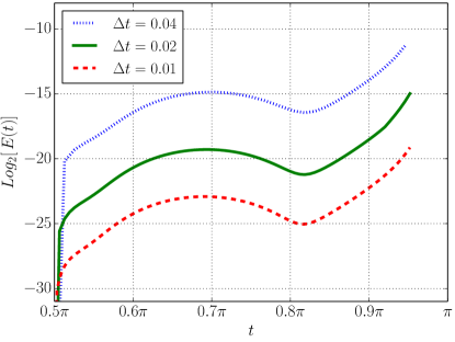
Figure 4: Convergence test, $c_{3}=0.2$.

Next, we replace the non-adaptive 4th-order Runge-Kutta scheme by the adaptive RKF method. In Fig. 6 and Fig. 6 we show the numerical evolutions of the geometric quantities $\psi$ and $\omega$ for $c_{3}=0.2$.

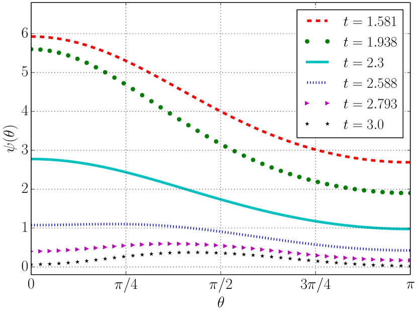
Figure 5: Norm of the Killing vector, $c_{3}=0.2$.

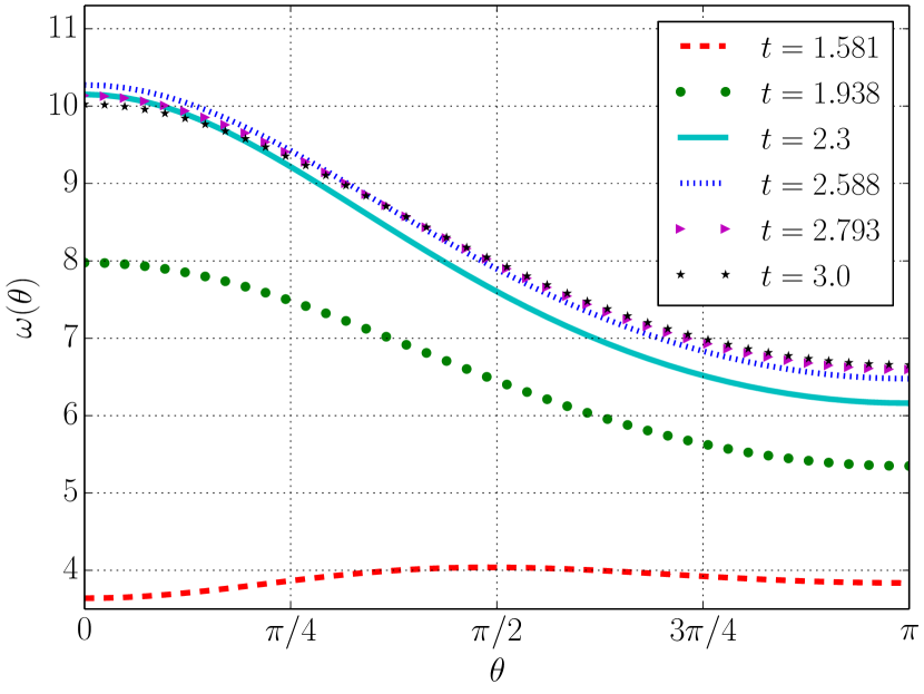
Figure 6: Twist of the Killing vector, $c_{3}=0.2$.

The numerical error in these calculations are shown in Fig. 8 for different values of $c_{3}$. The error tolerance Tol of the RKF method is chosen to be $10^{-8}$. This figure suggests that the numerical errors here remain bounded for a long time. The larger $c_{3}$ is, however, and hence the more inhomogeneous the solution is, the more rapidly the numerical errors grow close to $t=\pi$ as expected. Fig. 8 indicates that the behavior close to $t=\pi$ cannot be improved by decreasing the value of Tol. This suggests that close to $t=\pi$ the numerical errors are not dominated anymore by the time discretization error, but that one of the other error sources discussed in Section 5.3 takes over.

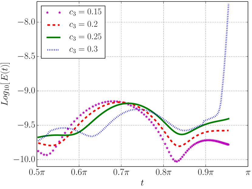
Figure 7: Error propagation for various values of $c_{3}$ and Tol = $10^{-8}$.

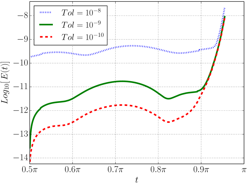
Figure 8: Error propagation for various values of $Tol$ and $c_{3}=0.3$.

Our experience suggests that in fact both the oversampling error and the constraint violation error are significant at late times, in particular, for larger values of $c_{3}$. As a consequence of Eqs. (5.12) – (5.2), the required band limits for the metric components and their time derivatives are small, but the required band limits to resolve $\psi_{0}$, $\omega_{0}$ and their time derivatives are relatively large. This discrepancy, which we associate with the oversampling error, is in fact larger the larger $c_{3}$ is. As already mentioned before, the noise generated by oversampling indeed grows during the evolution.

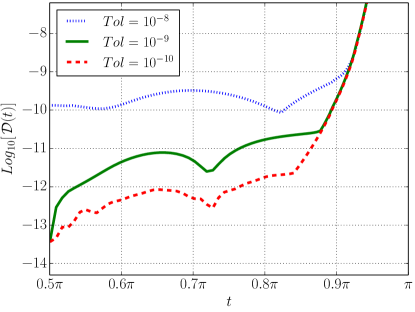
Figure 9: Constraints propagation for various values of Tol and $c_{3}=0.3$.

In order to measure the constraint violation error, we define the quantity

$$\mathcal{D}(t):=\max_{\mu}\>\|\>f_{\mu}(t,\vartheta)-\mathring{\Gamma}_{\mu}(t,\vartheta)\>\|_{L^{2}(\mathbb{S}^{2})}.$$

In Fig. 9, we show the evolution of this quantity for $c_{3}=0.3$. At late times, the curves look very similar to the ones of $E(t)$ in Fig. 8. This suggests that the constraint violation error contributes significantly to the total numerical error.

5.5 Numerical evolutions in wave map gauge

In this section we describe numerical computations for the same spacetimes as before, but using a different coordinate gauge. To this end, we want to choose the same initial data as before, but work with different gauge source functions. Both the gauge constraint Eq. (3.5) and the physical constraints Eq. (3.6) clearly have to be satisfied at the initial time. Since we do not want to resolve these complicated nonlinear PDEs, our strategy is to use exactly the same initial data for the values of the metric components and their first time derivative values, and also exactly the same initial values of the gauge source functions as before. In order to implement a different coordinate gauge, we then apply the following “gauge driver condition” during the evolution whose purpose is to rapidly drive the gauge source functions from their initial values fixed by the gauge constraint towards the target gauge source functions $\hat{f}_{\mu}$:

$$f_{\mu}=(\mathring{\Gamma}_{\mu}|_{t_{0}}-\hat{f}_{\mu})e^{-q(t-t_{0})}+\hat{f}_{\mu}.$$ (5.20)

Here the parameter $q$ controls how rapidly the gauge is driven towards the target. The quantities $\mathring{\Gamma}_{\mu}|_{t_{0}}$ are calculated from the initial data and are understood as functions of the spatial coordinates only. Notice that different gauge drivers for the generalized wave representation of Einstein’s equations were considered in [32]. Eq. (5.20) guarantees that the gauge constraint is satisfied at the initial time. As discussed at the end of Section 3.1, the physical constraints, even though they pose highly non-trivial restrictions on the choice of the initial data because they are essentially linear combinations of the well-known Hamiltonian and momentum constraints, turn out to not be restrictions on the gauge source functions. Hence it is not necessary to introduce terms in Eq. (5.20) which account for the first time derivative of $\mathring{\Gamma}_{\mu}$ at $t=t_{0}$.

We apply this idea to calculate the same spacetimes as before, but now we choose the wave gauge as the target gauge, which is defined by the condition $\hat{f}_{\mu}=0$. For our numerical tests we choose $q=10$ in Eq. (5.20). Before we present our numerical results we notice that it is straightforward to derive the formula

$$t_{(w)}=\dfrac{\pi}{2}+\dfrac{1}{2}\log\left(\dfrac{1-\cos t}{1+\cos t}\right),$$ (5.21)

which for our spacetimes relates the time coordinate $t$ in areal gauge (used in Section 5.4) and the time coordinate $t_{(w)}$ in wave map gauge. This formula holds identically even though Eq. (5.20) is strictly speaking not the exact wave map gauge. However as a consequence of $\mathring{\Gamma}_{0}|_{t_{0}=\pi/2}=0$ which follows from Eq. (5.10), the target gauge source function $\hat{f}_{0}=0$ agrees identically with $f_{0}=0$. Eq. (5.21) is then obtained by solving the exactly homogeneous wave map equation for the wave map time coordinate function with appropriate initial conditions. Eq. (5.21) allows us to make direct comparisons between our results here and the results in the previous section. In particular, it reveals that the wave time slices $t_{(w)}=const$ are the same as the areal time slices $t=const$ (for different constants), and, the “singularities” at $t=0,\pi$ are shifted to infinity, in particular, $t_{(w)}\to\infty$ for $t\to\pi$. We point out however that it is not possible to derive a formula which relates the spatial coordinates in both gauges. This is true even if $q$ in Eq. (5.20) was so large that we could consider our gauge as the exact wave map gauge. This is a consequence of the fact that the homogeneity of the wave equations for the spatial wave map coordinates is destroyed by terms given by the reference metric Eq. (3.9). In fact we shall demonstrate below that the spatial coordinates on each time slice are different in areal and wave map coordinates.

In order to obtain a more geometric and detailed comparison of the two gauges, we consider the Eikonal equation following [19]

$$\nabla_{a}\tau\nabla^{a}\tau=-1.$$ (5.22)

Let $\tau$ be a smooth solution of the initial value problem of the Eikonal equation with smooth initial data $\tau_{0}:\Sigma_{0}\rightarrow\mathbb{R}$ prescribed freely on any smooth Cauchy surface $\Sigma_{0}$ in any smooth globally hyperbolic spacetime. The method of characteristics applied to this PDE allows to prove that such a solution indeed always exists at least sufficiently close to the initial hypersurface $\Sigma_{0}$. For definiteness now we restrict to the case of zero initial data $\tau_{0}=0$ for all of what follows. Fix any point $p$ in the timelike future of $\Sigma_{0}$ in the spacetime and consider any timelike geodesic through $p$ (with unit tangent vector). Any such geodesic must intersect $\Sigma_{0}$ at some point $x_{0}$ in the past of $p$. There is precisely one such timelike geodesic through $p$ with unit tangent vector which intersects $\Sigma_{0}$ perpendicularly in $x_{0}$ and hence the point $x_{0}$ is uniquely determined. The value $\tau(p)$ of the solution $\tau$ of the Eikonal equation with zero initial data then represents the proper time along this timelike geodesic from $x_{0}$ to $p$. The quantity $\tau$ is therefore a meaningful geometric scalar quantity which can be used to compare our numerical spacetimes, in particular when the same spacetime is calculated in different coordinate gauges. We proceed as follows. For initial data parameters $R_{0}=2$, $c_{1}=1$ and $c_{3}=0.1$ (see Section 5.2):

1. We calculate the corresponding solution of Einstein’s evolution equations in areal gauge (in the same way as in Section 5.4) and of the Eikonal equation Eq. (5.22) (with zero initial data) up to $t=3$. The value of the resulting $\tau$ function on the $t=3$-surface expressed with respect to spatial areal coordinates yields the dashed curve in Fig. 11.

2. Eq. (5.21) implies that $t=3$ corresponds to $t_{(w)}\approx 4.217$. For the same initial data parameters as in the first step, we calculate the corresponding solution of Einstein’s evolution equations in wave gauge numerically (using the gauge driver condition Eq. (5.20) with $q=10$) and of the Eikonal equation Eq. (5.22) (with zero initial data) up to $t_{(w)}\approx 4.217$. The value of the resulting $\tau$ function on the $t_{(w)}\approx 4.217$-surface expressed with respect to spatial wave map coordinates yields the continuous curve in Fig. 11.

Since the $t=3$-surface and the $t_{(w)}\approx 4.217$-surface represent the same geometric surface in our spacetime and since $\tau$ is a geometric scalar quantity, the value of the solution of the Eikonal equation on this surface should be the same function in both steps above. However, since this function is expressed in terms of different spatial coordinates, namely areal coordinates in the first step and wave map coordinates in the second step, the two curves in Fig. 11 are slightly different. Hence Fig. 11 can be understood as a representation of the difference of these two sets of spatial coordinates. This difference is emphasized in Fig. 11 where the two curves in Fig. 11 are subtracted directly. Intuitively, these two sets of spatial coordinates should agree at geometrically distinct points, namely, at the poles and also at the equator as a consequence of a reflection symmetry which is inherent to our particular class of exact solutions. Indeed the difference curve in Fig. 11 is zero at the poles $\theta=0,\pi$ and the equator $\theta=\pi/2$.

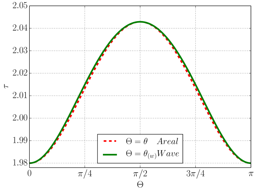
Figure 10: Proper time comparison.

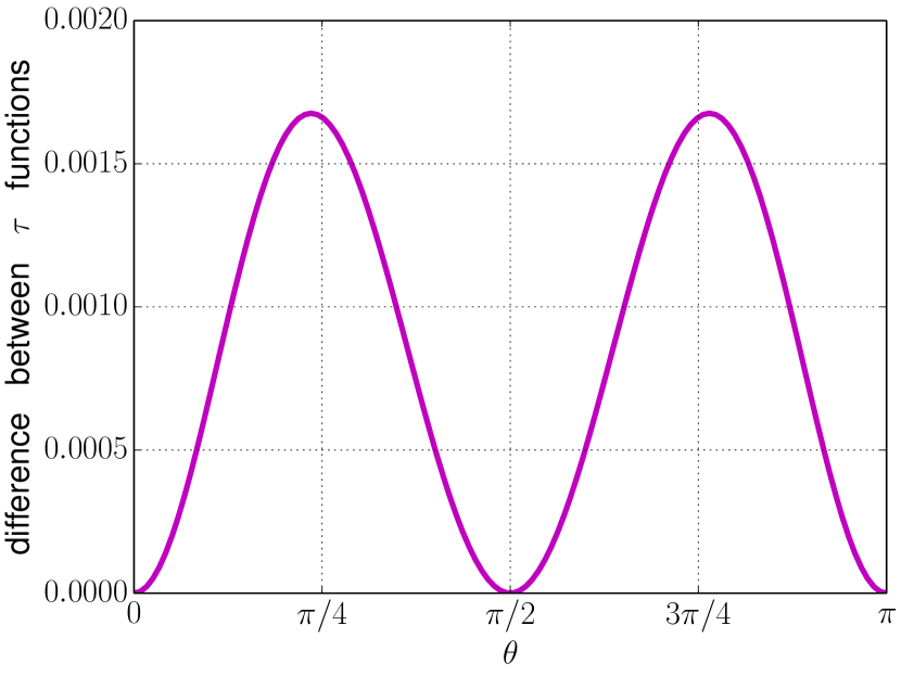
Figure 11: Difference of the proper times.

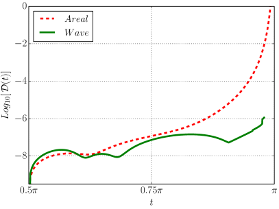
Figure 12: Comparison of the constraint violations.

Next, we present plots of the constraint violations in both gauges; see Fig. 12. The dashed curve has been calculated in areal gauge (in the first step above). The continuous curve has been calculated in wave map gauge (in the second step above), but has then been expressed in terms of the areal time function by means of Eq. (5.21). It is interesting to notice that the constraint violations are significantly smaller in wave map gauge than they are in areal gauge towards the end of the numerical evolution.

Finally we comment on the fact that in wave map gauge the shift quantity $\beta$ in Eq. (3.7) is a non-trivial non-zero function in contrast to areal gauge; see Eq. (5.7). When $\beta$ cannot be assumed to be zero identically, the algebraic complexity of the evolution equations is increased dramatically. It is surprising that irrespective of this it appears that we get better numerical results in wave map than in areal gauge.

6 Discussion

The purpose of our work here was to introduce a numerical approach to solve the Cauchy problem for spacetimes which involve the manifold $\mathbb{S}^{2}$. We employ a fully regular representation of the Einstein equations based on the spin-weighted spherical transform and the generalized wave map formalism. This allows us to account for all singular terms explicitly which usually arise as a consequence of the coordinate singularities of polar coordinates at the poles of the $2$-sphere. Our numerical infrastructure is based on the spin-weight formalism and corresponding transforms introduced in [4, 3]. We have extended this infrastructure so that it now provides an efficient treatment of axially symmetric functions on the $2$-sphere, reducing the complexity $\mathcal{O}(L^{3})$ of the full transform to the complexity $\mathcal{O}(L^{2})$. We therefore expect this method to be useful also for other applications in future work. We have also demonstrated the consistency and feasibility of our approach by means of numerical studies of certain inhomogeneous cosmological solutions of the Einstein’s equations.

As another application of this method we are currently studying the critical behavior of perturbations of the Nariai spacetime [4, 3]. In particular it is suggested that larger amplitudes of the perturbations, which had not been studied before, could lead to the formation of cosmological black holes. It would be of great interest to explore the threshold solutions and the expected cosmological black hole solutions as well as consequences for the longstanding cosmic no-hair and cosmic censorship conjectures. Other conceivable interesting applications where our numerical infrastructure can be applied directly are Robinson-Trautman solutions [15] and Ricci flow [35].

Appendix A The generalized wave map formalism

Whether we want to solve the Cauchy problem for the $3+1$-Einstein vacuum equations $G_{ab}+\Lambda g_{ab}=0$ or for the $2+1$ equations (2.1), the first task is always to extract hyperbolic evolution equations and constraint equations with well-understood propagation properties from the equation for the Ricci tensor of the unknown metric. We shall now briefly discuss the “generalized wave map formalism”. In most of the literature, the related (but not covariant) generalized wave/harmonic formalism is used. While this is sufficient for many applications, it is a drawback for us. In fact, for applications with spatial $\mathbb{S}^{2}$-topologies covered by a single singular polar coordinate system, it is far more convenient to work with actual covariant quantities (i.e., smooth tensor fields). The reason is that frame components of smooth tensor fields on $\mathbb{S}^{2}$ have well-defined spin-weights (despite of the fact that the frame itself is singular at the poles) so that they are expandable in spin-weighted spherical harmonics, which are globally defined regular ‘functions’ on the $2$-sphere (even though their coordinate representation may be singular). It turns out that expressing everything with respect to these bases, renders the equations manifestly regular.

To this end, we discuss the geometric formulation of the wave map gauge [21]. We consider a map $\Phi:M\to\bar{M}$ between two general smooth 4-dimensional manifolds $M$ and $\bar{M}$ (or open subsets thereof) equipped with Lorentzian metrics $h_{ab}$ and $\bar{h}_{ab}$. The map $\Phi$ is called a wave map if it extremizes the functional

$$\mathcal{F}[\Phi]=\int_{M}\mathrm{tr}_{h}(\Phi^{*}\bar{h})\,\mathrm{Vol}_{h}.$$

In coordinate charts $(x^{\mu})$ on $M$ and $(y^{\alpha})$ on $\bar{M}$ we obtain the Euler-Lagrange equations for the coordinate representation $y^{\alpha}=y^{\alpha}(x^{\mu})$ of $\Phi$

$$\Box_{h}y^{\alpha}+\bar{\Gamma}^{\alpha}{}_{\beta\gamma}h^{\mu\nu}\frac{\partial y^{\beta}}{\partial x^{\mu}}\frac{\partial y^{\gamma}}{\partial x^{\nu}}=0.$$ (A.1)

Here, $\bar{\Gamma}^{\alpha}{}_{\beta\gamma}$ are the Christoffel symbols for the metric $\bar{h}_{ab}$ in the coordinate basis on $\bar{M}$, and $\Box_{h}$ is the wave operator for scalar functions defined by $h_{ab}$. This equation is called the wave-map equation. More details can be found in [12]. If the manifolds were Riemannian then the analogous equation would characterize a harmonic map between $M$ and $\bar{M}$. Let us point out that the left hand side of the equation defines a geometric object, namely a section in the pull-back bundle $\Phi^{*}T\bar{M}$. This is not immediately obvious due to the appearance of the Christoffel symbols in the second term. However, the tensorial character of that term under change of coordinates in $\bar{M}$ is compensated for by the first term which, by itself, is also non-tensorial under such coordinate transformations.

The generalized wave-map equation is the equation (A.1) with a non-vanishing, arbitrary right hand side, a section in $\Phi^{*}T\bar{M}$ with coordinate representation $f^{\alpha}$

$$\Box_{h}y^{\alpha}+\bar{\Gamma}^{\alpha}{}_{\beta\gamma}h^{\mu\nu}\frac{\partial y^{\beta}}{\partial x^{\mu}}\frac{\partial y^{\gamma}}{\partial x^{\nu}}=-f^{\alpha}.$$ (A.2)

The minus sign on the right-hand side is a matter of conventions. Suppose now that $\bar{M}=M$ and $\Phi=id_{M}$. Then $(x^{\mu})$ and $(y^{\alpha})$ are two coordinate charts for $M$ and (A.2) can be read as an equation determining the coordinate system $(y^{\alpha})$ for $M$ by imposing a geometrical gauge condition. This equation is a semi-linear wave equation of $M$ which has solutions near any Cauchy surface so that such a coordinate gauge always exists locally.

Choosing the coordinates according to this gauge, i.e., putting $x^{\mu}=y^{\mu}$ and expressing the wave operator in these coordinates yields the equation

$$(-\Gamma^{\alpha}{}_{\beta\gamma}+\bar{\Gamma}^{\alpha}{}_{\beta\gamma})h^{\beta\gamma}=-f^{\alpha},$$

where $\Gamma^{\alpha}{}_{\beta\gamma}$ are the Christoffel symbols of the metric $h$ on $M$. In this equation the tensorial character becomes manifest since the left hand side involves the difference of two connection coefficients so it gives the components of a vector field in the coordinate basis of the $(x^{\mu})$. Therefore, this equation holds in any basis on $M$ as long as we interpret the Christoffel symbols as the connection coefficients with respect to the chosen basis. Note also that this implies that imposing the equation (A.2) does not constitute a condition on the coordinate system $(x^{\alpha})$ but a condition on the metric components in their dependence on the coordinates. We define the vector field $\mathcal{D}^{a}$ in terms of its components

$$\mathcal{D}^{\alpha}:=(-\Gamma^{\alpha}{}_{\beta\gamma}+\bar{\Gamma}^{\alpha}{}_{\beta\gamma})h^{\beta\gamma}+f^{\alpha}.$$ (A.3)

So, $\mathcal{D}^{a}=0$ when (A.2) is imposed. A metric $h_{ab}$ which is restricted by $\mathcal{D}^{a}=0$ is said to be in wave map gauge (with respect to $\bar{h}_{ab}$); in Eq. (3.9) we fix a particular metric $\bar{h}_{ab}$. We point out that the wave map gauge reduces to the widely used generalized wave/harmonic gauge characterized by $\Box x^{\mu}=-f^{\mu}$ on space-times with topology $\mathbb{R}^{4}$ when the Minkowski metric in Cartesian coordinates $x^{\mu}$ is used as a reference metric $\bar{h}_{ab}$.

References

- [1] E. Ames, F. Beyer, J. Isenberg, and P. G. LeFloch. Quasilinear Hyperbolic Fuchsian Systems and AVTD Behavior in -Symmetric Vacuum Spacetimes. Ann. Henri Poincaré, 14(6):1445–1523, 2013.
- [2] F. Beyer. A spectral solver for evolution problems with spatial -topology. J. Comp. Phys., 228(17):6496–6513, 2009.
- [3] F. Beyer, B. Daszuta, and J. Frauendiener. A spectral method for half-integer spin fields based on spin-weighted spherical harmonics. Class. Quantum Grav., 32(17):175013, 2015.
- [4] F. Beyer, B. Daszuta, J. Frauendiener, and B. Whale. Numerical evolutions of fields on the 2-sphere using a spectral method based on spin-weighted spherical harmonics. Class. Quantum Grav., 31(7):075019, 2014.
- [5] F. Beyer and L. Escobar. Graceful exit from inflation for minimally coupled Bianchi A scalar field models. Class. Quantum Grav., 30(19):195020, 2013.
- [6] F. Beyer and J. Hennig. Smooth Gowdy-symmetric generalized Taub–NUT solutions. Class. Quantum Grav., 29(24):245017, 2012.
- [7] F. Beyer and J. Hennig. An exact smooth Gowdy-symmetric generalized Taub–NUT solution. Class. Quantum Grav., 31(9):095010, 2014.
- [8] M. Boyle, L. Lindblom, H. P. Pfeiffer, M. A. Scheel, and L. E. Kidder. Testing the accuracy and stability of spectral methods in numerical relativity. Phys. Rev. D, 75(2):024006, 2007.
- [9] O. Brodbeck, S. Frittelli, P. Hübner, and O. A. Reula. Einstein’s equations with asymptotically stable constraint propagation. J. Math. Phys., 40(2):909, 1999.
- [10] B. Brügmann. A pseudospectral matrix method for time-dependent tensor fields on a spherical shell. J. Comp. Phys., 235:216–240, 2013.
- [11] M. W. Choptuik, E. W. Hirschmann, S. L. Liebling, and F. Pretorius. An axisymmetric gravitational collapse code. Class. Quantum Grav., 20(9):1857, 2003.
- [12] Y. Choquet-Bruhat. General Relativity and the Einstein Equations. Oxford mathematical monographs. Oxford University Press, Oxford, New York, 2008.
- [13] Y. Choquet-Bruhat and R. P. Geroch. Global aspects of the Cauchy problem in general relativity. Commun. Math. Phys., 14(4):329–335, 1969.
- [14] P. T. Chruściel. On space-times with symmetric compact Cauchy surfaces. Ann. Phys., 202(1):100–150, 1990.
- [15] H. P. de Oliveira, E. L. Rodrigues, and J. E. F. Skea. Numerical evolution of general Robinson-Trautman spacetimes: Code tests, wave forms, and the efficiency of the gravitational wave extraction. Phys. Rev. D, 84(4):044007, 2011.
- [16] D. R. Durran. Numerical Methods for Fluid Dynamics, volume 32 of Texts in Applied Mathematics. Springer, New York, NY, 2010.
- [17] B. Fornberg. A Practical Guide to Pseudospectral Methods. Cambridge University Press, 1998.
- [18] Y. Fourès-Bruhat. Théorème d’existence pour certains systèmes d’équations aux dérivées partielles non linéaires. Acta Mathematica, 88(1):141–225, 1952.
- [19] J. Frauendiener. Numerical treatment of the hyperboloidal initial value problem for the vacuum Einstein equations. II. The evolution equations. Phys. Rev. D, 58(6):064003, 1998.
- [20] J. Frauendiener and T. Vogel. Algebraic stability analysis of constraint propagation. Class. Quantum Grav., 22(9):1769–1793, 2005.
- [21] H. Friedrich. On the global existence and the asymptotic behavior of solutions to the Einstein-Maxwell-Yang-Mills equations. J. Diff. Geom., 34:275–345, 1991.
- [22] D. Garfinkle. Numerical simulations of Gowdy spacetimes on . Phys. Rev. D, 60(10):104010, 1999.
- [23] D. Garfinkle. Harmonic coordinate method for simulating generic singularities. Phys. Rev. D, 65(4):044029, 2002.
- [24] R. P. Geroch. A Method for Generating Solutions of Einstein’s Equations. J. Math. Phys., 12(6):918, 1971.
- [25] R. Gómez, L. Lehner, P. Papadopoulos, and J. Winicour. The eth formalism in numerical relativity. Class. Quantum Grav., 14(4):977–990, 1997.
- [26] C. Gundlach, J. Martín-García, G. Calabrese, and I. Hinder. Constraint damping in the Z4 formulation and harmonic gauge. Class. Quantum Grav., 22(17):3767–3774, 2005.
- [27] J. Hennig. Fully pseudospectral time evolution and its application to dimensional physical problems. J. Comp. Phys., 235:322–333, 2013.
- [28] M. Holst, L. Lindblom, R. Owen, H. P. Pfeiffer, M. A. Scheel, and L. E. Kidder. Optimal constraint projection for hyperbolic evolution systems. Phys. Rev. D, 70(8):084017, 2004.
- [29] K. M. Huffenberger and B. D. Wandelt. Fast and Exact Spin-s Spherical Harmonic Transforms. Astro. J. Suppl. Series, 189(2):255–260, 2010.
- [30] L. Lehner, O. A. Reula, and M. Tiglio. Multi-block simulations in general relativity: high-order discretizations, numerical stability and applications. Class. Quantum Grav., 22(24):5283–5321, 2005.
- [31] L. Lindblom, M. A. Scheel, L. E. Kidder, H. P. Pfeiffer, D. Shoemaker, and S. A. Teukolsky. Controlling the growth of constraints in hyperbolic evolution systems. Phys. Rev. D, 69(12):124025, 2004.
- [32] L. Lindblom and B. Szilagyi. Improved gauge driver for the generalized harmonic Einstein system. Phys. Rev. D, 80(8):084019, 2009.
- [33] V. Moncrief. The space of (generalized) Taub-Nut spacetimes. J. Geom. Phys., 1(1):107–130, 1984.
- [34] V. Moncrief. Reduction of Einstein’s equations for vacuum space-times with spacelike isometry groups. Ann. Phys., 167(1):118–142, 1986.
- [35] J. Morgan and T. Gang. Ricci Flow and the Poincaré Conjecture. Clay Mathematics Monographs, 2007.
- [36] E. T. Newman and R. Penrose. Note on the Bondi-Metzner-Sachs Group. J. Math. Phys., 7(5):863, 1966.
- [37] E. T. Newman, L. Tamburino, and T. Unti. Empty-Space Generalization of the Schwarzschild Metric. J. Math. Phys., 4(7):915, 1963.
- [38] F. Pretorius. Evolution of Binary Black-Hole Spacetimes. Phys. Rev. Lett., 95:121101, 2005.
- [39] H. Ringström. The Cauchy Problem in General Relativity. ESI Lectures in Mathematics and Physics. European Mathematical Society, Zürich, Switzerland, 2009.
- [40] O. Rinne. An axisymmetric evolution code for the Einstein equations on hyperboloidal slices. Class. Quantum Grav., 27(3):035014, 2010.
- [41] T. Risbo. Fourier transform summation of Legendre series and D-functions. J. Geodesy, 70(7):383–396, 1996.
- [42] H. Stephani, D. Kramer, M. A. H. MacCallum, C. Hoenselaers, and E. Herlt. Exact solutions of Einstein’s field equations. Cambridge University Press, second edition, 2003.
- [43] M. Sugiura. Unitary Representations and Harmonic Analysis. An Introduction. North Holland, 1990.
- [44] A. H. Taub. Empty Space-Times Admitting a Three Parameter Group of Motions. Ann. Math., 53(3):472–490, 1951.
- [45] S. Trapani and J. Navaza. Calculation of spherical harmonics and Wigner d-functions by FFT. Applications to fast rotational matching in molecular replacement and implementation into AMoRe. Acta Cryst. A, 62(4):262–269, 2006.
- [46] A. Vretblad. Fourier Analysis and Its Applications. Springer New York, 2003.