A Circular Interference Model for
Asymmetric Aggregate Interference

Abstract

Scaling up the number of base stations per unit area is one of the major trends in mobile cellular systems of the fourth (4G)- and fifth generation (5G), making it increasingly difficult to characterize aggregate interference statistics with system models of low complexity. This paper proposes a new circular interference model that aggregates given interferer deployments to power profiles along circles. The model accurately preserves the original interference statistics while considerably reducing the amount of relevant interferers. In comparison to common approaches from stochastic geometry, it enables to characterize cell-center- and cell-edge users, and preserves effects that are otherwise concealed by spatial averaging. To enhance the analysis of given power profiles and to validate the accuracy of the circular model, a new finite sum representation for the sum of Gamma random variables with integer-valued shape parameter is introduced. The approach allows to decompose the distribution of the aggregate interference into the contributions of the individual interferers. Such knowledge is particularly expedient for the application of base station coordination- and cooperation schemes. Moreover, the proposed approach enables to accurately predict the corresponding signal-to-interference-ratio- and rate statistics.

I Introduction and Contributions

In mobile cellular systems of the fourth (4G)- and fifth generation (5G), the number of Base Stations per unit area is expected to grow substantially [15]. One of the main performance limiting factors in such dense networks is aggregate interference. Hence, its accurate statistical characterization becomes imperative for network design and analysis. Although abstraction models such as the Wyner model and the hexagonal grid have been reported two [51]- or even five decades ago [24], mathematically tractable interference statistics are still the exception rather than the rule. Moreover, the emerging network topologies fundamentally challenge various time-honored aspects of traditional network modeling [26].

In current literature, BS deployment models mainly follow the trend away from being fully deterministic towards complete spatial randomness [4, 45]. However, even the new approaches only yield known expression for the Probability Density Function (PDF) of the aggregate interference, if particular combinations of spatial node distributions, path loss models and user locations are given [22]. For example, a finite, typically small number of interferers together with certain fading distributions, such as Rayleigh, lognormal or Gamma allows to exploit literature on the sum of Random Variables  [3, 9, 10, 46, 7, 34, 23, 35, 53, 52, 47, 38, 33, 44, 8, 19, 5, 11, 29, 39].

Otherwise, tractable interference statistics have mainly been reported in the field of stochastic geometry. This powerful mathematical framework recently gained momentum as the only available tool that provides a rigorous approach to modeling, analysis and design of networks with a substantial amount of nodes per unit area [18, 16, 14, 30, 50, 12, 13, 6, 43, 25, 21, 27, 28, 49, 17]. However, when closed-form expressions are desired, it imposes its own particular limitations, typically including spatial stationarity and isotropy of the scenario [22, 30, 27]. Hence, the potential to consider an asymmetric interference impact is very limited and notions such as cell-center and cell-edge are, in general, not accessible. The contributions of this paper outline as follows:

• A new circular interference model is introduced. The key idea is to map arbitrary out-of-cell interferer deployments onto circles of uniformly spaced nodes such that the original aggregate interference statistics can accurately be reproduced. The model greatly reduces complexity as the number of participating interferers is significantly reduced.

• A mapping scheme that specifies a procedure for determining the power profiles of arbitrary interferer deployments is proposed. Its performance is evaluated by means of Kolmogorov-Smirnov statistics. The test scenarios are modeled by Poisson Point Processes so as to confront the regular circular structure with complete spatial randomness. It is shown that the individual spatial realizations exhibit largely diverging power profiles.

• A new finite sum representation for the PDF of the sum of Gamma RVs with integer-valued shape parameter is introduced to further enhance and validate interference analysis with the circular model. Its restriction to integer-valued shape parameters is driven by relevant use cases for wireless communication engineering and the availability of exact solutions. The key strength of the proposed approach lies in the ability to decompose the interference distribution into the contributions of the individual interferers.

• Statistics of aggregate interference with asymmetric interference impact are investigated. The asymmetry is induced by eccentrically placing a user in a generic, isotropic scenario. This setup is achieved by applying the introduced circular model with uniform power profiles. On top of that, the model enables to employ the proposed finite sum representation. It is shown that the partition of the interference distribution is particularly useful to identify candidate BSs for user-centric BS collaboration schemes. Moreover, the framework allows to predict the corresponding Signal-to-Interference Ratio (SIR)- and rate statistics.

This paper is organized as follows. sections II and III introduce the circular interference model and the new finite sum representation for the sum of Gamma RVs with integer-valued shape parameter, respectively. section IV presents a mapping scheme and validates the applicability of the circular model. section V investigates aggregate interference statistics and the performance of BS collaboration schemes at eccentric user locations. section VI concludes the work. The main focus of this paper is on downlink transmission in cellular networks. A comparable framework for the uplink is found in [48].

II Circular Interference Model

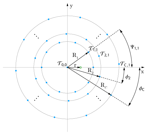
Figure 1: Circular interference model with $C$ circles of radius $R_{c}$ and phase $\phi_{c}$, $c\in\{1,\ldots,C\}$, and user at $(r,0)$. $\mathcal{T}_{c,n}$ denotes the nodes of the model.

Consider the serving BS to be located at the origin. The proposed circular interference model is composed of $C$ concentric circles of interferers, as shown in fig. 1. On circle $c\in\{1,\ldots,C\}$ of radius $R_{c}$, $N_{c}$ interfering nodes are spread out equidistantly. The interferer locations are expressed in terms of polar coordinates as $(R_{c},\Psi_{c,n})$, where $\Psi_{c,n}=2\pi n/N_{c}-\phi_{c}$, with $n\in\{1,\ldots,N_{c}\}$ and $\phi_{c}\in[0,2\pi)$. Each node is unambiguously assigned to a tuple $(c,n)$ and labeled as $\mathcal{T}_{c,n}$. The central BS is denoted as $\mathcal{T}_{0,0}$. Some of the interferers on the circles may also become serving nodes when BS collaboration schemes are applied, as will be shown later in section V-C.

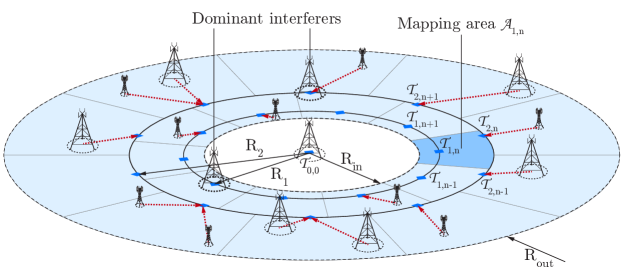
Figure 2: Circular interference model with two circles, i.e., $C=2$. Characteristics of an arbitrary heterogeneous interferer deployment are condensed to circles of equidistantly spaced nodes $\mathcal{T}_{c,n}$ such that the original interference statistics can accurately be reproduced. A mapping scheme is presented in section IV. The original BSs are distributed within an annulus of inner radius $R_{\rm in}$ and outer radius $R_{\rm out}$.

The interferers on the circles do not necessarily represent real physical sources. As illustrated in fig. 2, they rather correspond to the $N_{c}$ mapping points of an angle-dependent power profile $p_{c}[n]$, with $\sum_{n=1}^{N_{c}}p_{c}[n]=1$. Exemplary profiles of a single circle are shown in fig. 3. Intuitively, $p_{c}[n]$ condenses the interferer characteristics of an annulus with inner radius $R_{\rm in}$ and possibly infinite outer radius $R_{\rm out}$ such that the circular model equivalently reproduces the original BS deployment in terms of interference statistics. This technique enables to represent substantially large networks by a finite- and well-defined constellation of nodes. By reducing the number of relevant interferers, it greatly reduces complexity and thus allows to apply finite sum-representations as those introduced in section III.

TABLE I: Parameters of the circular interference model.

Symbol	Annotation
$R_{\rm in}$	Inner radius of mapping region, $R_{\rm in}\geq 0$
$R_{\rm out}$	Outer radius of mapping region, $R_{\rm out}>R_{\rm in}$
$C$	Number of interferer circles, $C\in\mathbb{N}^{+}$
$R_{c}$	Radius of circle $c$, $c\in\{1,\ldots,C\}$, $R_{c}>0$
$\phi_{c}$	Phase of circle $c$, $c\in\{1,\ldots,C\}$ $\phi_{c}\in[-\frac{\pi}{N_{c}},\frac{\pi}{N_{c}}]$
$N_{c}$	Number of mapping points, $c\in\{1,\ldots,C\}$, $N_{c}\in\mathbb{N}^{+}$
$P_{c}$	Total transmit power of circle $c$, $c\in\{1,\ldots,C\}$, $P_{c}>0$
$p_{c}[n]$	Power profile of circle $c$, $c\in\{1,\ldots,C\}$, $n\in\{1,\ldots,N_{c}\}$, $p_{c}[n]\in[0,1]$

table I summarizes the parameters of the model. Typically, the size of the mapping region, as specified by $R_{\rm in}$ and $R_{\rm out}$, is predetermined by the scenario. The freely selectable variables are the amount of circles $C$ and, for each circle, the phase $\phi_{c}$, the radius $R_{c}$ and the number of mapping points $N_{c}$, respectively. section IV presents systematic experiments to provide a reference for the parameter setting and proposes a mapping scheme to determine power profiles $p_{c}[n]$ and transmit powers $P_{c}$, respectively.

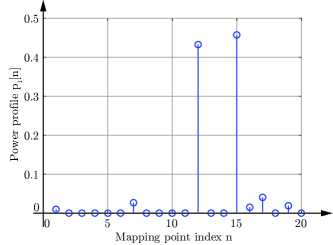
(a) 10 interferers

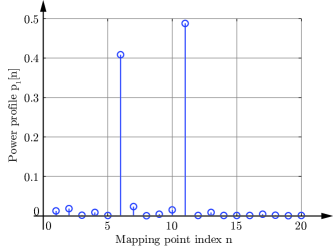
(b) 100 interferers

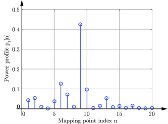
(c) 1 000 interferers

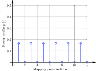
(d) Hexagonal grid

Figure 3: Power profiles of circular models with one circle, i.e, $C=1$, for three stochastic interference scenarios ((a)-(c)) with $N_{1}=20$ mapping points, and for a hexagonal grid with $N_{1}=12$ mapping points, respectively. The stochastic BS distributions are modeled by a PPP of intensity $\lambda=0.01/{\rm Unit\ Area}$. The expected number of interferers as denoted by the figure labels, is varied by altering the scenario size.

A signal from node $\mathcal{T}_{c,n}$, located at $(R_{c},\Psi_{c,n})$, to a user at $(r,0)$ experiences path loss $\ell(d_{c,n}(r))$, where $d_{c,n}(r)=\sqrt{R_{c}^{2}+r^{2}-2R_{c}r\cos(\Psi_{c,n})}$ (conf. fig. 1) and $\ell(\cdot)$ is an arbitrary distance-dependent path loss law, as well as fading, which is modeled by statistically independent RVs $G_{c,n}$. The received power from node $\mathcal{T}_{c,n}$ at position $(r,0)$ is determined as

$$P_{{\rm Rx},c,n}(r)=P_{c}\,p_{c}[n]\,\ell(d_{c,n}(r))\,G_{c,n},$$ (1)

where $P_{c}$ denotes the total transmit power of circle $c$. It is important to note that the term $P_{{\rm Rx},c,n}(r)$ can be interpreted as a RV $G_{c,n}$, which is scaled by a factor of $P_{c}\,p_{c}[n]\,\ell(d_{c,n}(r))$.

The nodes employ omnidirectional antennas with unit antenna gain. Characteristics of antenna directivity are incorporated into the power profile. In general, the central cell will have an irregular shape that can be determined by Voronoi tesselation [31]. For simplicity, the small ball approximation from [31] is applied. A user is considered as cell-edge user, if it is located at the edge of the central Voronoi cell’s inscribing ball. This approximation misses some poorly covered areas at the actual cell-edge with marginal loss of accuracy [31].

Let $\mathcal{S}$ and $\mathcal{I}$ denote the sets of nodes $\mathcal{T}_{c,n}$ corresponding to desired signal and interference, respectively. Then, the aggregate signal- and interference powers are calculated as

$$S(r)=\sum_{\{(c,n)|\mathcal{T}_{c,n}\in\mathcal{S}\}}P_{{\rm Rx},c,n}(r),$$ (2)

$$I(r)=\sum_{\{(c,n)|\mathcal{T}_{c,n}\in\mathcal{I}\}}P_{{\rm Rx},c,n}(r),$$ (3)

with $P_{{\rm Rx},c,n}(r)$ from eq. 1. The set $\mathcal{S}$ may include the central node $\mathcal{T}_{0,0}$ as well as nodes on the circles, if collaboration among the BSs is employed. The incoherence assumption is exploited for a more realistic assessment of the co-channel interference [41]. Following the interpretation of eq. 1, eqs. 2 and 3 can be viewed as sums of scaled RVs, which are supported by a vast amount of literature for certain fading distributions such as Rayleigh, log-normal and Nakagami-m  [3, 9, 10, 46, 7, 34, 23, 35, 53, 52, 47, 38, 33, 44, 8, 19, 5, 11, 29, 39].

The present work places particular focus upon the Gamma distribution due to its wide range of useful features for wireless communication engineering. The next section provides preliminary information and introduces a new theorem on the sum of Gamma RVs. The theorem is introduced before validating the accuracy of the circular model as it is later exploited for this purpose.

III Distribution of the Sum of Gamma Random Variables

III-A Preliminaries

The PDF of a Gamma distributed RV $X$ with shape parameter $k$ and scale parameter $\theta$, i.e., $X\sim\Gamma[k,\theta]$, is defined as

$$f_{X}(x)=\frac{1}{\theta^{k}\Gamma(k)}x^{k-1}e^{-x/\theta},$$ (4)

with $k>0$ and $\theta>0$, respectively. The Gamma distribution exhibits the scaling property, i.e., if $X\sim\Gamma[k,\theta]$, then $aX\sim[k,a\theta]$, $\forall a>0$, as well as the summation property, i.e., if $X_{i}\sim\Gamma[k_{i},\theta]$ with $i=1,2,\ldots,N$, then $\sum_{i=1}^{N}X_{i}\sim\Gamma[\sum_{i=1}^{N}k_{i},\theta]$.

While the latter is convenient to apply, it is the sum of Gamma RVs with distinct scale parameters that has attracted a lot of attention in describing wireless communications though. Most commonly, it emerged in the performance analysis of diversity combining receivers and the study of aggregate co-channel interference under Rayleigh fading [3, 9, 10, 46, 7, 34, 23, 35, 53, 52, 47]. Therefore, communication engineers have considerably pushed the search for closed form statistics.

Representatively, Moschopoulos’ much-cited series expansion in [38] was extended for correlated Gamma RVs in [3]. Other approaches based on the inverse Mellin transform (e.g., [32, 42]) paved the way for representations with a single integral as shown, e.g., in [10] or a Lauricella hypergeometric series as employed, e.g., in [9, 23].

All the aforementioned contributions focus on the sum of Gamma RVs with real-valued shape parameter. The resulting integrals and infinite series, despite being composed of elementary functions, typically yield a slow rate of convergence. Therefore, an accurate approximation by a truncated series requires to keep a high amount of terms and complicates further analysis.

The sum of Gamma RVs with integer shape parameter has mainly been reported in statistical literature. Initial approaches focused on the moment generating function and results were obtained in the form of series expansions [33]. Based on the work of [44], [8] was among the first to formulate a convenient closed form solution. Soon after, the Generalized Integer Gamma (GIG) distribution was published in [19]. This approach was also adopted in wireless communication engineering [46, 34]. In comparison to RVs with real-valued shape parameter, the PDF of the sum of RVs with integer shape parameter allows an exact representation by a finite series.

III-B Proposed Finite Sum Representation

In the analysis of aggregate interference statistics, it is particularly desirable to identify the main distribution-shaping factors, i.e., the interfering sources with the highest impact. However, the expressions in [46] and [34] are not suitable for this task due to multiple nested sums and recursions. The proposed finite-sum representation in this work avoids recursive functions and enables to straightforwardly trace the main determinants of the distribution characteristics.

Theorem III.1.

Let $G_{l}\sim\Gamma[k_{l},\theta_{l}]$ be $L$ independent Gamma RVs with $k_{l}\in\mathbb{N}^{+}$ and all $\theta_{l}$ different. Then, the PDF of $Y=G_{1}+\cdots+G_{L}$ can be expressed as

$$f_{Y}(y)=\sum_{l=1}^{L}\frac{\Lambda_{l}}{\theta_{l}^{k_{l}}}h_{k_{l}-1,l}(0)e^{-y/\theta_{l}}$$ (5)

with

$$\Lambda_{l}=\frac{(-1)^{k_{l}+1}}{(k_{l}-1)!}\prod_{i=1,i\neq l}^{L}\left(1-\frac{\theta_{i}}{\theta_{l}}\right)^{-k_{i}}, \qquad l=1,\ldots,L$$ (6)

$$h_{\delta+1,l}(\zeta)=h_{1,l}(\zeta)h_{\delta,l}(\zeta)+\frac{d}{d\zeta}h_{\delta,l}(\zeta), \qquad\delta=0,\ldots,k_{l}-1$$ (7)

and

$$h_{1,l}(0)=-y+\sum_{i=1,i\neq l}^{L}k_{i}\left(\frac{1}{\theta_{i}}-\frac{1}{\theta_{l}}\right)^{-1}, \qquad l=1,\ldots,L$$ (8)

$$h_{1,l}^{(m)}(0)=m!\sum_{i=1,i\neq l}^{L}k_{i}\left(\frac{1}{\theta_{i}}-\frac{1}{\theta_{l}}\right)^{-m-1}, \qquad m=1,\ldots,k_{l}-1$$ (9)

Proof.

The proof is provided in section -A. ∎

Superscript $(m)$ of $h_{1,l}^{(m)}(\zeta)$ denotes the $m$-th derivative of $h_{1,l}(\zeta)$. The recursive determination of $h_{\delta,l}(\zeta)$ in eq. 7 seemingly interrupts the straightforward calculation of $f_{Y}(y)$. However, $h_{\delta,l}(\zeta)$ is a function of only $h_{1,l}(\zeta)$ and its higher order derivatives. Therefore, the function series in eq. 7 can be evaluated in advance up to the highest required degree $\delta_{\max}=\max_{l}k_{l}-1$.

Thus, the proposed approach enables the exact calculation of $f_{Y}(y)$ in a component-wise manner . In the next step, it is shown how to apply Theorem III.1 in the proposed circular model.

III-C Application in Circular Interference Model

Assume that $G_{c,n}\sim\Gamma[k_{c,n},\theta_{c,n}]$ in eq. 1, with $k_{c,n}\in\mathbb{N}^{+}$ and $\theta_{c,n}>0$. Then, eqs. 2 and 3 represent sums of scaled Gamma RVs $P_{{\rm Rx},c,n}(r)\sim\Gamma[k_{c,n},\theta_{c,n}^{\prime}(r)]$, where $\theta_{c,n}^{\prime}(r)=P_{c}\,p_{c}[n]\,\ell(d_{c,n}(r))\,\theta_{c,n}$. Therefore, their PDFs can be determined by applying Theorem III.1.

The theorem requires all scale parameters to be different. Thus, let $\boldsymbol{\theta}_{\mathcal{I}}(r)$ denote the vector of unique scale parameters $\theta_{c,n}^{\prime}(r)$ with $(c,n)$ from the set $\{(c,n)|\mathcal{T}_{c,n}\in\mathcal{I}\}$. A second vector $\mathbf{k}_{\mathcal{I}}$ contains the corresponding shape parameters. By virtue of the summation property, if $\theta_{c,n}^{\prime}(r)$ occurs multiple times in the set, the respective shape parameter in $\mathbf{k}_{\mathcal{I}}$ is calculated as the sum of shape parameters $k_{c,n}$ of the according entries. The vectors $\boldsymbol{\theta}_{\mathcal{S}}(r)$ and $\mathbf{k}_{\mathcal{S}}$ are obtained equivalently. Then, the PDFs of $S(r)$ and $I(r)$ are expressed as

$$f_{S}(\gamma;r) =\sum_{l=1}^{L_{\mathcal{S}}}\frac{\Lambda_{l}}{\theta_{l}(r)^{k_{l}}}h_{k_{l}-1,l}(0)e^{-\gamma/\theta_{l}(r)},$$ (10)

$$f_{I}(\gamma;r) =\sum_{l=1}^{L_{\mathcal{I}}}\frac{\Lambda_{l}}{\theta_{l}(r)^{k_{l}}}h_{k_{l}-1,l}(0)e^{-\gamma/\theta_{l}(r)},$$ (11)

with $\Lambda_{l}$ and $h_{\delta,l}(\cdot)$ as defined in eqs. 6 and 7. Subscript $l$ indicates the $l$-th components of the vectors $\mathbf{k}_{\mathcal{S}}$ ($\boldsymbol{\theta}_{\mathcal{S}}(r)$) and $\mathbf{k}_{\mathcal{I}}$ ($\boldsymbol{\theta}_{\mathcal{I}}(r)$) and $L_{\mathcal{S}}$ and $L_{\mathcal{I}}$ are their corresponding lengths, respectively.

Hence, employing Theorem III.1 allows to evaluate the exact distributions of the aggregate signal- and interference from the circular model by finite sums. In the following section, this fact is exploited to verify the accuracy of the model.

IV Mapping Scheme for Stochastic Network Deployments

This section presents a procedure to determine the power profiles $p_{c}[n]$ and the corresponding powers $P_{c}$ of the circular model for completely random interferer distributions. Then, systematic experiments are carried out to provide a reference for selecting the free variables $C$ and $N_{c}$, respectively. The parameters $R_{c}$ and $\phi_{c}$ are also specified by the procedure. The accuracy of the approximation is measured by means of the Kolmogorov-Smirnov distance. It is defined as

$$D(r)={\rm sup}_{x}\left|F_{I,{\rm original}}(x;r)-F_{I,{\rm circular}}(x;r)\right|,$$ (12)

where $r$ refers to the user’s eccentricity and $F_{I,{\rm original}}(x;r)$ and $F_{I,{\rm circular}}(x;r)$ denote the aggregate-interference Cumulative Distribution Functions of the original deployment and the circular model, respectively. The corresponding PDFs are obtained by Theorem III.1.

IV-A Mapping Procedure

Data: number of circles $C$; nodes per circle $N_{c}$;

          original base station deployment $\mathcal{N}$;

          inner- and outer radius of mapping region $\mathcal{A}$: $R_{\rm in}$ and $R_{\rm out}$;

Result: $P_{c}$, $p_{c}[n]$, $R_{c}$ and $\phi_{c}$ for all $c\leq C$;

for $c=1\ {\rm to}\ C$ do

       determine $R_{c}$ and $\phi_{c}$ based on the strongest interferer that has not yet been mapped;

      

end for

for $c=1\ {\rm to}\ C$ do

       specify mapping region $\mathcal{A}_{c}$ with inner radius $R_{c}$ and outer radius $R_{c+1}$;

       if $c=1$ then set inner radius of $\mathcal{A}_{c}$ to $R_{\rm in}$; end

       if $c=C$ then set outer radius of $\mathcal{A}_{c}$ to $R_{\rm out}$; end

       compute $P_{c}$ and $p_{c}[n]$ for $\mathcal{A}_{c}$;

      

end for

Algorithm 1 Mapping procedure for circular model.

Let $\mathcal{N}$ denote a (possibly heterogeneous) set of BSs that are arbitrarily distributed within an annulus $\mathcal{A}$ of inner radius $R_{\rm in}$ and outer radius $R_{\rm out}$, as shown in fig. 2. Radius $R_{\rm out}$ as well as the number of nodes in $\mathcal{N}$ could be substantially large. Given a circular model with $C$ circles and $N_{c}$ nodes per circle, the parameters $P_{c}$, $R_{c}$ and $\phi_{c}$ as well as the power profile $p_{c}[n]$ can be determined by algorithm 1.

The presented procedure employs the origin as a reference point and therefore does not depend on the user location. The computation of $P_{c}$ and $p_{c}[n]$ outlines as follows. Let $\mathcal{T}_{c,n}$ denote node $n$ on circle $c$. Assume that its associated mapping area $\mathcal{A}_{c,n}$ is bounded by the circles of radius $R_{c}$ and $R_{c+1}$ (in the case of $c=1$, the inner radius is set to $R_{\rm in}$; for $c=C$ the outer radius is set to $R_{\rm out}$) as well as the perpendicular bisectors of the two line segments $\overline{\mathcal{T}_{c,n}\mathcal{T}_{c,n-1}}$, and $\overline{\mathcal{T}_{c,n}\mathcal{T}_{c,n+1}}$, as illustrated in fig. 2. This yields an even division of circle $c$’s mapping area $\mathcal{A}_{c}$, which can be formulated as $\mathcal{A}_{c}=\bigcup_{n\in\{1,\ldots,N_{c}\}}\mathcal{A}_{c,n}$. The average received power at the origin from all considered BSs in $\mathcal{A}_{c}$ is calculated as

$$P_{{\rm Rx},\mathcal{A}_{c}}=\sum_{i\,\in\,\mathcal{N}\cap\mathcal{A}_{c}}P_{{\rm Tx},i}\,\ell(d_{i})\mathbb{E}[G_{i}],$$ (13)

where $P_{{\rm Tx},i}$, $d_{i}$ and $G_{i}$ correspond to transmit power, distance and experienced fading of interferer $i$, respectively. Then, the total transmit power $P_{c}$ is obtained by mapping $P_{{\rm Rx},\mathcal{A}_{c}}$ back on the circle, which formulates as $P_{c}=P_{{\rm Rx},\mathcal{A}_{c}}\,\ell(R_{c})^{-1}$. Hence, in this scheme the average received powers from the original deployment and the circular model are equivalent at the origin. The segmentation of $\mathcal{A}_{c}$ into areas $\mathcal{A}_{c,n}$ yields the corresponding power profile

$$p_{c}[n]=\frac{1}{P_{{\rm Rx},\mathcal{A}_{c}}}\left(\sum_{i\,\in\,\mathcal{N}\cap\mathcal{A}_{c,n}}P_{{\rm Tx},i}\,\ell(d_{i})\right),$$ (14)

with $P_{{\rm Rx},\mathcal{A}_{c}}$ from eq. 13.

In the presented procedure, the parameters $R_{c}$ and $\phi_{c}$ are set such that the $c$-th dominant interferer coincides with a node on circle $c$, as illustrated in fig. 2. This ensures that $R_{1}\geq R_{\rm in}$ (in a heterogeneous network, as investigated in section IV-C, non-dominant interferers between $R_{\rm in}$ and $R_{1}$ are mapped ”back” on circle $1$ by the receive-power dependent weighting in eq. 14) and $R_{C}\leq R_{\rm out}$, and is especially suitable for completely random interferer distributions, as demonstrated in the next section. In fully regular scenarios, on the other hand, a circle comprises multiple, equally dominant nodes, making it expedient to specify $R_{c}$ and $\phi_{c}$ according to the structure of the grid. For example, the circular model allows to perfectly represent a hexagonal grid setup, when the number of mapping points is set as a multiple of six. Then, the nodes on the circle coincide with the actual interferer locations. An exemplary power profile for $N_{1}=12$ is shown in 3d.

algorithm 1 is one of many possible mapping approaches. It is a heuristic, based on the authors’ experience and observations and is thus not claimed to be optimal and its refinement yields an interesting topic for further work. The next two sections perform systematic experiments in completely random scenarios to provide a reference for setting $C$ and $N_{c}$. For reasons of clarity, section IV-B is limited to homogeneous BS deployments. Heterogeneous setups are then evaluated in section IV-C. It is refrained from stochastic scenarios with a certain degree of regularity, since measuring spatial inhomogeneity is an ongoing topic of research [6]. Completely random- and fully regular scenarios are considered as limiting cases, encompassing every conceivable practical deployment.

IV-B Performance Evaluation for Homogeneous Base Station Deployments

TABLE II: System setup for evaluation.

Parameter	Value
Transmit power	$P_{T1}=1$ ($P_{T2}=0.01$)
Node density	$\lambda=\{0.05,0.1\}/{\rm Unit\ Area}$ ($\lambda_{2}=1/{\rm Unit\ Area}$)
Expected number of interferers	$N_{\rm I}=\{100,1000\}$
Antenna configuration	$N_{\rm Tx}\times N_{\rm Rx}=2\times 1$; omnidirectional
Path loss	$\ell(x)=\max(c_{\rm B},c_{\rm PL}\,x^{-4})$, $c_{\rm B}=1$, $c_{\rm PL}=1,x>0$
Fading	$G_{c,n}\sim\Gamma[2,1]$

The original interferer deployment $\mathcal{N}$ is modeled by a PPP of intensity $\lambda$. Such process is considered most challenging for the regularly structured circular model, as it represents complete spatial randomness. Signal attenuation is modeled by a log-distance dependent path loss law $\ell(x)=\max(c_{\rm B},c_{\rm PL}\,x^{-4})$, and Gamma fading with $k=2$ and $\theta=1$, referring to a $2\times 1$ Multiple Input Single Output (MISO) setup and maximum ratio transmission. Without loss of generality, normalized distance values $x$ are used. The dimension of the network is incorporated in the intercept $c_{\rm B}$ and the constant $c_{\rm PL}$, respectively. In this work, $c_{\rm B}=1$ and $c_{\rm PL}=1$ for simplicity. The BSs transmit with unit power $P_{T1}=1$ and are distributed within an annular regions of inner radius $R_{\rm in}=2$ and $R_{\rm out}=\sqrt{N_{\rm I}/(\pi\lambda)+R_{\rm in}^{2}}$. Radius $R_{\rm in}$ ensures a unit central cell size, assuming that the central BS also transmits with $P_{T1}$. The outer radii $R_{\rm out}$ are chosen such that, on average, $N_{\rm I}$ BSs locations are generated within the corresponding annulus. In order to cover a wide range of scenarios, $N_{\rm I}=\{100,1000\}$ and $\lambda=\{0.1,0.05\}/{\rm Unit\ Area}$ are studied. The parameter settings are summarized in table II.

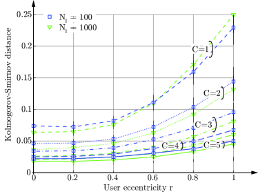
(a) $N_{c}=10$, $\lambda=0.1/{\rm Unit\ Area}$

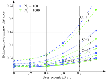
(b) $N_{c}=20$, $\lambda=0.1/{\rm Unit\ Area}$

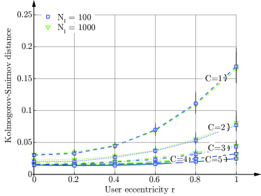
(c) $N_{c}=20$, $\lambda=0.05/{\rm Unit\ Area}$

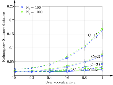
(d) $N_{c}=40$, $\lambda=0.05/{\rm Unit\ Area}$

Figure 4: Kolmogorov-Smirnov distance over user eccentricity $r$. Plot markers $\{\bigtriangledown,\Box\}$ refer to various scenario sizes $N_{\rm I}=\{100,1\,000\}$ expected interferers, respectively. Different line styles denote circular models with $C=\{1,2,3,4,5\}$. Figure labels refer to the corresponding number of nodes per circle, $N_{c}$, and the density $\lambda$ of the original interferer deployment. Black bars depict $95\%$ confidence intervals.

For each scenario snapshot, ten circular models with $C=\{1,2,3,4,5\}$ and two distinct values of $N_{c}$ are set up according to section IV-A. In the case of $\lambda=0.1/{\rm Unit\ Area}$, $N_{c}=\{10,20\}$ and, for $\lambda=0.05/{\rm Unit\ Area}$, $N_{c}=\{20,40\}$, respectively. Then, the aggregate interference distributions are determined. The distributions for the original interferer deployment are only obtained via simulations (by averaging over $1\,000$ spatial realizations and $10\,000$ fading realizations), since the vast amount of nodes hampers the application of Theorem III.1 due to complexity issues. On the other hand, the circular models comprise at most $44$ active nodes and therefore enable to utilize the theorem. This number is obtained for $C=5$ and $N_{c}=40$, and stems from the fact that in a homogeneous BS deployment, the dominant interferers are also the closest ones. Therefore, the presented scheme only maps a single BS on each circle $c<C$, i.e., except for $c=C$ there is only one active node per circle.

fig. 4 depicts Kolmogorov-Smirnov distances over the user eccentricity $r$. The first important observation is that the accuracy considerably improves with an increasing number of circles $C$. This mainly results from accurately capturing the first few dominant BSs that have the largest impact on the aggregate interference distribution, as later shown in section V. A second remarkable observation is that doubling the amount of nodes per circle from $N_{c}=10$ to $N_{c}=20$ for $\lambda=0.1/{\rm Unit\ Area}$ (conf. 4a and 4b), and from $N_{c}=20$ to $N_{c}=40$ for $\lambda=0.05/{\rm Unit\ Area}$ (conf. 4c and 4d) does not achieve smaller Kolmogorov-Smirnov distances, respectively. This result indicates that it is rather the number of circles $C$ than the number of nodes per circle $N_{c}$ that impacts the accuracy. As shown in the examples, good operating points are $N_{c}=\lfloor 1/\lambda\rfloor$ and $C={\rm arg\,min}_{c}|\ell(d_{c})/\ell(d_{1})-2\,\lambda|$, where $d_{c}$ denotes the average distance of the $c$-th dominant interferer to the origin [37]. Lastly, it should be noted that the circular model allows to represent $1\,000$ and more interferers by some $10$ nodes with Kolmogorov-Smirnov distances at the cell-edge not exceeding $0.05$.

IV-C Performance Evaluation of Heterogeneous Base Station Deployments

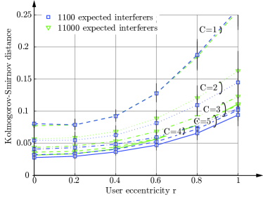
(a) $N_{c}=10$

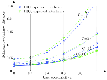
(b) $N_{c}=20$

Figure 5: Kolmogorov-Smirnov distance over user eccentricity $r$ for heterogeneous PPP scenarios with $\lambda=0.1/{\rm UnitArea}$ ($P_{T1}=1$) and $\lambda_{2}=1/{\rm Unit\ Area}$ ($P_{T2}=0.01$). Plot markers $\{\bigtriangledown,\Box\}$ refer to various scenario sizes with $\{1\,100,11\,000\}$ expected interferers, respectively. Different line styles denote circular models with $C=\{1,2,3,4,5\}$. Figure labels refer to the corresponding number of nodes per circle $N_{c}$. Black bars depict $95\%$ confidence intervals.

In this section, a second independent PPP of intensity $\lambda_{2}=1/{\rm Unit\ Area}$ is added on top of the PPP scenarios with $\lambda=0.1$ in section IV-B. The corresponding nodes transmit with normalized power $P_{T2}=0.01$, thus representing a dense overlay of low power BSs. For simplicity, they are distributed within annuli of inner radius $R_{\rm in}$ and outer radii $R_{\rm out}$ as specified above. Then, the total number of expected interferers calculates as $\{1\,100,11\,000\}$, respectively. For each snapshot, algorithm 1 is applied with $C=\{1,2,3,4,5\}$ and $N_{c}=\{10,20\}$. The performance evaluation is carried out along the lines of section IV-B and the parameters are summarized in table II.

fig. 5 depicts the results in terms of Kolmogorov Smirnov distances. It is observed that employing the same parameters $C$ and $N_{c}$ as for the homogeneous scenarios only slightly decreases the performance (conf. 4a and 4b), although mapping $11$ times as many interferers. Hence, applying the recommendations in section IV-B with respect to the PPP that models the BSs with the highest power, yields a good initial operating point.

IV-D Power Profiles of PPP Snapshots

As indicated in fig. 3, power profiles of homogeneous PPP scenarios are characterized by one or a few large amplitudes. To quantify this claim, fig. 6 shows the empirical distributions of the power-profile peak-to-average ratios as obtained from the PPPs in section IV-B with $\lambda=0.1/{\rm Unit\ Area}$. The corresponding circular models encompass a single circle (i.e., $C=1$) with $N_{1}=20$ mapping points. It is observed that the peak-to-average ratios range from $3$ to $19$ with the medians being located around $9.5$. The presence of dominant interferers results in a large asymmetry of the interference impact. However, in modeling approaches that are based on stochastic geometry, the differences between scenarios at both ends of the scale are concealed by spatial averaging. What is more, such approaches commonly require user-centric isotropy of the setup in order to obtain exact solutions (e.g., circularly symmetric exclusion regions [31]). Hence, the differences between interference characteristics in the center of the cell and at cell-edge are generally not accessible. The next section applies the circular model to generate a generic, circularly symmetric scenario and, by employing Theorem III.1, analyzes the impact of user eccentricity.

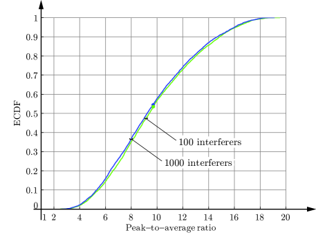
Figure 6: Peak-to-average ratio of power profiles of PPP scenarios with intensity $\lambda=0.1/{\rm Unit\ Area}$ and $N_{\rm I}=\{100,1000\}$ expected interferers. The corresponding circular models are obtained by algorithm 1 with $C=1$ and $N_{1}=20$. Bold dots denote the mean ratios.

V Interference and Rate at Eccentric User Locations

This section investigates user-centric BS collaboration schemes in scenarios with asymmetric interferer impact. The asymmetry can either arise from non-uniform power profiles or user locations outside the center of an otherwise isotropic scenario. The particular emphasis of this section is on the latter, since it is found less frequently in literature. In order to generate a generic, circularly symmetric scenario, the introduced circular model is applied, which enables to employ Theorem III.1 for the analysis of the interference statistics.

V-A Generic Circularly Symmetric Scenario

The network is composed of a central BS and two circles of interferers with $R_{1}=2$ and $R_{2}=4$, as depicted in fig. 7. Each circle employs $10$ interferers, a uniform power profile, i.e., $p_{c}[n]=1/10$, and unit total transmit power, i.e., $P_{c}=1$. The interferer locations are assumed to be rotated by $\phi_{1}=-\pi/10$ and $\phi_{2}=0$, respectively. BS $\mathcal{T}_{0,0}$ is located at the origin and $P_{0}=0.1$. The normalized system parameters are employed to emulate a unit central cell size and to facilitate reproducibility.

The parameters of the circular model are summarized in table III and the modeling of the signal propagation is referred from table II, respectively. The first goal is to identify the nodes, which dominate the interference statistics at eccentric user locations. Then, these insights are applied for user-centric BS coordination and -cooperation.

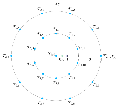
Figure 7: Circular model with two two circles of radius $R_{1}=2$ and $R_{2}=4$, respectively. Each circle employs $10$ transmitters. The transmitter positions are rotated by $\phi_{1}=-\pi/10$ and $\phi_{2}=0$. Users at $r=0.5$ and $r=1$ are denoted as bold dots and refer to middle of cell and cell-edge, respectively.

V-B Components of Asymmetric Interference

TABLE III: Parameters of circular model for numerical evaluation.

Circle	Values
1	$R_{1}=2$	$N_{1}=10$	$P_{1}=1$	$\phi_{1}=-\frac{\pi}{10}$	$p_{1}[n]=\frac{1}{10}$	$n\in\{1,\ldots,10\}$
2	$R_{2}=4$	$N_{2}=10$	$P_{2}=1$	$\phi_{2}=0$	$p_{2}[n]=\frac{1}{10}$	$n\in\{1,\ldots,10\}$

In the first step, only the inner circle of interferers is assumed to be present, i.e., the set $\mathcal{I}$ comprises the $10$ nodes $\mathcal{T}_{1,n},\,n=1,\ldots,10$, of circle $1$. The target is to determine the impact of the closest nodes on the aggregate interference statistics. For this purpose, two representative user locations at $r=R_{1}/4$ and $r=R_{1}/2$ are investigated, referring to middle of cell and cell-edge, respectively.

The PDF of the aggregate interference is obtained by Theorem III.1. Its evaluation is simplified by the scenario’s symmetry about the $x$-axis: (i) equal node-to-user distances from upper- and lower semicircle, i.e., $d_{1,n}=d_{1,10-n+1}$, (ii) uniform power profile $p_{1}(n)=1/10$, and (iii) equal scale parameters $\theta_{1,n}=1$. Thus, $\theta^{\prime}_{1,n}(r)=\theta^{\prime}_{1,10-n+1}(r)$, with $\theta^{\prime}_{1n}(r)=P_{1}/10\,\ell(d_{1,n}(r))$. The vectors $\boldsymbol{\theta}_{\mathcal{I}}(r)$ and $\mathbf{k}_{\mathcal{I}}$ are of length $L^{\mathcal{I}}=5$, with $\left[\boldsymbol{\theta}_{\mathcal{I}}(r)\right]_{l}=\theta^{\prime}_{1,l}(r)$ and $\left[\mathbf{k}_{\mathcal{I}}\right]_{l}=4$, respectively. Hence, the distribution of aggregate interference at distance $r$ from the center formulates as

$$f_{I}(x;r)=\sum_{l=1}^{5}\frac{\Lambda_{l}}{\theta^{\prime}_{1,l}(r)^{4}}h_{3,l}(0)e^{-x/\theta^{\prime}_{1,l}(r)},$$ (15)

where

$$\Lambda_{l} =-\frac{1}{6}\prod_{i=1,i\neq l}^{5}\left(1-\frac{\theta_{i}}{\theta_{l}}\right)^{-4},\qquad l=1,\ldots,5,$$ (16)

$$h_{3,l} =\left(h_{1,l}(0)\right)^{3}+3h_{1,l}(0)h_{1,l}^{(1)}(0)+h_{1,l}^{(2)}(0),$$ (17)

with

$$h_{1,l}(0) =-y+4\sum_{i=1,i\neq l}^{5}\left(\frac{1}{\theta_{i}}-\frac{1}{\theta_{l}}\right)^{-1},$$ (18)

$$h_{1,l}^{(1)}(0) =4\sum_{i=1,i\neq l}^{5}\left(\frac{1}{\theta_{i}}-\frac{1}{\theta_{l}}\right)^{-2},$$ (19)

$$h_{1,l}^{(2)}(0) =8\sum_{i=1,i\neq l}^{5}\left(\frac{1}{\theta_{i}}-\frac{1}{\theta_{l}}\right)^{-3}.$$ (20)

fig. 8 shows $f_{I}(x;r)$ for $r=0.5$ (narrow solid curve) and $r=1$ (wide solid curve), referring to middle of cell and cell-edge, respectively. The dots denote results as obtained with the approach in [10], which requires numerical evaluation of a line-integral and confirms the accuracy of the proposed finite-sum representation.

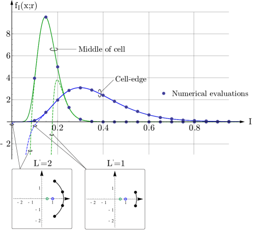
Figure 8: Distribution of aggregate interference at user distances $r=0.5$ and $r=1$, respectively. Dots refer to results as obtained with the approach in [10]. Dashed curves show contribution from dominant interferers.

In eq. 15, each sum term refers to a pair of transmitters $\{\mathcal{T}_{1,l},\,\mathcal{T}_{1,10-l+1}\}$. The contribution of each pair to the final PDF is rendered visible by truncating the sum in eq. 15 at $L^{\prime}$ with $L^{\prime}\in\{1,\ldots,5\}$, i.e., only the first $L^{\prime}$ sum terms are taken into account. Dashed curves in fig. 8 depict results for $L^{\prime}=1$ and $L^{\prime}=2$.

It is observed that (i) in the middle of the cell, body and tail of the PDF are mainly shaped by the four closest interferers while (ii) at cell-edge the distribution is largely dominated by the two closest interferers, and (iii) interference at $r=1$ yields a larger variance than at $r=0.5$ due to higher diversity of the transmitter-to-user distances. The results verify link-level simulations in [40]. They emphasize the strong impact of interference asymmetry due to an eccentric user location, which is commonly overlooked in stochastic geometry analysis. The next section exploits the above findings for BS coordination and -cooperation and investigates the resulting SIR- and rate statistics.

V-C Transmitter Collaboration Schemes

This subsection studies SIR- and rate statistics in the full two-circle scenario, as shown in fig. 7. Motivated by the observations in section V-B, three schemes of BS collaboration are discussed:

1. No collaboration among nodes: This scenario represents the baseline, where $\mathcal{S}=\{\mathcal{T}_{0,0}\}$ and $\mathcal{I}$ comprises all nodes on the circle, i.e., $\mathcal{I}=\{\mathcal{T}_{c,n}\}$ with $c=1,2$ and $n\in\{1,\ldots,10\}$.

2. Interference coordination: The nodes coordinate such that co-channel interference from the two strongest interferers of the inner circle, $\mathcal{T}_{1,1}$ and $\mathcal{T}_{1,10}$, is eliminated. This could be achieved, e.g., by joint scheduling. Then, $\mathcal{S}=\{\mathcal{T}_{0,0}\}$ and $\mathcal{I}$ is composed of $\{\mathcal{T}_{1,n}\}$ with $n\in\{2,\ldots,9\}$ and $\{\mathcal{T}_{2,n}\}$ with $n\in\{1,\ldots,10\}$.

3. Transmitter cooperation: The signals from the two closest nodes of the inner circle, $\mathcal{T}_{1,1}$ and $\mathcal{T}_{1,10}$, can be exploited as useful signals and are incoherently combined with the signal from $\mathcal{T}_{0,0}$. Then, $\mathcal{S}=\{\mathcal{T}_{0,0},\mathcal{T}_{1,1},\mathcal{T}_{1,10}\}$ and, as above, $\mathcal{I}$ comprises $\{\mathcal{T}_{1,n}\}$ with $n\in\{2,\ldots,9\}$ and $\{\mathcal{T}_{2,n}\}$ with $n\in\{1,\ldots,10\}$.

For each collaboration scheme, the PDFs of aggregate signal and -interference, $f_{S}(x;r)$ and $f_{I}(x;r)$, are calculated using Theorem III.1. The SIR at user location $(r,0)$ is defined as $\gamma(r)={S(r)}/{I(r)}$. According to [20], the PDF of $\gamma(r)$ is calculated as

$$f_{\gamma}(\gamma;r)=\int_{0}^{\infty}zf_{S}(z\,\gamma;r)f_{I}(z;r)dz,$$ (21)

where $z$ is an auxiliary variable, $f_{S}(\cdot;r)$ and $f_{I}(\cdot;r)$ refer to eqs. 10 and 11, and the integration bounds are obtained by exploiting the fact that $f_{S}(\gamma;r)=0$ and $f_{I}(\gamma;r)=0$ for $x<0$.

Evaluating eqs. 10 and 11 yields sums of elementary functions of the form $a\gamma^{b}e^{-c\gamma}$, with the generic parameters $a\in\mathbb{R}$, $b\in\mathbb{N}^{+}$ and $c>0$. Therefore, $f_{S}(\gamma;r)$ and $f_{I}(\gamma;r)$ can generically be written as

$$f_{S}(\gamma;r) =\sum_{s}a_{s}\gamma^{b_{s}}e^{-c_{s}\gamma},$$ (22)

$$f_{I}(\gamma;r) =\sum_{i}a_{i}\gamma^{b_{i}}e^{-c_{i}\gamma},$$ (23)

and allow to straightforwardly evaluate eq. 21 as

$$f_{\gamma}(\gamma;r) =\sum_{s}\sum_{i}\int_{0}^{\infty}z\,a_{s}(z\gamma)^{b_{s}}e^{-c_{s}(\gamma z)}\,a_{i}z^{b_{i}}e^{-c_{i}z}dz$$

$$=\sum_{s}\sum_{i}a_{s}a_{i}\gamma^{b_{s}}(c_{i}+c_{s}\gamma)^{-i-b_{s}-b_{i}}\Gamma(i+b_{s}+b_{i}).$$ (24)

The normalized rate $\tau$ as a function of the SIR $\gamma(r)$ is calculated by the well known Shannon formula $\tau(\gamma(r))=\log_{2}\left(1+\gamma(r)\right)$. Note that $\tau(\cdot)$ is a function of the RV $\gamma(r)$. Hence, its distribution is calculated by the transformation

$$f_{\tau}(\tau;r)=\log_{e}(2)2^{\tau}f_{\gamma}(2^{\tau}-1;r),$$ (25)

with $f_{\gamma}(\cdot;\cdot)$ from eq. 24.

The distributions $f_{\gamma}(\gamma;r)$ and $f_{\tau}(\tau;r)$ are analyzed at $r=0.5$ and $r=1$ referring to middle of the cell, and cell-edge, respectively. For reasons of clarity, CDF curves are presented. In order to verify the analysis, Monte Carlo simulations are carried out, employing the system model from section V-A and the signal propagation model from table II. The results are computed by averaging over $10^{7}$ channel realizations for each BS collaboration scheme and each user location, and are denoted as bold dots in figs. 9 and 10, respectively.

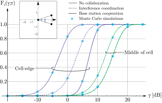
Figure 9: SIR CDF curves for user locations in the middle of the cell ($r=0.5$) and at cell-edge ($r=1$), respectively. Three cases are depicted: (i) No collaboration among BSs (solid), (ii) interference coordination (dashed), (iii) cooperation among BSs (dotted).

fig. 9 shows the obtained SIR distributions. It is observed that

• In the case of no collaboration (solid lines in fig. 9), the curves have almost equal shape in the middle of the cell and at cell-edge. The distribution in the middle of the cell is slightly steeper due to the lower variance of the interferer impact. Their medians, hereafter used to represent the distributions’ position, differ by 15.5 dB.

• When the central node $\mathcal{T}_{0,0}$ coordinates its channel access with the user’s two dominant interferers, $\mathcal{T}_{1,1}$ and $\mathcal{T}_{1,10}$, the SIR improves by 2.4 dB in the middle of the cell and 5.9 dB at cell-edge (dashed curves in fig. 9), compared to no collaboration.

• BS cooperation enhances the SIR by 10.2 dB at cell-edge in comparison to no collaboration (left dotted curve in fig. 9). Note that the CDF curve also has a steeper slope than without coordination, indicating lower variance of the SIR.

• In the middle of the cell, cooperation achieves hardly any additional improvement, as recognized from the overlapping rightmost curves in fig. 9. This remarkable result states that interference coordination already performs close to optimal at this user location. Note that in realistic networks coordination is typically far less complex than cooperation.

The curves reflect findings from [36], stating that even in the best case, gains of transmitter cooperation are much smaller than largely envisioned. fig. 10 depicts the corresponding rate distributions. The results show that

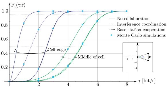
Figure 10: Normalized-rate CDF curves for user locations in the middle of the cell ($r=0.5$) and at cell-edge ($r=1$), respectively. Three cases are depicted: (i) No collaboration among BSs (solid), (ii) interference coordination (dashed), (iii) cooperation among BSs (dotted).

• Notably, the rate statistics of all three collaboration schemes indicate lower variance at cell-edge than in the middle of the cell.

• In terms of median value, BS coordination shows rate improvements by $18.7\,\%$ in the middle of the cell and by $167\,\%$ at cell-edge.

• Cooperation between the central node $\mathcal{T}_{0,0}$ and the user’s two closest interferers, $\mathcal{T}_{1,1}$ and $\mathcal{T}_{1,10}$, achieves a rate enhancement of 19.8 % in the middle of the cell and 355.7 % at cell-edge. Similar to the SIR, it is observed that in the middle of the cell, interference coordination already performs close to optimal.

In summary, collaboration among the BSs that were identified as main contributors to the shape of the interference distribution by Theorem III.1, achieved large performance enhancements in terms of SIR and rate. It was further shown that the efficiency of such schemes considerably depends on the user eccentricity, or equivalently, the asymmetry of the interference impact.

VI Summary and Conclusions

This paper introduced a new interference model that enables to represent substantially large interferer deployments by a well-defined circular structure in terms of interference statistics. The model applies angle-dependent power profiles, which require the specification of a mapping procedure. The presented scheme, despite not claimed to be optimal, achieved to accurately capture heterogeneous interferer deployments with hundreds or even thousands of base stations by a circular model with only several tens of nodes, reducing complexity substantially. Motivated by the desire to decompose the aggregate interference distribution into the contributions from the individual sources, a new representation for the sum of Gamma random variables with integer shape parameter was proposed. The approach enabled to identify candidate base stations for user-centric base station collaboration schemes and to predict the corresponding SIR- and rate statistics at eccentric user locations. It was shown that the performance largely depends on the asymmetry of the interference impact. At the same time, power profiles of PPP scenarios indicated the frequent presence of one or a few dominant interferers. Interference modeling based on stochastic geometry tends to conceal this diversity by spatial averaging and isotropic conditions. The authors are therefore confident that the introduced framework offers a convenient tool for investigating fifth generation mobile cellular networks, where the number of interferers and the diversity of scenarios is expected to grow substantially. Further work is mainly directed towards enhanced mapping schemes.

-A Proof of Theorem III.1

Let $G_{l}\sim\Gamma[k_{l},\theta_{l}]$ be $L$ independent random variables with $k_{l}$ being positive integers and all $\theta_{l}$ different. Then, the PDF of $Y=\sum_{l=1}^{L}G_{l}$ can be expressed as [10]

$$f_{Y}(y) =\left(\prod_{i=1}^{L}\frac{1}{\theta_{i}^{k_{i}}}\right)\frac{1}{2\pi\imath}\oint_{C}\frac{\prod_{i=1}^{L}\left\{\Gamma\left(\frac{1}{\theta_{i}}+s\right)\right\}^{k_{i}}}{\prod_{i=1}^{L}\left\{\Gamma\left(1+\frac{1}{\theta_{i}}+s\right)\right\}^{k_{i}}}e^{sy}ds$$ (26)

$$=\left(\prod_{i=1}^{L}\frac{1}{\theta_{i}^{k_{i}}}\right)\mathcal{G}_{\mathcal{K},\mathcal{K}}^{\mathcal{K},0}\left[e^{-y}\left|\begin{array}[]{l}\boldsymbol{\Theta}_{a}\\ \boldsymbol{\Theta}_{b}\end{array}\right.\right],$$ (29)

where $\mathcal{G}_{p,q}^{m,n}[\cdot]$ denotes Meijer’s G function, $\mathcal{K}=\sum_{i=1}^{L}k_{i}$, and

$$\boldsymbol{\Theta}_{a} =\left\{\overbrace{\left(1+\frac{1}{\theta_{1}}\right),\ldots,\left(1+\frac{1}{\theta_{1}}\right)}^{k_{1}\ {\rm times}},\ldots,\overbrace{\left(1+\frac{1}{\theta_{L}}\right),\ldots,\left(1+\frac{1}{\theta_{L}}\right)}^{k_{L}\ {\rm times}}\right\},$$ (30)

$$\boldsymbol{\Theta}_{b} =\left\{\overbrace{\left(\frac{1}{\theta_{1}}\right),\ldots,\left(\frac{1}{\theta_{1}}\right)}^{k_{1}\ {\rm times}},\ldots,\overbrace{\left(\frac{1}{\theta_{L}}\right),\ldots,\left(\frac{1}{\theta_{L}}\right)}^{k_{L}\ {\rm times}}\right\}.$$ (31)

The unique values of $\boldsymbol{\Theta}_{a}$ and $\boldsymbol{\Theta}_{b}$ and their multiplicities $k_{i}$ are gathered by the vectors $\mathbf{a}$, $\mathbf{b}$ and $\mathbf{k}$, respectively. Then, $|\mathbf{a}|=|\mathbf{b}|=L$, $a_{i}=\left(1+1/\theta_{i}\right)$ and $b_{i}=\left(1/\theta_{i}\right)$ for $i=1,\ldots,L$.

By virtue of the calculus of residues, eq. 26 can be evaluated by a summation over the negative residues of the integrand

$$I(s)=\frac{\prod_{i=1}^{L}\left\{\Gamma\left(\frac{1}{\theta_{i}}+s\right)\right\}^{k_{i}}}{\prod_{i=1}^{L}\left\{\Gamma\left(1+\frac{1}{\theta_{i}}+s\right)\right\}^{k_{i}}}z^{s}$$ (32)

as

$$\mathcal{G}_{\mathcal{K},\mathcal{K}}^{\mathcal{K},0}\left[z\left|\begin{array}[]{l}\boldsymbol{\Theta}_{a}\\ \boldsymbol{\Theta}_{b}\end{array}\right.\right]=-\sum_{l=1}^{L}\sum_{j=0}^{\infty}R_{l}(j).$$ (33)

With

$$R_{l}(j)=\frac{1}{(k_{l}-1)!}\frac{d^{k_{l}-1}}{ds^{k_{l}-1}}\left.\left\{\left(s-\left(\frac{1}{\theta_{l}}+j\right)^{k_{l}}\right)I(s)\right\}\right|_{s=\frac{1}{\theta_{l}}+j}$$ (34)

and the substitution $s=\frac{1}{\theta_{l}}+k+\zeta$, it is obtained

$$R_{l}(j) =\frac{1}{(k_{l}-1)!}\frac{d^{k_{l}-1}}{d\zeta^{k_{l}-1}}g(\zeta;j)=g_{l}(0;j)\frac{h_{k_{l}-1}(0;j)}{(k_{l}-1)!}.$$ (35)

Auxiliary function $g_{l}(0;j)$ is calculated as

$$g_{l}(0;j)= (-1)^{k_{l}}z^{1/\theta_{l}}\frac{\prod_{i=1,i\neq l}^{L}\Gamma(\beta_{i})^{k_{i}}}{\prod_{i=1}^{L}\Gamma(\alpha_{i})^{k_{i}}}\frac{z^{j}}{j!}\frac{\prod_{i=1}^{L}\left((1-\alpha_{i})_{j}\right)^{k_{i}}}{\prod_{i=1,i\neq l}^{L}\left((1-\beta_{i})_{j}\right)^{k_{i}}},$$ (36)

where $(\cdot)_{c}$ refers to the Pochhammer symbol, which is specified as $(x)_{j}=x(x+1)\ldots(x+j-1)$. The therms $\alpha_{i}$ and $\beta_{i}$ are defined as $\alpha_{i}=a_{i}-b_{l}$ and $\beta_{i}=b_{i}-b_{l}$, respectively.

Auxiliary function $h_{\delta,l}(0;j)$ is recursively determined as

$$h_{\delta+1,l}(\zeta;j)=h_{1,l}(\zeta;j)h_{\delta,l}(\zeta;j)+\frac{d}{d\zeta}h_{\delta,l}(\zeta;j).$$ (37)

It is left to provide the expressions for $h_{1,l}(\zeta;j)$ and $h_{1,l}^{(m)}(\zeta;j)$ at $\zeta=0$:

$$h_{1,l}(0;j)= \log(z)-k_{l}\,\psi(1+j)-\sum_{i=k_{l}+1}^{\mathcal{K}}\psi(\beta_{i}-j)+\sum_{i=1}^{\mathcal{K}}\psi(\alpha_{i}-j),$$ (38)

$$h_{1,l}^{(m)}(0;j)= \left.\frac{d^{m}}{d\zeta^{m}}h_{1,l}(\zeta;j)\right|_{\zeta=0}$$

$$= k_{l}\psi^{(m)}(1)-k_{l}\psi^{(m)}(1+j)+(-1)^{m}\left(-k_{l}\psi^{(m)}(1)-\sum_{i=1,i\neq l}^{L}\psi^{(m)}(\beta_{i}-j)+\sum_{i=1}^{L}\psi^{(m)}(\alpha_{i}-j)\right),$$ (39)

where $\psi^{(m)}(z)=\frac{d^{m}}{dz^{m}}\log\left(\Gamma(z)\right)$ refers to the polygamma function of order $m$.

Since $\alpha_{i}=1$ for $i=l$, the argument $(\alpha_{i}-j)$ in eqs. 38 and -A can take on non-positive integer values for $j>1$, where the polygamma function has poles of order $m+1$. These poles are however compensated by the zeros $(1-\alpha_{i})$ in eq. 36 due to the following facts: (i) By definition, $(0)_{c}=0$ for $j\geq 1$, (ii) the zeros are of order $k_{l}$ and (iii) for any non-positive integer $q$

$$\lim\limits_{x\rightarrow q}\,(x-q)^{k_{l}}\psi^{(k_{l}-2)}(x-q)=0,$$ (40)

$$\lim\limits_{x\rightarrow q}\,(x-q)^{k_{l}}\left(\psi^{(0)}(x-q)\right)^{k_{l}-1}=0.$$ (41)

The derivation order $(k_{l}-2)$ and the exponent $k_{l}-1$ in eqs. 40 and 41 correspond to the respective maximum values in $h_{k_{l}-1,l}(0;j)$. Consequently, $R_{l}(j)=0$ for $j>0$ and, therefore, eq. 33 is simplified as

$$\mathcal{G}_{\mathcal{K},\mathcal{K}}^{\mathcal{K},0}\left[z\left|\begin{array}[]{l}\boldsymbol{\Theta}_{a}\\ \boldsymbol{\Theta}_{b}\end{array}\right.\right]=-\sum_{l=1}^{L}R_{l}(0).$$ (42)

$R_{l}(0)$ is composed of $h_{\delta,l}(0;0)$ and $g_{l}(0;0)$.

From eqs. 38 and -A it holds that

$$h_{1,l}(0;0) =\log(z)+\sum_{i=1,i\neq l}^{L}\frac{1}{\beta_{i}},$$ (43)

$$h_{1,l}^{(m)}(0;0) =m!\sum_{i=1,i\neq l}^{L}\left(\frac{1}{\beta_{i}}\right)^{m+1},$$ (44)

where the recurrence relation of the Polygamma function is applied. Simple manipulations yield eqs. 8 and 9. With eq. 7, $h_{\delta,l}(0;0)$ can be derived. Note that in eqs. 8, 9 and 7 the second ”$0$” in the argument, which stems from $j=0$, is omitted for readability.

Considering that $\alpha_{i}=1+\beta_{i}$ and using the recurrence relation $\Gamma(z+1)=z\Gamma(z)$ of the Gamma function, eq. 36 can be simplified as

$$g(0;0)=(-1)^{k_{l}}z^{1/\theta_{l}}\prod_{i=1,i\neq l}^{L}\left(\frac{1}{\beta_{i}}\right)^{k_{i}}.$$ (45)

Finally, eqs. 6 and 5 are obtained from eqs. 43, 44 and 45.

References

- [1] 3GPP. Coordinated multi-point operation for LTE physical layer aspects. TR 36.819, 3rd Generation Partnership Project (3GPP), Sept. 2013.
- [2] 3GPP. Evolved Universal Terrestrial Radio Access (E-UTRA); mobility enhancements in heterogeneous networks. TR 36.839, 3rd Generation Partnership Project (3GPP), Jan. 2013.
- AAK [01] M.-S. Alouini, A. Abdi, and Mostafa Kaveh. Sum of Gamma variates and performance of wireless communication systems over Nakagami-fading channels. IEEE Transactions on Vehicular Technology, 50(6):1471–1480, Nov. 2001.
- ACD+ [12] J.G. Andrews, H. Claussen, M. Dohler, S. Rangan, and M.C. Reed. Femtocells: Past, present, and future. IEEE Journal on Selected Areas in Communications, 30(3):497–508, April 2012.
- ADB [94] Adnan A Abu-Dayya and Norman C Beaulieu. Outage probabilities in the presence of correlated lognormal interferers. IEEE Transactions on Vehicular Technology, 43(1):164–173, Feb. 1994.
- AGH+ [10] J.G. Andrews, R.K. Ganti, M. Haenggi, N. Jindal, and S. Weber. A primer on spatial modeling and analysis in wireless networks. IEEE Communications Magazine, 48(11):156–163, Nov. 2010.
- AHAB [85] Emad K. Al-Hussaini and A. Al-Bassiouni. Performance of MRC diversity systems for the detection of signals with Nakagami fading. IEEE Transactions on Communications, 33(12):1315–1319, Dec. 1985.
- AM [97] S.V. Amari and R.B. Misra. Closed-form expressions for distribution of sum of exponential random variables. IEEE Transactions on Reliability, 46(4):519–522, Dec. 1997.
- APE [05] V.A. Aalo, T. Piboongungon, and G.P. Efthymoglou. Another look at the performance of MRC schemes in Nakagami-m fading channels with arbitrary parameters. IEEE Transactions on Communications, 53(12):2002–2005, Dec. 2005.
- AYAK [12] I.S. Ansari, F. Yilmaz, M.-S. Alouini, and O. Kucur. On the sum of Gamma random variates with application to the performance of Maximal Ratio Combining over Nakagami-m fading channels. In IEEE International Workshop on Signal Processing Advances in Wireless Communications (SPAWC), pages 394–398, June 2012.
- BADM [95] Norman C Beaulieu, Adnan A Abu-Dayya, and Peter J McLane. Estimating the distribution of a sum of independent lognormal random variables. IEEE Transactions on Communications, 43(12):2869–2873, Dec. 1995.
- [12] Francois Baccelli and Bartllomiej Blaszczyszyn. Stochastic Geometry and Wireless Networks: Volume I Theory. Foundation and Trends in Networking. Now Publishers, March 2009.
- [13] François Baccelli and Bartlomiej Blaszczyszyn. Stochastic Geometry and Wireless Networks, Volume II - Applications, volume 2 of Foundations and Trends in Networking. NoW Publishers, 2009.
- BKLZ [97] Fran ois Baccelli, Maurice Klein, Marc Lebourges, and Sergei Zuyev. Stochastic geometry and architecture of communication networks. Telecommunication Systems, 7(1-3):209–227, 1997.
- BLM+ [14] N. Bhushan, Junyi Li, D. Malladi, R. Gilmore, D. Brenner, A. Damnjanovic, R. Sukhavasi, C. Patel, and S. Geirhofer. Network densification: the dominant theme for wireless evolution into 5G. IEEE Communications Magazine, 52(2):82–89, Feb. 2014.
- Bro [00] T.X. Brown. Cellular performance bounds via shotgun cellular systems. IEEE Journal on Selected Areas in Communications, 18(11):2443–2455, Nov. 2000.
- BVH [14] T. Bai, R. Vaze, and R. Heath, Jr. Analysis of blockage effects on urban cellular networks. IEEE Transactions on Wireless Communications, 13(9):5070–5083, Sept. 2014.
- BZ [96] Fran ois Baccelli and Serguei Zuyev. Stochastic geometry models of mobile communication networks. In Frontiers in queueing: models and applications in science and engineering, pages 227–243. CRC Press, 1996.
- Coe [98] Carlos A. Coelho. The generalized integer Gamma distribution - a basis for distributions in multivariate statistics. Journal of Multivariate Analysis, 64(1):86 – 102, 1998.
- Cur [41] J. H. Curtiss. On the distribution of the quotient of two chance variables. The Annals of Mathematical Statistics, 12(4):409–421, 1941.
- DRGC [13] M. Di Renzo, A Guidotti, and G.E. Corazza. Average rate of downlink heterogeneous cellular networks over generalized fading channels: A stochastic geometry approach. IEEE Transactions on Communications, 61(7):3050–3071, July 2013.
- EHH [13] Hesham ElSawy, Ekram Hossain, and Martin Haenggi. Stochastic geometry for modeling, analysis, and design of multi-tier and cognitive cellular wireless networks: A survey. IEEE Communications Surveys & Tutorials, 15(3):996–1019, June 2013.
- EPA [06] G.P. Efthymoglou, T. Piboongungon, and V.A. Aalo. Performance of DS-CDMA receivers with MRC in Nakagami-m fading channels with arbitrary fading parameters. IEEE Transactions on Vehicular Technology, 55(1):104–114, Jan. 2006.
- Ger [12] Jon Gertner. The Idea Factory: Bell Labs and the Great Age of American Innovation. Penguin Group, 2012.
- GH [13] Anjin Guo and Martin Haenggi. Spatial stochastic models and metrics for the structure of base stations in cellular networks. IEEE Transactions on Wireless Communications, 12(11):5800–5812, Oct. 2013.
- GMR+ [12] Amitabha Ghosh, Nitin Mangalvedhe, Rapeepat Ratasuk, Bishwarup Mondal, Mark Cudak, Eugene Visotsky, Timothy A Thomas, Jeffrey G Andrews, Ping Xia, Han Shin Jo, et al. Heterogeneous cellular networks: From theory to practice. IEEE Communications Magazine, 50(6):54–64, June 2012.
- HAB+ [09] M. Haenggi, J.G. Andrews, F. Baccelli, O. Dousse, and M. Franceschetti. Stochastic geometry and random graphs for the analysis and design of wireless networks. IEEE Journal on Selected Areas in Communications, 27(7):1029–1046, Sept. 2009.
- Hae [12] M. Haenggi. Stochastic Geometry for Wireless Networks. Stochastic Geometry for Wireless Networks. Cambridge University Press, 2012.
- HB [05] Jeremiah Hu and Norman C Beaulieu. Accurate simple closed-form approximations to Rayleigh sum distributions and densities. IEEE Communications Letters, 9(2):109–111, Feb. 2005.
- HG [09] Martin Haenggi and Radha Krishna Ganti. Interference in Large Wireless Networks, volume 3 of Foundations and Trends in Networking. NoW Publishers, Feb. 2009.
- HKB [13] Robert W. Heath, Jr., Marios Kountouris, and Tianyang Bai. Modeling heterogeneous network interference using poisson point processes. IEEE Transactions on Signal Processing, 61(16):4114–4126, Aug. 2013.
- IM [13] Serge B. Provost Iman Mabrouk. The exact density function of a sum of independent Gamma random variables as an inverse Mellin transform. International Journal of Applied Mathematics and Statistics, 41(11), 2013.
- Kab [62] D. G. Kabe. On the exact distribution of a class of multivariate test criteria. The Annals of Mathematical Statistics, 33(3):1197–1200, 1962.
- KST [06] G.K. Karagiannidis, N.C. Sagias, and T.A. Tsiftsis. Closed-form statistics for the sum of squared Nakagami-m variates and its applications. IEEE Transactions on Communications, 54(8):1353–1359, Aug. 2006.
- LFR [99] P. Lombardo, G. Fedele, and M.M. Rao. MRC performance for binary signals in Nakagami fading with general branch correlation. IEEE Transactions on Communications, 47(1):44–52, Jan. 1999.
- LHA [13] A. Lozano, R.W. Heath, and J.G. Andrews. Fundamental limits of cooperation. IEEE Transactions on Information Theory, 59(9):5213–5226, Sept. 2013.
- Mol [12] Dmitri Moltchanov. Distance distributions in random networks. Ad Hoc Networks, 10(6):1146–1166, March 2012.
- Mos [85] P.G. Moschopoulos. The distribution of the sum of independent Gamma random variables. Annals of the Institute of Statistical Mathematics, 37(1):541–544, 1985.
- MWMZ [07] Neelesh B Mehta, Jingxian Wu, Andreas F Molisch, and Jin Zhang. Approximating a sum of random variables with a lognormal. IEEE Transactions on Wireless Communications, 6(7):2690–2699, July 2007.
- PDL [06] Simon Plass, Xenofon G. Doukopoulos, and Rodolphe Legouable. Investigations on link-level inter-cell interference in OFDMA systems. In Symposium on Communications and Vehicular Technology (SCVT), pages 49–52, Nov. 2006.
- PK [91] R. Prasad and A Kegel. Improved assessment of interference limits in cellular radio performance. IEEE Transactions on Vehicular Technology, 40(2):412–419, May 1991.
- Pro [89] Serge B. Provost. On sums of independent Gamma random variates. Statistics: A Journal of Theoretical and Applied Statistics, 20(4), 1989.
- RZXZ [13] Chengmeng Ren, Jianfeng Zhang, Wei Xie, and Dongmei Zhang. Performance analysis for heterogeneous cellular networks based on Matern-like point process model. In International Conference on Information Science and Technology (ICIST), pages 1507–1511, March 2013.
- Sch [88] E.M. Scheuer. Reliability of an m-out-of-n system when component failure induces higher failure rates in survivors. IEEE Transactions on Reliability, 37(1):73–74, April 1988.
- TDHA [14] H. Tabassum, Z. Dawy, E. Hossain, and M.-S. Alouini. Interference statistics and capacity analysis for uplink transmission in two-tier small cell networks: A geometric probability approach. IEEE Transactions on Wireless Communications, 13(7):3837–3852, July 2014.
- TKKS [06] T. A. Tsiftsis, G. K. Karagiannidis, S. A. Kotsopoulos, and N. C. Sagias. Performance of MRC diversity receivers over correlated Nakagami- fading channels. In International Symposium of Communication Systems, Networks and Digital Signal Processing (CSNDSP), July 2006.
- TV [12] Don J. Torrieri and Matthew C. Valenti. The outage probability of a finite ad hoc network in Nakagami fading. IEEE Transactions on Communications, 60(11):3509–3518, Nov. 2012.
- TYDA [13] H. Tabassum, F. Yilmaz, Z. Dawy, and M.-S. Alouini. A framework for uplink intercell interference modeling with channel-based scheduling. IEEE Transactions on Wireless Communications, 12(1):206–217, Jan. 2013.
- WA [12] Steven Weber and Jeffrey G. Andrews. Transmission capacity of wireless networks. Foundations and Trends in Networking, 5(2-3):109–281, 2012.
- WPS [09] M.Z. Win, P.C. Pinto, and L.A Shepp. A mathematical theory of network interference and its applications. Proceedings of the IEEE, 97(2):205–230, Feb. 2009.
- Wyn [94] AD. Wyner. Shannon-theoretic approach to a Gaussian cellular multiple-access channel. IEEE Transactions on Information Theory, 40(6):1713–1727, Nov. 1994.
- YC [08] Lie-Liang Yang and Hsiao-Hwa Chen. Error probability of digital communications using relay diversity over Nakagami-m fading channels. IEEE Transactions on Wireless Communications, 7(5):1806–1811, May 2008.
- Zha [98] Q.T. Zhang. Exact analysis of postdetection combining for DPSK and NFSK systems over arbitrarily correlated Nakagami channels. IEEE Transactions on Communications, 46(11):1459–1467, Nov. 1998.