Double Barriers and Magnetic Field in Bilayer Graphene

Ilham Redouani^a, Ahmed Jellal^a,b and Hocine Bahlouli^c

^aTheoretical Physics Group, Faculty of Sciences, Chouaïb Doukkali University,

PO Box 20, 24000 El Jadida, Morocco

^bSaudi Center for Theoretical Physics, Dhahran, Saudi Arabia

^cPhysics Department, King Fahd University of Petroleum and Minerals,
Dhahran 31261, Saudi Arabia

We study the transmission probability in an AB-stacked bilayer graphene of Dirac fermions scattered by a double barrier structure in the presence of a magnetic field. We take into account the full four bands of the energy spectrum and use the boundary conditions to determine the transmission probability. Our numerical results show that for energies higher than the interlayer coupling, four ways for transmission probabilities are possible while for energies less than the height of the barrier, Dirac fermions exhibits transmission resonances and only one transmission channel is available. We show that, for AB-stacked bilayer graphene, there is no Klein tunneling at normal incident. We find that the transmission displays sharp peaks inside the transmission gap around the Dirac point within the barrier regions while they are absent around the Dirac point in the well region. The effect of the magnetic field, interlayer electrostatic potential and various barrier geometry parameters on the transmission probabilities are also discussed.

PACS numbers: 73.22.Pr, 72.80.Vp, 73.63.-b

Keywords: Bilayer graphene, double barriers, magnetic field, transmission.

1 Introduction

Graphene [1] is a single layer of carbon atoms packed in a hexagonal Bravais lattice. This special atomic arrangement gives graphene truly unique and remarkable physical properties. Its thermal conductivity is 15 times larger than that of copper and its electron mobility is 20 times larger than that of GaAs. In addition, graphene is a transparent conductor and has peculiar electronic properties, such as an unusual quantum Hall effect [2, 3] and its conductivity can be modified over a wide range of values either by chemical doping or by applying an electric field. In fact it is the very high mobility of graphene [4] which makes the material very interesting for electronic high speed applications [5]. From the theoretical point of view most of these unusual electronic properties have been associated with the fact that current carrier in graphene are described in terms of massless two-dimensional Dirac particles [6].

For practical applications it has been realized that layered graphene system can play an important role. Hence a few-layer graphene system can be constructed by stacking graphene sheets on top of each other to form a layered graphene. Bilayer graphene, which is of interest to us in this work, is a system consisting of two coupled monolayers of carbon atoms, each with a honeycomb crystal structure [7, 8]. Bilayer graphene has many of the properties that are similar to those of monolayer [6, 9]. For monolayer graphene, one can create an energy gap in the spectrum in many different ways, such as by coupling to substrate or doping with impurities [10, 11], while in bilayer graphene by applying an external electric field [12, 13]. In addition, monolayer graphene has a linear electronic spectrum in the vicinity of the Dirac points. However bilayer graphene has four bands where the lowest conduction band and highest valence band have quadratic spectra, each pair is separated by an interlayer coupling energy of order $\gamma_{1}=0.4\ eV$ [14, 15, 16]. It is well-known that, in the case of monolayer graphene, the electrostatic potential barriers are fully transparent for low energy Dirac fermions at normal incidence, which is referred to as Klein tunneling [17] but for bilayer graphene, no Klein tunneling is expected.

Based on previous investigations of Dirac fermions in bilayer graphene and in particular the work [18] in our recent work [19, 20] we developed a theoretical framework to deal with bilayer graphene in the presence of a perpendicular electric and magnetic fields for single barrier. Our theoretical model is based on the well established tight binding Hamiltonian of graphite [21] and adopted the Slonczewski-Weiss-McClure parametrization of the relevant intralayer and interlayer couplings [22] to model the bilayer graphene system. In the present work, we study the transmission probabilities in AB-stacked bilayer graphene by considering Dirac fermions scattered by double barrier structure in the presence of a magnetic field. By requiring the continuity of the wave functions at interfaces, we find the transmission probabilities. Systematic study revealed that interlayer interaction is essential, in particular the direct interlayer coupling parameter $\gamma_{1}$, for the study of transmission properties. For energies higher than the interlayer coupling, $E>\gamma_{1}$, two propagation modes are available for transport, four possible ways for transmission probabilities are available. While, when the energy is less then the height of the barrier, $E<\gamma_{1}$, the Dirac fermions exhibits transmission resonances and only one mode of propagation is available. This work allowed us to compare our numerical results with existing literature on the subject.

The present paper is organized as follows. In section 2, we formulate our model by setting the Hamiltonian system and determining the associated energy eigenvalues in each potential region. Then, we consider the five potential regions one at a time, we obtain the spinor solution corresponding to each region in terms of barrier parameters and applied fields. In section 3, we use the boundary conditions to calculate the transmission probabilities in terms of different physical parameters. In section 4, we present our numerical results for the transmission probabilities for two cases: when the incident electron energy is either smaller or greater than the interlayer coupling parameter. Finally we conclude our work and discuss its potential importance.

2 Energy spectrum

The considered bilayer graphene system in the presence a perpendicular electric and magnetic fields is shown in Figure 1. The Dirac fermions are scattered by a double barrier potential along the x-direction which results in five different regions. Therefore, the charge carriers in bilayer AB-stacked are described, in each region denoted by $j$ ($j=1,2,3,4,5$), by the following four-band Hamiltonian [6, 23] and the associated eigenspinor $\psi(x,y)$

$$H_{j}=\left(\begin{array}[]{cccc}V^{+}_{j}&v_{F}\pi_{j}^{+}&0&0\\ v_{F}\pi_{j}&V^{+}_{j}&\gamma_{1}&0\\ 0&\gamma_{1}&V^{-}_{j}&v_{F}\pi_{j}^{+}\\ 0&0&v_{F}\pi_{j}&V^{-}_{j}\\ \end{array}\right),\qquad\psi(x,y)=\left(\begin{array}[]{cccc}\psi_{A_{1}}(x,y)\\ \psi_{B_{1}}(x,y)\\ \psi_{A_{2}}(x,y)\\ \psi_{B_{2}}(x,y)\\ \end{array}\right)$$ (1)

where $\pi_{j}=p_{x}+ip_{y}$, $p_{x,y}=-i\hbar\nabla+eA_{j}(x,y)$ is the in-plane momentum relative to the Dirac point, $v_{F}=10^{6}m/s$ is the Fermi velocity. $V^{+}_{j}$ and $V^{-}_{j}$ are the potentials on the first and second layer as defined below

$$V^{\tau}_{j}=\left\{\begin{array}[]{ll}{V_{j}+\tau\delta_{j},}&{j=2,3,4}\\ {0,}&{j=1,5}\end{array}\right.$$ (2)

in the $j$-th region as shown in Figure 1, with $\tau=+1$ ($-1$) on the first layer (second layer), $V_{j}$ is the barrier strength and $\delta_{j}$ is the interlayer electrostatic potential difference.

Figure 1: Schematic diagram for the double barrier, on the first and second layer, in the presence of a magnetic field.

The system is considered to be infinite along the y-direction. In region $j=3$, the magnetic field is chosen to be perpendicular to the graphene sheet along the z-direction and defined as

$$B(x,y)=B\Theta\left[(d_{2}-x)(d_{3}-x)\right]$$ (3)

where $B$ is constant and $\Theta$ is the Heaviside step function. In the Landau gauge, the corresponding vector potential $A(x,y)=(0,A_{y}(x))$ takes the form

$$A_{y}(x)=\frac{\hbar}{el_{B}^{2}}\left\{\begin{array}[]{lllll}{d_{2}},&\mbox{if}&{x<d_{2}}\\ {x},&\mbox{if}&{d_{2}<x<d_{3}}\\ {d_{3}},&\mbox{if}&{x>d_{4}}\\ \end{array}\right.$$ (4)

$l_{B}=\sqrt{\hbar/eB}$ is the magnetic length and $e$ the electronic charge.

In order to solve the eigenvalue problem we can separate variables and write the eigenspinors as plane waves in the y-direction. This is due to the fact that $[H,p_{y}]=0$ requires the conservation of momentum along the y-direction, then we can write $\phi(x,y)=e^{ik_{y}y}\psi(x,k_{y})$. Using the eigenvalue equation $H\psi(x,k_{y})=E\psi(x,k_{y})$, we obtain the following second-order differential equation for $\psi_{B_{1}}(x,k_{y})$

$$\left[2\vartheta_{0}^{2}aa^{\dagger}-\left(E-V_{j}+\delta_{j}\right)^{2}\right]\left[2\vartheta_{0}^{2}a^{\dagger}a-\left(E-V_{j}-\delta_{j}\right)^{2}\right]\psi_{B_{1}}=\gamma_{1}^{2}\left[\left(E-V_{j}\right)^{2}-\delta_{j}^{2}\right]\psi_{B_{1}}$$ (5)

where $\vartheta_{0}=\frac{\hbar v_{F}}{l_{B}}$ is the energy scale. We have introduced the annihilation and creation operators

$$a=\frac{l_{B}}{\sqrt{2}}\left(\partial_{x}+k_{y}+\frac{e}{\hbar}A_{y}(x)\right),\qquad a^{\dagger}=\frac{l_{B}}{\sqrt{2}}\left(-\partial_{x}+k_{y}+\frac{e}{\hbar}A_{y}(x)\right)$$ (6)

which fulfill the commutation relation $\left[a,a^{\dagger}\right]=1.$ In the forthcoming analysis, we solve the above equation each region.

In region $3$ ($d_{2}<x<d_{3})$, the vector potential $A_{y}(x)$ is given by $\frac{\hbar}{el_{B}^{2}}x$. Using the envelope function $\psi_{B_{1}}(x,k_{y})\equiv\psi_{B_{1}}(X)$, where $X=\frac{x}{l_{B}}+k_{y}l_{B}$, (5) becomes

$$\left[-\partial_{X}^{2}+X^{2}-1-2\lambda_{+}\right]\left[-\partial_{X}^{2}+X^{2}-1-2\lambda_{-}\right]\psi_{B_{1}}(X)=0$$ (7)

where we have set

$$\lambda_{\tau}=-\frac{1}{2}+\frac{(E-V_{3})^{2}+\delta_{3}^{2}}{2\vartheta_{0}^{2}}+\tau\frac{\sqrt{(\vartheta_{0}^{2}-2(E-V_{3})\delta_{3})^{2}+\gamma_{1}^{2}((E-V_{3})^{2}-\delta_{3}^{2})}}{2\vartheta_{0}^{2}}.$$ (8)

We solve (7) to obtain the energy in this region as

$$E = V_{3}+\frac{1}{\sqrt{6}}\left[\pm\left[\mu^{\frac{1}{3}}+(A^{2}+3C)\mu^{\frac{-1}{3}}+2A\right]^{\frac{1}{2}}\right.$$

$$\left.\pm\left[-6B\sqrt{6}\left(\mu^{\frac{1}{3}}+(A^{2}+3C)\mu^{\frac{-1}{3}}+2A\right)^{\frac{-1}{2}}-\left(\mu^{\frac{1}{3}}+(A^{2}+3C)\mu^{\frac{-1}{3}}-4A\right)\right]^{\frac{1}{2}}\right]$$

where we have defined the following quantities

$${\mu=-A^{3}+27B^{2}+9AC+3\sqrt{3}\left[-\left(A^{2}+3C\right)^{3}+\left(-A^{3}+27B^{2}+9AC\right)^{2}\right]^{\frac{1}{2}}}$$ (10)

$${A=\delta_{3}^{2}+(2n+1)\vartheta_{0}^{2}+\frac{\gamma_{1}^{2}}{2}}$$ (11)

$${B=\vartheta_{0}^{2}\delta_{3}}$$ (12)

$${C=\left((2n+1)\vartheta_{0}^{2}-\delta_{3}^{2}\right)^{2}-\vartheta_{0}^{4}+\gamma_{1}^{2}\delta_{3}^{2}}$$ (13)

$n$ is an integer number, with $n=\lambda_{\tau}$. It is important to note that when $\gamma_{1}\longrightarrow 0$, the energy will be reduced to the case of a monolayer graphene.

In region $j=1,2,4,5$, the associated vector potential $A_{y}(x)$ is constant and equal to $\frac{\hbar}{el_{B}^{2}}d$ with

$$d=\left\{\begin{array}[]{lll}{d_{2}},&\mbox{if}&{x<d_{2}}\\ {d_{3}},&\mbox{if}&{x>d_{3}}.\\ \end{array}\right.$$ (14)

The corresponding energy can be written as

$$E-V_{j}=\pm\sqrt{\left(\hbar v_{F}k_{j}\right)^{2}+\frac{\gamma_{1}^{2}}{2}+\delta_{j}^{2}\pm\sqrt{\left(\hbar v_{F}k_{j}\right)^{2}(\gamma_{1}^{2}+4\delta_{j}^{2})+\frac{\gamma_{1}^{4}}{4}}}$$ (15)

and the wave vector $k_{j}$ is

$$k_{j}=\sqrt{\left(\alpha_{j}^{\pm}\right)^{2}+\left(k_{y}+\frac{d}{{l_{B}}^{2}}\right)^{2}}.$$ (16)

In the incident region $\alpha_{1}^{\pm}$ being the wave vector of the propagating wave, where there are two right-going propagating modes and two left-going propagating modes. For the transmission region, $\alpha_{5}^{\pm}$ is the wave vector of the propagating wave with two right-going propagating modes.

3 Transmission probability

Next we will calculate the transmission probability of electrons across the double potential barrier in our AB-stacked bilayer graphene system. In doing so, we follow two steps where firstly we write our obtained eigenspinors in matrix notation and secondly we impose the continuity of the wave function at each potential interface.

Recall that our eigenspinors can be obtained in similar way as we have done in [20] dealing with the same system but scattered by single barrier potential. To go further, it is convenient to use the matrix formalism such that the wave function in each region, denoted by the integer $j$, can then be writhen as

$$\psi_{j}=G_{j}\cdot M_{j}\cdot A_{j}$$ (17)

where $A_{1}$ and $A_{5}$

$$A_{1}^{\tau}=\left(\begin{array}[]{c}\delta_{\tau,1}\\ r_{+}^{\tau}\\ \delta_{\tau,-1}\\ r_{-}^{\tau}\\ \end{array}\right),\qquad A_{5}^{\tau}=\left(\begin{array}[]{c}t_{+}^{\tau}\\ 0\\ t_{-}^{\tau}\\ 0\\ \end{array}\right)$$ (18)

are given in terms of the transmission $t_{\pm}^{\tau}$ and reflection $r_{\pm}^{\tau}$ amplitudes as well as the Kronecker delta symbol $\delta_{\tau,\pm 1}$. For the remanning regions, we have

$$A_{2,3,4}=\left(\alpha_{2,3,4},\alpha_{2,3,4}^{{}^{\prime}},\beta_{2,3,4},\beta_{2,3,4}^{{}^{\prime}}\right)^{T}$$ (19)

where the appearing coefficients are coming from the decomposition of the eigenspinors in different regions. In regions $j=1,\ 2,\ 4,\ 5$, $G_{j}$ and $M_{j}$ take the forms

$$G_{j}=\left(\begin{array}[]{cccc}f_{j}^{++}&f_{j}^{+-}&f_{j}^{-+}&f_{j}^{--}\\ 1&1&1&1\\ h_{j}^{+}&h_{j}^{+}&h_{j}^{-}&h_{j}^{-}\\ g_{j}^{+-}&g_{j}^{++}&g_{j}^{--}&g_{j}^{-+}\\ \end{array}\right),\qquad M_{j}=\left(\begin{array}[]{cccc}e^{i\alpha_{j}^{+}x}&0&0&0\\ 0&e^{-i\alpha_{j}^{+}x}&0&0\\ 0&0&e^{i\alpha_{j}^{-}x}&0\\ 0&0&0&e^{-i\alpha_{j}^{-}x}\\ \end{array}\right)$$ (20)

with the quantities

$$f_{j}^{\tau\pm}=\hbar v_{F}\left(\pm\alpha_{j}^{\tau}-i\left(k_{y}+\frac{d}{l_{B}^{2}}\right)\right)/\left(E-V_{j}-\delta_{j}\right)$$ (21)

$$h_{j}^{\tau}=\frac{E-V_{j}-\delta_{j}}{\gamma_{1}}\left[1-\frac{\left(\hbar v_{F}\right)^{2}\left[\left(\alpha_{j}^{\tau}\right)^{2}+\left(k_{y}+\frac{d}{l_{B}^{2}}\right)^{2}\right]^{2}}{\left(E-V_{j}-\delta_{j}\right)^{2}}\right]$$ (22)

$$g_{j}^{\tau\pm}=-\frac{E-V_{j}-\delta_{j}}{E-V_{j}+\delta_{j}}h_{j}^{\tau}f_{j}^{\tau\pm}.$$ (23)

In region $j=3$, we have $G_{3}=\mathbb{I}_{4}$ and $M_{3}$ reads as

$$M_{3}=\left(\begin{array}[]{cccc}\eta_{-}\lambda_{+}\chi_{-1}^{++}&\eta_{-}^{*}\lambda_{+}\chi_{-1}^{+-}&\eta_{-}\lambda_{-}\chi_{-1}^{-+}&\eta_{-}^{*}\lambda_{-}\chi_{-1}^{--}\\ \chi_{0}^{++}&\chi_{0}^{+-}&\chi_{0}^{-+}&\chi_{0}^{--}\\ \zeta^{+}\chi_{0}^{++}&\zeta^{+}\chi_{0}^{+-}&\zeta^{-}\chi_{0}^{-+}&\zeta^{-}\chi_{0}^{--}\\ \eta_{+}^{*}\zeta^{+}\chi_{1}^{++}&\eta_{+}\zeta^{+}\chi_{1}^{+-}&\eta_{+}^{*}\zeta^{-}\chi_{1}^{-+}&\eta_{+}\zeta^{-}\chi_{1}^{--}\end{array}\right)$$ (24)

where we have set

$$\eta_{\pm}=\frac{-i\sqrt{2}\vartheta_{0}}{E-V_{3}\pm\delta_{3}}$$ (25)

$$\zeta^{\tau}=\frac{E-V_{3}-\delta_{3}}{\gamma_{1}}-\frac{2\vartheta_{0}^{2}\lambda_{\tau}}{\gamma_{1}\left(E-V_{3}-\delta_{3}\right)}$$ (26)

$$\chi_{l}^{\tau\pm}=D\left[\lambda_{\tau}+l,\pm\sqrt{2}X\right]$$ (27)

$D\left[\lambda_{\tau}+l,\pm\sqrt{2}X\right]$ are the parabolic cylindrical functions with the quantum numbers $\lambda_{\tau}=n$ and $l=0,\pm 1.$

Now let us consider the boundary conditions at $x=d_{j}$ and then from (17) we end up with the set of equations

$${G_{1}\cdot M_{1}[x=d_{1}]\cdot A_{1}^{\tau}=G_{2}\cdot M_{2}[x=d_{1}]\cdot A_{2}}$$ (28)

$${G_{2}\cdot M_{2}[x=d_{2}]\cdot A_{2}=G_{3}\cdot M_{3}[x=d_{2}]\cdot A_{3}}$$ (29)

$${G_{3}\cdot M_{3}[x=d_{3}]\cdot A_{3}=G_{4}\cdot M_{4}[x=d_{3}]\cdot A_{4}}$$ (30)

$${G_{4}\cdot M_{4}[x=d_{4}]\cdot A_{4}=G_{5}\cdot M_{5}[x=d_{4}]\cdot A_{5}^{\tau}}.$$ (31)

Using the transfer matrix method we can connect $A_{1}^{\tau}$ with $A_{5}^{\tau}$ through the matrix $N$

$$N=\prod_{j=1}^{4}M_{j}^{-1}[x=d_{j}]\cdot G_{j}^{-1}\cdot G_{j+1}\cdot M_{j+1}[x=d_{j}]$$ (32)

which can help to explicitly determine $t_{\pm}^{\tau}$ and therefore the corresponding transmission probability, in a compact form, as

$$T_{\pm}^{\tau}=\frac{\alpha_{2}^{\pm}}{\alpha_{1}^{\tau}}\mid t_{\pm}^{\tau}\mid^{2}.$$ (33)

In next section, we will study numerically two interesting cases depending on the value of the incident energies, $E$, as compared with the interlayer coupling parameter $\gamma_{1}$. The two band tunneling leads to one transmission and one reflection channel and takes place at energies less than the interlayer coupling, $E<\gamma_{1}$. On the other hand, for energies higher than the interlayer coupling parameter $\gamma_{1}$, $E>\gamma_{1}$, the four band tunneling takes place giving rise to four transmission and four reflection channels.

4 Numerical results

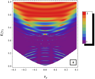
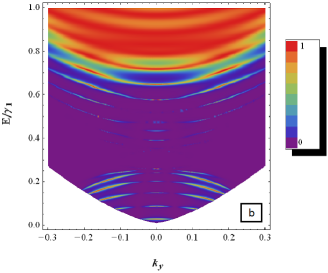
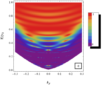
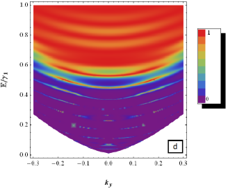
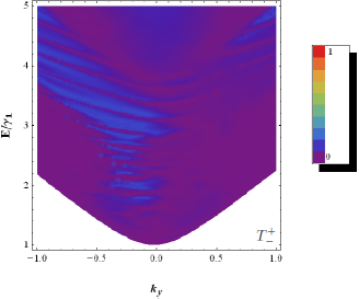
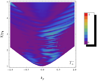
We compute numerically the transmission probability through the double barrier in the presence of a magnetic field in the low energy regime. The two band model only allows for one mode of propagation, leading to one transmission. In this case, Figure 2 shows the density plot of the transmission probability as a function of the transverse wave vector $k_{y}$ and energy $E$. Figures (2a) and (2c) present two different structures of the double barrier. In Figure (2a), we show that the transmission for $V_{2}=V_{4}=0.6\ \gamma_{1}$, $V_{3}=0.3\ \gamma_{1}$ and $\delta_{2}=\delta_{3}=\delta_{4}=0\ \gamma_{1}$. At nearly normal incidence ($k_{y}\approx-\frac{d_{2}}{l_{B}^{2}}$ and $k_{y}\approx-\frac{d_{3}}{l_{B}^{2}}$) the transmission is zero and there are no resonances in the low regime energy $E<V_{3}$. While resonances occur at non-normal incidence, which is equivalent to the case of a single barrier [20]. In the regime of energy $V_{3}<E<V_{2}=V_{4}$, it is clearly seen that the peaks are due to the bound electron states [19]. In addition, when $E>V_{2}=V_{4}$ the Dirac fermions exhibit transmission resonances. While many of these results are similar to those obtained in Figure (2c), with $V_{3}=\delta_{3}=0\ \gamma_{1}$. It is important to see how the interlayer potential difference and the resulting energy gap in the energy spectrum affect the transmission probability. To answer this inquiry we give the results presented in Figures (2b) and (2d). We notice that in Figure (2b), the transmission displays sharp peaks inside the transmission gap around the Dirac point $E=V_{2}=V_{4}$, that are absent around $E=V_{3}$. As observed in Figure (2d) the transmission probability displays sharp peaks around the only Dirac point at $E=V_{2}=V_{4}$. It is clearly seen that the displayed sharp peaks inside the transmission gap for a double barrier structure do not appear in the case for the single barrier [20].

Figure 2: Density plot of transmission probability as a function of the transverse wave vector $k_{y}$ and its energy $E$, for $d_{4}=-d_{1}=30\ nm$, $d_{3}=-d_{2}=20\ nm$ and $l_{B}=18.5\ nm$. (a): $V_{2}=V_{4}=0.6\ \gamma_{1}$, $V_{3}=0.3\ \gamma_{1}$ and $\delta_{2}=\delta_{3}=\delta_{4}=0\ \gamma_{1}$. (b): the same parameters as in (a) with $\delta_{2}=\delta_{4}=0.1\ \gamma_{1}$ and $\delta_{3}=0.05\ \gamma_{1}$. (c): $V_{2}=V_{4}=0.4\ \gamma_{1}$ and $V_{3}=\delta_{2}=\delta_{3}=\delta_{4}=0\ \gamma_{1}$. (d): the same parameters as in (c) but with $\delta_{2}=\delta_{4}=0.1\ \gamma_{1}$.

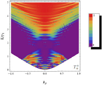
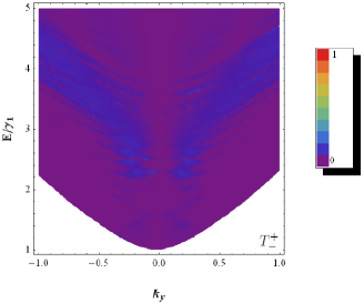
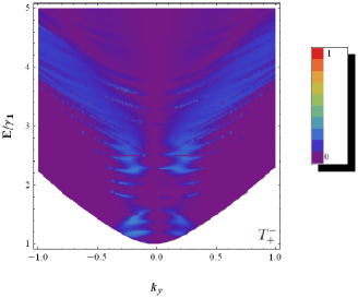
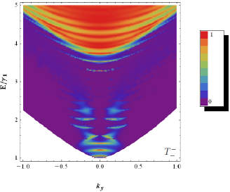
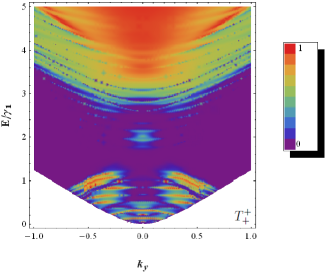
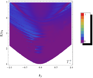
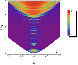
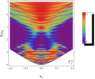
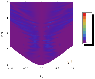
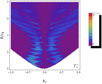
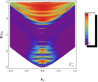
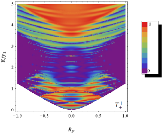
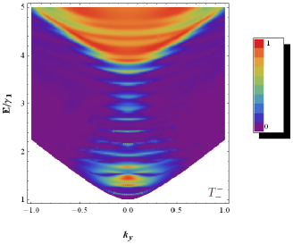
For energies larger than the interlayer coupling, $E>\gamma_{1}$, we will have four transmission channels resulting in what we call the four band tunneling. Therefore, in the transmission channels $T_{+}^{+}$ and $T_{-}^{-}$ electrons propagate via $\alpha^{+}$ and $\alpha^{-}$ mode, respectively. For $T_{-}^{+}$ scattering from $\alpha^{+}$ mode to the $\alpha^{-}$ mode and $T_{+}^{-}$ operates in the other direction [18, 19, 20]. In Figure 3, we show the different channels associated with the four transmission probabilities as a function of the transfer wave vector $k_{y}$ and energy $E$. The potential barrier heights are set to be $V_{2}=V_{4}=2.5\ \gamma_{1}$, $V_{3}=1.5\ \gamma_{1}$ and the interlayer potential difference is zero, i.e. $\delta_{2}=\delta_{3}=\delta_{4}=0\ \gamma_{1}$. For energies smaller than $V_{3}-\gamma_{1}$, there are propagating $\alpha^{+}$ states in the region $j=3$, which lead to a nonzero transmission in the $T_{+}^{+}$ channel. The cloak effect [24] occurs in the energy region $V_{3}-\gamma_{1}<E<V_{3}$ for nearly normal incidence, in $T_{+}^{+}$ channel $\left(k_{y}\approx-\frac{d_{3}}{l_{B}^{2}}\ \mbox{and}\ k_{y}\approx-\frac{d_{2}}{l_{B}^{2}}\right)$, in $T_{-}^{+}$ channel $\left(k_{y}\approx-\frac{d_{3}}{l_{B}^{2}}\right)$ and in $T_{+}^{-}$ channel $\left(k_{y}\approx-\frac{d_{2}}{l_{B}^{2}}\right)$ where the two modes $\alpha^{+}$ and $\alpha^{-}$ are decoupled and therefore no scattering occurs between them [18, 19]. While for non-normal incidence the two modes $\alpha^{+}$ and $\alpha^{-}$ are coupled, so that the transmissions $T_{+}^{+}$, $T_{-}^{+}$ and $T_{+}^{-}$ channels are not zero. The transmission probabilities $T_{-}^{+}$ and $T_{+}^{-}$ are different ($T_{-}^{+}\neq T_{+}^{-}$), which introduces the asymmetry of double barrier in the presence of a magnetic field and $V_{3}\neq 0$. In fact, these transmission probabilities are associated with electrons moving in opposite direction. For $T_{-}^{-}$ electrons propagate via $\alpha^{-}$ mode in the two energy regimes $E<V_{3}$ and $E>V_{2}+\gamma_{1}$, but is absent in the energy regime $V_{2}<E<V_{2}+\gamma_{1}$ so that the transmission is suppressed in this region, which is equivalent to the cloak effect [18, 19, 20]. Additionally, in the four transmission channels the resonances are resulting from the bound electrons in the well between the two barriers ($V_{3}<E<V_{2}=V_{4}$).

Figure 3: Density plot of the four transmission channels as a function of the transverse wave vector $k_{y}$ and its energy $E$, with $V_{2}=V_{4}=2.5\ \gamma_{1}$, $V_{3}=1.5\ \gamma_{1}$, $\delta_{2}=\delta_{3}=\delta_{4}=0\ \gamma_{1}$, $l_{B}=18.5\ nm$, $d_{4}=-d_{1}=14\ nm$ and $d_{3}=-d_{2}=7.5\ nm$.

Now let see how the interlayer potential difference will affect the different transmission channels. In Figure 4, we present the density plot of the four transmission channels as function of the transfer wave vector $k_{y}$ and energy $E$. We consider the same parameters as in Figure 3 but for $\delta_{2}=\delta_{4}=0.4\ \gamma_{1}$ and $\delta_{3}=0.2\ \gamma_{1}$. We notice that the four transmission channels are related to the transmission gap around to the Dirac points $E=V_{2}=V_{4}$ and $E=V_{3}$. It is clearly seen that the transmission display sharp peaks inside the transmission gap around the Dirac point $E=V_{2}=V_{4}$. These peaks can be attributed to the bound states formed in the double barrier structure [19]. That are correlated to the transmission gap and show a suppression due to cloak effect around $E=V_{3}$, as it was the case for the single barrier [20].

Figure 4: Density plot of the four transmission channels as a function of the transverse wave vector $k_{y}$ and its energy $E$, with $V_{2}=V_{4}=2.5\ \gamma_{1}$, $V_{3}=1.5\ \gamma_{1}$, $\delta_{2}=\delta_{4}=0.4\ \gamma_{1}$, $\delta_{3}=0.2\ \gamma_{1}$, $l_{B}=18.5\ nm$, $d_{4}=-d_{1}=14\ nm$ and $d_{3}=-d_{2}=7.5\ nm$.

Figure 5: Density plot of the four transmission channels as a function of the transverse wave vector $k_{y}$ and its energy $E$, with $V_{2}=V_{4}=2.5\ \gamma_{1}$, $V_{3}=0\ \gamma_{1}$, $\delta_{2}=\delta_{3}=\delta_{4}=0\ \gamma_{1}$, $l_{B}=18.5\ nm$, $d_{4}=-d_{1}=14\ nm$ and $d_{3}=-d_{2}=7.5\ nm$.

Figure 6: Density plot of the four transmission channels as a function of the transverse wave vector $k_{y}$ and its energy $E$, with $V_{2}=V_{4}=2.5\ \gamma_{1}$, $V_{3}=0\ \gamma_{1}$, $\delta_{2}=\delta_{4}=0.4\ \gamma_{1}$, $\delta_{3}=0.\ \gamma_{1}$, $l_{B}=18.5\ nm$, $d_{4}=-d_{1}=14\ nm$ and $d_{3}=-d_{2}=7.5\ nm$.

In Figure 5 we show the different channels associated with the four transmissions as a function of the transverse wave vector $k_{y}$ and energy $E$. The height of the potential is set to $V_{2}=V_{4}=2.5\ \gamma_{1}$ and $V_{3}=0\ \gamma_{1}$. We notice that the Dirac fermions exhibit transmission resonance in $T_{+}^{+}$ channel in the region $E<V_{2}-\gamma_{1}$ where the electrons propagate via $\alpha^{+}$. The cloak effect [24] appears in the region $V_{2}-\gamma_{1}<E<V_{2}$ for nearly normal incidence in the $T_{+}^{+}$, $T_{-}^{+}$ and $T_{+}^{-}$ channels, while for non-normal incidence it does not appear [18, 19, 20]. Introducing asymmetric double barrier structure in the presence of the magnetic field will break this equivalence such that $T_{-}^{+}\neq T_{+}^{-}$. In the four transmission channels in the energy regime $E>V_{2}=V_{4}$ they are similar to those obtained in Figure 3. In the presence of the magnetic field and for the energy regime $E<V_{2}=V_{4}$, the resonances result from the bound electrons. In addition, the resonant peaks in the regime of energy $E<V_{2}=V_{4}$ are more intense compared to those obtained in Figure 3. For $T_{-}^{-}$ electrons propagate via $\alpha^{-}$ mode which is absent between the two barriers ($E<V_{2}=V_{4}$) so that the transmission is suppressed in this region and this is equivalent to the cloak effect [24].

Now let us investigate the effect of the interlayer potential difference on the band structure. We show the four channels of the transmission probabilities in Figure 6. For the same parameters as in Figure 5 but for an interlayer potential difference $\delta_{2}=\delta_{4}=0.4\ \gamma_{1}$ and $\delta_{3}=0\ \gamma_{1}$. The general behavior of these different channels resembles the single barrier case in the presence of a magnetic fields [20], with some major differences such as the observation of peaks in the region $V_{2}-\delta_{2}<E<V_{2}+\delta_{2}$. These peaks are due to the existence of bounded states [19].

5 Conclusion

In summary, we evaluated the transmission probabilities in AB-stacked bilayer graphene through a double barrier potential in the presence of a uniform magnetic field. We formulated our model Hamiltonian that describes the system and computed the associated energy eigenvalues as well as the band structure. We obtained a full four bands of the energy spectrum and solved for the spinor solution in each region of our system. The boundary conditions were used to calculate the transmission probabilities which were computed numerically.

We found that the transmission can be enhanced due to the presence of two propagation modes whose energy scale is set by the interlayer coupling. For energies less than the height of the barrier the Dirac fermions exhibit transmission resonances and only one propagation mode is available. The transmission at nearly normal incidence is zero and does not show any resonances in the regime of energy $E<V_{3}$. Resonances are present for non-normal incidence, this is equivalent to the situation of a single barrier. In addition, the presence of the peaks in the regime of energy $V_{3}<E<V_{2}=V_{4}$ are due to the bound electron states. However, these peaks are absent in the case of a single barrier. When the energy is higher than the interlayer coupling two propagation modes are available for transport giving rise to four possible ways for transmission probabilities.

We also found that for the case with $V_{3}\neq 0$ resonant peaks are more intense compared to those obtained for $V_{3}=0$. Then, we studied how the interlayer potential difference affects the transmission probability. We found that the transmission displays sharp peaks inside the transmission gap (around the Dirac point $E=V_{2}=V_{4}$), that are absent around $E=V_{3}$. These peaks can be attributed to the bound states formed by the double barrier potential.

References

• [1] A. K. Geim and K.S. Novoselov, Nature Materials 6, 183 (2007).
• [2] K. S. Novoselov, A. K. Geim, S. V. Morozov, D. Jiang, M. I. Katsnelson, I. V. Grigorieva, S. V. Dubonos and A. A. Firsov, Nature 438, 197 (2005).
• [3] Y. B. Zhang, Y. W. Tan, H. L. Stormer and P. Kim, Nature 438, 201 (2005).
• [4] S. V. Morozov, K. S. Novoselov, M. I. Katsnelson, F. Schedin, D. C. Elias, J. A. Jaszczak and A. K. Geim, Physical Review Letters 100, 016602 (2008).
• [5] Y. M. Lin, C. Dimitrakopoulos, K. A. Jenkins, D. B. Farmer, H. Y. Chiu, A. Grill and P. Avouris, Science 327, 662 (2010).
• [6] A. H. Castro Neto, F. Guinea, N. M. R. Peres, K. S. Novoselov and A. K. Geim, Reviews of Modern Physics 81, 109 (2009).
• [7] E. McCann and V. I. Fałko, Physical Review Letters 96, 086805 (2006).
• [8] K. S. Novoselov, E. McCann, S. V. Morozov, V. I. Fałko, M. I. Katsnelson, U. Zeitler, D. Jiang, F. Schedin and A. Geim, Nature Physics 2, 177 (2006).
• [9] K. S. Novoselov, V. I. Fałko, L. Colombo, P. R. Gellert, M. G. Schwab and K. Kim, Nature 490, 192 (2012).
• [10] S. Y. Zhou, D. A. Siegel, A. V. Fedorov, F. El Gabaly, A. K. Schmid, A. H. Castro Neto and A. Lanzara, Nature Materials 7, 259 (2007).
• [11] R. Costa Filho, G. Farias and F. Peeters, Physical Review B 76, 193409 (2007).
• [12] Y. Zhang, T.-T. Tang, C. Girit, Z. Hao, M.C. Martin, A. Zettl, M.F. Crommie, Y.R. Shen and F. Wang, Nature 459, 820 (2009).
• [13] E. McCann, Physical Review B 74, 1 (2006).
• [14] F. Guinea , A. H. C. Neto and N. M. R. Peres, Physical Review B 73, 245426 (2006).
• [15] S. Latil and L. Henrard, Physical Review Letters 97, 036803 (2006).
• [16] B. Partoens and F. M. Peeters, Physical Review B 74, 075404 (2006).
• [17] M. I. Katsnelson, K. S. Novoselov and A. K. Geim, Nature Physics 2, 620 (2006).
• [18] B. V. Duppen and F.M. Peeters, Physical Review B 87, 205427 (2013).
• [19] H. A. Alshehab, H. Bahlouli, A. El Mouhafid and A. Jellal, arXiv: 1401.5427 (2014).
• [20] A. Jellal, I. Redouani and H. Bahlouli, Physica E 72, 149 (2015)
• [21] P. R. Wallace, Physical Review 71, 622 (1947); J. C. Slonczewski and P. R. Weiss, Physical Review 109, 272 (1958).
• [22] J. W. McClure, Physical Review 108, 612 (1957).
• [23] I. Snyman and C. W. J. Beenakker, Physical Review B 75, 045322 (2007).
• [24] N. Gu, M. Rudner and L. Levitov, Physical Review Letters 107, 156603 (2011).