Radially anisotropic systems with $r^{-\alpha}$ forces: equilibrium states

Abstract

We continue the study of collisionless systems governed by additive $r^{-\alpha}$ interparticle forces by focusing on the influence of the force exponent $\alpha$ on radial orbital anisotropy. In this preparatory work we construct the radially anisotropic Osipkov-Merritt phase-space distribution functions for self-consistent spherical Hernquist models with $r^{-\alpha}$ forces and $1\leq\alpha<3$. The resulting systems are isotropic at the center and increasingly dominated by radial orbits at radii larger than the anisotropy radius $r_{a}$. For radially anisotropic models we determine the minimum value of the anisotropy radius $r_{ac}$ as a function of $\alpha$ for phase-space consistency (such that the phase-space distribution function is nowhere negative for $r_{a}\geq r_{ac}$). We find that $r_{ac}$ decreases for decreasing $\alpha$, and that the amount of kinetic energy that can be stored in the radial direction relative to that stored in the tangential directions for marginally consistent models increases for decreasing $\alpha$. In particular, we find that isotropic systems are consistent in the explored range of $\alpha$. By means of direct $N$-body simulations we finally verify that the isotropic systems are also stable.

1 Introduction

It is well known that spherically symmetric, self-gravitating collisionless equilibrium systems in which a significant fraction of the kinetic energy is stored in low angular momentum orbits are dynamically unstable. The associated instability is known as Radial Orbit Instability (hereafter ROI, see e.g. Fridman & Polyachenko 1984; 2014, 2008; for a recent discussion see also Polyachenko & Shukhman 2015 and references therein). Usually, the amount of radial anisotropy in a spherical system is quantified by introducing the Fridman-Polyachenko-Shukhman parameter

$$\xi\equiv\frac{2K_{r}}{K_{t}},$$ (1)

where the radial and tangential kinetic energies are given respectively by

$$K_{r}=2\pi\int\rho(r)\sigma^{2}_{r}(r)r^{2}{\rm d}r,\quad K_{t}=2\pi\int\rho(r)\sigma^{2}_{t}(r)r^{2}{\rm d}r.$$ (2)

In the expressions above $\rho$ is the system density, and $\sigma^{2}_{r}$ and $\sigma^{2}_{t}$ are the radial and tangential phase-space averaged square velocity components (see Polyachenko & Shukhman, 1981; Polyachenko, 1992): in particular, for isotropic systems $\xi=1$. In the case of Newtonian force numerical simulations show that the ROI typically occurs for $\xi\gtrsim 1.7$, but this should be considered a fiducial value, as it is also well known that the critical value of $\xi$ above which the given system is unstable depends on the specific phase-space structure of the equilibrium configuration under study (see, e.g. Merritt & Aguilar, 1985; , 1989; Saha, 1991; , 1994; Meza & Zamorano, 1997; , 2002, 2009).
Due to its relevant astrophysical consequences, and its intrinsic physical interest for the understanding of collisionless systems, the ROI has been extensively studied in Newtonian gravity (see e.g. Palmer & Papaloizou, 1987; , 2015, and references therein). For example, (2002) investigated the implications of the ROI for the Fundamental Plane of elliptical galaxies, excluding the possibility that the so-called tilt of the Fundamental Plane is just due to a systematic increase of radial orbits with galaxy mass (see also Ciotti 1997, Ciotti & Lanzoni 1997). In a different context (Ciotti & Pellegrini 2004) it has been shown that the constraints on the maximum amount of radial anisotropy that can be sustained by a stable stellar system can be used to dismiss some models of mass distribution in elliptical galaxies that have been obtained by using X-ray data under the assumption of hydrostatic equilibrium of the hot interstellar medium. The ROI also plays a role in the course of Violent Relaxation (1967), i.e., the collapse and virialization of cold self-gravitating systems (e.g. see , 1982, 1991, 2006), because such collapses are dominated in their last stages by significant radial motions, and so ROI contributes to establish the dynamical and structural properties of the quasi-relaxed final states (e.g. Merritt & Aguilar 1985; 2005, 2015).
From a more general point of view, it is now known that the ROI is not a specific property of Newtonian gravity. For example (2011) have studied the ROI in Modified Newtonian Dynamics (hereafter MOND; 1983; 1984), comparing anisotropic MOND systems with their Equivalent Newtonian Systems with dark matter, (i.e., systems in which the phase-space properties and total gravitational potential are the same as in the corresponding MOND systems). Numerical simulations showed that MOND systems are more prone to develop ROI than their ENSs. At the same time, MOND systems are able to support a larger amount of kinetic energy stored in radial orbits than one-component Newtonian systems with the same density distribution.
Some natural questions then arise. What is the dependence of the ROI on the specific force law? How much the long- or short-range nature of the interparticle force influences the ROI? Are there any aspects of the ROI that are peculiar of the Newtonian force (which stands out among power-law forces for several unique mathematical properties)? In fact, though several features of the dynamical evolution of collisionless systems have found to be quite independent of the specific force law, some other aspects show a clear dependence on it. For example, in the low-acceleration regime, collisionless relaxation is much less efficient in MOND than in Newtonian gravity (2007, 2007a, 2007b), and a similar result is found for power-law forces with $\alpha<2$ (Di Cintio & Ciotti 2011).
In particular, (2013) (see also Di Cintio & Ciotti 2011) studied by means of direct $N-$body simulations the dissipationless collapses of cold and spherical systems of particles interacting via additive interparticle $r^{-\alpha}$ forces. The main results of these works are that, almost independently of $\alpha$, the considerably radially anisotropic final states of cold collapses have surface density profiles following the Sérsic (1968) law, and differential energy distributions well described by an exponential over a large range of energies. At fixed initial virial ratio however, a non-monotonic trend of the Sérsic index $m$ (the parameter determining the shape of the density profile, see e.g. 1991, 1999) with the force index is found. Remarkably, the $\alpha=1$ case (corresponding qualitatively to the force in the deep-MOND regime), behaves very similarly to MOND, although this last theory is non-additive (the MOND field equation involves the $p$-Laplace operator).
Prompted by these findings and by the above questions, here we set the stage for the study of ROI in the case of power-law forces, by constructing a family of radially anisotropic Hernquist (1990) models with additive $r^{-\alpha}$ forces, and restricting to the range $1\leq\alpha<3$. Such interval contains the Newtonian $\alpha=2$ case, explores ”short-range” forces ($\alpha>2$) and also long-range forces ($\alpha<2$), down to the MOND-like case $\alpha=1$. Smaller values of $\alpha$ are excluded by this preparatory investigation (we recall that the $\alpha=-1$ case corresponds to the harmonic force, for which no relaxation takes place, see e.g. 1982). Power-law forces with $\alpha\geq 3$ are also excluded by the present analysis, due to their very peculiar properties (for example, self-gravitating systems with $\alpha=3$ can be virialized only for zero total energy). We notice that the study of the dynamics under the effect of power-law forces is by no means new: very important examples can be traced back to Newton’s Principia (e.g. see 1995).
This paper is structured as follows. In Section 2, we construct isotropic and radially anisotropic self gravitating spherical Hernquist models with $r^{-\alpha}$ forces, and we study their phase-space consistency and the properties of their velocity dispersion profiles. In Section 3 we presents numerical results on the stability of the isotropic systems. Section 4 summarizes.

2 Radially anisotropic equilibria

The first step for the realization of the $N-$body simulations of ROI for systems ruled by generalized power-law forces is the construction of their equilibrium phase-space distribution function $f$, in a framework allowing for tunable amount of radial anisotropy (i.e. different values of $\xi$). It is well known that the amount of radial orbits that can be imposed to a physically acceptable equilibrium stellar system is limited by phase-space consistency (i.e. by the positivity of the associated $f$): stability can be studied only for consistent systems. Therefore, before embarking in the study of the stability of a system it is fundamental to be reassured that its equilibrium initial condition actually exists. For these reasons in the next Section we proceed to construct the phase-space distribution function for the widely used Hernquist (1990) profile, under the effect of the $r^{-\alpha}$ force.

2.1 The phase-space distribution function

We begin by considering the problem of the construction of the phase-space distribution function $f$ for a generic equilibrium spherical system of given density profile $\rho(r)$, under the action of the $r^{-\alpha}$ force with $1\leq\alpha<3$. In principle, different velocity anisotropy profiles can be imposed on a given density profile. In this work, in order to build systems with a tunable degree of radial anisotropy, we adopt widely used Osipkov-Merritt extension of the classical Eddington (1916) inversion:

$$f(Q)=\frac{1}{\sqrt{8}\pi^{2}}\frac{\rm d}{{\rm d}Q}\int_{Q}^{Q_{\rm sup}}\frac{{\rm d}\rho_{a}}{{\rm d}\Phi}\frac{{\rm d}\Phi}{\sqrt{\Phi-Q}}=\frac{1}{\sqrt{8}\pi^{2}}\int_{Q}^{Q_{\rm sup}}\frac{{\rm d^{2}}\rho_{a}}{{\rm d}\Phi^{2}}\frac{{\rm d}\Phi}{\sqrt{\Phi-Q}},$$ (3)

where for a system of finite total mass $Q_{\rm sup}=0$ for $\alpha>1$, and $Q_{\rm sup}=\infty$ for $\alpha\leq 1$ (see the following discussion). Here $\Phi$ is the (self-consistent) gravitational potential, $Q=E+{J^{2}}/{2r_{a}^{2}}$, where $E$ and $J$ are the specific (per unit mass) particle energy and angular momentum modulus, respectively,

$$\rho_{a}(r)\equiv\left(1+\frac{r^{2}}{r_{a}^{2}}\right)\rho(r)$$ (4)

is the so-called augmented density, and $r_{a}$ is the anisotropy radius (Osipkov, 1979; Merritt, 1985). Due to the dependence of $f$ on global integrals of motion, it follows from the Jeans theorem that the equilibrium phase-space distribution function $f(Q)$ satisfies the Vlasov equation (also known as the Collisionless Boltzmann Equation, see e.g. 2008, 2014) Integration of $f(Q)$ over the velocity space after multiplication by the appropriate velocity components shows that the anisotropy profile associated with eq. (3) is

$$\beta(r)\equiv 1-\frac{\sigma_{t}^{2}(r)}{2\sigma_{r}^{2}(r)}=\frac{r^{2}}{r_{a}^{2}+r^{2}},$$ (5)

where $\sigma_{t}(r)$ and $\sigma_{r}(r)$ are the tangential and radial velocity dispersion profiles of the system (see e.g. , 2008). In practice, Osipkov-Merritt models are everywhere isotropic for ${r_{a}}\to\infty$ and become more and more radially anisotropic for decreasing values of $r_{a}$; at fixed $r_{a}$ they are isotropic for $r\ll r_{a}$ and radially anisotropic for $r\gg r_{a}$. It is easy to show that the above formulae, derived in the literature for Newtonian gravity, are independent of the specific force law adopted.

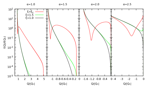
Figure 1: Phase-space distribution functions for Osipkov-Merritt radially anisotropic Hernquist models with $\alpha=1$, 1.5, 2 and 2.5. The normalization constant is $Q_{*}=\Phi(r_{*})$, where $r_{*}$ is the half-mass radius. The black curves correspond to the isotropic case ($\xi=1$), while the green ones to $\xi=1.5$, the fiducial value for the onset of ROI in Newtonian ($\alpha=2$) systems. The red curves show $f(Q)$ for values of $\xi$ near the consistency limit $\xi_{c}=\xi(r_{ac})$ (see Sect. 2.2).

From eq. (3) it follows that the first step needed to recover $f$ is the knowledge of the self consistent potential $\Phi$ of the system. For a generic density $\rho(\mathbf{x})$ the $\alpha-$potential can be written as

$$\Phi(\mathbf{x})-\Phi(\mathbf{x}_{0})=-\frac{G}{\alpha-1}\int_{\mathbb{R}^{3}}\left(\frac{1}{||\mathbf{x}-\mathbf{y}||^{\alpha-1}}-\frac{1}{||\mathbf{x}_{0}-\mathbf{y}||^{\alpha-1}}\right)\rho(\mathbf{y}){\rm d}^{3}\mathbf{y}$$ (6)

for $\alpha\neq 1$, and as

$$\Phi(\mathbf{x})-\Phi(\mathbf{x}_{0})=G\int_{\mathbb{R}^{3}}\ln\frac{||\mathbf{x}-\mathbf{y}||}{||\mathbf{x}_{0}-\mathbf{y}||}\rho(\mathbf{y}){\rm d}^{3}\mathbf{y}$$ (7)

for $\alpha=1$. In the equations above $G$ is a dimensional coupling constant and $\mathbf{x}_{0}$ is a reference point to be chosen from convergence considerations. The value of $\Phi(\mathbf{x}_{0})$ is usually fixed by arguments of convenience as illustrated below. Note that, when convergence is assured, eq. (7) follows from (6) for $\alpha\to 1$, provided that $||\mathbf{x}_{0}||<\infty$.
Elementary integration shows that for a spherical density distribution $\rho(r)$ of finite mass, the potential can be written for $1<\alpha<3$ as

$$\Phi(r)=-\frac{2\pi G}{r}\int_{0}^{\infty}\frac{(r+r^{\prime})^{3-\alpha}-|r-r^{\prime}|^{3-\alpha}}{(\alpha-1)(3-\alpha)}r^{\prime}\rho(r^{\prime}){\rm d}r^{\prime},$$ (8)

having set to zero the value of the potential for $r\to\infty$, and assumed $||\mathbf{x}_{0}||\to\infty$. For $\alpha=1$ some care is needed in order to define $\Phi(r)$, and it can be shown that for a system of finite mass the potential can be written as

$$\Phi(r)=\frac{\pi G}{r}\int_{0}^{\infty}\left[(r+r^{\prime})^{2}\ln\frac{r+r^{\prime}}{r_{n}}-(r-r^{\prime})^{2}\ln\frac{|r-r^{\prime}|}{r_{n}}-2rr^{\prime}\right]r^{\prime}\rho(r^{\prime}){\rm d}r^{\prime},$$ (9)

where now $\mathbf{x}_{0}=0$, and $r_{n}$ is an arbitrary normalization length: different choices of $r_{n}$ just correspond to a different additive constant in the value of $\Phi$. As expected eqs. (8) and (9) are more complicated than their Newtonian counterparts, because Newton’s theorems do not hold for $\alpha\neq 2$. However, in general the potential at large radii for $1<\alpha<3$ is dominated by the very simple asymptotic monopole term

$$\Phi(r)\sim-\frac{GM}{(\alpha-1)r^{\alpha-1}},$$ (10)

while in the $\alpha=1$ case the monopole term for $r\to\infty$ diverges as

$$\Phi(r)\sim GM\ln\frac{r}{r_{n}}.$$ (11)

Note that, the expansions in eqs. (10) and (11) hold true also in the case of non-spherical density profiles, as can be seen from eqs. (6) and (7) for systems of finite total mass.
In the present work we focus on systems described by the Hernquist (1990) density distribution

$$\rho(r)=\frac{M}{2\pi r_{c}^{2}r(1+r/r_{c})^{3}},$$ (12)

where $M$ is the total mass, $r_{c}$ is the core radius and $r_{*}=(1+\sqrt{2})r_{c}$ is the half-mass radius, i.e. the radius of the sphere enclosing half of the total mass.
For the distribution (12) and $1<\alpha<3$ the potential at the centre can be evaluated analytically and reads

$$\Phi(0)=-\frac{GM}{r_{c}^{\alpha-1}}\frac{2{\rm B}(3-\alpha,\alpha)}{\alpha-1},$$ (13)

where ${\rm B}(x,y)$ is the Complete Euler Beta function. Curiously, the dimensionless factor in equation above is a non monotonic function of $\alpha$, with maximum -1 reached for $\alpha=2$, and diverging at $-\infty$ for $\alpha\to 1^{+}$ and $\alpha\to 3^{-}$. For $\alpha=1$ the central potential is instead finite and reads

$$\Phi(0)=GM\left(1+\ln\frac{r_{c}}{r_{n}}\right);$$ (14)

its numerical value depends on the normalization length $r_{n}$. For Hernquist models with $\alpha=1$ the natural choice is to adopt $r_{n}=r_{c}$. It is not surprising that the limit of eqs. (10) and (13) for $\alpha\to 1^{+}$ differs from eqs. (11) and (14), as two different choices of $\mathbf{x}_{0}$ have been adopted for $1<\alpha<3$ and $\alpha=1$ (see the discussion after eq. 7). In general, the (1853) theorem on the integration of differential binomials assures that the integral in eq. (8) can be evaluated in terms of elementary functions for the Hernquist model for all rational values of $\alpha$. However, the formulae are cumbersome, so we computed eqs. (8) and (9) numerically; as a safety check we verified that the numerical results reproduce the asymptotic expansions at large radii (equations 10 and 11) as well as the values of $\Phi(0)$.

2.2 Consistency

In Newtonian gravity $(\alpha=2)$ anisotropic Osipkov-Merritt systems of given $\rho(r)$ are characterized by a critical value of the anisotropy radius, $r_{ac}$, such that for $r_{a}<r_{ac}$ the corresponding models are inconsistent (Ciotti & Pellegrini 1992, see also 1995; Ciotti 1996, 1999; 2010a, b, 2012). It is therefore important for our study to determine the minimum value $r_{ac}(\alpha)$ associated with a nowhere negative (i.e. consistent) $f(Q)$. From eq. (3) it follows that the phase-space distribution function of an Osipkov-Merritt model (independently of the force law) can be written as

$$f(Q)=f_{i}(Q)+\frac{f_{a}(Q)}{r_{a}^{2}},$$ (15)

where $f_{i}$ is the phase-space distribution function in the isotropic case ($r_{a}\to\infty$). For the Hernquist density profile we found that $f_{i}\geq 0$ for all the explored values of $\alpha$ i.e. the isotropic Hernquist model is consistent under $r^{-\alpha}$ forces, as already known for the Newtonian case.

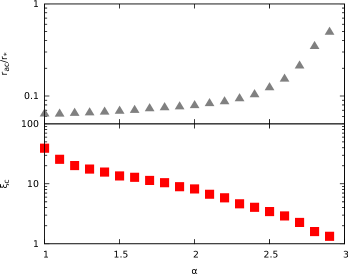
Figure 2: Minimum value $r_{ac}$ of the anisotropy radius for phase-space consistency (in units of the half-mass radius $r_{*}$) of the Hernquist model with Osipkov-Merritt radial anisotropy and the corresponding value of the Fridman-Polyachenko-Shukhman index $\xi_{c}=\xi(r_{ac})$, as functions of the force exponent $\alpha$.

Being this assured, then the critical anisotropy radius is given by

$$r_{ac}^{2}={\rm sup}\left[-\frac{f_{a}(Q)}{f_{i}(Q)}\right],\quad Q\in A^{-},$$ (16)

where the sup in the r.h.s. is evaluated over the region $A^{-}$ of $Q$ values corresponding to $f_{a}<0$ (see Ciotti, 2000).
The numerically recovered phase-space distribution functions for $\alpha=1,$ 1.5, 2 and 2.5 and different values of $r_{a}$ (with the corresponding values of $\xi$) are presented in Fig. 1. Of course, $\Phi(0)\leq Q<0$ for $1<\alpha<3$, and $\Phi(0)\leq Q\leq\infty$ for $\alpha=1$. For $\xi\simeq\xi_{c}$, i.e. $r_{a}\simeq r_{ac}$ (red curves), $f(Q)$ shows a strong non-monotonicity, due to the almost dominant negative contribution of $f_{a}/r_{a}^{2}$ over the isotropic and positive $f_{i}$. A further reduction of $r_{a}$ would deepen even more the depression in the red curves, finally leading to a negative $f$, and to phase-space inconsistency. The relation of monotonicity of $f(Q)$ and ROI is a very important point that at this stage we cannot address, but that will be central in our forthcoming study (for example by considering the possibility to extend the Antonov laws to $r^{-\alpha}$ forces; see 2008).
In Fig. 2 we show for $1\leq\alpha<3$ the values of $r_{ac}$, and their associated $\xi_{c}=\xi(r_{ac})$. In the Newtonian case ($\alpha=2$) $r_{ac}/r_{*}\simeq 0.08$, in accordance with analytic results (Ciotti 1996). From Fig. 2 it is also apparent that systems with lower values of $\alpha$ (i.e. forces with a longer range than Newtonian) can sustain smaller values of the anisotropy radius (associated with larger values of $\xi_{c}$) implying that they are able to store a larger fraction of the kinetic energy in low-angular momentum orbits maintaining a nowhere negative phase-space distribution function.

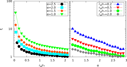
Figure 3: Fridman-Polyachenko-Shukhman parameter $\xi$ as a function of the normalized anisotropy radius $r_{a}/r_{*}$, and of the force exponent $\alpha$, for Osipkov-Merritt radially anisotropic Hernquist models with $r^{-\alpha}$ forces.

Figure 3 (left panel) shows the parameter $\xi$ as a function of the anisotropy radius $r_{a}$ for $\alpha=1,$ 1.5, 2 and 2.5. As expected, $\xi$ decreases monotonically for increasing $r_{a}$ for all values of $\alpha$. A complementary illustration of this behaviour is given in the right panel, where the trend of $\xi$ with $\alpha$ for a selection of values of $r_{a}$ is given.
A more detailed representation of the effects of $\alpha$ and $r_{a}$ on the internal dynamics of the models can be obtained by plotting the velocity dispersion profiles. The radial velocity dispersion $\sigma_{r}$ is given by the Jeans equation

$$\frac{{\rm d}\rho\sigma_{r}^{2}}{{\rm d}r}+\frac{2\beta\rho\sigma_{r}^{2}}{r}=-\rho\frac{{\rm d}\Phi}{{\rm d}r},$$ (17)

whose solution in case of Osipkov-Merritt anisotropic systems is

$$\rho(r)\sigma_{r}^{2}(r)=\frac{\int_{r}^{\infty}\rho(r^{\prime})(r^{\prime 2}+r_{a}^{2})\frac{{\rm d}\Phi}{{\rm d}r^{\prime}}dr^{\prime}}{r^{2}+r_{a}^{2}}.$$ (18)

It is easy to show that, for a density profile decreasing at large radii as $r^{-\lambda}$ with $\lambda>3$, and in presence of $r^{-\alpha}$ forces,

$$\sigma_{r}^{2}(r)\simeq\frac{GM}{r^{2}+r_{a}^{2}}\left(\frac{r^{3-\alpha}}{\alpha+\lambda-3}+\frac{r_{a}^{2}r^{1-\alpha}}{\alpha+\lambda-1}\right).$$ (19)

In particular, for $\alpha=1$, in the limit $r\rightarrow\infty$, $\sigma_{r}^{2}$ flattens to the constant value $GM/(\lambda-2)$ due to the logarithmic nature of the potential for a system of finite mass (see eq. 11). Specifically, for the Hernquist density profile given by eq. (12), $\lambda=4$, and thus $\sigma_{r}\simeq\sqrt{GM/2}$ at large radii. In Fig. 4 we present the radial and tangential velocity dispersion profiles $\sigma_{r}(r)$ and $\sigma_{t}(r)$ for $r_{a}/r_{*}=0.5,$ 1 and 2, obtained by numerically solving eq. (18). As a further test of the numerical recovery of $f(Q)$ we verified that the profiles of $\sigma_{r}$ and $\sigma_{t}$ extracted from $N-$body realizations obtained by sampling the numerically evaluated $f(Q)$ reproduce the curves shown in Fig. 4. It is apparent how for increasing $\alpha$, independently of $r_{a}$ the components of the velocity dispersion become more and more peaked at inner radii. As expected, for the MOND-like ($\alpha=1$) case, the radial profile of $\sigma_{r}$ is always flat for all the explored values of $r_{a}$, in agreement with eq. (19) and with the numerical results of (2013). Once the profiles of $\sigma_{r}^{2}$ and $\sigma_{t}^{2}$ are known (see eq. 5), it is immediate to evaluate $K_{r}$ and $K_{t}$ by numerical integration. In particular, the relatively flat profiles of $\sigma_{r}$ at large radii for small values of $\alpha$ are at the origin of the high values of $\xi$ with respect to those obtained for larger values of $\alpha$. The behaviour of $\xi$ as a function of $r_{a}$ and $\alpha$ can be also easily illustrated with the aid of a very simple toy model. In practice, one can integrate eq. (19) for a constant density ”atmosphere”, $\rho(r)=\rho_{0}$ for $r\leq R$, under the gravitational field of a central point mass, $-GM/r^{\alpha}$. The radial velocity dispersion profile is of elementary evaluation, while $K_{r}$ in general is given by hypergeometric (Euler Beta) functions. However, again from the Chebyshev theorem, $K_{r}$ can be expressed in terms of elementary functions for all rational values of $\alpha$. $K_{t}$ is then obtained from the Virial theorem as $K_{t}=-K_{r}+|W|/2$ where $W$ is given in the following eq. (21), which for the toy model here considered gives $W=-4\pi G\rho_{0}MR^{4-\alpha}/(4-\alpha)$.

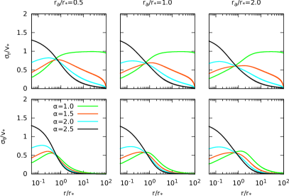
Figure 4: Radial and tangential velocity dispersion profiles of the self-consistent radially anisotropic Hernquist model with $r^{-\alpha}$ forces, for $r_{a}/r_{*}=0.5$, 1 and 2; $r_{*}$ is the half-mass radius of the distribution. The velocity dispersions are expressed in units of $v_{*}=r_{*}/t_{*}$, and $t_{*}$ is given in eq. (20). The flat outer parts of the green curve ($\alpha=1$) in the top panels are in excellent agreement with the expected value from eq. (19), and $\lambda=4$.

3 Stability of isotropic systems

As a first sample of the numerical simulations that will be performed in a forthcoming work, we present here direct $N-$body simulations aimed at testing the stability of isotropic ($\xi=1$) Hernquist models for various values of $\alpha$. The initial conditions are generated as in (2002) with a Monte Carlo sampling of $f(Q)$. The equations of motion for $N=25000$ equal-mass particles are integrated with a second order symplectic scheme with fixed timestep $\Delta t=t_{*}/100$, where the natural dynamical time-scale is defined as

$$t_{*}\equiv\sqrt{\frac{2r_{*}^{\alpha+1}}{GM}}$$ (20)

(see Di Cintio & Ciotti 2011 and 2013). In the code, the divergence of force and potential at vanishing inter-particle separation is cured with the introduction of a softening length $\epsilon$, so that in practice the potential due to each particle is smoothed as $\Phi\propto 1/(r^{2}+\epsilon^{2})^{(\alpha-1)/2}$ for $\alpha>1$, and $\Phi\propto\ln(\sqrt{r^{2}+\epsilon^{2}})$ for $\alpha=1$. The optimal $\epsilon$ (in units of $r_{*}$) is fixed so that the softened force on a particle placed at $\simeq 5r_{*}$ from the centre of mass of the system differs less than $0.01\%$ from the unsoftened force. Therefore the softening length $\epsilon$ is different for different $\alpha$: $\epsilon=0.05,$ 0.07, 0.1 and 0.125 for $\alpha=1$, 1.5, 2 and 2.5 respectively.
The absence of the analogue of the Poisson equation for $r^{-\alpha}$ forces and $\alpha\neq 2$, points at direct $N-$body simulations as the most natural approach for numerical studies. However, it is also important to note the well known property that potentials associated with the $r^{-\alpha}$ force can be expanded in terms of Gegenbauer polynomials for $\alpha\neq 1$, and of Chebyshev polynomials for $\alpha=1$ (Arfken & Weber 2005), thus opening the way to the construction of tree-codes (see e.g., 2005).
In the upper panel of Fig. 5 we show, for some representative value of $\alpha$, the time evolution of the minimum-to-maximum semiaxis ratio $c/a$ of the systems. The semiaxes are defined from the eigenvalues $I_{1}\geq I_{2}\geq I_{3}$ of the tensor $I_{ij}=\sum_{k}r_{i}^{(k)}r_{j}^{(k)}$ calculated within the radius containing 0.85% of the total mass $M$ (Meza & Zamorano 1997; 2002). In the lower panel of the same figure we also show the

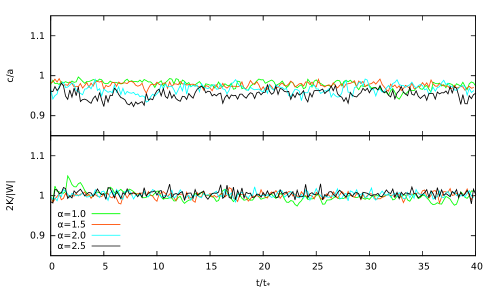
Figure 5: Evolution of the fiducial axial ratio $c/a$ and the virial ratio $2K/|W|$ for $N-$body simulations of isotropic Hernquist models with $r^{-\alpha}$ forces, and $\alpha=1$, 1.5, 2, 2.5.

time evolution of the corresponding virial ratio $2K/|W|$, where $K$ is the total kinetic energy and

$$W=-\int\rho(\mathbf{x})\langle\mathbf{x},\nabla\Phi\rangle d^{3}\mathbf{x}=\sum_{j\neq i=1}^{N}m_{i}\langle\mathbf{x}_{i},\mathbf{a}_{ji}\rangle$$ (21)

is the virial function. The second expression holds for a discrete system of particles with masses $m_{i}$, where

$$\mathbf{a}_{ji}=-Gm_{j}\frac{\mathbf{x}_{i}-\mathbf{x}_{j}}{||\mathbf{x}_{i}-\mathbf{x}_{j}||^{\alpha+1}}$$ (22)

is the acceleration on particle $i$ due to particle $j$. We recall that for $\alpha\neq 1$ $W$ is related to the system total potential energy $U$ by the identity

$$W=(\alpha-1)U,$$ (23)

where

$$U=\frac{1}{2}\int\rho(\mathbf{x})\Phi(\mathbf{x})d^{3}\mathbf{x}=\frac{1}{2}\sum_{i\neq j=1}^{N}m_{i}\Phi_{ji},$$ (24)

and in the case of a discrete system $\Phi_{ji}$ is the potential on particle $i$ due to particle $j$. For the $\alpha=1$ case (as for systems in deep-MOND regime) the virial function is independent of time, being:

$$W=-\frac{GM^{2}}{2}$$ (25)

for a continuous system, and

$$W=-\frac{G}{2}\sum_{i\neq j=1}^{n}m_{i}m_{j}$$ (26)

for a discrete system (see 2013).
From Fig. 5 it is apparent that the spherical symmetry as well as the equilibrium of the initial conditions is preserved for all the considered values of $\alpha$ up to $t/t_{*}=40$, when the simulations end.

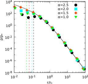
Figure 6: Final ($t/t_{*}=40$) density profiles of the same systems as in Fig. 5. Here $\rho_{*}=\rho(r_{*})$. The black solid line is the initial density profile given by eq. (12). The vertical dashed lines indicate the softening length $\epsilon$ used in the simulations.

The fluctuations are of the order of $\simeq 5\%$ in $c/a$ and $\simeq 1\%$ in $2K/|W|$. The stability of the isotropic systems is confirmed also by Fig. 6 where we compare the final density profile with the initial profile given by eq. (12). The initial density profile is preserved down to $r/r_{*}\simeq 0.025$ in the best case ($\alpha=1.5$) and to $r/r_{*}\simeq 0.8$ in the worst case ($\alpha=2.5$). In all cases the final density profiles are indistinguishable from the initial profiles for $r\gtrsim 1.4\epsilon$. In the forthcoming study we will perform a quantitative monitoring of the deterioration of the central profile as a function of $\alpha,\epsilon$ and $N$, by considering the time evolution of the Lagrangian radii containing a fixed fraction of the total mass.

4 Discussion and conclusions

In this preparatory exploration of the ROI in spherically symmetric collisionless equilibrium systems with $r^{-\alpha}$ forces we limited ourselves to a first important step, i.e. the construction of Osipkov-Merritt radially anisotropic self-consistent equilibrium models. We have recovered the potential generated by the Hernquist density distribution under $r^{-\alpha}$ forces and we have calculated the corresponding phase-space distribution functions for isotropic and anisotropic Osipkov-Merritt models in the range of values $1\leq\alpha<3$. We numerically determined, as a function of $\alpha$, the minimum value of the anisotropy radius for consistency $r_{ac}$ and the associated critical value of the Fridman-Polyachenko-Shukhman index $\xi_{c}$, and we computed the radial and tangential velocity dispersion profiles for a few representative consistent systems. The main results of this paper can be summarized as follows:

1. For $1\leq\alpha<3$ the distribution functions of the isotropic $r^{-\alpha}$ Hernquist models are monotonically decreasing and everywhere positive. Their $N-$body realizations are numerically stable up to $\simeq 40t_{*}$.

2. For anisotropic Hernquist models the minimum value of the anisotropy radius for consistency $r_{ac}$ increases with increasing $\alpha$, and the corresponding $\xi_{c}$ decreases. Therefore, systems with lower $\alpha$ can be generated with a higher amount of radial anisotropy. This appears to be in agreement with the results of (2013), who find increasingly anisotropic end products of dissipationelss collapses, when reducing $\alpha$ from 3 to 1.

3. As general trend, for all values of $\alpha$ the Fridman-Polyachenko-Shukhman index $\xi$ decreases for increasing $r_{a}$, and increases with decreasing $\alpha$ at fixed $r_{a}$.
   

In the natural follow-up of this preparatory work we will determine, as a function of $\alpha$, the critical $\xi$ for the onset of ROI, in order to understand how much this process depends on the short or long range nature of the interaction law and we will study the structural and dynamical properties of the final systems.

References

- (1) An J.H., van Hese E. & Baes, M. 2012 Phase-space consistency of stellar dynamical models determined by separable augmented densities MNRAS 422, 652-664.
- Arfken & Weber (2005) Arfken G.B. & Weber N.W. 2005 Mathematical Methods for Physicists ed. Elsevier, Oxford UK.
- (3) Barnes E.I., Lanzel P.A. & Williams L.L.R. 2009 Radial Orbit Instability in collisionless body simulations. ApJ 704, 372-384.
- (4) Bertin G. & Stiavelli M. 1989 Stability aspects of a family of anisotropic models of elliptical galaxies. ApJ 338, 723-734.
- (5) Bertin G., Pegoraro F., Rubini F. & Vesperini E. 1994 Linear stability of spherical collisionless stellar systems. ApJ 434, 94-109.
- (6) Bertin G. 2014 Dynamics of Galaxies, 2nd ed. Cambridge University Press, UK.
- (7) Bekenstein J. & Milgrom M. 1984 Does the missing mass problem signal the breakdown of Newtonian gravity? ApJ 286, 7-14.
- (8) Binney J. & Tremaine S., 2008 Galactic Dynamics, 2nd ed. Princeton University Press, NJ
- (9) Carollo C.M, de Zeeuw P. T. & van der Marel R. P., 1995 Velocity profiles of Osipkov-Merritt models. MNRAS 276, 1131-1140.
- (10) Chandrasekhar S. 1995 Newton’s Principia for the Common Reader Clarendon press, Oxford UK
- (11) Chebyshev P.L 1853 J. Math. pures Appliqées 18, 87.
- (12) Ciotti L. 1991 Stellar systems following the luminosity law A&A 249, 99-106.
- Ciotti & Pellegrini (1992) Ciotti L. & Pellegrini S. 1992 Self-consistent two-component models of elliptical galaxies . MNRAS 255, 561-571.
- Ciotti (1996) Ciotti L. 1996 The Analytical Distribution Function of Anisotropic Two-Component Hernquist Models ApJ 471, 68-81.
- Ciotti (1997) Ciotti L. 1997 The Physical Origin of the Fundamental Plane (of Elliptical Galaxies) in Proc. ESO Workshop Galaxy Scaling Relations: Origins, Evolution and Applications, L. Nicolaci da Costa and A. Renzini eds. (Springer-Verlag), 87.
- Ciotti & Lanzoni (1997) Ciotti L. & Lanzoni B. 1997 Stellar systems following the luminosity law. II. Anisotropy, velocity profiles, and the fundamental plane of elliptical galaxies. MNRAS 321, 724-732.
- (17) Ciotti L. & Bertin G. 1999 Analytical properties of the law A&A 352, 447-451.
- Ciotti (1999) Ciotti L. 1999 Modelling elliptical galaxies: phase-space constraints on two-component models. ApJ 574, 574-591.
- Ciotti (2000) Ciotti L. 2000 Lecture notes on Stellar Dynamics. Scuola Normale Superiore Pisa, Italy.
- Ciotti & Pellegrini (2004) Ciotti L. & Pellegrini S. 2004 On the use of X-rays to determine dynamical properties of elliptical galaxies. MNRAS 350, 609-614.
- Ciotti & Binney (2004) Ciotti L. & Binney J. 2004 Two-body relaxation in modified Newtonian dynamics. MNRAS 351, 285-291.
- (22) Ciotti L., Nipoti C. & Londrillo P. 2007 Phase mixing in MOND, in Proc. Int. Workshop on Collective phenomena in macroscopic systems, World Scientific 177, 177-186.
- (23) Ciotti L. & Morganti L. 2010a Consistency criteria for generalized Cuddeford systems MNRAS 401, 1091-1098.
- (24) Ciotti L. & Morganti L. 2010b How general is the global density slope-anisotropy inequality? MNRAS 408, 1070-1074.
- Di Cintio & Ciotti (2011) Di Cintio P.F. & Ciotti L. 2011 Relaxation of spherical systems with long-range interactions: a numerical investigation Int. Jour. Bifurcation. & Chaos 21, 2279-2283.
- (26) Di Cintio P.F., Ciotti L. & Nipoti C. 2013 Relaxation of N-body systems with additive interparticle forces MNRAS 431, 3177-3188.
- Eddington (1916) Eddington A. 1916 The distribution of stars in globular clusters MNRAS 76, 572-585.
- Fridman & Polyachenko (1984) Fridman A. M., & Polyachenko V. L. 1984 Physics of Gravitating Systems 2nd edition, Springer Verlag, New York.
- (29) Gajda G., Lokas E.L. & Wojtak R. 2015 Radial orbit instability in dwarf dark matter haloes MNRAS 447, 97-109.
- Hernquist (1990) Hernquist L. 1990 An analytical model for spherical galaxies and bulges ApJ 356, 359-364.
- (31) Kuzmin G. G. & Malasidze G. D. 1970 On a form of the gravitational potential allowing to solve the problem of plane stellar orbits in elliptic integrals. Tartu Publ. 38, 181-250.
- (32) Kuzmin G. G. & Veltmann Ü. I. K. 1973 Density projections and generalized isochronic models of spherical stellar systems. Tartu Publ. 40, 281-323.
- (33) Lynden-Bell D. 1967 Statistical mechanics of violent relaxation MNRAS 136, 101-121.
- (34) Lynden-Bell D. & Lynden-Bell R. M. 1982, Relaxation to a Perpetually Pulsating Equilibrium in Proceedings of the Royal Society: Mathematical, Physical and Engineering Sciences, 455, 475.
- (35) Londrillo P., Messina A. & Stiavelli M. 1991 Dissipationless galaxy formation revisited. MNRAS 250, 54-68.
- Merritt (1985) Merritt, D. 1985 Spherical stellar systems with spheroidal velocity distributions Astron. Journ. 90, 1027-1037.
- Merritt & Aguilar (1985) Merritt D. & Aguilar L. 1985 A numerical study of the stability of spherical galaxies MNRAS 217, 787-804.
- Meza & Zamorano (1997) Meza A., & Zamorano N. 1997 Numerical Stability of a Family of Osipkov-Merritt Models ApJ 490, 136-142.
- (39) Milgrom M. 1983 A modification of the Newtonian dynamics as a possible alternative to the hidden mass hypothesis ApJ 270, 365-370.
- (40) Nipoti C., Londrillo P. & Ciotti L. 2002 Radial orbital anisotropy and the Fundamental Plane of elliptical galaxies MNRAS 332, 901-914.
- (41) Nipoti C., Londrillo P. & Ciotti L. 2006 Dissipationless collapse, weak homology and central cores of elliptical galaxies MNRAS 370, 681-690.
- (42) Nipoti C., Londrillo P. & Ciotti L. 2007a Dissipationless Collapses in Modified Newtonian Dynamics ApJ 660, 256-266.
- (43) Nipoti C., Londrillo P. & Ciotti L. 2007b Galaxy merging in modified Newtonian dynamics MNRAS 381, L104-L108.
- (44) Nipoti C., Ciotti L., Binney J. & Londrillo P. 2008 Dynamical friction in modified Newtonian dynamics. MNRAS 386, 2194-2198.
- (45) Nipoti C., Ciotti L. & Londrillo P. 2011 Radial-orbit instability in modified Newtonian dynamics MNRAS 414, 3298-3306.
- Osipkov (1978) Osipkov L.P. 1978 General expression for the potential of spherical star systems Astroph. 14, 127-135.
- Osipkov (1979) Osipkov L.P. 1979 Spherical systems of gravitating bodies with an ellipsoidal velocity distribution Soviet Astron. Lett. 5, 42-44.
- Palmer & Papaloizou (1987) Palmer P.L. & Papaloizou J. 1987 Instability in spherical stellar systems. MNRAS 224, 1043-1053.
- Polyachenko & Shukhman (1981) Polyachenko V.L. & Shukhman I. G. 1981 General Models of Collisionless Spherically Symmetric Stellar Systems - a Stability Analysis Soviet Astron. 25, 533-540.
- Polyachenko (1992) Polyachenko V.L. 1992 Theory and applications of radial orbit instability in collisionless gravitational systems Zh. Eksp. Teor. Fiz. 74, 755-763.
- Polyachenko & Shukhman (2015) Polyachenko E.V. & Shukhman I. G. 2015 On the nature of the radial orbit instability in spherically symmetric collisionless stellar systems MNRAS in press (arXiv:1504.03513)
- Saha (1991) Saha P. 1991 Unstable modes of a spherical stellar system. MNRAS 248, 494-502.
- Sérsic (1968) Sérsic J.L. 1968 Atlas de galaxias australes. Cordoba, Argentina.
- (54) Srinivasan K., Mahawar H. & Sarin V. 2005 A Multipole Based Treecode Using Spherical Harmonics for Potentials of the Form ICCS, LNCS 3514, 107-114, V.S. Sunderam et al. (Eds.) Springer-Verlag Berlin
- (55) Stein E.M., 1970, Singular integrals and differentiability properties of functions, (Princeton University Press)
- (56) Sylos-Labini F., Benhaiem D. & Joyce M., 2015, On the generation of triaxiality in the collapse of cold spherical self-gravitating systems, MNRAS in press (arXiv:1503.04092S)
- (57) Trenti M., Bertin G. & van Albada T.S. 2005 A family of models of partially relaxed stellar systems. II. Comparison with the products of collisionless collapse A&A 433, 57-72.
- (58) van Albada T.S. 1982 Dissipationless galaxy formation and the R to the 1/4-power law. MNRAS 201, 939-955.