Holographic microscopy reconstruction in both object and image half spaces with undistorted 3D grid

Abstract

We propose an holographic microscopy reconstruction method, which propagates the hologram, in the object half space, in the vicinity of the object. The calibration yields reconstructions with an undistorted reconstruction grid i.e. with orthogonal $x$, $y$ and $z$ axis and constant pixels pitch. The method is validated with an USAF target imaged by a $\times$60 microscope objective, whose holograms are recorded and reconstructed for different USAF locations along the longitudinal axis: -75 to +75 $\mu$m. Since the reconstruction numerical phase mask, the reference phase curvature and MO form an afocal device, the reconstruction can be interpreted as occurring equivalently in the object or in image half space.

I Introduction

In Digital Holography, a camera records the interference pattern of the object field wavefront with a known coherent reference beam. This digital hologram is then used to reconstruct numerically the image of the object by back propagating the measured object field wavefront from the hologram to the object schnars1994direct . Many methods have been proposed to reconstruct the holographic image in free space picart2008general , like single Fourier transform method schnars1994direct , plane wave expansion method with two Fourier transforms yun2004dms , or adjustable magnification method zhang2004algorithm . Although digital holographic microscopy is extensively used Cuche99 ; ferraro2003dhm ; charriere2006cri ; garciasucerquia2006dlh ; lee2007cat ; sheng2006dhm , very few papers describe the reconstruction procedure that must be used in holographic microscopy.

Montfort et al. montfort2006npl proposed a holographic microscopy reconstruction algorithm, in which the field is propagated in free space from the camera to the image of the object (conjugate of the object by the microscope objective MO) ferraro2003ciw ; montfort2006npl ; colomb2006npl ; colomb2006tac ; colomb2006apa . Various methods can be used then to compensate for the phase curvature of the lens, and for the tilt angle of off-axis holography. Ferraro et al. ferraro2003ciw use a reference hologram as phase mask. Montfort et al., and Colomb et al. montfort2006npl ; colomb2006npl ; colomb2006tac ; colomb2006apa use a calculated phase mask that is defined by its Zernike polynomial expansion, where coefficients are adjusted to optimize the contrast of the image. Residual phase distortions can be then compensated by using a Zernike phase mask located in the plane of the object. In most cases, these methods have been used to measure the phase of “flat objects”, e.g. a biologic sample between slide and cover slide or a micro lens device zhang1998tdm ; cuche1999sac ; Cuche99 ; ferraro2003dhm ; charriere2006cri ; garciasucerquia2006dlh ; lee2007cat . These methods are well adapted to such cases, owing to these great efforts to compensate phase distortions and get a precise phase reference.

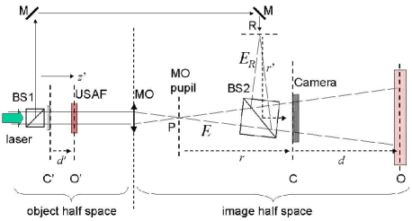
Figure 1: Typical holographic microscopy setup. USAF: USAF target located in plane O’; MO: microscope objective that images the USAF target in plane O; BS1, BS2: beam splitters; M: mirror. $E$ and $E_{R}$: signal and reference fields; Note that BS2 is angularly tilted in order to perform off axis holography.

To illustrate reconstruction, let us consider a typical holographic microscopy setup (see Fig. 1). The object is located in plane O’ and is imaged by the microscope objective MO in plane O. The camera located in plane C records the hologram $H$ that is the interference pattern of the signal field $E$ with the reference field $E_{R}$. The purpose is to reconstruct the amplitude and the phase of the field scattered by the object in the object plane O’, and near this plane (if the object is thick or if one want to measure the wave field). Before making reconstruction, one need to calibrate the setup to get the reconstruction parameters, which depends on the optical elements in the image half space: location of MO, BS2 and camera, BS2 angular tilt and direction and curvature of the reference beam (i.e. location of point R). Once the calibration of the setup is made, the reconstruction must be valid for any object. This means that one can modify all the optical elements in the object half space (object and object location, direction and curvature of the illumination beam), but the optical elements in the image half space must remains unchanged.

The reconstruction methods mentioned above montfort2006npl ; ferraro2003ciw ; montfort2006npl ; colomb2006npl ; colomb2006tac ; colomb2006apa made reconstruction in the image half space. This means that the image of the object in plane O is reconstructed by propagating the hologram over a distance $d$ from C to O. This propagation is calculated in free space, by using either the one Fourier Transform (1-FFT) method schnars1994direct , or the angular spectrum (2-FFT) method yun2004dms . However, reconstruction in the image half space becomes difficult when varying the location of the object along $z^{\prime}$, or when imaging thick objects. Indeed, the location of the image O and the reconstruction distance $d=|\textrm{CO}|$ strongly depend on the object location $z^{\prime}$, which complexifies the reconstruction process. If the object is located near plane C’, which is imaged by MO on the camera (i.e. on plane C), we get $d\simeq$ 0. The 2-FFT reconstruction method, which is well suited to small $d$, should thus be preferred. Conversely, if the object is close to the MO focal plane, we get $d\rightarrow\infty$, and the 1-FFT method should be used. This point tends to be problematic if we consider reconstruction of both amplitude and phase of of the light scattered by a thick 3D sample, or if one want to measure the wave field. As a matter of fact, it prevents experimental setup calibration to remain valid for the entire sample thickness. Making the setup calibration independent of the sample position according to MO is therefore an issue to tackle.

Here, we propose to consider that the recorded signal $|E+E_{R}|^{2}$ represents the hologram $H^{\prime}$ of the field scattered by the object in the plane of the image of the camera (i.e. in plane C’). The reconstruction is therefore made in the object half space, by propagating hologram $H^{\prime}$ over a distance $d^{\prime}=|\textrm{C'O'}|$ from plane C’ to plane O’. Since $d^{\prime}$ is always small (a few microns), the 2-FFT methodyun2004dms is well adapted in all cases ($d\simeq 0$ or $d\simeq\infty$), which notably simplifies reconstruction algorithms. Moreover, if the calibration is done well, this reconstruction can be made with orthogonal $x^{\prime}$, $y^{\prime}$ and $z^{\prime}$ axes, while keeping constant the pixel pitches in the $x^{\prime}$ and $y^{\prime}$ axes.

II Calculation of the hologram of the field in plane C’

The hologram $H$ recorded by the camera in plane C is:

$$H = |E+E_{R}|^{2}$$

$$= |E|^{2}+|E_{R}|^{2}+EE^{*}_{R}+E^{*}E_{R}$$

where $E$ and $E_{R}$ are the signal and reference fields in plane C. Because of the microscope objective MO, the curvature of the reference field and the off axis angular tilt, the phase of $H$ in plane C is not equal to the phase of the signal field in camera conjugate plane C’, from which the object half space reconstruction will be made. Moreover, the +1 grating order term $EE^{*}_{R}$ that is proportional to the field $E$ must be selectively filtered. To perform the reconstruction from the field $E$ in plane C’, it is thus necessary to manipulate the data to compensate for these phase effects and to select the $EE^{*}_{R}$ term that is proportional to $E$ montfort2006purely . This manipulation of the data must be made with few calibration parameters that characterize the optical elements of the image half space part of the setup, and that do not depends on the the object i.e. on the optical elements of the object half space.

II.1 The phase curvature in the camera plane C

Let us analyze first the phase curvature of $EE^{*}_{R}$ in plane C. For that purpose, we will consider a “gedanken experiment” without object in which the illumination beam is plane wave beam oriented along the optical axis $z^{\prime}$. The field $E$ is thus flat in plane C’.

This plane wave is focused by MO at point P in the MO pupil plane. The signal complex field $E$ exhibit thus a phase factor equal to $e^{jk(x^{2}+y^{2})/2r}$, where $k=2\pi/\lambda$ is the modulus of the wavevector in air, and where $r$ is the radius of curvature of the wavefront that is equal to the MO pupil to camera distance $r=|\textrm{PC}|$. Similarly, the phase of the complex conjugate of the reference field $E_{R}^{*}$ is $e^{-jk(x^{2}+y^{2})/2r^{\prime}}$ where $r^{\prime}=|\textrm{RC}|$ is the radius of curvature of $E_{R}$ (with $r^{\prime}=\infty$ if the reference beam is a plane wave). This means that the phase of the +1 grating order term $EE^{*}_{R}$ in plane C is $e^{+jk(x^{2}+y^{2})/2r^{\prime\prime}}$ with $1/r^{\prime\prime}=1/r-1/r^{\prime}$.

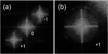
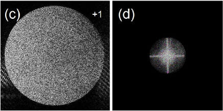
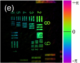
Figure 2: (a) Reconstructed USAF target hologram in the pupil plane ${\tilde{H}_{1}}(k_{x},k_{y})$ ($1024\times 1024$ pixels). (b) Zoom of the +1 grating order of ($512\times 512$ pixels). (c) Pupil image obtained with ground glass imaged with an $\times 10$ MO. (d) Fourier space filtered hologram ${\tilde{H}_{2}}(k_{x},k_{y})$ of the +1 grating order made with a circular crop of the MO pupil image (radius $r_{k}$=162 pixels) followed by a translation of the selected zone in the center of the Fourier space. (e) Spatially filtered hologram $H^{\prime}_{2}(x,y)$ with proper phase correction. Arbitrary scale brightness is $|H_{...}|^{2}$, color is phase i.e. $\arg H_{...}$.

II.2 Phase curvature correction by reconstruction of the MO pupil

Let us reconstruct the image ${\tilde{H}}_{1}(k_{x},k_{y})$ of the MO pupil by using the 1-FFT method or Fourier reconstruction methodschnars1994direct . We have thus:

$${\tilde{H}_{1}}(k_{x},k_{y})=\textrm{FFT}\left[e^{-jk(x^{2}+y^{2})/2r^{\prime\prime}}~{}H(x,y)\right]$$ (2)

where $e^{-jk(x^{2}+y^{2})/2r^{\prime\prime}}$ is equal to $e^{-jk(x^{2}+y^{2})/2r}$ $\times$ $e^{+jk(x^{2}+y^{2})/2r^{\prime}}$. The first phase factor $e^{-jk(x^{2}+y^{2})/2r}$ is the 1-FFT propagation kernel over a distance $r$, while the second factor $e^{+jk(x^{2}+y^{2})/2r^{\prime}}$ compensates the curvature of $E_{R}^{*}$. Since the back focal point P is located within the MO pupil plane, the propagation distance $r$ is equal to $|\textrm{PC}|$. This means that the reconstruction phase factor $e^{-jk(x^{2}+y^{2})/2r^{\prime\prime}}$ exactly compensates the phase curvature $e^{+jk(x^{2}+y^{2})/2r^{\prime\prime}}$ of $EE_{R}^{*}$ calculated in section II.1 .

To determine $r^{\prime\prime}$, we propose to reconstruct the MO pupil images $|{\tilde{H}_{1}}|^{2}$ by adjusting $r^{\prime\prime}$ so as to obtain the sharpest image of the pupil edge. Since the we have validated our reconstruction with a USAF target located in near plane C’, we have reconstruct the pupil image $|{\tilde{H}_{1}}(k_{x},k_{y})|^{2}$ obtained with the target in plane C’, and displayed it on Fig.2 (a). 3 bright zones corresponding the +1, -1 and zero grating orders are visible. These zones are separated because of the off axis tilt angle. Here, the reconstruction parameter $r^{\prime\prime}$ has been properly adjusted, and the pupil edge of the +1 grating order zone is sharp as seen on the zoom displayed on Fig.2 (b).

Nevertheless, the pupil edge is dark on Fig.2 (a) and (b), because the USAF target scatters light over quite narrow angles. The adjustment of $r^{\prime\prime}$ is thus quite difficult. It is easier to adjust $r^{\prime\prime}$ with an object that scatters more light, like a ground glass located in front of MO. Figure 2 (c) shows an example of a pupil reconstruction made with such a ground glass. Let us notice here that the adjustment of $r^{\prime\prime}$ can be made with the object of interest itself without any previous calibration of the setup. This has been done in absil2010photothermal .

II.3 Spatial filtering and off axis phase correction

To perform the spatial filtering that selects $EE_{R}^{*}$ and to compensate the off axis angular tilt, we propose to crop the data within the circular MO pupil image (which is sharp), and to translate the cropped zone to the center of the calculation grid. The spatial filtering is made by the crop, while the off axis compensation is made by the translation.

The filtered and phase-corrected hologram of the pupil in the Fourier space ${\tilde{H}}_{2}$ is thus:

$${\tilde{H}}_{2}(\textbf{k}_{xy}) = {\tilde{H}_{1}}(\textbf{k}_{xy}+d\textbf{k}_{xy})~{}~{}~{}~{}~{}~{}~{}~{}\textrm{if }~{}~{}|\textbf{k}_{xy}|<r_{k}$$ (3)

$$= 0~{}~{}~{}~{}~{}~{}~{}~{}~{}~{}~{}~{}~{}~{}~{}~{}~{}~{}~{}~{}~{}~{}~{}~{}~{}~{}~{}\textrm{if not}$$

where $\textbf{k}_{xy}=(k_{x},k_{y})$, $d\textbf{k}_{xy}$ is the translation that moves the +1 pupil image in the center of the Fourier space, and $r_{k}$ the pupil radius. The corresponding real space hologram ${H}_{2}$ is:

$$H_{2}(x,y) = \textrm{FFT}^{-1}\left[{\tilde{H}}_{2}(k_{x},k_{y})~{}\right]$$ (4)

where $\textrm{FFT}^{-1}$ is the reverse 2D Fourier transform.

We have displayed $|H_{2}(x,y)|^{2}$ on Fig. 2(e) with phase displayed with color. Since the USAF target is located in plane C’, the image of the target is sharp. Moreover the phase, which is displayed in color, is the same in all point of the image, like the phase of the field $E$ in plane C’. This means that the phase has been properly corrected.

II.4 Object/image half space holograms

In the previous calculation, the holograms $H$, $\tilde{H}_{1}$, $\tilde{H}_{2}$ … are matrices of data, that represent the field either in the image or the object half space.

To avoid any confusion, we will consider that $H$, $\tilde{H}_{1}$, $\tilde{H}_{2}$ … are the holograms, and $x,y,k_{x},k_{y}$ the coordinates in the image half space. The pitch is $\Delta x$ for $x$ and $y$, and $\Delta k=2\pi/(N\Delta x)$ for $k_{x}$ and $k_{y}$ (where $\Delta x$ is the camera pixel size, and $N$ the size of the calculation grid) .

On the other hand, $H^{\prime}$, $\tilde{H}^{\prime}_{1}$, $\tilde{H}^{\prime}_{2}$ … are the holograms, and $x^{\prime},y^{\prime},k^{\prime}_{x}$ and $k^{\prime}_{y}$ the coordinates in the object half space. The pitch is $\Delta^{\prime}x=\Delta^{\prime}x/G$ for $x^{\prime}$ and $y^{\prime}$, and $\Delta^{\prime}k=G\Delta^{\prime}k$ for $k^{\prime}_{x}$ and $k^{\prime}_{y}$ (where $G\gg 1$ is the MO transverse gain from plane C’ to plane C). We have thus:

$$H^{\prime}_{...}(x^{\prime},y^{\prime}) = H_{...}(x,y)$$ (5)

$$\tilde{H}^{\prime}_{...}(k^{\prime}_{x},k^{\prime}_{y}) = \tilde{H}_{...}(k_{x},k_{y})$$

with $x^{\prime}=x/G$, $y^{\prime}=y/G$ , $k^{\prime}_{x}=k_{x}G$ and $k^{\prime}_{y}=k_{y}G$.

III Reconstruction of the field in any plane

III.1 Reconstruction in the object half space

We have calculated the phase-corrected hologram $H^{\prime}_{2}$ in plane C’ in section II by Eq.4 and Eq.5. The image $H^{\prime}_{3}(x^{\prime},y^{\prime},z^{\prime})$ of the object in any $z^{\prime}$ plane is reconstructed by using the 2-FFT reconstruction method (also known as the convolution method) yun2004dms from $H^{\prime}_{2}(x^{\prime},y^{\prime})$. Since ${\tilde{H}}^{\prime}_{2}=\textrm{FFT}(H^{\prime}_{2})$, we have:

$$H^{\prime}_{3}(x^{\prime},y^{\prime},z^{\prime})=\\ \textrm{FFT}^{-1}\left[e^{j(k_{x}^{\prime 2}+k_{y}^{\prime 2})z^{\prime}/2k_{m}}{\tilde{H}}^{\prime}_{2}(k^{\prime}_{x},k^{\prime}_{y})\right]$$ (6)

where $e^{j(k_{x}^{\prime 2}+k_{y}^{\prime 2})z^{\prime}/2k_{m}}$ is the 2-FFT propagation kernel over distance $z^{\prime}$. The origin $z^{\prime}=0$ corresponds thus to plane C’. Note that since propagation from C’ to O’ takes place in a medium (air, water or oil) of refractive index $n_{\rm m}$, $k$ has been replaced by $k_{\rm m}=n_{\rm m}k$ in the propagation kernel.

III.2 Reconstruction in the image half space

Equation (5) makes the correspondance of the holograms $H_{...}$ and $H^{\prime}_{...}$ in planes C and C’. It can be generalized for any plane by:

$$H^{\prime}_{...}(x^{\prime},y^{\prime},z^{\prime}) = H_{...}(x,y,z)$$ (7)

$$\tilde{H}^{\prime}_{...}(k^{\prime}_{x},k^{\prime}_{y},z^{\prime}) = \tilde{H}_{...}(k_{x},k_{y},z)$$

where $z$ is a formal coordinate that is not equal to $d=|\textrm{CO}|$. We can now calculate $H_{3}(x,y,z)$ by using a relation formally equivalent to Eq. (6). We get:

$$H_{3}(x,y,z)=\textrm{FFT}^{-1}\left(e^{j(k_{x}^{2}+k_{y}^{2})z/2k}{\tilde{H}}_{2}(k_{x},k_{y})\right)$$

Since propagation in image half space is made in air, we have chosen in Eq. (III.2) a propagation kernel that involves $k$ (instead of $k_{\rm m}$). Equations (6) and (III.2) yield exactly the same calculations on the discrete data of the calculation grid if we have

$$z = z^{\prime}G^{2}/n_{m}$$ (9)

This equation defines the formal coordinate $z$.

III.3 The afocal device that makes the reconstructions in the object and image half space equivalent

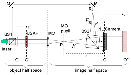
Figure 3: Reinterpretation of the holographic microscopy setup. USAF: USAF target located in plane O’; MO: microscope objective; NL: numerical lens of focal $r$ located in the camera plane C; MO + NL: afocal optical device that images the USAF target in plane O”.

The reconstruction made in the image half space by Eq. III.2 and Eq. 9 can be reinterpreted quite simply. The phase curvature of the reference beam (phase factor $e^{jk(x^{2}+y^{2})/2r^{\prime}}$) combined with the numerical phase factor $e^{jk(x^{2}+y^{2})/2r^{\prime\prime}}$ used to image the MO pupil (and to correct the phase in plane C’) is equivalent to a Numerical Lens (NL) of focal length $r$ (phase factor $e^{jk(x^{2}+y^{2})/2r}$) located in the camera plane C (see Fig. 3). Since the MO and NL have a common focal point P, MO and NL form an afocal optical device, with an overall transverse gain $G$ and a longitudinal gain ${G^{2}}/{n_{m}}$. Performing the reconstruction either in the object or image half space is thus totally equivalent.

The reconstruction made in the image half space with the afocal optical device is close to the reconstruction called ”Image Plane Approach” by Monfort et al. montfort2006purely . Nevertheless, these authors consider a varying magnification factor, which involves explicitly the size of the image of the object in plane O, and which depends strongly on the location of the object. But the varying Monfort et al. magnification and the varying object magnification (plane O’ to image plane O: see Fig.1) compensate yielding a constant magnification (object in plane O’ to reconstructed image in plane O”: see Fig.3), which is simply equal to G.

IV Experimental validation

To validate our reconstruction method, we have made a test experiment with a $\lambda=$785 nm laser (Sanyo DL-7140-201) by imaging an USAF target with an oil immersion ($n_{m}=1.518$) Microscope Objective MO (NA=1.4 $\times$60) and a holographic setup built by modifying a commercial upright microscope. A detailed description of the setup is given in reference verrier2014laser . The holograms are recorded for $m=0...59$ different positions $z^{\prime}_{m}$ of the target along $z^{\prime}$, the positions being adjusted manually with steps of $\Delta z^{\prime}=2.5~{}\mu$m. The sharpest image (nearly focused without any correction) corresponds to location $m=29$. The holograms are recorded with a PCO Pixelfly camera ($1280\times 1024$ square pixels of size $\Delta x=6.7~{}\mu$m), and the measured data are cropped into a $1024\times 1024$ calculation grid.

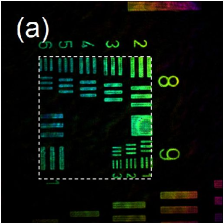
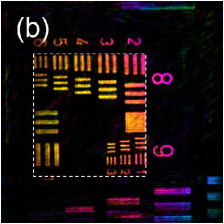
Figure 4: (a) Reconstructed hologram $H^{\prime}_{3}$ of the USAF target for positions $m=29$ made with $z^{\prime}=0$ (a), and $m=0$ with $z^{\prime}\simeq-72.5\mu$m (b). Arbitrary scale brightness is intensity i.e. $|H^{\prime}_{3}|^{2}$, color is phase i.e. $\arg H^{\prime}_{3}$. The white dashed line rectangles ($517\times 567$ pixels) seen are visual guides, whose sizes are exactly the same size, and positions slightly shifted.

The hologram $H^{\prime}_{3}$ of the USAF target at position $m=29$ is displayed on Fig. 4 (a). Since the USAF target is nearly focused without any correction, reconstruction is made with $z^{\prime}=0$. Moreover, since the phase correction has been made, the phase of the illumination beam is flat i.e. the color is approximately the same within the whole USAF target. We have then used the $m=29$ USAF image, which is sharp, to calibrate $G$. We got $G=74.61$.

We have then reconstructed the USAF target for every position, from $m=0$ to $m=59$. Figure 4 (b) shows for example the USAF image for position $m=0$. As expected, the size and location of the USAF image remains the same, showing that the $x$ and $y$ scales are conserved. This can be verified by comparing Fig. 4 (a) and (b). For positions $m=0$ (corresponding to $z^{\prime}\simeq-72.5~{}\mu$m) and $m=29$ ($z^{\prime}\simeq 0$), the size of the USAF target is exactly preserved (see white dashed rectangle) while the position is slightly shifted.

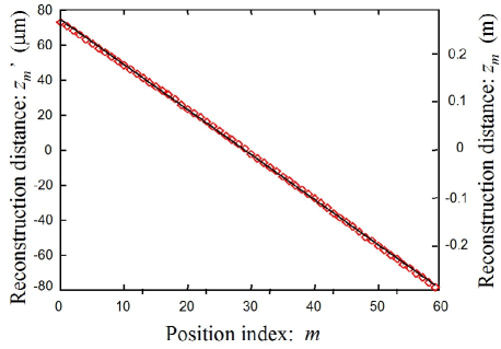
Figure 5: Reconstruction distances $z^{\prime}_{m}$ and $z_{m}$ as function of the USAF target location $m$ (red points) and best linear fit (black solid line).

For each position $m$, we have reconstructed the hologram $H^{\prime}_{3}(x^{\prime},y^{\prime},z^{\prime}_{m})$ by adjusting $z^{\prime}_{m}$ (or $z_{m}$) so as to obtain the sharpest image. As the USAF target is an “amplitude object”, we have adjust $z^{\prime}_{m}$ by using the ”focus plane detection criteria” of Dubois et al. dubois2006focus . Since the position and size of the image remain the same, this automatic adjustment of $z^{\prime}_{m}$ works well. Figure 5 shows the reconstruction distances $z^{\prime}_{m}$ obtained by this method. As can be seen, $z^{\prime}_{m}$ varies linearly with $m$ with a slope $dz^{\prime}_{m}/dm=-2.56~{}\mu$m which corresponds to the mechanical displacement, and with an offset $m=28.97$ that is nearly equal to the location $m=29$, where the USAF target is on focus on the camera.

V Remark on the calibration of the setup

In section II.1, we have calibrated the setup i.e. determine $r^{\prime\prime}$ and $d\textbf{k}_{xy}$ by reconstructing the image of the pupil with an object that scatters enough light. $r^{\prime\prime}$ is adjusted to get the sharpest pupil edges, and $d\textbf{k}_{xy}$ by translating the pupil in the center of the Fourier space.

In section IV, we have seen that the the size and location (in $x$ and $y$ directions) of the reconstructed image of the USAF target do not change by moving the target along $z^{\prime}$. This property provides a second calibration method. One can move an object along the $z^{\prime}$ direction and consider 2 different positions the object, for example $z^{\prime}=-72.5\mu$m, and $z^{\prime}=0$. One can then record the holograms and reconstruct the images of the object for these 2 positions, as done in Fig.4 (a) and (b). One can then adjust $r^{\prime\prime}$ in order to get the same size for the 2 reconstructed images, and adjust and $d\textbf{k}_{xy}$ to get the same positions. In the example of Fig.4, the adjustment of $r^{\prime\prime}$ is nearly perfect (since the USAF sizes are exactly the same on (a) and (b) ), while the adjustment of $d\textbf{k}_{xy}$ could be improved (since the positions are slightly shifted). Our experience is that second calibration method (size and position of 2 reconstructed images with different $z^{\prime}$) yields more precise calibration than the first method (pupil sharpness and pupil translation).

The two proposed calibration methods do not require a flat phase illumination like the methods based on the phase flatness of the reconstructed image colomb2006apa . Note also that the reconstruction direction $z^{\prime}$ depends on the calibration method which is used to get $d\textbf{k}_{xy}$. If the phase flatness is used, the $z^{\prime}$ axis is the direction of the illumination beam. If the translation of pupil image is used (first calibration method), $z^{\prime}$ is parallel to the line that joins the pupil center to the camera center. If the position of reconstructed image of the object (USAF target) is used (second calibration method), $z^{\prime}$ is parallel with the $z$ motion. This last method is the best method when a modified commercial microscope is used to make holography, since the $z^{\prime}$ axis coincides with the microscope $z$ axis.

VI Remark on construction with tube lens

All the results presented here remains valid when a tube lens placed between the pupil P and the beam splitter BS2. In the ”gedanken experiment” with a plane wave illumination beam, the tube lens changes the curvature of the field $E$ in plane C , i.e. $r$. The calibration parameter $r^{\prime\prime}$, and the NL focal lens $r$ are thus both changed. By using the second calibration method, $r^{\prime\prime}$ is adjusted so that the size of the reconstructed image object is not dependent on the object position $z^{\prime}$. This means that the ensemble of lenses MO+tube lens+ NL still constitute an afocal device, with transverse and longitudinal magnifications $G$ and $G^{2}/n_{m}$.

VII Conclusion

We have proposed a holographic microscopy reconstruction method which propagates the hologram in the object half space, in the vicinity of the object. Since the reconstruction phase, the reference phase curvature and MO form an afocal device, the reconstruction can be interpreted as occurring equivalently in the object or in image half space.

The reconstruction method has been validated with a USAF target which has been imaged with a high numerical aperture microscope objective MO for different locations of the target along the longitudinal axis $z^{\prime}$. We have verified that the reconstruction is made with orthogonal axes $x^{\prime}$, $y^{\prime}$ and $z^{\prime}$, and that the pixel pitches $x^{\prime}$, $y^{\prime}$ and $z^{\prime}$ do not depend on the USAF target location. The experimental test has been made with a plane illumination beam oriented along the $z$ axis, and we have verify that the reconstructed phase (colors on Fig. 4 (a) and (b) ) varies slowly with $x,y$. The proposed reconstruction is compatible with spherical or dark field illumination  atlan2008heterodyne ; absil2010photothermal ; warnasooriya2010imaging ; verpillat2011dark .

Two calibration methods, which do not require plane wave illumination have been proposed. The first method is based on the reconstruction of the MO pupil, with an object that scatters light. This method can be used with holograms of interest which have recorded without proper calibration of the setup, and has been used in that case absil2010photothermal . The second method, which is more precise, requires to translate an object along the $z^{\prime}$ axis and to record two holograms for two different $z^{\prime}$.

References

- (1) U. Schnars and W. Jüptner, “Direct recording of holograms by a CCD target and numerical reconstruction,” Appl. Opt. 33, 179–181 (1994).
- (2) P. Picart and J. Leval, “General theoretical formulation of image formation in digital Fresnel holography,” J. Opt. Soc. Am. A 25, 1744–1761 (2008).
- (3) H. Yun, S. Jeong, J. Kang, and C. Hong, “3-Dimensional Micro-structure Inspection by Phase-Shifting Digital Holography,” Key Eng. Mater. 270, 756–761 (2004).
- (4) F. Zhang, I. Yamaguchi, and L. Yaroslavsky, “Algorithm for reconstruction of digital holograms with adjustable magnification,” Opt. Lett. 29, 1668–1670 (2004).
- (5) E. Cuche, F. Belivacqua, and C. Depeursinge, “Digital holography for quantitative phase-contrast imaging,” Opt. Lett. 24, 291–293 (1999).
- (6) P. Ferraro, G. Coppola, S. De Nicola, A. Finizio, and G. Pierattini, “Digital holographic microscope with automatic focus tracking by detecting sample displacement in real time,” Opt. Lett. 28, 1257–1259 (2003).
- (7) F. Charrière, A. Marian, F. Montfort, J. Kuehn, T. Colomb, E. Cuche, P. Marquet, and C. Depeursinge, “Cell refractive index tomography by digital holographic microscopy,” Opt. Lett. 31, 178–180 (2006).
- (8) J. Garcia-Sucerquia, W. Xu, S. Jericho, P. Klages, M. Jericho, and H. Kreuzer, “Digital in-line holographic microscopy,” Appl. Opt. 45, 836–850 (2006).
- (9) S. Lee, Y. Roichman, G. Yi, S. Kim, S. Yang, A. van Blaaderen, P. van Oostrum, and D. Grier, “Characterizing and tracking single colloidal particles with video holographic microscopy,” Opt. Express 15, 18275–18282 (2007).
- (10) J. Sheng, E. Malkiel, and J. Katz, “Digital holographic microscope for measuring three-dimensional particle distributions and motions,” Appl. Opt. 45, 3893–3901 (2006).
- (11) F. Montfort, F. Charrière, T. Colomb, E. Cuche, P. Marquet, and C. Depeursinge, “Purely numerical compensation for microscope objective phase curvature in digital holographic microscopy: influence of digital phase mask position,” J. Opt. Soc. Am. A 23, 2944–2953 (2006).
- (12) P. Ferraro, S. De Nicola, A. Finizio, G. Coppola, S. Grilli, C. Magro, and G. Pierattini, “Compensation of the inherent wave front curvature in digital holographic coherent microscopy for quantitative phase-contrast imaging,” Appl. Opt. 42, 1938–1946 (2003).
- (13) T. Colomb, F. Montfort, J. Kühn, N. Aspert, E. Cuche, A. Marian, F. Charrière, S. Bourquin, P. Marquet, and C. Depeursinge, “Numerical parametric lens for shifting, magnification, and complete aberration compensation in digital holographic microscopy,” J. Opt. Soc. Am. A 23, 3177–3190 (2006).
- (14) T. Colomb, J. Kühn, F. Charrière, C. Depeursinge, P. Marquet, and N. Aspert, “Total aberrations compensation in digital holographic microscopy with a reference conjugated hologram,” Opt. Express 14, 4300–4306 (2006).
- (15) T. Colomb, E. Cuche, F. Charrière, J. Kühn, N. Aspert, F. Montfort, P. Marquet, and C. Depeursinge, “Automatic procedure for aberration compensation in digital holographic microscopy and applications to specimen shape compensation,” Appl. Opt. 45, 851–863 (2006).
- (16) T. Zhang and I. Yamaguchi, “Three-dimensional microscopy with phase-shifting digital holography,” Opt. Lett. 23, 1221–1223 (1998).
- (17) E. Cuche, P. Marquet, and C. Depeursinge, “Simultaneous amplitude-contrast and quantitative phase-contrast microscopy by numerical reconstruction of Fresnel off-axis holograms,” Appl. Opt. 38, 6994–7001 (1999).
- (18) F. Montfort, F. Charrière, T. Colomb, E. Cuche, P. Marquet, and C. Depeursinge, “Purely numerical compensation for microscope objective phase curvature in digital holographic microscopy: influence of digital phase mask position,” J. Opt. Soc. Am. A 23, 2944–2953 (2006).
- (19) E. Cuche, P. Marquet, and C. Depeursinge, “Spatial filtering for zero-order and twin-image elimination in digital off-axis holography,” Appl. Opt. 39, 4070–4075 (2000).
- (20) N. Verrier, D. Alexandre, and M. Gross, “Laser doppler holographic microscopy in transmission: application to fish embryo imaging,” Opt. Express 22, 9368–9379 (2014).
- (21) F. Dubois, C. Schockaert, N. Callens, and C. Yourassowsky, “Focus plane detection criteria in digital holography microscopy by amplitude analysis,” Opt. Express 14, 5895–5908 (2006).
- (22) M. Atlan, M. Gross, P. Desbiolles, É. Absil, G. Tessier, and M. Coppey-Moisan, “Heterodyne holographic microscopy of gold particles,” Opt. Lett. 33, 500–502 (2008).
- (23) E. Absil, G. Tessier, M. Gross, M. Atlan, N. Warnasooriya, S. Suck, M. Coppey-Moisan, D. Fournier, “Photothermal heterodyne holography of gold nanoparticles,” Opt. Express 18, 780–786 (2010).
- (24) N. Warnasooriya, F. Joud, P. Bun, G. Tessier, M. Coppey-Moisan, P. Desbiolles, M. Atlan, M. Abboud, M. Gross, “Imaging gold nanoparticles in living cell environments using heterodyne digital holographic microscopy,” Opt. Express 18, 3264–3273 (2010).
- (25) F. Verpillat, F. Joud, P. Desbiolles, M. Gross, “Dark-field digital holographic microscopy for 3d-tracking of gold nanoparticles,” Opt. Express 19, 26044–26055 (2011).