Inferring Graphs from Cascades: A Sparse Recovery Framework

Abstract

In the Network Inference problem, one seeks to recover the edges of an unknown graph from the observations of cascades propagating over this graph. In this paper, we approach this problem from the sparse recovery perspective. We introduce a general model of cascades, including the voter model and the independent cascade model, for which we provide the first algorithm which recovers the graph’s edges with high probability and ${\cal O}(s\log m)$ measurements where $s$ is the maximum degree of the graph and $m$ is the number of nodes. Furthermore, we show that our algorithm also recovers the edge weights (the parameters of the diffusion process) and is robust in the context of approximate sparsity. Finally we prove an almost matching lower bound of $\Omega(s\log\frac{m}{s})$ and validate our approach empirically on synthetic graphs.

1 Introduction

Graphs have been extensively studied for their propagative abilities: connectivity, routing, gossip algorithms, etc. A diffusion process taking place over a graph provides valuable information about the presence and weights of its edges. Influence cascades are a specific type of diffusion processes in which a particular infectious behavior spreads over the nodes of the graph. By only observing the “infection times” of the nodes in the graph, one might hope to recover the underlying graph and the parameters of the cascade model. This problem is known in the literature as the Network Inference problem.

More precisely, solving the Network Inference problem involves designing an algorithm taking as input a set of observed cascades (realisations of the diffusion process) and recovers with high probability a large fraction of the graph’s edges. The goal is then to understand the relationship between the number of observations, the probability of success, and the accuracy of the reconstruction.

The Network Inference problem can be decomposed and analyzed “node-by-node”. Thus, we will focus on a single node of degree $s$ and discuss how to identify its parents among the $m$ nodes of the graph. Prior work has shown that the required number of observed cascades is $\mathcal{O}(poly(s)\log m)$ (Netrapalli & Sanghavi, 2012; Abrahao et al., 2013).

A more recent line of research (Daneshmand et al., 2014) has focused on applying advances in sparse recovery to the network inference problem. Indeed, the graph can be interpreted as a “sparse signal” measured through influence cascades and then recovered. The challenge is that influence cascade models typically lead to non-linear inverse problems and the measurements (the state of the nodes at different time steps) are usually correlated. The sparse recovery literature suggests that $\Omega(s\log\frac{m}{s})$ cascade observations should be sufficient to recover the graph (Donoho, 2006; Candes & Tao, 2006). However, the best known upper bound to this day is $\mathcal{O}(s^{2}\log m)$ (Netrapalli & Sanghavi, 2012; Daneshmand et al., 2014)

The contributions of this paper are the following:

• we formulate the Graph Inference problem in the context of discrete-time influence cascades as a sparse recovery problem for a specific type of Generalized Linear Model. This formulation notably encompasses the well-studied Independent Cascade Model and Voter Model.

• we give an algorithm which recovers the graph’s edges using $\mathcal{O}(s\log m)$ cascades. Furthermore, we show that our algorithm is also able to efficiently recover the edge weights (the parameters of the influence model) up to an additive error term,

• we show that our algorithm is robust in cases where the signal to recover is approximately $s$-sparse by proving guarantees in the stable recovery setting.

• we provide an almost tight lower bound of $\Omega(s\log\frac{m}{s})$ observations required for sparse recovery.

The organization of the paper is as follows: we conclude the introduction by a survey of the related work. In Section 2 we present our model of Generalized Linear Cascades and the associated sparse recovery formulation. Its theoretical guarantees are presented for various recovery settings in Section 3. The lower bound is presented in Section 4. Finally, we conclude with experiments in Section 5.

Related Work

The study of edge prediction in graphs has been an active field of research for over a decade (Liben-Nowell & Kleinberg, 2008; Leskovec et al., 2007; Adar & Adamic, 2005). (Gomez Rodriguez et al., 2010) introduced the Netinf algorithm, which approximates the likelihood of cascades represented as a continuous process. The algorithm was improved in later work (Gomez-Rodriguez et al., 2011), but is not known to have any theoretical guarantees beside empirical validation on synthetic networks. Netrapalli & Sanghavi (2012) studied the discrete-time version of the independent cascade model and obtained the first ${\cal O}(s^{2}\log m)$ recovery guarantee on general networks. The algorithm is based on a likelihood function similar to the one we propose, without the $\ell_{1}$-norm penalty. Their analysis depends on a correlation decay assumption, which limits the number of new infections at every step. In this setting, they show a lower bound of the number of cascades needed for support recovery with constant probability of the order $\Omega(s\log(m/s))$. They also suggest a Greedy algorithm, which achieves a ${\cal O}(s\log m)$ guarantee in the case of tree graphs. The work of (Abrahao et al., 2013) studies the same continuous-model framework as (Gomez Rodriguez et al., 2010) and obtains an ${\cal O}(s^{9}\log^{2}s\log m)$ support recovery algorithm, without the correlation decay assumption. (Du et al., 2013) propose a similar algorithm to ours for recovering the weights of the graph under a continuous-time independent cascade model, without proving theoretical guarantees.

Closest to this work is a recent paper by Daneshmand et al. (2014), wherein the authors consider a $\ell_{1}$-regularized objective function. They adapt standard results from sparse recovery to obtain a recovery bound of ${\cal O}(s^{3}\log m)$ under an irrepresentability condition (Zhao & Yu, 2006). Under stronger assumptions, they match the (Netrapalli & Sanghavi, 2012) bound of ${\cal O}(s^{2}\log m)$, by exploiting similar properties of the convex program’s KKT conditions. In contrast, our work studies discrete-time diffusion processes including the Independent Cascade model under weaker assumptions. Furthermore, we analyze both the recovery of the graph’s edges and the estimation of the model’s parameters, and achieve close to optimal bounds.

The work of (Du et al., 2014) is slightly orthogonal to ours since they suggest learning the influence function, rather than the parameters of the network directly.

2 Model

We consider a graph ${\cal G}=(V,E,\Theta)$, where $\Theta$ is a $|V|\times|V|$ matrix of parameters describing the edge weights of $\mathcal{G}$. Intuitively, $\Theta_{i,j}$ captures the “influence” of node $i$ on node $j$. Let $m\equiv|V|$. For each node $j$, let $\theta_{j}$ be the $j^{th}$ column vector of $\Theta$. A discrete-time Cascade model is a Markov process over a finite state space ${\{0,1,\dots,K-1\}}^{V}$ with the following properties:

1. Conditioned on the previous time step, the transition events between two states in $\{0,1,\dots,K-1\}$ for each $i\in V$ are mutually independent across $i\in V$.

2. Of the $K$ possible states, there exists a contagious state such that all transition probabilities of the Markov process can be expressed as a function of the graph parameters $\Theta$ and the set of “contagious nodes” at the previous time step.

3. The initial probability over ${\{0,1,\dots,K-1\}}^{V}$ is such that all nodes can eventually reach a contagious state with non-zero probability. The “contagious” nodes at $t=0$ are called source nodes.

In other words, a cascade model describes a diffusion process where a set of contagious nodes “influence” other nodes in the graph to become contagious. An influence cascade is a realisation of this random process, i.e. the successive states of the nodes in graph ${\cal G}$. Note that both the “single source” assumption made in (Daneshmand et al., 2014) and (Abrahao et al., 2013) as well as the “uniformly chosen source set” assumption made in (Netrapalli & Sanghavi, 2012) verify condition 3. Also note that the multiple-source node assumption does not reduce to the single-source assumption, even under the assumption that cascades do not overlap. Imagining for example two cascades starting from two different nodes; since we do not observe which node propagated the contagion to which node, we cannot attribute an infected node to either cascade and treat the problem as two independent cascades.

In the context of Network Inference, (Netrapalli & Sanghavi, 2012) focus on the well-known discrete-time independent cascade model recalled below, which (Abrahao et al., 2013) and (Daneshmand et al., 2014) generalize to continuous time. We extend the independent cascade model in a different direction by considering a more general class of transition probabilities while staying in the discrete-time setting. We observe that despite their obvious differences, both the independent cascade and the voter models make the network inference problem similar to the standard generalized linear model inference problem. In fact, we define a class of diffusion processes for which this is true: the Generalized Linear Cascade Models. The linear threshold model is a special case and is discussed in Section 6.

2.1 Generalized Linear Cascade Models

Let susceptible denote any state which can become contagious at the next time step with a non-zero probability. We draw inspiration from generalized linear models to introduce Generalized Linear Cascades:

Definition 1.

Let $X^{t}$ be the indicator variable of “contagious nodes” at time step $t$. A generalized linear cascade model is a cascade model such that for each susceptible node $j$ in state $s$ at time step $t$, the probability of $j$ becoming “contagious” at time step $t+1$ conditioned on $X^{t}$ is a Bernoulli variable of parameter $f(\theta_{j}\cdot X^{t})$:

$$\mathbb{P}(X^{t+1}_{j}=1|X^{t})=f(\theta_{j}\cdot X^{t})$$ (1)

where $f:\mathbb{R}\rightarrow[0,1]$

In other words, each generalized linear cascade provides, for each node $j\in V$ a series of measurements ${(X^{t},X^{t+1}_{j})}_{t\in{\cal T}_{j}}$ sampled from a generalized linear model. Note also that $\operatorname{\mathbb{E}}[X^{t+1}_{i}\,|\,X^{t}]=f(\theta_{i}\cdot X^{t})$. As such, $f$ can be interpreted as the inverse link function of our generalized linear cascade model.

2.2 Examples

2.2.1 Independent Cascade Model

In the independent cascade model, nodes can be either susceptible, contagious or immune. At $t=0$, all source nodes are “contagious” and all remaining nodes are “susceptible”. At each time step $t$, for each edge $(i,j)$ where $j$ is susceptible and $i$ is contagious, $i$ attempts to infect $j$ with probability $p_{i,j}\in[0,1]$; the infection attempts are mutually independent. If $i$ succeeds, $j$ will become contagious at time step $t+1$. Regardless of $i$’s success, node $i$ will be immune at time $t+1$, such that nodes stay contagious for only one time step. The cascade process terminates when no contagious nodes remain.

If we denote by $X^{t}$ the indicator variable of the set of contagious nodes at time step $t$, then if $j$ is susceptible at time step $t+1$, we have:

$$\operatorname{\mathbb{P}}\big{[}X^{t+1}_{j}=1\,|\,X^{t}\big{]}=1-\prod_{i=1}^{m}{(1-p_{i,j})}^{X^{t}_{i}}.$$

Defining $\Theta_{i,j}\equiv\log(\frac{1}{1-p_{i,j}})$, this can be rewritten as:

$$\operatorname{\mathbb{P}}\big{[}X^{t+1}_{j}=1\,|\,X^{t}\big{]} =1-\prod_{i=1}^{m}e^{-\Theta_{i,j}X^{t}_{i}}$$ (IC)

$$=1-e^{-\Theta_{j}\cdot X^{t}}$$

Therefore, the independent cascade model is a Generalized Linear Cascade model with inverse link function $f:z\mapsto 1-e^{-z}$. Note that to write the Independent Cascade Model as a Generalized Linear Cascade Model, we had to introduce the change of variable $\Theta_{i,j}=\log(\frac{1}{1-p_{i,j}})$. The recovery results in Section 3 pertain to the $\Theta_{j}$ parameters. Fortunately, the following lemma shows that the recovery error on $\Theta_{j}$ is an upper bound on the error on the original $p_{j}$ parameters.

Lemma 1.

$\|\hat{\theta}-\theta^{*}\|_{2}\geq\|\hat{p}-p^{*}\|_{2}$.

2.2.2 The Linear Voter Model

In the Linear Voter Model, nodes can be either red or blue. Without loss of generality, we can suppose that the blue nodes are contagious. The parameters of the graph are normalized such that $\forall i,\ \sum_{j}\Theta_{i,j}=1$. Each round, every node $j$ independently chooses one of its neighbors with probability $\Theta_{i,j}$ and adopts their color. The cascades stops at a fixed horizon time $T$ or if all nodes are of the same color. If we denote by $X^{t}$ the indicator variable of the set of blue nodes at time step $t$, then we have:

$$\mathbb{P}\left[X^{t+1}_{j}=1|X^{t}\right]=\sum_{i=1}^{m}\Theta_{i,j}X_{i}^{t}=\Theta_{j}\cdot X^{t}$$ (V)

Thus, the linear voter model is a Generalized Linear Cascade model with inverse link function $f:z\mapsto z$.

2.2.3 Discretization of Continuous Model

Another motivation for the Generalized Linear Cascade model is that it captures the time-discretized formulation of the well-studied continuous-time independent cascade model with exponential transmission function (CICE) of (Gomez Rodriguez et al., 2010; Abrahao et al., 2013; Daneshmand et al., 2014). Assume that the temporal resolution of the discretization is $\varepsilon$, i.e. all nodes whose (continuous) infection time is within the interval $[k\varepsilon,(k+1)\varepsilon)$ are considered infected at (discrete) time step $k$. Let $X^{k}$ be the indicator vector of the set of nodes ‘infected’ before or during the $k^{th}$ time interval. Note that contrary to the discrete-time independent cascade model, $X^{k}_{j}=1\implies X^{k+1}_{j}=1$, that is, there is no immune state and nodes remain contagious forever.

Let $\text{Exp}(p)$ be an exponentially-distributed random variable of parameter $p$ and let $\Theta_{i,j}$ be the rate of transmission along directed edge $(i,j)$ in the CICE model. By the memoryless property of the exponential, if $X^{k}_{j}\neq 1$:

$$\mathbb{P}(X^{k+1}_{j}=1|X^{k})=\mathbb{P}(\min_{i\in{\cal N}(j)}\text{Exp}(\Theta_{i,j})\leq\epsilon)\\ =\mathbb{P}(\text{Exp}(\sum_{i=1}^{m}\Theta_{i,j}X^{t}_{i})\leq\epsilon)=1-e^{-\epsilon\Theta_{j}\cdot X^{t}}$$

Therefore, the $\epsilon$-discretized CICE-induced process is a Generalized Linear Cascade model with inverse link function $f:z\mapsto 1-e^{-\epsilon\cdot z}$.

2.2.4 Logistic Cascades

“Logistic cascades” is the specific case where the inverse link function is given by the logistic function $f(z)=1/(1+e^{-z+t})$. Intuitively, this captures the idea that there is a threshold $t$ such that when the sum of the parameters of the infected parents of a node is larger than the threshold, the probability of getting infected is close to one. This is a smooth approximation of the hard threshold rule of the Linear Threshold Model (Kempe et al., 2003). As we will see later in the analysis, for logistic cascades, the graph inference problem becomes a linear inverse problem.

2.3 Maximum Likelihood Estimation

Figure 1: Illustration of the sparse-recovery approach. Our objective is to recover the unknown weight vector $\theta_{j}$ for each node $j$. We observe a Bernoulli realization whose parameters are given by applying $f$ to the matrix-vector product, where the measurement matrix encodes which nodes are “contagious” at each time step.

Inferring the model parameter $\Theta$ from observed influence cascades is the central question of the present work. Recovering the edges in $E$ from observed influence cascades is a well-identified problem known as the Network Inference problem. However, recovering the influence parameters is no less important. In this work we focus on recovering $\Theta$, noting that the set of edges $E$ can then be recovered through the following equivalence: $(i,j)\in E\Leftrightarrow\Theta_{i,j}\neq 0$

Given observations $(x^{1},\ldots,x^{n})$ of a cascade model, we can recover $\Theta$ via Maximum Likelihood Estimation (MLE). Denoting by $\mathcal{L}$ the log-likelihood function, we consider the following $\ell_{1}$-regularized MLE problem:

$$\hat{\Theta}\in\operatorname*{argmax}_{\Theta}\frac{1}{n}\mathcal{L}(\Theta\,|\,x^{1},\ldots,x^{n})-\lambda\|\Theta\|_{1}$$

where $\lambda$ is the regularization factor which helps prevent overfitting and controls the sparsity of the solution.

The generalized linear cascade model is decomposable in the following sense: given Definition 1, the log-likelihood can be written as the sum of $m$ terms, each term $i\in\{1,\ldots,m\}$ only depending on $\theta_{i}$. Since this is equally true for $\|\Theta\|_{1}$, each column $\theta_{i}$ of $\Theta$ can be estimated by a separate optimization program:

$$\hat{\theta}_{i}\in\operatorname*{argmax}_{\theta}\mathcal{L}_{i}(\theta_{i}\,|\,x^{1},\ldots,x^{n})-\lambda\|\theta_{i}\|_{1}$$ (2)

where we denote by ${\cal T}_{i}$ the time steps at which node $i$ is susceptible and:

$$\mathcal{L}_{i}(\theta_{i}\,|\,x^{1},\ldots,x^{n})=\frac{1}{|{\cal T}_{i}|}\sum_{t\in{\cal T}_{i}}x_{i}^{t+1}\log f(\theta_{i}\cdot x^{t})\\ +(1-x_{i}^{t+1})\log\big{(}1-f(\theta_{i}\cdot x^{t})\big{)}$$

In the case of the voter model, the measurements include all time steps until we reach the time horizon $T$ or the graph coalesces to a single state. For the independent cascade model, the measurements include all time steps until node $i$ becomes contagious, after which its behavior is deterministic. Contrary to prior work, our results depend on the number of measurements and not the number of cascades.

Regularity assumptions

To solve program (2) efficiently, we would like it to be convex. A sufficient condition is to assume that $\mathcal{L}_{i}$ is concave, which is the case if $f$ and $(1-f)$ are both log-concave. Remember that a twice-differentiable function $f$ is log-concave iff. $f^{\prime\prime}f\leq f^{\prime 2}$. It is easy to verify this property for $f$ and $(1-f)$ in the Independent Cascade Model and Voter Model.

Furthermore, the data-dependent bounds in Section 3.1 will require the following regularity assumption on the inverse link function $f$: there exists $\alpha\in(0,1)$ such that

$$\max\big{\{}|(\log f)^{\prime}(z_{x})|,|(\log(1-f))^{\prime}(z_{x})|\big{\}}\leq\frac{1}{\alpha}$$ (LF)

for all $z_{x}\equiv\theta^{*}\cdot x$ such that $f(z_{x})\notin\{0,1\}$.

In the voter model, $\frac{f^{\prime}(z)}{f(z)}=\frac{1}{z}$ and $\frac{f^{\prime}(z)}{(1-f)(z)}=\frac{1}{1-z}$. Hence (LF) will hold as soon as $\alpha\leq\Theta_{i,j}\leq 1-\alpha$ for all $(i,j)\in E$ which is always satisfied for some $\alpha$ for non-isolated nodes. In the Independent Cascade Model, $\frac{f^{\prime}(z)}{f(z)}=\frac{1}{e^{z}-1}$ and $\frac{f^{\prime}(z)}{(1-f)(z)}=1$. Hence (LF) holds as soon as $p_{i,j}\geq\alpha$ for all $(i,j)\in E$ which is always satisfied for some $\alpha\in(0,1)$.

For the data-independent bound of Proposition 1, we will require the following additional regularity assumption:

$$\max\big{\{}|(\log f)^{\prime\prime}(z_{x})|,|(\log(1-f))^{\prime\prime}(z_{x})|\big{\}}\leq\frac{1}{\alpha}$$ (LF2)

for some $\alpha\in(0,1)$ and for all $z_{x}\equiv\theta^{*}\cdot x$ such that $f(z_{x})\notin\{0,1\}$. It is again easy to see that this condition is verified for the Independent Cascade Model and the Voter model for the same $\alpha\in(0,1)$.

Convex constraints

The voter model is only defined when $\Theta_{i,j}\in(0,1)$ for all $(i,j)\in E$. Similarly the independent cascade model is only defined when $\Theta_{i,j}>0$. Because the likelihood function $\mathcal{L}_{i}$ is equal to $-\infty$ when the parameters are outside of the domain of definition of the models, these contraints do not need to appear explicitly in the optimization program.

In the specific case of the voter model, the constraint $\sum_{j}\Theta_{i,j}=1$ will not necessarily be verified by the estimator obtained in (2). In some applications, the experimenter might not need this constraint to be verified, in which case the results in Section 3 still give a bound on the recovery error. If this constraint needs to be satisfied, then by Lagrangian duality, there exists a $\lambda\in\mathbb{R}$ such that adding $\lambda\big{(}\sum_{j}\theta_{j}-1\big{)}$ to the objective function of (2) enforces the constraint. Then, it suffices to apply the results of Section 3 to the augmented objective to obtain the same recovery guarantees. Note that the added term is linear and will easily satisfy all the required regularity assumptions.

3 Results

In this section, we apply the sparse recovery framework to analyze under which assumptions our program (2) recovers the true parameter $\theta_{i}$ of the cascade model. Furthermore, if we can estimate $\theta_{i}$ to a sufficiently good accuracy, it is then possible to recover the support of $\theta_{i}$ by simple thresholding, which provides a solution to the standard Network Inference problem.

We will first give results in the exactly sparse setting in which $\theta_{i}$ has a support of size exactly $s$. We will then relax this sparsity constraint and give results in the stable recovery setting where $\theta_{i}$ is approximately $s$-sparse.

As mentioned in Section 2.3, the maximum likelihood estimation program is decomposable. We will henceforth focus on a single node $i\in V$ and omit the subscript $i$ in the notations when there is no ambiguity. The recovery problem is now the one of estimating a single vector $\theta^{*}$ from a set $\mathcal{T}$ of observations. We will write $n\equiv|\mathcal{T}|$.

3.1 Main Theorem

In this section, we analyze the case where $\theta^{*}$ is exactly sparse. We write $S\equiv\text{supp}(\theta^{*})$ and $s=|S|$. Recall, that $\theta_{i}$ is the vector of weights for all edges directed at the node we are solving for. In other words, $S$ is the set of all nodes susceptible to influence node $i$, also referred to as its parents. Our main theorem will rely on the now standard restricted eigenvalue condition introduced by (Bickel et al., 2009a).

Definition 2.

Let $\Sigma\in\mathcal{S}_{m}(\mathbb{R})$ be a real symmetric matrix and $S$ be a subset of $\{1,\ldots,m\}$. Defining $\mathcal{C}(S)\equiv\{X\in\mathbb{R}^{m}\,:\,\|X_{S^{c}}\|_{1}\leq 3\|X_{S}\|_{1}\}$. We say that $\Sigma$ satisfies the $(S,\gamma)$-restricted eigenvalue condition iff:

$$\forall X\in{\cal C(S)},X^{T}\Sigma X\geq\gamma\|X\|_{2}^{2}$$ (RE)

A discussion of the $(S,\gamma)$-(RE) assumption in the context of generalized linear cascade models can be found in Section 3.3. In our setting we require that the (RE)-condition holds for the Hessian of the log-likelihood function $\mathcal{L}$: it essentially captures the fact that the binary vectors of the set of active nodes (i.e the measurements) are not too collinear.

Theorem 1.

Assume the Hessian $\nabla^{2}\mathcal{L}(\theta^{*})$ satisfies the $(S,\gamma)$-(RE) for some $\gamma>0$ and that (LF) holds for some $\alpha>0$. For any $\delta\in(0,1)$, let $\hat{\theta}$ be the solution of (2) with $\lambda\equiv 2\sqrt{\frac{\log m}{\alpha n^{1-\delta}}}$, then:

$$\|\hat{\theta}-\theta^{*}\|_{2}\leq\frac{6}{\gamma}\sqrt{\frac{s\log m}{\alpha n^{1-\delta}}}\quad\text{w.p.}\;1-\frac{1}{e^{n^{\delta}\log m}}$$ (3)

Note that we have expressed the convergence rate in the number of measurements $n$, which is different from the number of cascades. For example, in the case of the voter model with horizon time $T$ and for $N$ cascades, we can expect a number of measurements proportional to $N\times T$.

Theorem 1 is a consequence of Theorem 1 in (Negahban et al., 2012) which gives a bound on the convergence rate of regularized estimators. We state their theorem in the context of $\ell_{1}$ regularization in Lemma 2.

Lemma 2.

Let ${\cal C}(S)\equiv\{\Delta\in\mathbb{R}^{m}\,|\,\|\Delta_{S}\|_{1}\leq 3\|\Delta_{S^{c}}\|_{1}\}$. Suppose that:

$$\forall\Delta\in{\cal C}(S),\;{\cal L}(\theta^{*}+\Delta)-{\cal L}(\theta^{*})\\ -\nabla{\cal L}(\theta^{*})\cdot\Delta\geq\kappa_{\cal L}\|\Delta\|_{2}^{2}-\tau_{\cal L}^{2}(\theta^{*})$$ (4)

for some $\kappa_{\cal L}>0$ and function $\tau_{\cal L}$. Finally suppose that $\lambda\geq 2\|\nabla{\cal L}(\theta^{*})\|_{\infty}$, then if $\hat{\theta}_{\lambda}$ is the solution of (2):

$$\|\hat{\theta}_{\lambda}-\theta^{*}\|_{2}^{2}\leq 9\frac{\lambda^{2}s}{\kappa_{\cal L}}+\frac{\lambda}{\kappa_{\cal L}^{2}}2\tau^{2}_{\cal L}(\theta^{*})$$

To prove Theorem 1, we apply Lemma 2 with $\tau_{\mathcal{L}}=0$. Since $\mathcal{L}$ is twice differentiable and convex, assumption (4) with $\kappa_{\mathcal{L}}=\frac{\gamma}{2}$ is implied by the (RE)-condition. For a good convergence rate, we must find the smallest possible value of $\lambda$ such that $\lambda\geq 2\|\nabla\mathcal{L}\theta^{*}\|_{\infty}$. The upper bound on the $\ell_{\infty}$ norm of $\nabla\mathcal{L}(\theta^{*})$ is given by Lemma 3.

Lemma 3.

Assume (LF) holds for some $\alpha>0$. For any $\delta\in(0,1)$:

$$\|\nabla{\cal L}(\theta^{*})\|_{\infty}\leq 2\sqrt{\frac{\log m}{\alpha n^{1-\delta}}}\quad\text{w.p.}\;1-\frac{1}{e^{n^{\delta}\log m}}$$

The proof of Lemma 3 relies crucially on Azuma-Hoeffding’s inequality, which allows us to handle correlated observations. This departs from the usual assumptions made in sparse recovery settings, that the measurements are independent from one another. We now show how to use Theorem 1 to recover the support of $\theta^{*}$, that is, to solve the Network Inference problem.

Corollary 1.

Under the same assumptions as Theorem 1, let $\hat{\cal S}_{\eta}\equiv\{j\in\{1,\ldots,m\}:\hat{\theta}_{j}>\eta\}$ for $\eta>0$. For $0<\epsilon<\eta$, let ${\cal S}^{*}_{\eta+\epsilon}\equiv\{i\in\{1,\ldots,m\}:\theta_{i}^{*}>\eta+\epsilon\}$ be the set of all true ‘strong’ parents. Suppose the number of measurements verifies: $n>\frac{9s\log m}{\alpha\gamma^{2}\epsilon^{2}}$. Then with probability $1-\frac{1}{m}$, ${\cal S}^{*}_{\eta+\epsilon}\subseteq\hat{\cal S}_{\eta}\subseteq{\cal S}^{*}$. In other words we recover all ‘strong’ parents and no ‘false’ parents.

Assuming we know a lower bound $\alpha$ on $\Theta_{i,j}$, Corollary 1 can be applied to the Network Inference problem in the following manner: pick $\epsilon=\frac{\eta}{2}$ and $\eta=\frac{\alpha}{3}$, then $S_{\eta+\epsilon}^{*}=S$ provided that $n=\Omega\left(\frac{s\log m}{\alpha^{3}\gamma^{2}}\right)$. That is, the support of $\theta^{*}$ can be found by thresholding $\hat{\theta}$ to the level $\eta$.

3.2 Approximate Sparsity

In practice, exact sparsity is rarely verified. For social networks in particular, it is more realistic to assume that each node has few “strong” parents’ and many “weak” parents. In other words, even if $\theta^{*}$ is not exactly $s$-sparse, it can be well approximated by $s$-sparse vectors.

Rather than obtaining an impossibility result, we show that the bounds obtained in Section 3.1 degrade gracefully in this setting. Formally, let $\theta^{*}_{\lfloor s\rfloor}\in\operatorname*{argmin}_{\|\theta\|_{0}\leq s}\|\theta-\theta^{*}\|_{1}$ be the best $s$-approximation to $\theta^{*}$. Then we pay a cost proportional to $\|\theta^{*}-\theta^{*}_{\lfloor s\rfloor}\|_{1}$ for recovering the weights of non-exactly sparse vectors. This cost is simply the “tail” of $\theta^{*}$: the sum of the $m-s$ smallest coordinates of $\theta^{*}$. We recover the results of Section 3.1 in the limit of exact sparsity. These results are formalized in the following theorem, which is also a consequence of Theorem 1 in (Negahban et al., 2012).

Theorem 2.

Suppose the (RE) assumption holds for the Hessian $\nabla^{2}f(\theta^{*})$ and $\tau_{\mathcal{L}}(\theta^{*})=\frac{\kappa_{2}\log m}{n}\|\theta^{*}\|_{1}$ on the following set:

$${\cal C}^{\prime}\equiv \{X\in\mathbb{R}^{p}:\|X_{S^{c}}\|_{1}\leq 3\|X_{S}\|_{1}+4\|\theta^{*}-\theta^{*}_{\lfloor s\rfloor}\|_{1}\}$$

$$\cap\{\|X\|_{1}\leq 1\}$$

If the number of measurements $n\geq\frac{64\kappa_{2}}{\gamma}s\log m$, then by solving (2) for $\lambda\equiv 2\sqrt{\frac{\log m}{\alpha n^{1-\delta}}}$ we have:

$$\|\hat{\theta}-\theta^{*}\|_{2}\leq\frac{3}{\gamma}\sqrt{\frac{s\log m}{\alpha n^{1-\delta}}}+4\sqrt[4]{\frac{s\log m}{\gamma^{4}\alpha n^{1-\delta}}}\|\theta^{*}-\theta^{*}_{\lfloor s\rfloor}\|_{1}$$

As in Corollary 1, an edge recovery guarantee can be derived from Theorem 2 in the case of approximate sparsity.

3.3 Restricted Eigenvalue Condition

There exists a large class of sufficient conditions under which sparse recovery is achievable in the context of regularized estimation (van de Geer & Bühlmann, 2009). The restricted eigenvalue condition, introduced in (Bickel et al., 2009b), is one of the weakest such assumption. It can be interpreted as a restricted form of non-degeneracy. Since we apply it to the Hessian of the log-likelihood function $\nabla^{2}\mathcal{L}(\theta)$, it essentially reduces to a form of restricted strong convexity, that Lemma 2 ultimately relies on.

Observe that the Hessian of $\mathcal{L}$ can be seen as a re-weighted Gram matrix of the observations:

$$\nabla^{2}\mathcal{L}(\theta^{*})=\frac{1}{|\mathcal{T}|}\sum_{t\in\mathcal{T}}x^{t}(x^{t})^{T}\bigg{[}x_{i}^{t+1}\frac{f^{\prime\prime}f-f^{\prime 2}}{f^{2}}(\theta^{*}\cdot x^{t})\\ -(1-x_{i}^{t+1})\frac{f^{\prime\prime}(1-f)+f^{\prime 2}}{(1-f)^{2}}(\theta^{*}\cdot x^{t})\bigg{]}$$

If $f$ and $(1-f)$ are $c$-strictly log-convex for $c>0$, then $\min\left((\log f)^{\prime\prime},(\log(1-f))^{\prime\prime}\right)\geq c$. This implies that the $(S,\gamma)$-(RE) condition in Theorem 1 and Theorem 2 reduces to a condition on the Gram matrix of the observations $X^{T}X=\frac{1}{|\mathcal{T}|}\sum_{t\in\mathcal{T}}x^{t}(x^{t})^{T}$ for $\gamma^{\prime}\equiv\gamma\cdot c$.

(RE) with high probability

The Generalized Linear Cascade model yields a probability distribution over the observed sets of infected nodes $(x^{t})_{t\in\mathcal{T}}$. It is then natural to ask whether the restricted eigenvalue condition is likely to occur under this probabilistic model. Several recent papers show that large classes of correlated designs obey the restricted eigenvalue property with high probability (Raskutti et al., 2010; Rudelson & Zhou, 2013).

The (RE)-condition has the following concentration property: if it holds for the expected Hessian matrix $\operatorname{\mathbb{E}}[\nabla^{2}\mathcal{L}(\theta^{*})]$, then it holds for the finite sample Hessian matrix $\nabla^{2}\mathcal{L}(\theta^{*})$ with high probability.

Therefore, under an assumption which only involves the probabilistic model and not the actual observations, we can obtain the same conclusion as in Theorem 1:

Proposition 1.

Suppose $\operatorname{\mathbb{E}}[\nabla^{2}\mathcal{L}(\theta^{*})]$ verifies the $(S,\gamma)$-(RE) condition and assume (LF) and (LF2). For $\delta>0$, if $n^{1-\delta}\geq\frac{1}{28\gamma\alpha}s^{2}\log m$, then $\nabla^{2}\mathcal{L}(\theta^{*})$ verifies the $(S,\frac{\gamma}{2})$-(RE) condition, w.p $\geq 1-e^{-n^{\delta}\log m}$.

Observe that the number of measurements required in Proposition 1 is now quadratic in $s$. If we only keep the first measurement from each cascade, which are independent, we can apply Theorem 1.8 from (Rudelson & Zhou, 2013), lowering the number of required cascades to $s\log m\log^{3}(s\log m)$.

If $f$ and $(1-f)$ are strictly log-convex, then the previous observations show that the quantity $\operatorname{\mathbb{E}}[\nabla^{2}\mathcal{L}(\theta^{*})]$ in Proposition 1 can be replaced by the expected Gram matrix: $A\equiv\mathbb{E}[X^{T}X]$. This matrix $A$ has a natural interpretation: the entry $a_{i,j}$ is the probability that node $i$ and node $j$ are infected at the same time during a cascade. In particular, the diagonal term $a_{i,i}$ is simply the probability that node $i$ is infected during a cascade.

4 A Lower Bound

In (Netrapalli & Sanghavi, 2012), the authors explicitate a lower bound of $\Omega(s\log\frac{m}{s})$ on the number of cascades necessary to achieve good support recovery with constant probability under a correlation decay assumption. In this section, we will consider the stable sparse recovery setting of Section 3.2. Our goal is to obtain an information-theoretic lower bound on the number of measurements necessary to approximately recover the parameter $\theta^{*}$ of a cascade model from observed cascades. Similar lower bounds were obtained for sparse linear inverse problems in (Price & Woodruff, 2011, 2012; Ba et al., 2011).

Theorem 3.

Let us consider a cascade model of the form (1) and a recovery algorithm $\mathcal{A}$ which takes as input $n$ random cascade measurements and outputs $\hat{\theta}$ such that with probability $\delta>\frac{1}{2}$ (over the measurements):

$$\|\hat{\theta}-\theta^{*}\|_{2}\leq C\min_{\|\theta\|_{0}\leq s}\|\theta-\theta^{*}\|_{2}$$ (5)

where $\theta^{*}$ is the true parameter of the cascade model. Then $n=\Omega(s\log\frac{m}{s}/\log C)$.

This theorem should be contrasted with Theorem 2: up to an additive $s\log s$ factor, the number of measurements required by our algorithm is tight. The proof of Theorem 3 follows an approach similar to (Price & Woodruff, 2012). We present a sketch of the proof in the Appendix and refer the reader to their paper for more details.

5 Experiments

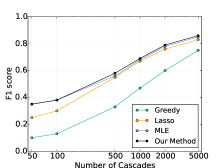
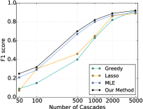
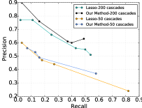
(a) Barabasi-Albert (F$1$ vs. $n$)	(b) Watts-Strogatz (F$1$ vs. $n$)	(c) Holme-Kim (Prec-Recall)
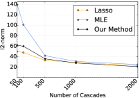
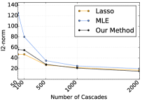
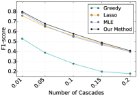
(d) Sparse Kronecker ($\ell_{2}$-norm vs. $n$)	(e) Non-sparse Kronecker ($\ell_{2}$-norm vs. $n$)	(f) Watts-Strogatz (F$1$ vs. $p_{\text{init}}$)

Figure 2: Figures (a) and (b) report the F$1$-score in $\log$ scale for 2 graphs as a function of the number of cascades $n$: (a) Barabasi-Albert graph, $300$ nodes, $16200$ edges. (b) Watts-Strogatz graph, $300$ nodes, $4500$ edges. Figure (c) plots the Precision-Recall curve for various values of $\lambda$ for a Holme-Kim graph ($200$ nodes, $9772$ edges). Figures (d) and (e) report the $\ell_{2}$-norm $\|\hat{\Theta}-\Theta\|_{2}$ for a Kronecker graph which is: (d) exactly sparse (e) non-exactly sparse, as a function of the number of cascades $n$. Figure (f) plots the F$1$-score for the Watts-Strogatz graph as a function of $p_{init}$.

In this section, we validate empirically the results and assumptions of Section 3 for varying levels of sparsity and different initializations of parameters ($n$, $m$, $\lambda$, $p_{\text{init}}$), where $p_{\text{init}}$ is the initial probability of a node being a source node. We compare our algorithm to two different state-of-the-art algorithms: greedy and mle from (Netrapalli & Sanghavi, 2012). As an extra benchmark, we also introduce a new algorithm lasso, which approximates our sparse mle algorithm.

Experimental setup

We evaluate the performance of the algorithms on synthetic graphs, chosen for their similarity to real social networks. We therefore consider a Watts-Strogatz graph ($300$ nodes, $4500$ edges) (Watts & Strogatz, 1998), a Barabasi-Albert graph ($300$ nodes, $16200$ edges) (Albert & Barabási, 2001), a Holme-Kim power law graph ($200$ nodes, $9772$ edges) (Holme & Kim, 2002), and the recently introduced Kronecker graph ($256$ nodes, $10000$ edges) (Leskovec et al., 2010). Undirected graphs are converted to directed graphs by doubling the edges.

For every reported data point, we sample edge weights and generate $n$ cascades from the (IC) model for $n\in\{100,500,1000,2000,5000\}$. We compare for each algorithm the estimated graph $\hat{\cal G}$ with ${\cal G}$. The initial probability of a node being a source is fixed to $0.05$, i.e. an average of $15$ nodes source nodes per cascades for all experiments, except for Figure  (f). All edge weights are chosen uniformly in the interval $[0.2,0.7]$, except when testing for approximately sparse graphs (see paragraph on robustness). Adjusting for the variance of our experiments, all data points are reported with at most a $\pm 1$ error margin. The parameter $\lambda$ is chosen to be of the order ${\cal O}(\sqrt{\log m/(\alpha n)})$. We report our results as a function of the number of cascades and not the number of measurements: in practice, very few cascades have depth greater than 3.

Benchmarks

We compare our sparse mle algorithm to 3 benchmarks: greedy and mle from (Netrapalli & Sanghavi, 2012) and lasso. The mle algorithm is a maximum-likelihood estimator without $\ell_{1}$-norm penalization. greedy is an iterative algorithm. We introduced the lasso algorithm in our experiments to achieve faster computation time:

$$\hat{\theta}_{i}\in\arg\min_{\theta}\sum_{t\in{\cal T}}|f(\theta_{i}\cdot x^{t})-x_{i}^{t+1}|^{2}+\lambda\|\theta_{i}\|_{1}$$

Lasso has the merit of being both easier and faster to optimize numerically than the other convex-optimization based algorithms. It approximates the sparse mle algorithm by making the assumption that the observations $x_{i}^{t+1}$ are of the form: $x_{i}^{t+1}=f(\theta_{i}\cdot x^{t})+\epsilon$, where $\epsilon$ is random white noise. This is not valid in theory since $\epsilon$ depends on $f(\theta_{i}\cdot x^{t})$, however the approximation is validated in practice.

We did not benchmark against other known algorithms (netrate (Gomez-Rodriguez et al., 2011) and first edge (Abrahao et al., 2013)) due to the discrete-time assumption. These algorithms also suppose a single-source model, whereas sparse mle, mle, and greedy do not. Learning the graph in the case of a multi-source cascade model is harder (see Figure 5 (f)) but more realistic, since we rarely have access to “patient 0” in practice.

Graph Estimation

In the case of the lasso, mle and sparse mle algorithms, we construct the edges of $\hat{\cal G}:\cup_{j\in V}\{(i,j):\Theta_{ij}>0.1\}$, i.e by thresholding. Finally, we report the F1-score$=2\text{precision}\cdot\text{recall}/(\text{precision}+\text{recall})$, which considers (1) the number of true edges recovered by the algorithm over the total number of edges returned by the algorithm (precision) and (2) the number of true edges recovered by the algorithm over the total number of edges it should have recovered (recall). Over all experiments, sparse mle achieves higher rates of precision, recall, and F1-score. Interestingly, both mle and sparse mle perform exceptionally well on the Watts-Strogatz graph.

Quantifying robustness

The previous experiments only considered graphs with strong edges. To test the algorithms in the approximately sparse case, we add sparse edges to the previous graphs according to a bernoulli variable of parameter $1/3$ for every non-edge, and drawing a weight uniformly from $[0,0.1]$. The non-sparse case is compared to the sparse case in Figure 5 (d)–(e) for the $\ell_{2}$ norm showing that both the lasso, followed by sparse mle are the most robust to noise.

6 Future Work

Solving the Graph Inference problem with sparse recovery techniques opens new venues for future work. Firstly, the sparse recovery literature has already studied regularization patterns beyond the $\ell_{1}$-norm, notably the thresholded and adaptive lasso (van de Geer et al., 2011; Zou, 2006). Another goal would be to obtain confidence intervals for our estimator, similarly to what has been obtained for the Lasso in the recent series of papers (Javanmard & Montanari, 2014; Zhang & Zhang, 2014).

Finally, the linear threshold model is a commonly studied diffusion process and can also be cast as a generalized linear cascade with inverse link function $z\mapsto\mathbbm{1}_{z>0}$: $X^{t+1}_{j}=\text{sign}\left(\theta_{j}\cdot X^{t}-t_{j}\right)$. This model therefore falls into the 1-bit compressed sensing framework (Boufounos & Baraniuk, 2008). Several recent papers study the theoretical guarantees obtained for 1-bit compressed sensing with specific measurements (Gupta et al., 2010; Plan & Vershynin, 2014). Whilst they obtained bounds of the order ${\cal O}(s\log\frac{m}{s}$), no current theory exists for recovering positive bounded signals from binary measurememts. This research direction may provide the first clues to solve the “adaptive learning” problem: if we are allowed to adaptively choose the source nodes at the beginning of each cascade, how much can we improve the current results?

7 Appendix

In this appendix, we provide the missing proofs of Section 3 and Section 4. We also show additional experiments on the running time of our recovery algorithm which could not fit in the main part of the paper.

7.1 Proofs of Section 3

Proof of Lemma 1.

Using the inequality $\forall x>0,\;\log x\geq 1-\frac{1}{x}$, we have $|\log(\frac{1}{1-p})-\log(\frac{1}{1-p^{\prime}})|\geq\max(1-\frac{1-p}{1-p^{\prime}},1-\frac{1-p^{\prime}}{1-p})\geq\max(p-p^{\prime},p^{\prime}-p)$. ∎

Proof of Lemma 3.

The gradient of $\mathcal{L}$ is given by:

$$\nabla\mathcal{L}(\theta^{*})=\frac{1}{|\mathcal{T}|}\sum_{t\in\mathcal{T}}x^{t}\bigg{[}x_{i}^{t+1}\frac{f^{\prime}}{f}(\theta^{*}\cdot x^{t})\\ -(1-x_{i}^{t+1})\frac{f^{\prime}}{1-f}(\theta^{*}\cdot x^{t})\bigg{]}$$

Let $\partial_{j}\mathcal{L}(\theta)$ be the $j$-th coordinate of $\nabla\mathcal{L}(\theta^{*})$. Writing $\partial_{j}\mathcal{L}(\theta^{*})=\frac{1}{|\mathcal{T}|}\sum_{t\in\mathcal{T}}Y_{t}$ and since $\operatorname{\mathbb{E}}[x_{i}^{t+1}|x^{t}]=f(\theta^{*}\cdot x^{t})$, we have that $\operatorname{\mathbb{E}}[Y_{t+1}|Y_{t}]=0$. Hence $Z_{t}=\sum_{k=1}^{t}Y_{k}$ is a martingale.

Using assumption (LF), we have almost surely $|Z_{t+1}-Z_{t}|\leq\frac{1}{\alpha}$ and we can apply Azuma’s inequality to $Z_{t}$:

$$\operatorname{\mathbb{P}}\big{[}|Z_{\mathcal{T}}|\geq\lambda\big{]}\leq 2\exp\left(\frac{-\lambda^{2}\alpha}{2n}\right)$$

Applying a union bound to have the previous inequality hold for all coordinates of $\nabla\mathcal{L}(\theta)$ implies:

$$\operatorname{\mathbb{P}}\big{[}\|\nabla\mathcal{L}(\theta^{*})\|_{\infty}\geq\lambda\big{]} \leq 2m\exp\left(\frac{-\lambda^{2}n\alpha}{2}\right)$$

Choosing $\lambda\equiv 2\sqrt{\frac{\log m}{\alpha n^{1-\delta}}}$ concludes the proof. ∎

Proof of Corollary 1.

By choosing $\delta=0$, if $n>\frac{9s\log m}{\alpha\gamma^{2}\epsilon^{2}}$, then $\|\hat{\theta}-\theta^{*}\|_{2}<\epsilon<\eta$ with probability $1-\frac{1}{m}$. If $\theta_{i}^{*}=0$ and $\hat{\theta}>\eta$, then $\|\hat{\theta}-\theta^{*}\|_{2}\geq|\hat{\theta}_{i}-\theta_{i}^{*}|>\eta$, which is a contradiction. Therefore we get no false positives. If $\theta_{i}^{*}>\eta+\epsilon$, then $|\hat{\theta}_{i}-\theta_{i}^{*}|<\epsilon\implies\theta_{j}>\eta$ and we get all strong parents. ∎

(RE) with high probability

We now prove Proposition 1. The proof mostly relies on showing that the Hessian of likelihood function $\mathcal{L}$ is sufficiently well concentrated around its expectation.

Proof.

Writing $H\equiv\nabla^{2}\mathcal{L}(\theta^{*})$, if $\forall\Delta\in C(S),\;\|\operatorname{\mathbb{E}}[H]-H]\|_{\infty}\leq\lambda$ and $\operatorname{\mathbb{E}}[H]$ verifies the $(S,\gamma)$-(RE) condition then:

$$\forall\Delta\in C(S),\;\Delta H\Delta\geq\Delta\operatorname{\mathbb{E}}[H]\Delta(1-32s\lambda/\gamma)$$ (6)

Indeed, $|\Delta(H-E[H])\Delta|\leq 2\lambda\|\Delta\|_{1}^{2}\leq 2\lambda(4\sqrt{s}\|\Delta_{s}\|_{2})^{2}$. Writing $\partial^{2}_{i,j}\mathcal{L}(\theta^{*})=\frac{1}{|\mathcal{T}|}\sum_{t\in T}Y_{t}$ and using $(LF)$ and $(LF2)$ we have $\big{|}Y_{t}-\operatorname{\mathbb{E}}[Y_{t}]\big{|}\leq\frac{3}{\alpha}$. Applying Azuma’s inequality as in the proof of Lemma 3, this implies:

$$\operatorname{\mathbb{P}}\big{[}\|\operatorname{\mathbb{E}}[H]-H\|_{\infty}\geq\lambda\big{]}\leq 2\exp\left(-\frac{n\alpha\lambda^{2}}{3}+2\log m\right)$$

Thus, if we take $\lambda=\sqrt{\frac{9logm}{\alpha n^{1-\delta}}}$, $\|E[H]-H\|_{\infty}\leq\lambda$ w.p at least $1-e^{-n^{\delta}\log m}$. When $n^{1-\delta}\geq\frac{1}{28\gamma\alpha}s^{2}\log m$, (6) implies $\forall\Delta\in C(S),\;\Delta H\Delta\geq\frac{1}{2}\Delta\operatorname{\mathbb{E}}[H]\Delta,$ w.p. at least $1-e^{-n^{\delta}\log m}$ and the conclusion of Proposition 1 follows. ∎

7.2 Proof of Theorem 3

Let us consider an algorithm $\mathcal{A}$ which verifies the recovery guarantee of Theorem 3: there exists a probability distribution over measurements such that for all vectors $\theta^{*}$, (5) holds w.p. $\delta$. This implies by the probabilistic method that for all distribution $D$ over vectors $\theta$, there exists an $n\times m$ measurement matrix $X_{D}$ with such that (5) holds w.p. $\delta$ ($\theta$ is now the random variable).

Consider the following distribution $D$: choose $S$ uniformly at random from a “well-chosen” set of $s$-sparse supports $\mathcal{F}$ and $t$ uniformly at random from $X\equiv\big{\{}t\in\{-1,0,1\}^{m}\,|\,\mathrm{supp}(t)\in\mathcal{F}\big{\}}$. Define $\theta=t+w$ where $w\sim\mathcal{N}(0,\alpha\frac{s}{m}I_{m})$ and $\alpha=\Omega(\frac{1}{C})$.

Consider the following communication game between Alice and Bob: (1) Alice sends $y\in\mathbb{R}^{m}$ drawn from a Bernouilli distribution of parameter $f(X_{D}\theta)$ to Bob. (2) Bob uses $\mathcal{A}$ to recover $\hat{\theta}$ from $y$. It can be shown that at the end of the game Bob now has a quantity of information $\Omega(s\log\frac{m}{s})$ about $S$. By the Shannon-Hartley theorem, this information is also upper-bounded by $\mathcal{O}(n\log C)$. These two bounds together imply the theorem.

7.3 Running Time Analysis

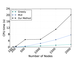
Figure 3: Running time analysis for estimating the parents of a single node on a Barabasi-Albert graph as a function of the number of nodes in the graph. The parameter $k$ (number of nodes each new node is attached to) was set to $30$. $p_{\text{init}}$ is chosen equal to $.15$, and the edge weights are chosen uniformly at random in $[.2,.7]$. The penalization parameter $\lambda$ is chosen equal to $.1$.

Figure 4: Running time analysis for estimating the parents of a single node on a Barabasi-Albert graph as a function of the number of total observed cascades. The parameters defining the graph were set as in Figure 3.

We include here a running time analysis of our algorithm. In Figure 3, we compared our algorithm to the benchmark algorithms for increasing values of the number of nodes. In Figure 4, we compared our algorithm to the benchmarks for a fixed graph but for increasing number of observed cascades.

In both Figures, unsurprisingly, the simple greedy algorithm is the fastest. Even though both the MLE algorithm and the algorithm we introduced are based on convex optimization, the MLE algorithm is faster. This is due to the overhead caused by the $\ell_{1}$-regularisation in (2).

The dependency of the running time on the number of cascades increases is linear, as expected. The slope is largest for our algorithm, which is again caused by the overhead induced by the $\ell_{1}$-regularization.

References

- Abrahao et al. (2013) Abrahao, Bruno D., Chierichetti, Flavio, Kleinberg, Robert, and Panconesi, Alessandro. Trace complexity of network inference. In The 19th ACM SIGKDD International Conference on Knowledge Discovery and Data Mining, KDD 2013, Chicago, IL, USA, August 11-14, 2013, pp. 491–499, 2013.
- Adar & Adamic (2005) Adar, Eytan and Adamic, Lada A. Tracking information epidemics in blogspace. In 2005 IEEE / WIC / ACM International Conference on Web Intelligence (WI 2005), 19-22 September 2005, Compiegne, France, pp. 207–214, 2005.
- Albert & Barabási (2001) Albert, Réka and Barabási, Albert-László. Statistical mechanics of complex networks. CoRR, cond-mat/0106096, 2001.
- Ba et al. (2011) Ba, Khanh Do, Indyk, Piotr, Price, Eric, and Woodruff, David P. Lower bounds for sparse recovery. CoRR, abs/1106.0365, 2011.
- Bickel et al. (2009a) Bickel, Peter J, Ritov, Ya’acov, and Tsybakov, Alexandre B. Simultaneous analysis of lasso and dantzig selector. The Annals of Statistics, pp. 1705–1732, 2009a.
- Bickel et al. (2009b) Bickel, Peter J., Ritov, Ya’acov, and Tsybakov, Alexandre B. Simultaneous analysis of lasso and dantzig selector. Ann. Statist., 37(4):1705–1732, 08 2009b.
- Boufounos & Baraniuk (2008) Boufounos, Petros and Baraniuk, Richard G. 1-bit compressive sensing. In 42nd Annual Conference on Information Sciences and Systems, CISS 2008, Princeton, NJ, USA, 19-21 March 2008, pp. 16–21, 2008.
- Candes & Tao (2006) Candes, Emmanuel J and Tao, Terence. Near-optimal signal recovery from random projections: Universal encoding strategies? Information Theory, IEEE Transactions on, 52(12):5406–5425, 2006.
- Daneshmand et al. (2014) Daneshmand, Hadi, Gomez-Rodriguez, Manuel, Song, Le, and Schölkopf, Bernhard. Estimating diffusion network structures: Recovery conditions, sample complexity & soft-thresholding algorithm. In Proceedings of the 31th International Conference on Machine Learning, ICML 2014, Beijing, China, 21-26 June 2014, pp. 793–801, 2014.
- Donoho (2006) Donoho, David L. Compressed sensing. Information Theory, IEEE Transactions on, 52(4):1289–1306, 2006.
- Du et al. (2013) Du, Nan, Song, Le, Woo, Hyenkyun, and Zha, Hongyuan. Uncover topic-sensitive information diffusion networks. In Proceedings of the Sixteenth International Conference on Artificial Intelligence and Statistics, pp. 229–237, 2013.
- Du et al. (2014) Du, Nan, Liang, Yingyu, Balcan, Maria, and Song, Le. Influence function learning in information diffusion networks. In Proceedings of the 31st International Conference on Machine Learning (ICML-14), pp. 2016–2024, 2014.
- Gomez Rodriguez et al. (2010) Gomez Rodriguez, Manuel, Leskovec, Jure, and Krause, Andreas. Inferring networks of diffusion and influence. In Proceedings of the 16th ACM SIGKDD International Conference on Knowledge Discovery and Data Mining, KDD ’10, pp. 1019–1028, New York, NY, USA, 2010. ACM. ISBN 978-1-4503-0055-1.
- Gomez-Rodriguez et al. (2011) Gomez-Rodriguez, Manuel, Balduzzi, David, and Schölkopf, Bernhard. Uncovering the temporal dynamics of diffusion networks. CoRR, abs/1105.0697, 2011.
- Gupta et al. (2010) Gupta, Ankit, Nowak, Robert, and Recht, Benjamin. Sample complexity for 1-bit compressed sensing and sparse classification. In IEEE International Symposium on Information Theory, ISIT 2010, June 13-18, 2010, Austin, Texas, USA, Proceedings, pp. 1553–1557, 2010.
- Holme & Kim (2002) Holme, Petter and Kim, Beom Jun. Growing scale-free networks with tunable clustering. Physical review E, 65:026–107, 2002.
- Javanmard & Montanari (2014) Javanmard, Adel and Montanari, Andrea. Confidence intervals and hypothesis testing for high-dimensional regression. The Journal of Machine Learning Research, 15(1):2869–2909, 2014.
- Kempe et al. (2003) Kempe, David, Kleinberg, Jon M., and Tardos, Éva. Maximizing the spread of influence through a social network. In Proceedings of the Ninth ACM SIGKDD International Conference on Knowledge Discovery and Data Mining, Washington, DC, USA, August 24 - 27, 2003, pp. 137–146, 2003.
- Leskovec et al. (2007) Leskovec, Jure, McGlohon, Mary, Faloutsos, Christos, Glance, Natalie S., and Hurst, Matthew. Patterns of cascading behavior in large blog graphs. In Proceedings of the Seventh SIAM International Conference on Data Mining, April 26-28, 2007, Minneapolis, Minnesota, USA, pp. 551–556, 2007.
- Leskovec et al. (2010) Leskovec, Jure, Chakrabarti, Deepayan, Kleinberg, Jon M., Faloutsos, Christos, and Ghahramani, Zoubin. Kronecker graphs: An approach to modeling networks. Journal of Machine Learning Research, 11:985–1042, 2010.
- Liben-Nowell & Kleinberg (2008) Liben-Nowell, David and Kleinberg, Jon. Tracing information flow on a global scale using Internet chain-letter data. Proceedings of the National Academy of Sciences, 105(12):4633–4638, 2008.
- Negahban et al. (2012) Negahban, Sahand N., Ravikumar, Pradeep, Wrainwright, Martin J., and Yu, Bin. A unified framework for high-dimensional analysis of m-estimators with decomposable regularizers. Statistical Science, 27(4):538–557, December 2012.
- Netrapalli & Sanghavi (2012) Netrapalli, Praneeth and Sanghavi, Sujay. Learning the graph of epidemic cascades. SIGMETRICS Perform. Eval. Rev., 40(1), June 2012. ISSN 0163-5999.
- Plan & Vershynin (2014) Plan, Yaniv and Vershynin, Roman. Dimension reduction by random hyperplane tessellations. Discrete & Computational Geometry, 51(2):438–461, 2014.
- Price & Woodruff (2011) Price, Eric and Woodruff, David P. (1 + eps)-approximate sparse recovery. In Ostrovsky, Rafail (ed.), IEEE 52nd Annual Symposium on Foundations of Computer Science, FOCS 2011, Palm Springs, CA, USA, October 22-25, 2011, pp. 295–304. IEEE Computer Society, 2011. ISBN 978-1-4577-1843-4.
- Price & Woodruff (2012) Price, Eric and Woodruff, David P. Applications of the shannon-hartley theorem to data streams and sparse recovery. In Proceedings of the 2012 IEEE International Symposium on Information Theory, ISIT 2012, Cambridge, MA, USA, July 1-6, 2012, pp. 2446–2450. IEEE, 2012. ISBN 978-1-4673-2580-6.
- Raskutti et al. (2010) Raskutti, Garvesh, Wainwright, Martin J., and Yu, Bin. Restricted eigenvalue properties for correlated gaussian designs. Journal of Machine Learning Research, 11:2241–2259, 2010.
- Rudelson & Zhou (2013) Rudelson, Mark and Zhou, Shuheng. Reconstruction from anisotropic random measurements. IEEE Transactions on Information Theory, 59(6):3434–3447, 2013.
- van de Geer et al. (2011) van de Geer, Sara, Bühlmann, Peter, and Zhou, Shuheng. The adaptive and the thresholded lasso for potentially misspecified models (and a lower bound for the lasso). Electron. J. Statist., 5:688–749, 2011.
- van de Geer & Bühlmann (2009) van de Geer, Sara A. and Bühlmann, Peter. On the conditions used to prove oracle results for the lasso. Electron. J. Statist., 3:1360–1392, 2009.
- Watts & Strogatz (1998) Watts, Duncan J. and Strogatz, Steven H. Collective dynamics of ‘small-world’ networks. Nature, 393(6684):440–442, 1998.
- Zhang & Zhang (2014) Zhang, Cun-Hui and Zhang, Stephanie S. Confidence intervals for low dimensional parameters in high dimensional linear models. Journal of the Royal Statistical Society: Series B (Statistical Methodology), 76(1):217–242, 2014.
- Zhao & Yu (2006) Zhao, Peng and Yu, Bin. On model selection consistency of lasso. J. Mach. Learn. Res., 7:2541–2563, December 2006. ISSN 1532-4435.
- Zou (2006) Zou, Hui. The adaptive lasso and its oracle properties. Journal of the American Statistical Association, 101(476):1418–1429, 2006.