Angular momentum transport and large eddy simulations in magnetorotational turbulence: the small Pm limit.

Abstract

Context. Angular momentum transport in accretion discs is often believed to be due to magnetohydrodynamic turbulence mediated by the magnetorotational instability (MRI). Despite an abundant literature on the MRI, the parameters governing the saturation amplitude of the turbulence are poorly understood and the existence of an asymptotic behavior in the Ohmic diffusion regime is not clearly established.

Aims. We investigate the properties of the turbulent state in the small magnetic Prandtl number limit. Since this is extremely computationally expensive, we also study the relevance and range of applicability of the most common subgrid scale models for this problem.

Methods. Unstratified shearing boxes simulations are performed both in the compressible and incompressible limits, with a resolution up to 800 cells per disc scale height. The latter constitutes the largest resolution ever attained for a simulation of MRI turbulence. Different magnetic field geometry and a large range of dimensionless dissipative coefficients are considered. We also systematically investigate the interest of using large eddy simulations (LES).

Results. In the presence of a mean magnetic field threading the domain, angular momentum transport converges to a finite value in the small $Pm$ limit. When the mean vertical field amplitude is such that $\beta$, the ratio between the thermal and magnetic pressure, equals $10^{3}$, we find $\alpha\sim 3.2\times 10^{-2}$ when $Pm$ approaches zero. In the case of a mean toroidal field for which $\beta=100$, we find $\alpha\sim 1.8\times 10^{-2}$ in the same limit. Both implicit LES and Chollet-Lesieur closure model reproduces these results for the $\alpha$ parameter and the power spectra. A reduction in computational cost of a factor at least $16$ (and up to $256$) is achieved when using such methods.

Conclusions. MRI turbulence operates efficiently in the small Pm limit provided there is a mean magnetic field. Implicit LES offers a practical and efficient mean of investigation of this regime but should be used with care, particularly in the case of a vertical field. Chollet-Lesieur closure model is perfectly suited for simulations done with a spectral code.

1 Introduction

Determining the rate of angular momentum transport in accretion discs is considered as one of the key unsolved astrophysical questions. Accretion is believed to be at the origin of the radiation emitted by some of the most luminous sources in the universe from active galactic nuclei to X-ray binaries and is also a major process at work during planet formation in protoplanetary discs (Frank et al., 2002). In addition, accretion discs are ubiquitous in the universe and affect the dynamics, evolution and appearance of multiple astrophysical objects at all spatial and energy scales. The accretion rate can be indirectly constrained by the luminosity of high-energy sources or the life-time of protoplanetary discs, and, if the transport process is modeled by an $\alpha$ viscosity (Shakura & Sunyaev, 1973), such an estimate gives $0.01<\alpha<0.4$ depending on the system considered (King et al., 2007).

The physical origin of angular momentum transport has to be understood to explain such an efficient radial angular momentum transport. Currently, the most widely accepted mechanism is magnetohydrodynamic (MHD) turbulence induced by the non-linear evolution of the magneto-rotational instability (MRI, Balbus & Hawley, 1991). That instability along with its nonlinear development has been extensively studied in the last two decades (Balbus & Hawley, 1998; Balbus, 2003; Fromang, 2013). Using local simulations performed in the framework of the shearing box, Hawley et al. (1995) quickly established that the MRI develops into vigorous MHD turbulence that efficiently transports angular momentum outward, a result that was later confirmed to be independent of the field geometry (Hawley et al., 1996) or to the background disc stratification (Brandenburg et al., 1995; Stone et al., 1996). Only recently the sensitivity of MRI–driven MHD turbulence saturation to small scale dissipation in such idealized simulations has been identified: when magnetic field diffusion is dominated by an ohmic resistivity $\eta$, $\alpha$ is an increasing function of the magnetic Prandtl number $Pm$, the ratio between the kinematic viscosity $\nu$ and $\eta$. This is the case both in the presence of a mean vertical magnetic field (Lesur & Longaretti, 2007) and of a mean azimuthal magnetic field (Simon & Hawley, 2009). Such a “Pm–effect” has a significant impact on the rate of angular momentum transport measured in homogeneous shearing boxes simulations: in the case of a mean vertical field such that the plasma $\beta$ parameter (defined in section 2.4) amounts to $10^{3}$, Longaretti & Lesur (2010) showed that $\alpha$ varies by a factor of about $5$ when $Pm$ only varies between $1/4$ and $4$, without any sign of the relation flattening at either range. The dynamo case (i.e. no mean magnetic field threading the computational domain) also displays a large sensitivity to $Pm$ (Fromang et al., 2007; Simon & Hawley, 2009; Guan et al., 2009; Bodo et al., 2011) that persists when density stratification is included (Simon et al., 2011). In this dynamo regime and without stratification, the effect is even stronger and dynamo action is suppressed for $Pm$ values smaller than unity, in which case the flow remains laminar, i.e. $\alpha$ goes to zero. A clear understanding of the origin of the effect of $Pm$ on the rate of angular momentum transport is still lacking and is currently a matter of active research. The first results, based on methods borrowed from the fluid community (Herault et al., 2011; Riols et al., 2013) are promising (Riols et al., 2015) and should be extended to more realistic geometries and dimensionless numbers.

Taken together, the results described above question the relevance of MRI–driven MHD turbulence as the dominant transport mechanism in accretion discs where the Prandtl number can be orders of magnitude lower ($Pm\ll 1$) than has been explored in published simulations (Balbus & Henri, 2008). There is clearly the possibility that $\alpha$ becomes vanishingly small as $Pm$ decreases to small, but astrophysically relevant values. The first goal of this paper is to investigate that asymptotic behavior by means of high resolution simulations performed in the homogeneous shearing box. In doing so, we will leave aside the dynamo case and focus on vertical and azimuthal mean field configurations. Using high resolution simulations (such that the coverage in $Pm$ now extends over more than two orders of magnitudes, from $10^{-2}$ to $4$), we will show that $\alpha$ asymptotically converges to a well defined finite value in both cases. However, the computational cost associated with such simulations is extremely large (for example, $15$ millions CPU hours are needed to complete the $1000^{3}$ simulation we describe in section 3.1.1 on a BlueGen/Q machine ranked $42$nd on the Top500 supercomputing website in november 2014 ). In practice, such a large cost is prohibitive if one wants to perform a parameter survey in the asymptotic regime with additional physics included and simply prevents global simulations to be performed in that limit. The second goal of this paper is thus to investigate the possibility to use sub–grid scale models as a mean to reduce the computational cost associated with MHD turbulence simulations in the small $Pm$ limit.

Recent years have seen significant progress in our understanding of the consequences of ambipolar diffusion (Bai & Stone, 2011, 2013; Simon et al., 2013) and the Hall effect (Kunz & Lesur, 2013; Lesur et al., 2014; Bai, 2015), both of which are particularly important in shaping the structure of protoplanetary discs. In this paper we will restrict our attention to Ohmic resistivity as the sole source of magnetic field dissipation. Such a regime is relevant to describe the very inner parts of protoplanetary discs (at stellar distances of a few tens of an AU) but also cataclysmic variables (CV) discs and the outer parts of X-ray binaries discs (Balbus & Henri, 2008). In principle, the analysis we present here should also be carried for such cases where ambipolar diffusion or the Hall effect are the dominant magnetic field diffusion processes.

The plan of the paper is as follows. In the following section, the equations and numerical methods are given. Section 3 presents our results, focusing first on simulations that explicitly resolve the small dissipative scales (section 3.1) and then on two different methods to perform Large Eddy Simulations (LES) in section 3.2. We finally conclude and discuss the implications of our work in section 4.

2 Methods

2.1 Equations and notations

In this paper, we use the shearing box approximation (Hawley et al., 1995). Namely, we compute the evolution of the fluid in a small box centered at a radius $r_{0}$ of the disc and rotating at the same velocity as the fluid at $r=r_{0}$. As the size of the box is small compared to the radial position, the curvature terms of the standard fluid equations can be simplified (Hawley & Balbus, 1992). We thus use Cartesian coordinates $(x,y,z)$ with units vectors ($\@vec{i},\@vec{j},\@vec{k}$). In this coordinate system, we note $(L_{x},L_{y},L_{z})$ the size of the computational box. Neglecting the vertical component of the gravitational acceleration, we solve the following set of equations:

$$\partial_{t}\rho+\@vec{\nabla}\cdot(\rho\@vec{v}) = 0$$ (1)

$$\partial_{t}(\rho\@vec{v})+\@vec{\nabla}\cdot(\rho\@vec{v}\@vec{v}-\@vec{B}\@vec{B})+\@vec{\nabla}P_{tot} = 2q\rho\Omega_{0}^{2}x\@vec{i}-2\rho\@vec{\Omega}_{0}\times\@vec{v}$$

$$+\@vec{\nabla}\cdot\@vec{T}$$ (2)

$$\partial_{t}\@vec{B} = \@vec{\nabla}\times(\@vec{v}\times\@vec{B}-\eta\@vec{\nabla}\times\@vec{B})$$ (3)

where $\rho$ is the fluid density, $\@vec{v}$ its velocity in the rotating frame, $\@vec{B}$ is the magnetic field and $\Omega_{0}$ is the angular velocity of the fluid at $r_{0}$, corresponding to the angular velocity of the box. $q$ stands for the background keplerian shear and is taken equal to $1.5$ throughout this paper. $P_{tot}$ is the total pressure, the sum of the thermal pressure $P$ and the magnetic pressure $B^{2}/2$. Explicit dissipation is accounted for through the Ohmic resistivity $\eta$ and the kinematic viscosity $\nu$ that enters in the viscous stress tensor $T$ defined as

$$T_{ij}=\rho\nu\left(\partial_{j}v_{i}+\partial_{i}v_{j}-\frac{2}{3}\delta_{ij}\@vec{\nabla}\cdot\@vec{v}\right)\,.$$ (4)

The amplitude of viscosity and resistivity are set using the magnitude of the Reynolds number $Re$ and magnetic Reynolds number $Rm$ with the following relations

$$Re=\frac{\Omega_{0}L_{z}^{2}}{\nu}\,,Rm=\frac{\Omega_{0}L_{z}^{2}}{\eta}$$

which can also serve as an alternative definition for the magnetic Prandtl number $Pm$ already given in the introduction:

$$Pm=\frac{\nu}{\eta}=\frac{Rm}{Re}\,.$$ (5)

We performed simulations that consider two different flavors of the system of equations (1), (2) and (3). First, we solve the above equations in the incompressible limit. In this case, the density is constant and equation (1) reduces to $\mbox{\boldmath{$\nabla$}}\mbox{\boldmath{$\cdot$}}\mbox{\boldmath{$v$}}=0$. We used the code SNOOPY in that case (see section 2.2). In the second type of simulations, we solve the full set of equations (and refer to that case as the compressible simulations) using the code RAMSES (section 2.3). We briefly describe below the two codes and the specificities of each set of simulations.

2.2 Incompressible simulations: the SNOOPY code

The SNOOPY code is a pseudo spectral code that solves the incompressible MHD equations in a Fourier basis. It uses a low-storage 3^rd order Runge-Kutta integrator and works in a sheared frame comoving with the mean flow, which is equivalent to a 3^rd order Fargo scheme (Masset, 2000). SNOOPY uses a $3/2$ antialiasing rule to eliminate the excitation of spurious modes during the computation of quadratic nonlinearities.

The use of a sheared Fourier basis makes the boundary conditions periodic in the $y$ and $z$ directions and shear-periodic in the $x$ direction. SNOOPY conserves linear momentum and magnetic flux down to machine precision. Since spectral methods are inherently diffusion-free and energy conserving, the addition of dissipation is required to mimic the damping due to small scale dissipation processes. In SNOOPY, one can choose second order diffusion operators, hyperdiffusion operators or Chollet & Lesieur (1981) subgrid models (see section 3.2.1).

2.3 Compressible simulations: the RAMSES code

The RAMSES code is a finite volume code that solves the compressible MHD equations on a Cartesian grid (Teyssier, 2002; Fromang et al., 2006) using the constrained transport algorithm (Evans & Hawley, 1988). We use a version of the code for which the grid is uniform (i.e. without the adaptive mesh refinement). The source terms associated with the tidal potential are included as described by Stone & Gardiner (2010). We use the HLLD Riemann solver (Miyoshi & Kusano, 2005) with monotonized central slope limiter, shearing box boundary conditions in the $x$ direction (Hawley et al., 1995) and periodic boundary conditions in the $y$ and $z$ directions. For extended box sizes such as used in the mean vertical field case (see section 2.4), it has been found that radially variable numerical dissipation causes the turbulent stress to vary accross the box. To avoid that problem, we used the FARGO algorithm (Masset, 2000; Stone & Gardiner, 2010) in that case, which also improves the efficiency of the code through an increase in the timestep.

Throughout this paper, we use an isothermal equation of state to close the system of MHD equations in compressible simulations, such that $P=\rho c_{0}^{2}$, where $c_{0}$ stands for the constant sound speed. We start the simulation with an initial uniform density $\rho=\rho_{0}$ and choose $L_{z}=H=c_{0}/\Omega_{0}$ where $H$ is the disc scale height.

2.4 Models parameters

We start the simulations with a uniform initial magnetic field:

$$\mbox{\boldmath{$B$}}=B_{0y}\mbox{\boldmath{$j$}}+B_{0z}\mbox{\boldmath{$k$}}\,.$$ (6)

Two different initial magnetic configurations are considered in the following, namely pure azimuthal field ($B_{0z}=0$) simulations and pure vertical field simulations ($B_{0y}=0$). The strength of the magnetic field is defined using the plasma parameter $\beta_{i}$ that is given by

$$\beta_{i}\equiv\left\{\begin{array}[]{l l}\frac{q^{2}\rho_{0}c_{0}^{2}}{B_{0i}^{2}}&\quad\text{in compressible runs,}\\ \frac{(q\Omega L_{z})^{2}}{B_{0i}^{2}}&\quad\text{in incompressible runs.}\\ \end{array}\right.$$ (9)

For the mean azimuthal (resp. vertical) magnetic field simulations, we used $\beta_{y}=112.5$ (resp. $\beta_{z}=10^{3}$). At the start of each runs, small amplitude random velocity perturbations are added on the three velocity components with an amplitude equal to $1\%$ of the sound speed in compressible runs. In incompressible simulations both velocity and magnetic random perturbations are added with an amplitude of $0.1\Omega L_{z}$.

The size of the computational box is either $(L_{z},4L_{z},L_{z})$ for the simulations with a mean azimuthal magnetic field, or $(4L_{z},4L_{z},L_{z})$ for the simulations with a mean vertical magnetic field. In the latter case, it is indeed well known that boxes with $L_{x}=L_{z}$ artificially enhance the importance of recurrent bursts in the flow structure (Bodo et al., 2008; Johansen et al., 2009). In such box sizes and with such vertical magnetic field, Bai & Stone (2014) recently reported zonal flows. We also found such structures in our simulations.

The resolution varies from $32$ cells per unit length up to $800$ cells per unit length. Such large resolutions allow us to reach the largest Reynolds number (run Y-C-Re85000, $Re=85000$) and the smallest Prandtl number (run Z-I-Re40000, $Pm=0.01$) ever published. As larger structures are expected in the $y$-direction, we typically use a resolution that is twice as coarse in that direction.

3 Results

Model	Resolution	TRun	Re	Rm	Pm	$\alpha$	$\alpha_{Max}$	$\alpha_{Rey}$	$R$
Y-C-Re650	$(64,128,64)$	100	650	2600	4	$3.0\times 10^{-2}$	$2.4\times 10^{-2}$	$5.9\times 10^{-3}$	$4.2$
Y-C-Re2600	$(64,128,64)$	100	2600	2600	1	$2.5\times 10^{-2}$	$1.9\times 10^{-2}$	$5.7\times 10^{-3}$	$3.4$
Y-C-Re13000	$(128,256,128)$	100	13000	2600	0.2	$1.8\times 10^{-2}$	$1.4\times 10^{-2}$	$4.6\times 10^{-3}$	$3.0$
Y-C-Re26000	$(256,512,256)$	100	26000	2600	0.1	$2.0\times 10^{-2}$	$1.5\times 10^{-2}$	$5.0\times 10^{-3}$	$3.0$
Y-C-Re85000	$(800,1600,832)$	35	85000	2600	0.03	$1.8\times 10^{-2}$	$1.3\times 10^{-2}$	$4.6\times 10^{-3}$	$2.9$
Y-ILES-C-64	$(64,128,64)$	100	-	2600	-	$1.9\times 10^{-2}$	$1.4\times 10^{-2}$	$4.7\times 10^{-2}$	$3.0$
Y-ILES-C-128	$(128,256,128)$	100	-	2600	-	$1.9\times 10^{-2}$	$1.4\times 10^{-2}$	$4.8\times 10^{-3}$	$3.0$
Y-ILES-C-256	$(256,512,256)$	100	-	2600	-	$1.9\times 10^{-2}$	$1.4\times 10^{-2}$	$5.0\times 10^{-3}$	$2.8$

Table 1: RAMSES runs with a mean azimuthal field. The box size is $(L_{x},L_{y},L_{z})=(L_{z},4L_{z},L_{z})$. $T_{run}$ is given in local orbits time units. The table gives for each run its resolution, duration, Reynolds number, magnetic Reynolds number, magnetic Prandtl number, total stress, Maxwell stress, Reynolds stress and the ratio of the two.

Model	Resolution	TRun	Re	Rm	Pm	$\alpha$	$\alpha_{Max}$	$\alpha_{Rey}$	$R$
Z-C-Re400	$(128,64,32)$	100	400	400	1	$6.5\times 10^{-2}$	$4.0\times 10^{-2}$	$2.4\times 10^{-2}$	$1.6$
Z-C-Re800	$(256,128,64)$	100	800	400	0.5	$5.1\times 10^{-2}$	$2.9\times 10^{-2}$	$2.2\times 10^{-2}$	$1.3$
Z-C-Re3000	$(512,256,128)$	100	3000	400	0.13	$3.7\times 10^{-2}$	$2.0\times 10^{-2}$	$1.8\times 10^{-2}$	$1.1$
Z-C-Re8000	$(1024,512,256)$	100	8000	400	0.05	$3.1\times 10^{-2}$	$1.5\times 10^{-2}$	$1.6\times 10^{-2}$	$1.0$
Z-ILES-C-32	$(128,64,32)$	100	-	400	-	$4.1\times 10^{-2}$	$2.2\times 10^{-2}$	$1.9\times 10^{-2}$	$1.2$
Z-ILES-C-64	$(256,128,64)$	100	-	400	-	$3.6\times 10^{-2}$	$1.8\times 10^{-2}$	$1.8\times 10^{-2}$	$1.0$
Z-ILES-C-128	$(512,256,128)$	100	-	400	-	$3.3\times 10^{-2}$	$1.6\times 10^{-2}$	$1.7\times 10^{-2}$	$1.0$
Z-ILES-C-256*	$(1024,512,256)$	40	-	400	-	$3.3\times 10^{-2}$	$1.6\times 10^{-2}$	$1.8\times 10^{-2}$	$0.9$

Table 2: Same than table 1 but for RAMSES runs with a mean vertical field. The box size is $(L_{x},L_{y},L_{z})=(4L_{z},4L_{z},L_{z})$. *To save computational time, this model was performed by restarting model Z-C-Re8000 at $t=50$ removing explicit viscosity

Model	Resolution	TRun	Re	Rm	Pm	$\alpha$	$\alpha_{Max}$	$\alpha_{Rey}$	$R$
Z-I-Re1300	$(256,256,64)$	$53$	1333	400	0.3	$3.8\times 10^{-2}$	$2.8\times 10^{-2}$	$9.9\times 10^{-3}$	$2.8$
Z-I-Re20000	$(1536,768,192)$	$53$	20000	400	0.02	$3.5\times 10^{-2}$	$2.6\times 10^{-2}$	$9.2\times 10^{-3}$	$2.8$
Z-I-Re40000	$(3072,1536,384)$	$53$	40000	400	0.01	$3.3\times 10^{-2}$	$2.3\times 10^{-2}$	$1.0\times 10^{-2}$	$2.4$
Z-CL-192-a	$(768,384,192)$	$53$	-	400	-	$3.3\times 10^{-2}$	$2.4\times 10^{-2}$	$8.8\times 10^{-3}$	$2.8$
Z-CL-192-b	$(768,384,192)$	$53$	-	400	-	$3.2\times 10^{-2}$	$2.3\times 10^{-2}$	$9.3\times 10^{-3}$	$2.5$
Z-CL-128-a	$(512,256,128)$	$53$	-	400	-	$3.5\times 10^{-2}$	$2.4\times 10^{-2}$	$1.0\times 10^{-2}$	$2.4$
Z-CL-128-b	$(512,256,128)$	$53$	-	400	-	$3.4\times 10^{-2}$	$2.5\times 10^{-2}$	$9.7\times 10^{-3}$	$2.5$
Z-CL-96-a	$(384,192,96)$	$53$	-	400	-	$3.4\times 10^{-2}$	$2.5\times 10^{-2}$	$9.2\times 10^{-3}$	$2.8$
Z-CL-96-b	$(384,192,96)$	$53$	-	400	-	$3.7\times 10^{-2}$	$2.6\times 10^{-2}$	$1.1\times 10^{-2}$	$2.3$

Table 3: Same than table 1 but for SNOOPY runs. All runs have a box size of $(L_{x},L_{y},L_{z})=(4L_{z},4L_{z},L_{z})$.

The whole set of runs discussed in the remaining of this paper is listed in tables 1, 2 and 3, where the first column provides the simulation labels. Runs starting with a pure azimuthal (vertical) magnetic field are labelled with letter “Y” (“Z”). Likewise, compressible (incompressible) simulations are labelled with letter “C” (“I”). Large Eddy Simulations (LES) are labelled either “ILES” or “CL” depending on the subgrid scale model that is used (see section 3.2). The remaining columns in tables 1, 2 and 3 give the run resolution (col. 2) and duration $T_{Run}$ (col. 3), the Reynolds number (col. 4), the magnetic Reynolds number (col. 5), the magnetic Prandtl number (col. 6), and $\alpha$ (col. 7), the sum of $\alpha_{Rey}$ (col. 8) and $\alpha_{Max}$ (col. 9). The later are defined by the following relations:

$$\alpha_{Rey}=\left\{\begin{array}[]{l l}\frac{\langle\rho\delta v_{r}\delta u_{\phi}\rangle}{P_{0}}&\quad\text{in compressible runs,}\\ \frac{\langle\delta v_{r}\delta u_{\phi}\rangle}{(\Omega Lz)^{2}}&\quad\text{in incompressible runs,}\\ \end{array}\right.$$ (13)

$$\alpha_{Max}=\left\{\begin{array}[]{l l}-\frac{\langle B_{r}B_{\phi}\rangle}{P_{0}}&\quad\text{in compressible runs,}\\ -\frac{\langle B_{r}B_{\phi}\rangle}{\rho_{0}(\Omega Lz)^{2}}&\quad\text{in incompressible runs.}\\ \end{array}\right.$$ (16)

Here $\langle.\rangle$ denotes an average over the shearing box volume and over time and $\delta v$ is the velocity difference to the laminar sheared flow. Except for the shortest runs (see for instance section 3.1.1), the turbulent transport rates as measured by the $\alpha$ parameters are time averaged over the last $60$ orbits of the models. The last column finally gives the ratio between magnetic and hydrodynamic transport rate.

3.1 Direct Numerical Simulations (DNS) in the small Pm regime

In this section, we present the results of the resolved simulations (meaning that kinematic viscosity and ohmic resistivity are explicitly included in the calculation), focusing on the rate of angular momentum transport and on the power spectra of the turbulent flow.

3.1.1 A $1000^{3}$ MRI simulation

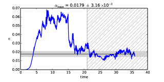
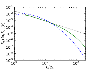
Figure 1: Top panel: Time evolution of $\alpha$ in model Y-C-Re85000 for which $Pm=0.03$. The initial $15$ orbits were performed in the ideal MHD regime, before including explicit diffusion coefficients. The hatched region represents the time interval over which the angular momentum transport is averaged. Bottom panel: Y-C-Re85000 run, kinetic (solid green line) and magnetic energy (dashed blue line) power spectrum.

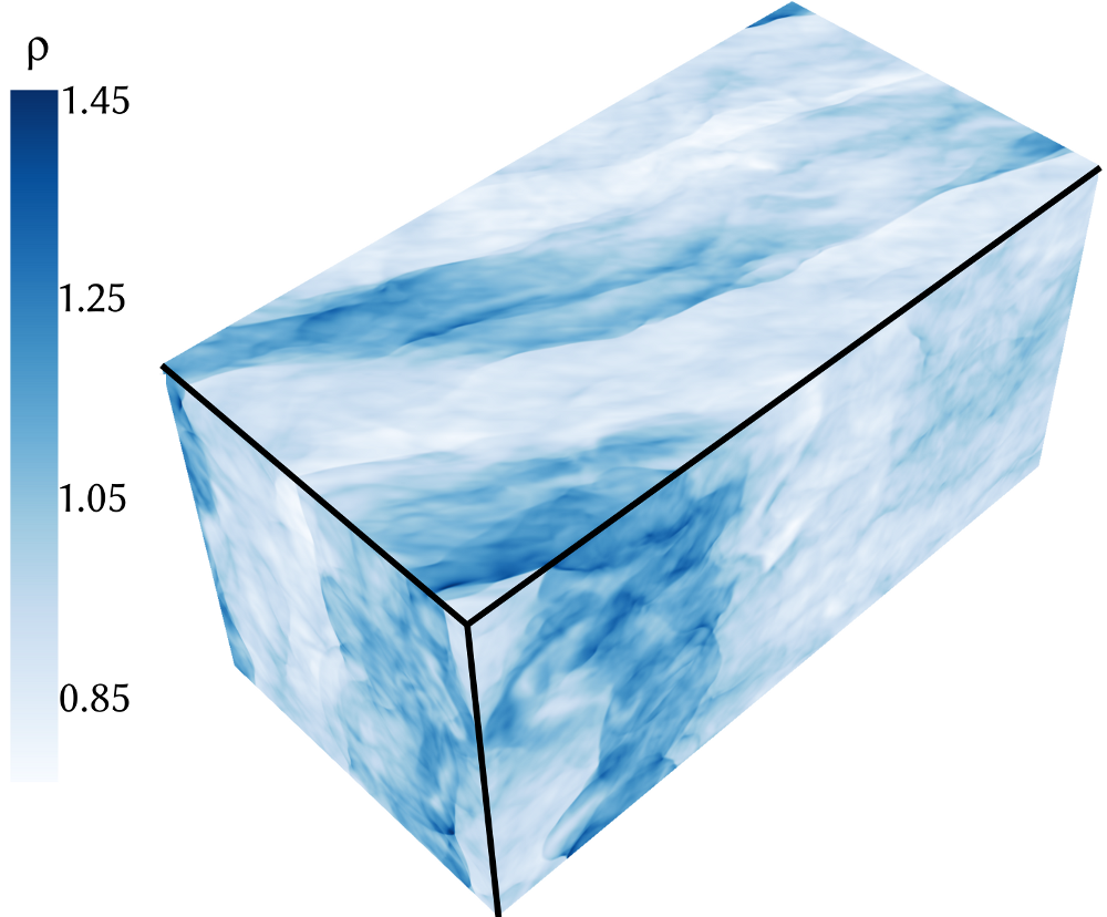
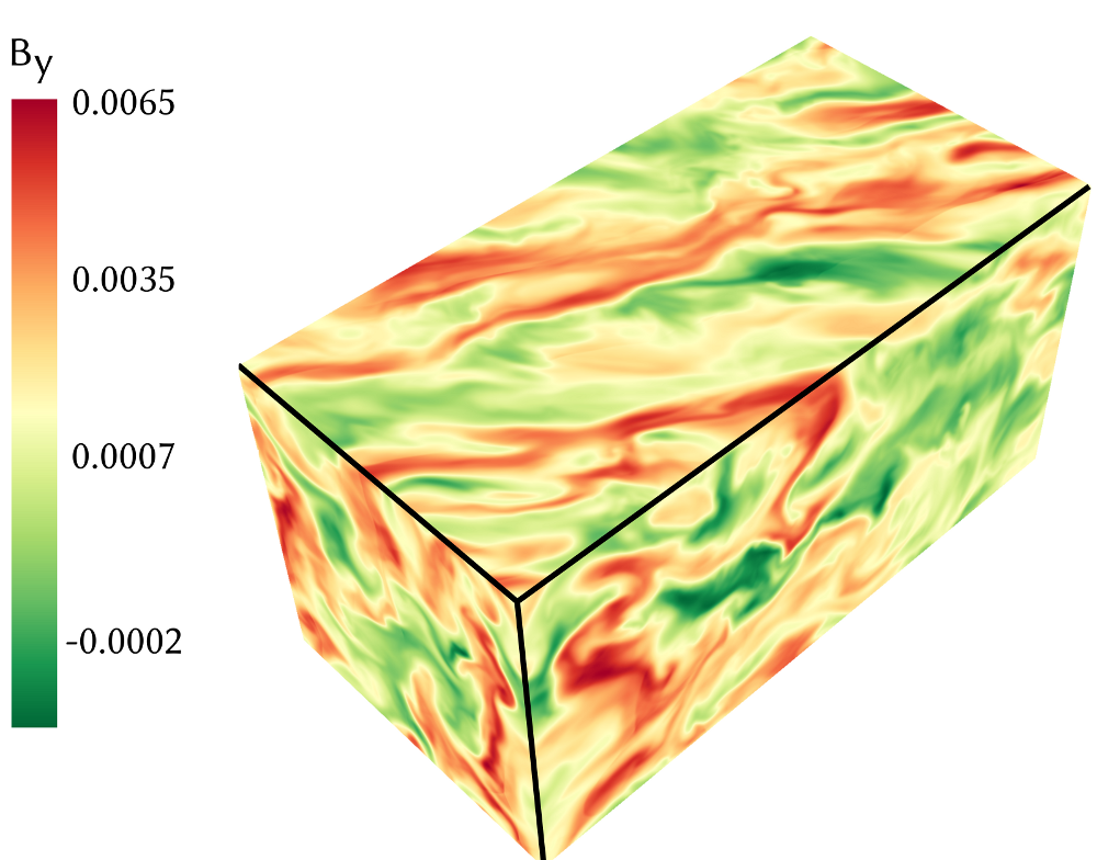
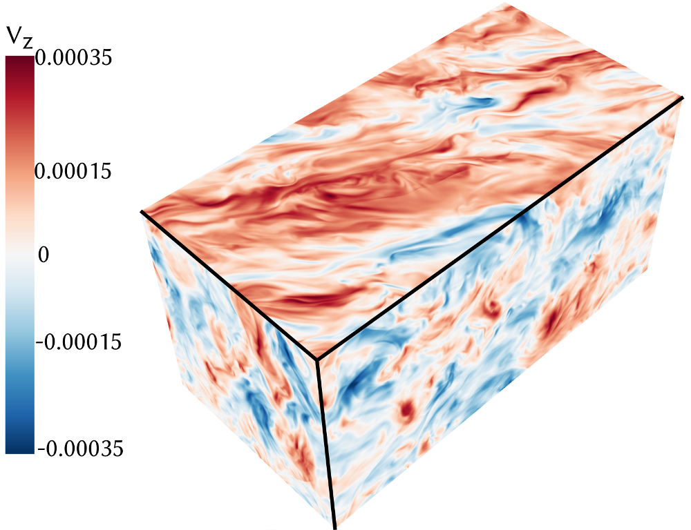
Figure 2: From left to right, 3D snapshots of $\rho$, $B_{y}$ and $v_{z}$ in model Y-C-Re85000 at the end of the simulation.

Because of the tremendous computational cost that was associated with that simulation, we start with a description of model Y-C-Re85000, performed with RAMSES. In this model, $Re=85000$ and $Pm=0.03$. This simulation was performed with a resolution $(N_{x},N_{y},N_{z})=(800,1600,800)$. Based on past experience and published results of simulations using the same setup at lower Reynolds number with a similar code (Simon & Hawley, 2009), we are confident that the small scales of the flow are properly accounted for in that simulation. In the $x$ and $z$ directions, the number of cells thus amounts to $800$ cells per disc scaleheight, which is the highest resolution ever achieved of MRI–driven MHD turbulence with a 2nd order compressible code. This gigantic simulation was run at the IDRIS supercomputing center on the BlueGen-Q machine Turing, using $32768$ cores. We found that the most efficient configuration was to use $4$ threads per cores, meaning that a total of $131\leavevmode\nobreak\ 072$ threads (or, equivalently, MPI sub–domains) were used. We used approximately $10$ hours of CPU time per timesteps. Running the simulation for over $35$ orbits ($\sim 10^{6}$ timesteps) thus required about $10^{7}$ hours of CPU time, corresponding to $300$ hours of wall clock time (i.e. about two weeks).

As described by Simon & Hawley (2009), in the presence of a mean azimuthal magnetic field, resistivity can prevent the linear instability from transiting to a turbulent state when the simulation starts from a laminar flow, even though it is found to remain turbulent on long timescales when that linear phase is bypassed. We thus adopted the method described by these authors and performed the run is two steps: we first solved the ideal MHD equations (i.e. with vanishing viscosity and resistivity parameters). The only dissipative effects are numerical in origin during that part of the calculation. A turbulent state is reached after $\sim 10$ orbits. The turbulent transport as measured by $\alpha$ displays fluctuations around a well defined mean value of about $6\times 10^{-2}$ for the next few orbits (see figure 1, top panel). At $t=15$, we restarted the simulation for an additional $20$ orbits with dissipation coefficients such that $Re=85000$ and $Pm=0.03$. As seen on the top panel of figure 1, the turbulence amplitude is quickly modified by the presence of those dissipation coefficients and reaches a new steady state after a few additional orbits. The nature of the flow is illustrated by a series of snapshots of the last time step of the run in figure 2. On the density plot one can recognize large scales density waves and low amplitude shocks. The turbulent magnetic field is dominated by large scale structures. On the contrary, the velocity snapshot shows both large and small scales structures, as expected given the very small $Pm$ used here.

We next averaged the transport rate after the system has reached a quasi steady state and until the end of the simulation. This period corresponds to $t>21$ orbits and is hatched on figure 1 (top panel). The value of $\alpha_{Rey}$, $\alpha_{Max}$ and $\alpha$ we obtained are $4.6\times 10^{-3}$, $1.3\times 10^{-2}$ and $1.8\times 10^{-2}$, respectively (see also Table 1). This $\alpha$ value is comparable to the one reported by Simon & Hawley (2009) for their most resolved run, for which $Pm=0.25$, $Rm=3200$ and $\beta=450$. The Maxwell and Reynolds stresses display a ratio of $\sim 3$ that is typical of such simulations. There is of course a degree of arbitrariness regarding the exact time at which we decide that the system has reached “a quasi steady state” and start averaging. We have checked that the statistics we consider do not vary significantly when making modest changes to the averaging period. For example, we find $\alpha=1.9\times 10^{-2}$ and $\alpha=1.8\times 10^{-2}$ when averaging over the periods $t>18$ and $t>25$ orbits, respectively. This is only a variation by $7\%$ and give an idea of the uncertainty associated with that measurement.

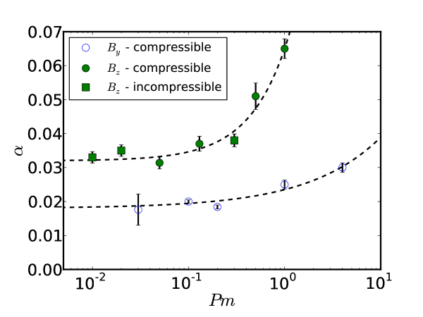
Figure 3: Mean value of the angular momentum transport (measured by means of $\alpha$) for the mean toroidal field simulations (blue circles), the mean vertical field simulations performed with RAMSES (green filled circles) and with SNOOPY (green filled squares). The dashed lines are power-law functions that approximately describe the data (see text).

To obtain a more accurate view of the energy budget at each scales, we also show on figure 1 (bottom panel) the time averaged power spectra. Because of the shearing box boundary conditions, we consider time dependent unsheared wave vector $\@vec{k}$ and the shell filter decomposition of the physical variables (Hawley et al., 1995). Being spherically symmetric, we note that this method filters out the information about the flow anisotropy which is known to be significant for MRI-driven turbulence (see Murphy & Pessah 2015, Figure 3. of Lesur & Longaretti 2011 and section 3.2.1). For each wavenumbers, the kinetic and magnetic energy are then given by

$$E_{K}(k) = \overline{v^{2}_{k}(k)/2}$$ (17)

$$E_{M}(k) = \overline{\@vec{B}^{2}_{k}(k)/2}\,,$$ (18)

respectively, where the bar denotes an average over time. Magnetic energy dominates at large scales ($k^{\prime}<15$, where we have defined $k^{\prime}=k/2\pi$ so that it corresponds to scales $l^{\prime}>H/15$) while kinetic energy dominates at smaller scales. This is a signature of the small $Pm$ value of the simulation, which implies that the resistive dissipation length is larger than the viscous dissipation length (Schekochihin et al., 2004). At small scales, the motions essentially correspond to hydrodynamic turbulence associated with a forward cascade (Lesur & Longaretti, 2011). We will exploit that scale separation in section 3.2 when designing sub-grid scale models for the hydrodynamic part of the flow. The kinetic energy power spectrum follows a power law with exponent $-3/2$ over the range $2<k^{\prime}<20$, thus covering one order in magnitude in spatial scales. The same exponent has been reported recently in other high resolution simulations of MRI–driven MHD turbulence both in the dynamo regime (Fromang, 2010) and in the presence of a net vertical field (Lesur & Longaretti, 2011), suggesting it is a general feature of the flow. We note that homogeneous forced MHD turbulence also displays the same exponent (Mason et al., 2008), although the result is still debated (Beresnyak, 2014). The surprising result here is that the magnetic energy does not show any obvious signature of a power–law regime, contrary to the case of homogeneous and driven MHD turbulence, while still being comparable in magnitude with $E_{K}$. More work is needed to clarify the reason for that discrepancy and to better understand the origin of the $-3/2$ exponent that is obtained in the case of MRI–driven MHD turbulence.

3.1.2 Angular momentum transport

We plot on figure 3 the total averaged stress $\alpha$ for all the resolved simulations we performed. Error bars $\sigma_{\alpha}$ are estimated with the method presented in Longaretti & Lesur (2010). In general, we find $\sigma_{\alpha}\sim 5\times 10^{-3}$ for the vertical field model (thus giving $\sigma_{\alpha}/\alpha\sim 5\%$). This is consistent with the estimate of Longaretti & Lesur (2010). The error estimate is smaller in the azimuthal field case, for which we obtained $\sigma_{\alpha}\sim 10^{-3}$ which corresponds to $\sigma_{\alpha}/\alpha\sim 1\%$. We note that we could not apply the same method for model ’Y-C-Re85000’ because of the short duration of the integration in that case. A simple standard deviation is thus plotted instead and explains the larger error bar for that particular model.

In agreement with previous results (see section 1) we find that $\alpha$ increases with Pm. However, the main result of figure 3 (and the main result of the paper) is that there is now convincing evidence of the convergence of the angular momentum transport rate at small $Pm$ toward a well defined, nonzero value. This is the case for both field geometry.

The azimuthal field case:

In this case, and with constant $Rm$ and $\beta$, we find that a fit to the data is given by the formula

$$\alpha_{By}=\alpha_{Bymin}+C_{y}Pm^{0.58}\,,$$ (19)

with the values of $\alpha_{Bymin}=1.8\times 10^{-2}$ and $C_{y}=5.5\times 10^{-3}$, respectively. This means that a good estimate of $\alpha$ is already obtained at $Pm=0.2$ for which a resolution of $128$ cells per unit length is sufficient. Indeed, we obtained $\alpha=1.8\times 10^{-2}$ which is equal to the asymptotic value of $\alpha$ at vanishingly low $Pm$.

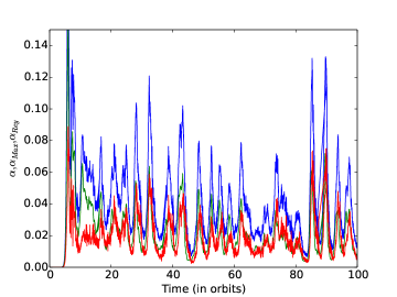
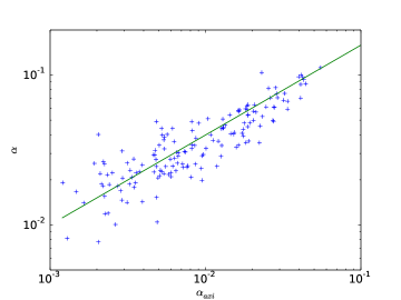
Figure 4: Left panel: Time history of $\alpha$ (blue curve), $\alpha_{Max}$ (red curve) and $\alpha_{Rey}$ (green curve) in model Z-C-Re3000. Right panel: scatter plot showing the total angular momentum transport rate $\alpha$ as a function of $\alpha_{axi}$ which measures the angular momentum transport due to $k_{y}^{\prime}=0$ and $k_{z}^{\prime}=1$ modes for $120$ dumps evenly spaced over model Z-C-Re3000. The green curve plots an approximate fit to the data (see text for details).

The vertical field case:

Here, we find a somewhat larger transport coefficient that can be fitted by the relation

$$\alpha_{Bz}=\alpha_{Bzmin}+C_{z}Pm^{1.1}$$ (20)

with $\alpha_{Bzmin}=3.2\times 10^{-2}$ and $C_{z}=3.3\times 10^{-2}$, with fixed $Rm$ and $\beta$. Moreover, there is good agreement between the compressible and incompressible approach in this vertical field case: for both flow type the simulations converge at small $Pm$ toward the same $\alpha$. As for the azimuthal field case, a good estimate of the asymptotic rate of angular momentum transport is already obtained for $Pm=0.13$ (using a resolution of $128$ cells per unit length), for which we found $\alpha=3.7\times 10^{-2}$, i.e. a value that differs by about $15\%$ from the asymptotic limit.

As already noted (section 2.4), in the presence of a vertical magnetic field we find that the time history of $\alpha$ displays significant variability. This is illustrated on figure 4 (left panel) for the particular case of model Z-C-Re3000 ($Pm=0.13$): while the time averaged transport rate amounts to $\alpha=3.7\times 10^{-2}$ in that case, there are numerous peaks during which it reaches values as high as $0.1$ that occur with a typical period of about $5$ to $10$ orbits. Such bursts are not unheard of in unstratified shearing boxes with a mean vertical field (Bodo et al., 2008; Latter et al., 2009) and have been attributed to recurrent ‘channel-like’ modes associated with the MRI. For the set of parameters we have considered here, the time history of $\alpha$ suggests that they contribute significantly to the turbulent transport. In an attempt to quantify that contribution, we have calculated for model Z-C-Re3000 the value $\alpha_{axi}$ of the transport that is due to axisymmetric ‘channel-like’ modes (for which $k_{y}^{\prime}=0$ and $k_{z}^{\prime}=1$) for $120$ dumps evenly spaced between $t=40$ and $t=100$. The mean value of $\alpha_{axi}$, averaged over all the dumps of the simulation, amounts to $1.2\times 10^{-2}$: this means that axisymmetric modes with $k_{z}^{\prime}=1$ accounts for $\sim 30\%$ of the angular momentum transport. In agreement with the results of Longaretti & Lesur (2010), angular momentum transport is dominated on average by non-axisymmetric modes even if the contribution of ‘channel-like’ modes is significant. The scatter plot showing the relation between $\alpha$ and $\alpha_{axi}$ for those $120$ dumps is shown on the right panel of figure 4, along with an indicative fit of the data given by

$$\alpha=\alpha_{0}\left(\frac{\alpha_{axi}}{\alpha_{axi0}}\right)^{0.6}\,,$$ (21)

with $\alpha_{0}=10^{-2}$ and $\alpha_{axi0}=10^{-3}$. The positive correlation between $\alpha$ and $\alpha_{axi}$ indicates that the relative contribution of the transport mediated by axisymmetric modes with $k_{z}^{\prime}=1$ increases during the bursts of activity: for example, $\alpha_{axi}$ amounts to only about $10\%$ of the transport when $\alpha=10^{-2}$ but, as indicated by Eq. (21), can contribute for up to $50\%$ of the turbulent activity when $\alpha=0.1$. These variations are consistent with the results of Latter et al. (2009) and with the idea that the bursts seen on figure 4 are due to large scale ‘channel-like’ modes (Bodo et al., 2008). We have repeated the same analysis for all the models and we have found a weak dependance of the relative fraction of axisymmetric transport with $Pm$: $\alpha_{axi}/\alpha=0.39$, $0.34$, $0.32$ and $0.29$, respectively for $Pm=1$, $0.5$, $0.13$ and $0.05$ and similar results for the incompressible runs with $\alpha_{axi}/\alpha=0.38$, $0.35$, respectively for $Pm=0.02$ and $0.01$,

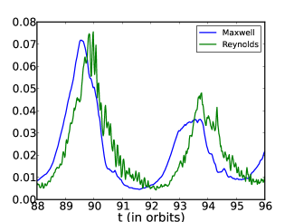
Figure 5: Time history of $\alpha_{Max}$ (blue curve) and $\alpha_{Rey}$ (green curve) in model Z-C-Re3000.

It is also noteworthy that the angular momentum transport in the presence of a vertical field is equally due to Maxwell and Reynolds stresses in the compressible simulation, whereas the classical ratio of approximately $3$ is obtained in an incompressible fluid or with an azimuthal field configuration for the specific values of $\beta$ and $Rm$ chosen in our investigation. The exact value of Maxwell to Reynolds stress ratio ($R$) are given in the last column of Tables 1,2, and 3. In an attempt to have a better understanding of the relative contribution of Maxwell and Reynolds stresses, we plot on figure 5 their time history over two burst cycles for the particular case of model Z-C-Re3000. This plot reveals that the Reynolds stress is larger than the Maxwell stress during the decaying part of the burst when the ‘channel-like’ modes (with $k_{y}=0$ and $k_{z}=1$) are destroyed by the non-linear turbulent dynamics. The computation of the contribution of the axisymmetric modes shows that the Maxwell transport is dominated by ‘channel-like’ modes whereas the Reynolds transport is due to non-axisymmetric modes. Because of the difference between the incompressible and compressible runs, we further speculate that such a destruction is associated with the excitation of compressible modes such as density waves. However this detailed study, not directly related to the angular momentum transport rate, is beyond the scope of this paper.

3.2 Large Eddy Simulations in the small Pm limit

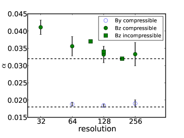
Figure 6: Mean value of the angular momentum transport (measured by means of $\alpha$) for the mean toroidal field LES simulation (implicit LES blue circles), the mean vertical field LES simulation performed with RAMSES (implicit LES, green filled circles) and with SNOOPY (Chollet-Lesieur LES, green filled squares). The resolution is given in number of cells per scaleheight. The dashed lines represents the asymptotic limits obtained with DNS.

The previous results have shown that angular momentum transport converges toward a well defined limit at small $P_{m}$. However, such simulations are very computationally expensive. Here, we investigate the possibility to use a sub-grid scale model instead of standard kinematic viscosity. The aim is to reduce the computational cost of the simulations without compromising the physics one may want to consider, such as the accretion rate or the turbulent power spectra.

Historically, the study of small $Pm$ flows has mostly relied on simulations using hyperviscosity such as geodynamo models (Glatzmaiers & Roberts, 1995) or small scale dynamo theory (Schekochihin et al., 2007). However, hyperviscosity is known to produce numerous artefacts in hydrodynamic turbulence, such as spectral bottlenecks, reduced intermittency and spurious isotropisation (Frisch et al., 2008). For this reason, we instead focus on Large Eddy Simulations (LES) in which the dissipation adapts dynamically to the turbulent cascade initiated by the large scales, thereby limiting the artefacts commonly due to hyperviscosity.

LES are routinely used in industrial applications to model flows at high $Re$. However, their MHD counterpart are not widespread, the reason being the higher complexity of the MHD turbulent cascade compared to the purely hydrodynamic cascade. Several subgrid-MHD models have been discussed in the literature including Smagorinsky (1963) type models (Yoshizawa, 1987) which can be used in finite difference/volume codes and Chollet & Lesieur (1981) type models (Baerenzung et al., 2008) targeted to spectral methods. However, most of these models are still under development and their applicability to $Pm\ll 1$ flows is yet to be proven.

In this work we have chosen to use well-known hydrodynamical subgrid models to treat the kinetic turbulent cascade only, leaving the induction equation with standard Ohmic resistivity. This approach is valid provided that the subgrid model is introduced at a scale much smaller than the resistive scale, so that the energy cascade is mostly hydrodynamical. Moreover, it has the advantage of using well-tested subgrid models which are reasonably simple to implement numerically. This type of methods has already been used to study Taylor-Green flows (Ponty et al., 2004) and dynamo action (Ponty et al., 2005) in the limit $Pm\rightarrow 0$. We therefore reproduce this approach using very similar tools in the MRI turbulence context.

3.2.1 Chollet-Lesieur model in incompressible simulations

Since our incompressible simulations are done with a spectral code, we have used the spectral subgrid model of Chollet & Lesieur (1981) (CL) to perform our incompressible LES. This model replaces the standard viscosity $\nu$ by the following expression in Fourier space:

$$\nu_{\mathrm{CL}}(k)=\Bigg{(}\frac{E(k_{c})}{k_{c}}\Bigg{)}^{1/2}\Big{(}0.267+9.21\exp[-3.03k_{c}/k]\Big{)}$$ (22)

where $k_{c}$ is the cutoff scale and $E(k_{c})$ is the kinetic energy at the cutoff scale . This expression encloses long range nonlinear interactions via a constant viscosity at $k\ll k_{c}$ and a cusp due to local energy transfers close to the cutoff scale $k_{c}$. Interestingly, $k_{c}$ is the only free parameter of this model. The amount of viscosity itself is automatically adjusted according to the amount of energy at the cutoff scale. It should be emphasized that this expression is only valid for 3D homogeneous and isotropic Kolmogorov turbulence. In principle, it is therefore not applicable to turbulent shear flows found in shearing box models since such flows are anisotropic (see section 3.1.1). As a first attempt to quantify that anisotropy, we proceed as follows. We define a decomposition in spherical harmonics such that

$$E_{K}(\bm{k})=\frac{1}{2}|\tilde{v}(\bm{k})|^{2}=\sum_{jm}c_{j}^{m}(|\bm{k}|)Y_{jm}(\hat{k}),$$ (23)

and similarly for the magnetic energy. We focus on the $l=2$ coefficients of that decomposition and define:

$$a_{2}=\sum_{m=-2}^{m=2}|c_{2}^{m}|^{2}/|c_{0}|^{2}.$$ (24)

$a_{2}$ takes significant values when there are strong variations of the energy over the shell, or, in other words, when the flow displays anisotropy at that scale. As shown in figure 7, it decreases with k but is still high at small scales for the kinetic energy. Nevertheless we will see that the Chollet-Lesieur model gives satisfactory results.

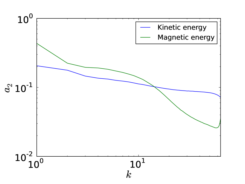
Figure 7: Estimate of the anisotropy at each scale. For each wavenumber, the energy is decomposed into spherical harmonics; the anisotropy is estimated from the sum of the second order coefficients normalized by the isotropic coefficient.

We have performed several simulations using CL subgrid model, varying $k_{c}$ and the resolution (runs Z-CL-XXX-X). Models labelled $a$ have $k_{c}/k_{\mathrm{max}}=0.75$ and models labelled $b$ have $k_{c}/k_{\mathrm{max}}=1$ where $k_{\mathrm{max}}$ is the maximum accessible wavenumber of the simulation (Table 3). As plotted on figure 6 (green squares), all of our models recover the statistical results of DNS with a reduced resolution. These encouraging results are confirmed by turbulent spectra compared to DNS simulation (figure 8). We find that both kinetic and magnetic spectra agree to less than 10% down to $k\sim 20$ with the highest resolution DNS Z-I-Re40000. We also find that simulations with $k/k_{c}=0.75$ exhibit the same convergence properties, at least for the resolution we studied. Therefore, the cutoff scale does not seem to have much impact on these results, provided it is below the resistive dissipation scale. These results demonstrate that CL models can be used efficiently to study low $Pm$ flows, with a gain in resolution of at least a factor 2 associated with a gain in computation time of at least a factor 20.

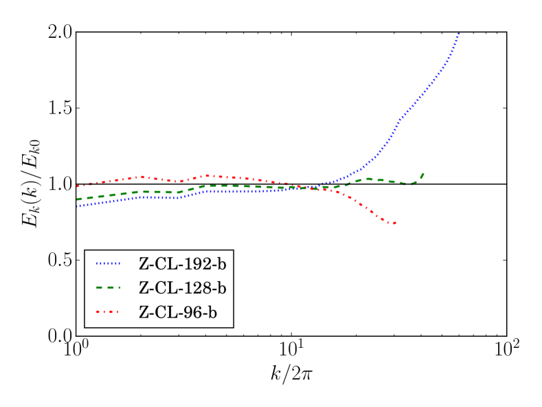
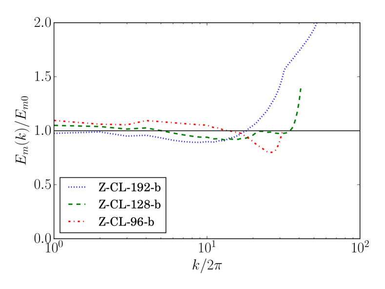
Figure 8: Ratio of power spectra of kinetic energy (top) and magnetic energy (bottom) obtained with a Chollet-Lesieur subgrid model with $k_{c}/k_{\mathrm{max}}=1$ and full DNS calculation at Re=40000.

3.2.2 Implicit LES in compressible simulations

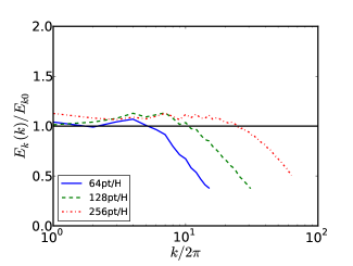
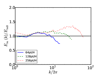
Figure 9: Ratio between the power spectra obtained with RAMSES in the ILES (green, red, blue and dotted curves) and model Y-C-Re85000 in the azimuthal magnetic field cases. Top panel is for kinetic energy power spectrum and bottom panel for magnetic energy power spectrum. On both panels, the black horizontal line mark the location of unity ratio.

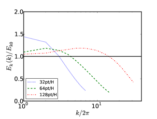
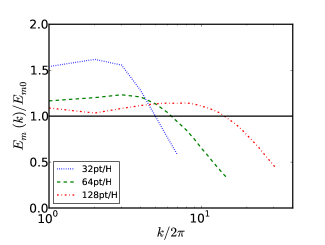
Figure 10: Same as figure 9, but for the vertical field case.

In the small $Pm$ limit, the simplest possible sub–grid scale model when using finite volume codes is certainly the so–called “Implicit LES” (ILES). The idea is to capture Ohmic resistivity explicitly in the simulation (since it occurs at large scale) but let numerical dissipation handle kinetic energy dissipation at small scales. This method has already been used in some previous works (Fleming et al., 2000; Inutsuka & Sano, 2005; Okuzumi & Hirose, 2011; Flock et al., 2012, 2015), but its range of validity has never been systematically and quantitatively investigated. In this section, we compare the results of such simulations, performed with RAMSES at various resolution with the results presented in section 3.1.

The azimuthal field case:

the magnetic Reynolds number is here fixed to $Rm=2600$ as for the DNS. We performed a series of simulations with resolutions ranging from $64$ to $256$ cells per scale height. For all cases, we obtain $\alpha=1.8\times 10^{-2}$, in very good agreement with our best resolved simulations at $Pm=0.03$ (see figure 6). We then compared the kinetic and magnetic energy power spectra in these simulations with the spectra obtained in the DNS with the lowest Prandlt number (Y-C-Re85000). In the upper panel (resp. lower panel) of figure 9, we plot the ratio of the kinetic (resp. magnetic) power spectra between the ILES and the DNS. The runs give an acceptable agreement with the DNS at all available scales (except at small scales in the kinetic energy, which is a result of the different hydrodynamical dissipation): at all resolutions, the deviations to the DNS run for $k^{\prime}<10$ for both the kinetic and the magnetic energy spectra, are at most of the order of $15\%$.

The vertical field case:

the resolution in this case was varied from $32$ cells per scale height to $256$ cells per scale height. As can be seen on figure 6, $\alpha$ decreases as resolution increases, most likely as a result of the decrease of the effective numerical viscosity, and converges to the value determined by the DNS simulations. Quite surprisingly though, the convergence as resolution is increased toward the asymptotic value of $\alpha$ at low $Pm$ is slower than the azimuthal field case, despite $Rm$ being much larger in that case. Indeed, with $64$ cells per scale height, the difference between the two $\alpha$ values is still of order $20\%$ while it has reached convergence in the case of a mean $B_{y}$. This is probably due to the stress dependence with $Pm$ being steeper in the presence of a mean vertical field. In any case, $128$ cells per scale height are needed to reach the asymptotic $\alpha$ value to less than $10\%$. We note that this is still a gain of a factor of $16$ in computing time. The power spectra displayed in figure 10 confirm that result: there is a difference of about $50\%$ between the power spectra of the ILES and the DNS at large scale for a resolution of $32$ cells per scale height. Even the largest resolution reveals differences of up to $20\%$ in both the kinetic and magnetic power spectra, even if the largest scales are converged to better than $10\%$, as expected from the good agreement between the transport coefficients in both simulations (figure 6).

4 Conclusions

We briefly summarise the main results and ideas of the paper and discuss some of their limitations.

Our main goal was to investigate the properties of the turbulent state in the small magnetic Prandtl number limit by mean of local DNS simulations. We showed that in the presence of a mean magnetic field threading the domain, angular momentum transport converges to a finite value in the small $Pm$ limit. This result is valid both with a vertical and with an azimuthal mean magnetic field with the asymptotic values at small $Pm$ being respectively: $\alpha=1.8\times 10^{-2}$ with $Rm=2600$ and $\beta_{y}\sim 10^{2}$ and $\alpha=3.2\times 10^{-2}$ with $Rm=400$ and $\beta_{z}=10^{3}$. The obtained values with our set of parameters are consistent with the estimations computed from the lifetime and accretion rate of protoplanetary discs ($\alpha$ is a few $10^{-2}$). Obviously, a word of care is in order here: the magnetization of accretion discs, such as protoplanetary discs, is only loosely constrained and the value of the $\beta$ parameter is unknown. $\alpha$ is known to strongly depend on the field strength, with $\alpha$ proportional to $\beta^{-1/2}$ (Hawley et al., 1995) or $\beta^{-1}$ (Bodo et al., 2011) in the vertical field case. Similarly, we can expect angular momentum transport to increase with the magnetic Reynolds number (Longaretti & Lesur, 2010). The asymptotic values of the angular momentum rate we obtained are thus only valid for the $\beta$ and $Rm$ parameters we considered, and with a scaling that remains to be determined in the small $Pm$ limit.

In the case of the compressible simulations with a mean vertical field, we obtained a surprising ratio of Maxwell to Reynolds stress of about $1$. Not withstanding any possible dependance with $\beta$ and $Rm$, we noticed that this ratio is related to the compressibility of the fluid, as a more usual value of about $3$ is obtained in the incompressible runs. It is also related to the bursty behavior of these two stresses: whereas a usual value is obtained in the growing phase of the bursts, the Reynolds stress dominates during its decreasing parts, resulting in a mean $R$ value of about $1$. This result is specific to the compressible simulations, but it implies that neither the Reynolds stress nor the Maxwell stress converge to the same value in compressible and incompressible simulations at low $Pm$. In fact, both stresses differ by about 50%, which we show can be attributed to their different behavior during the bursts. It is possible that the convergence of $\alpha$ at low $Pm$ to the same value with this two types of flow is fortuitous. In order to solve that issue, higher $Rm$ simulations are needed but are currently very costly.

Next, we investigated the interest of using large eddy simulations both in spectral and real spaces for such simulations. The simplest approach is to consider the implicit LES method. As expected, in all cases the smallest scales are not correctly handled, but it is possible to reproduce the large scales energy spectra by using a high enough resolution. To obtain an error smaller than $20\%$ on $\alpha$, the needed resolution corresponds to a fourth of the resolution needed when explicit viscosity is included. This corresponds to a decrease in CPU time by a factor $256$. To limit the computational cost of a simulation of a turbulent flow, explicit SGS models are also usually considered. The anisotropy of the rotating sheared flow and the turbulent cascade which differs from the Kolmogorov cascade, may indicate that simple SGS approaches are not well suited for MRI turbulence simulations. We tested the Chollet-Lesieur method which is used in spectral space and is applied directly on the spectrum components. This method is local in frequency space, the effective viscosity being a function of the wave-number, and there is a limited inclusion of the backscatter. We found that good results are also obtained with this Chollet-Lesieur approach notwithstanding the anisotropy of the flow at small scales.

Despite such positive results, a word of care is in order here. Although we showed that these methods are efficient to decrease the computational cost of MRI turbulence simulations, the needed resolution is still significant. For a magnetic Reynolds number $Rm=400$ with a vertical mean magnetic field, the required resolution is $64pts/H$. This $Rm$ is low compared to the values that are often chosen in the literature for which an even higher resolution is then necessary. To reach a turbulent flow dominated by Ohmic dissipation, a resolution of at least $256pts/H$ will be needed for $Rm$ values of a few thousands. Moreover, we considered only two diagnostics, namely the angular momentum transport rate and the power spectra, to reach this conclusion and other diagnostics, such as helicity or correlation functions, were not considered. Such statistical quantities may well be incorrectly described in our LES for the resolutions we used. More generally, with such reduced resolutions, any small scale process is not correctly handled, and for instance the study of collision of grains in protoplanetary discs or magnetic reconnection cannot be studied in such simulations.

Overall we still conclude that LES can be used to limit the computational time of future simulations. Future works should account for density stratification, which will be particularly relevant in the context of global simulations. Large scale phenomena such as the ones identified in the ‘butterflies diagrams’ can strongly modify the flow properties and are susceptible to affect the LES approach. Dedicated simulations should be performed to quantify the interest of such methods in this case.

References

- Baerenzung et al. (2008) Baerenzung, J., Politano, H., Ponty, Y., & Pouquet, A. 2008, Phys. Rev. E, 77, 046303
- Bai (2015) Bai, X.-N. 2015, ApJ, 798, 84
- Bai & Stone (2011) Bai, X.-N. & Stone, J. M. 2011, ApJ, 736, 144
- Bai & Stone (2013) Bai, X.-N. & Stone, J. M. 2013, ApJ, 769, 76
- Bai & Stone (2014) Bai, X.-N. & Stone, J. M. 2014, ApJ, 796, 31
- Balbus (2003) Balbus, S. A. 2003, ARA&A, 41, 555
- Balbus & Hawley (1991) Balbus, S. A. & Hawley, J. F. 1991, ApJ, 376, 214
- Balbus & Hawley (1998) Balbus, S. A. & Hawley, J. F. 1998, Reviews of Modern Physics, 70, 1
- Balbus & Henri (2008) Balbus, S. A. & Henri, P. 2008, ApJ, 674, 408
- Beresnyak (2014) Beresnyak, A. 2014, ApJ, 784, L20
- Biferale & Vergassola (2001) Biferale, L. & Vergassola, M. 2001, Physics of Fluids, 13, 2139
- Bodo et al. (2011) Bodo, G., Cattaneo, F., Ferrari, A., Mignone, A., & Rossi, P. 2011, ApJ, 739, 82
- Bodo et al. (2008) Bodo, G., Mignone, A., Cattaneo, F., Rossi, P., & Ferrari, A. 2008, A&A, 487, 1
- Brandenburg et al. (1995) Brandenburg, A., Nordlund, A., Stein, R. F., & Torkelsson, U. 1995, ApJ, 446, 741
- Chollet & Lesieur (1981) Chollet, J.-P. & Lesieur, M. 1981, Journal of Atmospheric Sciences, 38, 2747
- Evans & Hawley (1988) Evans, C. R. & Hawley, J. F. 1988, ApJ, 332, 659
- Fleming et al. (2000) Fleming, T. P., Stone, J. M., & Hawley, J. F. 2000, ApJ, 530, 464
- Flock et al. (2012) Flock, M., Henning, T., & Klahr, H. 2012, ApJ, 761, 95
- Flock et al. (2015) Flock, M., Ruge, J. P., Dzyurkevich, N., et al. 2015, A&A, 574, A68
- Frank et al. (2002) Frank, J., King, A., & Raine, D. J. 2002, Accretion Power in Astrophysics: Third Edition (Cambridge University Press)
- Frisch et al. (2008) Frisch, U., Kurien, S., Pandit, R., et al. 2008, Physical Review Letters, 101, 144501
- Fromang (2010) Fromang, S. 2010, A&A, 514, L5
- Fromang (2013) Fromang, S. 2013, in EAS Publications Series, Vol. 62, EAS Publications Series, 95–142
- Fromang et al. (2006) Fromang, S., Hennebelle, P., & Teyssier, R. 2006, A&A, 457, 371
- Fromang et al. (2007) Fromang, S., Papaloizou, J., Lesur, G., & Heinemann, T. 2007, A&A, 476, 1123
- Glatzmaiers & Roberts (1995) Glatzmaiers, G. A. & Roberts, P. H. 1995, Nature, 377, 203
- Guan et al. (2009) Guan, X., Gammie, C. F., Simon, J. B., & Johnson, B. M. 2009, ApJ, 694, 1010
- Hawley & Balbus (1992) Hawley, J. F. & Balbus, S. A. 1992, ApJ, 400, 595
- Hawley et al. (1995) Hawley, J. F., Gammie, C. F., & Balbus, S. A. 1995, ApJ, 440, 742
- Hawley et al. (1996) Hawley, J. F., Gammie, C. F., & Balbus, S. A. 1996, ApJ, 464, 690
- Herault et al. (2011) Herault, J., Rincon, F., Cossu, C., et al. 2011, Phys. Rev. E, 84, 036321
- Inutsuka & Sano (2005) Inutsuka, S.-i. & Sano, T. 2005, ApJ, 628, L155
- Johansen et al. (2009) Johansen, A., Youdin, A., & Klahr, H. 2009, ApJ, 697, 1269
- King et al. (2007) King, A. R., Pringle, J. E., & Livio, M. 2007, MNRAS, 376, 1740
- Kunz & Lesur (2013) Kunz, M. W. & Lesur, G. 2013, MNRAS, 434, 2295
- Latter et al. (2009) Latter, H. N., Lesaffre, P., & Balbus, S. A. 2009, MNRAS, 394, 715
- Lesur et al. (2014) Lesur, G., Kunz, M. W., & Fromang, S. 2014, A&A, 566, A56
- Lesur & Longaretti (2007) Lesur, G. & Longaretti, P.-Y. 2007, MNRAS, 378, 1471
- Lesur & Longaretti (2011) Lesur, G. & Longaretti, P.-Y. 2011, A&A, 528, A17
- Longaretti & Lesur (2010) Longaretti, P.-Y. & Lesur, G. 2010, A&A, 516, A51
- Mason et al. (2008) Mason, J., Cattaneo, F., & Boldyrev, S. 2008, Phys. Rev. E, 77, 036403
- Masset (2000) Masset, F. 2000, A&AS, 141, 165
- Miyoshi & Kusano (2005) Miyoshi, T. & Kusano, K. 2005, Journal of Computational Physics, 208, 315
- Murphy & Pessah (2015) Murphy, G. C. & Pessah, M. E. 2015, ApJ, 802, 139
- Okuzumi & Hirose (2011) Okuzumi, S. & Hirose, S. 2011, ApJ, 742, 65
- Ponty et al. (2005) Ponty, Y., Mininni, P. D., Montgomery, D. C., et al. 2005, Physical Review Letters, 94, 164502
- Ponty et al. (2004) Ponty, Y., Politano, H., & Pinton, J.-F. 2004, Physical Review Letters, 92, 144503
- Riols et al. (2013) Riols, A., Rincon, F., Cossu, C., et al. 2013, Journal of Fluid Mechanics, 731, 1
- Riols et al. (2015) Riols, A., Rincon, F., Cossu, C., et al. 2015, A&A, 575, A14
- Sagaut (2006) Sagaut, P. 2006, Large Eddy Simulation for Incompressible Flows (Springer)
- Schekochihin et al. (2004) Schekochihin, A. A., Cowley, S. C., Taylor, S. F., Maron, J. L., & McWilliams, J. C. 2004, ApJ, 612, 276
- Schekochihin et al. (2007) Schekochihin, A. A., Iskakov, A. B., Cowley, S. C., et al. 2007, New Journal of Physics, 9, 300
- Shakura & Sunyaev (1973) Shakura, N. I. & Sunyaev, R. A. 1973, A&A, 24, 337
- Simon et al. (2013) Simon, J. B., Bai, X.-N., Armitage, P. J., Stone, J. M., & Beckwith, K. 2013, ApJ, 775, 73
- Simon & Hawley (2009) Simon, J. B. & Hawley, J. F. 2009, ApJ, 707, 833
- Simon et al. (2011) Simon, J. B., Hawley, J. F., & Beckwith, K. 2011, ApJ, 730, 94
- Smagorinsky (1963) Smagorinsky, J. 1963, Monthly Weather Review, 91, 99
- Stone & Gardiner (2010) Stone, J. M. & Gardiner, T. A. 2010, ApJS, 189, 142
- Stone et al. (1996) Stone, J. M., Hawley, J. F., Gammie, C. F., & Balbus, S. A. 1996, ApJ, 463, 656
- Teyssier (2002) Teyssier, R. 2002, A&A, 385, 337
- Yoshizawa (1987) Yoshizawa, A. 1987, Physics of Fluids, 30, 1089