From localized spot to the formation of invaginated labyrinth structures in spatially extended systems

Abstract

The stability of a circular localized spot with respect to azimuthal perturbations is studied in in a variational Swift-Hohenberg model equation. The conditions under which the circular shape undergoes an elliptical deformation that transform it into a rod shape structure are analyzed. As it elongates the rod-like structure exhibits a transversal instability that generates an invaginated labyrinth structure which invades all the space available.

I Introduction

Many spatially extended systems that undergo a symmetry breaking instability close to a second-order critical point can be described by a real order parameter equation in the form of a Swift-Hohenberg type model, which has been derived in various field of nonlinear science such as hydrodynamics SH77 , chemistry Hilali , plant ecology efeverPlant , and nonlinear optics Tlidi93 .

A complex Swift-Hohenberg equation was deduced in the context of lasers Paul ; Lega1 ; Lega2 and optical parametric oscillators Longhi . Moreover, to describe the nascent optical bistability with transversal effect in nonlinear optical cavities a real approximation has been deduced TML from laser equations. This approximation allowed to predict stable localized structures and organized clusters of them TML . A detailed derivation of this equation from first principles can be found in Ref. Paul . In this work, we show that this real modified Swift-Hohenberg equation (SHE) of the form

$$\partial_{t}u=\eta+\epsilon u-u^{3}-\nu\nabla^{2}u-\nabla^{4}u$$ (1)

supports a curvature instability on localized structures that leads to an elliptical deformation that produces a rod-like structure. As the time evolution is further increases, the rod-like structure exhibits a transverse undulation and leads to the formation of invaginated structures. This structure is a labyrinthine pattern diefined by an interconnected structure where the field value is high. The outer part or complement to the invaginated structure corresponds to low field value. This behavior occurs far from any pattern forming instability and requires a bistable behavior between homogeneous steady states. In Eq. (1), $u=u(x,y,t)$ is a real scalar field, $x$ and $y$ are spatial coordinates and $t$ is time. The parameter $\eta$ represents the external forcing field which brakes the reflection symmetry $u\rightarrow-u$. The bistability parameter is $\epsilon$. The coefficient $\nu$ in front of a diffusive term $\nabla^{2}$ may change the sign and allows the pattern forming to take place Tlidi93 ; CrossHohenberg ; hohen ; pismenTB ; VLM11 . Depending on the context in which this equation is derived, the physical meaning of the field variable and parameters adopt different meanings, for instance, in cavity nonlinear optics $u(x,y,t)$ corresponds to light field intensity, while parameters $\{\eta,\epsilon,\nu\}$ are associated with the injection field, the deviations of the cavity field, and cooperativity, respectively TML .

For certain range of parameter values, Eq. (1) exhibits stable circular localized structures, for $\eta<0$ localized structures appear as isolated peaks of the field $u(x,y,t)$, instead, for $\eta>0$ localized structures are holes in the field. These localized structures have a fixed stable radius for each parameter value. Curvature instability of localized spot has been experimentally studied or theoretically predicted in magnetic fluids Dickstein93 , in liquid crystals Oswald1990 ; Oswald2000 , in reaction-difusion systems Pearson ; LEE ; Pismen-2002 ; Munuzuri ; Kaminaga1 ; Kaminaga2 ; Kolok ; Davis ; Muraotv ; Schaak98 ; Pismen-2002 ; Hayase1 ; Hayase2 , in plant ecology Meron , in material science Ren ; Nishiura , in granular fluid systems and in frictional fluids Sandnes1 ; Sandnes2 , and nonlinear optics TVP02 . The fingering instability of planar fronts leading to the formation of labyrinth structures has been reported by Hagberg et al. Hagberg . In this manuscript we shall focus on circular localized states.

II Stability of localized spot

Considering fixed parameter values, starting with an azimuthally symmetric localized structure. The structure is perturbed, this perturbation grows radially as shown in Fig. 2.1. The circular shape becomes unstable at some critical radius. The elliptical shape elongate into a rod like structures as shown in Fig. 1. This elongation proceeds until a critical size is reached beyond which a transversal instability onset the appearance of fingers near the mid section of the structure (see Fig. 2.3). The finger continues to elongate, and the amplitude of oscillation increases (Figs. 2.4 and 2.5). The dynamic of the system does not saturate and for a long time evolution, the rod-like structure invades the whole space available in ($x$, $y$)-plane as shown in Fig. 2.6. This invaginated structure is stationary solutions of the SHE. The dynamic described previously has been observed in cholesteric liquid crystals under the presence of an external electric field Oswald1990 ; Oswald2000 , where an initially circular structure of cholesteric phase suffers from curvature instability, transversal oscillations and develops into an extended labyrinthine structure. The characterization of this dynamic is an open problem.

For $\nu=2$, the bifurcation diagram of the model Eq. (1) in the parameter space ($\epsilon$, $\eta$) is shown in Fig. 3. For $\epsilon>0$ the system undergoes a bistable regime between homogeneous steady states. For $\epsilon<0$, the system has only one homogeneous steady state. The curve $\Gamma_{1}$ represent the coordinates of the limit points of the bistable curve ($\eta_{\pm}=\pm 2(\epsilon/3)^{3/2}$). The threshold associated with a symmetry breaking instability is provided by the curve $\Gamma_{2}$. The coordinates of the symmetry breaking instabilities thresholds are $\eta_{\pm}=\pm\sqrt{(\nu^{2}+4\epsilon)/3}(\nu^{2}-8\epsilon)/24$. Curve $\Gamma_{3}$, built numerically separates the zone where localized structures are stable, $II$-zone, from the zone where they are unstable, $I$-zone. The transition from localized structures to labyrinthine pattern occurs when crossing from $I$-zone to $II$-zone through the $\Gamma_{3}$-curves indicated in Fig. 3. This transition occurs via fingering instability at the $\Gamma_{3}$-curves delimiting the parameter domain $I$ and $II$. In the limit of the classical Swift-Hohenberg equation, $\eta=0$, there is no observation of fingering instability, instead the transition from II to I zones, localized structures only grow radially. As a result of boundary conditions destabilization of this structures into labyrinthine structures is observed, this is a size effect phenomenon. Contrary, for $\eta\neq 0$ the transition from II to I zones of a localized spot is affected from curvature instability, giving rise to an unstable rod structure which exhibits transversal oscillations and develops into an extended labyrinthine structure.

In what follows, we first study analytically the stability of a circular localized spot with respect to azimuthal perturbation. This mode analysis allows us to evaluate the threshold above which the transition from localized spot to a rod-like structure takes place. Then, we perform the linear stability analyzis of the rod-like structure and determine the conditions under which the transversal oscillations occur for the SH equation.

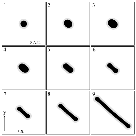
Figure 1: Temporal evolution for; 1) $t=0$; 2) $t=125$; 3) $t=175$; 4) $t=225$; 5) $t=275$; 6) $t=340$; 7) $350$; 8) $360$; 9) $t=400$, of a localized spot into an elliptical deformation and then to a rod-like structure for Eq. (1) with parameters: $\eta=-0.065$; $\epsilon=2.45$; $\nu=2.0$. Minima are plain white. The image corresponds to a zoom of $16\times 16$ points of a $512\times 512$ point finite-difference simulation.

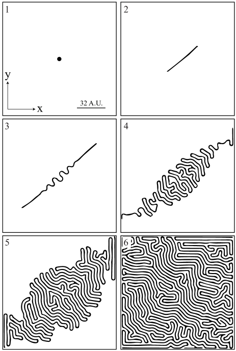
Figure 2: Transition from a single localized spot to invaginated pattern. Temporal evolution with Neumann boundary conditions and with the same parameters as in Fig. 1. 1) $t=0$, Localized spot, 2) $t=600$, rod-like structure, 3) $t=1900$, transverse undulation of the rod-like structure 4) $t=2800$, and 5) $t=3700$, localized transient patterns, and 6) $t>15000$, stationary invaginated labyrinth pattern. Minima are plain white and the mesh integration is $512\times 512$. Simulation done with finite-difference method

.

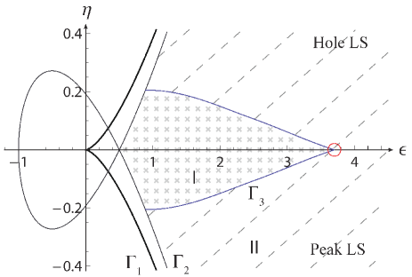
Figure 3: (Color online) Bifurcation diagram of Eq. (1) in ($\epsilon$, $\eta$) space for $\nu=2.0$. In $II$-zone (dashed black), stable circular localized structures are observed. In $I$-zone (grey crosses) generation of labyrinthine structures are observed from localized structures.

Starting from a solution with rotational symmetry (i.e circular localized structure) $u=u_{s}(r-r_{s})$ where $r$ is the radial coordinate and $r_{s}$ characterizes the localized structure radius. Then we perturb the solution $u(X,t)=u_{s}(X)+W(r,r_{s},r_{0})$ with $X$ is the relative position $X\equiv(r-(r_{s}+r_{0}(\theta,t)))$, where $r_{0}$ is the perturbed radius position, which accounts for the interface of the localized structure, $\theta$ stands for the angular coordinate, and $W\ll 1$ are corrections to the circular localized spot. Using polar representation of Eq. (1), considering the above perturbation and parameters in Eq. (1) at linear order in $W$ one obtains

$$\mathcal{L}W=\partial_{t}r_{0}\partial_{X}u_{s}+\eta+\epsilon u_{s}-u_{s}^{3}-\nu\nabla^{2}u_{s}-\nabla^{4}u_{s},$$ (2)

where the lineal operator $\mathcal{L}\equiv-(\epsilon+3u_{s}^{2}-\nu\nabla^{2}-\nabla^{4}).$ which is a self-adjoint. Assuming that the radius of the localized structure is sufficiently large, the operator $\mathcal{L}$ which is explicitly dependent on the radial coordinate can be approximated by a homogeneous operator in this radial coordinate

$$\mathcal{L}\approx-\epsilon-3u_{s}^{2}+\nu\left(\partial_{r}^{2}+\frac{1}{r_{s}}\partial_{r}\right)+\left(\partial_{r}^{4}+\frac{2}{r_{s}}\partial_{r}^{3}\right),$$ (3)

this operator possesses a neutral mode, i.e., zero eigenvalue with the eigenfuction $\partial_{X}u_{s}$. This approach allows us to perform analytical calculations, which are not accessible when the operator is inhomogeneous. Using this approach the solvability condition (see textbook pismenTB and references therein) yields

$$\partial_{t}r_{0}=-\Delta\frac{1}{r_{s}^{2}}\partial_{\theta}^{2}r_{0}+\frac{6\beta}{r^{4}_{s}}\partial_{\theta}^{2}r_{0}(\partial_{\theta}r_{0})^{2}-\frac{1}{r^{4}_{s}}\partial_{\theta}^{4}r_{0}+\frac{2\beta}{r^{3}_{s}}(\partial_{\theta}r_{0})^{2},$$ (4)

where

$$\beta\equiv\frac{\langle\partial_{XX}u_{s}|\partial_{XX}u_{s}\rangle}{\langle\partial_{X}u_{s}|\partial_{X}u_{s}\rangle},$$ (5)

and

$$\Delta\approx\left(\nu-2\beta\right).$$ (6)

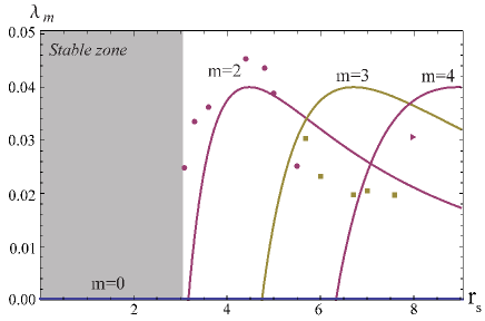
Figure 4: (Color online) Lines show approximated theoretical growth rate as function of the localized structure radius for $m=0,2,3$ using formula (7). Points show numerical results for growth rates of modes: $m=2$ (circles), $m=3$ (squares), and $m=4$ (triangle). With parameters: $\eta=-0.065$; $\epsilon=2.45$; $\nu=2$; $dx=0.5$; $dt=0.03$. The insets show the different perturbation modes of a localized structure.

Then the field $r_{0}(\theta,t)$ satisfies a nonlinear diffusion equation. The first, the second, the third and the last term on the right side of Eq. (4) account for the linear diffusion, the non-linear diffusion, the hyper-diffusion and nonlinear advection, respectively. When $\Delta<0$ the localized structure is stable, and for $\Delta>0$, the localized state is unstable as result of the curvature instability. For a better understanding of Eq. (4) one can study the stability of different perturbation modes as follows.

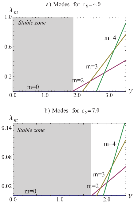
Figure 5: (Color online) Theoretical growth rate as function of $\nu$ using formula (7), for parameters: $\eta=-0.065$; $\epsilon=2.45$. Emergence of instability modes for fixed radii, for 1) $r_{s}=4.0$, and 2) $r_{s}=7.0$.

To study the stability of 2D localized structures, we perturb $r_{0}$ with fluctuations of the form $r_{0}(\theta,t)=R_{0}Re\text{[}\exp(im\theta+\lambda_{m}t)\text{]}$, where, $m$ is integer number, $\theta\in\text{[}0,2\pi\text{[}$, $R_{0}$ an arbitrary small constant, and $Re$ denotes the real part. By substituting this perturbations in Eq. (4) and linearizing in $R_{0}$, we get the growth rate relation

$$\lambda_{m}(r_{s})=(\nu-2\beta)\left(\frac{m}{r_{s}}\right)^{2}-\left(\frac{m}{r_{s}}\right)^{4}.$$ (7)

Even though the previous analysis has been made considering a fixed value for the radius of the localized structure, this radius is determined by balance between the interface energy and the energy difference between the homogeneous states. The interface energy and energy difference are proportional to $\nu$ and $\eta$ parameter, respectively. The radius of the localized structures $r_{s}$ is proportional to $\nu/\eta$ coulletLS , however no analytical expression is available. Hence, the possible radius only lower bounded. This lower bound is determined by the size of the core of the front between homogeneous states. For the sake simplicity, to figure out the role of the growth rate relation we consider that $r_{s}$ is an independent parameter. Then, for studying the effect of the curvature on the modal instability, one can consider an artificial circular structure of any given radius $r_{s}$ and evaluate its stability. Figure 4 shows the growth rate $\lambda_{m}$ as a function of the radius of circular 2D localized structures for different values of angular index $m$. For fixed values of all parameters, the stability of the localized structure is affected with its radius. For small radius, the mode $m=0$ causes radial growth without any change on the structures shape. Only modes $m\neq 0$ affect the circular shape of the localized structures. The angular mode $m=2$ becomes unstable ($\lambda_{2}>0$) and leads to an elliptical deformation of the circular shape of the localized structure as shown in Fig 2.2. This mode has a larger domain of instability and an elliptical deformation occurs for $r_{0}=5.7$ as shown in Fig. 4. Triangular deformation corresponding to the angular index $m=3$ occurs for $r_{0}=7.9$. It has been shown that for fixed parameter values, different modes emerge by means of the localized structure’s radius increment. Nevertheless, if the radius of the localized structure is fixed, one expects that by the variation of a control parameter, lets say $\nu$, one could control the emergence of certain unstable modes (cf. Fig. 5). In the above results, we have considered that the radius of the localized structure is large, however, this approximation is not always valid. Numerical simulations compared to approximate analytical results of the growth rate of localized structures is shown in Fig. 4, numerically, an unstable circular spot of arbitrary radius is generated by hand. From this graphs we conclude that the approximate analysis of the $\mathcal{L}$ operator considering $r_{s}$ as an independent parameter gives a qualitative description of the observed dynamics. Moreover, the approximated growth rates coincide in magnitude to numerical observations, and the transition radius between unstable modes are consistent. On the other hand, the stability analysis of $\mathcal{L}$ is only accessible numerically.

Let us fix the value of the radius to $r_{s}=4.0$ and to $r_{s}=7.0$, and let now the diffusion coefficient $\nu$ be the control parameter. For these values, the first angular index $m$ mode to become unstable is $m=2$ as shown in Fig. 5. From this figure we see that when increasing $\nu$, higher order modes become unstable. Comparison between the two different values of the radius shows the higher unstable modes appear at lower range of values for $\nu$ when increasing the radius $r_{0}$.

III Transversal instability of rod structures and emergence of labyrinthine patterns

The SHE Eq. (1) admits a single stripe like solution TLM98 ; k41 . In order to evaluate the threshold over which transversal oscillations appear, we perform the stability analysis of a rod-like structure, by a method similar to the one performed in Ref. Hagberg . For this purpose we perturb the single stripe solution as $u=u_{f}(\boldsymbol{\xi})+W(\boldsymbol{x},\boldsymbol{X_{0}})$ where $u_{f}$ is the single stripe solution and $\boldsymbol{\xi}=\boldsymbol{x}-\boldsymbol{X_{0}}(y,t)$ the relative position, $\boldsymbol{X_{0}}$ is the field that accounts for the shape and evolution of the finger, and $W(\boldsymbol{x},\boldsymbol{X_{0}})<<1$ is a non-linear correction of a single stripe. Applying this ansatz in Eq. (1) at first order in $W$ and applying the solvability condition pismenTB , the following equation is obtained for the dynamic of $\boldsymbol{X_{0}}$

$$\partial_{t}X_{0}=-\Delta^{\prime}\partial_{yy}X_{0}+6\beta^{\prime}\partial_{y}^{2}X_{0}(\partial_{y}X_{0})^{2}-\partial_{y}^{4}X_{0},$$ (8)

where

$$\beta^{\prime}=\frac{\langle\partial_{\xi\xi}u_{f}|\partial_{\xi\xi}u_{f}\rangle}{\langle\partial_{\xi}u_{f}|\partial_{\xi}u_{f}\rangle},\text{ and }\Delta^{\prime}=(\nu-2\beta^{\prime}).$$ (9)

Thus $\boldsymbol{X_{0}}$ satisfies a nonlinear diffusion equation. This equation describes the dynamics of an interface between two symmetric states Chevallard ; Calisto . This model is well known for exhibiting a zigzag instability. Analogously, to the previous section, when $\Delta<0$ the single stripe solution is stable, and for $\Delta>0$, the solution is unstable as result of the curvature instability. From equation (8) one expects to observe the single stripe becomes unstable by the appearance of an undulation. Figure 6 shows the emergence of this undulated rod-like structure. Note that similar dynamical behavior is observed in the propagation of cholesteric finger in liquid crystals Oswald1990 ; Oswald2000 . Later, this undulated stripe is replaced by the emergence of facets that form a zigzag structure. However the higher nonlinear terms control the evolution of the single stripe, then the dynamics of initial zigzag is replaced by the growth of undulations without saturation as it is depicted in Fig. 2.4. Therefore, the system displays the emergence of a roll-like pattern which is formed in the middle section of the structure and invades the system generating invaginated structure. (see Fig. 2.5).

Figure 6: (Color online) Transversal instability of a single infinite stripe of Eq. (1). Image shows a section of a 256$\times$256 point simulation with periodic boundary conditions using a pseudo-spectral code. Parameters: $\eta=-0.065$, $\epsilon=2.45$, $\nu=2$, $dx=0.5$, and $dt=0.03$.

IV Conclusions

In this paper we have described the stability of localized spot in a Swift-Hohenberg equation. We first constructed a bifurcation diagram showing different solutions that appear in different regimes of parameters. Then we have shown that the angular index $m=2$ becomes first unstable as consequence of curvature instability. This instability leads to an elliptical deformation of the localized spot. Other type of deformations corresponding to $m=3$, $4$ and $5$ occur also in a Swift-Hohenberg equation. We have shown also that for a fixed values of the localized spot radius, the angular index $m=2$ becomes unstable for small diffusion coefficient while higher order modes $m>2$ become unstable for large values of a diffusion coefficient.

When angular index $m=2$ becomes unstable, the curvature instability of localized spot produces an elliptical deformation leading to the formation of rod-like structure. Subsequently, it generates undulations in the rod-like structure. In the course of time, the space time dynamics leads to the formation of invaginated labyrinth structures. To understand this dynamics, we have performed the stability of a single stripe localized structure.

It should be noted that by an offset transformation, $u\rightarrow u+u_{0}$, where $u_{0}$ is a constant, Eq. (1) can be rewritten in such a way that the constant parameter $\eta$ is removed and a quadratic nonlinearity appears. This quadriatic model is equivalent to Eq. (1). The model with a quadratic nonlinearity has been well studied (see the textbook pismenTB and the references therein). This equivalence implies that the results of the present work are also valid for physical systems described by the quadratic model.

- (1) J. Swift and P. C. Hohenberg, Phys. Rev. A 15, 319 (1977).
- (2) M’F. Hilali, G. Dewel, and P. Borckmans, Phys. Lett. A 217, 263 (1996).
- (3) R. Lefever et al., J. Theor. Biol. 261, 194 (2009).
- (4) M. Tlidi, M. Georgiou, and P. Mandel, Phys. Rev. A 48, 4605 (1993).
- (5) P. Mandel, Theoretical Problems in Cavity Nonlinear Optics, Cambridge University Press,(1997).
- (6) J. Lega, J.V. Moloney, and A.C. Newell, PRL 73, 2978 (1994).
- (7) J. Lega,J.V. Moloney, and A.C. Newell, Physica D 83(4), 478-498 (1995).
- (8) S. Longhi, and A. Geraci, Phys. Rev. A 54, 4581 (1996).
- (9) M. Tlidi, P. Mandel, and R. Lefever PRL 73(5), 640 (1994).
- (10) M.C. Cross, and P.C. Hohenberg Rev. Mod Phys. 65, 851 (1993).
- (11) P.C. Hohenberg, and B.I. Halperin, Rev. Mod. Phys. 49, 435 (1977).
- (12) L. M. Pismen Patterns and Interfaces in Dissipative Dynamics, (Springer Series in Synergetics, Berlin Heidelberg 2006).
- (13) A.G. Vladimirov, R. Lefever, and M. Tlidi, Phys. Rev. A 84, 043848 (2011).
- (14) A. J. Dickstein, S. Erramilli, R. E. Goldstein, D. P. Jackson, S. A. Langer, Science 261, 1012 (1993).
- (15) P. Ribiere and P. Oswald, J. De Physique 51, 1703 (1990).
- (16) P. Oswald, J. Baudry, and S. Pirkl, Phys. Rep. 337, 67 (2000).
- (17) J. E. Pearson, Science 261 , 189 (1993).
- (18) K. Lee, W. D. McCormick, J. E. Pearson, and H. L.Swinney, Nature (London) 369, 215 (1994).
- (19) A. P. Munuzuri, V. Perez-Villar, and M. Markus, Phys. Rev. Lett. 79, 1941 (1997).
- (20) A. Kaminaga, V. K. Vanag, and I. R. Epstein, Angew. Chem. 45, 3087 (2006).
- (21) A. Kaminaga, V. K. Vanag, and I. R. Epstein, J. Chem. Phys. 122, 174706 (2005).
- (22) T. Kolokolnikov and M. Tlidi, Phys. Rev. Lett. 98, 188303 (2007).
- (23) P. W. Davis, P. Blanchedeau, E. Dulos, and P. De Kepper, J. Phys. Chem. A 102, 8236 (1998).
- (24) C.B Muratov and V. V. Osipov, Phys. Rev. E 53 , 3101 (1996); 54, 4860 (1996); C.B Muratov, Phys. Rev. E 66, 066108 (2002).
- (25) M. Monine, L. Pismen, M. Bar and M. Or-Guil, J. Chem. Phys. 117, 4473 (2002).
- (26) A. Schaak and R. Imbihl, Chemical Physics Letters, 283, 368 (1998).
- (27) Y. Hayase and T. Ohta, Phys. Rev. Lett. 81, 1726 (1998).
- (28) Y. Hayase and T. Ohta , Phys. Rev. E 62 , 5998 (2000).
- (29) E. Meron, E. Gilad, J. von Hardenberg, and M. Shachak, Chaos Solitons Fractals 19, 367 (2004).
- (30) X. Ren and J. Wei, SIAM J. Math. Anal. 35, 1 (2003).
- (31) Y. Nishiura and H. Suzuki, SIAM J. Math. Anal. 36, 916 (2004).
- (32) B. Sandnes, H. A. Knudsen, K. J. Maloy, and E. G. Flekkoy, Phys. Rev. Lett. 99, 038001 (2007).
- (33) B. Sandnes, E.G. Flekkoy, H.A. Knudsen, K.J. Maloy, and H. See, Nature Communications, 2, 288 (2011).
- (34) M. Tlidi, A. G. Vladimirov, and P. Mandel, Phys. Rev. Lett. 89, 233901 (2002).
- (35) A. Hagberg, A. Yochelis, H. Yizhaq, C. Elphick, L. Pismen, E. Meron, Physica D 217, 186 (2006).
- (36) P. Coullet, Int. J. of Bif. and Chaos 12-11, 2445-2457 (2002).
- (37) M. Tlidi, P. Mandel, and R. Lefever, Phys. Rev. Lett. 81, 979 (1998).
- (38) M. Tlidi, P. Mandel, M. LeBerre, E. Ressayre, A. Tallet and L. Di Menza, Opt. Lett. 25, 487 (2000).
- (39) C. Chevallard, M. Clerc, P. Coullet and J.-M. Gilli, Europhys. Lett. 58, 686 (2002).
- (40) H. Calisto, M. Clerc, R. Rojas, E. Tirapegui, Phys. Rev. Lett. 85, 3805 (2000).