Competition of magneto-dipole, anisotropy and exchange interactions in composite multiferroics

Abstract

We study the competition of magneto-dipole, anisotropy and exchange interactions in composite three dimensional multiferroics. Using Monte Carlo simulations we show that magneto-dipole interaction does not suppress the ferromagnetic state caused by the interaction of the ferroelectric matrix and magnetic subsystem. However, the presence of magneto-dipole interaction influences the order-disorder transition: depending on the strength of magneto-dipole interaction the transition from the ferromagnetic to the superparamagnetic state is accompanied either by creation of vortices or domains of opposite magnetization. We show that the temperature hysteresis loop occurs due to non-monotonic behavior of exchange interaction versus temperature. The origin of this hysteresis is related to the presence of stable magnetic domains which are robust against thermal fluctuations.

I Introduction

Multiferroic materials are materials with coupled magnetic and electric degrees of freedom. Cheong and Mostovoy (2007); Khomskii (2006); Katsura et al. (2005); Mostovoy (2006); Kimura (2007) One example of this coupling is due to spin-orbit interaction in certain crystals. However, this coupling is relatively weak. Currently there is an active search for multiferroic materials with strong coupling. Ederer and Spaldin (2005); Kornev et al. (2007)

One way to strongly coupled magnetic and electric degrees of freedom is to develop hybrid ferroelectric-ferromagnetic layered materials where mechanical stress produces strong correlations between the layers. Fiebig (2005); Eerenstein et al. (2006); Ramesh and Spaldin (2007); Sone et al. (2012) Recently another promising possibility has been suggested based on granular materials where small metallic ferromagnetic (FM) grains were embedded into ferroelectric (FE) matrix or these grains were located in close proximity to the FE substrate. Udalov et al. (2014) The presence of small metallic grains increases the strength of Coulomb interaction providing the necessary coupling between the FE and FM degrees of freedom.

An important question is to understand the nature of multiferroic state in granular multiferroic materials. On the mean-field level the properties of these materials have been understood. Udalov et al. (2014) It was shown that the exchange coupling $J$ depends on the properties of the FE matrix/substrate, in particular on the dielectric permittivity $\epsilon$ of the surrounding medium. Udalov et al. (2014, 2015) Due to temperature dependence of dielectric permittivity, $\epsilon(T)$, the exchange interaction depends non-monotonically on temperature leading to the inverse phase transition with paramagnetic phase appearing at lower temperatures compared to the ferromagnetic phase. The qualitative behavior of $J$ is different for small and large (compared to the grain size $r_{\rm gr}$) inter-grain distances $a$: for large inter-grain distances, $a>r_{\rm gr}$, the $J$-value is increased in the vicinity of the FE Curie point due to suppression of the Coulomb blockade effects leading to a different magnetic state at these temperatures.

However, it is still an open question whether the magneto-electric coupling obtained in the mean-field theory is robust against the magneto-dipole and anisotropy interactions neglected in the mean-field approach. We use the numerical modelling to address this question.

We investigate the non-equilibrium meta-stable states in granular system and study the nature of new meta-stable phases appearing in the system with temperature dependent exchange interaction. In addition, we answer the question if temperature dependent exchange interaction can lead to unusual blocking effects.

To be more specific, we study the magnetic behavior of composite multiferroics with $\operatorname{\mathit{T}_{\mathrm{\scriptscriptstyle C}}^{\mathrm{\scriptscriptstyle FE}}}<\operatorname{\mathit{T}_{\mathrm{\scriptscriptstyle C}}^{\mathrm{\scriptscriptstyle FM}}}$, where $\operatorname{\mathit{T}_{\mathrm{\scriptscriptstyle C}}^{\mathrm{\scriptscriptstyle FE}}}$ is the FE Curie temperature of paraelectric-ferroelectric transition of the FE matrix and $\operatorname{\mathit{T}_{\mathrm{\scriptscriptstyle C}}^{\mathrm{\scriptscriptstyle FM}}}$ is the Curie temperature of FM grains. We focus on the temperature range $T\ll\operatorname{\mathit{T}_{\mathrm{\scriptscriptstyle C}}^{\mathrm{\scriptscriptstyle FM}}}$ where all grains are in the FM state and study the phase diagram of granular multiferroics beyond the mean-field approximation using Monte-Carlo simulations. In particular, we study the combined effect of magnetic anisotropy, the long-range magneto-dipole (MD) interaction and the exchange coupling. We show that there is an inverse magnetic transition in the system which is robust with respect to the MD interaction. This inverse transition disappears only for strong MD interaction, stronger than the exchange coupling. In addition, we show that non-monotonic temperature behavior of intergrain exchange interaction leads to a new type of hysteresis in composite multiferroics.

Three-dimensional (3D) nanostructures composed of single-domain ferromagnetic particles has been intensively studied both experimentally and theoretically. Woi nska et al. (2013); Liua and Bertram (2001); Gong et al. (1991); Laurent et al. (1989); Liou and Chien (1988); Bedanta and Kleemann (2009); Chantrell et al. (2000); Kechrakos and Trohidou (1998a); Petracic et al. (2004) The interplay of magnetic anisotropy, long-range magneto-dipole interaction and short range exchange interaction defines the magnetic state of the system. Depending on the ratio of these interactions different magnetic states are possible in granular ferromagnets. Kleemann et al. (2001); Petracic et al. (2006) Among them are superparamagnetic (SPM), super spin-glass (SSG) and superferromagnetic (SFM) states.

The most studied situation is related to the case of large intergrain distances ($\geq 2$nm) and small exchange interaction where magnetic state is defined by the competition of MD interaction and anisotropy. Sankar et al. (2000); Kechrakos and Trohidou (1998a); El-Hilo et al. (1998) The magnetic anisotropy is responsible for “blocking” phenomena and defines the blocking temperature $T_{\mathrm{b}}$. Liou and Chien (1988); Chien (1988) The weak MD interaction modifies the blocking temperature, while the strong MD interaction leads to the SSG state. Ayton et al. (1995); Ravichandran and Bagchi (1996); Mamiya et al. (1999); Djurberg et al. (1997); Sahoo et al. (2003)

For small distances between grains ($\sim 1$ nm) the exchange interaction is crucial. It leads to the formation of the SFM state. Timopheev et al. (2012); Kleemann et al. (2001); Scheinfein et al. (1996); Kondratyev and Lutz (1998); Bedanta et al. (2007) In such systems the SPM-SFM transition occurs. Even a weak exchange interaction can influence the magnetic state of the system. Scheinfein et al. (1996) In particular, the FM ordering with long range ferromagnetic correlations appears.

Different theoretical methods have been used to study granular magnets. The mean-field approach allows to study granular systems with finite short range exchange interaction and zero (or weak) MD interaction neglecting fluctuation effects. Atherton and Beattie (1990); Timopheev et al. (2009) Modelling based on Landau-Lifshitz equation allows to consider the MD, magnetic anisotropy and exchange interactions. Wiedwald et al. (2004) However, this approach needs to be generalized in the presence of thermal fluctuations by introducing the Langevin forces. Garcia-Palacios and Lazaro (1998) These fluctuations are important for granular magnetic systems since the granular magnetic moment is relatively small and fluctuation effects are pronounced especially near the phase transitions. However, the inclusion of Langevin forces in the nonlinear spin dynamics is not numerically efficient. Therefore we use Monte-Carlo (MC) simulations which allow to study phase transitions in composite multiferroics with strong long-range MD interaction and arbitrary thermal fluctuations. Serena et al. (1993a); ElHilo et al. (1994); Kechrakos and Trohidou (1998a); El-Hilo et al. (1998); Petracic et al. (2006); Liua and Bertram (2001); Asselin et al. (2010); Atxitia et al. (2010); Du et al. (2010); Woi nska et al. (2013)

MC modelling strongly depends on the degree of anisotropy. At strong anisotropy the problem reduces to the Ising model with magnetic moment of each particle having only two directions defined by the anisotropy axis. In this case the MC modelling is very efficient and is based on the trial spin flips. Another type of MC modelling is based on the Heisenberg model with arbitrary magnetization direction. This model is more general but it requires more computational time due to spin rotations over the sphere rather than spin flips. Matsubara and Itoya (1993); Hinzke and Nowak (1999); Asselin et al. (2010); Atxitia et al. (2010) We use our own MC code with random spin-flips and random spin-rotations that is valid for any anisotropy.

The paper is organized as follows: In Sec. II we formulate our main results. In Sec. III we discuss the model of composite multiferroics. In Sec. IV we introduce important physical quantities which we calculate. We discuss our results in Sec. V. The details of our numerical calculations are presented in Appendix A.

II Main results

Here we summarize our main results. The non-monotonic temperature dependence of exchange interaction in composite multiferroics leads to the unusual evolution of the magnetic state with temperature. The intergrain exchange interaction has either peak or deep in the vicinity of the FE phase transition due to coupling of electric and magnetic degrees of freedom.  In the mean field approximation the peak in the exchange interaction leads to the onset of FM state in the vicinity of FE phase transition. The deep in the exchange interaction suppresses the FM state in the vicinity of the FE Curie point. We use Monte-Carlo simulations to investigate the influence of long-range MD interaction and magnetic anisotropy on the magnetic phase diagram of composite multiferroics. We show that MD interaction and anisotropy do not suppress the magneto-electric coupling in these materials, however their interplay produces a new type of hysteresis. Our results are the following:

1) The Monte-Carlo simulations reproduce the mean field results in the absence of MD interaction and magnetic anisotropy. Similar to the mean field approach, the FM state exists in the vicinity of the FE Curie point and the disordered state appears away from this region.

2) The finite MD interaction does not suppress the FM ordering in the vicinity of the FE phase transition even if the MD interaction is twice stronger than the exchange interaction. The presence of MD interaction leads to the appearance of the domain structure and to splitting of uniform FM state. This result is similar to Ref. Scheinfein et al., 1996, where a weak FM interaction leads to the formation of FM domains, while strong MD interaction produces a vortex structure.

3) The magnetic state depends on the strength of MD interaction outside the FM region: the system is in the SPM state for weak MD interaction and in the antiferromagnetic stripe phase for strong MD interaction.

4) The magnetic anisotropy does not influence the FM state. However, it prevents the formation of vortices in the transition region and leads to a widening of the FM domain.

5) The “blocking phenomenon” does not appear at finite magnetic anisotropy and zero MD interaction at considered temperatures meaning that the system has enough time to reach the ground state such that the non-equilibrium state does not appear.

6) The “blocking phenomenon” appears at finite magnetic anisotropy and finite MD interaction. The temperature hysteresis loop occurs due to non-monotonic behavior of exchange interaction vs. temperature. The origin of this hysteresis is related to the presence of stable magnetic domains which are robust against thermal fluctuations, MD, exchange, and anisotropy interactions.

7) The AFM stripes appear in the case of deep in the exchange interaction.

Below we discuss these results in details.

III The model

III.1 Magnetic subsystem

In this subsection we consider the magnetic subsystem. We model a composite multiferroic as an ensemble of FM grains embedded into FE matrix. All grains are homogeneously magnetized single domain FM particles of the same volume $V$ and saturation magnetization $M_{s}$. For temperatures $T\ll\operatorname{\mathit{T}_{\mathrm{\scriptscriptstyle C}}^{\mathrm{\scriptscriptstyle FM}}}$, the saturation magnetization $M_{s}$ is constant. Each grain with volume $V$ has a magnetic moment $\mu=M_{s}V$ and is treated as a point dipole located at the centre of the grain. The grains are pinned to the sites of the regular cubic lattice with lattice spacing $a$ and can freely rotate their adjusting magnetic moments.

The whole system is modelled as a $3D$ lattice of classical spins, with magnetic moment of the $i$th grain being ${\bm{\mu}}_{i}=\mu{\bf S}_{i}$, where the unit vector ${\bf S}_{i}=(S_{i}^{x},S_{i}^{y},S_{i}^{z})$ is the spin of $i$th particle representing the direction of the magnetic moment.

We assume that each grain has a uniaxial anisotropy. Spatial distributions of anisotropy axes varies in different experiments and depends on the preparation condition. The anisotropy axes can be homogeneously distributed over the solid angle, or uniformly distributed in a certain plane. We assume that the easy axes of all grains are oriented in the z-direction. This situation is realized in experiment with magnetic field applied during the sample preparation. Bedanta et al. (2007)

The Hamiltonian of the system has the form

$${\cal H}={\cal H}_{\rm exc}+{\cal H}_{\rm dip}+{\cal H}_{\rm an}.$$ (1)

The first term, ${\cal H}_{\rm exc}$, describes the exchange coupling between grains $i$ and $j$

$${\cal H}_{\rm exc}=-J\sum\limits_{\langle i,j\rangle}{\bf S}_{i}\cdot{\bf S}_{j},$$ (2)

where the sum is over the nearest neighbour pairs of grains.

The second term, ${\cal H}_{\rm dip}$, in Eq. (1) describes the long-range magneto-dipole (MD) interaction between magnetic moments ${\bm{\mu}}_{i}$ and ${\bm{\mu}}_{j}$ of individual grains

$${\cal H}_{\rm dip}=g\sum\limits_{i<j}{\,}\frac{{\bf S}_{i}\cdot{\bf S}_{j}{\,}r^{2}_{ij}-3({\bf S}_{i}\cdot{\bf r}_{ij})({\bf S}_{j}\cdot{\bf r}_{ij})}{r^{5}_{ij}},$$ (3)

where ${\bf r}_{ij}$ is the distance between magnetic moments at sites $i$ and $j$ measured in units of lattice spacing $a$ and $g$ is the MD interaction constant.

The third term, ${\cal H}_{\rm an}$, in Eq. (1) describes uniaxial anisotropy energy

$${\cal H}_{\rm an}=-K\sum_{i}({\bf e}_{z}\cdot{\bf S}_{i})^{2},$$ (4)

where $K$ is the temperature independent magnetic anisotropy energy of a single grain. The unit vector ${\bf e}_{z}$ defines the direction of the anisotropy easy axis.

We consider the energy parameters $(J,g,K,T)$ in arbitrary units. Parameters, $g$ and $K$ depend on a grain volume and can be controlled by varying the grain size. The dipole coupling $g$ is additionally depends on the lattice spacing $a$. This allows one to vary parameters $g$ and $K$ in a wide range. The exchange interaction is proportional to the grain surface and scales with the volume as $V^{2/3}$. Moreover, the ratio of MD and exchange interactions can be controlled by varying the interparticle distance $a$. The MD interaction decays as $1/a^{3}$ with distance, while exchange interaction decays exponentially $e^{-\kappa a}$, where $\kappa$ is the inverse length which depend on the band structure of the surrounding FE matrix and the Fermi energy of electrons inside grains.

III.2 Ferroelectric subsystem

The FE matrix is characterized by the Curie temperature $\operatorname{\mathit{T}_{\mathrm{\scriptscriptstyle C}}^{\mathrm{\scriptscriptstyle FE}}}$. We study the temperature region in the vicinity of $\operatorname{\mathit{T}_{\mathrm{\scriptscriptstyle C}}^{\mathrm{\scriptscriptstyle FE}}}$. The most important characteristic of the FE matrix in our consideration is the FE dielectric permittivity $\epsilon$ which has a peculiarity in the vicinity of the phase transition point, $\operatorname{\mathit{T}_{\mathrm{\scriptscriptstyle C}}^{\mathrm{\scriptscriptstyle FE}}}$. Strukov and Levanyuk (1998) This peculiar behavior of $\epsilon$ provides a strong coupling between electric and magnetic degrees of freedom. Udalov et al. (2014, 2015)

III.3 Interaction of magnetic and ferroelectric subsystems

Recently the intergrain exchange interaction, $J$, in composite multiferroics was studied and its temperature behavior was predicted. Udalov et al. (2014, 2015) In the vicinity of the FE phase transition the exchange interaction has a peculiarity. Depending on the system parameters it has either peak or deep. Such peculiarity appears due to combine influence of Coulomb blockade effects and the temperature dependence of dielectric permittivity of the FE matrix on the exchange interaction. The peculiarity of the exchange interaction in the vicinity of the FE Curie point $T=\operatorname{\mathit{T}_{\mathrm{\scriptscriptstyle C}}^{\mathrm{\scriptscriptstyle FE}}}$ is related to the peculiarity in the dielectric permittivity $\epsilon$ of the FE matrix. The exchange interaction as a function of $\epsilon$ has the form Udalov et al. (2014)

$$J(T)=J_{0}\epsilon^{\gamma a/r_{\rm gr}-1},$$ (5)

where parameter $J_{0}>0$ is the $\epsilon$-independent part of exchange interaction, $J_{0}$ decays exponentially with intergrain distance $a$; $\gamma$ is the numerical coefficient of order one. The dielectric permittivity $\epsilon$ has a peak at temperature $T=\operatorname{\mathit{T}_{\mathrm{\scriptscriptstyle C}}^{\mathrm{\scriptscriptstyle FE}}}$. For $\gamma<r_{\rm gr}/a$ (small intergrain distances) the exchange interaction has a deep, while for $\gamma>r_{\rm gr}/a$ (large intergrain distances) it has a peak.

The dependence of the intergrain exchange interaction $J$ on the FE permittivity $\epsilon$ is the signature of magneto-electric coupling emerging in composite multiferroics. The peak of exchange interaction leads to the unusual magnetic phase diagram: the FM state appears in the vicinity of the FE Curie temperature $\operatorname{\mathit{T}_{\mathrm{\scriptscriptstyle C}}^{\mathrm{\scriptscriptstyle FE}}}$, while away from $\operatorname{\mathit{T}_{\mathrm{\scriptscriptstyle C}}^{\mathrm{\scriptscriptstyle FE}}}$ the system is in the SPM state. Thus, the FM state in the system exists in a finite region around FE Curie point, $\operatorname{\mathit{T}_{\mathrm{\scriptscriptstyle C}}^{\mathrm{\scriptscriptstyle FE}}}$. In case of deep in the temperature dependence of exchange constant $J$ the opposite situation occurs: the FM state is suppressed in the vicinity of $\operatorname{\mathit{T}_{\mathrm{\scriptscriptstyle C}}^{\mathrm{\scriptscriptstyle FE}}}$ due to interaction of magnetic and FE subsystems.

Above effects have been studied in Ref. Udalov et al., 2014 using the mean field approximation without taking into account the MD interaction and anisotropy. Here we take into account both interactions and study the influence of MD interaction and magnetic anisotropy on the magneto-electric coupling in composite multiferroics.

For large inter-grain distances, $\gamma>r_{\rm gr}/a$, the exchange interaction $J(T)$ has the peak. In this work we model this peak as follows

$$J(T)=J_{0}e^{-(T-\operatorname{\mathit{T}_{\mathrm{\scriptscriptstyle C}}^{\mathrm{\scriptscriptstyle FE}}})^{2}/w^{2}},$$ (6)

where $w$ is the width of the exchange peak and $J_{0}$ is the amplitude of intergrain exchange interaction. The peak in $J(T)$ occurs at temperatures $T=\operatorname{\mathit{T}_{\mathrm{\scriptscriptstyle C}}^{\mathrm{\scriptscriptstyle FE}}}$, when the Coulomb blockade is suppressed and the electron wave functions become weakly localized leading to a strong overlap and strong exchange interaction. Udalov et al. (2014) The Coulomb blockade is suppressed when permittivity $\epsilon(T)$ reaches its maximum value at $T=\operatorname{\mathit{T}_{\mathrm{\scriptscriptstyle C}}^{\mathrm{\scriptscriptstyle FE}}}$.

For small inter-grain distances, $\gamma<r_{\rm gr}/a$, the exchange interaction $J(T)$ has a deep which we model as follows

$$J(T)=J_{0}\left(1-e^{-(T-\operatorname{\mathit{T}_{\mathrm{\scriptscriptstyle C}}^{\mathrm{\scriptscriptstyle FE}}})^{2}/w^{2}}\right).$$ (7)

IV Calculated quantities

In this section we introduce physical quantities which we calculate. The calculation procedure is described in Appendix A. The first quantity we calculate is the average magnetization Lau and Dasgupta (1989); Holm and Janke (1993); Peczak et al. (1991); Chen et al. (1993)

$$M(T)=\left|\frac{1}{N}\sum\limits_{i=1}^{N}{\bf S}_{i}\right|,$$ (8)

where $N$ is the number of lattice sites.

In the presence of MD interaction and zero external magnetic field, the average magnetization $M(T)$ is not an efficient quantity: the lattice spins form complex magnetic patterns, either domains or vortices, and the mean magnetization vanishes, $1/N\sum_{i}{\bf S}_{i}=0$, even if locally the system is in the FM state. To account for local FM correlations we introduce the cell averaged magnetization, $m(T)$, over a cell with linear size $L_{c}$. We find that the optimal size for such cell average is $L_{c}=5$

$$m(T)=\left\langle\left|\frac{1}{N_{c}}\sum\limits_{i}{\bf S}_{i}\right|\right\rangle,$$ (9)

where summation is over the all grains in a given cell $N_{c}=L_{c}^{3}$ and the averaging is defined as summation over the all possible positions of the cell centre, $\langle\rangle=N^{-1}\sum_{i}$.

Next, we introduce the spin-spin correlation function $G$ as an averaged correlation function for nearest-neighbour pairs

$$G=\frac{1}{N}\sum\limits_{\bf R}\frac{1}{6}\sum\limits_{\bf g}\langle{\bf S}_{\bf R}\cdot{\bf S}_{\bf R+g}\rangle=\frac{1}{3N}\sum\limits_{\langle i,j\rangle}\langle{\bf S}_{i}\cdot{\bf S}_{j}\rangle,$$ (10)

where ${\bf g}$ are the six vectors of nearest neighbours and the last summation ${\langle i,j\rangle}$ is over the all nearest-neighbour pairs in the lattice. The correlation function $G$ is important for understanding magneto-transport in granular magnets. The magneto-resistance (MR) of granular magnetic film is proportional to this correlation function, MR(T)$\sim G$. The MR measurements can be considered as the probes of the magnetic state of the system.

V Discussion of results

V.1 Influence of magneto-dipole (MD) interaction on the magnetic phase diagram of composite multiferroics

In this subsection we discuss the influence of MD interaction on the magnetic phase diagram of composite multiferroics for the case of large inter-grain distances, where exchange interaction $J$ has a peak around $\operatorname{\mathit{T}_{\mathrm{\scriptscriptstyle C}}^{\mathrm{\scriptscriptstyle FE}}}$, see Eq. (6).

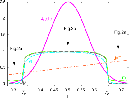
Figure 1: (Color online) Magnetic phase diagram of composite multiferroic vs. temperature for zero magneto-dipole interaction ($g=0$) and magnetic anisotropy ($K=0$). Solid (red) line shows the temperature dependence of intergrain exchange interaction, $J(T)$. Straight dash dotted (orange) line stands for temperature $T$. Gray dash dot-dotted and green dotted lines show the average magnetization $M(T)$ and cell averaged magnetization $m(T)$, respectively. Blue dashed line shows the nearest neighbour correlation function $G$. Transition temperatures $T_{\mathrm{\scriptscriptstyle C}}^{\pm}$ are defined using the mean-field equation, $T=2J(T)$.

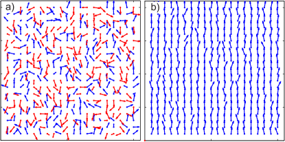
Figure 2: (Color online) Snapshots of single magnetic layer of composite multiferroic. Panels (a) and (b) show the disordered (SPM) magnetic state and the ordered FM state, respectively. Position of these panels is shown in Fig. 1 by black arrows.

V.1.1 Zero magneto-dipole (MD) interaction

In the absence of long-range MD interaction and anisotropy the magnetic phase diagram obtained using the Monte-Carlo simulations coincides with the mean-field phase diagram (see Fig. 1). We used the following parameters: $J_{0}=2.5$, $\operatorname{\Delta\mathit{T}^{\mathrm{\scriptscriptstyle FE}}}=0.1$, $\operatorname{\mathit{T}_{\mathrm{\scriptscriptstyle C}}^{\mathrm{\scriptscriptstyle FE}}}=0.5$. These parameters correspond to Fe grains embedded into organic TTF-CA FE matrix. The grain size is $5-10$ nm and the intergrain distance $\geq 1$ nm. For these parameters the intergrain exchange interaction is about $J\sim 300$K. The Curie temperature of bulk ferroelectric TTF-CA is $80$ K. However, for granular array it can be smaller; the Curie temperature of TTF-CA in composite granular metal/FE system is $50$ K. Huth et al. (2014)

The FM state appears around $\operatorname{\mathit{T}_{\mathrm{\scriptscriptstyle C}}^{\mathrm{\scriptscriptstyle FE}}}$, where $J(T)$ has a maximum (see snapshot in Fig. 2b) and the SPM state exists outside this region (see Fig. 2a). The finite FM region appears with two magnetic phase transitions due to peak in the exchange interaction. In the mean-field approximation both transition temperatures $T_{\mathrm{\scriptscriptstyle C}}^{\pm}$ are defined as $T=2J(T)$. Due to zero MD interaction domains are not formed, the ground state of the system is the homogeneous FM state and the magnetization $M(T)$ is coincide with the cell averaged magnetization $m(T)$. In the SPM state the saturation magnetization and the correlator $G$ tends to zero since the system is in the disordered state due to thermal fluctuations.

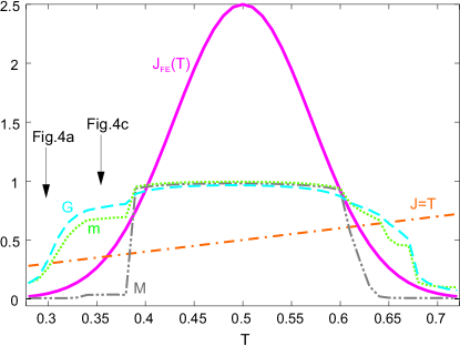
Figure 3: (Color online) Magnetic phase diagram of composite multiferroic vs. temperature $T$ for weak magneto-dipole interaction ($g=0.5$) and zero magnetic anisotropy ($K=0$). All notations are defined in Fig. 1.

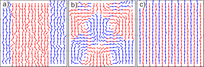
Figure 4: (Color online) Snapshots of single magnetic layer of composite multiferroic. Panel (a) shows the FM state divided into stripe domains appearing due to the interplay of exchange and weak MD interactions. Panel (b) shows the vortex state with magnetic vortices appearing due to strong MD interaction. Panel (c) shows FM chains forming antiferromagnetic pattern appearing at low temperatures and MD interaction being stronger than exchange interaction. Position of panels (a) and (c) is shown in Fig. 3 by black arrows.

V.1.2 Weak and moderate magneto-dipole (MD) interaction

The long-range MD interaction competes with intergrain exchange interaction suppressing the FM state in the system. Figure 3 shows the case of weak MD interaction with the dipole constant, $g=0.5$. This value of $g$ is typical for Fe grains with size $a=4$ nm, where $g=(2.2\mu_{\mathrm{B}}V/\lambda^{3}_{\mathrm{Fe}})^{2}/a^{3}\approx 50$ K, $\lambda_{\mathrm{Fe}}=0.28$ nm is the Fe lattice parameter. Tiago et al. (2006) For these parameters the FM region exists. However, the MD interaction reduces the size of FM state and leads to the formation of domains in the system (see the left panel in Fig. 4). Above the FM region the SPM state appears, similar to the case of zero MD interaction, meaning that the thermal fluctuations exceed the exchange and MD interactions. Below the FM region the thermal fluctuations exceed the exchange interaction but not the MD interaction. As a result the antiferromagnetic stripes appear at low temperatures, $T<0.35$ (see panel (c) in Fig. 4). The transition to stripe structure occurs via formation of large antiferromagnetic domains with temperature dependent sizes.

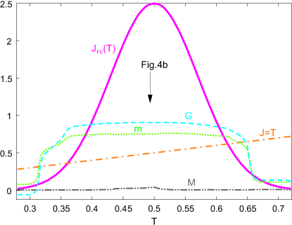
Figure 5: (Color online) Magnetic phase diagram of composite multiferroic vs. temperature $T$ for intermediate magneto-dipole interaction $g=2.0$ and zero magnetic anisotropy ($K=0$). All notations are defined in Fig. 1.

V.1.3 Strong magneto-dipole (MD) interaction

For strong MD interaction, $g\geq 2.0$, the uniform FM state does not appear in the system (see Fig. 5). However, the long-range magnetic correlations are still exist in the system close to $\operatorname{\mathit{T}_{\mathrm{\scriptscriptstyle C}}^{\mathrm{\scriptscriptstyle FE}}}$. For such a strong MD interaction the vortex-like structure appears in the system (see the central snapshots in Fig. 4(b)). The vortex structure transforms into the stripe structure outside the $\operatorname{\mathit{T}_{\mathrm{\scriptscriptstyle C}}^{\mathrm{\scriptscriptstyle FE}}}$ region. For strong MD interaction the SPM state does not appear for temperatures above and below $\operatorname{\mathit{T}_{\mathrm{\scriptscriptstyle C}}^{\mathrm{\scriptscriptstyle FE}}}$, instead the stripe structure appears in these regions. At higher temperatures the stripe structure transforms into SPM state due to thermal fluctuations.

The MD interaction grows with particle volume as $V^{2}$. For Fe grains of size $6$nm and interparticle distance $1$nm the dipole constant is $g\approx 230$ K. This value of MD interaction equals to the peak value of exchange interaction. The exchange interaction grows with grain surface as $V^{2/3}$ and it is intergrain distance dependent.

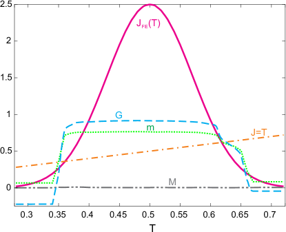
Figure 6: (Color online) Magnetic phase diagram of composite multiferroic vs. temperature $T$ for strong magneto-dipole interaction, $g=5.0$, and zero magnetic anisotropy, $K=0$. All notations are defined in Fig. 1.

Figure 6 shows the case of strong MD interaction with dipole constant $g=5$ being twice larger than the peak value of the exchange interaction. This case is typical for $10$nm $Fe$ grains with MD constant $g$ exceeding the room temperature. Even in this case the FM domains exist in the vicinity of the FE Curie point. The FM state in the vicinity of the FE phase transition is robust against the MD interaction leading to the unusual magnetic phase diagram of composite multiferroics due to ME coupling of ferroelectric and magnetic subsystems.

V.2 Influence of magnetic anisotropy on the magnetic phase diagram of composite multiferroics

In this subsection we discuss the influence of magnetic anisotropy on the magnetic phase diagram of composite multiferroics. The magnetic anisotropy in granular materials is much stronger than in bulk magnets due to surface and shape anisotropy. Liou and Chien (1988); Gong et al. (1991) It plays an important role in formation of magnetic state of granular magnets. The magnetic relaxation time in the system of non-interacting particles exponentially depends on the ratio of anisotropy energy and temperature, $\tau_{\mathrm{r}}\sim\exp(K/(k_{\mathrm{B}}T))$. At low temperatures the relaxation time becomes larger than the characteristic measurement time. At these temperatures the measured magnetic properties are the properties of non-equilibrium or “blocked” state. The temperature hysteresis of magnetic properties is the signature of “blocking” phenomenon. The Monte-Carlo (MC) calculations in some way are similar to real experiment: simulations start with a certain non-equilibrium state and the system “relaxes” to the equilibrium state via discrete steps during the simulations. If number of MC steps $N_{\mathrm{MC}}$ (which can be associated with measurement time if the attempt frequency of the system is known) exceeds a certain value $N_{\mathrm{r}}$ (which can be associated with relaxation time $\tau_{\mathrm{r}}$) then the system relaxes to the equilibrium state during simulations. In the opposite case, the system is locked into some non-equilibrium magnetic state.

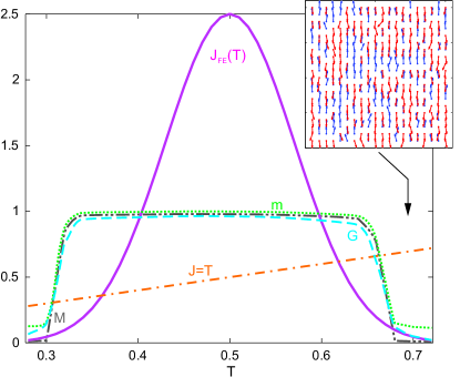
Figure 7: (Color online) Magnetic phase diagram of composite multiferroic vs. temperature $T$ for zero magneto-dipole interaction and strong magnetic anisotropy ($K=6.0$). Insert: Snapshot of a single magnetic layer of composite multiferroic with disordered magnetic state due to strong anisotropy. Black arrow indicates the position of this snapshot on phase diagram. All notations are defined in Fig. 1.

Figure 7 shows the magnetic behavior of granular multiferroics with strong anisotropy, $K=6.0$. This anisotropy is twice larger than the peak value of the exchange interaction. This situation is realized for $6$ nm Fe grains with anisotropy constant $K=0.8\cdot 10^{-6}$ erg/cm³. Gong et al. (1991) Figure 7 coincides with mean-field theory, where FM state exists in the vicinity of the FE phase transition and the disordered state appears away from $\operatorname{\mathit{T}_{\mathrm{\scriptscriptstyle C}}^{\mathrm{\scriptscriptstyle FE}}}$. The only difference with mean field theory is related to the fact that magnetic moments in the disordered state have only two possible directions along the anisotropy axis (see inset in Fig. 7).

For zero MD interaction the MC results do not depend on the initial state of the system. We use two different approaches for MC calculations, see the details in the Appendix: 1) The starting configuration is the FM alignment along the z-direction at the initial temperature point. After a certain number of MC steps the resulting spin configuration is used for the next temperature point. 2) The starting configuration is the disordered state at each temperature point. In addition, we change the direction of temperature evolution and the number of MC steps. Both approaches lead to the same results without hysteresis behavior. Thus, we conclude that in our modelling $N_{\mathrm{MC}}\gg N_{\mathrm{r}}$. And the magnetic anisotropy alone does not qualitatively change the magnetic phase diagram of composite multiferroics and it does not lead to the suppression of ME effects in the system.

V.3 Hysteresis behavior of composite multiferroics with strong magnetic anisotropy and magneto-dipole interaction

In this subsection we discuss the influence of strong magnetic anisotropy and MD interaction on the phase diagram of composite multiferroics and show that these interactions lead to new features. We use the following approach: 1) We move from high to low temperatures starting from the FM state at initial temperature $T=0.72$. At each next temperature point we begin with the final state of the previous temperature point. 2) We move from low $T=0.28$ to high $T=0.72$ temperatures with the initial state corresponding to the FM state. Results are shown in Fig. 8.

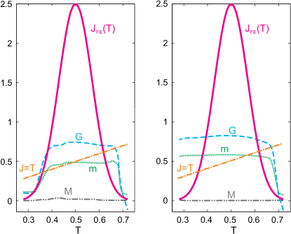
Figure 8: (Color online) Temperature hysteresis of composite multiferroic. Left and right panels correspond to the case of increasing and decreasing temperature, respectively.

The presence of MD interaction increases the blocking temperature leading to larger magnetic relaxation time, $\tau_{\mathrm{r}}$. Liua and Bertram (2001); Chantrell et al. (2000) However, this is not the case for our system. To understand the nature of hysteresis in composite multiferroics consider the starting point $T=0.28$ in the “warming” case, left panel, with the uniform FM state as the initial state. The final state at this temperature obtained after MC simulations is the disordered (SPM) state. The system relaxes from FM to SPM state in the process of calculations. Therefore neither magnetic anisotropy nor the MD interaction produce “blocking” in the system at these temperatures.

However, if we move from high to low temperatures the relaxation to the SPM state does not occur at temperature $T=0.28$. The reason for the cooling process is related to the fact that one needs to pass the peak in the exchange interaction at temperature $T=0.5$ where multiple inhomogeneous FM state with domains of different orientations is formed. Around $T=0.5$ the average magnetization (the red curve) is zero. But the cell averaged magnetization is finite meaning that the system is divided into domains of opposite magnetization. These domains occur due to the interplay of exchange and MD interactions. This multidomain state is robust against thermal fluctuations for $T<0.5$ even for zero exchange interaction. This is in contrast to the uniform FM state, which can be destroyed in the absence of exchange interaction even at low temperatures. As a result the magnetization vs. temperature has a hysteresis behavior.

At higher temperature, $T\approx 0.7$, the multidomain state is unstable against thermal fluctuations at these temperatures and the hysteresis behavior is absent.

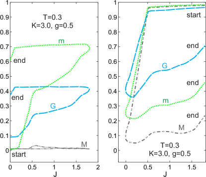
Figure 9: (Color online) Evolution of magnetic phase diagram of composite multiferroic as a function of exchange interaction at fixed temperature.

Figure 9 shows the magnetic phase diagram as a function of exchange constant $J$ at fixed temperature $T=0.3$. On the left panel we increase the exchange constant $J$ starting from zero to a certain high value and decrease it back to zero. The initial spin configuration at $J=0$ is the uniform FM state. On the right panel in Fig. 9 we start with finite value of exchange interaction $J$, decrease it to zero and return back to the same value. Obviously, such a nonmonotonic behavior of exchange interaction occurs with changing the temperature in composite multiferroic. Figure 9 shows the hysteresis behavior caused by the non monotonic change of the intergrain exchange interaction. Similar hysteresis occurs as a function of temperature.

To summarize, the above hysteresis is specific to composite multiferroics - materials with non-monotonic behavior of exchange interaction. The hysteresis is absent for systems with temperature independent exchange interaction. The peculiar feature of this hysteresis is related to the fact that it appears in the vicinity of the FE Curie point.

V.4 Deep in the exchange interaction in the vicinity of FE Curie point

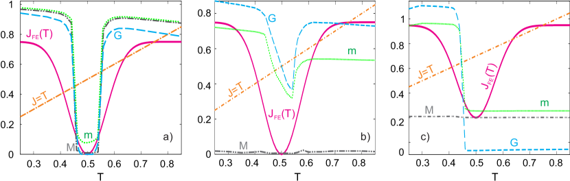
Figure 10: (Color online) Magnetic phase diagram of composite multiferroic vs. temperature $T$ for the case of deep in the exchange interaction in the vicinity of the FE Curie point. Panel (a): zero magneto-dipole (MD) interaction ($g=0.0$) and zero magnetic anisotropy ($K=0.0$). Panel (b): moderate MD interaction ($g=1.0$) and zero magnetic anisotropy ($K=0.0$). Panel (c): strong MD interaction ($g=1.0$) and zero magnetic anisotropy ($K=0.0$). Solid (red) line shows the temperature dependence of intergrain exchange interaction, $J(T)$. Straight dash dotted (orange) line stands for temperature $T$. Gray dash dotted and green dotted lines show the average magnetization $M(T)$ and cell averaged magnetization $m(T)$, respectively. Blue dashed line shows the nearest neighbour correlation function $G$.

The intergrain exchange interaction has either peak or deep in the vicinity of FE Curie point depending on the system parameters. Udalov et al. (2014) Here we study the situation with deep in the exchange interaction in the vicinity of the FE Curie point. Figure 10a shows the case of zero MD interaction and zero anisotropy with the following parameters: the deep is $J_{0}=0.75$, $\operatorname{\Delta\mathit{T}^{\mathrm{\scriptscriptstyle FE}}}=0.07$, and $\operatorname{\mathit{T}_{\mathrm{\scriptscriptstyle C}}^{\mathrm{\scriptscriptstyle FE}}}=0.5$. In this case the Monte-Carlo simulations and the mean field approximation coincide. For chosen parameters the exchange interaction exceeds the temperature in the whole range except the close vicinity of FE transition, where exchange interaction is small and the system is in the SPM state. Outside this region the system is in the FM state. A single domain state with two magnetic phase transitions is realized for zero MD interaction.

A moderate MD interaction leads to the domains formation in the FM phase and to the formation of magnetic vortices in the transition regions. Figure 10b shows this behavior for dipole constant $g=0.5$.

Strong MD interaction ($g=5.0$) leads to the suppression of the FM state at high temperatures, see Fig. 10c. Here the AFM stripe structure appears instead of FM ordering. At low temperatures the FM state exists. Therefore in the case of deep in the exchange interaction the MD interaction leads to the suppression of high temperature magnetic phase transition in contrast to the case of peak in the exchange interaction. At higher temperatures, $T>1$, the AFM state is suppressed due to thermal fluctuations.

V.5 Applicability of results

Here we discuss the applicability of our approach. First, we study the case of regular magnetic array with fixed intergrain distances. In real materials this distance fluctuates leading to the dispersion of MD and exchange interactions.

Second, we consider 3D multiferroic materials which produced via bottom-up method. A different top-down fabrication, based on layer by layer growth, is used to produce a single layer of magnetic grains. In 2D systems the influence of MD interaction on the magnetic phase diagram is different from 3D case. This situation requires further investigation.

VI Conclusion

We studied the competition of magneto-dipole, anisotropy and exchange interactions in composite three dimensional multiferroics – materials with magnetic grains embedded into FE matrix. The peculiarity of composite (or granular) multiferroics is related to the fact that interparticle interaction is affected by the FE matrix. Granular multiferroics show the magneto-electric coupling effect. Using Monte Carlo simulations we showed that magneto-dipole interaction does not suppress the ferromagnetic state caused by the interaction of the ferroelectric matrix and magnetic subsystem. Thus, MD interaction does not suppress the ME effect in granular multiferroics. However, the presence of magneto-dipole interaction influences the order-disorder transition: depending on the strength of magneto-dipole interaction the transition from the FM to the SPM state is accompanied either by creation of vortices or domains of opposite magnetization.

We showed that “blocking phenomenon” appears at finite magnetic anisotropy and finite MD interaction. The temperature hysteresis loop occurs due to non-monotonic behavior of exchange interaction vs. temperature. The origin of this hysteresis is related to the presence of stable magnetic domains which are robust against thermal fluctuations.

VII Acknowledgements

We thank Shauna Robbennolt and Sarah Tolbert for useful discussions. I. B. was supported by NSF under Cooperative Agreement Award EEC-1160504, NSF Award DMR-1158666 and the U.S. Civilian Research and Development Foundation (CRDF Global). A. B. and N. C. are grateful to Russian Academy of Sciences for the access to JSCC and “Uran” clusters and Kurchatov center for access to HCP supercomputer cluster. A. B. acknowledges support of the Russian foundation for Basic Research (grant No. 13-02-00579). N. C. acknowledges Laboratoire de Physique Théorique, Toulouse and CNRS for hospitality and Russian Fundamental Research foundation (grant No. 14-12-01185) for support of supercomputer simulations.

Appendix A Calculation procedure

We use classical Monte Carlo (MC) simulations and the standard Metropolis algorithm to model magnetic properties of the system. Landau and Binder (2000); Kretschmer and Binder (1979); Binder and Landau (1976); Binder and Rauch (1969); Landau and Binder (1981); Petracic et al. (2006) We consider $L\times L\times L$ ($L=20$) cubic lattice with periodic boundary conditions. To efficiently evaluate the long-range MD interaction in systems with relatively small number of particles (as, for example, $L=5,6,7$ considered in Ref. Kretschmer and Binder (1979); Kechrakos and Trohidou (1998b)) one has to implement Ewald summation technique. Allen and Tildesley (1987); Z.Wang and Holm (2001) We account the MD interaction by direct summation in the real space applying the minimum image convention. Allen and Tildesley (1987) In terms of the range of the interaction that have been taken into account, this scheme is equivalent to the fast Fourier transform method used for micromagnetic simulations. Hinzke and Nowak (2000); Yuan and Bertram (1992)

We use the FM state ordered along the $z$-direction, ${\bf S}_{i}={\bf e}_{z}$, as an initial spin configuration for simulating at the first temperature point. The resulting spin state is used as an initial state for the next temperature point and so on. To study hysteresis effects we make two passages: first, we start with low temperature and increase the temperature during our calculations; second, we do the opposite.

One MC step consists of $L\times L\times L$ consecutive changes in the lattice spin orientations. We calculated the change in the energy of the system $\Delta{\cal H}$: if change is negative, $\Delta{\cal H}\leq 0$, a new state is accepted; if change is positive, $\Delta{\cal H}>0$, the new state is accepted with probability $e^{-\Delta{\cal H}/T}$. In our simulations we use $N_{MC}=12000$ MC steps per spin and study 60 samples in every 200 MC steps to calculate thermal properties. To check the stability of final configuration on the number of MC steps we increased the number of MC steps five times (up to $N_{MC}=6\cdot 10^{4}$) and find no difference in the resulting state.

We generate the update in spin directions using two ways. First, the spin orientations were distributed uniformly over the unit sphere’s surface Z.Wang and Holm (2001)

$$\cos\theta_{i}=\xi,\quad\varphi_{i}=\pi\xi^{\prime},$$ (11)

where $\xi,\xi^{\prime}$ are some random numbers from the interval $(-1,1)$. This algorithm becomes inefficient at low temperatures or strong anisotropy. In this case the majority of randomly chosen spin directions has to be rejected due to large energy change $\Delta{\cal H}$. We use such an update to check the results of the second algorithm with tuned step of change in the spin direction.

Our main algorithm for spin change was an algorithm where a new spin direction is chosen within a small angle near a given spin ${\bf S}_{i}$ Serena et al. (1993b). First, a random unit vector ${\bf w}$ perpendicular to the chosen spin ${\bf S}_{i}$ is generated. Then new trial configuration is chosen as

$${\bf S}^{\prime}_{i}=\cos\theta_{i}{\,}{\bf S}_{i}+\sin\theta_{i}{\,}{\bf w},$$ (12)

where $\theta_{i}$, the rotation angle from ${\bf S}_{i}$ to ${\bf S}^{\prime}_{i}$, is chosen according to

$$\cos\theta_{i}=1+\xi(\cos\theta_{max}-1),$$ (13)

$\xi$ is a random number varying in the interval $(0,1)$, the angle $\theta_{max}$ is a maximum allowed amplitude for the change of the polar angle $\theta_{i}$ of the initial spin ${\bf S}_{i}$, $0<\theta_{max}\leqslant\pi$. The new spin direction ${\bf S}^{\prime}_{i}$ lies within a cone around the initial direction with aperture angle $2\theta_{max}$ and all the directions inside this cone can be reached with the same probability Serena et al. (1993b). The value of $\theta_{max}$ is adjusted after one full MC sweep over the lattice to keep, when possible, the number of accepted spin changes around $\sim 50\%$. Also we kept the lower bound for $\theta_{max}\gtrsim\pi/6$ to prevent too small MC moves which are inefficient to thermalize the system.

This algorithm is not valid at low temperatures Petracic et al. (2006) or strong anisotropy, $K\gg 1$, when the system tends to the Ising limit which does not allow the spin flips. We improve the situation allowing spins to flip with a certain small probability ($\lesssim 0.1-0.2$). With this modification we reproduce the correct values of the critical temperature $T_{c}$ for the Heisenberg, $T_{c}\simeq 1.44$, Lau and Dasgupta (1989); Holm and Janke (1993); Peczak et al. (1991); Chen et al. (1993); Watson et al. (1969); Landau and Binder (1981); Binder and Rauch (1969); Binder and Landau (1976); Watson et al. (1969) and the Ising, $T_{c}\simeq 4.51$, models. Binder (2001)

References

- Cheong and Mostovoy (2007) S.-W. Cheong and M. Mostovoy, Nature materials 6, 13 (2007).
- Khomskii (2006) D. I. Khomskii, J. Mag. Magn. Mater. 306, 1 (2006).
- Katsura et al. (2005) H. Katsura, N. Nagaosa, and A. V. Balatsky, Phys. Rev. Lett. 95, 057205 (2005).
- Mostovoy (2006) M. Mostovoy, Phys. Rev. Lett. 96, 067601 (2006).
- Kimura (2007) T. Kimura, Annu. Rev. Mater. Res. 37, 387 (2007).
- Ederer and Spaldin (2005) C. Ederer and N. A. Spaldin, Phys. Rev. B 71, 060401(R) (2005).
- Kornev et al. (2007) I. A. Kornev, S. Lisenkov, R. Haumont, B. Dkhil, and L. Bellaiche, Phys. Rev. Lett. 99, 227602 (2007).
- Fiebig (2005) M. Fiebig, J. Phys. D: Appl. Phys. 38, R123 (2005).
- Eerenstein et al. (2006) W. Eerenstein, N. D. Mathur, and J. F. Scott, Nature 442, 759 (2006).
- Ramesh and Spaldin (2007) R. Ramesh and N. A. Spaldin, Nature Mat. 6, 21 (2007).
- Sone et al. (2012) K. Sone, S. Sekiguchi, H. Naganuma, T. Miyazaki, T. Nakajima, and S. Okamura, J. Appl. Phys. 111, 124101 (2012).
- Udalov et al. (2014) O. G. Udalov, N. M. Chtchelkatchev, and I. S. Beloborodov, Phys. Rev. B 89, 174203 (2014).
- Udalov et al. (2015) O. G. Udalov, N. M. Chtchelkatchev, and I. S. Beloborodov, J. Phys.: Condens. Matter 27, 186001 (2015).
- Woi nska et al. (2013) M. Woi nska, J. Szczytko, A. Majhofer, J. Gosk, K. Dziatkowski, and A. Twardowski, Phys. Rev. B 88, 144421 (2013).
- Liua and Bertram (2001) A. D. Liua and H. N. Bertram, J. Appl. Phys. 89, 2861 (2001).
- Gong et al. (1991) W. Gong, H. Li, Z. Zhao, and J. Chen, J. Appl. Phys. 69, 5119 (1991).
- Laurent et al. (1989) C. Laurent, D. Mauri, E. Kay, and S. S. P. Parkin, J. Appl. Phys. 65, 2017 (1989).
- Liou and Chien (1988) S. H. Liou and C. L. Chien, J. Appl. Phys. 63, 4240 (1988).
- Bedanta and Kleemann (2009) S. Bedanta and W. Kleemann, J. Phys. D: Appl. Phys. 42, 013001 (2009).
- Chantrell et al. (2000) R. W. Chantrell, N. Walmsley, J. Gore, and M. Maylin, Phys. Rev. B 63, 024410 (2000).
- Kechrakos and Trohidou (1998a) D. Kechrakos and K. N. Trohidou, Phys. Rev. B 58, 12169 (1998a).
- Petracic et al. (2004) O. Petracic, A. Glatz, and W. Kleemann, Phys. Rev. B 70, 214432 (2004).
- Kleemann et al. (2001) W. Kleemann, O. Petracic, C. Binek, G. N. Kakazei, Y. G. Pogorelov, J. B. Sousa, S. Cardoso, and P. P. Freitas, Phys. Rev. B 63, 134423 (2001).
- Petracic et al. (2006) O. Petracic, X. C. amd S. Bedanta, W. Kleemanna, S. Sahoo, S. Cardoso, and P. P. Freitas, J. Mag. Magn. Mater. 300, 192 (2006).
- Sankar et al. (2000) S. Sankar, D. Dender, J. A. Borchers, D. J. Smith, R. W. Erwin, S. R. Kline, and A. E. Berkowitz, J. Mag. Magn. Mater. 221, 1 (2000).
- El-Hilo et al. (1998) M. El-Hilo, R. W. Chantrell, and K. O Grady, J. Appl. Phys. 84, 5114 (1998).
- Chien (1988) C. L. Chien, J. Appl. Phys. 69, 5267 (1988).
- Ayton et al. (1995) G. Ayton, M. J. P. Gingras, and G. N. Patey, Phys. Rev. Lett. 75, 2360 (1995).
- Ravichandran and Bagchi (1996) S. Ravichandran and B. Bagchi, Phys. Rev. Lett. 76, 644 (1996).
- Mamiya et al. (1999) H. Mamiya, I. Nakatani, and T. Furubayashi, Phys. Rev. Lett. 82, 4332 (1999).
- Djurberg et al. (1997) C. Djurberg, P. Svedlindh, P. Nordblad, M. F. Hansen, F. Bodker, , and S. Morup, Phys. Rev. Lett. 79, 5154 (1997).
- Sahoo et al. (2003) S. Sahoo, O. Petracic, W. Kleemann, P. Nordblad, S. Cardoso, and P. P. Freitas, Phys. Rev. B 67, 214422 (2003).
- Timopheev et al. (2012) A. A. Timopheev, I. Bdikin, A. F. Lozenko, O. V. Stognei, A. V. Sitnikov, A. V. Los, and N. A. Sobolev, J. Appl. Phys. 111, 123915 (2012).
- Scheinfein et al. (1996) M. R. Scheinfein, K. E. Schmidt, K. R. Heim, and G. G. Hembree, Phys. Rev. Lett. 76, 1541 (1996).
- Kondratyev and Lutz (1998) V. N. Kondratyev and H. O. Lutz, Phys. Rev. Lett. 81, 4508 (1998).
- Bedanta et al. (2007) S. Bedanta, T. Eimuller, W. Kleemann, J. Rhensius, F. Stromberg, E. Amaladass, S. Cardoso, and P. P. Freitas, Phys. Rev. Lett. 98, 176601 (2007).
- Atherton and Beattie (1990) D. L. Atherton and J. R. Beattie, IEEE Tran. Magn. 26, 3059 (1990).
- Timopheev et al. (2009) A. A. Timopheev, S. M. Ryabchenko, V. M. Kalita, A. F. Lozenko, P. A. Trotsenko, V. A. Stephanovich, A. M. Grishin, and M. Munakata, J. Appl. Phys. 105, 083905 (2009).
- Wiedwald et al. (2004) U. Wiedwald, M. Cerchez, M. Farle, K. Fauth, G. Schutz, K. Zurn, H.-G. Boyen, and P. Ziemann, Phys. Rev. B 70, 214412 (2004).
- Garcia-Palacios and Lazaro (1998) J. L. Garcia-Palacios and F. J. Lazaro, Phys. Rev. B 58, 14937 (1998).
- Serena et al. (1993a) P. A. Serena, N. Garcia, and A. Levanyuk, Phys. Rev. B 47, 5027 (1993a).
- ElHilo et al. (1994) M. ElHilo, K. O Grady, and R. W. Chantrell, J. Appl. Phys. 76, 6811 (1994).
- Asselin et al. (2010) P. Asselin, R. F. L. Evans, J. Barker, R. W. Chantrell, R. Yanes, O. Chubykalo-Fesenko, D. Hinzke, and U. Nowak, Phys. Rev. B 82, 054415 (2010).
- Atxitia et al. (2010) U. Atxitia, D. Hinzke, O. Chubykalo-Fesenko, U. Nowak, H. Kachkachi, O. N. Mryasov, R. F. Evans, and R. W. Chantrell, Phys. Rev. B 82, 134440 (2010).
- Du et al. (2010) H.-F. Du, W. He, D.-L. Sun, Y.-P. Fang, H.-L. Liu, X.-Q. Zhang, and Z.-H. Cheng, Appl. Phys. Lett. 96, 132502 (2010).
- Matsubara and Itoya (1993) F. Matsubara and T. Itoya, Progress of Theoretical Physics 90, 471 (1993).
- Hinzke and Nowak (1999) D. Hinzke and U. Nowak, Computer Physics Communications 121 122, 334 (1999), proceedings of the Europhysics Conference on Computational Physics {CCP} 1998.
- Strukov and Levanyuk (1998) B. A. Strukov and A. P. Levanyuk, Ferroelectric Phenomena in Crystals (Springer, Geidelberg, 1998, 1998).
- Lau and Dasgupta (1989) M. H. Lau and C. Dasgupta, Phys. Rev. B 39, 7212 (1989).
- Holm and Janke (1993) C. Holm and W. Janke, Phys. Rev. B 48, 936 (1993).
- Peczak et al. (1991) P. Peczak, A. M. Ferrenberg, and D. P. Landau, Phys. Rev. B 43, 6087 (1991).
- Chen et al. (1993) K. Chen, A. M. Ferrenberg, and D. P. Landau, Phys. Rev. B 48, 3249 (1993).
- Huth et al. (2014) M. Huth, A. Rippert, R. Sachser, and L. Keller, Mater. Res. Expr. 1, 046303 (2014).
- Tiago et al. (2006) M. L. Tiago, Y. Zhou, M. M. G. Alemany, Y. Saad, and J. R. Chelikowsky, Phys. Rev. Lett. 97, 147201 (2006).
- Landau and Binder (2000) D. P. Landau and K. Binder, A Guide to Monte Carlo Simulations in Statistical Physics (Cambridge University Press, Cambridge, 2000).
- Kretschmer and Binder (1979) R. Kretschmer and K. Binder, Z. Phys. B 34, 375 (1979).
- Binder and Landau (1976) K. Binder and D. P. Landau, Phys. Rev. B 13, 1140 (1976).
- Binder and Rauch (1969) K. Binder and H. Rauch, Z. Phys. 219, 201 (1969).
- Landau and Binder (1981) D. P. Landau and K. Binder, Phys. Rev. B 24, 1391 (1981).
- Kechrakos and Trohidou (1998b) D. Kechrakos and K. N. Trohidou, Phys. Rev. B 58, 12169 (1998b).
- Allen and Tildesley (1987) M. P. Allen and D. J. Tildesley, Computer Simulation of Liquids 1st ed. (Clarendon, Oxforde, 1987).
- Z.Wang and Holm (2001) Z.Wang and C. Holm, J. Chem. Phys. 115, 6351 (2001).
- Hinzke and Nowak (2000) D. Hinzke and U. Nowak, J. Mag. Magn. Mater. 221, 365 (2000).
- Yuan and Bertram (1992) S. W. Yuan and H. N. Bertram, IEEE Trans. Magn. 28, 2031 (1992).
- Serena et al. (1993b) P. A. Serena, N. Garcia, and A. Levanyuk, Phys. Rev. B 47, 5027 (1993b).
- Watson et al. (1969) R. E. Watson, M. Blume, and G. H. Vineyard, Phys. Rev. 181, 811 (1969).
- Binder (2001) K. Binder, Phys. Reports 344, 179 (2001).