Ionization potentials and electron affinities from the extended Koopmans’ theorem in self-consistent Green’s function theory

Abstract

One-body Green’s function theories implemented on the real frequency axis offer a natural formalism for the unbiased theoretical determination of quasiparticle spectra in molecules and solids. Self-consistent Green’s function methods employing the imaginary axis formalism on the other hand can benefit from the iterative implicit resummation of higher order diagrams that are not included when only the first iteration is performed. Unfortunately, the imaginary axis Green’s function does not give direct access to the desired quasiparticle spectra, which undermines its utility. To this end we investigate how reliably one can calculate quasiparticle spectra from the Extended Koopmans’ Theorem (EKT) applied to the imaginary time Green’s function in a second order approximation (GF2). We find that EKT in conjunction with GF2 yields IPs and EAs that systematically underestimate experimental and accurate coupled-cluster reference values for a variety of molecules and atoms. This establishes that the EKT allows one to utilize the computational advantages of an imaginary axis implementation, while still being able to acquire real axis spectral properties. Because the EKT requires negligible computational effort, and can be used with a Green’s function from any level of theory, we conclude that it is a potentially very useful tool for the systematic study of quasiparticle spectra in realistic systems.

I Introduction

Finding practical and principled methods to numerically solve the many-electron Schrödinger equation for realistic chemical systems is a substantial problem that has been attacked by the scientific community for more than five decades now. Though diverse in approach, the bulk of these methods can be classified as either being based on the single-particle density $\rho(\mathbf{r})$ or the many-body wavefunction $\Psi$. Kohn-Sham density functional theory (DFT)Hohenberg and Kohn (1964); *PhysRev.140.A1133; Parr and Yang (1989) and the coupled cluster theory (CC)Coester and Kümmel (1960); Cizek (1991); Bartlett and Musiał (2007) are two remarkably successful examples of these former and latter categories. Despite their merits and widespread use, by now it’s become well established these classes of methods have their respective limitations that are unlikely to be overcome in the near future. For instance CC theory, though being the gold standard for weakly correlated systems, cannot successfully account for multi-reference effects present in strongly correlated molecules and solids, and its computational scaling seems to limit use for large systems. DFT in contrast is computationally affordableScuseria (1999), but is plagued by a lack of systematic approaches to improve functionalsBurke (2012), as well as the fact that many approximate functionals can give a frustratingly non-uniform performance across different systems and properties. This problem is exemplified for metal oxides, where even within the same system different DFT approximations are required for different propertiesBredow and Gerson (2000); de P. R. Moreira et al. (2002). Furthermore, as spectral properties are concerned, even with the exact functional the Kohn-Sham (KS) gap cannot provide a theoretically sound approximation to the fundamental gapPerdew and Levy (1983); Perdew (1985); Stoudenmire et al. (2012); Baerends et al. (2013).

Approaches based on the self-consistent single-particle Green’s function, $G(\omega)$, are an attractive alternative with strengths and weaknesses that are complementary to density and wavefunction-based methods. Similar to DFT, Green’s function methods can be implemented in a blackbox manner in the atomic orbital (AO) basisFoerster et al. (2011); Caruso et al. (2013); Phillips and Zgid (2014); Koval et al. (2014), and typically will feature lower order polynomial scaling than wavefunction-based methods such as CCSD (coupled cluster singles doubles). Additionally, Green’s function methods offer a natural language for embedding approaches since the Green’s function can be partitioned among subsystems (similar to the density).

Because of the need to evaluate $G(\omega_{n})$ on a numerical grid, $\omega_{n}$, Green’s function based approaches can be broadly grouped into two classes:

Greens functions on the imaginary (Matsubara grid) axis describe a grand canonical ensemble and can be used to calculate temperature dependent quantities such as the free energy, specific heat, etc. A Green’s function of the imaginary axis is a smooth function, with only a single pole near zero that is not accessed for any finite temperature larger than zero. Consequently, the imaginary axis formulation is a natural choice for any self-consistent approach where the Green’s function is expressed as a functional of the self-energy, $G[\Sigma(\omega)]$, and where at self-consistency infinite classes of diagrams can be included due to the implicit resummation. A result of this diagrammatic resummation is that these approachesPhillips and Zgid (2014); Dahlen and van Leeuwen (2005); Stan et al. (2009); Caruso et al. (2013) give finite results in strongly correlated cases when other methods such as truncated CC or MP2 (second order Møller-PlessetMøller and Plesset (1934)) would diverge pathologically.

Greens functions on the real frequency axis are more commonly employed in quantum chemistry for zero-temperature calculations. The single-particle Green’s function on the real axis has multiple poles which correspond to ionization potential (IP) and electron affinity (EA) peaks Hedin (1965); Albertsen and Jørgensen (1979); B. and Öhrn (1981); Schirmer et al. (1983); Cederbaum (1990); Massidda et al. (1995); *Massidda_MetalOxide_GW_prb_1997; Ku and Eguiluz (2002); Rostgaard et al. (2010); Ortiz (2013) in the photoelectron spectrum. The two-particle real-axis Green’s function is capable of describing optical/neutral excitations. Performing the calculation self-consistently (where $G[\Sigma(\omega)]$ is evaluated as a functional of $\Sigma(\omega)$) is notoriously difficult on the real axis, because the series of poles in the real-axis Green’s function requires a non-uniform grid that can change between iterations.

The real and imaginary axis formalisms should be treated as complementary but requiring the development of different tools in order to evaluate accurate Green’s functions. The interesting question that arises is if one can use an approach that has “the best of both worlds”; that is, to calculate the Green’s function on the imaginary axis in order to take advantage of the efficient self-consistency, and to subsequently employ the imaginary axis solution to calculate spectra on the real axis.

One of the routes to obtaining a real axis Green’s function from the imaginary axis data is through the process of analytic continuation Gunnarsson et al. (2010); Jarrell and Gubernatis (1996); Gubernatis et al. (1991). This procedure is known to suffer from several problems, namely it cannot recover sharp spectral features, frequently is problematic in recovering fundamental gap edges, and is very sensitive to the initial imaginary axis data.

Here, we attempt to examine an alternative answer to this problem. We will investigate how accurately and reliably one can calculate quasiparticle spectra from the extended Koopman’s theorem (EKT)Smith and Day (1975); *EKT_Original_II; Pickup (1975); Katriel and Davidson (1980); Matos and Day (1987); Morrison (1992); Sundholm and Olsen (1993); Morrison and Ayers (1995); Cioslowski et al. (1997); Olsen and Sundholm (1998); Pernal and Cioslowski (2001); Ernzerhof (2009); Bozkaya (2013, 2014) starting from self-consistent Green’s function many-body theoryPhillips and Zgid (2014); Dahlen and van Leeuwen (2005); Stan et al. (2009) in an imaginary axis implementation. The EKT is valuable because it allows one to obtain, in principle, both IPs and EAs from a single electronic structure calculation on the neutral system. Similar to population analysisReed et al. (1985), the actual EKT procedure itself takes place in a simple post-calculation analysis, utilizing the density matrix and other quantities obtained by the preceding correlated method. As a result the EKT can be implemented in a blackbox manner, requires only a negligible fraction of time, and is not tied to any particular level of theory. Despite its simplicity, most of the efforts so far seem to have focused on its application for calculating IPs onlySmith and Day (1975); *EKT_Original_II; Pickup (1975); Morrison (1992); Morrison and Liu (1992); Cioslowski et al. (1997); Pernal and Cioslowski (2005); Dahlen and van Leeuwen (2005); Stan et al. (2009); Bozkaya (2013). While an interesting benchmark of the EKT for EAs has appeared recentlyBozkaya (2014), in that work Bozkaya actually obtained the EA indirectly by calculating the IP of the anion. In contrast, in this work we will calculate IPs and EAs from the neutral system via the EKT. As far as we are aware, EAs typically have not been calculated in this manner.

While the EKT has usually been formulated in terms of a generalized FockianCioslowski et al. (1997) that is evaluated using methods such as configuration interaction (CI) or MP2, in this work we approach EKT with the machinery of second order Green’s function theory (GF2) Phillips and Zgid (2014); Dahlen and van Leeuwen (2005). As shown by Dahlen, Stan, and van LeeuwenDahlen and van Leeuwen (2005); Stan et al. (2009), via EKT it is possible to calculate both IPs and EAs from the imaginary time Green’s function of the neutral system alone. This is potentially very useful for studying the spectral properties of extended systems, because it would circumvent the numerically ill defined step of analytic continuation to the real axis. While their initial results for IPs obtained with GF2 and GW were promising, here we intend to examine GF2’s performance for IPs and EAs for a wider group of atoms and small molecules.

II Theoretical calculations of ionization potentials and electron affinities

To make this work self-contained, here we briefly review some of the different strategies that have been utilized to calculate IPs, EAs, and the fundamental gap $E_{\scriptstyle g}=\textnormal{IP}-\textnormal{EA}$, using wavefunction theory, DFT, many-body theory, and combinations thereof. Naively, the simplest strategy for obtaining these quantities would be by energy differences of the neutral and charged cation/anion systems. However this is fundamentally problematic for periodic boundary-conditions (PBC) calculations of materials in the solid-state, where it would imply the presence of an infinite amount of unbalanced charge in the crystal. Even for finite systems, careful early CI studiesSasaki and Yoshimine (1974); *Sasaki_EA_PRA_1974_ii; Feller and Davidson (1989); Kendall et al. (1992) found that obtaining accurate EAs from energy-differences was particularly challenging because the correlation energy of the anion could converge appreciably slower than that of the neutral system. Additionally, methods with significant amounts of self-interaction error (such as approximate DFT) may not be able to bind some anions at allRösch and Trickey (1997); Galbraith and Schaefer (1996); Jensen (2010).

For these reasons, significant interest has been placed in obtaining IPs and EAs directly from a single calculation on the neutral system. An exemplar for this is offered by the equation of motion coupled cluster theory (EOM-CC)Emrich (1981); Sekino and Bartlett (1984); Geertsen et al. (1989); Stanton and Bartlett (1993); Krylov (2008) for electron attachment and removalNooijen and Bartlett (1995, 1997); Musial et al. (2003); Musial and Bartlett (2003, 2004); Kamiya and Hirata (2007); Musial and Bartlett (2007). EOM-CC is a generalization of the original coupled cluster theory to charged and neutral excitations, and thus largely inherits the advantages and disadvantages of the CC method: if a single determinant description is valid, and the calculation not prohibitively expensive, one can expect very accurate results. Closely related to IP/EA-EOM-CC is the coupled cluster Green’s function method of Nooijen and SnijdersNooijen and Snijders (1992); *Marcel_CC_GreensFunction_ijqc_1993; *Marcel_gf2_CC_IP_jcp_1995, that again will bear some of the advantages and disadvantages of the underlying CC theory.

In the same spirit, Green’s function (also called electron propagator) methods such as the n^th-order Algebraic Diagrammatic Approximation (ADC(n))Schirmer (1982); Schirmer et al. (1983); Tarantelli and Cederbaum (1989) and various self-energy approximationsFlores-Moreno et al. (2010) have found regular use for the accurate, direct determination of IPs and EAs in finite systemsCederbaum (1973); B. and Öhrn (1981); Ortiz (1988, 1989); Cederbaum (1990); Ortiz (1996, 1998); Deleuze et al. (1999); Seabra et al. (2004); Trofimov and Schirmer (2005); Starcke et al. (2006); Müller and Cederbaum (2006). Typically the underlying scheme in these methods is the iterative diagonalization of the self-energy on the real axis in the molecular orbital (MO) basis, $\mathbf{\Sigma}(\lambda_{i})\mathbf{c}_{i}=\lambda_{i}\mathbf{c}_{i}$, until one converges to a given IP, $\lambda_{i}$. As such, this is quite distinct from the fully self-consistent Green’s function implementations in the local AO basis that have appeared recentlyCaruso et al. (2013); Koval et al. (2014); Phillips and Zgid (2014) and that we are considering presently in this work.

A theoretically not fully justified however computationally cheap strategy for directly obtaining quasiparticle spectra would be to simply perform a DFT calculation on the neutral system, and then interpret the resulting KS eigenvalues as IPs and EAs. Unfortunately, as previously mentioned there is no rigorous theoretical grounding for such a procedurePerdew and Levy (1983); Perdew (1985); Godby et al. (1986); Grüning et al. (2006); Baerends et al. (2013): even if the exact functional were used, while the highest occupied KS orbital eigenvalue would be the negative of the ionization potential, the KS gap $E^{\scriptscriptstyle KS}_{\scriptstyle g}$ would still differ from the exact fundamental gap $E_{\scriptstyle g}$ by an amount equalling the derivative discontinuity of the exchange-correlation (XC) potential, $E_{\scriptstyle g}=E^{\scriptscriptstyle KS}_{\scriptstyle g}+\Delta_{\scriptscriptstyle XC}$. As shown recently with stretched hydrogen chains, when strong correlation is present the derivative-discontinuity $\Delta_{\scriptscriptstyle XC}$ can actually become the dominant contribution to $E_{\scriptstyle g}$Stoudenmire et al. (2012). If one disregards this principled objection, in practice the KS gap still underpredicts the fundamental gap significantly, which is partly a consequence of the fractional-charge error in approximate density functionalsPerdew and Zunger (1981); Perdew et al. (1982); Ruzsinszky et al. (2006); Sànchez et al. (2006); Cohen et al. (2008).

Because Hartree-Fock and KS DFT tend to have opposing fractional-charge errors, these methods will typically overestimate and underestimate the fundamental gap, respectively. For this reason there will almost always be a system-dependent empirical hybrid functional that will describe the fundamental gap wellBredow and Gerson (2000); de P. R. Moreira et al. (2002); Moussa et al. (2012) when calculated in the Generalized Kohn-Sham (GKS)Seidl et al. (1996) formalism as band energy-differences. From this standpoint it’s understandable why the HSE functionalHeyd et al. (2003); *Heyd:2004ud has enjoyed so much success for many insulators and semiconductorsHeyd et al. (2005); Brothers et al. (2008); Henderson et al. (2011), though it’s been remarked the HSE gap will tend to match the optical gap better than the fundamental gapBrothers et al. (2008); Henderson et al. (2011).

Because of these fundamental issues with the KS eigenvalues, a very commonly used strategy has been to perform “one-shot” corrections to the DFT spectra with the $G_{0}W_{0}$ approximationHedin (1965); Hybertsen and Louie (1986); Onida et al. (2002). From a purely pragmatic viewpoint the resulting quasiparticle spectra can be much improved with respect to experiment. However from a principled standpoint this is not entirely satisfying because it is highly dependent on the starting DFT solution which is functional dependent. Because of this, the $G_{0}W_{0}$ results can vary significantly depending on the combination of system and density functional usedFuchs et al. (2007); Blase et al. (2011); Marom et al. (2011, 2011); Liao and Carter (2011); Toroker et al. (2011); Isseroff and Carter (2012); Marom et al. (2012); Körzdörfer and Marom (2012); Bruneval and Marques (2013). To highlight one such example, for hematite ($\alpha$-Fe₂O₃) the $G_{0}W_{0}$ correction can yield quasiparticle gaps ranging from 1.3, 4.0, to 4.5 eV depending on whether PBEPerdew et al. (1996); *PBE1, HSEHeyd et al. (2003); *Heyd:2004ud, or PBE0Adamo and Barone (1999) is used, respectively, which is contrasted with the experimentally determined gap of 2.6$\pm$0.4 eVLiao and Carter (2011). Though controversy exists in whether self-consistency will overall improve or worsen resultsHolm and von Barth (1998); Schöne and Eguiluz (1998); Ku and Eguiluz (2002); Stan et al. (2009); Rostgaard et al. (2010); Faber et al. (2011); Strange et al. (2011); Caruso et al. (2012), clearly fully self-consistent Green’s function calculations are valuable because they are reference independent. We review one such self-consistent implementation next.

III GF2 Theory and Implementation

The real axis single-particle Green’s function, $G(\omega)$, determines the expectation value of all single-particle observables, in addition to the spectral density of states, IPs, and EAs. Unfortunately, calculating $G(\omega)$ exactly for a large system is not any more feasible than calculating the exact wavefunction $\Psi$. Nonetheless we can calculate the Green’s function of a non-interacting system, $G_{0}(\omega)$, very easily, and then correct it for the missing many-body correlation effects in a systematic way via the Dyson equation. Given some $G_{0}(\omega)$, the exact $G(\omega)$ can be obtained by expanding in terms of the proper self-energy, $\Sigma(\omega)$, and analytically summing to yield the Dyson equation

$$\begin{split}G(\omega)=G_{0}(\omega)+G_{0}(\omega)\Sigma(\omega)G_{0}(\omega)\\ +G_{0}(\omega)\Sigma(\omega)G_{0}(\omega)\Sigma(\omega)G_{0}(\omega)+\cdots\\ =G_{0}(\omega)\biggr{(}\sum_{n}\bigr{(}\Sigma(\omega)G_{0}(\omega)\bigr{)}^{n}\biggr{)}\\ =\bigr{[}G_{0}(\omega)^{-1}-\Sigma(\omega)\bigr{]}^{-1}\\ \end{split}$$ (1)

The self-energy, $\Sigma(\omega)$, is a frequency-dependent single-particle potential that encompasses all of the exchange-correlation (XC) effects of the many-body system. Analogous to the KS potential $V_{\scriptscriptstyle XC}$, one could think of $\Sigma(\omega)$ as being the XC potential that connects the Green’s function of the non-interacting system to the Green’s function of the fully interacting system. However, it is important to remember that $\Sigma(\omega)$ is dynamic, nonlocal, and orbital-dependent, while $V_{\scriptscriptstyle XC}$ in approximate DFT is typically static, “semilocal”, and density-dependent. In principle the exact $\Sigma(\omega)$ can be expanded diagrammatically in $G(\omega)$Mattuck (1976); Fetter and Walecka (2003). In a practical implementation, one chooses a subset of diagrams that can be evaluated in a computationally tractable manner. The resulting self-energy can then be written as an approximate functional of the Green’s function, $\Sigma[G(\omega)]$, yielding a self-consistent set of equations. In this work we investigate the second order approximation (GF2), which includes all diagrams to second order and is shown in Fig. 1.

To take advantage of the easy to converge self-consistency procedure on the imaginary axis, the Green’s function can be written in a non-orthogonal atomic-orbital (AO) basis as

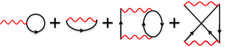
Figure 1: Feynman diagrams included in the GF2 self-energy. A black arrow line represents a Green’s function, while a red squiggle represents a two-electron integral. The first two diagrams are the frequency-independent Hartree and exchange terms, and are included in the Fock matrix. The next two diagrams are the frequency-dependent pair-bubble and second order exchange terms, and represent the second order correlation effects covered by $\mathbf{\Sigma}(\omega)$.

$$\mathbf{G}(\omega)=\bigr{[}(\mu+\omega)\mathbf{S}-\mathbf{F}-\mathbf{\Sigma}(\omega)\bigr{]}^{-1}~{}~{},$$ (2)

where $\mathbf{S}$ and $\mathbf{F}$ are the overlap and Fock matrices, $\mu$ is the chemical potential, $\omega$ is an imaginary frequency, and $\mathbf{\Sigma}(\omega)$ is the aforementioned frequency-dependent self-energy within the GF2 approximation containing second order diagrams from Fig. 1. We use a uniform grid of imaginary Matsubara frequencies $\omega_{n}=(2n+1)i\pi/\beta$, with a power mesh imaginary time gridAlbuquerque et al. (2007) running on the interval $0<\tau<\beta$, where $\beta$ is the inverse temperature. We choose to build the Green’s function on the frequency axis because of the simplicity of Eq. 2, in contrast to the expression for $\mathbf{G}(\tau)$ which is more cumbersome and requires integrations over $\tau$ pointsDahlen and van Leeuwen (2005). Once built, the imaginary frequency Green’s function can be fast Fourier transformed (FFT) to the imaginary time domain, $\mathbf{G}(\tau)$. The correlated density matrix $\mathbf{P}$ then is evaluated as

$$\mathbf{P}=-2\mathbf{G}({\scriptstyle\tau=\beta})~{}.$$ (3)

Provided with $\mathbf{P}$, the correlated Fock matrix is built by

$$F_{ij}=h_{ij}+\underset{kl}{\sum}P_{kl}(\textnormal{v}_{ijlk}-\frac{1}{2}\textnormal{v}_{iklj})~{},$$ (4)

where $h_{ij}$ and $\textnormal{v}_{ijlk}$ are one and two-electron integrals in the AO basis. Note that the (frequency-independent) first-order self-energy is already covered by the Hartree-Fock mean-field, $\Sigma_{\infty}={\sum_{kl}}P_{kl}(\textnormal{v}_{ijlk}-\frac{1}{2}\textnormal{v}_{iklj})$. Finally, the (frequency dependent) second order self energy can be built in the time-domain as

$$\begin{split}\Sigma_{ij}(\tau)=-\underset{klmnpq}{\sum}G_{kl}(\tau)G_{mn}(\tau)G_{pq}(-\tau)\\ \times\textnormal{v}_{imqk}\bigr{(}2\textnormal{v}_{lpnj}-\textnormal{v}_{nplj}\bigr{)}~{},\end{split}$$ (5)

and then FFT to the frequency domain. It is simpler to build $\mathbf{\Sigma}$ on the time axis, because in the $\tau$ domain the self-energy factorizes into simple products of Green’s functions, whereas in the $\omega$ domain it requires integrations of Green’s functions over frequencies. Furnished with an updated $\mathbf{F}$ and $\mathbf{\Sigma}(\omega)$, we can return to Eq. 2 and rebuild $\mathbf{G}(\omega)$. Taken altogether Eq. 2, 3, 4, and 5 present a self-consistent procedure for solving the Dyson equation in a second order approximation to the self energy. To initiate the self-consistency an approximate zeroth order Green’s function, $\mathbf{G}_{0}(\omega)$, is necessary, which practically can be supplied by DFT or Hartree-Fock (HF) calculations. In this work we use an initial HF Green’s function (i.e. $\mu\approx\frac{1}{2}(\epsilon_{\scriptscriptstyle HOMO}+\epsilon_{\scriptscriptstyle LUMO})$, $\mathbf{F}=\mathbf{F}_{\scriptstyle HF}$, and $\mathbf{\Sigma}(\omega)=\mathbf{0}$) generated via output from the Dalton electronic structure programAidas et al. (2013). At self-consistency $\mathbf{G}(\omega)$ will not depend on the starting-referenceKoval et al. (2014), though practically some initial guesses might be better than others for converging rapidly. As a final note, it should be understood that the Green’s function depends on $\mu$, and therefore $\mathbf{P}$ implicitly depends on $\mu$ as well. This means the chemical potential will need to be adjusted from iteration-to-iteration to maintain the correct electron number.

For purposes of comparison, we will also consider a non self-consistent Green’s function obtained from the first iteration of the Dyson equation, given by

$$\mathbf{G}_{1}(\omega)=\bigr{[}(\mu+\omega)\mathbf{S}-\mathbf{F}_{HF}-\mathbf{\Sigma}[G_{0}(\omega)]\bigr{]}^{-1}~{}~{}.$$ (6)

Here $\mathbf{\Sigma[G_{0}(\omega)]}$ is simply the self-energy obtained when $\mathbf{G}_{0}$, which in our case is $\mathbf{G}_{HF}$, is inserted into Eq. 5, and $\mu$ is set so that $\mathbf{G}_{0}(\omega)$ has good particle number. For conciseness, we will refer to this simply as G₀F2, in analogy to $G_{0}W_{0}$. Since this Green’s function is not self-consistent, it will carry a starting reference dependence.

Since the Green’s function obtained by self-consistent or non-self-consistent GF2 is expressed on an imaginary grid, we aim to employ the Extended Koopman’s Theorem (EKT)Smith and Day (1975); *EKT_Original_II; Pickup (1975); Matos and Day (1987); Morrison (1992); Morrison and Ayers (1995); Bozkaya (2013, 2014) to obtain ionization potentials and electron affinities, which are real axis quantities and can be used to produce the spectral density of states $A(\omega)$ expressed as $A(\omega)=-\frac{1}{\pi}\textnormal{Tr}[\textnormal{Im\,}\mathbf{G}(\omega)\mathbf{S}]$. We give a brief discussion of the EKT theory and implementation next.

III.1 Extended Koopmans’ Theorem

Given a system with Hamiltonian $\hat{H}$ and $N$ electron state $|{\scriptstyle N}\rangle$ satisfying $\hat{H}|{\scriptstyle N}\rangle=E|{\scriptstyle N}\rangle$, by using second-quantized operators, $\hat{a}|{\scriptstyle N}\rangle=|{\scriptstyle N-1}\rangle$, $\hat{a}^{\dagger}|{\scriptstyle N}\rangle=|{\scriptstyle N+1}\rangle$, the energies of the anion, neutral, and cation states can be expressed as

$$\begin{split}E_{{\scriptstyle N+1}}=\langle{\scriptstyle N}|\hat{a}\,\hat{H}\,\hat{a}^{\dagger}|{\scriptstyle N}\rangle~{},\\ E_{{\scriptstyle N}}=\langle{\scriptstyle N}|\hat{H}|{\scriptstyle N}\rangle~{},\\ E_{{\scriptstyle N-1}}=\langle{\scriptstyle N}|\hat{a}^{\dagger}\,\hat{H}\,\hat{a}|{\scriptstyle N}\rangle~{},\end{split}$$ (7)

respectively. It should be understoood these operators are expanded in a basis, $\hat{a}=\sum_{i}c_{i}\hat{\phi}_{i}$, with the expansion coefficients $c_{i}$ chosen so that the anion (cation) state remains normalizedMorrison and Ayers (1995). Provided with Eq. 7 the ionization potential ($I$) and electron affinity ($A$) can be defined as

$$\begin{split}I=E_{\scriptstyle N-1}-E_{\scriptstyle N}=-\langle{\scriptstyle N}|\hat{a}^{\dagger}[\hat{a},\hat{H}]|{\scriptstyle N}\rangle~{},\\ A=E_{\scriptstyle N}-E_{\scriptstyle N+1}=\langle{\scriptstyle N}|\hat{a}[\hat{a}^{\dagger},\hat{H}]|{\scriptstyle N}\rangle~{}.\end{split}$$ (8)

A Lagrangian for $I$ and $A$ can now be constructed, given by

$$\begin{split}\mathcal{L}_{I}=-\langle{\scriptstyle N}|\hat{a}^{\dagger}[\hat{a},\hat{H}]|{\scriptstyle N}\rangle+\epsilon(\langle{\scriptstyle N}|\hat{a}^{\dagger}\hat{a}|{\scriptstyle N}\rangle-1)~{},\\ \mathcal{L}_{A}=\langle{\scriptstyle N}|\hat{a}[\hat{a}^{\dagger},\hat{H}]|{\scriptstyle N}\rangle+\epsilon(\langle{\scriptstyle N}|\hat{a}\,\hat{a}^{\dagger}|{\scriptstyle N}\rangle-1)~{},\end{split}$$ (9)

where the right-hand term constrains the cation/anion state to be normalized. Expanding the operators in their basis, and exploiting that $\hat{a}\,\hat{a}^{\dagger}=\hat{1}-\hat{a}^{\dagger}\hat{a}$, the stationary solution $\delta\mathcal{L}/\delta{c_{i}^{\dagger}}=0$ of Eq. 9 yields the generalized eigenvalue problem

$$\begin{split}\mathbf{H}^{I}\mathbf{c}=\epsilon\mathbf{P}\mathbf{c}~{},\\ \mathbf{H}^{A}\mathbf{c}=\epsilon\mathbf{P}_{v}\mathbf{c}~{},\end{split}$$ (10)

where $[\mathbf{H}^{I}]_{ij}\equiv\langle{\scriptstyle N}|\hat{\phi}_{i}^{\dagger}[\hat{\phi}_{j},\hat{H}]|{\scriptstyle N}\rangle$ and $[\mathbf{H}^{A}]_{ij}\equiv-\langle{\scriptstyle N}|\hat{\phi}_{i}[\hat{\phi}^{\dagger}_{j},\hat{H}]|{\scriptstyle N}\rangle$ are generalized Fock matrices, and $[\mathbf{P}]_{ij}\equiv\langle{\scriptstyle N}|\hat{\phi}_{i}^{\dagger}\hat{\phi}_{j}|{\scriptstyle N}\rangle$ is the density matrix. $\mathbf{P}_{v}$ is the virtual (or “hole”) density matrix, which is defined within the orthogonal Löwdin basis as $\mathbf{P}_{v}\equiv 2\mathbf{I}-\mathbf{P}$, where $\mathbf{I}$ is the identity matrix and the factor of two accounts for double occupation in our spin-restricted formalism, or equivalently in terms of Green’s functions in the Löwdin basis as $\mathbf{P}_{v}=-2\mathbf{G}({\scriptstyle\tau=0_{+}})$.

For practical calculations we want to connect Eq. 10 to Green’s function many-body theory in the following way: From the definition of the time-dependent single-particle Green’s functionFetter and Walecka (2003), $G(\tau)$, one can show

$$\begin{split}\lim_{\tau\rightarrow 0}\dfrac{\partial G(\tau)}{\partial\tau}=\Biggr{\{}\begin{matrix}\langle N|\hat{a}[\hat{a}^{\dagger},\hat{H}]|N\rangle~{},&\tau>0\\ \langle N|\hat{a}^{\dagger}[\hat{a},\hat{H}]|N\rangle~{},&\tau<0\end{matrix}\end{split}$$ (11)

For compactness we simply write these two possibilities as $\partial_{\tau}G(\tau)|_{0^{+}}$ and $\partial_{\tau}G(\tau)|_{0^{-}}$. Eq. 11 has this form because of the discontinuity in the Green’s function at $\tau=0$, and furthermore $G(\tau)=-G(\tau+\beta)$, which means that $\partial_{\tau}G(\tau)|_{0^{-}}=-\partial_{\tau}G(\tau)|_{\beta}$. The important point of Eq. 11 is the generalized Fockians appearing in the standard EKT Eq. 10 can be replaced with time-derivatives of the Green’s function on the imaginary-domain in the AO basis. Introducing a matrix representation for the Green’s function in this basis, $\mathbf{G}(\tau)$, performing the transformation $\mathbf{c}=\mathbf{P}^{-1/2}\mathbf{c}^{\prime}$ (or $\mathbf{c}=\mathbf{P}_{v}^{-1/2}\mathbf{c}^{\prime}$) and multiplying on the left with $\mathbf{P}^{-1/2}$ (or $\mathbf{P}^{-1/2}_{v}$) results in

$$\begin{split}\Delta_{-}\mathbf{c}^{\prime}=\epsilon_{I}\mathbf{c}^{\prime}~{},~{}\epsilon_{I}=I+\mu\\ \Delta_{+}\mathbf{c}^{\prime}=\epsilon_{A}\mathbf{c}^{\prime}~{},~{}\epsilon_{A}=A+\mu\\ \Delta_{-}=2\mathbf{P}^{-1/2}\partial_{\tau}\mathbf{G}(\tau)|_{0^{-}}\mathbf{P}^{-1/2}\\ \Delta_{+}=-2\mathbf{P}^{-1/2}_{v}\partial_{\tau}\mathbf{G}(\tau)|_{0^{+}}\mathbf{P}^{-1/2}_{v}\end{split}$$ (12)

where $\mathbf{P}=-2\mathbf{G}({\scriptstyle\tau=\beta})$, and $\mathbf{P}_{v}=-2\mathbf{G}({\scriptstyle\tau=0_{+}})$. The factor of two in Eq. 12 accounts for double occupation in our spin-restricted formalism. We emphasize Eq. 12 assumes that $\mathbf{G}(\tau)$ and $\mathbf{P}$ have been pre-transformed to the Löwdin basis. Eq. 12 shows that diagonalization of the $\Delta_{-}$ and $\Delta_{+}$ matrices gives eigenvalues which, after subtracting out the chemical potential $\mu$, yield the ionization potentials and electron affinities respectively. For example, if the Hartree-Fock Green’s functions were inserted in Eq. 12 then this would yield simply the Koopman’s theorem IPs and EAs (in fact this is a good way to check the accuracy of one’s grid). Conceptually, the form of Eq. 12 can be understood by realizing that $\mathbf{G}(\tau)$ for $\tau$ near $\beta$ describes the particle distribution of the system and consequently electron removal, whereas for $\tau$ near $0_{+}$ it contains information on the hole distribution and therefore electron attachment.

One subtlety is that diagonalizing $\Delta_{\pm}$ will of course yield as many eigenvalues as there are AO basis functions, $N_{b}$, yet only some of these eigenvalues may be physically meaningful as IPs or EAs. We find the simplest way to identify the correct eigenvalues is by the corresponding Dyson occupations

$$\begin{split}\mathbf{C}_{-}^{\dagger}\mathbf{P}\,\mathbf{C}_{-}=\mathbf{D}~{}~{},\\ \mathbf{C}_{+}^{\dagger}\mathbf{P}_{v}\mathbf{C}_{+}=\mathbf{D}_{v}~{}~{}.\end{split}$$ (13)

Here $\mathbf{C}_{\pm}$ is the matrix of eigenvectors, $\mathbf{C}=\{\mathbf{c}^{{}^{\prime}}_{1},\mathbf{c}^{{}^{\prime}}_{2},\ldots\}$, obtained from diagonalizing $\Delta_{\pm}$. The diagonal elements of $\mathbf{D}$ ($\mathbf{D}_{v}$) correspond to occupations of Dyson orbitals for electron removal (attachment). As a consistency check one should find that $\textnormal{Tr}[\mathbf{D}]=N$, and $\textnormal{Tr}[\mathbf{D}_{v}]=2N_{b}-N$. Essentially the orbitals with large occupations (roughly speaking $1<[\mathbf{D}]_{ii}<2$) will indicate the IPs/EAs one is interested in.

As a final note, we stress again that the use of the Extended Koopmans’ Theorem is not limited to GF2 or even Green’s function methods, and has been employed with a variety of methods at different levels of theory in the pastSmith and Day (1975); *EKT_Original_II; Pickup (1975); Morrison (1992); Morrison and Liu (1992); Cioslowski et al. (1997); Pernal and Cioslowski (2005); Dahlen and van Leeuwen (2005); Stan et al. (2009); Bozkaya (2013). It has been a matter of debate whether or not the lowest IP given using EKT is exact, or whether or not higher IPs obtained from this method are physically meaningfulErnzerhof (2009); Cioslowski et al. (1997). We do not investigate this in this paper, but rather, show that EKT offers reasonable values for IPs and EAs. Presumably, if one were to use a more accurate Green’s function, one would obtain more accurate IPs and EAs.

IV Computational Details

Our GF2 and G₁F2 calculations were carried out on an imaginary grid with 20,000 frequency points and 4,400 time pointsAlbuquerque et al. (2007), with an inverse-temperature of $\beta$= 100.0 [$a.u^{-1}$]. Experimentally determined geometries were used for the moleculesJohnson (2011). The basis sets used were Dunning’s aug-cc-pVXZ seriesDunning (1989); Woon and Dunning (1993). Restricted Hartree-Fock calculations carried out in the Dalton programAidas et al. (2013) were used to generate an initial Green’s function $\mathbf{G}_{0}(\omega)$ as input for our GF2 procedure. All GF2 and G₁F2 calculations reported here are all-electron. The Hartree Fock IPs and EAs were obtained from standard Koopmans’ Theorem as the negative of the HOMO and LUMO eigenvalues, respectively. To obtain accurate reference theoretical values, IPs and EAs were computed from energy differences of the charged and neutral species, using all-electron unrestricted UCCSD(T) calculations with the Gaussian 09 package Frisch et al. (2009) (“UCCSD(T)=Full” keyword). Let us stress that since IP and EA values in UCCSD(T) are calculated as a difference between the charged and neutral species, the obtained values not only include the benefit of energy lowering due to the use of an unrestricted method but also can take advantage of error cancellations. This stands in stark contrast to the IPs and EAs calculated from GF2 that is based on a restricted reference (RHF) and does not benefit from error cancellation due to calculating differences.

V Results

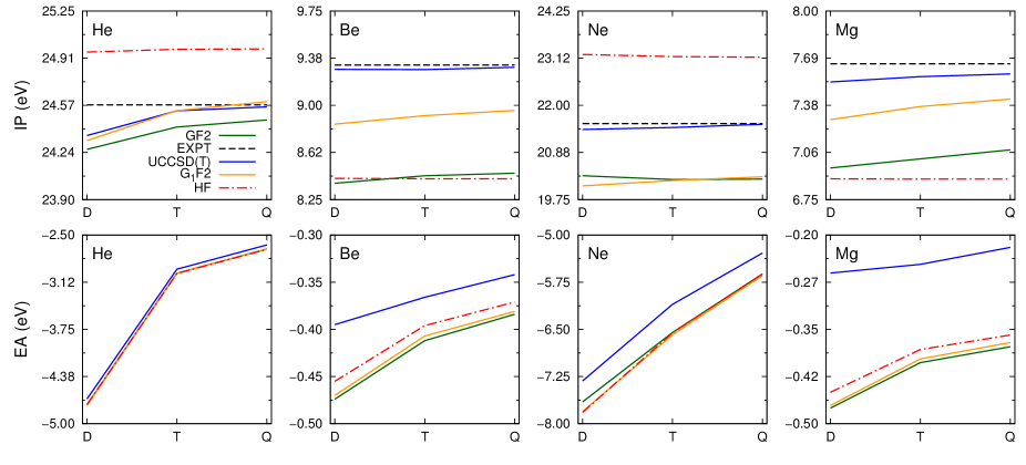
Figure 2: Ionization potentials and electron affinities of atoms calculated with the aug-cc-pVXZ basis set.

	GF2	G1F2	HF	UCCSD(T)	Expt
Be2	6.21	6.99	6.62	7.42
BH3	12.82	13.13	13.52	13.17
C2H2	10.24	11.24	11.19	11.36	11.41
C2H4	9.54	10.22	10.21	10.55	10.51
CO	12.20	14.46	15.09	13.80	14.01
CO2	11.71	12.88	14.82	13.61	13.78
H2CO	9.12	9.74	12.02	10.74	10.88
H2O	11.31	11.47	13.86	12.54	12.65
H2O2	9.51	10.32	13.31	11.46	11.70
HCN	12.26	13.49	13.50	13.62	13.61
HF	14.68	14.66	17.68	16.02	16.06
Li2	4.69	5.28	4.95	5.23
LiF	9.89	9.70	12.91	11.37
LiH	7.77	7.91	8.20	7.94	7.90
MgH2	9.80	9.93	10.09	9.76
N2	13.53	14.97	17.26	15.36	15.58
Na2	4.67	4.80	4.51	4.85
NaF	8.38	8.15	11.59	9.98
NaH	6.82	7.08	7.43	7.04
NaLi	4.69	4.96	4.71	5.01
NaOH	6.42	6.35	9.11	7.86
NH3	9.86	10.10	11.67	10.76	10.82

Table 1: Calculated ionization potentials in eV using self-consistent GF2 and non self-consistent G₁F2. Shown for comparison are the ionization potentials from Hartree-Fock Koopmans’ Theorem and UCCSD(T) energy-differences, along with experimental values. All calculations use aug-cc-pVDZ.

Our ability to obtain accurate IPs and EAs will be affected by the intrinsic accuracy of EKT, the performance of GF2, and the choice of basis set. We will not discuss the accuracy of EKT in this work, but will instead focus on the latter two points. To assess the performance of GF2 and G₁F2, we have carried out a series of calculations on several closed shell atoms and molecules. We start from atomic calculations since they are simpler, and then turn our discussion to small molecules. We have carried out UCCSD(T) calculations on each system to be used as a reference point throughout our discussion. We note that for the closed shell atoms and many of the molecules studied here the EA will be negative, meaning the system does not bind an extra electron, and in the complete basis set limit the EA would approach zero. However we include these systems in our analysis as a proof of concept, because we find the EA from GF2 with EKT for most cases agrees reasonably well with the results from UCCSD(T) energy differences, as well as from HF Koopmans’ Theorem.

V.1 Atoms

In Figure 2, we present for a series of closed-shell atoms the IPs and EAs calculated with GF2 and G₁F2 using EKT, with HF using standard Koopmans’ Theorem, and with UCCSD(T) using energy differences, compared against experimental values when available. Figure 2 illustrates that the IPs obtained from GF2 for these atoms are well converged with the basis set and systematically underestimate experimental and UCCSD(T) IPs. In comparison with experimental values, the IPs can differ by up to 1 eV. For these atoms the best agreement occurs in the case of He, with a difference from experiment of around 0.1 eV. For comparison, calculations were carried out non self-consistently (G₁F2), and it was found that these values were in closer agreement with both UCCSD(T) and experimental IPs than the self-consistent GF2 IPs. This effect was observed previously in the work of Dahlen and van LeeuwenDahlen and van Leeuwen (2005); Stan et al. (2009). In contrast, self-consistency appears to have a small effect on the EAs of these systems. The largest difference in electron affinity occurs for Ne, with a difference of 0.2 eV. The majority of the atoms have a difference on the order of 1 meV between self-consistent and non self-consistent calculations. It should be noted that the EAs are not converged with respect to the basis set. Between basis sets the EAs can vary by around 1 eV, in a similar fashion to the UCCSD(T) electron affinities.

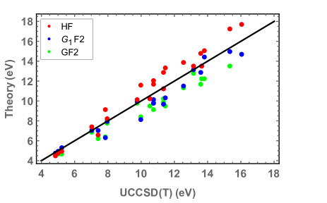
Figure 3: HF, G₁F2, and GF2 IPs for molecules compared against reference UCCSD(T) values, calculated with aug-cc-pVDZ.

V.2 Molecules

Turning now to the molecules, in Tables 1 and 2 we present our calculated IPs and EAs. Focusing first on the IPs, similar to the atoms, we find that GF2 tends to systematically underestimate experimental values. Furthermore, comparing against UCCSD(T) reference values in Fig. 3 we find that GF2 systematically underestimates UCCSD(T) as well. In contrast, non-self-consistent G₁F2 again yields overall slightly larger IPs that are in better agreement with UCCSD(T) and experimental values than self-consistent GF2. This same effect has been observed in the work of Rostgaard, Jacobsen, and ThygesenRostgaard et al. (2010) with self-consistent GW and non-self-consistent G₀W₀ applied to a similar set of molecular systems, where it was interpreted as being caused by overscreening in the former case and underscreening in the latter. GF2 does not have a series of bubble diagrams that are commonly thought to be responsible for the screening effects. However, the self-consistent GF2 has a series of composite type diagrams resulting from the iterative procedure where four of the diagrams from Figure 1 are joined together into series of ladder like diagrams. These diagrams most likely have effects similar to the series of bubbles in self-consistent GW which are causing overscreening. We believe that since the self-consistent GF2 redefines the Fock matrix during iterations, the results of the iterative procedure are less likely to overestimate the amount of correlation as in the case of MP2. Therefore, we assume that the good agreement of G₁F2 with UCCSD(T) is fortuitous. One could speculate that in iterative GF2 introducing the third order diagrams may be much more beneficial and would lead to systematically convergent IP results.

o

Examining the EAs now, we find GF2 tends to give results which are slightly lower than both HF and UCCSD(T) values. For a few of the molecules with positive EAs, GF2 and G₁F2 do not recover the proper sign. However we emphasize that the EA is a notoriously difficult property to calculate, and from comparing our results to those from EKT-MPn in Table 2 of Ref. Bozkaya (2014) it is not uncommon for a method to occasionally predict the incorrect sign for even small closed-shell molecules. Interestingly, whether or not the calculations are carried out self-consistently does not appear to have such a drastic effect on the EAs, as the GF2, G₁F2, and HF EAs tend to be quite similar to the UCCSD(T) values for many of the molecules. We think the simplest explanation for this is the following: in the imaginary time Green’s function EKT approach we are using, the EAs are essentially determined by the “hole”-part of $\mathbf{G}(\tau)$ near $\tau=0_{+}$, and the IPs likewise by the “particle”-part near $\tau=\beta$. Because these systems are small and weakly correlated, it may be that the “hole” or virtual orbital space does not relax as much between HF, G₁F2, and GF2, as does the “particle” or occupied orbital space. Regardless, we find it encouraging that EAs can systematically be recovered from simply the imaginary time Green’s function of the neutral system, without need for considering molecular anions.

	GF2	G1F2	HF	UCCSD(T)
Be2	-0.30	-0.28	-0.21	0.34
BH3	-0.92	-0.94	-0.88	-0.15
C2H2	-1.02	-1.02	-1.02	-0.99
C2H4	-1.09	-1.10	-1.10	-1.22
CO	-2.34	-2.33	-2.15	-1.81
CO2	-1.46	-1.47	-1.49	-2.23
H2CO	-0.94	-0.90	-0.90	-1.19
H2O	-0.93	-0.96	-0.96	-0.75
H2O2	-1.05	-1.08	-1.08	-1.16
HCN	-0.83	-0.79	-0.79	-0.69
HF	-0.95	-0.97	-0.97	-0.80
Li2	-0.10	-0.10	-0.08	0.32
LiF	0.27	0.29	0.29	0.34
LiH	0.20	0.20	0.21	0.30
MgH2	-0.45	-0.44	-0.44	-0.50
N2	-2.81	-4.02	-3.39	-2.60
Na2	-0.05	-0.05	-0.01	0.36
NaF	0.43	0.43	0.44	0.48
NaH	0.22	0.23	0.24	0.32
NaLi	-0.07	-0.07	-0.04	0.35
NaOH	0.32	0.31	0.31	0.39
NH3	-0.94	-0.97	-0.98	-0.75

Table 2: Calculated electron affinities in eV using self-consistent GF2 and non self-consistent G₁F2. Shown for comparison are the electron affinities from Hartree-Fock Koopmans’ Theorem, and UCCSD(T) energy-differences. All calculations use aug-cc-pVDZ.

VI Conclusions

In this work we have investigated how reliably IPs and EAs can be calculated from the Extended Koopmans’ Theorem (EKT) with an imaginary time Green’s function in a second order approximation (GF2). In contrast to prior EKT works that determined the EA indirectly as the IP of the anionBozkaya (2014), in this work we calculated both IPs and EAs directly from the imaginary time Green’s function of the neutral system alone. Overall, we find that self-consistent GF2 with EKT recovers IPs and EAs that are systematically smaller than UCCSD(T) energy-differences and experiment reference values. Interestingly, non-self-consistent G₁F2 on a Hartree-Fock reference consistently gives slightly larger IPs and EAs than self-consistent GF2, similar to what has been found with GW and G₀W₀ for IPsRostgaard et al. (2010). Because GF2 is defined in terms of the bare Coulomb interaction rather than the screened interaction as in GW, this suggests that the cause of the systematic underestimation of quasiparticle spectra by self-consistent vs non-self-consistent Green’s function methods may be more general than being specifically the result of over or underscreening caused by a series of bubble diagrams present in the the GW approach.

Regardless of the particular performance of GF2 or G₁F2, the more general point of this work is that the EKT in conjunction with self-consistent Green’s function theory offers a reliable procedure for the unbiased theoretical determination of quasiparticle spectra. Essentially the underlying scheme in this Green’s function EKT approach is that the IPs are determined by the eigenvalues of the time-derivative of the “particle”-part of $\mathbf{G}(\tau)$ at $\tau=\beta$, while the EAs are likewise found from the “hole”-part of $\mathbf{G}(\tau)$ at $\tau=0_{+}$. In this way the full quasiparticle spectra can in principle be reconstructed from simply the Green’s function on the imaginary time domain, without the need for analytic continuationGunnarsson et al. (2010); Jarrell and Gubernatis (1996); Gubernatis et al. (1991) or other numerical methods. Therefore the EKT allows one to obtain real axis quasiparticle spectra while still enjoying the computational benefits of using an imaginary axis Green’s function implementation. Furthermore, the advantages of the EKT are that it is simple, is applicable to a Green’s function from any level of theory, requires only a trivial amount of computational time, and can be implemented in a blackbox manner.

VII Acknowledgments

D. Zgid, A. Welden and J.J. Phillips acknowledge support from a DOE grant no. ER16391 and an XSEDE allocation allowing us to use the STAMPEDE supercomputer.

References

- Hohenberg and Kohn (1964) Hohenberg, P.; Kohn, W. Phys. Rev. 1964, 136, B864–B871.
- Kohn and Sham (1965) Kohn, W.; Sham, L. J. Phys. Rev. 1965, 140, A1133–A1138.
- Parr and Yang (1989) Parr, R. G.; Yang, W. Density-Functional Theory of Atoms and Molecules; Oxford University Press: New York, 1989.
- Coester and Kümmel (1960) Coester, F.; Kümmel, H. Nuclear Physics 1960, 17, 477 – 485.
- Cizek (1991) Cizek, J. Theoretica chimica acta 1991, 80, 91–94.
- Bartlett and Musiał (2007) Bartlett, R. J.; Musiał, M. Rev. Mod. Phys. 2007, 79, 291–352.
- Scuseria (1999) Scuseria, G. E. J. Phys. Chem. A 1999, 103, 4782–4790.
- Burke (2012) Burke, K. J. Chem. Phys. 2012, 136, –.
- Bredow and Gerson (2000) Bredow, T.; Gerson, A. R. Phys. Rev. B 2000, 61, 5194–5201.
- de P. R. Moreira et al. (2002) de P. R. Moreira, I.; Illas, F.; Martin, R. L. Phys. Rev. B 2002, 65, 155102.
- Perdew and Levy (1983) Perdew, J. P.; Levy, M. Phys. Rev. Lett. 1983, 51, 1884–1887.
- Perdew (1985) Perdew, J. P. Int. J. Quantum Chem. 1985, 28, 497–523.
- Stoudenmire et al. (2012) Stoudenmire, E. M.; Wagner, L. O.; White, S. R.; Burke, K. Phys. Rev. Lett. 2012, 109, 056402.
- Baerends et al. (2013) Baerends, E. J.; Gritsenko, O. V.; van Meer, R. Phys. Chem. Chem. Phys. 2013, 15, 16408–16425.
- Foerster et al. (2011) Foerster, D.; Koval, P.; Sánchez-Portal, D. J. Chem. Phys. 2011, 135, –.
- Caruso et al. (2013) Caruso, F.; Rinke, P.; Ren, X.; Rubio, A.; Scheffler, M. Phys. Rev. B 2013, 88, 075105.
- Phillips and Zgid (2014) Phillips, J. J.; Zgid, D. J. Chem. Phys. 2014, 140, –.
- Koval et al. (2014) Koval, P.; Foerster, D.; Sánchez-Portal, D. Phys. Rev. B 2014, 89, 155417.
- Dahlen and van Leeuwen (2005) Dahlen, N. E.; van Leeuwen, R. J. Chem. Phys. 2005, 122, –.
- Stan et al. (2009) Stan, A.; Dahlen, N. E.; van Leeuwen, R. J. Chem. Phys. 2009, 130, –.
- Møller and Plesset (1934) Møller, C.; Plesset, M. S. Phys. Rev. 1934, 46, 618–622.
- Hedin (1965) Hedin, L. Phys. Rev. 1965, 139, A796–A823.
- Albertsen and Jørgensen (1979) Albertsen, P.; Jørgensen, P. J. Chem. Phys. 1979, 70, 3254–3263.
- B. and Öhrn (1981) B., J. O.; Öhrn, Y. Chem. Phys. Lett. 1981, 77, 548 – 554.
- Schirmer et al. (1983) Schirmer, J.; Cederbaum, L. S.; Walter, O. Phys. Rev. A 1983, 28, 1237–1259.
- Cederbaum (1990) Cederbaum, L. S. Int. J. Quantum Chem. 1990, 38, 393–404.
- Massidda et al. (1995) Massidda, S.; Continenza, A.; Posternak, M.; Baldereschi, A. Phys. Rev. Lett. 1995, 74, 2323–2326.
- Massidda et al. (1997) Massidda, S.; Continenza, A.; Posternak, M.; Baldereschi, A. Phys. Rev. B 1997, 55, 13494–13502.
- Ku and Eguiluz (2002) Ku, W.; Eguiluz, A. G. Phys. Rev. Lett. 2002, 89, 126401.
- Rostgaard et al. (2010) Rostgaard, C.; Jacobsen, K. W.; Thygesen, K. S. Phys. Rev. B 2010, 81, 085103.
- Ortiz (2013) Ortiz, J. V. Wiley Interdisciplinary Reviews: Computational Molecular Science 2013, 3, 123–142.
- Gunnarsson et al. (2010) Gunnarsson, O.; Haverkort, M. W.; Sangiovanni, G. Phys. Rev. B 2010, 82, 165125.
- Jarrell and Gubernatis (1996) Jarrell, M.; Gubernatis, J. E. Physics Reports 1996, 269, 133–195.
- Gubernatis et al. (1991) Gubernatis, J.; Jarrell, M.; Silver, R.; Sivia, D. Physical Review B 1991, 44, 6011.
- Smith and Day (1975) Smith, D. W.; Day, O. W. The Journal of Chemical Physics 1975, 62, 113–114.
- Day et al. (1975) Day, O. W.; Smith, D. W.; Morrison, R. C. The Journal of Chemical Physics 1975, 62, 115–119.
- Pickup (1975) Pickup, B. T. Chem. Phys. Lett. 1975, 33, 422 – 426.
- Katriel and Davidson (1980) Katriel, J.; Davidson, E. R. Proceedings of the National Academy of Sciences 1980, 77, 4403–4406.
- Matos and Day (1987) Matos, J. M. O.; Day, O. W. International Journal of Quantum Chemistry 1987, 31, 871–892.
- Morrison (1992) Morrison, R. C. J. Chem. Phys. 1992, 96, 3718–3722.
- Sundholm and Olsen (1993) Sundholm, D.; Olsen, J. The Journal of Chemical Physics 1993, 98, 3999–4002.
- Morrison and Ayers (1995) Morrison, R. C.; Ayers, P. W. J. Chem. Phys. 1995, 103, 6556–6561.
- Cioslowski et al. (1997) Cioslowski, J.; Piskorz, P.; Liu, G. The Journal of Chemical Physics 1997, 107, 6804–6811.
- Olsen and Sundholm (1998) Olsen, J.; Sundholm, D. cpl 1998, 288, 282 – 288.
- Pernal and Cioslowski (2001) Pernal, K.; Cioslowski, J. J. Chem. Phys. 2001, 114, 4359–4361.
- Ernzerhof (2009) Ernzerhof, M. J. Chem. Theory Comput. 2009, 5, 793–797.
- Bozkaya (2013) Bozkaya, U. The Journal of Chemical Physics 2013, 139, –.
- Bozkaya (2014) Bozkaya, U. Journal of Chemical Theory and Computation 2014, 10, 2041–2048.
- Reed et al. (1985) Reed, A. E.; Weinstock, R. B.; Weinhold, F. J. Chem. Phys. 1985, 83, 735.
- Morrison and Liu (1992) Morrison, R. C.; Liu, G. J. Comp. Chem. 1992, 13, 1004–1010.
- Pernal and Cioslowski (2005) Pernal, K.; Cioslowski, J. Chem. Phys. Lett. 2005, 412, 71 – 75.
- Sasaki and Yoshimine (1974) Sasaki, F.; Yoshimine, M. Phys. Rev. A 1974, 9, 17–25.
- Sasaki and Yoshimine (1974) Sasaki, F.; Yoshimine, M. Phys. Rev. A 1974, 9, 26–34.
- Feller and Davidson (1989) Feller, D.; Davidson, E. R. J. Chem. Phys. 1989, 90, 1024–1030.
- Kendall et al. (1992) Kendall, R. A.; Dunning, T. H.; Harrison, R. J. J. Chem. Phys. 1992, 96, 6796–6806.
- Rösch and Trickey (1997) Rösch, N.; Trickey, S. B. J. Chem. Phys. 1997, 106, 8940–8941.
- Galbraith and Schaefer (1996) Galbraith, J. M.; Schaefer, H. F. J. Chem. Phys. 1996, 105, 862–864.
- Jensen (2010) Jensen, F. J. Chem. Theory Comput. 2010, 6, 2726–2735.
- Emrich (1981) Emrich, K. Nuclear Physics A 1981, 351, 379 – 396.
- Sekino and Bartlett (1984) Sekino, H.; Bartlett, R. J. International Journal of Quantum Chemistry 1984, 26, 255–265.
- Geertsen et al. (1989) Geertsen, J.; Rittby, M.; Bartlett, R. J. Chem. Phys. Lett. 1989, 164, 57 – 62.
- Stanton and Bartlett (1993) Stanton, J. F.; Bartlett, R. J. J. Chem. Phys. 1993, 98, 7029–7039.
- Krylov (2008) Krylov, A. I. Annual Review of Physical Chemistry 2008, 59, 433–462.
- Nooijen and Bartlett (1995) Nooijen, M.; Bartlett, R. J. J. Chem. Phys. 1995, 102, 3629–3647.
- Nooijen and Bartlett (1997) Nooijen, M.; Bartlett, R. J. J. Chem. Phys. 1997, 106, 6449–6455.
- Musial et al. (2003) Musial, M.; Kucharski, S. A.; Bartlett, R. J. The Journal of Chemical Physics 2003, 118, 1128–1136.
- Musial and Bartlett (2003) Musial, M.; Bartlett, R. J. J. Chem. Phys. 2003, 119, 1901–1908.
- Musial and Bartlett (2004) Musial, M.; Bartlett, R. J. Chem. Phys. Lett. 2004, 384, 210 – 214.
- Kamiya and Hirata (2007) Kamiya, M.; Hirata, S. J. Chem. Phys. 2007, 126, –.
- Musial and Bartlett (2007) Musial, M.; Bartlett, R. J. J. Chem. Phys. 2007, 127, –.
- Nooijen and Snijders (1992) Nooijen, M.; Snijders, J. G. Int. J. Quantum Chem. 1992, 44, 55–83.
- Nooijen and Snijders (1993) Nooijen, M.; Snijders, J. G. Int. J. Quantum Chem. 1993, 48, 15–48.
- Nooijen and Snijders (1995) Nooijen, M.; Snijders, J. G. The Journal of Chemical Physics 1995, 102, 1681–1688.
- Schirmer (1982) Schirmer, J. Phys. Rev. A 1982, 26, 2395–2416.
- Tarantelli and Cederbaum (1989) Tarantelli, A.; Cederbaum, L. S. Phys. Rev. A 1989, 39, 1656–1664.
- Flores-Moreno et al. (2010) Flores-Moreno, R.; Melin, J.; Dolgounitcheva, O.; Zakrzewski, V. G.; Ortiz, J. V. Int. J. Quantum Chem. 2010, 110, 706–715.
- Cederbaum (1973) Cederbaum, L. Theoretica chimica acta 1973, 31, 239–260.
- Ortiz (1988) Ortiz, J. V. J. Chem. Phys. 1988, 89, 6348–6352.
- Ortiz (1989) Ortiz, J. V. Int. J. Quantum Chem. 1989, 36, 321–332.
- Ortiz (1996) Ortiz, J. V. The Journal of Chemical Physics 1996, 104, 7599–7605.
- Ortiz (1998) Ortiz, J. V. The Journal of Chemical Physics 1998, 108, 1008–1014.
- Deleuze et al. (1999) Deleuze, M. S.; Giuffreda, M. G.; Fran√ßois, J.-P.; Cederbaum, L. S. J. Chem. Phys. 1999, 111, 5851–5865.
- Seabra et al. (2004) Seabra, G. M.; Kaplan, I. G.; Zakrzewski, V. G.; Ortiz, J. V. The Journal of Chemical Physics 2004, 121, 4143–4155.
- Trofimov and Schirmer (2005) Trofimov, A. B.; Schirmer, J. The Journal of Chemical Physics 2005, 123, –.
- Starcke et al. (2006) Starcke, J. H.; Wormit, M.; Schirmer, J.; Dreuw, A. Chem. Phys. 2006, 329, 39 – 49, Electron Correlation and Multimode Dynamics in Molecules (in honour of Lorenz S. Cederbaum).
- Müller and Cederbaum (2006) Müller, I. B.; Cederbaum, L. S. J. Chem. Phys. 2006, 125, –.
- Godby et al. (1986) Godby, R. W.; Schlüter, M.; Sham, L. J. Phys. Rev. Lett. 1986, 56, 2415–2418.
- Grüning et al. (2006) Grüning, M.; Marini, A.; Rubio, A. J. Chem. Phys. 2006, 124, –.
- Perdew and Zunger (1981) Perdew, J. P.; Zunger, A. Phys. Rev. B 1981, 23, 5048–5079.
- Perdew et al. (1982) Perdew, J. P.; Parr, R. G.; Levy, M.; Balduz Jr., J. L. Phys. Rev. Lett. 1982, 49, 1691.
- Ruzsinszky et al. (2006) Ruzsinszky, A.; Perdew, J. P.; Csonka, G. I.; Vydrov, O. A.; Scuseria, G. E. J. Chem. Phys. 2006, 125, 194112.
- Sànchez et al. (2006) Sànchez, P. M.; Cohen, A. J.; Yang, W. J. Chem. Phys. 2006, 125, 201102.
- Cohen et al. (2008) Cohen, A. J.; Mori-Sánchez, P.; Yang, W. Phys. Rev. B 2008, 77, 115123.
- Moussa et al. (2012) Moussa, J. E.; Schultz, P. A.; Chelikowsky, J. R. J. Chem. Phys. 2012, 136, –.
- Seidl et al. (1996) Seidl, A.; Görling, A.; Vogl, P.; Majewski, J. A.; Levy, M. Phys. Rev. B 1996, 53, 3764–3774.
- Heyd et al. (2003) Heyd, J.; Scuseria, G.; Ernzerhof, M. J. Chem. Phys. 2003, 118, 8207–8215.
- Heyd and Scuseria (2004) Heyd, J.; Scuseria, G. J. Chem. Phys. 2004, 120, 7274–7280.
- Heyd et al. (2005) Heyd, J.; Peralta, J. E.; Scuseria, G. E.; Martin, R. L. J. Chem. Phys. 2005, 123, –.
- Brothers et al. (2008) Brothers, E. N.; Izmaylov, A. F.; Normand, J. O.; Barone, V.; Scuseria, G. E. J. Chem. Phys. 2008, 129, –.
- Henderson et al. (2011) Henderson, T. M.; Paier, J.; Scuseria, G. E. physica status solidi b 2011, 248, 767–774.
- Hybertsen and Louie (1986) Hybertsen, M. S.; Louie, S. G. Phys. Rev. B 1986, 34, 5390–5413.
- Onida et al. (2002) Onida, G.; Reining, L.; Rubio, A. Rev. Mod. Phys. 2002, 74, 601–659.
- Fuchs et al. (2007) Fuchs, F.; Furthmüller, J.; Bechstedt, F.; Shishkin, M.; Kresse, G. Phys. Rev. B 2007, 76, 115109.
- Blase et al. (2011) Blase, X.; Attaccalite, C.; Olevano, V. Phys. Rev. B 2011, 83, 115103.
- Marom et al. (2011) Marom, N.; Moussa, J. E.; Ren, X.; Tkatchenko, A.; Chelikowsky, J. R. Phys. Rev. B 2011, 84, 245115.
- Marom et al. (2011) Marom, N.; Ren, X.; Moussa, J. E.; Chelikowsky, J. R.; Kronik, L. Phys. Rev. B 2011, 84, 195143.
- Liao and Carter (2011) Liao, P.; Carter, E. A. Phys. Chem. Chem. Phys. 2011, 13, 15189–15199.
- Toroker et al. (2011) Toroker, M. C.; Kanan, D. K.; Alidoust, N.; Isseroff, L. Y.; Liao, P.; Carter, E. A. Phys. Chem. Chem. Phys. 2011, 13, 16644–16654.
- Isseroff and Carter (2012) Isseroff, L. Y.; Carter, E. A. Phys. Rev. B 2012, 85, 235142.
- Marom et al. (2012) Marom, N.; Caruso, F.; Ren, X.; Hofmann, O. T.; Körzdörfer, T.; Chelikowsky, J. R.; Rubio, A.; Scheffler, M.; Rinke, P. Phys. Rev. B 2012, 86, 245127.
- Körzdörfer and Marom (2012) Körzdörfer, T.; Marom, N. Phys. Rev. B 2012, 86, 041110.
- Bruneval and Marques (2013) Bruneval, F.; Marques, M. A. L. J. Chem. Theory Comput. 2013, 9, 324–329.
- Perdew et al. (1996) Perdew, J. P.; Burke, K.; Ernzerhof, M. Phys. Rev. Lett. 1996, 77, 3865–3868.
- Ernzerhof and Scuseria (1999) Ernzerhof, M.; Scuseria, G. E. J. Chem. Phys. 1999, 110, 5029–5036.
- Adamo and Barone (1999) Adamo, C.; Barone, V. J. Chem. Phys. 1999, 110, 6158–6170.
- Holm and von Barth (1998) Holm, B.; von Barth, U. Phys. Rev. B 1998, 57, 2108–2117.
- Schöne and Eguiluz (1998) Schöne, W.-D.; Eguiluz, A. G. Phys. Rev. Lett. 1998, 81, 1662–1665.
- Faber et al. (2011) Faber, C.; Attaccalite, C.; Olevano, V.; Runge, E.; Blase, X. Phys. Rev. B 2011, 83, 115123.
- Strange et al. (2011) Strange, M.; Rostgaard, C.; Häkkinen, H.; Thygesen, K. S. Phys. Rev. B 2011, 83, 115108.
- Caruso et al. (2012) Caruso, F.; Rinke, P.; Ren, X.; Scheffler, M.; Rubio, A. Phys. Rev. B 2012, 86, 081102.
- Mattuck (1976) Mattuck, R. A Guide to Feynman Diagrams in the Many-body Problem; Dover Books on Physics Series; Dover Publications, Incorporated, 1976.
- Fetter and Walecka (2003) Fetter, A.; Walecka, J. Quantum Theory of Many-particle Systems; Dover Books on Physics; Dover Publications, 2003; p 65.
- Albuquerque et al. (2007) Albuquerque, A. et al. J. Magn. Magn. Mater. 2007, 310, 1187 – 1193, Proceedings of the 17th International Conference on Magnetism The International Conference on Magnetism.
- Aidas et al. (2013) Aidas, K. et al. Wiley Interdisciplinary Reviews: Computational Molecular Science 2013, n/a–n/a.
- Johnson (2011) Johnson, R. D. NIST Computational Chemistry Comparison and Benchmark Database. 2011.
- Dunning (1989) Dunning, T. H. The Journal of Chemical Physics 1989, 90, 1007–1023.
- Woon and Dunning (1993) Woon, D. E.; Dunning, T. H. The Journal of Chemical Physics 1993, 98, 1358–1371.
- Frisch et al. (2009) Frisch, M. J. et al. Gaussian 09 Revision A.1. 2009; Gaussian Inc. Wallingford CT.