Lattice QCD at Non-Zero Temperature

Abstract:

This is a review of selected recent developments in finite-temperature lattice QCD. The focus is on the properties of the chiral crossover region, deconfinement and fluctuations of conserved charges, the equation of state, properties of heavy quarkonia and reconstruction of spectral functions.

1 Introduction

Shortly after the discovery of asymptotic freedom [1, 2] in non-Abelian gauge theories [3], existence of a new phase of matter was suggested at large baryon density [4] or high temperature [5]. The transition to this new state of matter, quark-gluon plasma (QGP), happens at typical hadronic scales, $O(\Lambda_{QCD})$, where the strong-coupling constant, $\alpha_{s}$ is $O(1)$, and, thus, weak-coupling expansions are not suitable to address this problem.

Wilson’s non-perturbative regularization of quantum field theories on a space-time lattice [6] provided the necessary framework to study gauge theories at strong coupling, and after pioneering numerical studies of the $SU(2)$ gauge theory by Creutz [7], investigations of the finite-temperature transition and properties of the deconfined phase followed [8, 9, 10].

Experimentally quark-gluon plasma can be achieved by colliding heavy nuclei at high enough energies. This experimental program is being carried out at the Relativistic Heavy-Ion Collider at BNL and Large Hadron Collider (LHC) at CERN. One of the unexpected findings of RHIC was that the matter created in the collisions behaves not as a weakly coupled gas, but as a strongly coupled fluid [11, 12, 13, 14].

2 Chiral crossover

In the path-integral representation the partition function of QCD on the lattice can be written as:

$$Z=\int DUD\bar{\psi}D\psi e^{-S[U,\bar{\psi},\psi]},\,\,\,\,\,S[U,\bar{\psi},\psi]=S_{g}[U]+S_{f}[U,\bar{\psi},\psi],$$ (1)

where $S_{g}$ is the gauge and $S_{f}$ is the fermion action. Path integrals of this form can be evaluated approximately by designing a Markov Chain Monte Carlo process and sampling the most probable field configurations.

It has been established by lattice calculations that at the physical values of light and strange quark masses at zero baryon chemical potential the transition from the hadronic into the deconfined phase of QCD is a rapid crossover rather than a genuine phase transition [15, 16, 17]. The conjectured phase diagram of QCD in $\mu_{B}-T$ plane is shown in Fig. 2. At low temperature and small baryon density the strongly interacting matter is in the hadronic phase, where quarks are confined in hadrons and the $SU(2)_{R}\times SU(2)_{L}$ symmetry (of the massless Lagrangian) is spontaneously broken by the vacuum. At high temperature and/or large baryon chemical potential, quarks and gluons are deconfined and the chiral symmetry is restored.

Figure 1: The phase diagram of QCD in the $\mu_{B}-T$ plane.

Figure 2: The phase diagram of QCD in the $m_{l}-m_{s}$ plane at $\mu_{B}=0$, from [18].

Direct Monte Carlo simulations are possible along $\mu_{B}=0$ axis, and the region of not too large $\mu_{B}/T$ is accessible indirectly through Taylor expansions in $\mu_{B}/T$ or reweighting techniques. Thus, at the moment, the location of the line of first order phase transitions, the critical point, and nature of the phases at large $\mu_{B}$ are open questions yet to be answered by ab initio calculations. Interesting ideas are being pursued to extend Monte Carlo simulations into the region of non-zero chemical potential [19].

However, even at $\mu_{B}=0$ QCD possesses certain critical behavior, depending on the fermion content of the theory. The phase diagram of QCD in $m_{l}(=m_{u}=m_{d})-m_{s}$ plane (the Columbia plot [20]) is shown in Fig. 2. Studies with staggered fermions put the physical point in the crossover region, not too far from the two-flavor chiral limit $m_{l}\to 0$, which is expected to be in the $O(4)$ universality class. (This can be quantified by studying how well the universal scaling behavior with corrections due to finite $m_{l}$ can be applied to the chiral condensate $\langle\bar{\psi}\psi\rangle$, which is the order parameter in the chiral limit, and its susceptibility $\chi=\partial\langle\bar{\psi}\psi\rangle/\partial m_{l}$.)

Figure 3: Disconnected chiral susceptibility with DWF at $m_{\pi}=135$ and $200$ MeV [21], compared with HISQ [22].

Figure 4: The renormalized chiral condensate with Wilson fermions at three values of the pion mass, in the continuum limit [23].

The chiral crossover temperature has been determined in the continuum limit at the physical values of light quark masses by the Wuppertal-Budapest ($T_{c}=147(2)(3)$ MeV defined from the peak in the chiral susceptibility, $T_{c}=157(3)(3)$ or $155(3)(3)$ MeV from the inflection point of the chiral condensate renormalized in two different ways) [17, 24, 25] and HotQCD ($T_{c}=154(8)(1)$ MeV from the $O(4)$ scaling analysis of the chiral condensate and susceptibility) [22] collaborations using staggered fermions. Given the large cutoff effects due to violations of the taste symmetry of staggered fermions at computationally feasible lattice spacings, it required a use of improved fermionic actions, such as stout [26] and highly improved staggered quarks (HISQ) [27], respectively, to reliably calculate this quantity.

It is also important to crosscheck the staggered result in calculations with other types of lattice fermions. The HotQCD collaboration has continued studying the transition region with the domain-wall fermions (DWF) [28, 29], which are in particular well-suitable for capturing the chiral aspects of QCD. Simulations [21] were performed directly at the physical pion mass, $m_{\pi}=135$ MeV, but due to the high computational cost, only at one lattice cutoff $N_{\tau}=8$. The chiral crossover temperature has been determined from the location of the peak in the disconnected chiral susceptibility, shown in Fig. 4. The end result, including the systematic uncertainty is $T_{c}=155(1)(8)$ MeV, in agreement with the staggered value [22].

The Wuppertal-Budapest collaboration continued finite-temperature calculations with Wilson fermions [23] at several values of the pion mass, $m_{\pi}=285$, $440$ and $545$ MeV. The results for the renormalized chiral condensate are shown in Fig. 4 together with the staggered result at the physical pion mass. They show the correct trend of shifting the transition region to lower temperatures with decreasing the pion mass, however, the uncertainties are still too large for a quantitative comparison and require further study.

3 Restoration of the axial symmetry

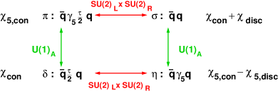
Figure 5: Symmetry transformations relating scalar and pseudo-scalar mesons, from [30].

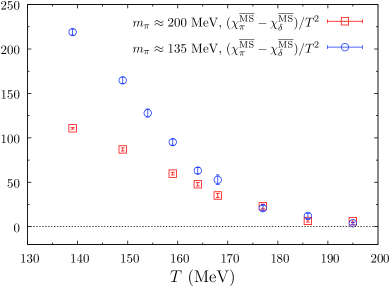
Figure 6: The chiral, $\chi_{\pi}-\chi_{\sigma}$ and $\chi_{\eta}-\chi_{\delta}$ (left), and the axial, $\chi_{\pi}-\chi_{\delta}$ (right), symmetry-breaking differences with domain-wall fermions [21].

While lattice simulations with staggered fermions suggest that the transition in 2+1 flavor QCD in the limit of vanishing light quark masses, $m_{l}\to 0$, is of second order and belongs to the $O(4)$ universality class, the nature of this transition is far from settled. This is due to the effect of the axial anomaly on the finite-temperature transition. The full symmetry group of the classical massless Lagrangian is $SU(2)_{L}\times SU(2)_{R}\times U_{V}(1)\times U_{A}(1)$, however the axial $U_{A}(1)$ symmetry is anomalous and is broken on the quantum level [31, 32]. If the $U_{A}(1)$ symmetry remains significantly broken around the chiral transition, then $O(4)$ universality class is appropriate, but if it is effectively restored, the transition may be of first order [33] or second order, but in a different universality class [34]. The strength of symmetry breaking can be analyzed from the behavior of susceptibilities, which are the 4-volume integrals of the two-point correlation functions in various channels, e.g. $\chi_{\pi}=\int d^{4}x\langle\pi(0)\pi(x)\rangle$ for the pion. Restoration of a symmetry would lead to degeneracy in the spectrum, and the symmetry transformations relating pseudo-scalar and scalar mesons are shown in Fig. 5.

The HotQCD collaboration reported [21] results on the chiral symmetry-breaking differences $\chi_{\pi}-\chi_{\sigma}$ and $\chi_{\eta}-\chi_{\delta}$, Fig. 6 (left) and $U_{A}(1)$-breaking difference $\chi_{\pi}-\chi_{\delta}$, Fig 6 (right) with domain-wall fermions at the physical pion mass. While $\chi_{\pi}-\chi_{\sigma}$ is large below $T_{c}$, it becomes zero for $T>164$ MeV, indicating restoration of the chiral symmetry. On the contrary, the $U_{A}(1)$ difference remains large at $T_{c}$, indicating no restoration of this symmetry until at least $T>196$ MeV.

The $U_{A}(1)$ breaking difference can be related to the spectral density $\rho(\lambda)$ of the eigenvalues of the Dirac operator as

$$\chi_{\pi}-\chi_{\delta}=\lim_{m\to 0}\int_{0}^{\infty}d\lambda\rho(\lambda)\frac{4m^{2}}{(m^{2}+\lambda^{2})^{2}}.$$ (2)

The JLQCD collaboration studied the spectrum of the Dirac operator with the Möbius domain-wall and overlap fermions [35, 36]. The results seem to support their earlier findings [37] that $\rho(\lambda)$ starts with cubic powers of $\lambda$ and when the chiral symmetry is restored, the $\chi_{\pi}-\chi_{\delta}$ difference becomes insensitive to the axial symmetry breaking, and that the axial symmetry may be effectively restored close to $T_{c}$. Future work may be needed to clarify the fate of the $U_{A}(1)$ symmetry and the nature of the transition in the chiral limit.

4 Fluctuations of conserved charges

A powerful tool to explore the crossover region and the nature of the degrees of freedom in the deconfined phase is fluctuations and correlations of various conserved charges. We can define generalized susceptibilities as derivatives of the pressure:

$$\chi_{klmn}^{BQSC}=\left.\frac{\partial^{(k+l+m+n)}[p(\hat{\mu}_{B},\hat{\mu}_{Q},\hat{\mu}_{S},\hat{\mu}_{C})/T^{4}]}{\partial\hat{\mu}_{B}^{k}\partial\hat{\mu}_{Q}^{l}\partial\hat{\mu}_{S}^{m}\partial\hat{\mu}_{C}^{n}}\right|_{\mu=0}$$ (3)

where $\hat{\mu}_{i}=\mu_{i}/T$, $i=B,Q,S,C$ are the dimensionless chemical potentials for the baryon number, electric charge, strangeness and charm, respectively. (We use a convention to drop a superscript in $\chi_{klmn}^{BQSC}$ when the corresponding subscript is zero.)

At low temperature fluctuations of various charges are suppressed due to confinement, while at high temperature they should approach ideal quark gas values. It has been recently shown how the electric charge fluctuations can be used for ab initio determination of the freeze-out parameters (i.e. values of the temperature, $T^{f}$, and baryon chemical potential, $\mu_{B}^{f}$, at which system hadronizes at the end of the evolution in heavy-ion collisions) [38, 39] and also to probe the strangeness carrying degrees of freedom in the high-temperature phase [40, 41]. These results have been summarized in the last year’s review by Szabo [42].

There are several new developments this year. The electric charge fluctuations are of particular interest, because they can be measured well in the heavy-ion experiments. Unfortunately, in calculations with staggered fermions they are the most sensitive to the taste breaking effects and require substantial computational effort for full control of the continuum limit. The Wuppertal-Budapest collaboration reported about ongoing calculations of $\chi^{Q}_{2}$ and $\chi^{Q}_{4}$ and attempts of continuum extrapolation [43]. The BNL-Bielefeld-CCNU collaboration continued calculations of the sixth-order cumulants with the aim of determining possible critical behavior and exploring the QCD phase diagram [44].

The phenomenology of heavy-ion collisions provides strong evidence [45] that the thermodynamics of the hadronic phase up to about the chiral crossover temperature can be well described by a gas of uncorrelated hadrons and resonances – the Hadron Resonance Gas (HRG) model [46]. The HRG partition function is a product of individual partition functions of all states in the QCD spectrum, often approximated by taking all known states from the particle data tables (PDG) [47].

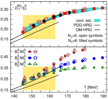
Figure 7: Ratios of susceptibilities (top) and linear combinations of susceptibilities that project baryonic and mesonic sectors (bottom) calculated on the lattice (symbols) and in the hadron resonance gas model with the PDG spectrum (solid lines) and with the spectrum predicted by the quark model (dotted lines). The HRG with the PDG spectrum significantly underpredicts the lattice data [51].

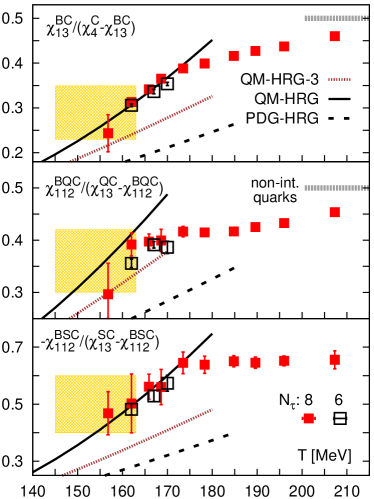
Figure 8: Similar to Fig. 8 for observables that include the charm quark [52].

It has been noted that certain quantities, such as strangeness fluctuations and correlations of strangeness and baryon number, are larger in QCD than in HRG with PDG spectrum [48, 49], and argued that these differences provide evidence for contribution of additional, not yet observed experimentally, hadron resonances. The BNL-Bielefeld-CCNU collaboration reported [50] their findings [51, 52] on the possible thermodynamic relevance of these states. Out of various generalized susceptibilities, Eq. (3), calculated on the lattice with HISQ fermions and two cutoffs, $N_{\tau}=6$ and $8$, they construct combinations, that project on various baryon number and strangeness sectors. The results are then compared with two versions of the HRG model: with spectrum taken from PDG and with the one that includes states predicted by quark model calculations, Fig. 8 and 8. Clearly, including the additional states provides a much better description of the lattice data. This also has implications for the determination of the freeze-out temperature for strange hadrons [52].

While at low temperature the susceptibilities help to test the HRG model, and in the transition region indicate a switch in the dominant degrees of freedom in the system, at high temperatures, deeply in the deconfined phase, they should eventually reach perturbative behavior. A recent calculation of the second (in the continuum) and fourth (at several cutoffs) order quark number susceptibilities indicates reasonable agreement with weak-coupling expansions for $T\gtrsim 400$ MeV [53], given the uncertainties of the latter. However, more work is needed for controlling the cutoff effects and taking the continuum limit for the fourth-order susceptibilities at high temperature.

5 The equation of state

A change from the confined into the deconfined phase is signaled by the rapid increase in the pressure, $p$, and energy density, $\epsilon$. These quantities signal deconfinement of the degrees of freedom with quantum numbers of quarks and gluons and approach the Stefan-Boltzmann limit at asymptotically high temperatures.

A lattice calculation of the equation of state usually starts with evaluation of the trace of the energy-momentum tensor, also called the trace anomaly, or the interaction measure:

$$\frac{\Theta^{\mu\mu}(T)}{T^{4}}=\frac{\epsilon-3p}{T^{4}}=T\frac{d}{dT}\left(\frac{p}{T^{4}}\right).$$ (4)

The pressure can then be calculated by integrating the trace anomaly, starting from some reference value $p_{0}(T_{0})$:

$$\frac{p(T)}{T^{4}}=\frac{p_{0}}{T_{0}^{4}}+\int_{T_{0}}^{T}dT^{\prime}\frac{\Theta^{\mu\mu}}{T^{\prime 5}}.$$ (5)

All other thermodynamic quantities that are derivatives of the partition function with respect to the temperature can be calculated from Eqs. (4) and (5), using various thermodynamic identities.

5.1 $N_{f}=0$

What makes the calculation of the equation of state on the lattice numerically expensive is the additive renormalization arising from the breaking of the Lorentz symmetry by the lattice. For every value of the gauge coupling one needs to evaluate a zero-temperature subtraction for the trace anomaly. The fixed-scale approach can potentially reduce the cost of zero-temperature calculations, since in this scheme the temperature $T=1/(aN_{\tau})$ is varied by changing $N_{\tau}$ at fixed $a$ (so only one zero-temperature calculation is needed for several temperatures). Possible temperatures are then limited by a few integer values of $N_{\tau}$.

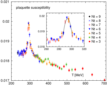
Figure 9: The plaquette susceptibility (left) and the trace anomaly (right) for $SU(3)$ pure gauge theory, calculated at one lattice spacing using shifted boundary conditions.

By using recently proposed shifted boundary conditions [54]

$$U_{4}(\vec{x},N_{\tau})=U_{4}(\vec{x}+\vec{s},0),$$ (6)

where $U$ is the gauge link variable, $N_{\tau}$ is the temporal extent of the lattice and $\vec{s}$ is the shift vector, one can cover more temperatures, $T=1/\sqrt{a^{2}N_{\tau}^{2}+\vec{s}^{2}}$, by varying $\vec{s}$ in conjunction with $N_{\tau}$. A calculation for $SU(3)$ pure gauge theory at single lattice spacing of about $0.1$ fm has been recently reported [55]. The plaquette susceptibility, used to determine $T_{c}=293$ MeV, is shown in Fig. 9 (left) and the trace anomaly in Fig. 9 (right) together with the continuum result of Ref. [56].

5.2 $N_{f}=2$

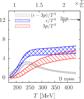
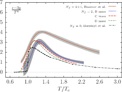
Figure 10: Left: The trace anomaly, energy density and pressure for two flavors of twisted mass Wilson fermions at $m_{\pi}=360$ MeV. Right: The trace anomaly for two flavors of twisted mass Wilson fermions at three values of $m_{\pi}$ compared with the pure gauge and 2+1 flavor staggered results.

The tmfT collaboration made progress in calculation of the equation of state with two flavors of twisted mass Wilson fermions [57]. The simulations were performed at three values of the pion mass, $m_{\pi}=360$, $430$ and $640$ MeV and the continuum limit was taken. The results for the trace anomaly, pressure and energy density for the lowest pion mass are shown in Fig. 10 (left). Around 400 MeV the energy density and pressure reach only about half of the Stefan-Boltzmann limit value. And in Fig. 10 (right) the two-flavor trace anomaly for three pion masses is compared with the pure gauge [56] and 2+1 flavor [58] results.

5.3 $N_{f}=2+1$

For 2+1 flavor QCD the equation of state is now available at the physical pion mass in the continuum limit from the Wuppertal-Budapest collaboration [59] that used stout fermions and the HotQCD collaboration [58] that used HISQ. A comparison of these results for the trace anomaly, pressure and entropy density, $s=(\epsilon+p)/T$, is shown in Fig. 12. In general, there is good agreement between them, with deviation of about $2\sigma$ in the integrated quantities arising around 400 MeV. In Fig. 12 the HISQ results for the pressure, energy and entropy density are compared with the HRG results. The yellow-shaded box represents the chiral crossover region.

Figure 11: Comparison of the continuum results for the trace anomaly, pressure and entropy density for the stout and HISQ action.

Figure 12: Comparison of the pressure, energy and entropy density calculated with HISQ with the HRG results.

The second-order derivatives of the free energy can also be constructed, the specific heat is

$$C_{V}=\left.\frac{\partial\epsilon}{\partial T}\right|_{V}\equiv\left(4\frac{\epsilon}{T^{4}}+\left.T\frac{\partial(\epsilon/T^{4})}{\partial T}\right|_{V}\right)T^{3},$$ (7)

where the second term is related to the trace anomaly and its derivative:

$$T\frac{d(\epsilon/T^{4})}{dT}=3\frac{\Theta^{\mu\mu}}{T^{4}}+T\frac{d(\Theta^{\mu\mu}/T^{4})}{dT},$$ (8)

and the speed of sound is

$$c_{s}^{2}=\frac{\partial p}{\partial\epsilon}=\frac{\partial p/\partial T}{\partial\epsilon/\partial T}=\frac{s}{C_{V}}.$$ (9)

The speed of sound is of phenomenological interest, because the softest point of the equation of state, i.e. where the speed of sound reaches the minimum, corresponds to the temperature and energy density range where the system spends longer time and the expansion and cooling of matter slows down. For this reason one may expect to observe characteristic signatures from this stage of the evolution of QGP in heavy-ion collisions [60]. The speed of sound is shown in Fig. 14. It appears that the softest point is reached at the low side of the crossover region, at $T\simeq(145-150)$ MeV.

Figure 13: The speed of sound for the stout and HISQ action compared with HRG.

Figure 14: Pressure calculated with HISQ, in the EQCD and in HTL perturbation theory.

The lattice equation of state can now be compared with the perturbative calculations to determine at what temperature weak-coupling expansions may be trusted. In Fig. 14 the pressure is compared with the perturbative calculations in the Hard Thermal Loop (HTL) [61] and Electrostatic QCD (EQCD) [62] schemes. Given the large uncertainty from varying the scale in the HTL calculation, the results generally agree, but it appears that lattice calculations at higher temperatures will be needed to reliably connect the lattice equation of state to a perturbative one and determine which, HTL or EQCD calculation, describes the equation of state better.

5.4 $N_{f}=2+1+1$

Figure 15: The 2+1+1 flavor trace anomaly with the 4stout action together with the 2+1 flavor continuum and HTL results.

Figure 16: Pressure in 2+1+1 flavor QCD with the 4stout action together with the 2+1 flavor continuum and HRG results.

Apart from presenting their final result on the 2+1 flavor equation of state [59], the Wuppertal-Budapest collaboration has also extended their calculation of the 2+1+1 flavor equation of state [63]. For the latter case they use the stout action with four levels of smearing, called 4stout (while two levels of smearing were used in the previous work). They show that at $T=214$ MeV the value of the trace anomaly with and without the dynamical charm is the same, in line with the perturbative observation that the charm contribution starts to matter around 300 MeV [62]. The 2+1+1 flavor trace anomaly with the 4stout action at $N_{\tau}=6$, $8$ and $10$ is shown in Fig. 16 and compared with the continuum 2+1 flavor result and the perturbative HTL calculation. To cover a wide temperature range $300<T<1000$ MeV and set the line of constant physics, the range of gauge couplings is split into three regions. The lattice scale is then set in different ways: from spectroscopy at coarse lattices, from simulations at the $m_{l}=m_{s}$ flavor symmetric point at intermediate lattices and from the $w_{0}$ scale determined with the Wilson flow [64] at fine lattices. The results for the pressure are shown in Fig. 16.

5.5 $N_{f}=2+1$, $\mu_{B}>0$

The susceptibilities defined in Eq. (3) are the coefficients of the Taylor expansion of the pressure with respect to the chemical potentials, and they can be used to extend the equation of state to non-zero baryon chemical potential. The BNL-Bielefeld-CCNU collaboration calculated the pressure and energy density at $O(\mu_{B}^{4})$ at several values of the chemical potential up to $\mu_{B}/T=2$, by measuring the second and fourth order susceptibilities to very high precision at $N_{\tau}=6$ and $8$ lattices with the HISQ action [65]. The results for the pressure are shown in Fig. 17 (left). By using a parametrization of the freeze-out curve that relates $(T^{f},\mu_{B}^{f})$ to the beam energy $s_{NN}^{1/2}$ [66] the equation of state can also be calculated along that curve. The pressure on the freeze-out curve is shown in Fig. 17 (right). The fourth-order equation of state can be useful down to beam energy $s_{NN}^{1/2}\sim 20$ GeV, while below that energy higher-order terms will be needed for correct description.

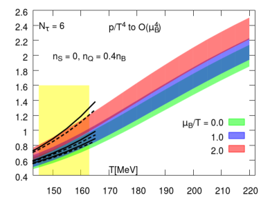
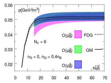
Figure 17: Left: Pressure at $O(\mu_{B}^{4})$ on $N_{\tau}=6$ lattice with HISQ. The electric charge to baryon number ratio is set to 0.4, similar to the one encountered in heavy-ion collision experiments. Right: Pressure at various orders in $\mu_{B}$ on the freeze-out curve, on $N_{\tau}=6$ lattice with HISQ.

6 In-medium properties of mesons

While the dynamics of the chiral crossover in QCD is determined by the light degrees of freedom, heavy quarks play a special role in understanding the properties of the deconfined medium. In heavy-ion collisions heavy quarks are created at the early stages of the quark-gluon plasma formation and can serve as probes of the medium. Melting of the heavy-quark bound states due to the color screening in the plasma was suggested as a signature of QGP formation [67].

Consider a local mesonic operator of the form:

$$J_{H}(t,\vec{x})=\bar{q}(t,\vec{x})\Gamma_{H}q(t,\vec{x})$$ (10)

where $q(t,\vec{x})$ is the quark field operator and $\Gamma_{H}$ denotes possible $\gamma$-matrix structure of the state (e.g. pseudoscalar, vector, etc.).

Defining the real time two-point functions of the currents (10):

$$D^{>}_{H}(t,\vec{x})=\langle J_{H}(t,\vec{x})J_{H}(0,\vec{0})\rangle,\,\,\,\,\,D^{<}_{H}(t,\vec{x})=\langle J_{H}(0,\vec{0})J_{H}(t,\vec{x})\rangle,t>0$$ (11)

and making the Fourier transform

$$D^{>(<)}_{H}(\omega,\vec{p})=\int_{-\infty}^{\infty}dt\int d^{3}xe^{i\omega t-i\vec{p}\cdot\vec{x}}D^{>(<)}_{H}(t,\vec{x})$$ (12)

we can define the spectral function

$$\rho(\omega,\vec{p})=\frac{1}{2\pi}(D^{>}_{H}(\omega,\vec{p})-D^{<}_{H}(\omega,\vec{p})).$$ (13)

Most of the dynamic properties of the state and its behavior in the medium are encoded in the spectral function. A stable state of mass $M$ contributes a $\delta$-function peak of the form:

$$\rho(\omega,\vec{p})=|\langle 0|J_{H}|H\rangle|^{2}\theta(\omega)\delta(p^{2}-M^{2}).$$ (14)

Broadening of such a peak with increasing temperature describes thermal modification of the state, and its disappearance signals melting of the state. Evaluation of the spectral function requires calculating real time two-point functions, to which lattice does not have direct access. Instead, lattice simulations are done in Euclidean space-time and produce Euclidean correlation functions:

$$G(\tau,\vec{p})=\int d^{3}xe^{i\vec{p}.\vec{x}}\langle J_{H}(\tau,\vec{x})J_{H}(0,\vec{0})\rangle,$$ (15)

which are analytic continuations of $D^{>}_{H}(t,\vec{p})$ as

$$G(\tau,\vec{p})=D^{>}_{H}(-i\tau,\vec{p}).$$ (16)

The relation between the Euclidean correlator and the spectral function is more complicated:

$$G(\tau,\vec{p}) = \int_{0}^{\infty}d\omega\rho(\omega,\vec{p})K(\omega,\tau),$$ (17)

$$K(\omega,\tau) = \frac{\cosh(\omega(\tau-1/2T))}{\sinh(\omega/2T)},$$ (18)

and, unlike the Fourier transform, does not allow for direct inversion.

To reconstruct the spectral function $\rho(\omega,\vec{p})$ from the correlator in the l.h.s. of Eq. (17) (or, in other words, solve the integral equation for $\rho$), Bayesian techniques are often employed, that try to maximize the conditional probability $P[\rho|DH]$ that $\rho(\omega,\vec{p})$ is the correct spectral function given data $D$ and some prior knowledge $H$. One of such techniques, often applied to this problem, is the Maximum Entropy Method (MEM) [68]. In this method the Shannon-Janes entropy:

$$S=\int d\omega\left[\rho(\omega)-m(\omega)-\rho(\omega)\ln\left(\frac{\rho(\omega)}{m(\omega)}\right)\right]$$ (19)

incorporates the positivity of the spectral function and all other prior knowledge is parametrized by $m(\omega)$, which is called the default model. The conditional probability is then

$$P[\rho|DH]=\exp\left(-\frac{1}{2}\chi^{2}+\alpha S\right),$$ (20)

where $\alpha$ is a real parameter.

6.1 Charmonium spectral functions

Ikeda et al. [69] developed a modification of MEM to study charmonium spectral functions at finite momentum. Using quenched QCD configurations and Wilson fermions in the valence sector they calculated charmonium correlators in the pseudoscalar channel ($\eta_{c}$). Working on anisotropic lattices $a_{\sigma}/4=a_{\tau}=0.00975$ fm they covered a temperature range $(0.78-1.78)T_{c}$. The spectral function of $\eta_{c}$ at several temperatures is shown in Fig. 18 (left). Presence of a well pronounced peak at $1.7T_{c}$ is interpreted as survival of the $\eta_{c}$ state up to that temperature. Having the spectral function allows for calculating the dispersion relation, defined in this case as the dependence of the peak position on momentum $p$. This dispersion relation is shown in Fig. 18 (right) and it seems to be described by the vacuum form $\omega=\sqrt{m^{2}+p^{2}}$ up to $1.7T_{c}$.

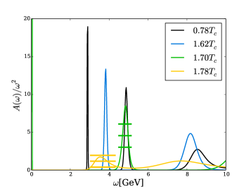
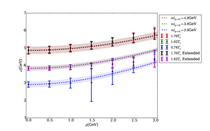
Figure 18: Left: Spectral function in the $\eta_{c}$ channel for several values of $T$. Right: Dispersion relation of $\eta_{c}$ at three temperatures [69].

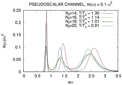
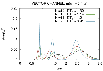
Figure 19: Temperature dependence of spectral functions in the $\eta_{c}$ (left) and $J/\psi$ (right) channel [70].

The Wuppertal-Budapest collaboration calculated the charmonium spectral functions in the pseudoscalar and vector channels using 2+1 flavors of dynamical Wilson quarks with the pion mass $m_{\pi}=545$ MeV [70]. They employed isotropic lattices down to $0.057$ fm. The results are shown in Fig. 19. Apart from the reconstruction of the spectral functions with MEM, the analysis of the Euclidean correlators was also performed, leading to a conclusion that no melting of $\eta_{c}$ and $J/\psi$ mesons was observed up to a temperature of $1.4T_{c}$.

6.2 Bottomonium spectral functions

The bottom quark is substantially heavier and controlling the discretization errors is harder, therefore effective theories are often used.

The FASTSUM collaboration performed a calculation of the bottomonium spectral functions with MEM using Non-Relativistic QCD (NRQCD) [71] for the bottom quark. For the gauge background they used 2+1 flavors of clover improved Wilson quarks with the pion mass $m_{\pi}=400$ MeV. The spectral functions for $S$- and $P$-wave channels ($\Upsilon$ and $\chi_{b1}$ mesons) are shown in Fig. 20. The ground state peak in the $S$-wave case, present at all temperatures, indicates the survival of $\Upsilon$ up to the highest temperature of $1.9T_{c}$. In the $P$-wave case disappearance of the peak is observed slightly above $T_{c}$, indicating dissociation of $\chi_{b1}$ once the deconfined phase is reached.

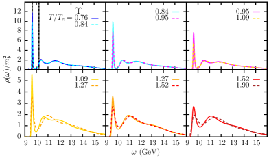
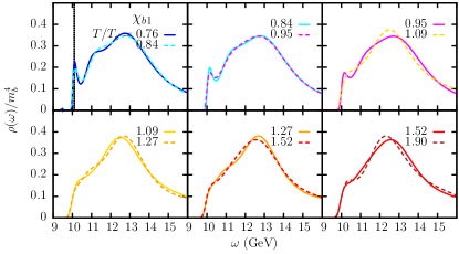
Figure 20: Temperature dependence of spectral functions in the $\Upsilon$ (left) and $\chi_{b1}$ (right) channel [71].

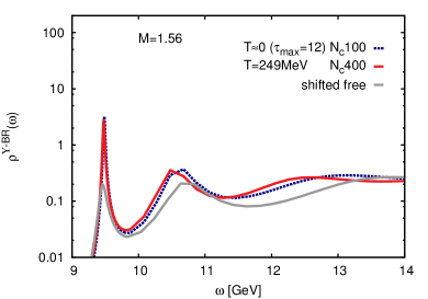
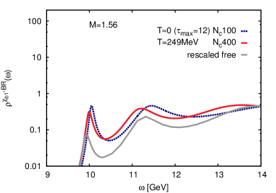
Figure 21: $\Upsilon$ (left) and $\chi_{b1}$ (right) spectral functions at $T=0$ and $249$ MeV [72, 73].

Kim et al. [72, 73] calculated the bottomonium spectral functions also employing NRQCD for the bottom quark, but on a different gauge background of 2+1 flavors of highly improved staggered quarks with the pion mass $m_{\pi}=160$ MeV. They also used a different Bayesian approach, recently suggested in Ref. [74]. The $S$- and $P$-wave spectral functions at $T=0$ and $T=249$ MeV are shown in Fig. 21. In this case, contrary to the finding of the previous group, the $P$-wave state features a peak at $T=1.6T_{c}$ (taking $T_{c}=154$ MeV), signaling no dissociation of $\chi_{b1}$ in the plasma up to that temperature. Clearly, further studies are needed to resolve the tension between these two results.

6.3 Static quark potential at finite temperature

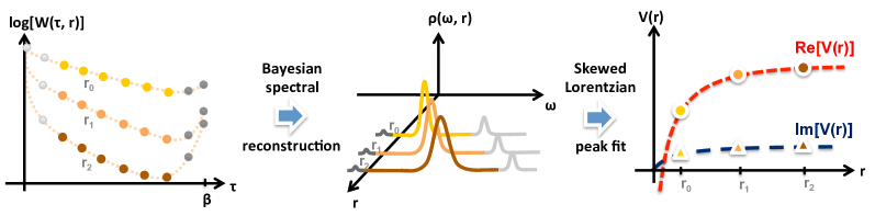
Figure 22: The strategy for extracting the imaginary part of the static quark potential by reconstructing the spectral function of a Wilson loop, from [75].

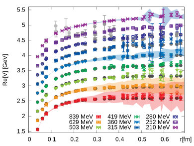
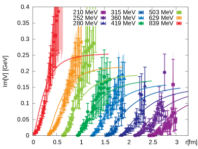
Figure 23: Real (left) and imaginary (right) part of the static quark potential in $SU(3)$ pure gauge theory.

The static quark potential at zero temperature is a well-known quantity that has been studied since the early days of lattice QCD. It is often used to set the scale in lattice calculations, since its measurement is numerically cheap. At finite temperature the color singlet free energy of a static quark anti quark pair is sometimes used as a proxy for it. The situation is, however, more involved. The potential is related to the late real-time behavior of the rectangular Wilson loop:

$$V(r)=\lim_{t\to\infty}\frac{i\partial_{t}W(t,r)}{W(t,r)},\quad W(t,r)=\left\langle{\rm exp}\Big{[}-{ig}\int_{\square}dx_{\mu}A^{\mu}(x)\Big{]}\right\rangle,$$ (21)

and, in general, it is complex valued. At finite temperature, the familiar real part describes the Debye color screening, while the imaginary part is related to the Landau damping in the plasma. Since the real-time behavior is not accessible in Euclidean lattice formalism, the imaginary part of the potential cannot be measured directly in Monte Carlo simulations. However, a strategy similar to the one used for spectral functions can be applied, as sketched in Fig. 22. By finding the spectral decomposition of the Euclidean Wilson loop

$$W(\tau,r)=\int d\omega e^{-\omega\tau}\rho(\omega,r)$$ (22)

one can use the spectral function to calculate the complex-valued potential

$$V(r)=\lim_{t\to\infty}\frac{\int d\omega\,\omega e^{-i\omega t}\rho(\omega,r)}{\int d\omega\,e^{-i\omega t}\rho(\omega,r)}.$$ (23)

Burnier et al. [75, 76] calculated Wilson line correlators in the Coulomb gauge (which are less noisy than Wilson loops) on quenched and dynamical 2+1 flavor asqtad lattices, covering the temperature range $210\leqslant T\leqslant 839$ MeV and $148\leqslant T\leqslant 248$ MeV, respectively. The results for the real and imaginary part of the potential for the quenched case are shown in Fig. 23. The real part is compared with the color singlet free energy, calculated on the lattice, and the imaginary part with the HTL result at leading order. The results for the imaginary part are consistent with the ones obtained recently by using HTL-inspired spectral functions and fitting their parameters to measured Wilson line correlators [77].

7 Summary

There have been many interesting developments in finite-temperature lattice QCD in 2014, and some of them, summarized in this review, are listed below. Calculations with domain-wall fermions confirm the staggered result on the chiral crossover temperature $T_{c}$ and favor restoration of the axial symmetry considerably above $T_{c}$. Fluctuations and correlations of conserved charges can be used to construct observables that relate to the ones measured in heavy-ion collision experiments and, in particular, efforts to calculate higher order cumulants of the electric charge are ongoing. The results on the equation of state in 2+1 flavor QCD at the physical pion mass in the continuum limit are now available and agreement between the stout and HISQ calculations is demonstrated in $130-400$ MeV range. A new method for calculating the equation of state on the lattice using non-conventional boundary conditions has been introduced and tested for $SU(3)$ pure gauge theory. Several groups continue calculations of the spectral functions for heavy quarkonia and new techniques for extracting spectral functions have been introduced.

- [1] D. J. Gross and F. Wilczek, Ultraviolet Behavior of Nonabelian Gauge Theories, Phys.Rev.Lett. 30 (1973) 1343–1346.
- [2] H. D. Politzer, Reliable Perturbative Results for Strong Interactions?, Phys.Rev.Lett. 30 (1973) 1346–1349.
- [3] C.-N. Yang and R. L. Mills, Conservation of Isotopic Spin and Isotopic Gauge Invariance, Phys.Rev. 96 (1954) 191–195.
- [4] J. C. Collins and M. Perry, Superdense Matter: Neutrons Or Asymptotically Free Quarks?, Phys.Rev.Lett. 34 (1975) 1353.
- [5] N. Cabibbo and G. Parisi, Exponential Hadronic Spectrum and Quark Liberation, Phys.Lett. B59 (1975) 67–69.
- [6] K. G. Wilson, Confinement of Quarks, Phys.Rev. D10 (1974) 2445–2459.
- [7] M. Creutz, Monte Carlo Study of Quantized SU(2) Gauge Theory, Phys.Rev. D21 (1980) 2308–2315.
- [8] L. D. McLerran and B. Svetitsky, A Monte Carlo Study of SU(2) Yang-Mills Theory at Finite Temperature, Phys.Lett. B98 (1981) 195.
- [9] J. Kuti, J. Polonyi, and K. Szlachanyi, Monte Carlo Study of SU(2) Gauge Theory at Finite Temperature, Phys.Lett. B98 (1981) 199.
- [10] J. Engels, F. Karsch, H. Satz, and I. Montvay, High Temperature SU(2) Gluon Matter on the Lattice, Phys.Lett. B101 (1981) 89.
- [11] BRAHMS Collaboration, I. Arsene et al., Quark gluon plasma and color glass condensate at RHIC? The Perspective from the BRAHMS experiment, Nucl.Phys. A757 (2005) 1–27, [nucl-ex/0410020].
- [12] PHOBOS Collaboration, B. Back, M. Baker, M. Ballintijn, D. Barton, B. Becker, et al., The PHOBOS perspective on discoveries at RHIC, Nucl.Phys. A757 (2005) 28–101, [nucl-ex/0410022].
- [13] STAR Collaboration, J. Adams et al., Experimental and theoretical challenges in the search for the quark gluon plasma: The STAR Collaboration’s critical assessment of the evidence from RHIC collisions, Nucl.Phys. A757 (2005) 102–183, [nucl-ex/0501009].
- [14] PHENIX Collaboration, K. Adcox et al., Formation of dense partonic matter in relativistic nucleus-nucleus collisions at RHIC: Experimental evaluation by the PHENIX collaboration, Nucl.Phys. A757 (2005) 184–283, [nucl-ex/0410003].
- [15] MILC Collaboration, C. Bernard et al., QCD thermodynamics with three flavors of improved staggered quarks, Phys.Rev. D71 (2005) 034504, [hep-lat/0405029].
- [16] M. Cheng, N. Christ, S. Datta, J. van der Heide, C. Jung, et al., The Transition temperature in QCD, Phys.Rev. D74 (2006) 054507, [hep-lat/0608013].
- [17] Y. Aoki, G. Endrodi, Z. Fodor, S. Katz, and K. Szabo, The Order of the quantum chromodynamics transition predicted by the standard model of particle physics, Nature 443 (2006) 675–678, [hep-lat/0611014].
- [18] H.-T. Ding, F. Karsch, and S. Mukherjee, Thermodynamics of strong-interaction matter from Lattice QCD, arXiv:1504.05274.
- [19] D. Sexty, New algorithms for finite density QCD, arXiv:1410.8813.
- [20] F. R. Brown, F. P. Butler, H. Chen, N. H. Christ, Z.-h. Dong, et al., On the existence of a phase transition for QCD with three light quarks, Phys.Rev.Lett. 65 (1990) 2491–2494.
- [21] T. Bhattacharya, M. I. Buchoff, N. H. Christ, H.-T. Ding, R. Gupta, et al., QCD Phase Transition with Chiral Quarks and Physical Quark Masses, Phys.Rev.Lett. 113 (2014), no. 8 082001, [arXiv:1402.5175].
- [22] A. Bazavov, T. Bhattacharya, M. Cheng, C. DeTar, H. Ding, et al., The chiral and deconfinement aspects of the QCD transition, Phys.Rev. D85 (2012) 054503, [arXiv:1111.1710].
- [23] S. Borsanyi, S. Durr, Z. Fodor, C. Holbling, S. D. Katz, et al., QCD thermodynamics with continuum extrapolated Wilson fermions II, arXiv:1504.03676.
- [24] Y. Aoki, S. Borsanyi, S. Durr, Z. Fodor, S. D. Katz, et al., The QCD transition temperature: results with physical masses in the continuum limit II., JHEP 0906 (2009) 088, [arXiv:0903.4155].
- [25] Wuppertal-Budapest Collaboration, S. Borsanyi et al., Is there still any mystery in lattice QCD? Results with physical masses in the continuum limit III, JHEP 1009 (2010) 073, [arXiv:1005.3508].
- [26] C. Morningstar and M. J. Peardon, Analytic smearing of SU(3) link variables in lattice QCD, Phys.Rev. D69 (2004) 054501, [hep-lat/0311018].
- [27] HPQCD, UKQCD Collaboration, E. Follana et al., Highly improved staggered quarks on the lattice, with applications to charm physics, Phys.Rev. D75 (2007) 054502, [hep-lat/0610092].
- [28] D. B. Kaplan, A Method for simulating chiral fermions on the lattice, Phys.Lett. B288 (1992) 342–347, [hep-lat/9206013].
- [29] V. Furman and Y. Shamir, Axial symmetries in lattice QCD with Kaplan fermions, Nucl.Phys. B439 (1995) 54–78, [hep-lat/9405004].
- [30] HotQCD Collaboration, A. Bazavov et al., The chiral transition and symmetry restoration from lattice QCD using Domain Wall Fermions, Phys.Rev. D86 (2012) 094503, [arXiv:1205.3535].
- [31] S. L. Adler, Axial vector vertex in spinor electrodynamics, Phys.Rev. 177 (1969) 2426–2438.
- [32] J. Bell and R. Jackiw, A PCAC puzzle: pi0 –¿ gamma gamma in the sigma model, Nuovo Cim. A60 (1969) 47–61.
- [33] R. D. Pisarski and F. Wilczek, Remarks on the Chiral Phase Transition in Chromodynamics, Phys.Rev. D29 (1984) 338–341.
- [34] A. Pelissetto and E. Vicari, Relevance of the axial anomaly at the finite-temperature chiral transition in QCD, Phys.Rev. D88 (2013), no. 10 105018, [arXiv:1309.5446].
- [35] JLQCD Collaboration, G. Cossu et al., Axial U(1) symmetry at finite temperature with Möbius domain-wall fermions, arXiv:1412.5703.
- [36] A. Tomiya, G. Cossu, H. Fukaya, S. Hashimoto, and J. Noaki, Effects of near-zero Dirac eigenmodes on axial U(1) symmetry at finite temperature, arXiv:1412.7306.
- [37] S. Aoki, H. Fukaya, and Y. Taniguchi, Chiral symmetry restoration, eigenvalue density of Dirac operator and axial U(1) anomaly at finite temperature, Phys.Rev. D86 (2012) 114512, [arXiv:1209.2061].
- [38] A. Bazavov, H. Ding, P. Hegde, O. Kaczmarek, F. Karsch, et al., Freeze-out Conditions in Heavy Ion Collisions from QCD Thermodynamics, Phys.Rev.Lett. 109 (2012) 192302, [arXiv:1208.1220].
- [39] S. Borsanyi, Z. Fodor, S. Katz, S. Krieg, C. Ratti, et al., Freeze-out parameters: lattice meets experiment, Phys.Rev.Lett. 111 (2013) 062005, [arXiv:1305.5161].
- [40] A. Bazavov, H. T. Ding, P. Hegde, O. Kaczmarek, F. Karsch, et al., Strangeness at high temperatures: from hadrons to quarks, Phys.Rev.Lett. 111 (2013) 082301, [arXiv:1304.7220].
- [41] R. Bellwied, S. Borsanyi, Z. Fodor, S. D. Katz, and C. Ratti, Is there a flavor hierarchy in the deconfinement transition of QCD?, Phys.Rev.Lett. 111 (2013) 202302, [arXiv:1305.6297].
- [42] K. Szabo, QCD at non-zero temperature and magnetic field, PoS LATTICE2013 (2014) 014, [arXiv:1401.4192].
- [43] S. Borsanyi, “Fluctuations of the electric charge in theory and experiment.” Unpublished, see contribution 240 at http://www.bnl.gov/lattice2014, 2014.
- [44] C. Schmidt, “Exploring the QCD phase diagram with conserved charge fluctuations.” These proceedings, 2014.
- [45] P. Braun-Munzinger, K. Redlich, and J. Stachel, Particle production in heavy ion collisions, nucl-th/0304013.
- [46] R. Hagedorn, Statistical thermodynamics of strong interactions at high-energies, Nuovo Cim.Suppl. 3 (1965) 147–186.
- [47] Particle Data Group Collaboration, J. Beringer et al., Review of Particle Physics (RPP), Phys.Rev. D86 (2012) 010001.
- [48] S. Borsanyi, Z. Fodor, S. D. Katz, S. Krieg, C. Ratti, et al., Fluctuations of conserved charges at finite temperature from lattice QCD, JHEP 1201 (2012) 138, [arXiv:1112.4416].
- [49] HotQCD Collaboration, A. Bazavov et al., Fluctuations and Correlations of net baryon number, electric charge, and strangeness: A comparison of lattice QCD results with the hadron resonance gas model, Phys.Rev. D86 (2012) 034509, [arXiv:1203.0784].
- [50] BNL-Bielefeld-CCNU Collaboration, H.-T. Ding, Thermodynamics of heavy-light hadrons, arXiv:1412.5735.
- [51] A. Bazavov, H.-T. Ding, P. Hegde, O. Kaczmarek, F. Karsch, et al., The melting and abundance of open charm hadrons, Phys.Lett. B737 (2014) 210–215, [arXiv:1404.4043].
- [52] A. Bazavov, H. T. Ding, P. Hegde, O. Kaczmarek, F. Karsch, et al., Additional Strange Hadrons from QCD Thermodynamics and Strangeness Freezeout in Heavy Ion Collisions, Phys.Rev.Lett. 113 (2014), no. 7 072001, [arXiv:1404.6511].
- [53] A. Bazavov, H.-T. Ding, P. Hegde, F. Karsch, C. Miao, et al., Quark number susceptibilities at high temperatures, Phys.Rev. D88 (2013), no. 9 094021, [arXiv:1309.2317].
- [54] L. Giusti and H. B. Meyer, Thermal momentum distribution from path integrals with shifted boundary conditions, Phys.Rev.Lett. 106 (2011) 131601, [arXiv:1011.2727].
- [55] T. Umeda, Fixed-scale approach to finite-temperature lattice QCD with shifted boundaries, Phys.Rev. D90 (2014), no. 5 054511, [arXiv:1408.2328].
- [56] S. Borsanyi, G. Endrodi, Z. Fodor, S. Katz, and K. Szabo, Precision SU(3) lattice thermodynamics for a large temperature range, JHEP 1207 (2012) 056, [arXiv:1204.6184].
- [57] tmfT Collaboration, F. Burger, E.-M. Ilgenfritz, M. P. Lombardo, and M. Müller-Preussker, Equation of state of quark-gluon matter from lattice QCD with two flavors of twisted mass Wilson fermions, Phys.Rev. D91 (2015), no. 7 074504, [arXiv:1412.6748].
- [58] HotQCD Collaboration, A. Bazavov et al., Equation of state in ( 2+1 )-flavor QCD, Phys.Rev. D90 (2014), no. 9 094503, [arXiv:1407.6387].
- [59] S. Borsanyi, Z. Fodor, C. Hoelbling, S. D. Katz, S. Krieg, et al., Full result for the QCD equation of state with 2+1 flavors, Phys.Lett. B730 (2014) 99–104, [arXiv:1309.5258].
- [60] C. Hung and E. V. Shuryak, Hydrodynamics near the QCD phase transition: Looking for the longest lived fireball, Phys.Rev.Lett. 75 (1995) 4003–4006, [hep-ph/9412360].
- [61] N. Haque, A. Bandyopadhyay, J. O. Andersen, M. G. Mustafa, M. Strickland, et al., Three-loop HTLpt thermodynamics at finite temperature and chemical potential, JHEP 1405 (2014) 027, [arXiv:1402.6907].
- [62] M. Laine and Y. Schroder, Quark mass thresholds in QCD thermodynamics, Phys.Rev. D73 (2006) 085009, [hep-ph/0603048].
- [63] S. Borsanyi, Z. Fodor, C. Hoelbling, S. D. Katz, S. Krieg, et al., Recent results on the Equation of State of QCD, arXiv:1410.7917.
- [64] M. Lüscher, Properties and uses of the Wilson flow in lattice QCD, JHEP 1008 (2010) 071, [arXiv:1006.4518].
- [65] BNL-Bielefeld-CCNU Collaboration, P. Hegde, The QCD equation of state to , arXiv:1412.6727.
- [66] J. Cleymans and K. Redlich, Chemical and thermal freezeout parameters from 1-A/GeV to 200-A/GeV, Phys.Rev. C60 (1999) 054908, [nucl-th/9903063].
- [67] T. Matsui and H. Satz, Suppression by Quark-Gluon Plasma Formation, Phys.Lett. B178 (1986) 416.
- [68] M. Asakawa, T. Hatsuda, and Y. Nakahara, Maximum entropy analysis of the spectral functions in lattice QCD, Prog.Part.Nucl.Phys. 46 (2001) 459–508, [hep-lat/0011040].
- [69] A. Ikeda, M. Asakawa, and M. Kitazawa, Charmonium spectra and dispersion relation with improved Bayesian analysis in lattice QCD, arXiv:1412.0357.
- [70] S. Borsanyi, S. Dürr, Z. Fodor, C. Hoelbling, S. D. Katz, et al., Spectral functions of charmonium with 2+1 flavours of dynamical quarks, arXiv:1410.7443.
- [71] G. Aarts, C. Allton, T. Harris, S. Kim, M. P. Lombardo, et al., The bottomonium spectrum at finite temperature from Nf = 2 + 1 lattice QCD, JHEP 1407 (2014) 097, [arXiv:1402.6210].
- [72] S. Kim, P. Petreczky, and A. Rothkopf, Lattice NRQCD study of S- and P-wave bottomonium states in a thermal medium with light flavors, Phys.Rev. D91 (2015) 054511, [arXiv:1409.3630].
- [73] S. Kim, P. Petreczky, and A. Rothkopf, NRQCD based S- and P-wave bottomonium spectra at finite temperature from lattices with light HISQ flavors, arXiv:1410.2110.
- [74] Y. Burnier and A. Rothkopf, Bayesian Approach to Spectral Function Reconstruction for Euclidean Quantum Field Theories, Phys.Rev.Lett. 111 (2013) 182003, [arXiv:1307.6106].
- [75] Y. Burnier, O. Kaczmarek, and A. Rothkopf, The in-medium heavy quark potential from quenched and dynamical lattice QCD, arXiv:1410.7311.
- [76] Y. Burnier, O. Kaczmarek, and A. Rothkopf, Static quark-antiquark potential in the quark-gluon plasma from lattice QCD, Phys.Rev.Lett. 114 (2015), no. 8 082001, [arXiv:1410.2546].
- [77] A. Bazavov, Y. Burnier, and P. Petreczky, Lattice calculation of the heavy quark potential at non-zero temperature, arXiv:1404.4267.