QM/MM Methods for Crystalline Defects.
Part 1: Locality of the Tight Binding Model

Abstract

The tight binding model is a minimal electronic structure model for molecular modelling and simulation. We show that the total energy in this model can be decomposed into site energies, that is, into contributions from each atomic site whose influence on their environment decays exponentially. This result lays the foundation for a rigorous analysis of QM/MM coupling schemes.

1 Introduction

QM/MM coupling methods are a class of multi-scale schemes in which a quantum mechanical (QM) simulation is “embedded” in a larger molecular mechanics (MM) simulation. Due to the high computational cost of QM models, schemes of this type have become an indispensable tool in many scientific disciplines [3, 22, 31, 38, 50, 58]. The present work is the first part in a series establishing the mathematical foundation of QM/MM schemes in the context of materials modelling.

It is pointed out in [21] that a minimal requirement for a QM model to be suitable for QM/MM coupling is the strong locality of forces,

$$\bigg{|}\frac{\partial f_{n}}{\partial y_{m}}\bigg{|}\to 0\quad\text{``sufficiently rapidly'' as }r_{nm}\to 0,$$ (1.1)

where $r_{nm}=|y_{n}-y_{m}|$ and $f_{n}$ denotes the force acting on an atom at position $y_{n}$ within a collection of nuclei at positions $\{y_{\ell}\}\subset\mathbb{R}^{d}$. The condition (1.1) is called strong locality to set it apart from the weaker condition of locality of the density matrix, which is already well understood (see e.g. [2, 33] and §1.2).

To study (1.1) we take a general tight binding method at finite electronic temperature as a model problem. We prove an even stronger condition than (1.1), strong energy locality: Given a finite collection of nuclei $y=\{y_{\ell}\}$, we decompose the total energy $E=E(y)$ into

$$E(y)=\sum_{\ell}E_{\ell}(y),$$ (1.2)

where the site energies $E_{\ell}(y)$ are local in the sense that

$$\bigg{|}\frac{\partial E_{\ell}(y)}{\partial y_{n}}\bigg{|}\lesssim e^{-\gamma r_{\ell n}},\qquad\bigg{|}\frac{\partial^{2}E_{\ell}(y)}{\partial y_{n}\partial y_{m}}\bigg{|}\lesssim e^{-\gamma(r_{\ell n}+r_{\ell m})},$$ (1.3)

for some $\gamma>0$, and analogous results for higher order derivatives. While the specific form of the decomposition we employ (cf. § 2.3) is well-known [28, 29], the locality result (1.3) is, to the best of our knowledge, new. We are only aware of one analogous result, for the Thomas–Fermi–von Weizsäcker model [48].

This locality result has a range of consequences, such as: (1) It provides a strong theoretical justification for the concept of an interatomic potential. (2) From a purely analytical point of view, there is little (if any) distinction between the tight binding model and interatomic potential models. This means that we can apply many of the analytical tools developed for interatomic potential models, for example: (3) We can rigorously formulate and analyze models of defects in infinite crystalline solids [27]. (4) We can extend the construction and analysis of atomistic/continuum multi-scale schemes. In particular, the Cauchy–Born continuum limit analysis [51] can be directly applied without additional work.

(5) Our main motivation, however, is to formulate and analyze new QM/MM coupling schemes for crystal defects. In this endeavour we build on the successful theory of atomistic/continuum coupling [46], employing the tools and language of numerical analysis. The key idea is that, due to (1.2) and (1.3), the total energy can be approximated by

$$E(y)\approx\sum_{\ell\in{\rm QM}}E_{\ell}(y)+\sum_{\ell\in{\rm MM}}\tilde{E}_{\ell}(y),$$

where $\tilde{E}_{\ell}$ is not an off-the shelf site potential (Lennard-Jones, EAM, …) as in previous works on QM/MM coupling, but instead is a controlled approximation to $E_{\ell}$. We show in the companion papers [18, 19] that this approach yields new QM/MM schemes (both energy-based and force-based) with rigorous rates of convergence in terms of the QM core region size.

1.1 Outline

In Section 2 we focus on finite systems. We first present a thorough discussion of real-space tight binding models and then establish the results (1.2) and (1.3) in this context. In Section 3 we then extend the definition of the site energy as well as the locality results to infinite systems (with an eye to crystal lattices) via a limiting procedure. In Section 4 we briefly present two applications of the locality results, both in preparation for Parts 2 and 3 of this series: We extend the crystal defect model and the convergence analysis for a truncation scheme from [27] to the tight binding model. Finally, in Section 5, we present some preliminary numerical tests illustrating our analytical results.

1.2 Further Remarks

Tight binding model. Tight binding models are minimalistic quantum mechanics type molecular models, used to investigate and predict properties of molecules and materials in condensed phases. Both in terms of accuracy and computational cost they are situated between accurate but computationally expensive ab initio methods and fast but limited empirical methods. While tight binding models are interesting in their own right, they also serve as a convenient toy model for more accurate electronic structure models such as (Kohn–Sham) density functional theory.

The study of defects in crystals is a field to which tight binding is well suited, as it is frequently the case that the deviations from ideal bonding are large enough that empirical potentials are not sufficiently accurate, but the system size required to isolate the defect (e.g. for dislocations or cracks) makes the use of ab initio calculations challenging. A number of studies have been carried out in which tight binding is applied to simulations of crystal defects, see e.g. [40, 43, 49, 56].

Weak versus strong locality. By weak locality we mean that the electron density matrix has exponentially fast off-diagonal decay. In the context of tight binding, this means

$$\big{[}\Gamma(y)\big{]}_{mn}\lesssim e^{-\gamma r_{mn}}$$ (1.4)

(see (2.29) for the definition of the tight binding density matrix $\Gamma(y)$). In physics, this is often described by the term “nearsightedness” [39, 53], which states that the electron properties of insulators and metals at finite temperature do not depend on perturbations at distant regions. This property has, e.g., been exploited to create linear scaling electronic structure algorithms [1, 7, 33, 37].

However, the weak locality is not enough to validate a hybrid QM/MM approach [21]. We need the stronger locality condition (1.1) to guarantee that the QM region is not affected by the classical particles, and moreover that the forces in the QM region can be computed to high accuracy by only considering a small QM neighbourhood. The decay rate in equation (1.3) then gives a guide to how large the QM region needs to be (see also Theorem 4.3 and [18, 19]).

Thermodynamic limit. Thermodynamic limit problems (infinite body limit), related to our analysis in Section 3, have been studied at great length in the analysis literature. The monograph [15] gives an extensive account of the major contributions and also presents the thermodynamic limit problem for the Thomas–Fermi–von Weizsäcker (TFW) model for perfect crystals. The thermodynamic limit of the reduced Hartree–Fock (rHF) is studied in [16] for perfect crystals. This literature also contains many results on the modelling of local defects in crystals in the framework of the TFW and rHF models, see e.g. [6, 8, 9, 10, 11, 12, 42, 44].

These discussions are restricted to the case where the nuclei are fixed on a periodic lattice (or with a given local defect). Leaving the positions of the nuclei free is also a case of great physical and mathematical interest. Motivated by [27] we present such a model in § 4.1, but postpone a complete analysis to [17].

A related problem is the continuum limit of quantum models. The TFW and rHF models are studied in [5, 13] where it is shown that, in the continuum limit, the difference between the energies of the atomistic and continuum models obtained using the Cauchy-Born rule tends to zero. The tight binding and Kohn–Sham models are studied in a series of papers [23, 24, 25, 26], which establish the extension of the Cauchy–Born rule for smoothly deformed crystals. Our locality result yields an immediate extension of the analysis of the Cauchy–Born model in the molecular mechanics case [51].

1.3 Notation

The symbol $\langle\cdot,\cdot\rangle$ denotes an abstract duality pairing between a Banach space and its dual. The symbol $|\cdot|$ normally denotes the Euclidean or Frobenius norm, while $\|\cdot\|$ denotes an operator norm. The constant $C$ is a generic positive constant that may change from one line of an estimate to the next. When estimating rates of decay or convergence, $C$ will always remain independent of the system size, of lattice position or of test functions. The dependencies of $C$ will normally be clear from the context or stated explicitly.

1.4 List of assumptions

Our analysis requires a number of assumptions on the tight binding model or the underlying atomistic geometry. For the reader’s convenience we list these with page references and brief summaries:

L	p. 2	uniform non-interpenetration
H.tb	p. 2.1	locality of Hamiltonian
H.loc	p. 2.1	locality of Hamiltonian derivatives
H.sym	p. 2.1	symmetries of Hamiltonian
F	p. 2.2	configuration independent distribution
U	p. 2.2	locality of the repulsive potential
H.emb	p. 3	connection between the Hamiltonians of two embedded systems
D	p. 4.1	homogeneity of the reference configuration outside a defect core

2 Tight binding model for finite systems

We begin by formulating a general tight binding model for a finite system with $N$ atoms. Let $\Lambda_{N}$ be an index set with $\#\Lambda_{N}=N$. An atomic configuration is described by a map $y:\Lambda_{N}\rightarrow\mathbb{R}^{d}$ with $d\in\mathbb{N}$ denoting the space dimension. (We admit $d\neq 3$ mostly for the sake of mathematical generality; e.g., this allows us to formulate simplified in-plane or anti-plane models.)

We say that the map $y$ is a proper configuration if the atoms do not accumulate:

L.  $\exists~{}\mathfrak{m}>0$ such that   $|y(\ell)-y(k)|\geq\mathfrak{m}~{}~{}\forall~{}\ell,k\in\Lambda_{N}$.

Let $\mathcal{V}^{N}_{\mathfrak{m}}\subset\big{(}\mathbb{R}^{d}\big{)}^{\Lambda_{N}}$ denote the subset of all $y\in(\mathbb{R}^{d})^{\Lambda_{N}}$ satisfying L.

2.1 The Hamiltonian matrix

In the tight binding formalism one constructs a Hamiltonian matrix $\mathcal{H}$ in an “atomic-like basis set” $\{\phi_{\ell\alpha}({\bf r}-y(\ell))\}_{\ell\in\Lambda_{N},\alpha\in\Xi}$,

$$\Big{(}\mathcal{H}(y)\Big{)}_{\ell k}^{\alpha\beta}=\int_{\mathbb{R}^{d}}\phi_{\ell\alpha}({\bf r}-y(\ell))\widehat{\mathcal{H}}(y)\phi_{k\beta}({\bf r}-y(k))~{}{\rm d}{\bf r},$$ (2.1)

where $\Xi$ is a small collection of the atomic orbitals per atom (with maximum size $n_{\Xi}$), and the exact many-body Hamiltonian operator $\widehat{\mathcal{H}}$ is usually replaced by a parametrized one. The entries of the Hamiltonian matrix $\mathcal{H}$ depend on the atomic species, atomic orbitals and on the configuration of nuclei. In practice, they are often described by empirical functions (empirical tight binding) which have been calibrated using experimental results or results from first principle calculations.

In either case, we can write the Hamiltonian matrix elements as

$$\Big{(}\mathcal{H}(y)\Big{)}_{\ell k}^{\alpha\beta}=h_{\ell k}^{\alpha\beta}(y),$$ (2.2)

where $h_{\ell k}^{\alpha\beta}:\mathcal{V}^{N}_{\mathfrak{m}}\rightarrow\mathbb{R}$ are functions depending on $\ell,~{}k,~{}\alpha$ and $\beta$.

The orbital indices $\alpha$, $\beta$ do not bring any additional insight into the problem we are studying, while at the same time complicating the notation. Therefore, we ignore the indices $\alpha$, $\beta$, which is equivalent to assuming that there is one atomic orbital for each atomic site ($n_{\Xi}$=1). The Hamiltonian matrix elements then simply become

$$\Big{(}\mathcal{H}(y)\Big{)}_{\ell k}=h_{\ell k}(y),$$ (2.3)

All our results can be generalized to cases with $n_{\Xi}>1$ without difficulty. The only required modification is outlined in Appendix A.

We make the following standing assumptions on the functions $h_{\ell k}(y)$, which we justify below in Remark 2.1 and Examples 2.1, 2.2. Briefly, these assumptions are consistent with most tight binding models, with the only exception that we assume that Coulomb interactions are screened.

H.tb. There exist positive constants $\bar{h}_{0}$ and $\gamma_{0}$ such that, for any $y\in\mathcal{V}^{N}_{\mathfrak{m}}$,

$$|h_{\ell k}(y)|\leq\bar{h}_{0}e^{-\gamma_{0}|y(\ell)-y(k)|}\quad\forall~{}\ell,k\in\Lambda_{N}.$$ (2.4)

H.loc. There exists $\mathfrak{n}\geq 4$ such that $h_{\ell k}\in C^{\mathfrak{n}}(\mathcal{V}^{N}_{\mathfrak{m}})$. Moreover, there exist positive constants $\bar{h}_{j}$ and $\gamma_{j}$ for $1\leq j\leq\mathfrak{n}$, such that

$$\left|\frac{\partial^{j}h_{\ell k}(y)}{\partial[y(m_{1})]_{i_{1}}\cdots\partial[y(m_{j})]_{i_{j}}}\right|\leq\bar{h}_{j}e^{-\gamma_{j}\sum_{l=1}^{j}\left(|y(\ell)-y(m_{l})|+|y(k)-y(m_{l})|\right)}\quad\forall~{}\ell,k\in\Lambda_{N}$$ (2.5)

with $m_{1},\cdots,m_{j}\in\Lambda_{N}$ and $1\leq i_{1},\dots,i_{j}\leq d$.

H.sym. (i) (Isometry invariance) If $y\in\mathcal{V}_{\mathfrak{m}}^{N}$ and $g:\mathbb{R}^{d}\rightarrow\mathbb{R}^{d}$ is an isometry, then

$$h_{\ell k}(y)=h_{\ell k}(g(y))\quad\forall~{}\ell,k\in\Lambda_{N}.$$ (2.6)

(ii) (Permutation invariance) If $y\in\mathcal{V}_{\mathfrak{m}}^{N}$ and $\mathcal{G}:\Lambda_{N}\rightarrow\Lambda_{N}$ is a permutation (relabelling) of $\Lambda_{N}$, then

$$h_{\ell k}(y)=h_{\mathcal{G}^{-1}(\ell)\mathcal{G}^{-1}(k)}(y\circ\mathcal{G})\quad\forall~{}\ell,k\in\Lambda_{N}.$$ (2.7)

Remark 2.1.

(i) Condition (2.4) indicates that all the matrix elements are bounded by $\bar{h}_{0}$, which is independent of the system size. This is reasonable under the assumption L and that the number of atomic orbitals per atom in $\Xi$ remains bounded as the number of atoms $N$ increases.

(ii) The condition H.tb postulates exponential decay of the matrix elements with respect to the nuclei distance $|y(\ell)-y(k)|$. This is true in all tight binding models; as a matter of fact, most formulations employ a finite cut-off (zero matrix elements beyond a finite range of internuclear distance).

(iii) When $j=1$ in H.loc, the condition (2.5) becomes

$$\left|\frac{\partial h_{\ell k}(y)}{\partial[y(m)]_{i}}\right|\leq\bar{h}_{1}e^{-\gamma_{1}(|y(\ell)-y(m)|+|y(k)-y(m)|)}\quad\forall~{}\ell,k\in\Lambda_{N}$$ (2.8)

with $1\leq i\leq d$. This states that there is no long-range interactions in the models, so that the dependence of the Hamiltonian matrix elements $h_{\ell k}(y)$ on site $m$ decays exponentially fast to zero. This assumption is reasonable if one assumes that Coulomb interactions are screened.

(iv) In most tight binding models, the atomic orbitals are not orthogonal, which gives rise to an overlap matrix

$$\Big{(}\mathcal{M}(y)\Big{)}_{\ell\alpha k\beta}=\int_{\mathbb{R}^{d}}\phi_{\ell\alpha}({\bf r}-y(\ell))\phi_{k\beta}({\bf r}-y(k))d{\bf r}.$$ (2.9)

(In empirical tight binding models, $\mathcal{M}$ may again be given in functional form.)

On transforming the Hamiltonian matrix from a non-orthogonal to an orthogonal basis by taking the transformed Hamiltonian

$$\widetilde{\mathcal{H}}=\mathcal{M}^{-1/2}\mathcal{H}\mathcal{M}^{-1/2},$$

we obtain again the identity as overlap matrix. Moreover, following the arguments in [2] it is easy to see that, if $\mathcal{M}$ has an exponential decay property analogous to (2.4), then so does $\mathcal{M}^{-1/2}$. Thus, we see that the decay properties in H.tb and H.loc are not lost by this transformation and we can, without loss of generality, ignore the overlap matrix.

(v) We have opted to work with an isolated system, however, it would be equally possible to employ periodic boundary conditions. In this case, tight binding models employ Bloch sums to take into account the periodic images; see, e.g., the Slater–Koster formalism [54]. Our entire analysis can be easily adapted to this case as well, and the resulting thermodynamic limit model would be identical to the one we obtain.

(vi) H.sym (i), invariance of the Hamiltonian under isometries of deformed space, is true in the absence of an external (electric or magnetic) field. E.g., with $g(x)=x+c$, with some $c\in\mathbb{R}^{d}$, (i) implies translation invariance of the Hamiltonian. H.sym (ii) indicates that all atoms of the system belong to the same species so that the relabelling of the indices only gives rise to permutations of the rows and columns of the Hamiltonian.

The symmetry assumptions H.sym are natural and represent no restriction of generality. We require them to establish analogous symmetries in the site energies that we define in § 2.3. We remark, however, that H.sym must be modified for multiple atomic orbitals per site; see Appendix A.

Example 2.1.

Many tight binding models use the ‘two-centre approximation’ [35], assuming that $h_{\ell k}(y)$ depends only on the vector between two atoms $y(\ell)$ and $y(k)$. If we only take into accounts the nearest neighbour interactions, then the Hamiltonian matrix elements of such models are given by:

$$\Big{(}\mathcal{H}(y)\Big{)}_{\ell k}=\left\{\begin{array}[]{ll}a_{\ell}&{\rm if}~{}\ell=k;\\[4.30554pt] b_{\ell k}(y(\ell)-y(k))&{\rm if}~{}y(\ell)~{}{\rm is~{}the~{}nearest~{}neighbor~{}of}~{}y(k);\\[4.30554pt] 0&{\rm otherwise},\end{array}\right.$$ (2.13)

where $a_{\ell}$ are constants and $b_{\ell k}$ are smooth functions. We observe that all our assumptions in H.tb and H.loc are trivially satisfied for this simple but common model.

Example 2.2.

The Hamiltonian of a reduced Hartree–Fock model with the Yukawa potential [59] is

$$\widehat{\mathcal{H}}(y)=-\frac{1}{2}\Delta-\sum_{\ell\in\Lambda_{N}}Y_{m}(\cdot-y(\ell))+\int_{\mathbb{R}^{d}}\rho(x)Y_{m}(\cdot-x)dx,$$ (2.14)

where $\rho$ is assumed to be a fixed electron density, and $Y_{m}$ is the Yukawa kernel with parameter $m>0$:

$$Y_{m}(x)=\left\{\begin{array}[]{ll}m^{-1}e^{-m|x|}&{\rm if}~{}d=1;\\[4.30554pt] \int_{0}^{\infty}e^{-m|x|\cosh t}dt&{\rm if}~{}d=2;\\[4.30554pt] |x|^{-1}e^{-m|x|}&{\rm if}~{}d=3.\end{array}\right.$$ (2.18)

Note that both $Y_{m}$ and its derivatives decay to 0 exponentially fast. If the basis functions $\{\phi_{\ell\alpha}\}_{\ell\in\Lambda_{N},\alpha\in\Xi}$ are localized, i.e. the atomic orbitals for the $\ell$th atom have compact support around $y(\ell)$, or decay exponentially, then we have that the matrix elements generated by (2.1) satisfy the assumptions in H.tb and H.loc.

As a consequence of our assumptions, the following lemma states that the sepctrum of the Hamiltonian is uniformly bounded with respect to the system size $N$.

Lemma 2.1.

For any $\Lambda_{N}$ satisfying L and H.tb, there exist constants $\underline{\sigma}$ and $\overline{\sigma}$ depending only on $\mathfrak{m},\bar{h}_{0},\gamma_{0}$ and $d$, such that, for all $y\in\mathcal{V}_{\mathfrak{m}}^{N}$,

$$\sigma(\mathcal{H}(y))\subset[\underline{\sigma},\overline{\sigma}].$$ (2.19)

Proof.

Using (2.4) and the Geršgorin’s theorem [36], we have

$$|\lambda_{i}|\leq\max_{\ell\in\Lambda_{N}}\left(|h_{\ell\ell}(y)|+\sum_{k\in\Lambda_{N},~{}k\neq\ell}|h_{\ell k}(y)|\right)\leq\bar{h}_{0}\max_{\ell\in\Lambda_{N}}\left(\sum_{k\in\Lambda_{N}}e^{-\gamma_{0}|y(\ell)-y(k)|}\right)$$ (2.20)

for any $i$. This together with the assumption L implies that

$$|\lambda_{i}|\leq\bar{h}_{0}\max_{\ell\in\Lambda_{N}}\left(\sum_{k\in\Lambda_{N}}e^{-\gamma_{0}\mathfrak{m}|y(\ell)-y(k)|}\right)\leq\frac{C_{d}\bar{h}_{0}}{(\mathfrak{m}\gamma_{0})^{d}}$$ (2.21)

for any $i$, where $C_{d}$ is a constant depending only on the dimension $d$. ∎

2.2 Band energy

The total energy of of a configuration $y\in\mathcal{Y}_{\mathfrak{m}}^{N}$ is written as the sum of band energy and repulsive energy,

$$E^{\rm tot}(y)=E^{\rm band}(y)+E^{\rm rep}(y),$$ (2.22)

which we define as follows. For simplicity of notation, we will write $E=E^{\rm band}$ throughout this paper.

Given a deformation $y\in\mathcal{V}_{\mathfrak{m}}$, the associated Hamiltonian matrix $\mathcal{H}(y)$, and its eigenvalues $\epsilon_{s}$ and eigenvectors $\psi_{s}$, $s=1,\dots,N$ (allowing for multiplicity),

$$\mathcal{H}(y)\psi_{s}=\varepsilon_{s}\psi_{s}\quad s=1,2,\cdots,N,$$ (2.23)

the band energy of the system is defined by

$$E(y)=\sum_{s=1}^{N}f(\varepsilon_{s})\varepsilon_{s}=\sum_{s=1}^{N}\mathfrak{f}(\varepsilon_{s}),$$ (2.24)

where $f$ depends on the physical context. For example, at finite electronic temperature, $f$ is the is Fermi-Dirac function

$$f(\varepsilon)=\bigg{(}1+e^{(\varepsilon-\mu)/(k_{\rm B}T)}\bigg{)}^{-1},$$ (2.25)

and $\mu$ is a fixed chemical potential (more on that below). In the zero-temperature limit, $f$ becomes a step function. In practical simulation of conductors, $f$ is often a smearing function (i.e., a numerical parameter) to ensure numerical stability (see, e.g. [30, 41, 47].

In the present work, we shall not be too concerned about the origin of $\mathfrak{f}$, but simply accept it as a model parameter. Our analysis can be carried out whenever $f$ is analytic (e.g., the Fermi-Dirac distribution) or, in insulators (systems with band gap at $\mu$) also when $f$ is a step function. For the sake of a unified presentation we shall only present the first case, but it will be immediately apparent how to treat insulators as well. Thus we shall assume for the remainder of the paper that

F.  $f$ is a configuration independent analytic function in an open neighbourhood $D_{f}\subset\mathbb{C}$ of $[\underline{\sigma},\overline{\sigma}]$; cf. Lemma 2.1.

Remark 2.2.

(i) The qualifier “configuration independent” in F essentially rephrases the assumption that the chemical potential $\mu$ is independent of the configuration $y$. This is false in general, but a reasonable assumption in our context since, in the next section, we shall consider limits of finite bodies in the form of lattices that are only locally distorted by defects. It is well-known (though we are unaware of a rigorous proof) that the limiting potential $\mu$ is indeed configuration independent, but is only a function of the far-field homogeneous lattice state.

(ii) We note, though, that there is a simple model in which the Fermi-level is indeed independent of the configuration. Consider a single-species two-centre approximation where $h_{\ell k}(y)=h(|y(\ell)-y(k)|)$ and $h_{\ell\ell}(y)\equiv a_{0}$. Then it is easy to see that the spectrum is symmetric about $a_{0}$ and hence the Fermi level is always $\mu=a_{0}$.

The repulsive component of the energy is empirical and in most of the cases is simply described by a pair potential interaction

$$E^{\rm rep}(y)=\frac{1}{2}\sum_{\ell,k\in\Lambda_{N},~{}\ell\neq k}U_{\ell k}\big{(}y(\ell)-y(k)\big{)},$$ (2.26)

where $U_{\ell k}$ is an empirical repulsive energy acting between atoms on $y(\ell)$ and $y(k)$. For future reference, we rewrite this in site-energy form,

$$E^{\rm rep}(y)=\sum_{\ell\in\Lambda_{N}}E_{\ell}^{\rm rep}(y),\qquad E_{\ell}^{\rm rep}(y)=\frac{1}{2}\sum_{k\in\Lambda_{N},~{}k\neq\ell}U_{\ell k}\big{(}y(\ell)-y(k)\big{)},$$ (2.27)

and we shall assume throughout that

U.  $U_{\ell k}\in C^{\mathfrak{n}}(\mathbb{R}^{d}\setminus B_{\mathfrak{m}})$ and there exist $c_{U},\gamma_{U}>0$ such that

$$|\nabla^{j}U_{\ell k}({\bf r})|\leq c_{U}\exp(-\gamma_{U}|{\bf r}|)\qquad\forall~{}\ell,k\in\Lambda_{N}$$ (2.28)

for $0\leq j\leq\mathfrak{n}$.

In most of our analysis we shall only be concerned with the band energy $E$, and have added $E^{\rm rep}$ mostly for the sake of completeness. The pair interaction in $E^{\rm rep}$ may be replaced with an arbitrary short-ranged interatomic potential.

2.2.1 Representation via contour integrals

Our analysis of the locality of interaction generated by the tight binding model builds on a representation of $E$ in terms of contour integrals. The main issue is to represent the electronic density matrix as an operator-valued function of the Hamiltonian. This technique has been used in quantum chemistry, for example [24, 34] for tight binding and [14, 25, 32, 45, 57] for density functional theory.

We begin by defining, for any proper configuration $y\in\mathcal{V}^{N}_{\mathfrak{m}}$, the electronic density matrix (or simply, density matrix) of the system,

$$\Gamma(y)=\sum_{s}f(\varepsilon_{s})|\psi_{s}\rangle\langle\psi_{s}|=f(\mathcal{H}(y)).$$ (2.29)

The band energy can then equivalently be written as

$$E(y)={\rm Tr}\big{(}\mathcal{H}(y)\Gamma(y)\big{)}={\rm Tr}\big{(}\mathcal{H}(y)f(\mathcal{H}(y))\big{)}={\rm Tr}\big{(}\mathfrak{f}(\mathcal{H}(y))\big{)}.$$ (2.30)

Lemma 2.1 and F imply that we can find a bounded contour $\mathscr{C}\subset D_{f}$, circling all the eigenvalues $\varepsilon_{s}$ on the real axis(see Figure 2.1), and satisfies

$$\min\left\{{\rm dist}\big{(}\mathscr{C},\sigma(\mathcal{H}(y))\big{)},{\rm dist}\big{(}\mathscr{C},\mathfrak{s}(\mathfrak{f})\big{)}\right\}\geq\mathfrak{d},$$ (2.31)

with a constant $\mathfrak{d}>0$ that is independent of $y$ or of $N$. Let

$$\mathscr{R}_{z}({y}):=\big{(}\mathcal{H}(y)-zI\big{)}^{-1}$$

denote the resolvent of $\mathcal{H}(y)$, then

$$\mathfrak{f}(\mathcal{H}(y))=-\frac{1}{2\pi i}\oint_{\mathscr{C}}\mathfrak{f}(z)\mathscr{R}_{z}({y})~{}{\rm d}z,$$ (2.32)

which implies that

$$E(y)=-\frac{1}{2\pi i}\oint_{\mathscr{C}}\mathfrak{f}(z){\rm Tr}\Big{(}\mathscr{R}_{z}({y})\Big{)}~{}{\rm d}z.$$ (2.33)

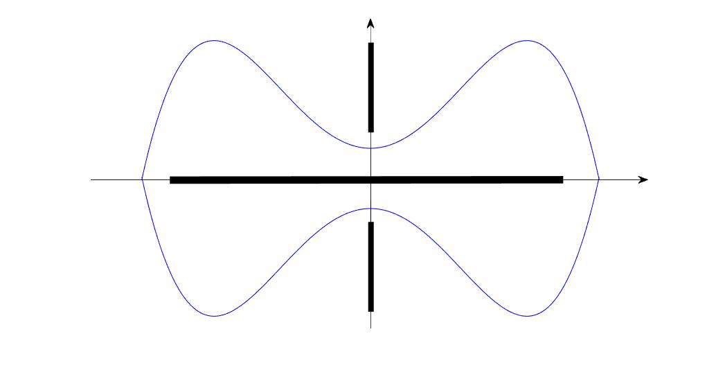
Figure 2.1: A schematic plot of the dumbbell-shaped Cauchy contour $\mathscr{C}$.

It is already clear from (2.33) that the locality of the resolvents will play an important role in our analysis. Hence, we prove a decay estimate in the next lemma.

Lemma 2.2.

Let $\mathcal{H}(y),y\in\mathcal{V}_{\mathfrak{m}}^{N}$ be a tight binding Hamiltonian of the form (2.3) and $\mathscr{C}$ a contour satisfying (2.31). If L and H.tb are satisfied, then there exist constants $\gamma_{\rm r}>0$ and $c_{\rm r}$, independent of $y$ or $N$, such that

$$\Big{(}\mathscr{R}_{z}({y})\Big{)}_{\ell k}\leq c_{\rm r}e^{-\gamma_{\rm r}|y(\ell)-y(k)|}\quad\forall~{}z\in\mathscr{C}.$$ (2.34)

Proof.

This proof relies on the arguments provided by [24] and a Combes–Thomas type estimate [20].

For $k_{0}$ and $\gamma_{\rm r}>0$, let $B\in\mathbb{R}^{\Lambda_{N}\times\Lambda_{N}}$,

$$B_{\ell k}=\left\{\begin{array}[]{ll}e^{\gamma_{\rm r}|y(\ell)-y(k_{0})|},&{\rm if}~{}\ell=k;\\[4.30554pt] 0,&{\rm otherwise}.\end{array}\right.$$ (2.37)

From this definition, we have

$$\big{[}B\mathcal{H}B^{-1}-\mathcal{H}\big{]}_{\ell k} =e^{\gamma_{\rm r}|y(\ell)-y(k_{0})|}\mathcal{H}_{\ell k}e^{-\gamma_{\rm r}|y(k)-y(k_{0})|}-\mathcal{H}_{\ell k}$$

$$=\mathcal{H}_{\ell k}\big{(}e^{\gamma_{\rm r}(|y(\ell)-y(k_{0})|-|y(k)-y(k_{0})|)}-1\big{)}.$$

Assumptions L and H.tb yield

$$\big{\|}B\mathcal{H}B^{-1}-\mathcal{H}\big{\|}_{\infty}~{}\leq~{}\sup_{\ell\in\Lambda_{N}}\sum_{k\in\Lambda_{N}}|\mathcal{H}_{\ell k}|\Big{(}e^{\gamma_{\rm r}|y(\ell)-y(k)|}-1\Big{)}$$ (2.38)

$$\leq \bar{h}_{0}\sup_{\ell\in\Lambda_{N}}\left(\bigg{(}\sum_{\begin{subarray}{c}k\in\Lambda_{N},\\ |y(\ell)-y(k)|>R\end{subarray}}e^{-(\gamma_{0}-\gamma_{\rm r})|y(\ell)-y(k)|}\bigg{)}+\bigg{(}\sum_{\begin{subarray}{c}k\in\Lambda_{N},\\ |y(\ell)-y(k)|\leq R\end{subarray}}e^{-\gamma_{0}|y(\ell)-y(k)|}\bigg{)}\big{(}e^{\gamma_{\rm r}R}-1\big{)}\right)$$

$$\leq C\Big{(}e^{-\frac{1}{2}(\gamma_{0}-\gamma_{\rm r})R}+e^{\gamma_{\rm r}R}-1\Big{)}$$

for any $\gamma_{\rm r}<\gamma_{0}/2$ and $R>0$, where $C$ is a constant depending only on $\bar{h}_{0}$, $d$, $\gamma_{0}$, $\gamma_{\rm r}$, and $\mathfrak{m}$. For any $\varepsilon>0$, we can choose $R$ sufficiently large and then $\gamma_{\rm r}$ sufficiently small (depending on $R$) such that $\|B\mathcal{H}B^{-1}-\mathcal{H}\|_{\infty}<\varepsilon$. We note that the choice of $R$ and $\gamma_{\rm r}$ does not depend on the system size $N$ but only on $\varepsilon$ and the constants $\bar{h}_{0},~{}\gamma_{0},~{}\mathfrak{m}$. Similarly, we have the same bound for $\|B\mathcal{H}B^{-1}-\mathcal{H}\|_{1}$. Using interpolation, we get the same bound for $\|B\mathcal{H}B^{-1}-\mathcal{H}\|_{2}$.

Note that

$$B(z-\mathcal{H})^{-1}B^{-1} = (z-B\mathcal{H}B^{-1})^{-1}$$

$$= (z-H)^{-1}(I-(B\mathcal{H}B^{-1}-\mathcal{H})(z-\mathcal{H})^{-1})^{-1}.$$

Since (2.31) implies $\|(z-\mathcal{H})^{-1}\|_{\mathscr{L}(l^{2})}]\leq 1/\mathfrak{d}$, we can choose $R$ and $\gamma_{\rm r}$ such that $z-B\mathcal{H}B^{-1}$ is invertible and

$$\|B(z-\mathcal{H})^{-1}B^{-1}\|_{\mathscr{L}(l^{2})}\leq\frac{2}{\mathfrak{d}}.$$

Using $\big{|}[B(z-\mathcal{H})^{-1}B^{-1}]_{\ell k}\big{|}\leq\|B(z-\mathcal{H})^{-1}B^{-1}\|_{\mathscr{L}(l^{2})}\leq 2/\mathfrak{d}$ and

$$\Big{|}\big{[}(z-\mathcal{H})^{-1}\big{]}_{\ell k}e^{\gamma_{\rm r}(|y(\ell)-y(k_{0})|-|y(k)-y(k_{0})|)}\Big{|}=\Big{|}\big{[}B(z-\mathcal{H})^{-1}B^{-1}\big{]}_{\ell k}\Big{|}\leq\frac{2}{\mathfrak{d}},$$

and consequently,

$$\left|\big{[}(z-\mathcal{H})^{-1}\big{]}_{\ell k}\right|\leq\frac{2}{\mathfrak{d}}e^{-\gamma_{\rm r}(|y(\ell)-y(k_{0})|-|y(k)-y(k_{0})|)}.$$ (2.40)

Taking $k_{0}=k$, we obtain the stated exponential decay estimate. ∎

2.3 Site energy

Since the tight binding Hamiltonian (2.1) is given in terms of an atomic-like basis set, we can distribute the energy among atomic sites. This is a well-known idea, which has been used for constructing interatomic potentials based on the bond-order concept (see e.g. [28, 29, 55]).

Noting that $\|\psi_{s}\|_{\ell^{2}}=1$ for all $s$, we have

$$E(y) =\sum_{s=1}^{N}f(\varepsilon_{s})\varepsilon_{s}=\sum_{s=1}^{N}f(\varepsilon_{s})\varepsilon_{s}\sum_{\ell\in\Lambda_{N}}[\psi_{s}]_{\ell}^{2}=\sum_{\ell\in\Lambda_{N}}\sum_{s=1}^{N}f(\varepsilon_{s})\varepsilon_{s}[\psi_{s}]_{\ell}^{2}.$$

That is, we have obtained the decomposition of the band energy

$$E(y) =\sum_{\ell\in\Lambda_{N}}E_{\ell}(y),\qquad\text{where}$$ (2.41)

$$E_{\ell}(y) =\sum_{s}f(\varepsilon_{s})\varepsilon_{s}[\psi_{s}]_{\ell}^{2}=\sum_{s}\mathfrak{f}(\varepsilon_{s})[\psi_{s}]_{\ell}^{2},$$ (2.42)

and we call $E_{\ell}(y)$ the site energy.

When the atomic orbitals are not orthogonal we slightly modify the definition of site energy slightly for computational efficiency; see Appendix B for detailed discussions.

Such a decomposition is useful, for example, since classical interatomic potentials almost always decompose the total energy in such a way, hence the relation (2.41) can be used to establish a bridge between ab initio models and empirical interaction laws [28]. For our own purpose, the decomposition will (1) yield a relatively straightforward thermodynamic limit argument to define and analyze variational problems on the infinite lattice along the lines of [27], and (2) provide a starting point for the construction and analysis of concurrent multi-scale schemes hybrid models, which we will pursue in two companion papers [18, 19].

Our aim, next, is to establish locality of $E_{\ell}$. From now on, for the sake of readability, we drop the argument $(y)$ in $\mathscr{R}_{z}({y})$, $\mathcal{H}(y)$, $\mathcal{H}_{,m}(y)$ and $\mathcal{H}_{,mn}(y)$ whenever convenient and possible without confusion and in addition write $r_{mn}=|y(m)-y(n)|$. Let $e_{\ell}$ be the $N$ dimensional canonical basis vector, then we obtain from (2.23) that

$$E_{\ell}(y) =\sum_{s}\mathfrak{f}(\varepsilon_{s})\left|[\psi_{s}]_{\ell}\right|^{2}=\sum_{s}\mathfrak{f}(\varepsilon_{s})(\psi_{s},e_{\ell})(\psi_{s},e_{\ell})=\sum_{s}\Big{(}\mathfrak{f}\big{(}\mathcal{H}\big{)}\psi_{s},e_{\ell}\Big{)}(\psi_{s},e_{\ell})$$

$$=\sum_{s}(\psi_{s},e_{\ell})\Big{(}\psi_{s},\mathfrak{f}\big{(}\mathcal{H}\big{)}e_{\ell}\Big{)}=\Big{(}e_{\ell},\mathfrak{f}\big{(}\mathcal{H}\big{)}e_{\ell}\Big{)},$$

and employing (2.32) we arrive at

$$E_{\ell}(y)=-\frac{1}{2\pi i}\oint_{\mathscr{C}}\mathfrak{f}(z)\big{[}\mathscr{R}_{z}\big{]}_{\ell\ell}~{}{\rm d}z.$$ (2.43)

We can now calculate the first and second derivatives of $E_{\ell}(y)$ based on (2.43) and the regularity assumption in H.loc:

$$\frac{\partial E_{\ell}(y)}{\partial[y(m)]_{i}} =\frac{1}{2\pi i}\oint_{\mathscr{C}}\mathfrak{f}(z)\Big{[}\mathscr{R}_{z}\left[\mathcal{H}_{,m}\right]_{i}\mathscr{R}_{z}\Big{]}_{\ell\ell}~{}{\rm d}z,\quad\text{and}$$ (2.44)

$$\frac{\partial^{2}E_{\ell}(y)}{\partial[y(m)]_{i}\partial[y(n)]_{j}} =\frac{1}{2\pi i}\oint_{\mathscr{C}}\mathfrak{f}(z)\bigg{[}\mathscr{R}_{z}\big{[}\mathcal{H}_{,mn}\big{]}_{ij}\mathscr{R}_{z}-\mathscr{R}_{z}\left[\mathcal{H}_{,m}\right]_{i}\mathscr{R}_{z}\big{[}\mathcal{H}_{,n}\big{]}_{j}\mathscr{R}_{z}$$

$$\hskip 130.0002pt-\mathscr{R}_{z}\left[\mathcal{H}_{,n}\right]_{j}\mathscr{R}_{z}\big{[}\mathcal{H}_{,m}\big{]}_{i}\mathscr{R}_{z}\bigg{]}_{\ell\ell}~{}{\rm d}z.$$ (2.45)

We also have higher order derivatives of the site energy for $n\leq\mathfrak{n}$:

$$\frac{\partial^{n}E_{\ell}(y)}{\partial[y(m_{1})]_{i_{1}}\cdots\partial[y(m_{n})]_{i_{n}}}=-\frac{1}{2\pi i}\oint_{\mathscr{C}}\mathfrak{f}(z)\Bigg{[}\sum_{l=1}^{n}\sum_{j_{1}+\cdots+j_{l}=n}\sum_{\mathcal{P}_{m_{1},\cdots,m_{n}}^{j_{1},\cdots,j_{l}}}(-1)^{l}\\[4.30554pt] Q^{(l)}_{z}[y]\Big{(}[\mathcal{H}_{,\mathcal{P}m_{1}\cdots\mathcal{P}m_{j_{1}}}(y)]_{\mathcal{P}i_{1}\cdots\mathcal{P}i_{j_{1}}},\cdots,[\mathcal{H}_{,\mathcal{P}m_{n-j_{l}+1}\cdots\mathcal{P}m_{n}}(y)]_{\mathcal{P}i_{n-j_{l}+1}\cdots\mathcal{P}i_{n}}\Big{)}\Bigg{]}_{\ell\ell}~{}{\rm d}z,\quad$$ (2.46)

where $Q^{(n)}_{z}:\left(\mathbb{R}^{N\times N}\right)^{n}\mapsto\mathbb{R}^{N\times N}$:

$$Q^{(n)}_{z}[y](\Theta_{1},\cdots,\Theta_{n})=\mathscr{R}_{z}({y})\prod_{j=1}^{n}\Big{(}\Theta_{j}\mathscr{R}_{z}({y})\Big{)}$$ (2.47)

is a well-defined linear map for any $z$ satisfying (2.31) and $\mathcal{P}_{m_{1},\cdots,m_{n}}^{j_{1},\cdots,j_{l}}$ is the multiset permutation of $m_{1},\cdots,m_{n}$.

2.4 Properties of the site energy

In order for $E_{\ell}$ to be a “true” site energy it must satisfy certain properties: locality, permutation invariance and isometry invariance. We establish these next.

First, we establish the locality of the site energy and its derivatives. We remark that in this result it is important that we are keeping $\mu$ fixed. Admitting $y$-dependent $\mu$ would introduce a small amount of non-locality in the site-energies, but it is reasonable to expect that this vanishes in the thermodynamic limit.

Lemma 2.3 (Locality).

If L, H.tb, H.loc, F are satisfied then, for $1\leq j\leq\mathfrak{n}$, there exist positive constants $C_{j}$ and $\eta_{j}$ such that for any $\ell\in\Lambda_{N}$,

$$\left|\frac{\partial^{j}E_{\ell}(y)}{\partial[y(m_{1})]_{i_{1}}\cdots\partial[y(m_{j})]_{i_{j}}}\right|\leq C_{j}e^{-\eta_{j}\sum_{l=1}^{j}|y(\ell)-y(m_{l})|}\qquad 1\leq i_{1},\cdots,i_{j}\leq d.$$ (2.48)

Proof.

We will only give the explicit proofs for $j=1,2$, the cases $j>2$ being analogous (but tedious).

For $j=1$, we have from Lemma 2.2 and the assumptions L, H.loc that

$$\Big{[}\mathscr{R}_{z}\left[\mathcal{H}_{,m}\right]_{i}\mathscr{R}_{z}\Big{]}_{\ell\ell} =\sum_{\ell_{1},\ell_{2}\in\Lambda_{N}}\big{[}\mathscr{R}_{z}\big{]}_{\ell\ell_{1}}\big{(}\left[\mathcal{H}_{,m}\right]_{i}\big{)}_{\ell_{1}\ell_{2}}\big{[}\mathscr{R}_{z}\big{]}_{\ell_{2}\ell}$$

$$\leq c_{\rm r}^{2}\bar{h}_{1}\sum_{\ell_{1},\ell_{2}\in\Lambda_{N}}e^{-\min\{\gamma_{\rm r},\gamma_{1}\}\big{(}r_{\ell\ell_{1}}+r_{\ell_{1}m}+r_{m\ell_{2}}+r_{\ell_{2}\ell}\big{)}}$$

$$=c_{\rm r}^{2}\bar{h}_{1}\bigg{(}\sum_{\ell_{1}\in\Lambda_{N}}e^{-\min\{\gamma_{\rm r},\gamma_{1}\}\big{(}r_{\ell\ell_{1}}+r_{\ell_{1}m}\big{)}}\bigg{)}^{2}$$

$$\leq Ce^{-\min\{\gamma_{\rm r},\gamma_{1}\}|y(\ell)-y(m)|},\qquad\quad$$ (2.49)

where $C$ depends only on $\bar{h}_{1},c_{\rm r},\gamma_{\rm r},\gamma_{1},\mathfrak{m}$ and $d$. Together with (2.44) and F, this leads to

$$\frac{\partial E_{\ell}(y)}{\partial[y(m)]_{i}}\leq C_{1}e^{-\eta_{1}|y(\ell)-y(m)|}\quad{\rm for}~{}1\leq i\leq d.$$ (2.50)

For $j=2$, we employ Lemma 2.2 and L, H.loc to estimate the three term arising in the expression (2.45) of the site Hessian, using similar computations as (2.49):

$$\Big{[}\mathscr{R}_{z}\left[\mathcal{H}_{,m}\right]_{i}\mathscr{R}_{z}\left[\mathcal{H}_{,n}\right]_{j}\mathscr{R}_{z}\Big{]}_{\ell\ell}$$

$$\leq c_{\rm r}^{3}\bar{h}_{1}^{2}\sum_{\ell_{1},\ell_{2},\ell_{3},\ell_{4}\in\Lambda_{N}}e^{-\min\{\gamma_{\rm r},\gamma_{1}\}\big{(}r_{\ell\ell_{1}}+r_{\ell_{1}m}+r_{\ell_{2}m}+r_{\ell_{2}\ell_{3}}+r_{\ell_{3}n}+r_{\ell_{4}n}+r_{\ell_{4}\ell}\big{)}}$$

$$\leq Ce^{-\frac{1}{2}\min\{\gamma_{\rm r},\gamma_{1}\}(|y(\ell)-y(m)|+|y(\ell)-y(n)|)};$$

$$\Big{[}\mathscr{R}_{z}\left[\mathcal{H}_{,n}\right]_{j}\mathscr{R}_{z}\left[\mathcal{H}_{,m}\right]_{i}\mathscr{R}_{z}\Big{]}_{\ell\ell}$$

$$\leq Ce^{-\frac{1}{2}\min\{\gamma_{\rm r},\gamma_{1}\}(|y(\ell)-y(m)|+|y(\ell)-y(n)|)};\qquad\text{and}$$

$$\Big{[}\mathscr{R}_{z}\left[\mathcal{H}_{,mn}\right]_{ij}\mathscr{R}_{z}\Big{]}_{\ell\ell}$$

$$\leq c_{\rm r}^{2}\bar{h}_{2}\sum_{\ell_{1},\ell_{2}\in\Lambda_{N}}e^{-\min\{\gamma_{\rm r},\gamma_{2}\}(r_{\ell\ell_{1}}+r_{\ell_{1}m}+r_{\ell_{1}n}+r_{\ell_{2}m}+r_{\ell_{2}n}+r_{\ell_{2}\ell})}$$

$$\leq Ce^{-\frac{1}{2}\min\{\gamma_{\rm r},\gamma_{2}\}(|y(\ell)-y(m)|+|y(\ell)-y(n)|)}.$$

Inserting these three estimates into (2.45) together with F yields the desired result,

$$\frac{\partial^{2}E_{\ell}(y)}{\partial[y(m)]_{i}\partial[y(n)]_{j}}\leq C_{2}e^{-\eta_{2}\big{(}|y(\ell)-y(m)|+|y(\ell)-y(n)|\big{)}}\quad{\rm for}~{}1\leq i,j\leq d.\qed$$

The next lemma summarises the consequences of H.sym.

Lemma 2.4 (Symmetries).

Let $y\in\mathcal{V}^{N}_{\mathfrak{m}}$. Assume that H.sym is satisfied.

• (Isometry invariance) if $g:\mathbb{R}^{d}\rightarrow\mathbb{R}^{d}$ is an isometry, then $E_{\ell}(y)=E_{\ell}(g(y))$;

• (Permutation invariance) if $\mathcal{G}:\Lambda\rightarrow\Lambda$ is a permutation (relabelling) of $\Lambda$, then $E_{\ell}(y)=E_{\mathcal{G}^{-1}(\ell)}(y\circ\mathcal{G})$.

Proof.

(i) Let $y^{\prime}=g(y)$. Since $g$ is an isometry, we have that $y^{\prime}\in\mathcal{V}^{N}_{\mathfrak{m}}$. The assumption H.sym (i) implies $h_{mn}(y)=h_{mn}(y^{\prime})$, which together with (2.43) yields

$$E_{\ell}(y)=-\frac{1}{2\pi i}\oint_{\mathscr{C}}\mathfrak{f}(z)\left[\mathscr{R}_{z}({y})\right]_{\ell\ell}~{}{\rm d}z=-\frac{1}{2\pi i}\oint_{\mathscr{C}}\mathfrak{f}(z)\left[\mathscr{R}_{z}({y^{\prime}})\right]_{\ell\ell}~{}{\rm d}z=E_{\ell}(y^{\prime}).$$ (2.51)

(ii) Let $y^{\prime}=y\circ\mathcal{G}$. The assumption H.sym (ii) implies $h_{mn}(y)=h_{\mathcal{G}^{-1}(m)\mathcal{G}^{-1}(n)}(y^{\prime})$, which together with (2.43) leads to $E_{\ell}(y)=E_{\mathcal{G}^{-1}(\ell)}(y^{\prime})$. ∎

3 Pointwise thermodynamic limit

Our aim in this section is to give a meaning to energy in the infinite body limit (“thermodynamic limit”). The notion of site energy makes this relatively straightforward: we will prove that, fixing a site $\ell$, and “growing” the material around it to an infinite body yields a well-defined site energy functional $E_{\ell}$ for an infinite body. Total energy in an infinite body is of course ill-defined, but using the site energies it then becomes straightforward to consider energy-differences; cf. § 4.

We need the following additional assumption, connecting the Hamiltonians for growing index-sets, in our analysis.

H.emb. Let $y^{N}:\Lambda_{N}\rightarrow\mathbb{R}^{d}$, $y:\Lambda_{N}\cup\{x^{\prime}\}\rightarrow\mathbb{R}^{d}$ be two configurations satisfying L, and $h^{N}_{\ell k}(y^{N})$, $h_{\ell k}(y)$ be the corresponding Hamiltonian matrix elements of these two configurations satisfying H.loc. If $y^{N}(\ell)=y(\ell)$ for any $\ell\in\Lambda_{N}$, then for $0\leq j\leq\mathfrak{n}-1$,

$$\frac{\partial^{j}h^{N}_{\ell k}(y^{N})}{\partial[y(m_{1})]_{i_{1}}\cdots\partial[y(m_{j})]_{i_{j}}}=\lim_{|y(x^{\prime})|\rightarrow\infty}\frac{\partial^{j}h_{\ell k}(y)}{\partial[y(m_{1})]_{i_{1}}\cdots\partial[y(m_{j})]_{i_{j}}}\quad\forall~{}\ell,k\in\Lambda_{N}$$ (3.1)

with $m_{1},\cdots,m_{j}\in\Lambda_{N}$ and $1\leq i_{1},\cdots,i_{j}\leq d$.

Remark 3.1.

Intuitively, H.emb states that, if one atom $y(x^{\prime})$ in the system is moved to infinity, then the Hamiltonian matrix elements for the remaining subsystem $\{y(\ell)~{}\lvert~{}\ell\in\Lambda_{N}\}$ do not depend on $y(x^{\prime})$ anymore.

At first glance, this appears to be a consequence of H.tb and H.loc. The reason we have to formulate it as a separate assumption is to make a connection between the Hamiltonians for $\Lambda_{N}$ and $\Lambda_{N}\cup\{x^{\prime}\}$. More generally, in Lemma 3.1, we obtain an analogous connection between the Hamiltonians for any two systems $\Lambda_{N},\Lambda_{M}$ with $\Lambda_{N}\subset\Lambda_{M}$.

Let $\Lambda$ be a countable index set (or, reference configuration), then we consider deformed configurations belonging to the class

$$\mathcal{V}_{\mathfrak{m}}(\Lambda) := \left\{y:\Lambda\rightarrow\mathbb{R}^{d},~{}~{}y|_{\Lambda_{N}}\subset\mathcal{V}_{\mathfrak{m}}^{N}~{}~{}{\rm for~{}any~{}finite~{}}\Lambda_{N}\subset\Lambda\right\}$$ (3.2)

$$= \big{\{}y:\Lambda\to\mathbb{R}^{d},|y(\ell)-y(k)|\geq\mathfrak{m}\text{ for all }\ell,k\in\Lambda\big{\}}.$$

If $y\in\mathcal{V}_{\mathfrak{m}}(\Lambda)$, then L is satisfied for any finite subsystem $\Lambda_{N}\subset\Lambda$. In the following, whenever we assume H.tb, H.loc and H.emb for infinite $\Lambda$, we mean that they are satisfied for the Hamiltonian matrices of any finite subsystem $\Lambda_{N}\subset\Lambda$.

For a bounded domain $\Omega\subset\mathbb{R}^{d}$, we shall denote the Hamiltonian, resolvent and energy of the finite subsystem contained in $\Omega$, respectively, by $\mathcal{H}^{\Omega}(y)$, $\mathscr{R}_{z}^{\Omega}({y})$ and $E^{\Omega}(y)$. For simplicity of notation, we drop the argument $(y)$ whenever convenient.

Theorem 3.1.

Let $\Lambda$ be countable and $y\in\mathcal{V}_{\mathfrak{m}}(\Lambda)$ be a deformation. Suppose the assumptions F, H.tb, H.loc, H.emb and H.sym are satisfied for all finite subsystems (with simultaneous choice of constants), then

• (existence of the thermodynamic limits) for any $\ell\in\Lambda$ and for any sequence of convex and bounded sets $\Omega_{R}\supset B_{R}(y(\ell)),R>0$ the limit

  $$E_{\ell}(y):=\lim_{R\rightarrow\infty}E^{\Omega_{R}}_{\ell}(y)$$ (3.3)

  exists and is independent of the choice of sets $\Omega_{R}$;

• (regularity and locality of the limits) the limits $E_{\ell}(y)$ possess $j$th order partial derivatives with $1\leq j\leq\mathfrak{n}-1$, and it holds that

  $$\left|\frac{\partial^{j}E_{\ell}(y)}{\partial[y(m_{1})]_{i_{1}}\cdots\partial[y(m_{j})]_{i_{j}}}\right|\leq C_{j}e^{-\eta_{j}\sum_{l=1}^{j}|y(\ell)-y(m_{l})|}\quad 1\leq i_{1},\cdots,i_{j}\leq d,$$ (3.4)

  where the constants $C_{j}$ and $\eta_{j}$ are same to those in Lemma 2.3;

• (isometry invariance) if $g:\mathbb{R}^{d}\rightarrow\mathbb{R}^{d}$ is an isometry, then $E_{\ell}(y)=E_{\ell}(g(y))$;

• (permutation invariance) if $\mathcal{G}:\Lambda\rightarrow\Lambda$ is a permutation (relabelling) of $\Lambda$, then $E_{\ell}(y)=E_{\mathcal{G}^{-1}(\ell)}(y\circ\mathcal{G})$.

Before we prove Theorem 3.1 we establish an extension of H.emb.

Lemma 3.1.

Let $\Lambda_{M}\supsetneq\Lambda_{N}$, $y^{M}:\Lambda_{M}\rightarrow\mathbb{R}^{d}$ and $y^{N}:\Lambda_{N}\rightarrow\mathbb{R}^{d}$ be two configurations satisfying L. Assume that there exists a convex set $\Omega\subset\mathbb{R}^{d}$ such that

$$y^{M}(\ell)=y^{N}(\ell)\in\Omega\quad\forall~{}\ell\in\Lambda_{N}\qquad{\rm and}\qquad y^{M}(\ell)\in\Omega^{\rm c}\quad\forall~{}\ell\in\Lambda_{M}\backslash\Lambda_{N},$$

where $\Omega^{\rm c}$ is the complement of $\Omega$ in $\mathbb{R}^{d}$. If F, H.loc, H.ext are satisfied then, for $0\leq j\leq\mathfrak{n}-1$, there exist positive constants $c_{j},\kappa_{j}$, which do not depend on $M$, $N$ and $\Omega$, such that

$$|h_{\ell k}^{M}(y^{M})-h_{\ell k}^{N}(y^{N})|\leq c_{0}\exp\Big{(}-\kappa_{0}\Big{(}{\rm dist}\left(y^{N}(\ell),\Omega^{\rm c}\right)+{\rm dist}\left(y^{N}(k),\Omega^{\rm c}\right)\Big{)}\Big{)},$$ (3.5)

and

$$\left|\frac{\partial^{j}h^{M}_{\ell k}(y^{M})}{\partial[y(m_{1})]_{i_{1}}\cdots\partial[y(m_{j})]_{i_{j}}}-\frac{\partial^{j}h^{N}_{\ell k}(y^{N})}{\partial[y(m_{1})]_{i_{1}}\cdots\partial[y(m_{j})]_{i_{j}}}\right|$$

$$\leq c_{j}\exp\Big{(}-\kappa_{j}\Big{(}{\rm dist}\left(y^{N}(\ell),\Omega^{\rm c}\right)+{\rm dist}\left(y^{N}(k),\Omega^{\rm c}\right)$$

$$\hskip 140.00021pt+\sum_{s=1}^{j}(|y^{N}(\ell)-y^{N}(m_{s})|+|y^{N}(k)-y^{N}(m_{s})|)\Big{)}\Big{)}$$

for any $\ell,k,m_{s}\in\Lambda_{N}$ and $1\leq i_{1},\dots,i_{j}\leq d$.

Proof.

We first prove the case $j=0$, i.e., (3.5). For each $\ell\in\Lambda_{M}\backslash\Lambda_{N}$, we can find a normalized vector $\nu_{\ell}$ such that $y^{M}(\ell)-\nu_{\ell}\cdot{\rm dist}\left(y^{M}(\ell),\Omega\right)\in\overline{\Omega}$. Let $\{R^{\mu}_{\ell}\}_{\mu\in\mathbb{N}}$ be a sequence for each $\ell\in\Lambda_{M}\backslash\Lambda_{N}$, such that $R^{\mu}_{\ell}\rightarrow\infty$ as $\mu\rightarrow\infty$, then we define

$$\tilde{y}^{\mu}(\ell):=\left\{\begin{array}[]{ll}y^{N}(\ell)&{\rm if}~{}\ell\in\Lambda_{N};\\[4.30554pt] y^{M}(\ell)+{\nu}_{\ell}\cdot R^{\mu}_{\ell}&{\rm if}~{}\ell\in\Lambda_{M}\backslash\Lambda_{N}.\end{array}\right.$$

Using H.emb with $j=0$ and an elementary argument we can inductively choose $R_{\ell}^{\mu}$, such that $R^{\mu}:=\min_{\ell\in\Lambda_{M}\backslash\Lambda_{N}}R^{\mu}_{\ell}\rightarrow\infty$ as $\mu\rightarrow\infty$ and

$$h_{\ell k}^{N}(y^{N})=\lim_{\mu\rightarrow\infty}h_{\ell k}^{M}(\tilde{y}^{\mu}).$$ (3.8)

Note that the convexity of $\Omega$ implies

$$|y^{M}(\ell)-y^{M}(n)+c\nu_{n}|\geq\frac{1}{2}\Big{(}|y^{M}(\ell)-y^{M}(n)|+c\Big{)}$$

for any $n\in M\backslash N$ and $c>0$. Using the assumptions L and H.loc with $j=1$, we have

$$\big{|}h_{\ell k}^{M}(\tilde{y}^{\mu})-h_{\ell k}^{M}(y^{M})\big{|}~{}=~{}\left|\int_{0}^{1}\sum_{n\in\Lambda_{M}\setminus\Lambda_{N}}\frac{\partial h_{\ell k}^{M}}{\partial y(n)}\Big{(}(1-t)y^{M}+t\tilde{y}^{\mu}\Big{)}\cdot\big{(}\tilde{y}^{\mu}(n)-y^{M}(n)\big{)}~{}{\rm d}t\right|$$

$$\leq C\bar{h}_{1}\int_{0}^{1}\sum_{n\in\Lambda_{M}\backslash\Lambda_{N}}e^{-\gamma_{1}\big{(}|y^{M}(\ell)-y^{M}(n)+tR^{\mu}\nu_{n}|+|y^{M}(k)-y^{M}(n)+tR^{\mu}\nu_{n}|\big{)}}\cdot R^{\mu}~{}{\rm d}t$$

$$\leq C\bar{h}_{1}\sum_{n\in\Lambda_{M}\backslash\Lambda_{N}}e^{-\frac{\gamma_{1}}{2}\big{(}|y^{M}(\ell)-y^{M}(n)|+|y^{M}(k)-y^{M}(n)|\big{)}}\cdot\int_{0}^{1}e^{-\gamma_{1}tR^{\mu}}R^{\mu}~{}{\rm d}t$$

$$\leq c_{0}e^{-\kappa_{0}\big{(}{\rm dist}\left(y^{N}(\ell),\Omega^{\rm c}\right)+{\rm dist}\left(y^{N}(k),\Omega^{\rm c}\right)\big{)}}\cdot\big{(}1-e^{-\gamma_{1}R^{\mu}}\big{)},$$

where $\kappa_{0}=\gamma_{1}/2-\varepsilon$ with any $\varepsilon\in(0,\gamma_{1}/2)$, and $c_{0}$ is a constant depending only on $\varepsilon$, $\bar{h}_{1}$, $\gamma_{1}$, $\mathfrak{m}$ and $d$. Note that neither $\kappa_{0}$ nor $c_{0}$ depends on the system size $M$, $N$ and $\Omega$. Note that

$$\big{|}h_{\ell k}^{M}(y^{M})-h_{\ell k}^{N}(y^{N})\big{|}=\lim_{\mu\rightarrow\infty}\big{|}h_{\ell k}^{M}(y^{M})-h_{\ell k}^{M}(\tilde{y}^{\mu})\big{|}\leq c_{0}e^{-\kappa_{0}\big{(}{\rm dist}\left(y^{N}(\ell),\Omega^{\rm c}\right)+{\rm dist}\left(y^{N}(k),\Omega^{\rm c}\right)\big{)}},$$

which completes the proof of the case $j=0$.

With the same arguments, we can prove (3.1) for $1\leq j\leq\mathfrak{n}-1$ by using the assumptions H.loc with index $j+1$ and H.emb with index $j$. ∎

Proof of Theorem 3.1.

(i) Without loss of generality, we can assume that the upper bound of the spectrum $\overline{\sigma}<0$ (one can always shift the eigenvalues if this is not satisfied) and the contour $\mathscr{C}$ is chosen such that it includes 0 and

$$\min\left\{{\rm dist}\big{(}\mathscr{C},\sigma(\mathcal{H}(y))\big{)},{\rm dist}\big{(}\mathscr{C},\mathfrak{s}(\mathfrak{f})\big{)},{\rm dist}\big{(}\mathscr{C},\{0\}\big{)}\right\}\geq\mathfrak{d}.$$ (3.9)

Let $\ell\in\Lambda$ and $B_{R}(y(\ell))\subset\Omega_{R}\subsetneq\Omega^{\prime}$, then we define

$$\Big{[}\widetilde{\mathcal{H}}^{\Omega_{R}}(y)\Big{]}_{km}:=\left\{\begin{array}[]{ll}\big{[}\mathcal{H}^{\Omega_{R}}(y)\big{]}_{km}&\text{if }y(k),y(m)\in\Omega_{R};\\[4.30554pt] 0&\text{otherwise for }y(k),y(m)\in\Omega^{\prime}.\end{array}\right.$$ (3.12)

Note that (3.9) implies that the condition (2.31) is satisfied for the Hamiltonian $\widetilde{\mathcal{H}}^{\Omega_{R}}$ with the contour $\mathscr{C}$. Moreover, the resolvent $\widetilde{\mathscr{R}}^{\Omega_{R}}_{z}(y)=(\widetilde{\mathcal{H}}^{\Omega_{R}}(y)-zI)^{-1}$ is well-defined for any $z\in\mathscr{C}$ and satisfies the estimate in (2.34). Under the assumption F, we can observe that the band energy and site energies of the Hamiltonian $\mathcal{H}^{\Omega_{R}}(y)$ and $\widetilde{\mathcal{H}}^{\Omega_{R}}(y)$ are the same.

We have from (2.43), (3.12), L, H.tb, Lemma 3.1 and Lemma 2.2 that

$$E^{\Omega^{\prime}}_{\ell}(y)-E^{\Omega_{R}}_{\ell}(y)~{}=~{}-\frac{1}{2\pi i}\oint_{\mathscr{C}}\mathfrak{f}(z)\Big{[}\mathscr{R}_{z}^{\Omega^{\prime}}-\widetilde{\mathscr{R}}_{z}^{\Omega_{R}}\Big{]}_{\ell\ell}~{}{\rm d}z$$

$$\leq C\sum_{y(\ell_{1}),y(\ell_{2})\in\Omega^{\prime}}\big{[}\mathscr{R}_{z}^{\Omega^{\prime}}\big{]}_{\ell\ell_{1}}\big{[}\mathcal{H}^{\Omega^{\prime}}-\widetilde{\mathcal{H}}^{\Omega_{R}}\big{]}_{\ell_{1}\ell_{2}}[\widetilde{\mathscr{R}}_{z}^{\Omega_{R}}]_{\ell_{2}\ell}$$

$$\leq C\sum_{y(\ell_{1}),y(\ell_{2})\in\Omega^{\prime}}e^{-\gamma_{\bf r}r_{\ell\ell_{1}}}e^{-\kappa_{0}\big{(}{\rm dist}\left(y(\ell_{1}),\Omega^{\prime}\backslash\Omega_{R}\right)+{\rm dist}\left(y(\ell_{2}),\Omega^{\prime}\backslash\Omega_{R}\right)\big{)}}e^{-\gamma_{\bf r}r_{\ell\ell_{2}}}$$

$$\leq C\left(\sum_{y(\ell_{1})\in\Omega^{\prime}}e^{-\gamma_{\bf r}r_{\ell\ell_{1}}-\kappa_{0}{\rm dist}\left(y(\ell_{1}),\Omega^{\prime}\backslash\Omega_{R}\right)}\right)^{2}~{}\leq~{}Ce^{-\min\{\gamma_{\bf r},\kappa_{0}\}R},$$ (3.13)

where the last constant $C$ depends only on $\bar{h}_{0}$, $c_{\rm r}$, $c_{0}$, $\gamma_{\bf r}$, $\kappa_{0}$, $\mathfrak{m}$ and $d$, but is independent of $y$ or $R$. Since (3.13) holds for any $\Omega^{\prime}\supsetneq B_{R}(y(\ell))$ it follows that $\left\{E^{\Omega_{R}}_{\ell}(y)\right\}_{R\in\mathbb{N}}$ is a Cauchy sequence. The uniqueness of the limit is also an immediate consequence of the fact that $\Omega^{\prime}$ was arbitrary. This completes the proof of (i).

(ii) Case $j=1$:

For $\ell,m\in\Lambda$, we take $R>2|y(m)-y(\ell)|$, and then adopt the notation in the proof of (i). With the expression of (2.44), we obtain by a direct calculation that

$$\frac{\partial E^{\Omega^{\prime}}_{\ell}(y)}{\partial[y(m)]_{i}}-\frac{\partial E^{\Omega_{R}}_{\ell}(y)}{\partial[y(m)]_{i}}=\frac{1}{2\pi i}\oint_{\mathscr{C}}\mathfrak{f}(z)\Bigg{[}\widetilde{\mathscr{R}}^{\Omega_{R}}_{z}\left(\widetilde{\mathcal{H}}^{\Omega_{R}}-\mathcal{H}^{\Omega^{\prime}}\right)\mathscr{R}^{\Omega^{\prime}}_{z}\big{[}\widetilde{\mathcal{H}}^{\Omega_{R}}_{,m}\big{]}_{i}\mathscr{R}^{\Omega^{\prime}}_{z}+\\[4.30554pt] \widetilde{\mathscr{R}}^{\Omega_{R}}_{z}\big{[}\mathcal{H}^{\Omega^{\prime}}_{,m}\big{]}_{i}\mathscr{R}^{\Omega^{\prime}}_{z}\left(\widetilde{\mathcal{H}}^{\Omega_{R}}-\mathcal{H}^{\Omega^{\prime}}\right)\widetilde{\mathscr{R}}^{\Omega_{R}}_{z}+\widetilde{\mathscr{R}}^{\Omega_{R}}_{z}\left(\big{[}\mathcal{H}^{\Omega^{\prime}}_{,m}\big{]}_{i}-\big{[}\widetilde{\mathcal{H}}^{\Omega_{R}}_{,m}\big{]}_{i}\right)\widetilde{\mathscr{R}}^{\Omega_{R}}_{z}\Bigg{]}_{\ell\ell}~{}{\rm d}z.$$ (3.14)

Using L, H.tb, Lemma 3.1 and Lemma 2.2, we can obtain from a similar argument as in (3.13) that

$$\left|\frac{\partial E^{\Omega^{\prime}}_{\ell}(y)}{\partial[y(m)]_{i}}-\frac{\partial E^{\Omega_{R}}_{\ell}(y)}{\partial[y(m)]_{i}}\right|\leq Ce^{-\min\{\gamma_{\bf r},\kappa_{0},\kappa_{1}\}\big{(}R+|y(\ell)-y(m)|\big{)}/2},$$ (3.15)

where the constant $C$ depends only on $\bar{h}_{0},c_{\rm r}$, $c_{0}$, $c_{1}$, $\gamma_{\bf r}$, $\kappa_{0}$, $\kappa_{1}$, $\mathfrak{m}$ and $d$. Note that the estimate in (3.15) can be bounded by $Ce^{-\min\{\gamma_{\bf r},\kappa_{0},\kappa_{1}\}R/2}$, which does not depend on $y$. Therefore, we have that $\left\{\partial E^{R}_{\ell}(y)/\partial[y(m)]_{i}\right\}_{R\in\mathbb{N}}$ converge uniformly to some limit, which together with (i) implies that $E_{\ell}(y)$ is differentiable with respect to $y(m)$ and the derivative is given by

$$\frac{\partial E_{\ell}(y)}{\partial[y(m)]_{i}}=\lim_{R\rightarrow\infty}\frac{\partial E^{B_{R}(y(\ell))}_{\ell}(y)}{\partial[y(m)]_{i}}\quad~{}{\rm for}~{}1\leq i\leq d.$$ (3.16)

Case $j>1$:

For the second order derivatives, we can obtain from the expression (2.45) and a tedious calculation that

$$\frac{\partial^{2}E^{\Omega^{\prime}}_{\ell}(y)}{\partial[y(m)]_{i}\partial[y(n)]_{j}}-\frac{\partial^{2}E^{\Omega_{R}}_{\ell}(y)}{\partial[y(m)]_{i}\partial[y(n)]_{j}}$$

$$=~{} \frac{1}{2\pi i}\oint_{\mathscr{C}}\mathfrak{f}(z)\Bigg{[}\Bigg{.}\widetilde{\mathscr{R}}^{\Omega_{R}}_{z}\left(\mathcal{H}^{\Omega^{\prime}}-\widetilde{\mathcal{H}}^{\Omega_{R}}\right)\mathscr{R}^{\Omega^{\prime}}_{z}\big{[}\widetilde{\mathcal{H}}^{\Omega_{R}}_{,m}\big{]}_{i}\widetilde{\mathscr{R}}^{\Omega_{R}}_{z}\big{[}\mathcal{H}^{\Omega^{\prime}}_{,n}\big{]}_{j}\widetilde{\mathscr{R}}^{\Omega_{R}}_{z}$$

$$+\mathscr{R}^{\Omega^{\prime}}_{z}\left(\big{[}\widetilde{\mathcal{H}}_{,m}^{\Omega_{R}}\big{]}_{i}-\big{[}\mathcal{H}_{,m}^{\Omega^{\prime}}\big{]}_{i}\right)\widetilde{\mathscr{R}}^{\Omega_{R}}_{z}\big{[}\widetilde{\mathcal{H}}^{\Omega_{R}}_{,n}\big{]}_{j}\mathscr{R}^{\Omega^{\prime}}_{z}$$

$$+\widetilde{\mathscr{R}}^{\Omega_{R}}_{z}\left(\widetilde{\mathcal{H}}^{\Omega_{R}}-\mathcal{H}^{\Omega^{\prime}}\right)\mathscr{R}^{\Omega^{\prime}}_{z}\big{[}\widetilde{\mathcal{H}}^{\Omega_{R}}_{,mn}\big{]}_{ij}\mathscr{R}^{\Omega^{\prime}}_{z}$$

$$+\widetilde{\mathscr{R}}^{\Omega_{R}}_{z}\left(\big{[}\mathcal{H}^{\Omega^{\prime}}_{,mn}\big{]}_{ij}-\big{[}\widetilde{\mathcal{H}}^{\Omega_{R}}_{,mn}\big{]}_{ij}\right)\widetilde{\mathscr{R}}^{\Omega_{R}}_{z}+\cdots\Bigg{.}\Bigg{]}_{\ell\ell}~{}{\rm d}z.\qquad$$

For readability, we have omitted eight other terms in the square bracket, which have the same structure as the listed four terms. By estimating each term using the same arguments in (3.13), we can obtain

$$\left|\frac{\partial^{2}E^{\Omega^{\prime}}_{\ell}(y)}{\partial[y(m)]_{i}\partial[y(n)]_{j}}-\frac{\partial^{2}E^{\Omega_{R}}_{\ell}(y)}{\partial[y(m)]_{i}\partial[y(n)]_{j}}\right|\leq Ce^{-\min\{\gamma_{\bf r},\kappa_{0},\kappa_{1},\kappa_{2}\}\big{(}R+r_{\ell m}+r_{\ell n}\big{)}/4},~{}~{}$$ (3.17)

which leads to the existence of $\partial^{2}E_{\ell}(y)/\partial[y(m)]_{i}\partial[y(n)]_{j}$ and

$$\frac{\partial^{2}E_{\ell}(y)}{\partial[y(m)]_{i}\partial[y(n)]_{j}}=\lim_{R\rightarrow\infty}\frac{\partial^{2}E^{\Omega_{R}}_{\ell}(y)}{\partial[y(m)]_{i}\partial[y(n)]_{j}}\quad~{}{\rm for}~{}1\leq i,j\leq d.$$ (3.18)

For $2<j\leq\mathfrak{n}-1$, we can obtain by similar arguments that

$$\frac{\partial^{j}E_{\ell}(y)}{\partial[y(m_{1})]_{i_{1}}\cdots\partial[y(m_{j})]_{i_{j}}}=\lim_{R\rightarrow\infty}\frac{\partial^{j}E^{\Omega_{R}}_{\ell}(y)}{\partial[y(m_{1})]_{i_{1}}\cdots\partial[y(m_{j})]_{i_{j}}}\quad 1\leq i_{1},\cdots,i_{j}\leq d~{}~{}$$ (3.19)

for any sequence $\Omega_{R}$ satisfying the conditions of (i).

The locality of $E_{\ell}$ in (ii) is now an immediate consequence of Lemma 2.3 and (3.16), (3.18), (3.19).

(iii) Let $y^{\prime}=g(y)$. Since $g$ is an isometry, we have that $g\big{(}B_{R}(y(\ell))\big{)}=B_{R}(y^{\prime}(\ell))$ for any $R>0$. We can obtain from H.sym (i) and Lemma 2.4(i) that

$$E_{\ell}^{B_{R}(y(\ell))}(y)=E_{\ell}^{B_{R}(y^{\prime}(\ell))}(y^{\prime}).$$ (3.20)

Taking the limit $R\rightarrow\infty$ of (3.20) and (i) yield $E_{\ell}(y)=E_{k}(y^{\prime})$.

(iv) Similar to the proof of (iii), (iv) is a consequence of Lemma 2.4(ii) and (i). ∎

Theorem 3.1 states the existence of the thermodynamic limits of the site energies, as well as the regularity, locality and isometry/permutation invariance of the limits. In the following we shall always denote this limiting site energy by $E_{\ell}$.

Remark 3.2.

We have only considered the band energy of the system so far. The repulsive energy $E^{\rm rep}$ can be incorporated into our analysis without difficulty.

Using the expression (2.27) and the assumption U, it is easy to justify the thermodynamic limit of the repulsive site energy $E_{\ell}^{\rm rep}$, as well as its regularity and locality as those in Theorem 3.1. Moreover, the symmetry results in Theorem 3.1 are also clearly satisfied with the expression (2.27) for $E_{\ell}^{\rm rep}$. Therefore, all we have to do is to take the total site energy

$$E_{\ell}^{\rm tot}=E_{\ell}+E_{\ell}^{\rm rep}$$

and then use the existing results for $E_{\ell}$. For convenience and readability, we still work with the site band energy $E_{\ell}$ and continue to ignore the repulsive component.

4 Applications

4.1 Tight-binding model for point defects

As alluded to in the Introduction, our primary aim in understanding the locality of the TB model is the construction and rigorous analysis of QM/MM hybrid schemes for crystalline defects, along the lines of [27]. The next step towards this end is a rigorous definition of a variational problem that is to be solved. Since we have shown in Theorem 3.1 that the total TB energy can be split into exponentially localised site energies, this is a relatively straightforward generalisation of the analysis in [27], which considers MM site energies with bounded interaction radius.

Here, we only summarize the results, with an eye to the application we present in § 4.2. For simplicity we restrict ourselves to point defects only. Complete proofs and generalisations to general dislocation structures are given in [17].

We call an index set $\Lambda$ a point defect reference configuration if

D. $\exists~{}R_{\rm def}>0,A\in{\rm SL}(d)$ such that $\Lambda\backslash B_{R_{\rm def}}=(A\mathbb{Z}^{d})\backslash B_{R_{\rm def}}$ and $\Lambda\cap B_{R_{\rm def}}$ is finite.

While, in previous sections, we have worked with deformations $y$ where $y(\ell)$ denotes the deformed position of an atom indexed by $\ell$, it is now more convenient to work with displacements $u:\Lambda\to\mathbb{R}^{d}$, $u(\ell)=y(\ell)-\ell$. For displacements $u$ we define the energy-difference functional

$$\mathcal{E}(u):=\sum_{\ell\in\Lambda}\big{[}E_{\ell}(x+u)-E_{\ell}(x)\big{]},$$ (4.1)

where $x$ denotes the identity map $x:\Lambda\to\mathbb{R}^{d},x(\ell)=\ell$. Due to the exponential localisation of $E_{\ell}$ this series converges absolutely if $u$ has compact support, i.e., for $u\in\dot{\mathscr{W}^{\rm c}}$ with

$$\dot{\mathscr{W}^{\rm c}}:=\big{\{}u:\Lambda\to\mathbb{R}^{d},\exists R>0\text{ s.t. }u={\rm const}\text{ in }\Lambda\setminus B_{R}\big{\}};$$

cf. Theorem 4.1(i).

Next, still following [27], we extend the definition of $\mathcal{E}$ to a natural energy space. For $\ell\in\Lambda,\rho\in\Lambda-\ell:=\{m-\ell,m\in\Lambda\setminus\{\ell\}\}$ we define $D_{\rho}u(\ell):=u(\ell+\rho)-u(\ell)$, and moreover,

$$Du(\ell):=\big{(}D_{\rho}u(\ell)\big{)}_{\rho\in\Lambda-\ell}.$$

We think of $Du(\ell)\in(\mathbb{R}^{d})^{\Lambda-\ell}$ as an (infinite) finite-difference stencil. For any such stencil $Du(\ell)$ and $\gamma>0$ we define the norm

$$\big{|}Du(\ell)\big{|}_{\gamma}:=\bigg{(}\sum_{\rho\in\Lambda-\ell}e^{-2\gamma|\rho|}\big{|}D_{\rho}u(\ell)\big{|}^{2}\bigg{)}^{1/2},$$

which gives rise to an associated semi-norm on displacements,

$$\|Du\|_{\ell^{2}_{\gamma}}:=\bigg{(}\sum_{\ell\in\Lambda}|Du(\ell)|_{\gamma}^{2}\bigg{)}^{1/2}.$$

All (semi-)norms $\|\cdot\|_{\ell^{2}_{\gamma}},\gamma>0,$ are equivalent. With these definitions we can now define the function space, which encodes the far-field boundary condition for displacements,

$$\dot{\mathscr{W}}^{1,2}:=\big{\{}u:\Lambda\to\mathbb{R}^{d},\|Du\|_{\ell^{2}_{\gamma}}<\infty\big{\}}.$$

We remark that $\dot{\mathscr{W}^{\rm c}}$ is dense in $\dot{\mathscr{W}}^{1,2}$ [17].

In addition to the decay at infinity imposed by the condition $u\in\dot{\mathscr{W}}^{1,2}$ we also require a variant of L, stating that atoms do not collide. Thus, our set of admissible displacements becomes

$${\rm Adm}_{\mathfrak{m}}:=\big{\{}u\in\dot{\mathscr{W}}^{1,2},|\ell+u(\ell)-m-u(m)|>\mathfrak{m}|\ell-m|~{}\forall~{}\ell,m\in\Lambda\big{\}},$$

where $\mathfrak{m}$ is an arbitrary positive number. Again, we can observe that $\dot{\mathscr{W}^{\rm c}}\cap{\rm Adm}_{\mathfrak{m}}$ is dense in ${\rm Adm}_{\mathfrak{m}}$ [17]. We remark also that, due to the decay imposed by the condition $u\in\dot{\mathscr{W}}^{1,2}$, if $u\in{\rm Adm}_{0}$ then $u\in{\rm Adm}_{\mathfrak{m}}$ for some $\mathfrak{m}>0$.

We can now state the main result concerning the energy-difference functional $\mathcal{E}$. The proof is an extension of [27, Lemma 2.1] and will be detailed in [17]. The main new ingredient in this extension, as well as in Theorem 4.2 below, is quantifying how rapidly the site energies approach those of a homogeneous crystal (without defect).

Theorem 4.1.

Suppose that D is satisfied, as well as F, H.tb, H.loc, H.emb and H.sym for all finite subsystems with simultaneous choice of constants.

(i) $\mathcal{E}:\dot{\mathscr{W}^{\rm c}}\cap{\rm Adm}_{0}\to\mathbb{R}$ is well-defined by (4.1), in the sense that the series converges absolutely.

(ii) $\mathcal{E}:\dot{\mathscr{W}^{\rm c}}\cap{\rm Adm}_{0}\to\mathbb{R}$ is continuous with respect to the $\|\cdot\|_{\ell^{2}_{\gamma}}$ semi-norm; hence, there exists a unique continuous extension to ${\rm Adm}_{0}$, which we still denote by $\mathcal{E}$.

(iii) $\mathcal{E}\in C^{\mathfrak{n}-1}({\rm Adm}_{0})$ in the sense of Fréchet.

In view of Theorem 4.1 the following variational problem is well-defined:

$$\bar{u}\in\arg\min\big{\{}\mathcal{E}(u),u\in{\rm Adm}_{0}\big{\}},$$ (4.2)

where “$\arg\min$” is understood in the sense of local minimality. We are not concerned with existence or uniqueness of minimizers but only their structure. This is discussed in the next result, which is an extension of [27, Thm. 2.3] (see [17] for the complete proof).

Theorem 4.2.

Suppose that D is satisfied, as well as F, H.tb, H.loc, H.emb and H.sym for all finite subsystems with simultaneous choice of constants. If $\bar{u}\in{\rm Adm}_{0}$ is a strongly stable solution to (4.2), that is,

$$\exists~{}\bar{c}>0\text{ s.t. }\big{\langle}\delta^{2}\mathcal{E}(\bar{u})v,v\big{\rangle}\geq\bar{c}\|Dv\|_{\ell^{2}_{\gamma}}^{2}\qquad\forall v\in\dot{\mathscr{W}^{\rm c}},$$ (4.3)

then there exists a constant $C>0$ such that $\bar{u}$ satisfies the decay

$$|D\bar{u}(\ell)|_{\gamma}\leq C(1+|\ell|)^{-d}\qquad\forall\ell\in\Lambda.$$

Remark 4.1.

(i) The condition (4.3) is stronger than actually required. Indeed, it suffices that $\bar{u}$ is a critical point and that strong stability is satisfied only in the far-field; cf. [27, Eq. (2.7)].

(ii) Higher-order decay estimates can be proven for higher-order gradients. For example, when $\mathfrak{n}\geq 5$, then $|D_{\rho_{1}}D_{\rho_{2}}\bar{u}(\ell)|\leq C|\ell|^{-d-1}$ for $|\ell|$ sufficiently large; see [27, 17] for more details. These estimates will be useful in our companion papers [18, 19] for the construction of highly accurate MM potentials, but are not required in the present work.

4.2 Convergence of a numerical scheme

As a reference scheme to compare our QM/MM schemes against, and also as an elementary demonstration of the usefulness of the locality results and of the framework of § 4.1 we present an approximation error analysis for a basic truncation scheme.

To construct the scheme we first prescribe a radius $R>0$ and restrict the set of admissible displacements to

$${\rm Adm}_{0}(R):=\big{\{}u\in{\rm Adm}_{0},u=0\text{ in }\Lambda\setminus B_{R}\big{\}}.$$

The pure Galerkin scheme $\bar{u}_{R}\in\arg\min\{\mathcal{E}(u),u\in{\rm Adm}_{0}(R)\}$ is analyzed in [27] and the convergence rate $\|D\bar{u}-D\bar{u}_{R}\|_{\ell^{2}_{\gamma}}\lesssim R^{-d/2}$ is proven.

In our case, the energy-difference $\mathcal{E}(u)$ is not computable for $u\in{\rm Adm}_{0}(R)$ due to the infinite interaction radius of the TB model. However, we can exploit the exponential localisation to truncate it. To that end, we let $R^{\rm buf}$ be a buffer region width (cf. Theorem 4.3 and Remark 4.2), $\Lambda_{R}:=\Lambda\cap B_{R+R^{\rm buf}}$ and for any $v:\Lambda\to\mathbb{R}^{d}$ define $v^{R}:\Lambda_{R}\to\mathbb{R}^{d}$ satisfying $v^{R}=v$ on $\Lambda_{R}$. Then, for $u\in{\rm Adm}_{0}$, we define the truncated energy-difference functional

$$\mathcal{E}_{R}(u):=E^{\Lambda_{R}}\big{(}[x+u]^{R}\big{)}-E^{\Lambda_{R}}\big{(}x^{R}\big{)}.$$

Clearly, $\mathcal{E}_{R}$ is well-defined and $\mathcal{E}_{R}\in C^{\mathfrak{n}-1}({\rm Adm}_{0})$ in the sense of Fréchet. To formulate the computational scheme, $\mathcal{E}_{R}$ need only be defined for $u\in{\rm Adm}_{0}(R)$, but for the analysis it will be convenient to define it for all $u\in{\rm Adm}_{0}$.

The computational scheme is now given by

$$\bar{u}_{R}\in\arg\min\big{\{}\mathcal{E}_{R}(u),u\in{\rm Adm}_{0}(R)\big{\}}.$$ (4.4)

Theorem 4.3.

Suppose that D is satisfied, as well as F, H.tb, H.loc, H.emb and H.sym for all finite subsystems with simultaneous choice of constants.

If $\bar{u}$ is a strongly stable solution to (4.2), then there are constants $C,R_{0},c_{\rm buf}$ such that, for $R\geq R_{0}$ and $R^{\rm buf}\geq c_{\rm buf}\log(R)$, there exists a strongly stable solution $\bar{u}_{R}$ to (4.4) satisfying

$$\big{\|}D\bar{u}-D\bar{u}_{R}\big{\|}_{\ell^{2}_{\gamma}} \leq CR^{-d/2},\qquad\text{and}$$ (4.5)

$$\big{|}\mathcal{E}(\bar{u})-\mathcal{E}_{R}(\bar{u}_{R})\big{|} \leq CR^{-d}.$$ (4.6)

Proof.

We closely follow the classical strategy of the analysis of finite element methods, which is detailed for a setting very close to ours in [27] in various approximation proofs.

1. Quasi-best approximation: Following [27, Lemma 7.3], we can construct $T_{R}\bar{u}\in{\rm Adm}_{0}(R)$ such that, for any $\gamma>0$ and for $R$ sufficiently large,

$$\|DT_{R}\bar{u}-D\bar{u}\|_{\ell^{2}_{\gamma}}\leq C\|D\bar{u}\|_{\ell^{2}_{\gamma}(\Lambda\backslash B_{R/2})}\leq CR^{-d/2}$$

where Theorem 4.2 is used for the last inequality. We now fix some $r>0$ such that $B_{r}(\bar{u})\subset{\rm Adm}_{\mathfrak{m}}$ for some $\mathfrak{m}>0$. Then, for $R$ sufficiently large, we have that $T_{R}\bar{u}\in B_{r/2}(\bar{u})$ and hence $B_{r/2}(T_{R}\bar{u})\subset{\rm Adm}_{\mathfrak{m}}$.

Since $\mathcal{E}\in C^{3}({\rm Adm}_{0}(R))$, $\delta\mathcal{E}$ and $\delta^{2}\mathcal{E}$ are Lipschitz continuous in $B_{r}(\bar{u})\cap{\rm Adm}_{0}(R)$ with Lipschitz constants $L_{1}$ and $L_{2}$, that is,

$$\|\delta\mathcal{E}(\bar{u})-\delta\mathcal{E}(T_{R}\bar{u})\| \leq L_{1}\|D\bar{u}-DT_{R}(\bar{u})\|_{\ell^{2}_{\gamma}}\leq CR^{-d/2},\qquad\text{and}$$ (4.7)

$$\|\delta^{2}\mathcal{E}(\bar{u})-\delta^{2}\mathcal{E}(T_{R}\bar{u})\| \leq L_{2}\|D\bar{u}-DT_{R}(\bar{u})\|_{\ell^{2}_{\gamma}}\leq CR^{-d/2}.$$ (4.8)

2. Stability: Using (3.17) and the facts that $v=0$ and $T_{R}\bar{u}=0$ outside $B_{R}$, we have that there exists a constant $\gamma_{\rm s}$, such that

$$\left|\big{\langle}\big{(}\delta^{2}\mathcal{E}_{R}(T_{R}\bar{u})-\delta^{2}\mathcal{E}(T_{R}\bar{u})\big{)}v,v\big{\rangle}\right|\leq Ce^{-\gamma_{\rm s}R^{\rm buf}}R^{d}\|Dv\|_{\ell^{2}_{\gamma}}^{2}.$$ (4.9)

The proof of this identity is relatively straightforward but does require some details, which we present following the completion of the proof of the theorem. Together with (4.3) and (4.8) this leads to

$$\big{\langle}\delta^{2}\mathcal{E}_{R}(T_{R}\bar{u})v,v\big{\rangle}$$

$$=\big{\langle}\delta^{2}\mathcal{E}(\bar{u})v,v\big{\rangle}+\big{\langle}\big{(}\delta^{2}\mathcal{E}(T_{R}\bar{u})-\delta^{2}\mathcal{E}(\bar{u})\big{)}v,v\big{\rangle}+\big{\langle}\big{(}\delta^{2}\mathcal{E}_{R}(T_{R}\bar{u})-\delta^{2}\mathcal{E}(T_{R}\bar{u})\big{)}v,v\big{\rangle}$$

$$\geq\big{(}\bar{c}-C(R^{-d/2}+e^{-\gamma_{\rm s}R^{\rm buf}}R^{d})\big{)}\|Dv\|_{\ell^{2}_{\gamma}}^{2}\geq\frac{\bar{c}}{2}\|Dv\|_{\ell^{2}_{\gamma}}^{2}\qquad\forall~{}v\in{\rm Adm}_{0}(R),$$ (4.10)

for sufficiently large $R$ and sufficiently large $c_{\rm buf}$.

3. Consistency: Similarly to (4.9), we can derive that there exists a constant $\gamma_{\rm c}$ such that

$$\left|\big{\langle}\delta\mathcal{E}_{R}(T_{R}\bar{u})-\delta\mathcal{E}(T_{R}\bar{u}),v\big{\rangle}\right|\leq Ce^{-\gamma_{\rm c}R^{\rm buf}}R^{d-1/2}\|Dv\|_{\ell^{2}_{\gamma}}.$$ (4.11)

We also present the detailed proof of (4.11) after the proof of this theorem.

In order to ensure that the truncation of the electronic structure (the variational crime committed upon replacing $\mathcal{E}$ with $\mathcal{E}_{R}$) we must choose $R^{\rm buf}$ such that $e^{-\gamma_{\rm c}R^{\rm buf}}R^{d-1/2}\leq CR^{-d/2}$, or equivalently, $e^{-\gamma_{\rm c}R^{\rm buf}}\leq CR^{-(3d+1)/2}$. On taking logarithms, we observe that this is true provided that $R^{\rm buf}\geq c_{\rm buf}\log R$ for $c_{\rm buf}$ sufficiently large.

Next, employing (4.2) we obtain that

$$\big{\langle}\delta\mathcal{E}_{R}(T_{R}\bar{u}),v\big{\rangle}=\big{\langle}\delta\mathcal{E}_{R}(T_{R}\bar{u})-\delta\mathcal{E}(T_{R}\bar{u}),v\big{\rangle}+\big{\langle}\delta\mathcal{E}(T_{R}\bar{u})-\delta\mathcal{E}(\bar{u}),v\big{\rangle}\\[4.30554pt] \leq C\big{(}e^{-\gamma_{\rm c}R^{\rm buf}}R^{d-1}+R^{-d/2}\big{)}\|Dv\|_{\ell^{2}_{\gamma}}\leq CR^{-d/2}\|Dv\|_{\ell^{2}_{\gamma}}\qquad\forall~{}v\in{\rm Adm}_{0}(R)\quad$$ (4.12)

for sufficiently large $R$ and appropriate $c_{\rm buf}$.

4. Application of inverse function theorem: With the stability (4.10) and consistency (4.12), the inverse function theorem [46, Lemma B.1] implies the existence of $\bar{u}_{R}$ and the estimate (4.5).

5. Error in the energy: For the estimate of energy difference functional, we have from $\mathcal{E}\in C^{2}({\rm Adm}_{0})$ that

$$\big{|}\mathcal{E}(\bar{u}_{R})-\mathcal{E}(\bar{u})\big{|}=\Big{|}\int_{0}^{1}\big{\langle}\delta\mathcal{E}\big{(}(1-s)\bar{u}+s\bar{u}_{R}\big{)},\bar{u}_{R}-\bar{u}\big{\rangle}~{}{\rm d}s\Big{|}\\ =\Big{|}\int_{0}^{1}\big{\langle}\delta\mathcal{E}\big{(}(1-s)\bar{u}+s\bar{u}_{R}\big{)}-\delta\mathcal{E}(\bar{u}),\bar{u}_{R}-\bar{u}\big{\rangle}~{}{\rm d}s\Big{|}\leq C\|D\bar{u}_{R}-D\bar{u}\|_{\ell^{2}_{\gamma}}^{2}\leq CR^{-d}.$$ (4.13)

Using (3.13) and $\bar{u}^{R}=0$ in $\Lambda\backslash B_{R}$, there exists some constant $\gamma_{\rm e}$ such that

$$|\mathcal{E}(\bar{u}_{R})-\mathcal{E}_{R}(\bar{u}_{R})|$$

$$=\sum_{\ell\in\Lambda\cap B_{R+R^{\rm buf}/2}}\left(E_{\ell}(x+\bar{u}^{R})-E^{\Lambda_{R}}_{\ell}(x+\bar{u}^{R})+E^{\Lambda_{R}}_{\ell}(x)-E_{\ell}(x)\right)$$

$$\qquad+\sum_{\ell\in\Lambda\backslash B_{R+R^{\rm buf}/2}}\left(E_{\ell}(x+\bar{u}^{R})-E_{\ell}(x)\right)+\sum_{\ell\in\Lambda_{R}\backslash B_{R+R^{\rm buf}/2}}\left(E^{\Lambda_{R}}_{\ell}(x+\bar{u}^{R})-E^{\Lambda_{R}}_{\ell}(x)\right)$$

$$\leq C\left(\sum_{\ell\in\Lambda\cap B_{R+R^{\rm buf}/2}}e^{-\gamma_{\rm e}(R+R^{\rm buf}-|\ell|)}+\sum_{\ell\in\Lambda\backslash B_{R+R^{\rm buf}/2}}e^{-\gamma_{\rm e}(|\ell|-R)}\right)$$

$$\leq CR^{d-1}e^{-\gamma_{\rm e}R^{\rm buf}/2}.$$ (4.14)

Using (4.13), (4.2), and possibly choosing a larger constant $c_{\rm buf}$, we obtain (4.6) for sufficiently large $R$. ∎

Proof of (4.9).

Let $u:=T_{R}\bar{u}$ and $V_{\ell}^{\Omega}:=V_{\ell}^{\Omega}(Du(\ell)):=E_{\ell}^{\Omega}(x+u)-E_{\ell}^{\Omega}(x)$ and $V_{\ell}:=V_{\ell}^{\Lambda}$. Using $u=0$ in $\Lambda\setminus B_{R}$ we have

$$\big{\langle}\big{(}\delta^{2}\mathcal{E}_{R}(u)-\delta^{2}\mathcal{E}(u)\big{)}v,v\big{\rangle}~{}=~{}\sum_{\ell\in\Lambda\cap B_{R}}\big{\langle}\big{(}\delta^{2}V_{\ell}^{\Lambda_{R}}-\delta^{2}V_{\ell}\big{)}Dv(\ell),Dv(\ell)\big{\rangle}$$

$$\qquad\qquad+\sum_{\ell\in\Lambda_{R}\backslash B_{R}}\big{\langle}\big{(}\delta^{2}V_{\ell}^{\Lambda_{R}}-\delta^{2}V_{\ell}\big{)}Dv(\ell),Dv(\ell)\big{\rangle}-\sum_{\ell\in\Lambda\backslash\Lambda_{R}}\big{\langle}(\delta^{2}V_{\ell})Dv(\ell),Dv(\ell)\big{\rangle}$$

$$\qquad=:{\rm T}_{1}+{\rm T}_{2}+{\rm T}_{3}.$$

It is obvious from (3.17) that

$$T_{1} \leq C\sum_{\ell\in\Lambda\cap B_{R}}\sum_{\rho\in\Lambda-\ell}\sum_{\sigma\in\Lambda-\ell}e^{-\gamma(R+R^{\rm buf}-|\ell|+|\rho|+|\sigma|)}|D_{\rho}v(\ell)||D_{\sigma}v(\ell)|$$

$$\leq Ce^{-\gamma R^{\rm buf}}\|Dv\|_{\ell^{2}_{\gamma/2}(\ell\in\Lambda\cap B_{R})}^{2}$$

with $\gamma=\min\{\gamma_{\rm r},\kappa_{0},\kappa_{1},\kappa_{2}\}/4$. Using $v=0$ in $\Lambda\setminus B_{R}$, we have from (3.17) that

$${\rm T}_{2} \leq C\sum_{\ell\in\Lambda_{R}\backslash B_{R}}\sum_{\rho\in\Lambda-\ell\atop\ell+\rho\in B_{R}}\sum_{\sigma\in\Lambda-\ell\atop\ell+\sigma\in B_{R}}e^{-\gamma(R+R^{\rm buf}-|\ell|+|\rho|+|\sigma|)}|D_{\rho}v(\ell)||D_{\sigma}v(\ell)|$$

$$\leq Ce^{-\gamma(R+R^{\rm buf})}\sum_{\ell\in\Lambda_{R}\backslash B_{R}}\left(\sum_{m\in\Lambda\cap B_{R}}\sum_{n\in\Lambda\cap B_{R}}e^{\gamma(2|\ell|-|\ell-m|-|\ell-n|)}\right)^{1/2}|Dv(\ell)|_{\gamma/2}^{2}$$

$$\leq Ce^{-\gamma(R+R^{\rm buf})}\left(\sum_{m\in\Lambda\cap B_{R}}\sum_{n\in\Lambda\cap B_{R}}e^{\gamma(|m|+|n|)}\right)^{1/2}\|Dv\|^{2}_{\ell^{2}_{\gamma/2}(\ell\in\Lambda_{R}\backslash B_{R})}$$

$$\leq Ce^{-\gamma R^{\rm buf}}R^{d-1}\|Dv\|^{2}_{\ell^{2}_{\gamma/2}(\ell\in\Lambda_{R}\backslash B_{R})},$$

and from (3.4) that

$${\rm T}_{3} \leq C\sum_{\ell\in\Lambda\backslash\Lambda_{R}}\sum_{\rho\in\Lambda-\ell\atop\ell+\rho\in B_{R}}\sum_{\sigma\in\Lambda-\ell\atop\ell+\sigma\in B_{R}}e^{-\eta_{2}(|\rho|+|\sigma|)}|D_{\rho}v(\ell)||D_{\sigma}v(\ell)|$$

$$\leq C\sum_{\ell\in\Lambda\backslash\Lambda_{R}}\left(\sum_{m\in\Lambda\cap B_{R}}\sum_{n\in\Lambda\cap B_{R}}e^{-\eta_{2}(|\ell-m|+|\ell-n|)}\right)^{1/2}|Dv(\ell)|_{\eta_{2}/2}^{2}$$

$$\leq C\left(\sum_{m\in\Lambda\cap B_{R}}\sum_{n\in\Lambda\cap B_{R}}e^{-2\eta_{2}R^{\rm buf}}\right)^{1/2}\|Dv\|^{2}_{\ell^{2}_{\eta_{2}/2}(\Lambda\backslash\Lambda_{R})}$$

$$\leq Ce^{-\eta_{2}R^{\rm buf}}R^{d}\|Dv\|^{2}_{\ell^{2}_{\eta_{2}/2}(\Lambda\backslash\Lambda_{R})}.$$

The estimates for $T_{1}$, $T_{2}$ and $T_{3}$ together yields (4.9) with $\gamma_{\rm s}=\min\{\gamma,\eta_{2}\}$. ∎

Proof of (4.11).

We continue to adopt the notation from the proof of (4.9). Using $u,v=0$ in $\Lambda\setminus B_{R}$ we have

$$\big{\langle}\delta\mathcal{E}_{R}(u)-\delta\mathcal{E}(u),v\big{\rangle} =\sum_{\ell\in\Lambda\cap B_{R}}\big{\langle}\delta V_{\ell}^{\Lambda_{R}}-\delta V_{\ell},Dv(\ell)\big{\rangle}+\sum_{\ell\in\Lambda_{R}\backslash B_{R}}\big{\langle}\delta V^{\Lambda_{R}}_{\ell}-\delta V_{\ell},Dv(\ell)\big{\rangle}$$

$$\qquad-\sum_{\ell\in\Lambda\backslash\Lambda_{R}}\big{\langle}\delta V_{\ell},Dv(\ell)\big{\rangle}$$

$$=:{\rm T}_{1}+{\rm T}_{2}+{\rm T}_{3}.$$

From (3.15) it follows that, for $\ell\in\Lambda\cap B_{R}$, $|V_{\ell,\rho}^{\Lambda_{R}}-V_{\ell,\rho}|\leq Ce^{-\gamma(R+R^{\rm buf}-|\ell|+|\rho|)}$ with $\gamma=\min\{\gamma_{\rm r},\kappa_{0},\kappa_{1}\}/2$, and hence,

$${\rm T}_{1} \leq C\sum_{\ell\in\Lambda_{R}\setminus B_{R}}\sum_{\rho\in\Lambda-\ell}e^{-\gamma(R+R^{\rm buf}-|\ell|+|\rho|)}|D_{\rho}v(\ell)|$$

$$\leq C\sum_{\ell\in\Lambda\cap B_{R}}e^{-\gamma(R+R^{\rm buf}-|\ell|)}|Dv(\ell)|_{\gamma/2}$$

$$\leq C\bigg{(}\sum_{\Lambda\cap B_{R}}e^{-2\gamma(R+R^{\rm buf}-|\ell|)}\bigg{)}^{1/2}\|Dv\|_{\ell^{2}_{\gamma/2}(\ell\in\Lambda\cap B_{R})}$$

$$\leq Ce^{-\gamma R^{\rm buf}}R^{(d-1)/2}\|Dv\|_{\ell^{2}_{\gamma/2}(\Lambda\cap B_{R})}.$$

Similarly, using $v=0$ in $\Lambda\setminus B_{R}$, we have from (3.15) that

$${\rm T}_{2} \leq C\sum_{\ell\in\Lambda_{R}\backslash B_{R}}\sum_{\rho\in\Lambda-\ell\atop\ell+\rho\in B_{R}}e^{-\gamma(R+R^{\rm buf}-|\ell|+|\rho|)}|D_{\rho}v(\ell)|$$

$$\leq Ce^{-\frac{\gamma}{2}(R+R^{\rm buf})}\left(\sum_{\ell\in\Lambda_{R}\backslash B_{R}}\sum_{k\in B_{R}}e^{\gamma(|\ell|-|\ell-k|)}\right)^{1/2}\left(\sum_{\ell\in\Lambda_{R}\backslash B_{R}}\sum_{\rho\in\Lambda-\ell\atop\ell+\rho\in B_{R}}e^{-\gamma|\rho|}|D_{\rho}v(\ell)|^{2}\right)^{1/2}$$

$$\leq Ce^{-\frac{\gamma}{2}(R+R^{\rm buf})}\left(\sum_{\ell\in\Lambda_{R}\backslash B_{R}}\sum_{k\in B_{R}}e^{\gamma|k|}\right)^{1/2}\|Dv\|_{\ell^{2}_{\gamma/2}(\Lambda_{R}\backslash B_{R})}$$

$$\leq Ce^{-\frac{\gamma}{2}R^{\rm buf}}R^{d-1}\big{(}R^{\rm buf}\big{)}^{1/2}\|Dv\|_{\ell^{2}_{\gamma/2}(\Lambda_{R}\backslash B_{R})}.$$

Finally, from (3.4) we obtain

$${\rm T}_{3} \leq C\sum_{\ell\in\Lambda\backslash\Lambda_{R}}\sum_{\rho\in\Lambda-\ell\atop\ell+\rho\in B_{R}}e^{-\eta_{1}|\rho|}|D_{\rho}v(\ell)|$$

$$\leq C\left(\sum_{\ell\in\Lambda\backslash\Lambda_{R}}\sum_{k\in B_{R}}e^{-\eta_{1}|\ell-k|}\right)^{1/2}\left(\sum_{\ell\in\Lambda\backslash\Lambda_{R}}\sum_{\rho\in\Lambda-\ell\atop\ell+\rho\in B_{R}}e^{-\eta_{1}|\rho|}|D_{\rho}v(\ell)|^{2}\right)^{1/2}$$

$$\leq C\left(\sum_{k\in B_{R}}\sum_{\ell\in\Lambda\backslash\Lambda_{R}}e^{-\eta_{1}(|\ell|-R)}\right)^{1/2}\|Dv\|_{\ell^{2}_{\eta_{1}/2}(\Lambda\backslash\Lambda_{R})}$$

$$\leq Ce^{-\frac{\eta_{1}}{2}R^{\rm buf}}R^{d-1/2}\|Dv\|_{\ell^{2}_{\eta_{1}/2}(\Lambda\backslash\Lambda_{R})}.$$

The estimates for $T_{1}$, $T_{2}$ and $T_{3}$ together yields (4.11) with $\gamma_{\rm c}=\min\{\gamma,\eta_{1}\}/2$. ∎

Remark 4.2.

The choice of buffer width $R^{\rm buf}$ is the most interesting aspect of Theorem 4.3. As expected from the exponential localisation results, we obtain that $R^{\rm buf}$ should be proportional to $\log(R)$. The fact that the constant of proportionality is important makes an implementation difficult. At least according to our proof, if we were to choose $R^{\rm buf}=c\log(R)$ with a small $c$, then we would obtain a reduced convergence rate.

Our numerical results in § 5.3 show no such dependence, which may indicate that our proof is in fact sub-optimal, however it is equally possible that this effect can only be observed for much larger system sizes than we are able to simulate.

5 Numerical results

We present numerical experiments to illustrate the results of the paper: (1) the locality of the site energies and (2) the convergence of the truncation scheme described in § 4.2. Given the present paper is primarily concerned with the analytical foundations, we will show only a limited set of results, employing a highly simplified toy model. We will present more comprehensive numerical results in the companion papers [18, 19]. All numerical experiments were carried out in Julia [4].

5.1 Toy Model

The Hamiltonian matrix is given by

$$H_{\ell m}(y)=h(|y_{\ell}-y_{m}|)\quad\text{where}\quad h(r) =\big{(}e^{-2\alpha(r-r_{0})}-2e^{-\alpha(r-r_{0})}\big{)}f_{\rm cut}(r),$$

$$\text{and}\quad f_{\rm cut}(r) =\begin{cases}\big{(}1+e^{1/(r-r_{\rm cut})}\big{)}^{-1}&,r<r_{\rm cut},\\ 0,&r\geq r_{\rm cut},\end{cases}$$

with model parameters $\alpha=2.0,r_{0}=1.0,r_{\rm cut}=2.8$. The pair potential term is set to be zero.

Numerical tests suggest that a triangular lattice $A_{\rm tri}\mathbb{Z}^{d}$ with

$$A_{\rm tri}=s\left(\begin{matrix}1&1/2\\ 0&\sqrt{3}/2\end{matrix}\right)$$

and $s$ a scaling factor (close to $1.0$) is a stable equilibrium in the sense of § 4.1.

The 2D setting and the single orbital per site make this a convenient setting for preliminary numerical tests.

5.2 Locality of the site energy

We construct two test configurations: (1) We “carve” a finite lattice domain $\Lambda_{R}=B_{R}\cap A_{\rm tri}\mathbb{Z}^{d}$ from the triangular lattice, and perturb each position $y\in\Lambda_{R}$ by a vector with entries equidistributed in $[0,0.1]$ to obtain $y$. (2) We obtain a second test configuration by removing some random lattice sites from $\Lambda_{R}$ (vacancies) and perturb the remaining positions as in (1) to obtain $y$. We then compute the first and second site energy derivatives $E_{0,m}(y)$ and $E_{0,mn}(y)$ and plot them against, respectively, $r_{0m}$ and $r_{0m}+r_{0n}$.

In the test shown in Figure 5.2, we chose $s=1.0$ and $R=10.0$, and the sites removed in (2) are $A_{\rm tri}(1,0),A_{\rm tri}(0,-3),A_{\rm tri}(-2,2)$ and $A_{\rm tri}(2,5)$. We clearly observe the predicted exponential decay.

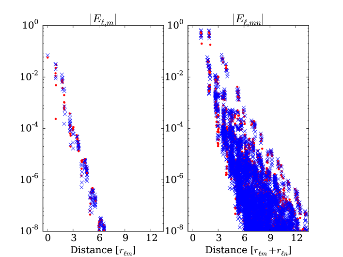
Figure 5.2: Locality of the site energy for the tight-binding toy model described in § 5.1. Red dots denote configuration (1), while blue crosses denote configuration (2).

5.3 Convergence rate

In our second numerical experiment we confirm the prediction of Theorem 4.3. We adopt again the model from § 5.1. As reference configuration we choose a di-vacancy configuration,

$$\Lambda=A_{\rm tri}\mathbb{Z}^{2}\setminus\big{\{}(0,0),(1,0)\big{\}}.$$

Then, for increasing radii $R$ with associated buffer radii $R^{\rm buf}$,

$$\begin{array}[]{r|c|lllll}&R&3&4&6&8&11\\ \hline\cr\text{Set 1}&R^{\rm buf}&2.1&2.4&2.8&3.0&3.4\\ \text{Set 2}&R^{\rm buf}&1.0&1.7&1.7&2.0&2.0\\ \text{Set 3}&R^{\rm buf}&1.0&1.0&1.7&1.7&2.0\end{array}$$ (5.15)

we solve the problem (4.4). In Set 1 we have chosen $R^{\rm buf}=1+\log(R)$, while in Sets 2, 3 we have chosen smaller buffer radii to investigate the effect of these choices on the error in the numerical solution.

The computed solutions $\bar{u}_{R}$ are compared against a high-accuracy solution with $R=20,R^{\rm buf}=11$, which yields the convergence graphs displayed in Figure 5.3, fully confirming the analytical prediction. To measure errors, instead of $\|D\cdot\|_{\ell^{2}_{\gamma}}$, we employ the equivalent norm $\|D^{\rm nn}\cdot\|_{\ell^{2}}$ with $D^{\rm nn}u=(D_{\rho}u)_{\rho\in\pm A_{\rm tri}e_{i},i=1,2}$.

We do not observe a pronounced buffer size effect. This could have a number of reasons, such as the fact that we are not far enough in the asymptotic regime or simply that the model we are employing is “too local” to observe this. We will present more extensive numerical results with a wider variety of TB models in [18, 19].

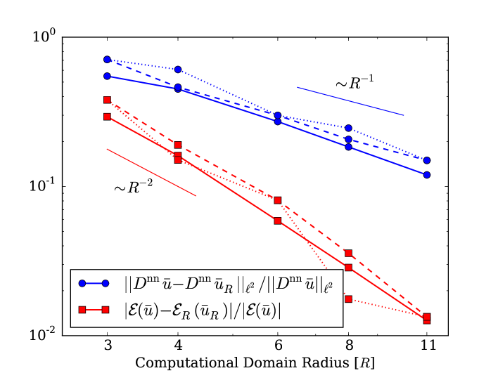
Figure 5.3: Convergence of (4.4) with increasing domain size $R$, as described in § 5.3. Set 1: full lines; Set 2: dashed lines; Set 3: dotted lines.

6 Concluding remarks

The main purpose of this paper was to set the scene for a rigorous numerical analysis approach to QM/MM coupling. We have achieved this by developing a new class of locality results for the tight binding model. Precisely, we have shown that the total band energy can be decomposed into contributions from individual sites in a meaningful, i.e. local, way.

This strong locality result is the basis for extending the theory of crystalline defects of [27], which we have hinted at in § 4.1, and carried out in detail in [17]. In further forthcoming articles [18, 19] we are employing it to develop new QM/MM coupling schemes for crystalline defects as well as their rigorous analysis.

A key question that remains to be investigated in the future, is whether our locality results extend to more accurate electronic structure models such as Kohn–Sham density functional theory. Understanding this extension is critical to take the theory we are developing in the present article and in [18, 19] towards materials science applications. However, there are many technical issues arising from the nonlinearity, the continuous nature, and in particular the long-range Coulomb interaction.

Appendix Appendix A Multiple orbitals per atom

We have assumed in § 2.1, and throughout this paper, that there is only one atomic orbital for each atom ($n_{\Xi}$=1). In this case, the symmetry assumption H.sym (i) is natural. However, in practical calculations, there are multiple atomic-like orbitals $\phi_{\ell\alpha}$ associated with each atomic site $\ell$. Here, $\alpha$ denotes both the orbital and angular quantum numbers of the atomic state. Many TB models employ one $s$-orbital $|s\rangle$, three $p$-orbitals $\{|x\rangle,~{}|y\rangle,~{}|z\rangle\}$ and five $d$-orbitals $\{|xy\rangle,~{}|yz\rangle,~{}|zx\rangle,~{}|x^{2}-y^{2}\rangle,~{}|3z^{2}-r^{2}\rangle\}$ per atom [29, 54]. Except for the $s$-orbital, all other orbitals have a spacial orientation, which means that the Hamiltonian matrix elements are not invariant under rotation/reflection. Therefore H.sym (i) is invalid and must be reformulated.

We assume in the following that $n_{\Xi}>1$ and $\{\phi_{\ell\alpha}\}_{1\leq\alpha\leq n_{\Xi}}$ is the set of atomic-like orbitals for the site $\ell$. The Hamiltonian can be expressed by (2.1),

$$\Big{(}\mathcal{H}(y)\Big{)}_{\ell k}^{\alpha\beta}=\int_{\mathbb{R}^{d}}\phi_{\ell\alpha}({\bf r}-y(\ell))\widehat{\mathcal{H}}(y)\phi_{k\beta}({\bf r}-y(k))~{}{\rm d}{\bf r}.$$ (A.1)

Applying an isometry $g$ to $y$, we obtain

$$\Big{(}\mathcal{H}\big{(}g(y)\big{)}\Big{)}_{\ell k}^{\alpha\beta}=\int_{\mathbb{R}^{d}}\phi_{\ell\alpha}\big{(}{\bf r}-g(y(\ell))\big{)}\widehat{\mathcal{H}}\big{(}g(y)\big{)}\phi_{k\beta}\big{(}{\bf r}-g(y(k))\big{)}~{}{\rm d}{\bf r}.$$ (A.2)

For simplicity of notation, we define

$$\psi_{\ell\alpha}({\bf r})=\phi_{\ell\alpha}\Big{(}g^{-1}({\bf r})-y(\ell)\Big{)}\quad{\rm and}\quad\varphi_{\ell\alpha}({\bf r})=\phi_{\ell\alpha}\Big{(}{\bf r}-g\big{(}y(\ell)\big{)}\Big{)}.$$

We assume that the two sets of atomic orbitals $\{\psi_{\ell\alpha}\}_{1\leq\alpha\leq n_{\Xi}}$ and $\{\varphi_{\ell\alpha}\}_{1\leq\alpha\leq n_{\Xi}}$ span the same subspace. This is true for almost all tight-binding models since the set of the atomic orbitals always include all three $p-$orbitals (if the $p-$orbital is involved) and all five $d-$orbitlas (if the $d-$orbital is involved). Then, there exists an orthogonal matrix $Q^{\ell}\in\mathbb{R}^{n_{\Xi}\times n_{\Xi}}$ such that $\varphi_{\ell\alpha}=\sum_{1\leq\beta\leq n_{\Xi}}Q^{\ell}_{\alpha\beta}\psi_{\ell\beta}$. We have from (A.2) that

$$\Big{(}\mathcal{H}\big{(}g(y)\big{)}\Big{)}_{\ell k}^{\alpha\beta} = \int_{\mathbb{R}^{d}}\varphi_{\ell\alpha}({\bf r})\widehat{\mathcal{H}}\big{(}g(y)\big{)}\varphi_{k\beta}({\bf r})~{}{\rm d}{\bf r}$$ (A.3)

$$= \sum_{1\leq\alpha^{\prime},\beta^{\prime}\leq n_{\Xi}}Q^{\ell}_{\alpha\alpha^{\prime}}Q^{k}_{\beta\beta^{\prime}}\int_{\mathbb{R}^{d}}\psi_{\ell\alpha^{\prime}}({\bf r})\widehat{\mathcal{H}}\big{(}g(y)\big{)}\psi_{k\beta^{\prime}}({\bf r})~{}{\rm d}{\bf r}.$$

Since $g$ is an isometry, it is natural to assume that

$$\Big{(}\mathcal{H}(y)\Big{)}_{\ell k}^{\alpha\beta}=\int_{\mathbb{R}^{d}}\psi_{\ell\alpha}({\bf r})\widehat{\mathcal{H}}\big{(}g(y)\big{)}\psi_{k\beta}({\bf r})~{}{\rm d}{\bf r}.$$ (A.4)

Let $\Big{(}\mathcal{H}(y)\Big{)}_{\ell k}:=\left[\Big{(}\mathcal{H}(y)\Big{)}_{\ell k}^{\alpha\beta}\right]_{1\leq\alpha,\beta\leq n_{\Xi}}\in\mathbb{R}^{n_{\Xi}\times n_{\Xi}}$ denote the local Hamiltonian, then we have from (A.3) and (A.4) that

$$\Big{(}\mathcal{H}\big{(}g(y)\big{)}\Big{)}_{\ell k}=Q^{\ell}\cdot\Big{(}\mathcal{H}(y)\Big{)}_{\ell k}\cdot\left(Q^{k}\right)^{\rm T},$$ (A.5)

which yields

$$\mathcal{H}\big{(}g(y)\big{)}=Q\cdot\mathcal{H}(y)\cdot Q^{\rm T}\quad{\rm with}\quad Q={\rm diag}\left\{Q^{1},\cdots,Q^{N}\right\}.$$ (A.6)

Note that $Q^{\ell}$ are orthogonal matrices, hence $Q$ is orthogonal as well. Therefore, the spectrum of $\mathcal{H}(y)$ and $\mathcal{H}\big{(}g(y)\big{)}$ are equivalent:

$$\epsilon_{s}=\epsilon_{s}^{g}\qquad{\rm for}~{}~{}1\leq s\leq N\cdot n_{\Xi}.$$ (A.7)

Let

$$\Psi_{s}=\left(\begin{array}[]{c}\Psi_{s}^{1}\\ \vdots\\ \Psi_{s}^{N}\end{array}\right)\quad{\rm with}\quad\Psi_{s}^{\ell}=\left(\begin{array}[]{c}\Psi_{s}^{\ell 1}\\ \vdots\\ \Psi_{s}^{\ell n_{\Xi}}\end{array}\right)\qquad{\rm for}~{}~{}1\leq s\leq N\cdot n_{\Xi}$$

be the eigenfunction of $\mathcal{H}(y)$ corresponding to the eigenvalue $\epsilon_{s}$. Then the corresponding eigenfunction of $\mathcal{H}\big{(}g(y)\big{)}$ is

$$\Psi_{s}^{g}=Q\Psi_{s}=\left(\begin{array}[]{c}Q^{1}\Psi_{s}^{1}\\ \vdots\\ Q^{N}\Psi_{s}^{N}\end{array}\right).$$ (A.12)

Next we note that, with multiple orbitals per atom, the expression (2.42) should be rewritten as

$$E_{\ell}(y)=\sum_{s}f(\varepsilon_{s})\varepsilon_{s}\sum_{\alpha}\left(\Psi_{s}^{\ell\alpha}\right)^{2}=\sum_{s}\mathfrak{f}(\varepsilon_{s})\sum_{\alpha}\left(\Psi_{s}^{\ell\alpha}\right)^{2}.$$ (A.13)

Taking into account (A.7), (A.12) and (A.13) we obtain invariance of the site energy under isometries,

$$E_{\ell}(y)=E_{\ell}(g(y)),$$ (A.14)

To summarize, in the case of multiple orbitals, the assumption H.sym (i) should become

H.sym’ (i). If $y\in\mathcal{V}_{\mathfrak{m}}^{N}$ and $g:\mathbb{R}^{d}\rightarrow\mathbb{R}^{d}$ is an isometry on $\mathbb{R}^{d}$, then there exist orthogonal matrices $Q^{\ell}\in\mathbb{R}^{n_{\Xi}\times n_{\Xi}}$ for $\ell=1,\cdots,N$ such that (A.6) is satisfied.

(This is equivalent to H.sym (i) when $n_{\Xi}=1$.)

Remark A.1.

Slater and Koster worked out expressions such as (A.5) and (A.6) for all integrals between $s$, $p$ and $d$ orbitals and presented them in Table 1 of their paper [54]. This has been invaluable for practical calculations, see, e.g. [29, 52].

Remark A.2.

We stress again that all our assumptions and analysis in the present paper can be extended to the multi-orbital case without any difficulty, by taking the Hamiltonian as a block matrix with

$$h_{\ell k}(y)=\Big{(}\mathcal{H}(y)\Big{)}_{\ell k}\in\mathbb{R}^{n_{\Xi}\times n_{\Xi}}$$ (A.15)

and $|h_{\ell k}(y)|$ the Frobenius norm of the submatrix.

Appendix Appendix B Site energy with non-orthogonal orbitals

We consider the tight binding model with non-orthogonal atomic orbitals in this appendix. It has been shown in Remark 2.1 (iv) that the transformed Hamiltonian is

$$\widetilde{\mathcal{H}}=\mathcal{M}^{-1/2}\mathcal{H}\mathcal{M}^{-1/2}$$

when the overlap matrix is not an identity matrix. Then the transformed eigenvectors of $\mathcal{H}\psi_{s}=\varepsilon_{s}\psi_{s}$ become $\tilde{\psi}_{s}=\mathcal{M}^{1/2}\psi_{s}$, and following (2.41), the site energy is given by

$$E_{\ell}(y)=\sum_{s}f(\varepsilon_{s})\varepsilon_{s}[\tilde{\psi}_{s}]_{\ell}^{2}=\sum_{s}\mathfrak{f}(\varepsilon_{s})[\mathcal{M}^{1/2}\psi_{s}]_{\ell}^{2}.$$ (B.1)

Since the square root of a matrix in (B.1) introduces additional computational cost for the site energy computations, we modify the definition of site energy in practice by

$$\widetilde{E}_{\ell}(y)=\sum_{s}\mathfrak{f}(\varepsilon_{s})[\mathcal{M}\psi_{s}]_{\ell}[\psi_{s}]_{\ell}.$$ (B.2)

The following result states that the modified site energy (B.2) preserves the locality property.

Lemma B.1.

Assume that L, H.tb, H.loc, F are satisfied, and moreover, the overlap matrix $\mathcal{M}$ satisfy the same conditions as those in H.tb, H.loc.

Then, for $1\leq j\leq\mathfrak{n}$, there exist positive constants $\tilde{C}_{j}$ and $\tilde{\eta}_{j}$ such that for any $\ell\in\Lambda_{N}$,

$$\left|\frac{\partial^{j}\widetilde{E}_{\ell}(y)}{\partial[y(m_{1})]_{i_{1}}\cdots\partial[y(m_{j})]_{i_{j}}}\right|\leq\tilde{C}_{j}e^{-\tilde{\eta}_{j}\sum_{l=1}^{j}|y(\ell)-y(m_{l})|}\qquad 1\leq i_{1},\cdots,i_{j}\leq d.$$ (B.3)

Proof.

Let $\varXi=\mathfrak{f}(\widetilde{\mathcal{H}})$ (with $\varXi_{jk}=\sum_{s}\mathfrak{f}(\varepsilon_{s})[\tilde{\psi}_{s}]_{j}[\tilde{\psi}_{s}]_{k}$). The assumptions on $\mathcal{H}$ and $\mathcal{M}$ imply that the transformed Hamiltonian $\widetilde{\mathcal{H}}$ also satisfies the conditions in H.tb and H.loc. Using Lemma 2.2 and similar arguments as those in the proof of Lemma 2.3, we have

$$|\varXi_{jk}|\leq Ce^{-\gamma|y(j)-y(k)|}\quad{\rm and}\quad\bigg{|}\frac{\partial\varXi_{jk}}{\partial[y(n)]_{i}}\bigg{|}\leq Ce^{-\gamma(|y(n)-y(j)|+|y(n)-y(k)|)}$$ (B.4)

with some constants $C$ and $\gamma$. Similarly, the assumptions on $\mathcal{M}$ also imply

$$\big{|}\mathcal{M}^{\pm 1/2}_{jk}\big{|}\leq Ce^{-\gamma|y(j)-y(k)|}\quad{\rm and}\quad\Bigg{|}\frac{\partial\mathcal{M}^{\pm 1/2}_{jk}}{\partial[y(n)]_{i}}\Bigg{|}\leq Ce^{-\gamma(|y(n)-y(j)|+|y(n)-y(k)|)}.$$ (B.5)

We have from (B.1) and (B.2) that

$$E_{\ell} =\sum_{s}\mathfrak{f}(\varepsilon_{s})\sum_{jk}\mathcal{M}^{1/2}_{\ell j}\mathcal{M}^{1/2}_{\ell k}[\psi_{s}]_{j}[\psi_{s}]_{k}=\varXi_{\ell\ell},$$

$$\widetilde{E}_{\ell} =\sum_{s}\mathfrak{f}(\varepsilon_{s})\sum_{j}\mathcal{M}_{\ell j}[\psi_{s}]_{j}[\psi_{s}]_{\ell}=[\mathcal{M}^{1/2}\varXi\mathcal{M}^{-1/2}]_{\ell\ell}.$$

Therefore,

$$\frac{\partial\widetilde{E}_{\ell}}{\partial[y(n)]_{i}}=\sum_{jk}\left(\frac{\partial\mathcal{M}^{1/2}_{\ell j}}{\partial[y(n)]_{i}}\varXi_{jk}\mathcal{M}^{-1/2}_{k\ell}+\mathcal{M}^{1/2}_{\ell j}\frac{\partial\varXi_{jk}}{\partial[y(n)]_{i}}\mathcal{M}^{-1/2}_{k\ell}+\mathcal{M}^{1/2}_{\ell j}\varXi_{jk}\frac{\partial\mathcal{M}^{-1/2}_{k\ell}}{\partial[y(n)]_{i}}\right),$$

which together with (B.4), (B.5), and a similar argument as that in (2.49) completes the proof of (B.3) for $j=1$.

The proofs for $2\leq j\leq\mathfrak{n}$ are similar. ∎

References

- [1] R. Baer and M. Head-Gordon, Sparsity of the density mtrix in kohn-sham density functional theory and an assessment of linear system-size scaling methods, Phys. Rev. Lett., 79 (1997), pp. 3962–3965.
- [2] M. Benzi, P. Boito, and N. Razouk, Decay properties of spectral projectors with applications to electronic structure, SIAM Review, 55 (2013), pp. 3–64.
- [3] N. Bernstein, J. Kermode, and G. Csányi, Hybrid atomistic simulation methods for materials systems, Rep. Prog. Phys., 72 (2009), pp. 26051 1–25.
- [4] J. Bezanson, A. Edelman, S. Karpinski, and V. B. Shah, Julia: A fresh approach to numerical computing, arXiv e-Prints, 1411.1607 (2014).
- [5] X. Blanc, C. L. Bris, and P.-L. Lions, From molecular models to continuum mechanics, Arch. Rat. Mech. Anal., 164 (2002), pp. 341–381.
- [6] , On the energy of some microscopic stochastic lattices, Part I, Arch. Rat. Mech. Anal., 184 (2007), pp. 303–340.
- [7] D. Bowler and T. Miyazaki, O(N) methods in electronic structure calculations, Rep. Progr. Phys., 75 (2012), pp. 036503–036546.
- [8] E. Cancès and C. L. Bris, Mathematical modeling of point defects in materials science, Math. Models Methods Appl. Sci., 23 (2013), pp. 1795–1859.
- [9] E. Cancès, A. Deleurence, and M. Lewin, A new approach to the modelling of local defects in crystals: The reduced Hartree-Fock case, Commun. Math. Phys., 281 (2008), pp. 129–177.
- [10] , Non-perturbative embedding of local defects in crystalline materials, J. Phys.: Condens. Mat., 20 (2008), pp. 294213 1–6.
- [11] E. Cancès and V. Ehrlacher, Local defects are always neutral in the Thomas-Fermi-von Weiszäcker theory of crystals, Arch. Ration. Mech. Anal., 202 (2011), pp. 933–973.
- [12] E. Cancès, S. Lahbabi, and M. Lewin, Mean-field models for disordered crystals, J. Math. Pures Appl., 100 (2013), pp. 241–274.
- [13] E. Cancès and M. Lewin, The dielectric permittivity of crystals in the reduced Hartree-Fock approximation, Arch. Ration. Mech. Anal., 197 (2010), pp. 139–177.
- [14] E. Cancès and N. Mourad, A mathematical perspective on density functional perturbation theory. arXiv:1405.1348.
- [15] I. Catto, C. L. Bris, and P.-L. Lions, The Mathematical Theory of Thermodynamic Limits: Thomas-Fermi Type Models, Oxford Mathematical Monographs, Hardcover, 1998.
- [16] , On the thermodynamic limit for Hartree-Fock type models, Ann. I. H. Poincaré, An., 18 (2001), pp. 687–760.
- [17] H. Chen, Q. Nazar, and C. Ortner, Variational problems for crystalline defects. in preparation.
- [18] H. Chen and C. Ortner, Construction and analysis of energy-based QM/MM hybrid methods. in preparation.
- [19] , Construction and analysis of force-based QM/MM hybrid methods. in preparation.
- [20] J. Combes and L. Thomas, Asymptotic behaviour of eigenfunctions for multiparticle schrödinger operators, Commun. Math. Phys., 34 (1973), pp. 251–270.
- [21] G. Csányi, T. Albaret, G. Moras, M. Payne, and A. D. Vita, Multiscale hybrid simulation methods for material systems, J. Phys,: Condens. Matter, 17 (2005), pp. 691–703.
- [22] G. Csányi, T. Albaret, M. Payne, and A. D. Vita, “Learn on the fly”: a hybrid classical and quantum-mechanical molecular dynamics simulation, Phys. Rev. Lett., 93 (2004), pp. 175503 1–4.
- [23] W. E and J. Lu, The elastic continuum limit of the tight binding model, Chin. Ann. Math. Ser. B, 28 (2007), pp. 665–675.
- [24] , The electronic structure of smoothly deformed crystals: Cauchy-born rule for the nonlinear tight-binding model, Comm. Pure Appl. Math., 63 (2010), pp. 1432–1468.
- [25] , The electronic structure of smoothly deformed crystals: Wannier functions and the cauchy-born rule, Arch. Ration. Mech. Anal., 199 (2011), pp. 407–433.
- [26] , The Kohn-Sham equation for deformed crystals, Mem. Amer. Math. Soc., vol. 221, no. 1040, 2013.
- [27] V. Ehrlacher, C. Ortner, and A. Shapeev, Analysis of boundary conditions for crystal defect atomistic simulations. arXiv:1306.5334.
- [28] F. Ercolessi, Lecture notes on tight-binding molecular dynamics and tight-binding justification of classical potentials. Lecture notes 2005.
- [29] M. Finnis, Interatomic Forces in Condensed Matter, Oxford University Press, Oxford, 2003.
- [30] C. Fu and K. Ho, First-principles calculation of the equilibrium ground-state properties of transition metals: Applications to nb and mo, Phys. Rev. B, 28 (1983), pp. 5480–5486.
- [31] J. Gao and D. Truhlar, Quantum mechanical methods for enzyme kinetics, Annu. Rev. Phys. Chem., 53 (2002), pp. 467–505.
- [32] S. Goedecker, Integral representation of the fermi distribution and its applications in electronic-structure calculations, Phys. Rev. B, 48 (1993), pp. 17573–17575.
- [33] , Linear scaling electronic structure methods, Rev. Mod. Phys., 71 (1999), pp. 1085–1123.
- [34] S. Goedecker and M. Teter, Tight-binding electronic-structure calculations and tight-binding molecular dynamics with localized orbitals, Phys. Rev. B, 51 (1995), pp. 9455–9464.
- [35] C. Goringe, D. Bowler, and E. Hernández, Tight-binding modelling of materials, Rep. Prog. Phys., 60 (1997), pp. 1447–1512.
- [36] R. Horn and C. Johnson, Matrix Analysis, Cambridge University Press, Cambridge, 1991.
- [37] S. Ismail-Beigi and T. Arias, Locality of the density matrix in metals, semiconductors, and insulators, Phys. Rev. Lett., 82 (1999), pp. 2127–2130.
- [38] J. Kermode, T. Albaret, D. Sherman, N. Bernstein, P. Gumbsch, M. Payne, G. Csányi, and A. D. Vita, Low-speed fracture instabilities in a brittle crystal, Nature, 455 (2008), pp. 1224–1227.
- [39] W. Kohn, Analytic properties of bloch waves and wannier functions, Phys. Rev., 115 (1959), pp. 809–821.
- [40] M. Kohyama and R. Yamamoto, Tight-binding study of grain boundaries in si: Energies and atomic structures of twist grain boundaries, Phys. Rev. B, 49 (1994), pp. 17102–17117.
- [41] G. Kresse and J. Furthmüller, Efficient iterative schemes for ab initio total-energy calculations using a plane-wave basis set, Phys. Rev. B, 54 (1996), pp. 11169–11186.
- [42] S. Lahbabi, The reduced Hartree-Fock model for short-range quantum crystals with nonlocal defects, Ann. Henri Poincaré, 15 (2014), pp. 1403–1452.
- [43] S. Lee, J. Dow, and O. Sankey, Theory of charge-state splittings of deep levels, Phys. Rev. B, 31 (1985), pp. 3910–3914.
- [44] E. Lieb and B. Simon, The Thomas-Fermi theory of atoms, molecules and solids, Advances in Math., 23 (1977), pp. 22–116.
- [45] L. Lin, J. Lu, L. Ying, and W. E, Pole-based approximation of the fermi-dirac function, Chin. Ann. Math. B, 30 (2009), pp. 729–742.
- [46] M. Luskin and C. Ortner, Atomistic-to-continuum coupling, Acta Numerica, (2013).
- [47] P. Motamarria, M. Nowakb, K. Leiterc, J. Knapc, and V. Gavini, Higher-order adaptive finite-element methods for Kohn-Sham density functional theory, J. Comp. Phys., 253 (2013), pp. 308–343.
- [48] F. Nazar and C. Ortner. manuscript.
- [49] R. Nunes, J. Bennetto, and D. Vanderbilt, Structure, barriers, and relaxation mechanisms of kinks in the 90° partial dislocation in silicon, Phys. Rev. Lett., 77 (1996), pp. 1516–1519.
- [50] S. Ogata, E. Lidorikis, F. Shimojo, A. Nakano, P. Vashishta, and R. Kalia, Hybrid finite-element/molecular-dynamic/electronic-density-functional approach to materials simulations on parallel computers, Comput. Phys. Commun., 138 (2001), pp. 143–154.
- [51] C. Ortner and F. Theil, Justification of the cauchy-born approximation of elastodynamics, Arch. Ration. Mech. Anal., 207 (2013), pp. 1025–1073.
- [52] D. Papaconstantopoulos, Handbook of the Band Structure of Elemental Solids, From Z = 1 To Z = 112, Springer New York, 2015.
- [53] E. Prodan and W. Kohn, Nearsightedness of electronic matter, Proc. Natl. Acad. Sci. USA, 102 (2005), pp. 11635–11638.
- [54] J. Slater and G. Koster, Simplified lcao method for the periodic potential problem, Phys. Rev., 94 (1954), pp. 1498–1524.
- [55] J. Tersoff, New empirical approach for the structure and energy of covalent systems, Phys. Rev. B, 37 (1988), pp. 6991–7000.
- [56] C. Wang, C. Chan, and K. Ho, Tight-binding molecular-dynamics study of defects in silicon, Phys. Rev. Lett., 66 (1991), pp. 189–192.
- [57] Y. Wang, G. Stocks, W. Shelton, D. Nicholson, Z. Szotek, and W. Temmerman, Order-N multiple scattering approach to electronic structure calculations, Phys. Rev. Lett., 75 (1995), pp. 2867–2870.
- [58] A. Warshela and M. Levitta, Theoretical studies of enzymic reactions: Dielectric, electrostatic and steric stabilization of the carbonium ion in the reaction of lysozyme, Journal of Molecular Biology, 103 (1976), pp. 227–249.
- [59] H. Yukawa, On the interaction of elementary particles, Proc. Phys. Math. Soc. Japan., 17 (1935), pp. 48–57.