Josephson Currents and Spin Transfer Torques in Ballistic SFSFS Nanojunctions

Abstract

Utilizing a full microscopic Bogoliubov-de Gennes (BdG) approach, we study the equilibrium charge and spin currents in ballistic $SFSFS$ Josephson systems, where $F$ is a uniformly magnetized ferromagnet and $S$ is a conventional $s$-wave superconductor. From the spatially varying spin currents, we also calculate the associated equilibrium spin transfer torques. Through variations in the relative phase differences between the three $S$ regions, and magnetization orientations of the ferromagnets, our study demonstrates tunability and controllability of the spin and charge supercurrents. The spin transfer torques are shown to reveal details of the proximity effects that play a crucial role in these types of hybrid systems. The proposed $S$$F$$S$$F$$S$ nanostructure is discussed within the context of a superconducting magnetic torque transistor.

I Introduction

Proximity effects inherent to superconducting systems with inhomogeneous magnetic order presents a mechanism by which dissipationless current flow and the spin degree-of-freedom can both be effectively coupled and controlled.bergeret1 ; eschrigh1 ; efetov1 ; golubov1 ; buzdin1 ; shay The important role that proximity effects play in the static and transport properties of ferromagnetic Josephson junctions with $s$-wave superconductors is now well established. Indeed, the proximity induced damped oscillatory superconducting correlations within the ferromagnet region serves as a channel for interlayer coupling and spin switching bergeret1 ; eschrigh1 ; buzdin1 ; alidoust_sfsfs ; waintal_1 ; halter_tc ; halter_gr_tc . Proximity induced triplet pairing correlations within the ferromagnetic junction also provides another avenue for spin transport.Eschrig_1 ; Eschrig_2 ; halter_trplt ; halter_trplt2 Interest in Josephson junctions with ferromagnetic layers has grown due to their possibility as serving as elements in next generation superconducting computing and nonvolatile memories,eschrigh1 ; efetov1 ; golubov1 ; buzdin1 where single flux quantum circuits containing multiple Josephson junction arrangements can improve switching speeds.giaz1 ; giaz3 ; alidoust_mgmtr To determine whether Josephson structures can serve as viable cryogenic spintronic devices, it is crucial to understand the behavior of the spin currents that can flow in such systems. The spin current flowing into the ferromagnetic regions exerts a torque on the magnetization if the current polarization direction is noncollinear to the local magnetization in the ferromagnet. In other words, the spin angular momentum of the polarized current will be partially transferred to the magnetization in the $F$ region.STT_1 ; STT_2 This spin transfer torque (STT) serves as an important mechanism in spintronics devices.STT_1 ; STT_2 ; linder1 The STT effect can cause magnetization switching for sufficiently large currents without the need for an external field. This switching aspect provides a unique opportunity to create and improve fast-switching magnetic random access memories. zutic_rmp ; fert_rmp ; brataas_nat ; Bauer_nat

The recent experimental pursuits of spin-based memory technologies involving various arrangements of $S$$F$$S$ Josephson junctions has rekindled interest in the realm of ferromagnetic Josephson arrays.alidoust_sfsfs ; buzdin_sfsfs ; ryaz1 ; ryaz2 ; ryaz3 ; ryaz4 ; Kupriyanov1 When a sequence of $S$$F$$S$ junctions are placed in a series configuration, creating a $S$$F$$S$$F$$S$ type junction shown in Fig. 1, additional possibilities emerge for the control of the associated spin and charge supercurrents.alidoust_sfsfs ; buzdin_sfsfs For example, the triplet components of the supercurrent and total charge transport in diffusive $S$$F$$S$$F$$S$ structures is closely linked to the relative magnetization orientations, which can directly alter the total charge current flow, causing it to reverse direction in the ferromagnetic layers.alidoust_sfsfs The transport of triplet supercurrents through the middle $S$ electrode can be utilized to manipulate the magnetic moment of the $F$ layers in $S$$F$$S$$F$$S$ hybrids.buzdin_sfsfs The spin-polarized supercurrents in these types of systems may also be used to induce a STT acting on the magnetization of a ferromagnet.waintal_1 ; waintal_2 ; Zhao ; alidoust_spn

At the interfaces between the $F$ and $S$ regions in a ballistic $S$$F$$S$$F$$S$ Josephson junction, quasiparticles undergo Andreev and conventional reflections.radovic2 ; radovic1 ; beenaker2 ; beenaker1 Besides the contribution from the continuum states, the superposition and interference of the corresponding quasiparticle wavefunctions in the $F$ regions result in subgap bound states that contribute to the total current flow between the $S$ banks. By varying the width of the central $S$ layer, $d_{S}$, modifications to the Andreev bound state spectra can ensue, i.e., by simply decreasing $d_{S}$, additional overlap can occur between the subgap bound states in the adjacent $F$ regions.Freyn1 ; Chang1 ; Averin For $S$$F$$S$$F$$S$ type structures, if the central $S$ layer is sufficiently thin, i.e., $d_{S}\lesssim\xi$, the proximity effects within the interacting $F$ regions result in the Cooper pair amplitude and local density of states in each $F$ region being mutually altered. Therefore, magnetization rotation in a single $F$ layer can strongly influence the thermodynamic and quantum transport properties throughout the rest of the system. The coupling between the different regions can then result in the system residing in a ground state corresponding to a phase difference of $\Delta\varphi=\pi$.alidoust_sfsfs ; trifunovic The appearance of superharmonic Josephson currents (with second and higher harmonics: $\sin 2\varphi$, $\sin 3\varphi$, …) were theoretically predicted to appear in nonequilibrium and point contact Josephson junctions2th_hrmnc_1 . Shortly thereafter, the higher harmonic supercurrents were experimentally observed in nonequilibrium situations2th_hrmnc_2 . Also, it was shown theoretically for a uniform $S$$F$$S$ junction, that the higher harmonics can be revealed at the $0$-$\pi$ transition point, where the first harmonic is highly suppressed due to the supercurrent flow reversing direction at that point.buzdin1 ; golubov1 Therefore, the nonvanishing supercurrent at the $0$-$\pi$ transition point observed experimentally in Ref. ryaz0, was soon attributed to the presence of higher harmonics2th_hrmnc_3 ; buzdin1 ; zareyan ; alidoust_spn . Subsequent works with ferromagnetic Josephson junctions demonstrated that the higher harmonics can naturally arise when varying the location of domain wallsklaus_domain , and in ballistic double magnetic $S$$F$$F$$S$ junctions, provided that the thickness of the magnetic layers are unequaltrifunovic . Recently, evidence of higher harmonics has been experimentally observed in Josephson junctions with spin dependent tunneling barriers.pure_2th_hrmnc

The focus of this paper is to theoretically investigate proximity effects leading to modified superconducting correlations and controlled charge and spin transport in $S$$F$$S$$F$$S$ ballistic junctions. We will address a variety of relative magnetization orientations, and prescribed superconducting macroscopic phase differences between the $S$ terminals. Utilizing a microscopic Bogoliubov-de Gennes (BdG) approach, we derive the appropriate expressions for the charge and spin currents and the corresponding equilibrium spin transfer torques. The numerical solutions to the BdG equations are employed to study the current phase relations, revealing the emergence of additional harmonics that depend on the tunable magnetization profile and other system parameters. We demonstrate that our proposed $S$$F$$S$$F$$S$ systems can be considered as a superconducting magnetic torque transistor, where the flow of spin and charge currents can be tuned by the macroscopic phases of the superconducting leads. This, in turn, dictates the torques acting on the exchange fields of the $F$ layers. Remarkably, the superconducting phases (in addition to other system parameters) can effectively switch the torques acting on the magnetizations of the $F$ layers ‘on’ or ‘off’. The directions of the torques and charge currents are shown to not be related by simple functions of the phase differences or exchange fields, similar to what was observed in simpler ferromagnetic Josephson junctions involving equilibrium torques. waintal_1 We also find that when the angle describing the relative in-plane magnetic exchange field orientations is varied, the torque tending to align the two $F$ magnetizations is usually largest for relative magnetization angles other than the expected orthogonal configurations. Moreover, we have found that these sequential nanodevices allow for detecting pure second harmonics in the current phase relations, depending on the system parameters, including the relative magnetization orientations. We present a study of the crossover between the first and second harmonic in the current phase relations and consider experimentally feasible situations to observe them. This crossover is discussed in the context of the appearance of equal spin triplet correlations with $m=\pm 1$ spin projections along the spin quantization axis.

The paper is organized as follows. In Sec. II, we outline the theoretical approach used and derivation of various physical quantities investigated, including the supercurrent, magnetization, spin current, and associated torques. We present our results in Sec. III. This section is divided into two-subsections: Subsect. III.1 presents the current phase relations and the second harmonic supercurrents that can be generated by calibrating the system parameters. Subsect. III.2, discusses the associated spin currents and equilibrium spin transfer torques. Finally, we give concluding remarks in Sec. IV.

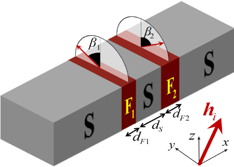
Figure 1: (Color online) Schematic of the $S$$F$$S$$F$$S$ ballistic heterojunction considered in this paper. The system is infinite in the $yz$ plane, and thus the $x$ axis is normal to the plane of the interfaces. The middle $S$ electrode has a thickness $d_{S}$ in the $x$ direction, and is sandwiched between two $F$ layers with unequal thicknesses $d_{F1}$ and $d_{F2}$. The $F$ layers are uniformly magnetized and their exchange fields are denoted by ${\bm{h}}_{i}$ (for $i=1,2$). To simplify notation, we have defined the magnetization directions via: ${\bm{h}}_{i}=|{\bm{h}}_{i}|(\cos\alpha_{i},\sin\alpha_{i}\sin\beta_{i},\sin\alpha_{i}\cos\beta_{i})$. The $S$ electrodes can take arbitrary phases, described by $\varphi_{L}$, $\varphi_{M}$, and $\varphi_{R}$ for the left, middle and right $S$ electrodes, respectively.

II Theoretical Method

We begin our methodology by introducing the Bogoliubov-de Gennes (BdG) formalism.Gennes The BdG approach is a convenient microscopic quantum mechanical technique that allows a complete investigation into the fundamental characteristics of the superconductivity of ballistic superconducting heterojunctions. The microscopic BdG formalism can easily accommodate a broad range of magnetic exchange field strengths and profiles, including the half-metallic limit where the magnitude of the exchange field and the Fermi energy, $\varepsilon_{F}$, are the sameklaus . A schematic of the multilayer configuration that we study is depicted in Fig. 1. For this quasi one-dimensional system, physical quantities are invariant with respect to the $yz$ plane, while the $x$-direction captures the essential physical characteristics of the system. The corresponding spin-dependent BdG equations are thus expressed as,

$$\begin{bmatrix}{\cal H}_{0}-h_{z}&-h_{x}+ih_{y}&0&\Delta(x)\\ -h_{x}-ih_{y}&{\cal H}_{0}+h_{z}&\Delta(x)&0\\ 0&\Delta^{*}(x)&-({\cal H}_{0}-h_{z})&-h_{x}-ih_{y}\\ \Delta^{*}(x)&0&-h_{x}+ih_{y}&-({\cal H}_{0}+h_{z})\end{bmatrix}\Psi_{n}(x)$$

$$\hskip 36.135pt=\epsilon_{n}\Psi_{n}(x),$$ (1)

where $\Psi_{n}(x)\equiv(u_{n\uparrow}(x),u_{n\downarrow}(x),v_{n\uparrow}(x),v_{n\downarrow}(x))^{\mathbb{T}}$, and $u_{n\sigma}$ and $v_{n\sigma}$ are the quasiparticle and quasihole amplitudes. The pair potential $\Delta(x)$, which effectively scatters electrons into holes (and vice versa) is nonzero only in the superconducting electrode regions. We furthermore assume that $\Delta(x)$ is piecewise constant in the $S$ regions, with each $S$ region possessing the same magnitude but possibly different phase. Thus, within the external $S$ electrodes, $\Delta(x)$ takes the form $\Delta_{0}e^{i\varphi_{L}}$ in the left, $\Delta_{0}e^{i\varphi_{M}}$ in the middle, and $\Delta_{0}e^{i\varphi_{R}}$ in the right $S$ electrode. The combinations of phase differences involving $\varphi_{L}$, $\varphi_{M}$, and $\varphi_{R}$ results in additional possibilities for supercurrent flow compared to conventional Josephson junctions comprised of two superconducting banks. The single particle Hamiltonian ${\cal H}_{0}(x)$ is defined as,

$${\cal H}_{0}(x)=-\frac{1}{2m}\frac{\partial^{2}}{\partial x^{2}}+\varepsilon_{\perp}-\varepsilon_{F}+U(x),$$ (2)

where $\varepsilon_{\perp}=\frac{1}{2m}(k_{y}^{2}+k_{z}^{2})$ is the quasiparticle energy for motion in the invariant $yz$ plane (see Fig. 1), and the spin-independent scattering potential is denoted by $U({x})$. We represent the magnetism of the $F$ layers by a Stoner effective exchange energy ${\bm{h}}({x})$ which will in general have components in all $(x,y,z)$ directions. Additional technical details on solving the BdG equations for this type of quasi one-dimensional setup is given in the Appendix.

Various other types of “inverse” proximity effects sillanpaa ; halty ; berger can also occur in the vicinity of the $F/S$ contacts, whereby ferromagnetic order propagates from one $F$ layer to the other (creating a mutual torque) via the central $S$ layer. Therefore it is of interest to determine not only the spatial profile of the magnetization ${\bm{m}}({x})$ within the $F$ regions, but also within the central $S$ layer, where the induced magnetization can also screenklaus_emerge the magnetization of the adjacent ferromagnet. The complete spatial profiles of the magnetization are determined using the expressions: wu

$$m_{x}(x) =-\mu_{B}\sum_{n}\Bigl{\{}\Bigl{(}u^{*}_{n\uparrow}(x)u_{n\downarrow}(x)+u^{*}_{n\downarrow}(x)u_{n\uparrow}(x)\Bigr{)}f_{n}$$

$$-\Bigl{[}v_{n\uparrow}(x)v^{*}_{n\downarrow}(x)+v_{n\downarrow}(x)v^{*}_{n\uparrow}(x)\Bigr{]}(1-f_{n})\Bigr{\}}.$$ (3)

$$m_{y}(x) =-i\mu_{B}\sum_{n}\Bigl{\{}\Bigl{(}u_{n\uparrow}(x)u^{*}_{n\downarrow}(x)-u_{n\downarrow}(x)u^{*}_{n\uparrow}(x)\Bigr{)}f_{n}$$

$$+\Bigl{[}v_{n\uparrow}(x)v^{*}_{n\downarrow}(x)-v_{n\downarrow}(x)v^{*}_{n\uparrow}(x)\Bigr{]}(1-f_{n})\Bigr{\}}.$$ (4)

$$m_{z}(x) =-\mu_{B}\sum_{n}\Bigl{\{}\Bigl{[}|u_{n\uparrow}(x)|^{2}-|u_{n\downarrow}(x)|^{2}\Bigr{]}f_{n}$$

$$+\Bigl{[}|v_{n\uparrow}(x)|^{2}-|v_{n\downarrow}(x)|^{2}\Bigr{]}(1-f_{n})\Bigr{\}},$$ (5)

where $\mu_{B}$ is the Bohr magneton, and $f_{n}$ the Fermi function.

The Josephson effect leads to many possibilities for charge supercurrent transport in $SFSFS$ junctions. This experimentally accessible phenomenon is now well understood, with the primary driving mechanism being the difference between the macroscopic phases of two $S$ banks, separated by a weak link.Likharev ; Gennes ; josephson When there are three coupled $S$ banks, the situation becomes more complicated, and the dissipationless charge current depends on various combinations of the phase differences in addition to the other geometric and material properties of the system. When computing the supercurrent flowing in the $x$ direction, we express the Josephson current in terms of the quasiparticle amplitudes: Gennes ; klaus_domain

$${J_{x}}({x}) =\frac{2e}{m}\sum_{n}{\rm Im}\Biggl{\{}f_{n}\Bigl{[}u_{n\uparrow}{\frac{\partial u^{*}_{n\uparrow}}{\partial x}}+u_{n\downarrow}{\frac{\partial u^{*}_{n\downarrow}}{\partial x}}\Bigr{]}$$ (6)

$$+\left(1-f_{n}\right)\Bigl{[}v_{n\uparrow}{\frac{\partial v^{*}_{n\uparrow}}{\partial x}}+v_{n\downarrow}{\frac{\partial v^{*}_{n\downarrow}}{\partial x}}\Bigr{]}\Biggr{\}}.$$

Similarly, following the approach outlined in the Appendix, we can also write the spin current $S_{\sigma}$ with spin $\sigma$ flowing along the $x$ direction in terms of the quasiparticle amplitudes:

$${S}_{x}(x)=-\frac{i}{2m}\sum_{n}\Biggl{\{}f_{n}\Bigl{[}u_{n\uparrow}^{*}\frac{\partial u_{n\downarrow}}{\partial x}+u_{n\downarrow}^{*}\frac{\partial u_{n\uparrow}}{\partial x}-u_{n\downarrow}\frac{\partial u^{*}_{n\uparrow}}{\partial x}-u_{n\uparrow}\frac{\partial u^{*}_{n\downarrow}}{\partial x}\Bigr{]}$$

$$-(1-f_{n})\Bigl{[}v_{n\uparrow}\frac{\partial v^{*}_{n\downarrow}}{\partial x}+v_{n\downarrow}\frac{\partial v^{*}_{n\uparrow}}{\partial x}-v^{*}_{n\uparrow}\frac{\partial v_{n\downarrow}}{\partial x}-v^{*}_{n\downarrow}\frac{\partial v_{n\uparrow}}{\partial x}\Bigr{]}\Biggr{\}},$$ (7)

$${S}_{y}(x)=-\frac{1}{2m}\sum_{n}\Biggl{\{}f_{n}\Bigl{[}u_{n\uparrow}^{*}\frac{\partial u_{n\downarrow}}{\partial x}-u_{n\downarrow}^{*}\frac{\partial u_{n\uparrow}}{\partial x}-u_{n\downarrow}\frac{\partial u^{*}_{n\uparrow}}{\partial x}+u_{n\uparrow}\frac{\partial u^{*}_{n\downarrow}}{\partial x}\Bigr{]}$$

$$-(1-f_{n})\Bigl{[}v_{n\uparrow}\frac{\partial v^{*}_{n\downarrow}}{\partial x}-v_{n\downarrow}\frac{\partial v^{*}_{n\uparrow}}{\partial x}+v^{*}_{n\uparrow}\frac{\partial v_{n\downarrow}}{\partial x}-v^{*}_{n\downarrow}\frac{\partial v_{n\uparrow}}{\partial x}\Bigr{]}\Biggr{\}},$$ (8)

$${S}_{z}(x)=-\frac{i}{2m}\sum_{n}\Biggl{\{}f_{n}\Bigl{[}u_{n\uparrow}^{*}\frac{\partial u_{n\uparrow}}{\partial x}-u_{n\uparrow}\frac{\partial u^{*}_{n\uparrow}}{\partial x}-u^{*}_{n\downarrow}\frac{\partial u_{n\downarrow}}{\partial x}+u_{n\downarrow}\frac{\partial u^{*}_{n\downarrow}}{\partial x}\Bigr{]}$$

$$-(1-f_{n})\Bigl{[}-v_{n\uparrow}\frac{\partial v^{*}_{n\uparrow}}{\partial x}+v^{*}_{n\uparrow}\frac{\partial v_{n\uparrow}}{\partial x}+v_{n\downarrow}\frac{\partial v^{*}_{n\downarrow}}{\partial x}-v^{*}_{n\downarrow}\frac{\partial v_{n\downarrow}}{\partial x}\Bigr{]}\Biggr{\}},$$ (9)

where the sums for the currents above are in principle taken over all quasiparticle states.

III Results and discussions

We focus here on the low temperature regime, with $T/T_{c}=0.001$, where $T_{c}$ is the critical temperature of the corresponding bulk $S$ material. For simplicity we set $\varphi_{L}=0$, $\varphi_{M}=\varphi/2$, and $\varphi_{R}=\varphi$, for the phases of the left, middle, and right $S$ terminals, respectively. Thus, a phase difference of $\varphi/2$ is maintained across each $S$ electrode. The spatial variables are normalized in terms of the Fermi wavevector, including the BCS zero-temperature coherence length, $\xi_{0}$, set to $k_{F}\xi_{0}=100$, and the dimensionless position $X$, written as $X=k_{F}x$. For each physical quantity studied, a broad range of central $S$ widths will be considered. We assume that the ferromagnets are similar materials with identical exchange field strengths, i.e., $|{\bm{h}}_{1}|=|{\bm{h}}_{2}|=h$, set to the representative value of $h/\varepsilon_{F}=0.1$. To create favorable conditions for equal-spin triplet generation, trifunovic the ${F_{1}}$ and ${F_{2}}$ regions have highly asymmetric widths, with $d_{F1}=0.1\xi_{0}$, and $d_{F2}=3.8\xi_{0}$, so that $d_{F1}\ll d_{F2}$.

III.1 Josephson Charge Supercurrent

We begin with a discussion of the supercurrent charge transport by solving the microscopic BdG equations (Eq. (1)) over a broad range of energies and then summing the corresponding quasiparticle amplitudes and energies according to the expression given by Eq. (6). The charge current also can be obtained by minimizing the free energy with respect to the appropriate superconducting phase differences.Gennes Our microscopic method fully accounts for bound states that may be generated from quasiparticle trajectories with large momenta corresponding to in-plane energies comparable to $\varepsilon_{F}$ (shown to be important for $SNS$ junctionssagi ). The charge supercurrent is normalized by $J_{0}=nev_{F}$, where $v_{F}$ is the Fermi velocity, $e$ the electron charge, and $n$ is the number density. We focus our attention on supercurrents flowing through the ferromagnets, recalling that each of the three $S$ regions act as effective sources or sinks in the current. The pair potential $\Delta(x)$ of course vanishes in the intrinsically nonsuperconducting $F$ regions.

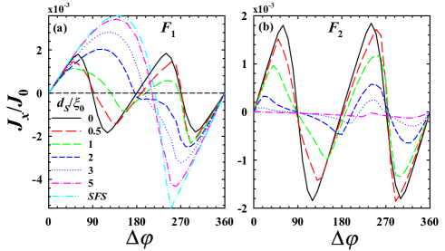
Figure 2: Normalized Josephson current versus the macroscopic phase difference of the two outermost electrodes, $\Delta\varphi$, in a $S$$F$$S$$F$$S$ structure with asymmetric ferromagnet widths of $d_{F1}/\xi_{0}=0.1$ and $d_{F2}/\xi_{0}=3.8$ (see Fig. 1). The width of the central $S$ electrode, $d_{S}$, varies as shown in the legend. The relative exchange fields between the two magnets is orthogonal with $\alpha_{1}=\alpha_{2}=90^{\rm o}$, $\beta_{1}=90^{\rm o}$ (along $y$), and $\beta_{2}=0^{\rm o}$ (along $z$). The phase of the middle $S$ electrode takes the value, $\varphi_{M}=\varphi/2$. For comparison, in (a) we show the results for a simpler $SFS$ junction having a phase difference $\Delta\varphi/2$ and $F$ width $d_{F1}=0.1\xi_{0}$.

To begin, in Fig. 2 the supercurrent is shown as a function of the phase difference, $\Delta\varphi$, for a wide range of central $S$ electrode widths, $d_{S}$. The central $S$ electrode acts as an external current source, and hence the spatial behavior of the current is piecewise constant in each $F$ region. Thus, each panel corresponds to the current in a particular ferromagnet (as labeled). The relative magnetic exchange fields are orthogonal, with ${\bm{h}}_{1}$ directed along $y$ and ${\bm{h}}_{2}$ along $z$ (see Fig. 1). Two limiting cases are shown: In the first case, the width of the central $S$ layer is zero ($d_{S}=0$), and in the second case, a large central layer ($d_{S}=5\xi_{0}$) is considered. When there is no middle $S$ layer, the current phase relation (CPR) is $\pi$-periodic, with behavior consistent with a ballistic $SFFS$ asymmetric double magnetic structuretrifunovic . For $d_{S}=5\xi_{0}$, the large $S$ width effectively decouples the two ferromagnets, creating two isolated $SFS$ junctions with phase differences $\varphi/2$. Thus, in this case one junction consists of a thin uniform $F_{1}$ region sandwiched by two superconductors, and its CPR reflects the overall behavior and direction reversal that is expected in narrow ferromagnetic $SFS$ Josephson junctions.golubov1 The other decoupled $SFS$ junction containing $F_{2}$ (of width $d_{F2}=3.8\xi_{0}$) has a substantially diminished current due to its much greater width. Note that there are negligible triplet correlations present when $d_{S}$ is large due to an effectively uniform magnetization in each $F$ layer. For intermediate $S$ layers, the CPR evolves from its form in one of these limiting cases, to a richer more complex one due to the emergence of additional harmonics. This is due in part to the greater amount of triplet correlations that are present when the $F$ layers possess orthogonal magnetization configurations. The appearance of additional harmonics in the current phase relation has been discussed in the diffusive and clean regimes for simpler ferromagnetic Josephson junction structures. 2th_hrmnc_3 ; alidoust_spn ; buzdin1 ; zareyan Note that in Fig. 2(a), the phase corresponding to the first peak in the current phase relation, denoted by the critical phase, $\varphi^{*}$, has $\varphi^{*}\approx 60^{\rm o}$ for $d_{S}=0$, and then gets smaller for $d_{S}\lesssim\xi_{0}$ , before increasing nearly linearly with $d_{S}$. This is contrast to what is observed in Fig. 2(b), where $\varphi^{*}$ increases monotonically with $d_{S}$.

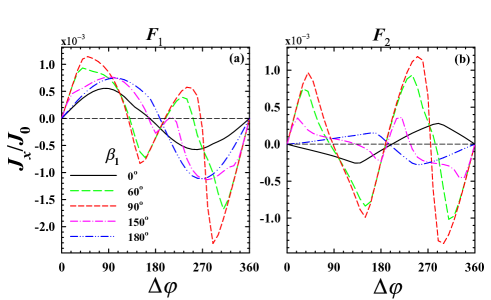
Figure 3: Normalized supercurrent flowing through the ferromagnetic regions vs $\Delta\varphi$. The central $S$ layer has width $d_{S}=\xi_{0}$. We consider several magnetization orientations, $\beta_{1}$ (see legend), inside the $F_{1}$ layer of width $d_{F1}=0.1\xi_{0}$. The magnetization direction of the larger $F_{2}$ layer ($d_{F2}=3.8\xi_{0}$) is strictly along $z$, corresponding to $\beta_{2}=0^{\circ}$.

Figure 3 shows the CPRs at various magnetization directions $\beta_{1}$. The magnetization in $F_{2}$ is fixed along the $z$ direction. The width of the central $S$ layer is now set at $d_{S}=\xi_{0}$, and as stated earlier, its phase has the value $\varphi/2$ to ensure that adjacent superconductors maintain the same phase difference. Examining panel (a), we see that when the relative magnetizations are parallel ($\beta_{1}=0^{\circ}$) or antiparallel ($\beta_{1}=180^{\circ}$), the current exhibits a nearly sinusoidal CPR. For intermediate $\beta_{1}$ leading to noncollinear magnetizations, higher order harmonics appear in the Josephson current. Figure 3(b) reveals that in the wider $F_{2}$ region, collinear orientations result in regular sawtooth-like patterns in the charge current as $\Delta\varphi$ varies. The current in the larger magnet flows in opposite directions depending on whether the relative magnetizations are parallel or antiparallel, in contrast to the narrow $F_{1}$ segment reported in (a). Similarly to what is observed in the narrow $F_{1}$ region, we also find more complicated higher order harmonics in describing the current for misaligned relative magnetizations.

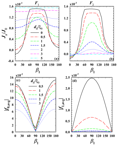
Figure 4: (a) and (b): Normalized Josephson current vs the relative in-plane magnetization angle, $\beta_{1}$ (see Fig. 1). The exchange fields in the two magnets are parallel when $\beta_{2}=0$, and antiparallel when $\beta_{2}=180^{\rm o}$. The magnitude of the exchange field is set to $h=0.1\varepsilon_{F}$. The outer $S$ electrodes have $\Delta\varphi=45^{\circ}$. Five different $S$ widths are considered, as depicted in the legend. Panels (c) and (d) show the average (over the central $S$ region) of the magnitudes of the triplet correlations vs $\beta_{1}$.

In the broader context of layered $F/S$ structures, including ferromagnetic Josephson junctions and spin valves, misalignment of adjacent $F$ layer magnetizations will typically generate equal-spin pairing that is greatest in the orthogonal configurationalidoust_sff ; Karminskaya ; halt_tc ; Fominov_tc . To investigate the supercurrent transport properties when proximity-induced triplet pair correlations are present in $S$$F$$S$$F$$S$ type structures, it is instructive to investigate the sensitivity of $J_{x}$ to relative magnetizations orientation. Therefore in Fig. 4, the Josephson current and triplet correlations are shown in the two ferromagnets as a function of exchange field orientation, $\beta_{1}$. As $\beta_{1}$ sweeps between the parallel ($\beta_{1}=0^{\circ}$) and antiparallel ($\beta_{1}=180^{\circ}$) states, adjacent $S$ electrodes are, as before, maintained at constant phase difference $\varphi/2$. Multiple middle $S$ terminal thicknesses are considered (see legend), with the $d_{S}=0$ curve shown for comparison purposes. As shown in Fig. 4(a) and (b), when magnetic coupling is significant (for $d_{S}\lesssim 2\xi_{0}$) the supercurrent is nonmonotonic and can be highly sensitive to the relative direction of the magnetic moments in the $F$ layers. When the magnets have collinear magnetizations, the Josephson current in $F_{1}$ is often weaker for the parallel configuration compared to the antiparallel configuration, except when there is no central superconductor, or when it is very wide. The orthogonal state ($\beta_{1}=90^{\circ}$) however results in the maximal current flow. Increments in the central electrode thickness can drastically modify the supercurrent signature. Eventually for large enough $d_{S}$, the magnetic coupling is diminished, and variations in $\beta_{2}$ can no longer affect the current flow. The corresponding decoupled $SFS$ junctions then have uniform current flow, that is larger in the narrow $F_{1}$ region (panel (a)), and in $F_{2}$ (panel(b)), becomes negligible due to the larger width.

The emergence of additional harmonics in the current phase relations is often correlated with the generation of triplet correlations that are odd in time halter_trplt or frequency. As we saw previously in Fig. 3, varying the phase difference $\Delta\varphi$, revealed the emergence of additional harmonics as the relative exchange fields went from the parallel ($\beta_{2}=0^{\rm o}$) to orthogonal ($\beta_{2}=90^{\rm o}$) magnetic configuration. To further explore the evolution of triplet pairing correlations with magnetic orientations, in (c) and (d) the spatially averaged triplet amplitudes $|f_{0,{\rm avg}}|$ (with spin projection $m=0$), and $|f_{1,{\rm avg}}|$ (with spin projection $m=\pm 1$) are shown as functions of $\beta_{1}$. These quantities are calculated using the expressions: halter_trplt $f_{0}(x,t)={1}/{2}\sum_{n}(f_{n}^{\uparrow\downarrow}(x)-f_{n}^{\downarrow\uparrow}(x))\zeta_{n}(t)$, and $f_{1}(x,t)={1}/{2}\sum_{n}(f_{n}^{\uparrow\uparrow}(x)+f_{n}^{\downarrow\downarrow}(x))\zeta_{n}(t)$, where we define $\zeta_{n}(t)\equiv\cos(\epsilon_{n}t)-i\sin(\epsilon_{n}t)\tanh({\epsilon_{n}}/{(2T)})$, and $f_{n}^{\sigma\sigma^{\prime}}(x)\equiv u_{n\sigma}(x)v^{\ast}_{n\sigma^{\prime}}(x)$. The summations are in principle over all states. A representative value of $\tilde{t}=6$ is used for the scaled relative time, where $\tilde{t}\equiv\omega_{D}t$. The quantization axis in the regions of interest is aligned along the $z$-direction, however it is straightforward to align it along a different axis that may coincide with the local magnetization direction. halter_gr_tc Comparing Figs. 4(c) and (d), it is evident that the behavior of the triplet amplitudes as a function of $\beta_{1}$ is anticorrelated, with the average $|f_{0}|$ smallest when $|f_{1}|$ peaks at $\beta_{1}=90^{\circ}$. Increasing the $S$ width is shown to reduce the $f_{0}$ amplitudes gradually, however the equal-spin component $f_{1}$ drops much more abruptly to negligible values once $d_{S}$ exceeds $\xi_{0}$. Although not shown, the singlet correlations within $S$ (for all $S$ widths) were found to not exhibit significant sensitivity to changes in $\beta_{1}$. This is clearly in sharp contrast to what is observed for both triplet components. Having discussed now some salient features of the charge currents, we now turn our attention to spin transport and the corresponding equilibrium spin transfer torques within the junction region.

III.2 Spin currents and spin transfer torques

Spin-polarized transport quantities are of paramount importance when studying $S$$F$$S$$F$$S$ type junctions as potential components in spintronics devices. The spin current ${\bm{S}}$ is a local quantity responsible for the change in magnetizations due to the flowing of spin-polarized currents. The main contributor to the equilibrium spin current and corresponding spin-transfer torque $\bm{\tau}$ is the spin-resolved Andreev bound states Zhao , which play the main role in torque sensitivity to variations in $\Delta\varphi$ and $\beta_{1}$. Thus, the STT can be a useful probe of the spin degree of freedom in $S/F$ proximity elements. The current that is generated from the macroscopic phase differences in the $S$ electrodes can become spin-polarizedalidoust_spn ; waintal_1 ; waintal_2 ; zareyan_3 when entering one of the ferromagnet regions. A portion of this spin current can then interact with the other ferromagnet and be absorbed by the local magnetization due to the spin-exchange interactions. wuwu Since we are considering ferromagnets with in-plane magnetic exchange fields, the only spin current that can flow is the out-of-plane component $S_{x}$. This is consistent with the fact that only $\tau_{x}$ can exist in equilibrium when spin currents do not enter or leave the superconducting electrodes.waintal_1

As shown in the Appendix, the method used here to determine $\bm{\tau}$ involves simply calculating the magnetic moment throughout the entire system and then using,

$${\bm{\tau}}=-\frac{2}{\mu_{B}}{\bm{m}}\times{\bm{h}},$$ (10)

where the magnetization components are given in Eqs. (3)-(5). Equivalently, in the steady state, one can use the continuity equation for the spin current [Eq. (21)] to determine the torque transferred by simply evaluating the derivative of the spin current as a function of position:

$${\bm{\tau}}=\frac{\partial{\bm{S}}}{\partial x}.$$ (11)

The net flux of spin current $\Delta S_{x}$ through a certain region bound by points $x_{1}$ and $x_{2}$ is therefore:

$$\Delta S_{x}={\bm{S}}_{x}(x_{2})-{\bm{S}}_{x}(x_{1})=\int^{x_{2}}_{x_{1}}dx{\tau}_{x}=\tau_{x,{\rm tot}}.$$ (12)

In other words, the change in spin current at the interface boundaries ($x=x_{1}$ and $x=x_{2}$) is equivalent to the net torque acting within those boundaries. Either approach, using Eq. (10), or Eq. (11), is sufficient to calculate ${\bm{\tau}}$, as they both yield precisely the same result. In the results that follow, we calculate the torques using Eq. (10), thus avoiding the numerical derivatives that arise when using Eq. (11).

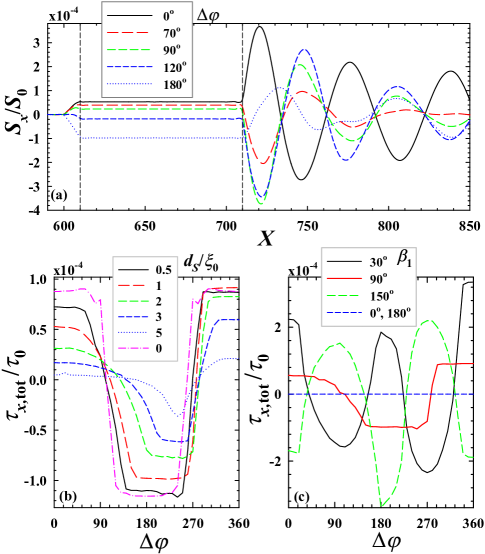
Figure 5: (a) Normalized spin current, $S_{x}$, as a function of normalized position $X$. Several phase differences $\Delta\varphi$ are considered. The interfaces separating each region are denoted by vertical dashed lines. The spin current is conserved in the central $S$ region, where there is no magnetic exchange interaction. (b) Normalized total equilibrium torque, $\tau_{x,{\rm tot}}$, as a function of the superconducting phase difference $\Delta\varphi$ between the outermost $S$ electrodes. A wide range of $d_{S}/\xi_{0}$ ratios are considered (see legend).

We first present in Fig. 5(a) the $x$-component of the local spin current, $S_{x}$, normalized by $S_{0}\equiv-\mu_{B}{\cal N}_{F}\varepsilon_{F}/k_{F}$, where ${\cal N}_{F}$ is the density of states at the Fermi energy. We numerically calculate $S_{x}$ by summing the quasiparticle amplitudes and energies using Eq. (II). Several different phase differences are studied as shown in the legend, and the exchange interactions are orthogonal: ${\bm{h}}_{1}=(0,h_{y1},0)$, and ${\bm{h}}_{2}=(0,0,h_{z2})$. The central $S$ layers is one $\xi_{0}$ wide. The spin current reveals precise spatial behavior of the junction interlayer magnetic coupling, and from Eq. (11), one can deduce the corresponding local behavior of $\tau_{x}$. In $F_{2}$, the oscillating spin currents each have a phase and magnitude that can change, depending on $\Delta\varphi$. Once the spin current enters the $S$ region (bound by the dashed vertical lines), it immediately becomes conserved, whereby there is no transfer of spin angular momentum. Since $\partial S_{x}/\partial x=0$, we have $\tau_{x}=0$ in that region. Within $F_{1}$, the narrow width limits the extent at which $S_{x}$ can vary, and consequently it undergoes a nearly monotonic decline, before vanishing within the superconductor. Since $S_{x}=0$ in the outer $S$ electrodes, the difference $\Delta S_{x}$ over either ferromagnet is determined by the value of $S_{x}$ within the central $S$. Thus, despite drastically different local behavior of $S_{x}$ in each $F$ region, the net flux of spin current through either $F_{1}$ or $F_{2}$ differs only in sign. One can then see that by examining the value of the conserved $S_{x}$ in the central $S$ region, the flux $\Delta S_{x}$ through e.g., $F_{1}$ is largest when $\Delta\varphi=180^{\circ}$, and smallest when $\Delta\varphi=120^{\circ}$. This observation is consistent with (b), where the total torque (normalized by $\tau_{0}\equiv-\mu_{B}{\cal N}_{F}\varepsilon_{F}$) is shown as a function of $\Delta\varphi$. We calculate $\tau_{x,{\rm tot}}$ over the $F_{1}$ region using Eq. (12), although the result for $F_{2}$ is trivially obtained, since within each of the three $s$-wave $S$ electrodes, there can be no flux of spin current. This requires $\tau_{x,{\rm tot}}$ in $F_{1}$ to be the exact opposite in $F_{2}$. As seen in (b), the net torque can be quite sensitive to the phase difference $\Delta\varphi$, which when tuned appropriately, can flip direction or vanish altogether. For comparison, the $d_{S}=0$ case is included, which has symmetric behavior about $\Delta\varphi=180^{\circ}$. For most $S$ layer widths considered, $\tau_{x,{\rm tot}}$ vanishes at $\Delta\varphi\approx 90^{\rm o}$, and $\Delta\varphi\approx 270^{\rm o}$ before reversing direction. Since the middle $S$ terminal has $\varphi_{M}=\varphi/2$, the central $S$ electrode tends to asymmetrically distort the supercurrent about $\Delta\varphi_{R}=180^{\circ}$. Comparing Fig. 2(a) with Fig. 5(b), it is evident that the charge supercurrent $J_{x}$ is not simply correlated with the flux of spin current (or equivalently $\tau_{x,{\rm tot}}$), consistent with previous workwaintal_1 . The coupling between ferromagnets is clearly stronger the thinner the $S$ electrodes, where $\tau_{x,{\rm tot}}$ is larger and tends to change less over a broader range of $\Delta\varphi$, reflecting a tendency for the magnetization to remain fixed in place despite supercurrent variations. Eventually however, for sufficient increments in $\Delta\varphi$, the net torque will abruptly reverse direction.

The proposed $S$$F$$S$$F$$S$ system can be considered as a type of superconducting magnetic torque transistor, where the flow of spin and charge currents are tuned by $\Delta\varphi$. This, in turn, dictates the torques acting on the exchange fields present in the $F$ layers. By minimizing the free energy, waintal_1 it was shown that changes in the supercurrent with respect to relative magnetization orientation results in a torque that changes with $\Delta\varphi$, and vice versa. To underscore the sensitivity of the net torque to the phase and relative magnetic orientations, Fig. 5(c) illustrates $\tau_{x,{\rm tot}}$ as a function $\Delta\varphi$ for a few orientation angles, $\beta_{1}$. When $\bm{m}$ and $\bm{h}$ are collinear, i.e., the two exchange field alignments in the ferromagnets are parallel ($\beta_{1}=0^{\circ}$) or antiparallel ($\beta_{2}=180^{\circ}$) to one another, ${\bm{m}}{\bm{\times}}{\bm{h}}=0$, and hence the net torque is zero (see Eq. (10)). The previous $\beta_{2}=90^{\circ}$ case in (b) is also shown here. For noncollinear magnetizations, a “static” torque even exists in the absence of a supercurrent ($\Delta\varphi=0$). In this case, the effectively inhomogeneous magnetization generates a spin current imbalance and torque that tends to align the magnetizations. When the magnetizations are misaligned, the supercurrent can change both the direction and amplitude of the torquebuzdin_sfsfs . In many cases, this effect can be attributed to the torque that the equal-spin triplet component of the supercurrent (possessing net spin along the spin quantization axis) exerts on the magnetization and tends to rotate it. As we clearly see from the results presented in Fig. 5(c), for thin central superconductors with $d_{S}\lesssim\xi_{0}$, this effect can be quite sensitive to the multiple superconducting phase differences.

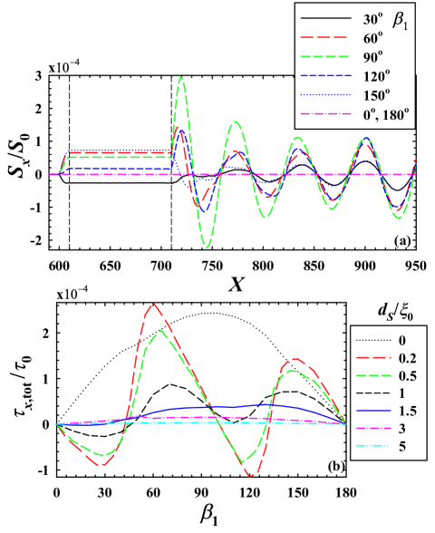
Figure 6: (a) The $x$ component of the spin current $S_{x}$ flowing throughout a segment of the $S$$F$$S$$F$$S$ junction, as a function of position $X$. The magnetic exchange orientation in $F_{1}$ is varied according to ${\bm{h}}_{1}=h(0,\sin\beta_{1},\cos\beta_{1})$, while in $F_{2}$ we have:, ${\bm{h}}_{2}=(0,0,h)$. The intermediate $S$ width corresponds to $d_{S}/\xi_{0}=1$. The legend identifies the different angles $\beta_{1}$ used. A current is established via a phase difference of $\Delta\varphi=45^{\circ}$ between the outer $S$ layers. Spatial variations in $S_{x}$, are responsible for any torques present in the system. In (b) the total torque, $\tau_{x,\rm tot}$, is plotted as a function of $\beta_{1}$. The $d_{S}=0$ reference case is multiplied by a constant factor for comparison purposes. Each curve corresponds to a different $d_{S}$ as identified in the legend.

To investigate further the behavior of the local spin transport, and total torque when varying the ferromagnet orientation angle $\beta_{1}$, the spatial behavior of spin current throughout the system is shown in Fig. 6(a). The angle $\beta_{1}$ describes the rotation of the in-plane magnetic exchange in $F_{1}$: ${\bm{h}}_{1}=h(0,\sin\beta_{1},\cos\beta_{1})$. The magnetic exchange field direction in $F_{2}$ does not vary and is directed along $z$: ${\bm{h}}_{2}=(0,0,h)$. Control of the free-layer magnetization by an external magnetic field has experimentally been demonstrated in $S/F$ spin valves ilya . The rotation angle can also be manipulated by STT switching.Bauer_nat ; brataas_nat We see that in the $S$ region, $S_{x}$ is constant for all angles $\beta_{1}$, consistent with the spin-torque conservation law [Eq. (11)] which states that any spatial variations of the spin current must generate a torque. The torque thus vanishes in the $S$ region, as it should. The $F_{2}$ region again exhibits a spatially modulating spin current whose behavior is highly sensitive to the particular orientation angle $\beta_{1}$. The most rapid changes in the oscillating $S_{x}$ tends to occur within this ferromagnet near the interface with a superconductor. We also see that the spin current at the interfaces between the ferromagnets and the central $S$ (dashed vertical lines) varies non-monotonically, changing sign at $\beta_{1}=30^{\circ}$, or vanishing altogether when the magnetizations are collinear ($\beta_{1}=0^{\circ}$, or $\beta_{1}=180^{\circ}$). These observations are consistent with Fig. 6(b), where the total torque $\tau_{x,{\rm tot}}$ is shown as a function of orientation angle $\beta_{1}$ for several $S$ widths. We see that $\tau_{x,{\rm tot}}$ vanishes entirely when the two ferromagnets have collinear magnetizations, corresponding to parallel ($\beta_{1}=0^{\circ}$) or antiparallel ($\beta_{1}=180^{\circ}$) configurations. The total torque also has the expected behavior when there is no middle $S$ terminal ($d_{S}=0$), peaking when $\beta_{1}\approx 90^{\circ}$, corresponding to the situation where the torque has the greatest tendency to align the magnetic moments. Including a central $S$ layer is seen to introduce a nontrivial oscillatory behavior in $\tau_{x,{\rm tot}}$ that can cause it to vanish (or change direction) multiple times when spanning the full $\beta_{1}$ range. In effect, the angle $\beta_{1}$ that was previously responsible for the largest total torque (when $d_{S}=0$) is now the angle at which there is negligible total torque within the $F$ layers. Increasing the $S$ thickness of course reduces the ferromagnetic coupling and hence reduces the magnitude of the mutual torques. The misalignment angle where the maximum torque is exerted, $\beta^{*}_{1}$, clearly shifts from near the orthogonal configuration ($\beta^{*}_{1}\approx 90^{\rm o}$) when $d_{S}=0$ towards intermediate magnetic configurations corresponding to $60^{\circ}\lesssim\beta_{1}\lesssim 70^{\circ}$, for $d_{S}\lesssim\xi_{0}$.

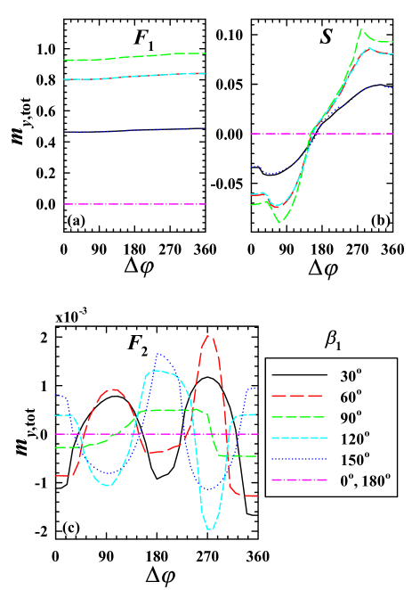
Figure 7: The normalized $y$ component of the total magnetization $m_{y,{\rm tot}}$, as a function of phase, $\Delta\varphi$, within the $S$$F$$S$$F$$S$ system. is shown for a few in-plane exchange field orientations, $\beta_{1}$ (see legend). The $F_{1}$ region has a thickness corresponding to $d_{F1}/\xi_{0}=0.1$, $F_{2}$ has $d_{F2}/\xi_{0}=3.8$, and the central layer is one coherence length wide, i.e., $d_{S}/\xi_{0}=1$. The exchange field has magnitude $h=0.1$. Each panel (a)-(c) depicts a different region where the net magnetization is calculated. The leakage of magnetism into the central $S$ region [panel (b)] is clearly visible.

To examine the previous behavior of the total STT from a different perspective, it is beneficial to recall the simple expression, Eq. (10), which shows that for a given exchange field, the torque arises entirely from the magnetization, ${\bm{m}}(x)$. Thus, it is insightful to study the details of ${\bm{m}}(x)$, which gives a measure of the spin polarization in the system responsible for generating the local spin currents. The out-of-plane torque is due to both in-plane components of the magnetization: $\tau_{x}(x)=-(2/\mu_{B})[m_{y}(x)h_{z}(x)-h_{y}(x)m_{z}(x)]$, which clearly vanishes outside of the ferromagnet regions where ${\bm{h}}_{i}=0$. The exchange field in the $F_{1}$ region varies in the $yz$ plane, while in $F_{2}$, the only nonzero component to the exchange field is $h_{z}$, so that we have simply, $\tau_{x}(x)=-(2/\mu_{B})h_{z}(x)m_{y}(x)$. Thus for a mutual torque to exist in the ferromagnets, a $y$-polarized magnetization in $F_{1}$ must propagate through the central $S$ electrode and into the $F_{2}$ layer, generating a spin-imbalance. In Fig. 7(a-c), we illustrate the total magnetization, $m_{y,{\rm tot}}$, in each region as a function of $\Delta\varphi$. Here we define the quantity $m_{y,{\rm tot}}$ as the $y$-component of the magnetization spatially integrated over each of the three junction regions of interest, and normalized by $m_{0}\equiv-\mu_{B}{\cal N}_{F}$. Using this normalization, the bulk value of the magnetization is equivalent to the exchange field value of $h/\varepsilon_{F}=0.1$. The thicknesses of the $F_{1}$, $F_{2}$, and $S$ layers are given by $d_{F1}/\xi_{0}=0.1$, $d_{F2}/\xi_{0}=3.8$, and $d_{S}/\xi_{0}=1$, respectively. It is evident that for a wide range of $\Delta\varphi$, a net magnetization exists in each junction region, other than when $\beta_{1}$ corresponds to relative collinear magnetizations (${\bm{h}}_{1}$ directed along $z$). In panel (a), $m_{y,{\rm tot}}$ is approximately constant for each $\beta_{1}$, and the overlapping curves at $\beta_{1}=30^{\circ},150^{\circ}$ reflect the symmetry about $\beta_{1}=90^{\circ}$, where the net magnetization is greatest. Also, the net magnetization in $F_{1}$ is positive for the range of $\beta_{1}$ shown, since the magnetic exchange interaction in the $y$ direction is $h_{1,y}=h\sin\beta_{1}$. Due to proximity effects, there is an intrinsic net magnetization in the superconductor that is present even in the absence of current flow. As shown in panel (b), the total induced magnetization in the superconductor is finite at $\Delta\varphi=0^{\circ}$ and vanishes at $\Delta\varphi\approx 180^{\circ}$, where it switches direction. Finally, in Fig. 7(c) the contribution from the magnetization to the total torque observed in Fig. 5 is evident, where the total magnetization in the wider $F_{2}$ region exhibits the same dependence on $\Delta\varphi$ as $\tau_{x,{\rm tot}}$, differing only in sign.

IV Conclusions

In conclusion, we have presented a detailed microscopic study of the charge and spin supercurrents that can exist in $S$$F$$S$$F$$S$ types of Josephson junction hybrids. The local magnetization profiles were then calculated and employed for determining the equilibrium spin transfer torques. We also studied the associated spin-triplet correlations that arise in these hybrids. This was accomplished by solving the BdG equations over a broad range of geometrical and material parameters. Our investigations revealed how to manipulate and generate supercurrents with higher order harmonics by varying the macroscopic phases in the superconducting electrodes, or the relative exchange field orientations. Utilizing the spin conservation law, we calculated the spin transfer torque in these systems, revealing a number of experimentally viable ways in which the magnetization can be controlled in a prescribed fashion. Our results demonstrate that, depending on the parameters considered, these types of ballistic systems can support supercurrents that can be tuned to contain primarily the first or second harmonics in the current-phase relations. We studied the $\pi$-$2\pi$ harmonic crossovers and determined the experimentally desirable conditions in which to reveal the second harmonic supercurrents in these systems. We also showed that the equilibrium spin transfer torques can be well controlled by simply modulating the macroscopic phases of the three $S$ electrodes in addition to the other system parameters such as the sizes of the ferromagnets and central superconductor electrodes, or the relative magnetization alignments. These findings are suggestive of a phase-tunable superconducting transistor based on STT switching.

Appendix A Numerical procedure for solving the BdG equations

The numerical procedure used in calculating the spin and charge currents involves first expandingklaus the quasiparticle amplitudes in terms of a complete set of $N$ basis functions:

$$\psi_{n}(x)=\sqrt{\frac{2}{d}}\sum_{q=0}^{N}\sin({k_{q}x})\hat{\psi}_{q}(k_{q}),$$ (13)

where we define $\psi_{n}(x)=(u_{n\uparrow}(x),u_{n\downarrow}(x),v_{n\uparrow}(x),v_{n\downarrow}(x))$, and $\hat{\psi}_{q}=(\hat{u}_{q\uparrow},\hat{u}_{q\downarrow},\hat{v}_{q\uparrow},\hat{v}_{q\downarrow})$. The wavevector $k_{q}=q\pi/d$ is discretized in terms of the system width $d$, taken to be large enough so that the results become independent of $d$. The next step involves Fourier transforming the real-space BdG equations (Eq. (1)), resulting in the following set of coupled equations in momentum space:

$$\begin{pmatrix}\hat{H}_{0}-\hat{h}_{z}&-\hat{h}_{x}+i\hat{h}_{y}&0&\hat{\Delta}\\ -\hat{h}_{x}-i\hat{h}_{y}&\hat{H}_{0}+h_{z}&\hat{\Delta}&0\\ 0&{\hat{\Delta}}^{*}&-(\hat{H}_{0}-\hat{h}_{z})&-\hat{h}_{x}-i\hat{h}_{y}\\ {\hat{\Delta}}^{*}&0&-\hat{h}_{x}+i\hat{h}_{y}&-(\hat{H}_{0}+\hat{h}_{z})\\ \end{pmatrix}\begin{pmatrix}\hat{u}_{\uparrow}\\ \hat{u}_{\downarrow}\\ \hat{v}_{\uparrow}\\ \hat{v}_{\downarrow}\end{pmatrix}=\epsilon_{n}\begin{pmatrix}\hat{u}_{\uparrow}\\ \hat{u}_{\downarrow}\\ \hat{v}_{\uparrow}\\ \hat{v}_{\downarrow}\end{pmatrix}.$$ (14)

Here we have defined $\hat{u}_{\sigma}=(\hat{u}_{1\sigma},\hat{u}_{2\sigma},\ldots,\hat{u}_{N\sigma})$, $\hat{v}_{\sigma}=(\hat{v}_{1\sigma},\hat{v}_{2\sigma},\ldots,\hat{v}_{N\sigma})$, and the matrix elements,

$$\hat{H}_{0}(q,q^{\prime}) =\frac{2}{d}\int_{0}^{d}dx\left(\frac{k_{q}^{2}}{2m}+\epsilon_{\perp}-\mu\right)\sin(k_{q}x)\sin(k_{q^{\prime}}x),$$ (15)

$$\hat{\Delta}({q,q^{\prime}}) =\frac{2}{d}\int_{0}^{d}dx\Delta(x)\sin(k_{q}x)\sin(k_{q^{\prime}}x),$$ (16)

$$\hat{h}_{i}({q,q^{\prime}}) =\frac{2}{d}\int_{0}^{d}dx\,h_{i}(x)\sin(k_{q}x)\sin(k_{q^{\prime}}x),\quad i=x,y,z.$$ (17)

Our numerical procedure for calculating the supercurrent involves assuming a constant amplitude and phase for the pair potential in each $S$ layer, thus providing the physically necessary source or sink of current, via the external electrodes. We then expand the pair potential via Eq. (16). Similarly the exchange field and free particle Hamiltonian are expanded using Eq. (17) and Eq. (15) respectively. We then find the quasiparticle energies and amplitudes by diagonalizing the resultant momentum-space matrix (Eq. (14)). Once the momentum-space wavefunctions and energies are found, they are transformed back into real-space via Eq. (13), and the currents and magnetic moments are calculated as described in Sec. II.

As mentioned above, the current source arises from the non self-consistent region where we take $\Delta(x)$ to be a piecewise constant with prescribed macroscopic phases in the $S$ electrodes. The widths of the two outer $S$ terminals are sufficiently large ($d_{S}\gg\xi_{0}$) so that the system boundaries have a negligible influence on the results. By taking the divergence of the current in Eq. (6) and using the BdG equations (Eq. (1)), we find,

$$\frac{\partial J_{x}(x)}{\partial x}=2e{\rm Im}\left\{\Delta({x})\sum_{n}\left[u_{n\uparrow}^{*}v_{n\downarrow}+u_{n\downarrow}^{*}v_{n\uparrow}\right]\ \tanh\left(\frac{\epsilon_{n}}{2T}\right)\right\},$$ (18)

where the terms in the summation constitute the usual self-consistency equation Gennes for $\Delta(x)$. Thus, only when self-consistency in $\Delta({x})$ is achieved, does the right hand side of Eq. (18) vanish, and current is conserved. If the self-consistency condition is not strictly satisfied, the terms on the right act effectively as sources of current, except of course within the ferromagnet regions, where $\Delta({x})=0$.

Appendix B Spin current and spin transfer torque

The spin current can be found by using the Heisenberg picture. First we determine the time evolution of the spin density, ${\bm{\eta}}({x})$,

$$\frac{\partial}{\partial t}\langle{\bm{\eta}}({x})\rangle=i\Big{\langle}[{\cal H},{\bm{\eta}}({x})]\Big{\rangle},$$ (19)

where the effective BCS Hamiltonian ${\cal H}$ is written,

$${\cal H}= \int dx\Bigl{\{}\psi^{\dagger}({x})[{\cal H}_{0}({x})-{\bm{h}}({x})\cdot{\bm{\sigma}}]\psi({x})$$

$$+\Delta({x})\psi^{\dagger}_{\uparrow}({x})\psi^{\dagger}_{\downarrow}({x})+\Delta^{*}({x})\psi_{\downarrow}({x})\psi_{\uparrow}({x})\Bigr{\}}.$$ (20)

Here we define, $\psi({x})=(\psi_{\uparrow}({x}),\psi_{\downarrow}({x}))^{\mathbb{T}}$, and the spin density operator ${\bm{\eta}}({x})$: ${\bm{\eta}}({x})=\psi^{\dagger}({x}){\mbox{\boldmath$\sigma$}}\psi({x})$. Inserting the Hamiltonian (Eq. (B)), into Eq. (19), we end up with the spin continuity equation:

$$\frac{\partial}{\partial t}\langle{\bm{\eta}}({x})\rangle+\frac{\partial}{\partial x}{\bm{S}}({x}) ={\bm{\tau}}({x}),$$ (21)

where the spin transfer torque ${\bm{\tau}}$ is written in terms of the expectation value, ${\bm{\tau}}(x)=2\langle\psi^{\dagger}({x})[{\bm{\sigma}}{\bm{\times}}{\bm{h}}]\psi({x})\rangle$. Using the fact that the spin density is simply related to the magnetization ${\bm{m}}$ via ${\bm{m}}({x})=-\mu_{B}\,\langle{\bm{\eta}}({x})\rangle$, we end up with Eq. (10). Similarly, the spin current ${\bm{S}}$ is given by:

$${\bm{S}}({x}) =-\frac{i}{2m}\Bigg{\langle}\psi^{\dagger}({x}){\bm{\sigma}}\left({\frac{\partial}{\partial x}}\psi({x})\right)-\left({\frac{\partial}{\partial x}}\psi^{\dagger}({x})\right){\bm{\sigma}}\psi({x})\Bigg{\rangle}.$$ (22)

Lastly, we insert the Bogolibuov transformations, $\psi_{\uparrow}({x})=\sum_{n}(u_{n\uparrow}({x})\gamma_{n}-v^{*}_{n\uparrow}({x})\gamma_{n}^{\dagger})$, and $\psi_{\downarrow}({x})=\sum_{n}(u_{n\downarrow}({x})\gamma_{n}+v^{*}_{n\downarrow}({x})\gamma_{n}^{\dagger})$, and use conventional rules for the thermal averages: $\langle\gamma_{n}^{\dagger}\gamma_{m}\rangle=\delta_{nm}f_{n}$, $\langle\gamma_{m}\gamma^{\dagger}_{n}\rangle=\delta_{nm}(1-f_{n})$, and $\langle\gamma_{n}\gamma_{m}\rangle=0$, to arrive at Eqs. (II)-(II). Note that ${S}_{\sigma}(x)$ represents the spin current flow along the $x$ direction in configuration-space, with indices $\sigma=x,y,z$ in spin-space.

References

- (1) F.S. Bergeret, A.F. Volkov, K.B. Efetov, Rev. Mod. Phys. 77, 1321 (2005).
- (2) M. Eschrig, Phys. Today 64, 43 (2011).
- (3) K.B. Efetov, I.A.Garifullin, A.F.Volkov,K.Westerholt, Magnetic Heterostructures. Advances and Perspectives in Spin structures and Spin transport. ed. by H. Zabel, S.D. Bader, Series. Springer Tracts in Modern Physics, vol 227 (Springer, New York, 2007), P. 252
- (4) A.A. Golubov, MYu. Kupriyanov, E. Ilichev, Rev. Mod. Phys. 76, 411 (2004).
- (5) A. Buzdin, Rev. Mod. Phys. 77, 935 (2005).
- (6) K. Sun and N. Shah, Phys. Rev. B 91, 144508 (2015).
- (7) M. Alidoust and K. Halterman, Phys. Rev. B89, 195111 (2014).
- (8) L. Trifunovic, Z. Popovic, Z. Radovic, Phys. Rev. B 84, 064511 (2011).
- (9) X. Waintal, P.W. Brouwer, Phys. Rev. B 65, 054407 (2002).
- (10) J. Zhu, I.N. Krivorotov, K. Halterman, O.T. Valls, Phys. Rev. Lett. 105, 207002 (2010).
- (11) K. Halterman, O.T. Valls, and M. Alidoust, Phys. Rev. Lett. 111 046602 (2013).
- (12) M. Eschrig, J. Kopu, A. Konstandin, J.C. Cuevas, M. Fogelstrom, G. Schon, Advances in Solid State Physics, 44, 533 (2004).
- (13) M. Eschrig, T. Lofwander, T. Champel, J. C. Cuevas, J. Kopu, Gerd Schon, J. Low Temp. Phys. 147, 457, (2007).
- (14) K. Halterman, P.H. Barsic, O.T. Valls, Phys. Rev. Lett. 99, 127002 (2007).
- (15) M. Alidoust and K. Halterman, J. Appl. Phys. 117, 123906 (2015).
- (16) F. Giazotto, J. T. Peltonen, M. Meschke, and J. P. Pekola,Nat. Phys. 6, 254 (2010).
- (17) P. Spathis, S. Biswas, S. Roddaro, L. Sorba, F. Giazotto, and F. Beltram, Nanotechnology 22, 105201 (2011).
- (18) M. Alidoust, K. Halterman, and J. Linder, Phys. Rev. B 88, 075435 (2013).
- (19) J.C. Slonczewski, J. Magn. Magn. Mat. 159 (1996).
- (20) L. Berger, Phys. Rev. B 54 9353 (1996).
- (21) J. Linder and J.W.A. Robinson, Nat. Phys. 11, 307 (2015).
- (22) I. Zutic, J. Fabian, and S. Das Sarma, Rev. Mod. Phys. 76, 323 (2004).
- (23) A. Fert, Rev. Mod. Phys. 80, 1517 (2008).
- (24) A. Brataas, A.D. Kent, and H. Ohno, Nat. Mat. 11, 372 (2012).
- (25) G.E.W. Bauer, E. Saitoh, and B.J. van Wees, Nat. Mat. 11, 391 (2012).
- (26) N. Pugach, and A. Buzdin, Appl. Phys. Lett. 101, 242602 (2012).
- (27) V.V. Ryazanov, V.V. Bolginov, D.S. Sobanin, I.V. Vernik, S.K. Tolpygo, A.M. Kadin, O.A. Mukhanov, Physics Procedia 36, 35 (2012).
- (28) I.T. Larkin, V.V. Bolginov, V.S. Stolyarov, V.V. Ryazanov, I.V. Vernik, S.K.T. and O.A. Mukhanov, Appl. Phys. Lett. 100, 222601 (2012).
- (29) S.V. Bakurskiy, N.V. Klenov, I.I. Soloviev, V.V. Bolginov, V.V. Ryazanov, I.V. Vernik, O.A. Mukhanov, M.Yu. Kupriyanov and A.A. Golubov ,Appl. Phys. Lett. 102, 192603 (2013).
- (30) I.V. Vernik, V.V. Bolginov, S.V. Bakurskiy, A.A. Golubov, M.Y. Kupriyanov, V.V. Ryazanov, and O.A. Mukhanov ,IEEE Tran. Appl. Supercond. 23 1701208 (2013).
- (31) S.V. Bakurskiy, N.V. Klenov, I.I. Soloviev, M.Yu. Kupriyanov, and A.A. Golubov Phys. Rev. B 88, 144519 (2013).
- (32) X. Waintal, P.W. Brouwer, Phys. Rev. B 63, 220407 (2001).
- (33) E. Zhao and J.A. Sauls, Phys. Rev. B78, 174511 (2008).
- (34) M. Alidoust, J. Linder, G. Rashedi, T. Yokoyama, and A. Sodbo, Phys. Rev. B81, 014512 (2010).
- (35) A. Pal, Z.H. Barber, J.W.A. Robinson and M.G. Blamire, Nat. Comm. 5, 3340 (2014).
- (36) M. Bozovic, and Z. Radovic, Phys. Rev. B71, 229901 (2005).
- (37) Z. Radovic, N. Lazarides, and N. Flytzanis, Phys. Rev. B68, 014501 (2003).
- (38) C.W.J. Beenakker, Phys. Rev. Lett. 97, 067007 (2006).
- (39) M.J.M. de Jong, C.W.J. Beenakker, Phys. Rev. Lett. 74, 1657 (1995); C.W.J. Beenakker, Lect. Notes Phys. 667, 131 (2005).
- (40) A. Freyn, B. Doucot, D. Feinberg, and R. Mélin, Phys. Rev. Lett. 106, 257005 (2011).
- (41) V.C.Y. Chang and C.S. Chu, Phys. Rev. B55, 6004 (1997).
- (42) D. Averin and A. Bardas, Phys. Rev. Lett. 75, 1831 (1995).
- (43) Z. Radovic, L. Dobrosavljevic-Grujic, and B. Vujicic, Phys. Rev. B 63, 214512 (2001); T. T. Heikkila, F. K. Wilhelm, and G. Schon, Europhys. Lett. 51, 434 (2000).
- (44) J. J. A. Baselmans, T. T. Heikkila, B. J. van Wees, and T. M. Klapwijk, Phys. Rev. Lett. 89, 207002 (2002).
- (45) V.V. Ryazanov, V.A. Oboznov, A.Yu. Rusanov, A.V. Veretennikov, A.A. Golubov, and J. Aarts, Phys. Rev. Lett. 86, 2427 (2001).
- (46) A. Buzdin, Phys. Rev. B72, 100501(R) (2005); M. Houzet, V. Vinokur, and F. Pistolesi, Phys. Rev. B72, 220506(R) (2005).
- (47) G. Mohammadkhani and M. Zareyan, Phys. Rev. B 73, 134503 (2006).
- (48) J. Linder and K. Halterman, Phys. Rev. B90 , 104502 (2014).
- (49) P.G. deGennes, Superconductivity of Metals and Alloys (Benjamin, New York, 1966).
- (50) K. Halterman and O.T. Valls, Phys. Rev. B65, 014509 (2002).
- (51) M.A. Sillanpää, T.T. Heikkila, R.K. Lindell, and P.J. Hakonen, Europhys Lett 56, 590 (2001).
- (52) K. Halterman and O.T. Valls, Phys. Rev. B 65, 014509 (2002).
- (53) F. S. Bergeret, A. F. Volkov, and K. B. Efetov, Europhys. Lett., 66 111 (2004).
- (54) K. Halterman and O.T. Valls, Phys. Rev. B80, 104502 (2009).
- (55) C.-T. Wu, O. T. Valls, K. Halterman, Phys. Rev. B 86, 184517 (2012).
- (56) K.K. Likharev, Rev. Mod. Phys. 51, 101 (1979).
- (57) B.D. Josephson, Phys. Lett. 1 251 (1962).
- (58) O. Šipr and B.L. Györffy, J. Phys. Condens. Matter 8, 169 (1996).
- (59) M. Alidoust, K. Halterman, and J. Linder, Phys. Rev. B89, 054508 (2014).
- (60) T. Yu. Karminskaya, A. A. Golubov, and M. Yu. Kupriyanov, Phys. Rev. B84, 064531 (2011).
- (61) C.-T. Wu O.T. Valls, and K. Halterman, Phys. Rev. B 86, 014523 (2012).
- (62) Y.V. Fominov, A. Golubov, T. Karminskaya, M. Kupriyanov, R. G. Deminov, and L. R. Tagirov, JETP Lett. 91, 308 (2010).
- (63) Z. Shomali, M. Zareyan, and W. Belzig, New J. Phys. 13, 083033 (2011).
- (64) C.-T. Wu, O.T. Valls, and K. Halterman, Phys. Rev. B 90, 054523 (2014).
- (65) A. A. Jara, C. Safranski, I. N. Krivorotov, C.-T. Wu, A. N. Malmi-Kakkada, O. T. Valls, and K. Halterman, Phys. Rev. B89, 184502 (2014).