Bayesian Estimation of the Kumaraswamy Inverse Weibull Distribution

Abstract

The Kumaraswamy Inverse Weibull distribution has the ability to model failure rates that have unimodal shapes and are quite common in reliability and biological studies. The three-parameter Kumaraswamy Inverse Weibull distribution with decreasing and unimodal failure rate is introduced. We provide a comprehensive treatment of the mathematical properties of the Kumaraswany Inverse Weibull distribution and derive expressions for its moment generating function and the $r$-th generalized moment. Some properties of the model with some graphs of density and hazard function are discussed. We also discuss a Bayesian approach for this distribution and an application was made for a real data set.

Keywords: Kumaraswamy distribution, Weibull distribution, Survival, Bayesian analysis.

1 Introduction

In this paper we propose a new probability distribution to handle the problem of survival data. Motivated by research developed in recent years, we introduce the Kumaraswany Inverse Weibull distribution that includes several well known distributions used in survival analysis.

Recently, many authors have proposed new classes of distributions, which are modifications of distribution functions which provide hazard ratios contemplating various shapes. We can cite for example the Weibull exponential (Mudholkar et al.,, 1995), which has also the hazard rate function with a unimodal form, (see also Xie and Lai, (1996)). Carrasco et al., (2008) proposed a four-parameter distribution denoted generalized modified Weibull (GMW) distribution, Gusmão et al., (2011) introduced and studied the tri-parametric inverse Weibull generalized distribution that possesses failure rate with unimodal, increasing and decreasing forms. Pescim et al., (2010) proposed a distribution with four parameters, called beta generalized half normal distribution.

Underexplored in the literature and rarely used by statisticians, the Kumaraswamy distribution (Kumaraswamy,, 1980) has a domain in the real interval $(0,1)$. This property turns the Kumaraswamy distribution a natural candidate to combine with other distributions to produce a more general one. Its cumulative distribution function (cdf) is given by,

$$F\left(x;a,b\right)=1-\left[1-x^{a}\right]^{b},$$ (1)

and its probability density function (pdf) is given by,

$$f\left(x;a,b\right)=abx^{a-1}\left[1-x^{a}\right]^{b-1},~{}0<x<1,$$

where $a>0$ and $b>0$. This density can be unimodal, increasing, decreasing or constant.

Recently, Cordeiro and de Castro, (2011) proposed to use the Kumaraswamy to generalize other distributions. Considering that a random variable $X$ has distribution $G$, they suggest to apply the Kumarasawamy distribution to $G(x)$. Note that, since $0<G(x)<1$ for any distribution function $G$, then evaluating equation (1) at $G(x)$ we obtain,

$$F_{G}(x;a,b)=1-[1-G(x)^{a}]^{b}.$$ (2)

where $F_{G}$ is the cdf of the generalized Kumaraswamy-$G$ distribution. Based on these ideas, we consider the Inverse Weibull Distribution as a candidate for $G$, using Equation (2). Then, performing some adjustments and mathematical manipulations, we obtain the Kumaraswamy inverse Weibull (Kum-IW) distribution.

The rest of the paper is organized as follows. In Section 2, we develop the Kum-IW distribution. Section 3 is devoted to describe basic properties of the distribution. Inference procedures via maximum likelihood and Bayesian approaches are presented in Section 4. Section 5 is devoted to analyze a real data set and in Section 6 we present some conclusions of this work.

2 Kumaraswamy inverse Weibull distribution

Let $T$ a random variable with inverse Weibull distribution. Then its cdf can be written as,

$$G(t)=\exp\left[-\left(\frac{\alpha}{t}\right)^{\beta}\right],\quad t>0,$$ (3)

where $\alpha>0$, $\beta>0$, and its pdf is given by,

$$g(t)=\beta\alpha^{\beta}t^{-\left(\beta+1\right)}\exp\left[-\left(\frac{\alpha}{t}\right)^{\beta}\right].$$

Inserting the $G$ function of Equation (3) in Equation (2) it follows that,

$$F_{G}(t;a,b,\alpha,\beta)=1-\left\{1-\exp\left[-a\left(\frac{\alpha}{t}\right)^{\beta}\right]\right\}^{b}.$$ (4)

We note that the parameters $a$ and $\alpha$ in (4) are not identifiable and we adopt the reparameterization $c=\alpha a^{1/\beta}$ so that the Kum-IW cdf is rewritten as,

$$F_{G}(t;b,c,\beta)=1-\left\{1-\exp\left[-\left(\frac{c}{t}\right)^{\beta}\right]\right\}^{b},$$ (5)

where $b>0$ and $c>0$ are the shape and scale paremeters respectively. Accordingly, the Kum-IW pdf is now given by,

$$f_{G}(t;b,c,\beta)=\beta bc^{\beta}t^{-\left(\beta+1\right)}\exp\left[-\left(\frac{c}{t}\right)^{\beta}\right]\left\{1-\exp\left[-\left(\frac{c}{t}\right)^{\beta}\right]\right\}^{b-1}.$$ (6)

It can be easily seen that when $b=1$ we obtain the pdf of the Inverse Weibull (IW) distrbution given by,

$$g(t)=\beta\alpha^{\beta}t^{-\left(\beta+1\right)}\exp\left[-\left(\frac{\alpha}{t}\right)^{\beta}\right].$$

Finally, the corresponding survival and hazard functions are respectively given by,

$$S_{G}(t;b,c,\beta)=\left\{1-\exp\left[-\left(\frac{c}{t}\right)^{\beta}\right]\right\}^{b}\quad\mbox{and}\quad h_{G}(t;b,c,\beta)=\frac{\beta bc^{\beta}t^{-\left(\beta+1\right)}\exp\left[-\left(\frac{c}{t}\right)^{\beta}\right]}{1-\exp\left[-\left(\frac{c}{t}\right)^{\beta}\right]}.$$

while the quantile function, $Q(u)$, of the Kum-IW distribution is given by,

$$Q(u)=F^{-1}(u;b,c,\beta)=c(-\log(1-(1-u)^{\frac{1}{b}}))^{-{\frac{1}{\beta}}}$$

2.1 Some special classes of the Kum-IW

The following well known and new distributions are special sub-classes of the Kum-IW distribution.

• Kumaraswamy inverse Rayleigh distribution (Kum-IR)

  If $\beta=2$, the Kum-IW distribution reduces to the Kumaraswamy inverse Rayleigh distribution (Kum-IR). Then, with $\beta=2$ the density function of Kum-IW is expressed by:

  $$F_{G}(t;b,c)=1-\left\{1-\exp\left[-\left(\frac{c}{t}\right)^{2}\right]\right\}^{b},$$

  where $b>0$ is the shape parameter, and $c>0$ is the scale parameter. Hence, the KiR distribution has two parameters, and its pdf is given by

  $$f_{G}(t;b,c)=2bc^{2}t^{-3}\exp\left[-\left(\frac{c}{t}\right)^{2}\right]\left\{1-\exp\left[-\left(\frac{c}{t}\right)^{2}\right]\right\}^{b-1}.$$

  The corresponding survival and hazard functions are given respectively by,

  $$S_{G}(t;b,c)=\left\{1-\exp\left[-\left(\frac{c}{t}\right)^{2}\right]\right\}^{b}~{}~{}~{}~{}\textnormal{and}~{}~{}~{}~{}h_{G}(t;b,c)=\frac{2bc^{2}t^{-3}\exp\left[-\left(\frac{c}{t}\right)^{2}\right]}{1-\exp\left[-\left(\frac{c}{t}\right)^{2}\right]}.$$

• Inverse Rayleigh distribution (IR)

  If $\beta=2$ and $b=1$, the Kum-IW distribution reduces to the inverse Rayleigh distribution (Kum-IR). Then, with $\beta=2$ and $b=1$ the density function of Kum-IW is expressed by:

  $$G(t)=\exp\left[-\left(\frac{\alpha}{t}\right)^{2}\right],\quad t>0,$$

  where $\alpha>0$, and its pdf is

  $$g(t)=2\alpha^{2}t^{-3}\exp\left[-\left(\frac{\alpha}{t}\right)^{2}\right].$$

• Kumaraswamy inverse Exponential distribution (Kum-IE)

  If $\beta=1$, the Kum-IW distribution reduces to the Kumaraswamy inverse Exponential distribution (Kum-IE). Then, with $\beta=1$ the density function of Kum-IW is expressed by:

  $$F_{G}(t;b,c)=1-\left\{1-\exp\left[-\left(\frac{c}{t}\right)\right]\right\}^{b},$$

  where $b>0$ is the shape parameter, and $c>0$ is the scale parameter. Hence, the KIE distribution has two parameters, and its pdf is given by

  $$f_{G}(t;b,c)=bct^{-2}\exp\left[-\left(\frac{c}{t}\right)\right]\left\{1-\exp\left[-\left(\frac{c}{t}\right)\right]\right\}^{b-1}.$$

  The corresponding survival and hazard functions are respectively

  $$S_{G}(t;b,c)=\left\{1-\exp\left[-\left(\frac{c}{t}\right)\right]\right\}^{b}~{}~{}~{}~{}\textnormal{and}~{}~{}~{}~{}h_{G}(t;b,c)=\frac{bct^{-2}\exp\left[-\left(\frac{c}{t}\right)\right]}{1-\exp\left[-\left(\frac{c}{t}\right)\right]}.$$

• Inverse Exponential distribution (IE)

  If $\beta=1$ and $b=1$, the Kum-IW distribution reduces to the Inverse Exponential distribution (IE). Then, with $\beta=1$ and $b=1$ the density function of Kum-IW is expressed by:

  $$G(t)=\exp\left[-\left(\frac{\lambda}{t}\right)\right],\quad t>0,$$

  where $\lambda>0$ and its pdf is

  $$g(t)=\lambda t^{-2}\exp\left[-\left(\frac{\lambda}{t}\right)\right].$$

(a)

(b)

Figure 1: Kumaraswamy inverse Weibull density functions.

(a)

(b)

Figure 2: Kumaraswamy inverse Weibull survival functions.

(a)

(b)

Figure 3: Kumaraswamy inverse Weibull hazard functions.

3 Basic Properties

In this section we describe in detail some properties like expansions, moments, mean deviations, Bonferroni and Lorenz curves, order statistics and entropies which might be useful in any application of the distribution.

3.1 Expansions for the distribution and density functions

We now give simple expansions for the cdf of the Kumaraswamy Inverse Weibull distribution. If $|x|<1$ and $\psi>0$ is a non-integer real number, we have

$$\left(1-x\right)^{\psi}=\sum^{\infty}_{i=0}\left(-1\right)^{i}\left(\psi!\right)x^{i}.$$ (7)

If $\psi$ is a positive integer, the series stops at $i=\psi$. Using expansion in Equation (7) it follows that,

$$f\left(t;b,c,\beta\right)=\beta bc^{\beta}t^{-\left(\beta+1\right)}\sum^{\infty}_{i=0}\frac{\left(-1\right)^{i}\Gamma\left(b\right)}{\left(i!\right)\Gamma\left(b-i\right)}\exp\left[-\left(\frac{c}{t}\right)^{\beta}\left(i+1\right)\right].$$ (8)

and

$$F\left(t;b,c,\beta\right)=1-\sum^{\infty}_{i=0}\frac{\left(-1\right)^{i}\Gamma\left(b+1\right)}{\left(i!\right)\Gamma\left(b+1-i\right)}\exp\left[-\left(i\frac{c}{t}\right)^{\beta}\right].$$

Because the integrals involved in the computation of moments, Bonferroni and Lorenz curves, reliability, Shannon and Rényi entropies and other inferential results do not have analytical solutions, these expansions are necessary.

3.2 A general formula for the moments of the Kum-IW

We hardly need to emphasize the need and importance of the moments in any statistical analyses, especially in applied work. Some of the most important features and characteristics of a distribution can be studied using their moments (e.g. tendency, dispersion, skewness and kurtosis). If the random variable $T$ follows the Kum-IW distribution, its $k$-th moment about zero is given by,

$$E\left(t^{k}\right) = \int^{\infty}_{0}t^{k}\beta bc^{\beta}t^{-\left(\beta+1\right)}\exp\left[-\left(\frac{c}{t}\right)^{\beta}\right]\left[1-\exp\left[-\left(\frac{c}{t}\right)^{\beta}\right]\right]^{b-1}dt$$

$$= bc^{k}\sum^{\infty}_{r=0}\frac{\left(-1\right)^{r}\Gamma\left(b\right)}{\Gamma\left(b-r\right)r!}\left(r+1\right)^{\frac{k}{\beta}-1}\Gamma\left(1-\frac{k}{\beta}\right).$$

The moment generating function $M(z)$ of $T$ for $|z|<1$ is,

$$M_{t}\left(z\right)=\left\{\sum^{n}_{k=0}\frac{z^{k}}{k!}bc^{k}\sum^{\infty}_{r=0}\frac{\left(-1\right)^{r}\Gamma\left(b\right)}{\Gamma\left(b-r\right)r!}\left(r+1\right)^{\frac{k}{\beta}-1}\Gamma\left(1-\frac{k}{\beta}\right)\right\}.$$

Hence, for $|z|<1$, the cumulative generating function of $T$ is

$$K\left(z\right)=\log\left[\sum^{n}_{k=0}\sum^{\infty}_{r=0}\left[\frac{z^{k}}{k!}bc^{k}\frac{\left(-1\right)^{r}\Gamma\left(b\right)}{\Gamma\left(b-r\right)r!}\left(r+1\right)^{\frac{k}{\beta}-1}\Gamma\left(1-\frac{k}{\beta}\right)\right]\right].$$

We note that it was necessary to use the expansions previously presented for the results of this section.

3.3 Mean deviations

The amount of scattering in a population may be measured by all the absolute values of the deviations from the mean or the median. If X is a random variable with Kum-IW distribution with mean $\mu=E[X]$ and median $M$, then the average deviation from the average and the average deviation to the median are defined respectively by,

$$\delta_{1}(X)=\int_{0}^{\infty}|x-\mu|f(x)dx\quad\mbox{and}\quad\delta_{2}(X)=\int_{0}^{\infty}|x-M|f(x)dx.$$

Using the density of extended Kum-IW and given that,

$$\int_{\mu}^{\infty}xf(x)dx=bc\sum_{r=0}^{\infty}\frac{(-1)^{r}\Gamma(b)}{\Gamma(b-r)r!}\left(\frac{1}{1+r}\right)^{\frac{1}{\beta}-1}\gamma\left(\frac{\beta-1}{\beta},\frac{c^{\beta}}{\mu^{\beta}}(1+r)\right),$$

where $\gamma(a,x)$ is the lower incomplete Gamma function, it follows that

$$\delta_{1}(X)=2{\mu}F(\mu)-2\mu+2bc\sum_{r=0}^{\infty}\frac{(-1)^{r}\Gamma(b)}{\Gamma(b-r)r!}\left(\frac{1}{1+r}\right)^{\frac{1}{\beta}-1}\gamma\left(\frac{\beta-1}{\beta},\frac{c^{\beta}}{\mu^{\beta}}(1+r)\right)$$

and

$$\delta_{2}(X)=2{\mu}F(\mu)-2\mu+2bc\sum_{r=0}^{\infty}\frac{(-1)^{r}\Gamma(b)}{\Gamma(b-r)r!}\left(\frac{1}{1+r}\right)^{\frac{1}{\beta}-1}\gamma\left(\frac{\beta-1}{\beta},\frac{c^{\beta}}{M^{\beta}}(1+r)\right).$$

3.4 Bonferroni and Lorenz curves

Bonferroni and Lorenz curves are widely applied not only in economics to study income and poverty, but also in other fields such as reliability, demography, insurance and medicine.

Let then $\mu=E(X)$ e $q=F^{-1}(p;\theta)$, where $F^{-1}(.)$ is the inverse function of the cumulative function of a random variable X. Bonferroni and Lorenz curves are defined by,

$$B(p)=\frac{1}{p{\mu}}\int_{0}^{q}xf(x)dx\quad\mbox{and}\quad L(p)=\frac{1}{\mu}\int_{0}^{q}xf(x)dx.$$

Then, using the expanded density,

$$\int_{0}^{q}xf(x)dx=bc\sum_{r=0}^{\infty}\frac{(-1)^{r}\Gamma(b)}{\Gamma(b-r)r!}\left(\frac{1}{1+r}\right)^{\frac{1}{\beta}-1}\Gamma\left(\frac{\beta-1}{\beta},\frac{c^{\beta}}{q^{\beta}}(1+r)\right),$$

where $\Gamma(a,x)$ is the upper incomplete gamma function. Therefore, we have,

• the Bonferroni curve which is given by:

  $$B(p)=\frac{bc}{p{\mu}}\sum_{r=0}^{\infty}\frac{(-1)^{r}\Gamma(b)}{\Gamma(b-r)r!}\left(\frac{1}{1+r}\right)^{\frac{1}{\beta}-1}\Gamma\left(\frac{\beta-1}{\beta},\frac{c^{\beta}}{q^{\beta}}(1+r)\right);$$

• the Lorenz curve which is given by:

  $$L(p)=\frac{bc}{{\mu}}\sum_{r=0}^{\infty}\frac{(-1)^{r}\Gamma(b)}{\Gamma(b-r)r!}\left(\frac{1}{1+r}\right)^{\frac{1}{\beta}-1}\Gamma\left(\frac{\beta-1}{\beta},\frac{c^{\beta}}{q^{\beta}}(1+r)\right).$$

3.5 Order statistics and Shannon entropy

Let $T_{1:n}\leq T_{2:n}\leq\cdots\leq T_{n:n}$ be the order statistics obtained from the Kum-IW distribution. The random variable $T_{r:n}$, for $r=1,\ldots,n$, denotes the $r$-th order statistic in a sample of size $n$. The pdf of $T_{r:n}$ written as,

$$f_{r:n}(t)=C_{r:n}F(t)^{r-1}\left[1-F(t)\right]^{n-r}f(t),\quad t>0,$$

where $f(t)$ and $F(t)$ are given by equations (6) and (5) and $C_{r:n}=n!/[(r-1)!(n-r)!]$.

The $k$-th moment $\mu^{(k)}_{r:n}$ of the $r$th order statistic is

$$\mu^{(k)}_{r:n}=E(T^{k}_{r:n})=t^{k}C_{r:n}\int\limits^{\infty}_{0}\left[F(t)\right]^{r-1}\left[1-F(t)\right]^{n-r}f(t)dt,$$

for $k=1,2,\ldots$, and $1\leq r\leq n$. Hence,

$$\mu^{(k)}_{r:n}=C_{r:n}\int^{1}_{0}j^{n-r}\left(1-j\right)^{n-1}dj.$$

and we obtain an expression for the moment given by,

$$E(T^{k}_{r:n})=C_{r:n}bc^{\beta}\sum^{\infty}_{j=0}\sum^{\infty}_{i=0}\frac{\left(-1\right)^{i+j}\Gamma\left(bn-br+bj+b\right)}{i!j!\Gamma\left(r-j\right)\Gamma\left(bn-br+b-i\right)}\left(i+1\right)^{\frac{k}{\beta}-1}\Gamma\left(1-\frac{k}{\beta}\right).$$

The Shannon entropy of a random variable $T$ is defined as a measure of the quantity of information. A certain message has more quantity of information the greater degree of uncertainty and is defined mathematically by $E\{-\log[f(t)]\}$, where $f(t)$ is the fdp of $T$. In particular, for a random variable $T$ which follows the Kum-IW distribution we have,

$$E\left\{-\log[f(t)]\right\}=-\log\left(\beta bc^{\beta}\right)+b\left(\beta+1\right)\log(c)\sum\limits_{r=0}^{\infty}\frac{\left(-1\right)^{r}\Gamma\left(b\right)}{\Gamma\left(b-r\right)r!}\frac{1}{\left(r+1\right)}-$$

$$\frac{1}{\beta}\sum\limits_{r=0}^{\infty}\frac{\left(-1\right)^{r}\Gamma\left(b\right)}{\Gamma\left(b-r\right)r!}\frac{1}{\left(r+1\right)}\left[\gamma-\log(r+1)\right]+c^{\beta-1}\sum\limits_{r=0}^{\infty}\frac{\left(-1\right)^{r}\Gamma\left(b\right)}{\Gamma\left(b-r\right)r!}\left(r+1\right)^{\frac{1}{\beta}-1}\Gamma\left(1-\frac{1}{\beta}\right)+$$

$$\left(b+1\right)b\sum^{\infty}_{r=0}\sum^{\infty}_{i=0}\frac{\left(-1\right)^{i+r}\Gamma\left(b\right)\Gamma\left(b+1\right)}{i!r!\Gamma\left(b-r\right)\Gamma\left(b+1-j\right)}\left(j+1\right)^{2},\quad j>-1$$ (9)

where $\gamma=-\int^{\infty}_{0}\log(j)\exp\left\{-j\right\}dj$ is the approximate value of the Euler’s constant.

3.6 Rényi entropy

The entropy of a random variable $X$ with density function (8) measuring the uncertainty of the variation. The Rényi entropy is given by,

$$I_{r}\left(\rho\right)=\frac{1}{1-\rho}\log\left\{\int f\left(x\right)^{\rho}dx\right\}.$$

where $\rho>0$ and $\rho\neq 1$.

In information theory, Rényi entropy generalizes the Shannon entropy. This form of entropy is important especially in ecology and statistics, where it can be used as an index of diversity. In quantum information, it can be used as a measure of entanglement. If X is a random variable and follows the Kum-IW distribution, then the Rényi entropy is given by

$$I_{r}\left(\rho\right)=\frac{1}{1-\rho}\log\left\{\beta^{\rho-1}bc^{1-\rho}\sum^{\infty}_{i=0}\frac{\left(-1\right)^{i}\Gamma\left(\rho b-\rho+1\right)}{\left(i!\right)\Gamma\left(\rho b-\rho+1-i\right)}\left(r+i\right)^{\frac{1}{\beta}-\rho\left(1+\frac{1}{\beta}\right)}\Gamma\left(\frac{\rho}{\beta}+\rho-\frac{1}{\beta}\right)\right\}.$$

4 Inference for Censored Data

4.1 Maximum likelihood estimation

Let $T_{i}$ be a random variable with Kum-IW distribution with parameter vector $\bm{\theta}=(b,c,\beta)$. The data in survival analysis and reliability studies are generally censored. A very simple random censoring mechanism that is often realistic is one in which each individual $i$ is assumed to have a lifetime $T_{i}$ and a censoring time $C_{i}$, where $T_{i}$ and $C_{i}$ are independent random variables. Suppose the data set consists of $n$ independent observations $t_{i}=\mbox{min}(T_{i},C_{i})$ for $i=1,\cdots,n$. The distribution of $C_{i}$ does not depend on any of the unknown parameters of $T_{i}$. Parametric inference for such data are usually based on likelihood methods and their asymptotic theory. The censored log-likelihood $l({\mbox{\boldmath$\theta$}})$ for the model parameters is

$$\ell({\mbox{\boldmath$\theta$}})=r\log\left(\beta bc^{\beta}\right)-c^{\beta}\sum_{i\in F}\left(\frac{1}{t_{i}}\right)^{\beta}-\left(\beta+1\right)\sum_{i\in F}\log(t_{i})+\left(b-1\right)\sum_{i\in F}\log\left[1-\exp\left[-\left(\frac{c}{t_{i}}\right)^{\beta}\right]\right]+$$

$$b\sum_{i\in C}\log\left[1-\exp\left[-\left(\frac{c}{t_{i}}\right)^{\beta}\right]\right],$$ (10)

where $F=\left[1,r\right]$ and $C=\left[r+1,n\right]$; still, $C$ represents the censored data and $F$ represents the failure data.

The maximum likelihood estimate (MLE) $\widehat{\mbox{\boldmath$\theta$}}$ of $\theta$ is obtained by solving the nonlinear likelihood equations $U_{b}({\mbox{\boldmath$\theta$}})=\frac{\partial\ell\left({\mbox{\boldmath$\theta$}}\right)}{\partial b}=0$, $U_{c}({\mbox{\boldmath$\theta$}})=\frac{\partial\ell\left({\mbox{\boldmath$\theta$}}\right)}{\partial c}=0$ and $U_{\beta}({\mbox{\boldmath$\theta$}})=\frac{\partial\ell\left({\mbox{\boldmath$\theta$}}\right)}{\partial\beta}=0$. These equations cannot be solved analytically and statistical software can be used to solve the equations numerically.

For interval estimation of $b$, $c$ and $\beta$, and tests of hypotheses on these parameters, we must obtain the $3\times 3$ observed information matrix $J({\mbox{\boldmath$\theta$}})$ which is given by,

$$\mathbf{J\left(\theta\right)}=\left(\begin{array}[]{ccc}J_{bb}\left(\theta\right)&J_{bc}\left(\theta\right)&J_{b\beta}\left(\theta\right)\\ J_{cb}\left(\theta\right)&J_{cc}\left(\theta\right)&J_{c\beta}\left(\theta\right)\\ J_{\beta b}\left(\theta\right)&J_{\beta c}\left(\theta\right)&J_{\beta\beta}\left(\theta\right)\\ \end{array}\right),$$

Under conditions met for parameters obeying the parametric space and not considering the limits of the same, the asymptotic distribution of

$$\sqrt{n}(\widehat{\mbox{\boldmath$\theta$}}-{\mbox{\boldmath$\theta$}})\,\,\,\,\mathrm{is}\,\,\,\,N_{3}(0,I({\mbox{\boldmath$\theta$}})^{-1}),$$

where $I({\mbox{\boldmath$\theta$}})$ is the expected information matrix. This asymptotic behavior is valid if $I({\mbox{\boldmath$\theta$}})$ is replaced by $J(\widehat{\mbox{\boldmath$\theta$}})$, the observed information matrix evaluated at $\widehat{\mbox{\boldmath$\theta$}}$. The asymptotic multivariate normal distribution $N_{3}(0,J(\widehat{\mbox{\boldmath$\theta$}})^{-1})$ can be used to construct approximate confidence intervals and confidence regions for the individual parameters and for the hazard and survival functions. The asymptotic normality is also useful for testing goodness of fit of the three parameters the Kum-IW distribution and for comparing this distribution with some of its special submodels using one of the two well-known asymptotically equivalent test statistics - namely, the likelihood ratio (LR) statistic and the Wald and Rao score statistics.

4.2 Bayesian approach

Following the Bayesian paradigm, we need to complete the model specification by specifying a prior distribution for the parameters. By Bayes Theorem, the posterior distribution is then proportional to the product of the likelihood function by the prior density.

Subjetivism is the predominant philosophical foundation in Bayesian inference, although in practice noninformative prior densities (built on some formal rule) are frequently used (Kass et al., 1996). Since the parameters in the Kum-IW distribution are all positive quantities and due to the flexibility generated by the two-parameter Gamma distribution this is adopted as prior distribution. So, $b\sim Gamma(m,w)$, $c\sim Gamma(a,s)$ and $\beta\sim Gamma(x,l)$.

Assuming independence among the prior densities, the posterior density is expressed by,

$$h(\bm{\theta}|t) \propto b^{m+n-1}c^{a+n\beta-1}\beta^{x+n-1}\exp\left[-wb-sc-l\beta-c^{\beta}\sum^{n}_{i=1}t^{-\beta}_{i}\right]$$ (11)

$$\left\{\prod^{n}_{i=1}t^{-\beta-1}_{i}\left\{1-\exp\left[-\left(\frac{c}{t_{i}}\right)^{\beta}\right]\right\}^{b-1}\right\}.$$

This joint density has no known analytical form but we can provide an approximate solution based on the complete conditional distributions of $b$, $c$ and $\beta$. These are given by the following expressions,

$$h(b\mid c,\beta,t)\propto b^{m+n-1}\exp\left[-wb-c^{\beta}\sum^{n}_{i=1}t^{-\beta}_{i}\right]\left\{\prod^{n}_{i=1}t^{-\beta-1}_{i}\left\{1-\exp\left[-\left(\frac{c}{t_{i}}\right)^{\beta}\right]\right\}^{b-1}\right\},$$

$$h(c\mid b,\beta,t)\propto c^{a+n\beta-1}\exp\left[-sc-c^{\beta}\sum^{n}_{i=1}t^{-\beta}_{i}\right]\left\{\prod^{n}_{i=1}t^{-\beta-1}_{i}\left\{1-\exp\left[-\left(\frac{c}{t_{i}}\right)^{\beta}\right]\right\}^{b-1}\right\},$$

$$h(\beta\mid b,c,t)\propto\beta^{x+n-1}\exp\left[-l\beta-c^{\beta}\sum^{n}_{i=1}t^{-\beta}_{i}\right]\left\{\prod^{n}_{i=1}t^{-\beta-1}_{i}\left\{1-\exp\left[-\left(\frac{c}{t_{i}}\right)^{\beta}\right]\right\}^{b-1}\right\}.$$

5 Application

In this section, we present estimation results for parameters of the Kum-IW distribution under a Bayesian approach. The commercial production of cattle meat in Brazil, which usually comes from the cattle of the Nelore race, search to optimize the process trying to obtain a time for the cattle to reach the specific weight in the period of the birth until it weans. For a data set with 69 bulls of the Nelore race, was observed the time (in days) until the animals reach the weight of 160kg relative to the period from birth until it weans. We compared the Kaplan-Meyer and Bayesian survival functions through two graphic methods.

Using the expression of $\ell(\theta)$ which a routine was escribed in the software Winbugs see Spiegelhalter et al., (2007) to esteem the values of the vector of parameters $\theta=(b,c,\beta)^{T}$ of the Kum-IW distribution for the data of the cattle of the Nelore race.

Table 1: Results of the Bayesian approach to Kum-IW distribution

Parameter	Mean	SD	2.5%	Median	97.5%
b	6.656	11.18	0.9829	3.82	29.76
c	177.5	19.18	154.9	172.8	227.5
$\beta$	8.231	2.917	3.84	7.812	15.01

One of the methods that dispose for us to test if our model is well adjusted to the data consists in the comparison of the function of survival of the parametric model proposed with the estimator of Kaplan-Meier. Another method consists of sketching the survival function of the model parametric versus the estimate of Kaplan-Meier for the survival function, if this curves is close of the straight line $y=x$ we will have a good adjustment, figure5.

Ginwidth=6in,height=5in

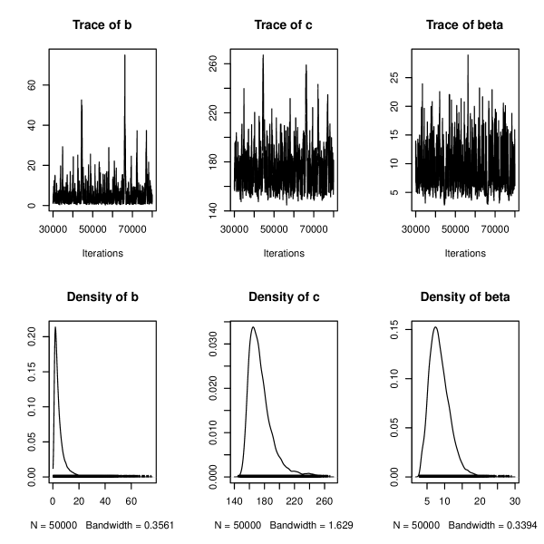
Figure 4: Trace plots of simulated parameter values of the Kumaraswamy inverse Weibull distribution.

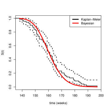
(a)

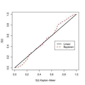
(b)

Figure 5: (a) Comparison among survivals generated by the method Bayesian and Kaplan-Meier described in the graph S(t) versus time. (b) Comparison among survivals generated by the method Bayesian described in the graph S(t) versus Kaplan- Meier.

6 Conclusions

We worked a three parameter lifetime distribution called the Kumaraswamy Inverse Weibull (Kum-IW) distribution which extends Inverse Weibull distribution proposed and widely used in the lifetime literature. The model is much more flexible than the inverse Weibull. The Kum-IW distribution could have increasing, decreasing and unimodal hazard rates. We provide a mathematical overview of this distribution including the densities of the order statistics, Rényi entropy, Shannon entropy, Bonferroni and Lorenz curves and Mean deviations. Also, we derive an explicit algebraic formula for the $r$-th moment, expressions for the order statistics, and the maximum likelihood estimation for the censored data. The performance of the model was analized using real data sets where the Kum-IW distribution performed verywell and the estimation was given by Bayes method.

References

• Carrasco etΒ al., (2008) Carrasco, J.Β F., Ortega, E. M.Β M., and Cordeiro, G.Β M. (2008). A generalized modified Weibull distribution for lifetime modeling. Computational Statistics & Data Analysis, 53(2):450 – 462.
• Cordeiro and deΒ Castro, (2011) Cordeiro, G.Β M. and deΒ Castro, M. (2011). A new family of generalized distributions. Journal of Statistical Computation and Simulation, 81(7):883–898.
• GusmΓ£o etΒ al., (2011) GusmΓ£o, F. R.Β S., Ortega, E. M.Β M., and Cordeiro, G.Β M. (2011). The generalized inverse Weibull distribution. Statistical Papers, 52:591–619.
• GusmΓ£o etΒ al., (2012) GusmΓ£o, F. R.Β S., Ortega, E. M.Β M., and Cordeiro, G.Β M. (2012). Reply to the Letter to the Editor of M. C. Jones. Statistical Papers, 53:252–254.
• Gupta etΒ al., (1999) Gupta, R.D., Kundu, D. (1999). Generalized exponential distribution. Australian and New Zeland Journal of Statistics. 41(2):173–188.
• Mudholkar etΒ al., (1995) Mudholkar, G.Β S., Srivastava, D.Β K., and Freimer, M. (1995). The exponentiated Weibull family: A reanalysis of the bus-motor-failure data. Technometrics, 37(4):436–445.
• Kass etΒ al., (1996) Kass, R.E., Wasserman, L. (1996). The Selection of Priori Distributions by Formal Rules. Journal of teh American Statistics Association, 91: 1343–1370.
• Kumaraswamy, (1980) Kumaraswamy, P. (1980). A generalized probability density function for double-bounded random processes. Journal of Hydrology, 46(1?2):79 – 88.
• Pescim etΒ al., (2010) Pescim, R.Β R., DemΓ©trio, C. G.Β B., Cordeiro, G.Β M., Ortega, E. M.Β M., and Urbano, M.Β R. (2010). The beta generalized half-normal distribution. Computational Statistics & Data Analysis, 54(4):945–957.
• Pollard, (1986) Pollard, W. E. (1986). Bayesian statistics for evaluation research An Introduction. Sage Publications New Delhi, 241p.
• Spiegelhalter etΒ al., (2007) Spiegelhalter, D., Thomas, A., Best, N., Lunn, D. (2007). Winbugs user manual, Version 1.4.3.
• R Core Team, (2012) R Core Team (2012). R: A Language and Environment for Statistical Computing. R Foundation for Statistical Computing, Vienna, Austria. ISBN: 3-900051-07-0.
• Xie and Lai, (1996) Xie, M. and Lai, C.Β D. (1996). Reliability analysis using an additive Weibull model with bathtub-shaped failure rate function. Reliability Engineering & System Safety, 52(1):87 – 93.