Scaling violation and relativistic effective mass from quasielastic electron scattering: implications for neutrino reactions

Abstract

The experimental data from quasielastic electron scattering from ¹²C are reanalyzed in terms of a new scaling variable suggested by the interacting relativistic Fermi gas with scalar and vector interactions, which is known to generate a relativistic effective mass for the interacting nucleons. By choosing a mean value of this relativistic effective mass $m_{N}^{*}=0.8m_{N}$, we observe that most of the data fall inside a region around the inverse parabola-shaped universal scaling function of the relativistic Fermi gas. This suggests a method to select the subset of data that highlight the quasielastic region, about two thirds of the total 2,500 data. Regardless of the momentum and energy transfer, this method automatically excludes the data that are not dominated by the quasielastic process. The resulting band of data reflects deviations from the perfect universality, and can be used to characterize experimentally the quasielastic peak, despite the manifest scaling violation. Moreover we show that the spread of the data around the scaling function can be interpreted as genuine fluctuations of the effective mass $M^{*}\equiv m^{*}_{N}/m_{N}\sim 0.8\pm 0.1$. Applying the same procedure we transport the scaling quasielastic band into a theoretical prediction band for neutrino scattering cross section that is compatible with the recent measurements and slightly more accurate.

Quasielastic electron scattering from nuclei has experienced a revival out of the practical need to gauge the validity of the current models as applied to neutrino scattering and oscillation experiments Nomad09 ; Agu10 ; Agu13 ; Fio13 ; Abe13 (for recent reviews see refs. Gal11 ; For12 ; Mor12 ; Alv14 ). The conventional approach pursues a detailed microscopic relativistic description of the inelastic processes and then requires all the relevant mechanisms for the particular $Q^{2}$ kinematics. At present there is no compelling model able to describe the world $(e,e^{\prime})$ experiments. In the case of ¹²C, taken as example here, the more than 2,500 data available spread over a huge $(q,\omega)$ kinematical region, reaching well inside the relativistic regime. A crucial issue is to find which electron data encode the maximum information to be applied to neutrino scattering minimizing the systematic and theoretical uncertainties in the relevant channel (quasielastic, pion emission, …). The scaling approach provides an appealing and unified framework to encompass coherently the large diversity of data stemming from different experiments and kinematics. In particular the super-scaling approach (SuSA) has been implemented along these lines to predict neutrino scattering cross sections from a longitudinal scaling function $f_{L}(\psi^{\prime})$ fitted to electron data Ama04 . Moreover, the recent upgrade of the SuSA-v2 Gon14 includes nuclear effects which are theoretically-inspired in a particular realization of the relativistic mean field (RMF) theory, by an additional transverse scaling function $f_{T}(\psi^{\prime})$ which is different from $f_{L}(\psi^{\prime})$.

A peculiar feature of the RMF is that it is the only approach which reproduces the experimental scaling function $f_{L}(\psi^{\prime})$ for all the values of $q$ after an ad-hoc $q$-dependent shift in energy is applied Ama05 . The theoretical origin of this phenomenological shift has not been well understood Gon14 . This model incorporates a dynamical enhancement of lower Dirac components, which is transmitted to the transverse response, $R_{T}$, improving the agreement with experimental data. However, gauge invariance is violated and hence $R_{T}$ still presents ambiguities Cab07 . Another difficulty of the RMF and other finite nuclei models is that they break translational invariance (attempts to restore it in a relativistic system were explored in refs. Alb05 ; Alb07 ).

The goal of this paper is to exploit the scaling idea from a novel point of view connecting the RMF with the universal scaling function of the relativistic Fermi gas (RFG)

$$f(\psi^{*})=\frac{3}{4}(1-\psi^{*}{}^{2})\theta(1-\psi^{*}{}^{2})$$ (1)

Rather than constructing a yet undetermined scaling function we aim to propose a new scaling variable $\psi^{*}$ mapping the data into a region around the above function. Inspired by the fact that the mean field theory provides a consistent and reasonable description of the nuclear response in the quasielastic region (already observed by Rosenfelder 35 years ago Ros80 ) for a range of kinematics, we propose to start from the interacting RFG Ser86 including a suitable vector and scalar potentials which are inferred from the data into an effective mass $m^{*}_{N}$ that gets reduced in the nuclear medium. The effective mass encodes relativistic dynamical effects relevant in this kinematical region, alternative to other approaches like the one based on the spectral function Ben08 ; Ank15 . In fact, one of the motivations of our approach, called here $M^{*}$-scaling (or M*S), was to provide a framework enjoying the good features of the RMF without incurring into the above mentioned difficulties, unvealing the $m^{*}_{N}$ origin of the dynamical enhancement of both the lower components and the transverse response function. The shift of $f_{L}(\psi^{\prime})$ is trivially obtained as a consequence of the $m^{*}$ dependence of the quasielastic peak position.

Of course, there have been numerous attempts to determine the effective mass Weh93 ; Mariano05 , but this depends on details of the dynamics. Thus, by proceeding directly from the data we avoid specifying the mean field explicitly. On the other hand a phenomenological determination of $m_{N}^{*}$ suffers from the uncertainties on the bulk of the data which should most significantly contribute. Therefore, we will from the beginning accept that this effective mass is determined up to a sensible uncertainty, defined precisely by a suitable selection of the large database, to be explained below in detail. One of the main advantages of this rather simple approach, is not only its ease of implementation, but also that we are free from the traditional objections regarding gauge invariance or PCAC violations. We expect in this way to account for the most relevant uncertainties regarding the predictive power of the model.

We follow closely the notation introduced in Ref. Alb88 . The quasielastic electroweak cross section is proportional to the hadronic tensor or response function for single-nucleon excitations transferring momentum ${\bf q}$ and energy $\omega$, which in the Fermi gas reads

$$W^{\mu\nu}(q,\omega) = \frac{V}{(2\pi)^{3}}\int d^{3}p\delta(E^{\prime}-E-\omega)\frac{(m_{N}^{*})^{2}}{EE^{\prime}}$$ (2)

$$\times 2w^{\mu\nu}_{s.n.}({\bf p}^{\prime},{\bf p})\theta(k_{F}-p)\theta(p^{\prime}-k_{F})$$

where $E=\sqrt{{\bf p}^{2}+m_{N}^{*}{}^{2}}$ is the initial nucleon energy in the mean field. The final momentum of the nucleon is ${\bf p}^{\prime}={\bf p}+{\bf q}$ and its energy is $E^{\prime}=\sqrt{{\bf p}^{\prime}{}^{2}+m_{N}^{*}{}^{2}}$. Note that initial and final nucleons have the same effective mass $m_{N}^{*}$. The volume $V=3\pi^{2}N/k_{F}^{3}$ of the system related to the Fermi momentum $k_{F}$ and proportional to the number $N$ of protons and/or neutrons participating in the process. Finally the electroweak interaction mechanism is implicit in the single-nucleon tensor

$$w^{\mu\nu}_{s.n.}({\bf p}^{\prime},{\bf p})=\frac{1}{2}\sum_{ss^{\prime}}J^{\mu*}({\bf p}^{\prime},{\bf p})J^{\nu}({\bf p}^{\prime},{\bf p})$$ (3)

where $J^{\mu*}$ is the electroweak current matrix element between free positive energy Dirac spinors, with mass $m_{N}^{*}$ and normalized to $\overline{u}u=1$. In the case of electron scattering we are involved with the electromagnetic current matrix element

$$J^{\mu}_{s^{\prime}s}({\bf p}^{\prime},{\bf p})=\overline{u}_{s^{\prime}}({\bf p}^{\prime})\left[F_{1}(Q^{2})\gamma^{\mu}+F_{2}(Q^{2})i\sigma^{\mu\nu}\frac{Q_{\nu}}{2m_{N}}\right]u_{s}({\bf p})$$ (4)

where $F_{1}$ and $F_{2}$ are, respectively, the Dirac and Pauli electromagnetic form factors of proton or neutron.

In the case of $(e,e^{\prime})$ the quasielastic cross section is written in Rosenbluth form

$$\frac{d\sigma}{d\Omega^{\prime}d\epsilon^{\prime}}=\sigma_{\rm Mott}\left(v_{L}R_{L}+v_{T}R_{T}\right)$$ (5)

where $\sigma_{\rm Mott}$ is the Mott cross section, $v_{L}=Q^{4}/q^{4}$ and $v_{T}=\tan^{2}(\theta/2)-Q^{2}/2q^{2}$, with $\theta$ the scattering angle. The nuclear longitudinal and transverse response functions are the following components of the hadronic tensor in a coordinate sustem with the $z$-axis in the ${\bf q}$ direction (longitudinal)

$$R_{L}(q,\omega) = W^{00}$$ (6)

$$R_{T}(q,\omega) = W^{11}+W^{22}$$ (7)

In the RFG the nuclear response functions can be written in the factorized form for $K=L,T$

$$R_{K} = G_{K}f(\psi^{*}),$$ (8)

$$G_{K} = \Lambda(ZU^{p}_{K}+NU^{n}_{K})$$ (9)

Where $f(\psi^{*})$ is given in Eq. (1) and $\psi^{*}$ is defined below. Moreover

$$\Lambda=\frac{\xi_{F}}{m^{*}_{N}\eta_{F}^{3}\kappa}$$ (10)

and the single nucleon response functions are

$$U_{L} = \frac{\kappa^{2}}{\tau}\left[(G^{*}_{E})^{2}+\frac{(G_{E}^{*})^{2}+\tau(G_{M}^{*})^{2}}{1+\tau}\Delta\right]$$ (11)

$$U_{T} = 2\tau(G_{M}^{*})^{2}+\frac{(G_{E}^{*})^{2}+\tau(G_{M}^{*})^{2}}{1+\tau}\Delta$$ (12)

where the quantity $\Delta$ has been introduced

$$\Delta=\frac{\tau}{\kappa^{2}}\xi_{F}(1-\psi^{*}{}^{2})\left[\kappa\sqrt{1+\frac{1}{\tau}}+\frac{\xi_{F}}{3}(1-\psi^{*}{}^{2})\right].$$ (13)

Dimensionless variables have been introduced measuring the energy and momentum in units of $m_{N}^{*}$, namely $\lambda=\omega/2m_{N}^{*}$, $\kappa=q/2m_{N}^{*}$, $\tau=\kappa^{2}-\lambda^{2}$, $\eta_{F}=k_{F}/m_{N}^{*}$, and $\xi_{F}=\sqrt{1+\eta_{F}^{2}}-1$. Note that usually Alb88 these variables are defined with respect to the nucleon mass $m_{N}$ instead of the $m_{N}^{*}$. The same can be said with respect to the electric and magnetic form factors, that are modified in the medium due to the effective mass according to

$$G_{E}^{*} = F_{1}-\tau\frac{m^{*}_{N}}{m_{N}}F_{2}$$ (14)

$$G_{M}^{*} = F_{1}+\frac{m_{N}^{*}}{m_{N}}F_{2}.$$ (15)

One should still stress that $F_{1}$ and $F_{2}$ can depend on $M^{*}$ Sai04 . We stick here to the phenomenologically succsessfull CC2 prescription that reproduces the experimental superscaling function Cab07 . Using the CC1 operator obtained through the Gordon reduction produces the same effects as in the RMF of ref. Cab07 . The same modification of form factors in the medium was explored in ref. Bar98 . For the free form factors we use the Galster parametrization.

To define the scaling variable, $\psi^{*}$, we first introduce the minimum energy allowed for a nucleon inside the nucleus to absorb the virtual photon (in units of $m_{N}^{*}$)

$$\epsilon_{0}={\rm Max}\left\{\kappa\sqrt{1+\frac{1}{\tau}}-\lambda,\epsilon_{F}-2\lambda\right\}$$ (16)

where $\epsilon_{F}=\sqrt{1+\eta_{F}^{2}}$ is the Fermi energy in units of $m_{N}^{*}$. The scaling variable is defined by

$$\psi^{*}=\sqrt{\frac{\epsilon_{0}-1}{\epsilon_{F}-1}}{\rm sgn}(\lambda-\tau)$$ (17)

Note that $\psi^{*}<0$ for $\lambda<\tau$ (the left side of the quasielastic peak). The meaning of $\psi^{*}{}^{2}$ is the following: it is the minimum kinetic energy of the initial nucleon divided by the kinetic Fermi energy.

Starting with the experimental $(e,e^{\prime})$ cross section we compute the experimental scaling function $f_{\rm exp}$

$$f_{\rm exp}=\frac{\left(\frac{d\sigma}{d\Omega^{\prime}d\epsilon^{\prime}}\right)_{\rm exp}}{\sigma_{\rm Mott}\left(v_{L}G_{L}+v_{T}G_{T}\right)}$$ (18)

which would correspond to the function $f(\psi^{*})$ in the relativistic Fermi gas model.

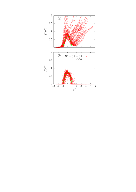
Figure 1: Top panel (a): $M*$ scaling analysis of the experimental data of ¹²C as a function of the scaling variable $\psi^{*}$ for $M^{*}=m^{*}_{N}/m_{N}=0.8$ compared to the RFG parabola. Bottom panel (b): RFG Monte Carlo simulation of QE data with a Gaussian distribution of relativistic effective mass quotient around $M^{*}=0.8\pm 0.1$. The Fermi momentum is fixed to $k_{F}=225$ MeV/c.

We summarize the results of our M*S analysis in figure 1a. We plot the experimental scaling function for the bulk of ¹²C data archive ; archive2 as a function of the scaling variable $\psi^{*}$. We take

$$M^{*}=\frac{m_{N}^{*}}{m_{N}}=0.8.$$ (19)

We see that a large fraction of the data collapse into a data cloud surrounding the RFG scaling function, given by Eq (1). Other choices of $m^{*}_{N}$ are possible but the clustering substantially detunes from the RFG. So we interpret this pattern as the kinematic regions highlighting the effective Fermi gas behavior of data. This collapse of data resolves two issues simultaneously: On the theoretical side it provides an operational definition of the relativistic effective mass, whereas on the experimental side provides an operational definition of the quasielastic peak behavior.

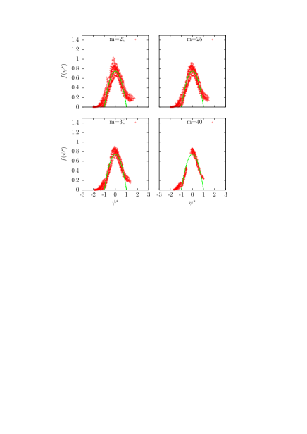
Figure 2: Experimental data selection in terms of the scaling variable $\psi^{*}$, obtained with different choices of the number $m$ of points inside a circle with radius $r=0.1$.

The observed scaling is not perfect in the sense that the blur of data presents a finite width, but the width is roughly homogeneous as seen in Fig. 2. There we select the data that are clustered on a coarse grain scale according to a method inspired by the visual and conventional Gaussian low-pass filtering (Gaussian blur) Gauss . Due to the discrete, heterogeneous and finite nature of the data in our case we use instead a constant weighting function. This function measures the density of points clustered above a given threshold $m$, inside a circle of radius $r$ centered at the experimental point, plus minus the experimental error. In the figure we show four situations corresponding to $r=0.1$, and for illustration the result of applying our low pass filtering method to four values of $m=20,25,30$ and 40. The parameter $m$ measures the minimum number of experimental points surrounding each data in the cloud. Note that we discard the surrounding points that don’t verify the above condition. As we can see the shape defined by the data cloud, seen as a shaded band in the scale of the figure, presents a stable pattern around the relativistic Fermi gas when the threshold value increases, even if the number of surviving points decreases. This stability around the Fermi gas result is triggered by the chosen value of $M^{*}$. Note that the number of data involved in these plots is around 1,500, but the scaling violation (defined as the width of the shaded band) is manifest.

This pattern in the M*S plot, that emerges as a realization of an universal quasielastic peak, is a global property of the set of data and suggests an alternative interpretation in terms of fluctuations of $M^{*}$. One could propose a statistical model where each point in the cloud samples a quasielastic event with a slightly different effective mass around the mean value 0.8. This fluctuation does not simulate the nuclear effects beyond the impulse approximation (finite size effects, short-range NN-correlations, long-range RPA, meson-exchange currents, $\Delta$ excitation, pion emission, two-particle emission, final state interaction). However the fluctuations are of the same order of magnitude as these effects. Actually they are small enough to retain the points in the neighborhood of the quasielastic region, which could be treated perturbatively in a microscopic framework beyond the RFG. The largest deviations of the quasielastic cloud from the perfect parabola occur only around its edges, where the Fermi gas is zero and hence the resulting signal cannot be accounted for by a change of $m_{N}^{*}$.

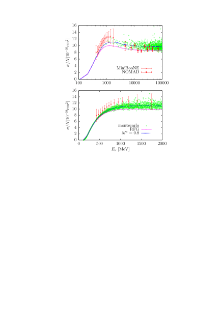
Figure 3: Total QE neutrino cross section off ¹²C per neutron as a function of the neutrino energy for different relativistic effective masses generated in a Monte Carlo simulation. The experimental data points are from NOMAD Nomad09 and MiniBooNE Agu10 . We take the axial dipole mass $M_{A}=1$ GeV.

To justify the above assumption, we carried out a calculation using a family of RFGs with slightly different $m^{*}_{N}$, to generate a random point for each single experimental datum at the very same kinematics. Thus we take a random $M^{*}$ around the optimal mean value 0.8 in a Monte Carlo sampling. The results of this simulation are shown in Fig.1-b. To generate the pseudo data we use a Gaussian distribution with a width value $\sigma=0.1$, representing the fluctuation of $M^{*}=0.8\pm 0.1$, that nicely resembles the fluctuations seen in the cloud of the experimental data. This procedure automatically selects those pseudo data attributable to genuine quasielastic interpretation (based on the Fermi gas definition) and makes zero those kinematics that are forbidden.

Our main observation is that by choosing the optimum relativistic effective mass, a RFG-like scaling of the data can be obtained in the quasielastic region, covering more than 1500 data. This implies a trade off between the experimental uncertainty to what extent a datum is close to quasielastic and the importance of the physical effects beyond the impulse approximation that contribute to the quasielastic mechanism. With this procedure a way to estimate what information is contained in the data about the quasielastic peak emerges.

From our analysis a phenomenological scaling function could be also obtained exactly in the same way as in the superscaling analysis. We have not tried to parameterize this function, that could be done from the data of fig. 2. The resulting scaling function is asymmetrical and very similar to the longitudinal superscaling function, but with a different normalization, including the tail. Therefore the tail of the scaling function is a property of the quasielastic interaction.

The information extracted here about the quasielastic $(e,e^{\prime})$ cross section of ¹²C can be straightforwardly used to make readily predictions for other reactions like CC neutrino scattering from the same nucleus. In figure 3 we show the calculations of the $(\nu_{\mu},\mu^{-})$ cross section as a function of incident neutrino energy. There we show the effective RFG results with $m_{N}^{*}=0.8m_{N}$. The cloud of points correspond to incorporating the same fluctuations $\pm 0.1$ of $M^{*}$ as in the Monte Carlo simulation depicted in Fig. 1-b. By comparison we also show the results of the conventional RFG. The effective mass produces an enhancement of the lower Dirac components, and hence also of both the vector and axial transverse responses, and of the theoretical cross section, which thanks to the fluctuations becomes compatible with the data for all the kinematics. In our case the fluctuations of the theoretical band are about 10%, as naively expected from the input uncertainty of the effective mass. We note that the sampling in the lower panel of figure 3 uses a smaller binning of 1 MeV as opposed to the upper panel where 100 MeV was used instead. The clustering of these equidistant binnings arises naturally from the log scale.

For high $Q$ the vector form factors deviate from the conventional dipole behaviour Bod08 , which could affect, in principle, any model’s predictions. However this would only be appreciable in the differential cross section; the integrated $\sigma$, even for NOMAD kinematics, is only sensitive to the kinematical regions where the product of form factors and phase space is large. We have numerically checked that the contribution from $Q^{2}$ above 1-2 (GeV/c)² is negligible, because of the rapid fall of the nucleon form factors. As a matter of fact one can ignore the electric neutron form factor completely after integration.

Note that the set of data of unfolded energy dependent CCQE cross section model suffer from uncertainties driven by the model dependence of the neutrino energy reconstruction. The comparison of fig. 3 is merely indicative for illustration purposes of the kind of predictions that the present approach can provide for proper flux-averaged doubly differential cross sections. These comparison will be presented in a forthcoming publication.

At present there is no model able to reproduce the 2,500 data points from ${}^{12}C(e,e^{\prime})$ experiments. Due to the impossibility to fit the quasielastic peak or other regions with the experimental accuracy, in the present approach, we have shown that instead of making an extremely detailed analysis of the particular reaction, which maybe well beyond the present validation possibilities, it is possible to isolate those data contributing to the simplest possible physics we are interested in, and use that information to make predictions with the maximum allowed precision, since one cannot distinguish the theoretical noise from the experimental signal.

References

- (1) V Lyubushkin et al. (NOMAD Collaboration), Eur. Phys. J. C 63 (2009), 355.
- (2) A. Aguilar-Arevalo et al. (MiniBooNE Collaboration), Phys. Rev. D 81, 092005 (2010).
- (3) A. Aguilar-Arevalo et al. (MiniBooNE Collaboration), Phys. Rev. D 88, 032001 (2013).
- (4) G.A. Fiorentini et al. (MINERvA Collaboration) Phys. Rev. Lett. 111, 022502 (2013).
- (5) K. Abe et al., (T2K Collaboration), Phys. Rev. D 87, 092003 (2013).
- (6) H. Gallagher, G. Garvey, G.P. Zeller, Annu. Rev. Nucl. Part. Sci. 61, 355 (2011).
- (7) J.A. Formaggio, G.P. Zeller, Rev. Mod. Phys. 84, 1307 (2012).
- (8) J.G. Morfin, J. Nieves, J.T. Sobczyk, Adv. High Energy Phys. 2012, 934597 (2012).
- (9) L. Alvarez-Ruso, Y. Hayato, and J. Nieves, New Jou. Phys. 16 (2014) 075015.
- (10) J. E. Amaro, M. B. Barbaro, J. A. Caballero, T. W. Donnelly, A. Molinari, I. Sick, Phys. Rev. C 71, 015501 (2005).
- (11) R. Gonzalez-Jimenez, G.D. Megias, M.B. Barbaro, J.A. Caballero, and T.W. Donnelly, Phys. Rev. C 90, 035501 (2014).
- (12) J. E. Amaro, M. B. Barbaro, J. A. Caballero, T. W. Donnelly, C. Maieron, Phys. Rev. C 71, 065501 (2005).
- (13) J.A. Caballero, J. E. Amaro, M. B. Barbaro, T. W. Donnelly, J.M. Udias, Phys. Lett. B 653, 366 (2007).
- (14) P. Alberto, S.S. Avancini, and M. Fiolhais, Int. Jou. Mod. Phys. E 14 (2005) 1171.
- (15) P. Alberto, S.S. Avancini, M. Fiolhais, and J.R. Marinelli Phys. Rev. C 75 (2007) 054324.
- (16) R. Rosenfelder, Ann. Phys. (N.Y:) 128, 188 (1980)
- (17) B.D. Serot, and J.D. Walecka, Adv. Nucl. Phys. 16 (1986) 1.
- (18) O. Benhar, D. Day, and I. Sick, Rev Mod Phys. 80 (2008) 189
- (19) A. M. Ankowski, O. Benhar, M. Sakuda, Phys. Rev. D 91, 033005 (2015).
- (20) K. Wehrberger, Phys. Rep. 225 (1993) 273.
- (21) A. Mariano, and C. Barbero, J. Phys. G 31 (2005) 119.
- (22) W.M. Alberico, A. Molinari, T.W. Donnelly, E. L. Kronenberg, and J.W. Van Orden, Phys Rev. C 38 (1988) 1801.
- (23) Saito et al., Prog.Part.Nucl.Phys. 58 (2007) 1-167; Tsushima et al., Phys.Rev. C70 (2004) 038501.
- (24) M.B. Barbaro, R. cenni, A. De pace, T.W. Donnelly, A. Molinari, Nucl. Phys. A 643 (1998) 137.
- (25) A. Bodek, S. Avvakumov, R. Bradford, H. S. Budd Eur. Phys. J. C53 (2008) 349.
- (26) Benhar, Day and Sick, arXiv:nucl-ex/0603032.
- (27) http://faculty.virginia.edu/qes-archive/
- (28) Lessons from the masters: current concepts in astronomical image processing. Robert Gendler, Editor. Springer, New York, 2013.