The age-metallicity relationship in the Small Magellanic Cloud periphery

Abstract

We present results from Washington $CT_{1}$ photometry for eleven star fields located in the western outskirts of the Small Magellanic Cloud (SMC), which cover angular distances to its centre from 2 up to 13 degrees ($\approx$ 2.2 $-$ 13.8 kpc). The colour-magnitude diagrams, cleaned from the unavoidable Milky Way (MW) and background galaxy signatures, reveal that the most distant dominant main sequence (MS) stellar populations from the SMC centre are located at an angular distance of $\sim$ 5.7 deg (6.1 kpc); no sign of farther clear SMC MS is visible other than the residuals from the MW/background field contamination. The derived ages and metallicities for the dominant stellar populations of the western SMC periphery show a constant metallicity level ([Fe/H] = -1.0 dex) and an approximately constant age value ($\approx$ 7$-$8 Gyr). Their age-metallicity relationship (AMR) do not clearly differ from the most comprehensive AMRs derived for almost the entire SMC main body. Finally, the range of ages of the dominant stellar populations in the western SMC periphery confirms that the major stellar mass formation activity at the very early galaxy epoch peaked $\sim$ 7-8 Gyr ago.

1 Introduction

Our knowledge about the age-metallicity relationship (AMR) of the Small Magellanic Cloud (SMC) has improved since recent -some of them still ongoing- systematic photometric studies have been carried out (e.g. Subramanian & Subramaniam, 2012; Cignoni et al., 2013; Weisz et al., 2013; Rubele et al., 2015). From an overall consensus about the formation and chemical evolution of this galaxy, some features can be highlighted: i) an initial period of low star formation rate (SFR); ii) an older enhanced star formation process that peaked at $\sim$ 8 Gyr ago; iii) another periods of intense SFR at $\sim$ 1.5$-$2.5 and 5$-$6 Gyr, consistent with suggestions of close encounter with the Large Magellanic Cloud (LMC) and/or the Milky Way (MW); iv) field stars do not possess gradients in age and metallicity; v) an AMR with a clear steady enrichment of the galactic metal content with time (older stellar populations are more metal-poor), with some variations, among others.

These main results picture the presently known assembled scenario for the formation and chemical evolution of the SMC main body; the farthest studied star field is located at $\sim$ 6.5 kpc from its centre (Noël & Gallart, 2007; Carrera et al., 2008; Noël et al., 2009). However, the SMC periphery, particularly the portion towards the opposite direction to the LMC, could harbour primordial stellar populations not yet comprehensively dealt with. Nidever et al. (2011) carried out a photometric survey of the SMC periphery, from which they extracted a modelled galactic geometry using giant star counts; no detailed study about the spatial behaviour of star field ages and metallicities were performed.

Piatti (2012a, hereafter P12) accomplished an AMR study of the SMC stellar populations from Washington $CT_{1}$ photometry of 12 star fields (36$\times$36 armnin² each) getting a compromise between covering a relatively large area and reaching the oldest main sequence turnoffs (MSTOs). He found that the field stars do not possess gradients in age and metallicity, and that stellar populations formed since $\sim$ 2 Gyr ago are more metal-rich than [Fe/H] $\sim$ -0.8 dex and are confined to the innermost regions (semi-major axis $\leq$ 1 deg), along with relatively more metal-poor ([Fe/H] $\sim$ -1.0 $-$ -1.5 dex) and older (age $\sim$ 3$-$8 Gyr) field stars. He also compared the field star AMR to that of the star cluster population with ages and metallicities in the same star field scale, and found that clusters and star fields share similar chemical evolution histories. Nevertheless, the outermost star field studied by P12 is located $\sim$ 4.9 kpc, so that the AMR in the SMC periphery has remained mostly unstudied.

In this paper we continue the work of P12 by studying other 11 SMC fields located in the western outskirts of the SMC. As a matter of consistency, we also analyse a Washington $CT_{1}$ data set using the same techniques. We aim at characterizing the dominant stellar populations distributed in that region and providing for the first time with a representative AMR. For these purposes, we structured the paper as follows: Section 2 deals with the description of the photometric data sets, the reduction processes and the various calibrations involved, including error and completeness analyses. The observed colour-magnitude diagram (CMD) features as well as the cleaning procedures for decontaminating them from the MW/background galaxy signatures are described in Section 3. In Section 4 we estimate the ages and metallicities of the dominant stellar populations in each SMC field, and discuss their AMR to the light of the most comprehensively known SMC AMRs. Concluding remarks are given in Section 5.

2 Data handling

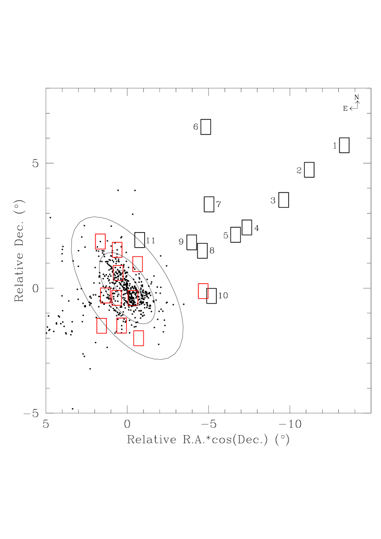
Figure 1: Spatial distribution of the presently studied SMC star fields (thick black boxes) and of those in P12 (thick red boxes). Star clusters catalogued by Bica et al. (2008) are also drawn (dots) for comparison purposes. Ellipses with semi-major axes of 1, 2 and 4 deg are overplotted.

In our previous series of studies of SMC clusters and star fields (see, e.g. Piatti, 2011c, P12) we used the Washington $CT_{1}$ photometric system (Canterna, 1976) from which ages and metallicities for stellar populations older than $\sim$ 1 Gyr can be estimated (Piatti & Perren, 2015, and references therein). For these reasons, and in order to keep consistency with our previous studies, we performed a search within the National Optical Astronomy Observatory (NOAO) Science Data Management (SDM) Archives seeking for Washington photometric data towards the SMC periphery. As a result, we found images obtained at the Cerro-Tololo Inter-American Observatory (CTIO) 4m Blanco telescope with the Mosaic II camera (36$\times$36 arcmin² field with a 8K$\times$8K CCD detector array, scale 0.274 arcsec/pixel) covering 11 fields in the SMC outskirts for a total area of $\sim$ 4.0 square degrees (programme CTIO 2006B-0013, PI: Saha). The log of the observations is presented in Table 1, where the main astrometric, photometric and observational information is summarized. Note that the data set includes the filter $R$ which is a more efficient substitute of the $T_{1}$ filter (Geisler, 1996), but our final standard magnitude is the Washington $T_{1}$ mag. Fig. 1 depicts the spatial distribution of the SMC fields, where we included those in P12 for comparison purposes. The maximum angular distance probed from the centre of the SMC is $\sim$ 13.0 deg.

The Washington $CT_{1}$ photometric data set used in this work were obtained from a comprehensive process that involved the reduction of the raw images, the determination of the instrumental photometric magnitudes, and the standardization of the photometry. We have already described in detail such steps not only in the works cited above, but also in Piatti (2011b, c, a, 2012b); Piatti & Bica (2012); Piatti, Geisler & Mateluna (2012); Maia, Piatti & Santos (2014). For this reason, we summarize here some specific issues in order to provide the reader with an overview of the photometry quality. The data reduction followed the procedures documented by the NOAO Deep Wide Field Survey team (Jannuzi, Claver & Valdes, 2003) and utilized the mscred package in IRAF. We performed overscan, trimming and cross-talk corrections, bias subtraction, flattened all data images, etc., once the calibration frames (zeros, sky- and dome- flats, etc) were properly combined. For each image we obtained an updated world coordinate system (WCS) database with a rms error in right ascension and declination smaller than 0.4 arcsec, by using $\sim$ 500 stars catalogued by the USNO.

We also retrieved MOSAIC II and CTIO 0.9m CFCCD images of the standard fields SA 92 and SA 98 observed as part of the same programme. The reduction of the MOSAIC II data set was performed following the steps as for the SMC fields. These standard fields contain between 8 and 14 standard stars each (Geisler, 1996) and series of eight observations were carried out by dithering the images, so that most of the standard stars were distributed on each of the MOSAIC II’s eight chips. This observing procedure was repeated for different airmasses. The images from the CTIO 0.9m telescope were taken with the Tektronix 2K#3 CCD, using quad-amp readout. The scale on the chip is 0.4 arcsec/pixel yielding an area covered by a frame of 13.5$\times$13.5 arcmin². The integrated IRAF-Arcon 3.3 interface for direct imaging was employed as the data acquisition system. The data were processed using the QUADPROC package in IRAF. After applying the overscan-bias subtraction for the four amplifiers independently, we carried out flat-field corrections using a combined sky-flat frame, which was previously checked for a non-uniform illumination pattern with the averaged dome-flat frame.

We derived nearly 80 independent magnitude measures of standard stars per filter for each night using the apphot task within IRAF, in order to secure the transformation from the instrumental to the Washington $CT_{1}$ standard system. The relationships between instrumental and standard magnitudes were obtained by fitting the equations:

$$c=a_{1}+T_{1}+(C-T_{1})+a_{2}\times X_{C}+a_{3}\times(C-T_{1}),$$ (1)

$$r=b_{1}+T_{1}+b_{2}\times X_{R}+b_{3}\times(C-T_{1}),$$ (2)

where $a_{i}$ and $b_{i}$ ($i$ = 1, 2, and 3) are the fitted coefficients, and $X$ represents the effective airmass. Capital and lowercase letters represent standard and instrumental magnitudes, respectively. We solved the transformation equations with the fitparams task in IRAF for each night, and substituted the derived mean zero point and colour term ($a_{3}$ = -0.090, $b_{3}$ = -0.020) values for each observing run into the above equations and solved for the airmass coefficient for each night. Typical values of $a_{2}$ and $b_{2}$ were 0.305 and 0.095 mag/airmass, respectively. The nightly rms errors from the transformation to the standard system were 0.021 and 0.017 mag for $C$ and $T_{1}$, respectively, indicating the nights were of excellent photometric quality.

The stellar photometry was performed using the star-finding and point-spread-function (PSF) fitting routines in the daophot/allstar suite of programs (Stetson, Davis & Crabtree, 1990). We measured magnitudes on the single image created by joining all 8 chips together using the updated WCS. This allowed us to use a unique reference coordinate system for each SMC field. For each Mosaic image, a quadratically varying PSF was derived by fitting $\sim$ 1000 stars (nearly 110-130 stars per chip), once the neighbours were eliminated using a preliminary PSF derived from the brightest, least contaminated $\sim$ 250 stars (nearly 30-40 stars per chip). Both groups of PSF stars were interactively selected. We then used the allstar program to apply the resulting PSF to the identified stellar objects and to create a subtracted image which was used to find and measure magnitudes of additional fainter stars. This procedure was repeated three times for each frame. We computed aperture corrections from the comparison of PSF and aperture magnitudes by using the neighbour-subtracted PSF star sample. After deriving the photometry for all detected objects in the $C$ and $T_{1}$ filters, a cut was made on the basis of the parameters returned by DAOPHOT. Only objects with $\chi$ $<$2, photometric error less than 2$\sigma$ above the mean error at a given magnitude, and $|$SHARP$|$ $<$ 0.5 were kept in each filter, and then the remaining objects in the $C$ and $T_{1}$ lists matched with a tolerance of 1 pixel.

Finally, we standardized the resulting instrumental magnitudes and combined all the independent measurements using the stand-alone daomatch and daomaster programs. The final information for each field consists of a running number per star, its right ascension and declination coordinates, the averaged $T_{1}$ magnitude and $C-T_{1}$ colour, the standard errors $\sigma(T_{1})$ and $\sigma(C-T_{1})$ and the number of measurements in the $C$ and $T_{1}$ filters. Whenever a star does have only one measure of $C$ and $T_{1}$ mags, the errors provided by the daophot/allstar routines were listed. Table 2 gives this information for Field 1. Only a portion of this table is shown here for guidance regarding its form and content. The whole content of Table 2, as well as the final information for the remaining fields, is available in the online version of the journal.

As is well known, photometric errors, crowding effects and the detection limit of the images cause incompleteness and therefore results in the increasing loss of stars at fainter magnitudes. Commonly, artificial star tests on the deepest images are performed in order to derive the completeness level at different magnitudes. We used the stand-alone addstar program in the daophot package (Stetson, Davis & Crabtree, 1990) to add synthetic stars, generated at random with respect to position and magnitude, to each deepest image in order to derive its completeness level. We added a number of stars equivalent to $\sim$ 5$\%$ of the measured stars in order to avoid in the synthetic images significantly more crowding than in the original images. On the other hand, to avoid small number statistics in the artificial-star analysis, we created five different images for each original one. We used the option of entering the number of photons per ADU in order to properly add the Poisson noise to the star images.

We then repeated the same steps to obtain the photometry of the synthetic images as described above, i.e., performing three passes with the daophot/allstar routines. The star-finding efficiency were estimated by comparing the output and the input data for these stars using the daomatch and daomaster tasks. We illustrate in Fig. 2 the resultant completeness fractions in the $T_{1}$ versus $C-T_{1}$ CMD for the most pupolated field in our sample (Field 11). Fig. 2 shows that the 50$\%$ completeness level is located at $C$ $\sim$ 23.75 mag and $T_{1}$ $\sim$ 24.25 mag; for less crowded fields this completeness level reaches down to $\sim$ 0.75-1.00 mag fainter, depending on the crowding. Note that, according to the theoretical isochrones computed by Bressan et al. (2012) and considering the SMC distance modulus $(m-M)_{o}$ = 18.96 (de Grijs & Bono, 2015), a 13 Gyr old stellar population ([Fe/H] $\approx$ -1.3 dex) should have its MSTO at $T_{1}$ $\approx$ 22.5 mag. Therefore, our photometry reaches the 50$\%$ completeness level 2-3 mag below the oldest known SMC MSTOs (Carrera et al., 2008; Noël et al., 2009).

3 Global properties of the colour-magnitude diagrams

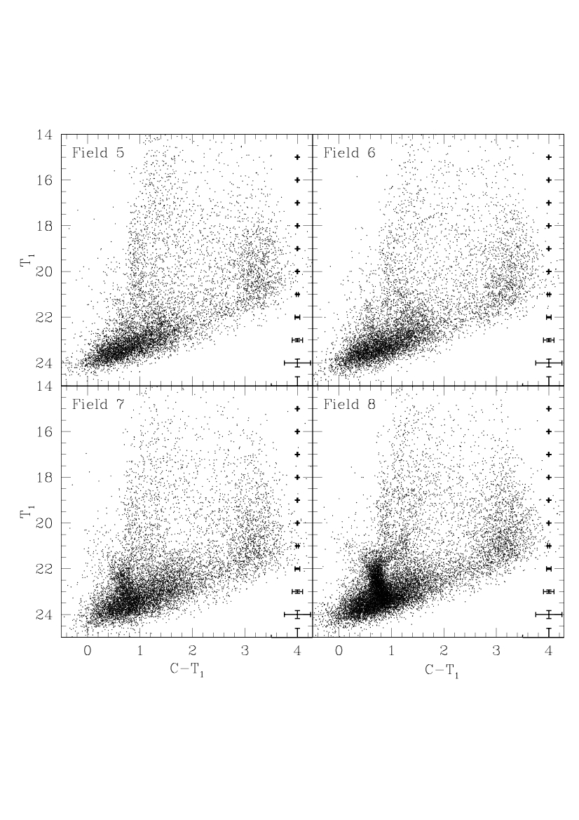
Figure 3: continued.

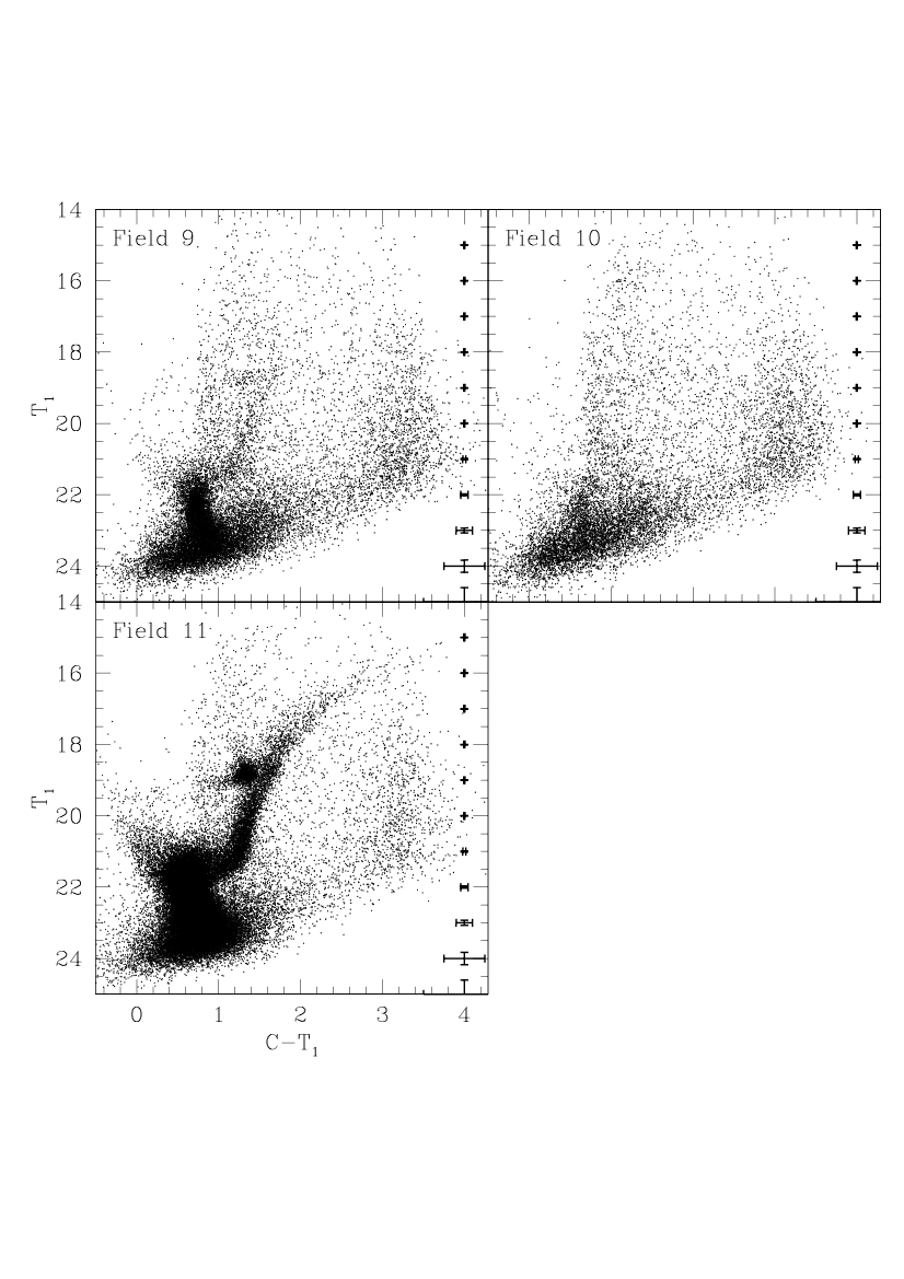
Figure 3: continued.

In Fig. 3 we plot the CMDs for all measured stars in each SMC field. We measured from $\sim$ 11 up to 76 thousand stars from the outermost to the innermost fields, with an average of $\sim$ 33 thousand stars, thus yielding a $CT_{1}$ photometric database of $\sim$ 175 thousand stars. The CMDs present a strong signature of the foreground/background fields which blurs the SMC outskirts main features. Nevertheless, it can be seen an old main sequence (MS) population in Field 7 ($C-T_{1}$ $\approx$ 0.8, $T_{1}$ $\sim$ 22-23), and increasing younger populations (brighter $T_{1}$ MSTOs) for inner SMC fields. Thus, the series of panels depicted in Fig. 3 show the age transition of the stellar populations in the outermost SMC regions. At the right margin of each panel we show the behaviour of the errors $\sigma$($T_{1}$) and $\sigma$($C-T_{1}$). As can be seen, it would seem that a relatively small dispersion accompanies the intrinsic features along almost $\sim$ 9 mags.

3.1 Cleaning the CMDs

In order to disentangle the MW/background signature in the peripheral SMC CMDs, we applied a procedure primarily developed by Piatti & Bica (2012, see, Fig. 12) to clean star cluster CMDs from field star contamination (see, e.g. Piatti, 2014; Piatti et al., 2014b, 2015). Comparisons of field and cluster CMDs have long been done by comparing the numbers of stars counted in boxes distributed in a similar manner throughout both CMDs. However, since some parts of the CMD are more densely populated than others, counting the numbers of stars within boxes of a fixed size is not universally efficient. For instance, to deal with stochastic effects at relatively bright magnitudes (e.g., fluctuations in the numbers of bright stars), larger boxes are required, while populous CMD regions can be characterized using smaller boxes. Thus, use of boxes of different sizes distributed in the same manner throughout both CMDs leads to a more meaningful comparison of the numbers of stars in different CMD regions.

For our purposes, we adopted Field 1 as the MW/background field CMD, which is located $\sim$ 3$-$4 deg farther than the SMC boundary delimited by Nidever et al. (2011). We also assumed that the MW/background field is uniform in terms of luminosity function, colour distribution and stellar density across the surveyed region (Balbinot et al., 2015). Note that the eleven SMC fields are projected over a relatively small MW area of $\sim$ 16$\times$7 deg². We checked this assumption for the MW by building a series of synthetic CMDs using the Besançon galactic model (Robin et al., 2003). Note that MW models can only include MW stars and not distant unresolved galaxies, which occur in significant numbers at faint magnitudes. The typical number of generated stars represent $\sim$ 50 per cent of the stars measured in Field 1. Consequently, the present cleaning procedure allows us to recognize the location of the bulk of the SMC population, while more sophisticated approaches might provide more quantitative outcomes (e.g. Roderick et al., 2015).

We then compares the MW/background CMD –previously corrected by the difference in reddening (see column 2 of Table 3) and in completeness effects – to each one of the SMC CMDs and subtract from the latter a representative MW/background CMD in terms of stellar density, luminosity function and colour distribution. The representative MW/background CMD was built from scanning the observed MW/background CMD using boxes that vary in size, thus achieving a better MW/background representation than counting the number of stars in boxes fixed in size. Then, the stars in the SMC CMDs that fall within the defined boxes and closest to the representative positions were eliminated.

The method allows that boxes vary in magnitude and colour separately according to the free path between stars in the CMD, so that they result bigger in CMD regions with a small number of stars, and vice versa. The free path is defined as $\Delta$(colour)² + $\Delta$(magnitude)² = (free path)², where $\Delta$(colour) and $\Delta$(magnitude) are the distances from the considered star to the closest one in abscissa and ordinate in the MW/background CMD. In practice, an initial reasonably large box with a dimension of ($\Delta$(colour), $\Delta$(magnitude) = (0.5, 1.0) is centred on each single star in the MW/background CMD. Then, the method subsequently reduces the box sizes until they reach the stars closest in magnitude and colour, separately, so that the resulting closest magnitude and colour will be used to define the free path of the considered star. The task is repeated for every star in the MW/background CMD. Therefore, each star in the MW/background CMD has associated a different box.

These boxes are then superimposed to the SMC CMDs, and the stars closest to their centres are eliminated. In this sense, the box sizes depend not only on the stellar density of the MW/background field (the denser a field the more stars in the MW CMD), but also on the magnitude and colour distributions of those stars in the MW/background CMD, making some parts of the MW/background CMD more populated than others. For instance, relatively bright field red giants with small photometric errors usually appear relatively isolated at the top-right zone of the CMD, while faint MS stars are more numerous at the bottom part of the CMD. For this reason, bigger boxes are required to satisfactorily subtract stars from the SMC CMD regions where there is a small number of MW/background stars, while smaller boxes are necessary for those CMD regions more populated by MW/background stars.

3.2 Hess diagrams

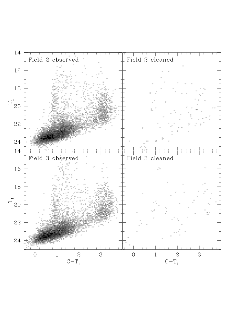
Figure 4: Observed and field star decontaminated Hess diagrams.

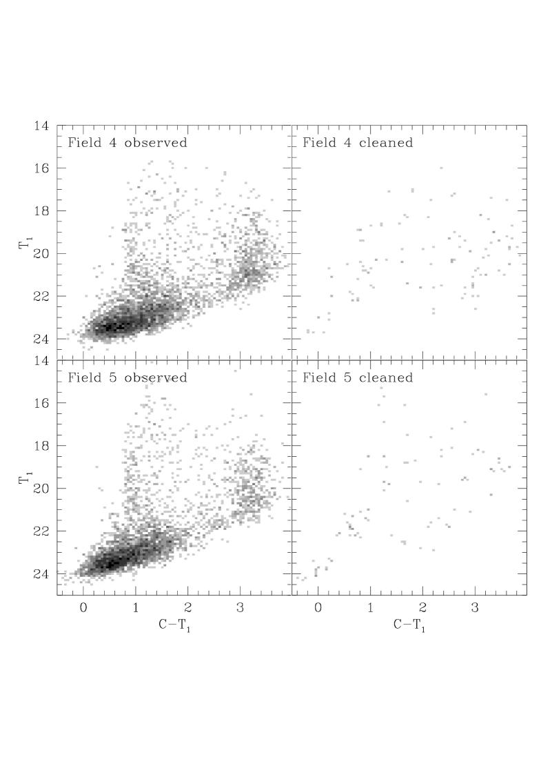
Figure 4: continued.

Hess diagrams have played an increasingly prominent role in the analysis of photometric data, in particular of the Magellanic Clouds. They show the frequency or density of occurrence of stars at various positions on the CMD, thus providing a star density map in the CMD. Hess diagrams have been profitably exploited by using different robust techniques (Harris & Zaritsky, 2001; Dolphin, 2002, and references therein). Here, we simply take advantage of Hess diagrams to identify the prevailing features -in terms of density of stars- and their intrinsic dispersions in the cleaned SMC CMDs. In order to produce these Hess diagrams we counted the number of stars placed in different magnitude-colour bins with sizes [$\Delta$$T_{1}$, $\Delta$$(C-T_{1})$] = (0.1,0.05) mags and then we represented the resultant count scales with a 10 grey levels logarithmic scale. The resultant Hess diagrams for the observed and cleaned SMC CMDs are depicted in a series of panels in Fig. 4.

The cleaned Hess diagrams exhibit different features which tell us about the stellar populations in the surveyed SMC region. A mixture of intermediate-age through old stellar populations clearly appears to be the main feature of these Hess diagrams. Since the SMC field CMDs are obviously composed of stars of different stellar populations, the respective Hess diagrams allow us to recognize the so-called ”dominant populations” (generally darker regions in the Hess diagrams). These stellar populations are the most numerous in a particular region and can be referred as the ”representative” stellar population along the line of sight (LOS) of that SMC field (P12, Piatti & Geisler, 2013; Piatti et al., 2014a). The definition of a representative population could not converge to any dominant population if the stars in a given field came from a constant SFR integrated over all time. For our fields, however, we could clearly identify the respective most populated features. Particularly, the representative MSTOs are in average $\sim$ 1.5 mag brighter than the $T_{1}$ mags for the 100$\%$ completeness level of the respective field, i.e., the faintest $T_{1}$ mag where completeness is still 100$\%$. Therefore, we actually reach the MSTO of the representative population of each field with a negligible loss of stars at that magnitude.

The most distant MS populations from the SMC centre detected by our photometry are located at an angular distance of $\sim$ 5.7$\degr$ (Field 7), equivalent to 6.1 kpc if the SMC distance modulus of 18.96 mag is adopted (de Grijs & Bono, 2015). The adopted optical SMC centre is : 00^h 52^m 45^s, $-$72$\degr$ 49$\arcmin$ 43$\arcsec$ (J2000) (Crowl et al., 2001). We did not find any visible sign of farther clear SMC MS other than the residuals from the MW/background contamination. The resulting SMC radius is in very good agreement with those obtained by Noël & Gallart (2007, $\sim$ 6.3 kpc) from $BV$ photometry of 3 SMC fields and by De Propris et al. (2010, $\sim$ 6 kpc) from Ca II triplet spectroscopy of giant stars, among others. However, it results shorter than the SMC peripheral boundary estimated by Nidever et al. (2011, $\sim$ 10.7 kpc). Their data cover a much larger area of the SMC, which allowed them from the analysis of the giant stellar component to find evidence for a break population beyond $\sim$ 8 kpc with a shallow radial density profile that could be either a bound stellar halo or a population of extratidal stars. In this context, our results confirm that the bulk of the SMC population is contained within $\sim$ 7 deg from the galaxy centre, independently of any possible dependence of the SMC extent with the position angle, beyond which there is a low density envelope extending further out found by (Nidever et al., 2011). Note additionally that some previous studies have suggested the existence of different asymmetries in the SMC (e.g. Subramanian & Subramaniam, 2012; Cignoni et al., 2013; Rubele et al., 2015). Nevertheless, we also carried out counts of red giant clump stars within the box ($\Delta$($C-T_{1}$),$\Delta$($T_{1}$)) = (0.95$-$1.70, 17.90$-$19.70) in the cleaned and observed CMDs. The results are depicted in Fig. 5, where we added a constant to the counts in the cleaned CMDs for comparison purposes and indicated the count level for the outermost field Field 1 (at 12.8 deg, equivalent to 13.8 kpc) with an horizontal line. The uncertainties introduced by both the errors in the relative SMC field reddening and in the photometry are much smaller than the symbol size. The similar shape of both profiles tell us about the robustness of the cleaning procedure, since a similar number of stars was subtracted from each field, once they were properly corrected by incompleteness and reddening effects. On the other hand, the profiles show that the SMC red clump star population that our analysis is able to detect would not appear to extend beyond $\sim$ 6$-$7 deg ($\sim$ 6.6$-$7.7 kpc).

4 Analysis

We used the cleaned CMDs and Hess diagrams of Fields 7 to 11 to constrain the fundamental SMC field parameters by matching the observations with the theoretical isochrones of Bressan et al. (2012) and by using the new age$-$metallicity diagnostic diagram for the Washington photometric system (Piatti & Perren, 2015).

The estimation of the mean SMC field reddening values was made by taking advantage of the NASA/IPAC Extragalactic Data base (NED) to obtained Galactic foreground reddening values for the SMC field list. We adopted the recent recommendation for the mean SMC distance modulus $(m-M)_{0}$ = 18.96 mag, whose formal uncertainty is 0.02 mag but can reach 0.15-0.20 mag if the complex SMC geometry is particularly considered (de Grijs & Bono, 2015). Bearing in mind a 1$\sigma$ LOS depth of 6 kpc Deb et al. (2015), we found that the difference in apparent distance moduli could be as large as $\Delta(T_{1}-M_{T_{1}})$ $\sim$ 0.2 mag. This difference is smaller than the difference between two closely spaced isochrones as used here ($\Delta$ log($t$ yr^-1) = 0.1, $\Delta$($M_{T_{1}}$ at the MSTO-subgiant branch region) $\sim$ 0.3 mag), so that adoption of a unique value for the distance modulus does not dominate the final error budget incurred in matching isochrones to the SMC field Hess diagrams.

We used the ridge lines of the representative SMC field MSs in the Hess diagrams (darker places) to properly find the theoretical isochrones which best superimpose on them. As for the metallicity, we used the values derived from the new age$-$metallicity diagnostic diagram based on the magnitude difference between the red giant clump and the MSTO (Piatti & Perren, 2015, see their fig. 4). We assigned the age of such isochrones to the representative ages of each SMC field. Table 3 lists the derived representative ages and metallicities and their dispersions. The age dispersions have been estimated bearing in mind the broadness in magnitude and colour of the dominant MSs, which represent in general a satisfactory estimate of the age spread around the prevailing population. The metallicity dispersions come from the estimated spread in magnitude of the red clump and the MSTO. Fig. 6 depicts the cleaned Hess diagrams with three different theoretical isochrones superimposed for comparison purposes.

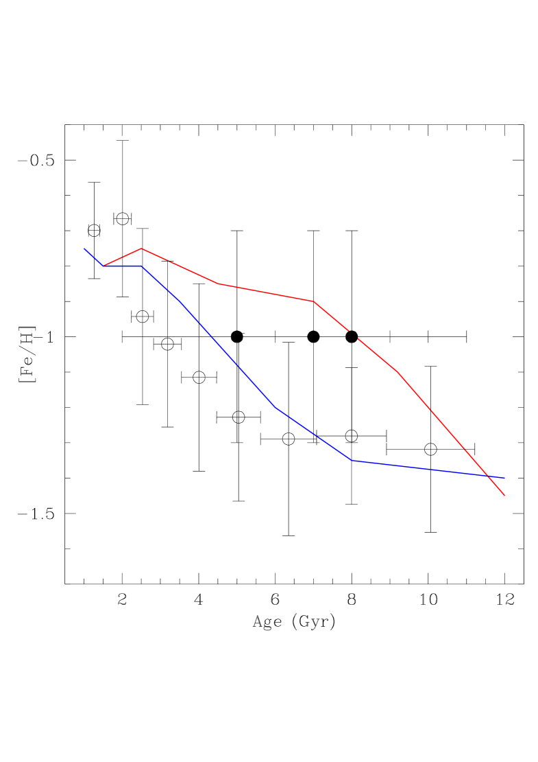
Figure 7: AMR for the presently studied SMC star fields (solid circles), with the dispersion in age and in metallicity represented by errorbars. The mean AMRs by Carrera et al. (2008, red line), Noël et al. (2009, blue line) and Piatti & Geisler (2013, open circles with errorbars) are overplotted.

The derived representative ages and metallicities suggest a constant metallicity level ([Fe/H]= -1.0 dex) and an approximately constant age value ($\approx$ 7-8 Gyr) for the western SMC periphery. We plot these values in Fig. 7 with solid circles, whereas we represent their dispersions with errorbars. Note that the youngest age (5 Gyr) correspond to Field 11, which is located within the SMC main body. Similar age/metallicity values were found by Carrera et al. (2008) from Ca II triplet spectroscopy of giants in 4 fields located towards the western side of the SMC main body, as well as by Noël et al. (2009) who studied 12 SMC star fields from $BR$ photometry (see Fig. 7). The present AMR does not clearly differ from that obtained by P12 for the SMC main body using the same techinques, reproduced by open circles in Fig. 7. The mean SMC AMR derived by P12 is in an overall very good agreement with those obtained by Cignoni et al. (2013, see their fig. 14 and discussions therein), Rubele et al. (2015, see their fig. 17 and discussions therein), among others.

We did not find in the western SMC periphery dominant stellar populations older than $\sim$ 10 Gyr, but a peak centred at $\sim$ 7-8 Gyr. This peak is in excellent agreement with the SFRs recovered by Carrera et al. (2008); Noël et al. (2009); Cignoni et al. (2013) and Rubele et al. (2015, see their fig. 16), who also showed a low initial SFR at $\sim$ 10 Gyr. Particularly, Rubele et al. (2015) showed that the stellar mass formation -measured as the relative to the total galaxy mass ratio- reached a peak $\sim$ 8 Gyr ago. In this context, it seems that the western SMC periphery does not distinguish itself from the major formation processes that took place during the galaxy formation epoch.

5 Conclusions

We have study the western SMC periphery from Washington $CT_{1}$ photometry of eleven star fields (36$\times$36 arcmin² each) covering angular distances to the SMC centre from 2 up to $\sim$ 13 degrees ($\approx$ 2.2 $-$ 13.8 kpc). Our photometric database reaches the 50$\%$ completeness level $\sim$ 2$-$3 mag below the oldest SMC MSTOs, depending on the crowding.

We cleaned the noticeable MW/background field contamination present in the observed SMC star field CMDs using a procedure which makes use of boxes of variable side centred on every star in the MW/background CMD, in order to tightly reproduce it in terms of stellar density, luminosity function and colour distribution. We subtracted the stars in the SMC CMDs that fall within the defined boxes and are closest to the defined box centres.

From the cleaned CMDs (and hence the respective Hess diagrams) we identified the representative (most numerous) stellar populations of each field. Particularly, the most distant representative MS populations from the SMC centre detected by our photometry are located at an angular distance of $\sim$ 5.7 deg (6.1 kpc); no sign of farther SMC MS stars is visible other than the residuals from the MW contamination.

The derived representative ages and metallicities suggest a constant metallicity level ([Fe/H] = -1.0 dex) and an approximately constant age ($\approx$ 7$-$8 Gyr) for the composite stellar population of the western SMC periphery. These values do not clearly differ from those of the most comprehensive AMRs derived for almost the entire SMC main body.

Finally, the range of ages of the representative stellar populations in the western SMC periphery confirm previous results about the major star formation processes from which the galaxy was born. Indeed, after a low SFR at $\sim$ 10 Gyr, the SMC experienced its first significative star formation activity period which peaked $\sim$ 7-8 Gyr ago.

Table 1: Star fields in the SMC.

Field	$\alpha$2000	$\delta$2000	l	b	Filter	Exposure	Airmass	Seeing
	(hms)	($\degr$ $\arcmin$ $\arcsec$)	($\degr$)	($\degr$)	(mag)	(s)		(arcsec)
1	22 35 28	$-$67 06 42	320.8	-45.0	$C$	1$\times$60 + 1$\times$300 + 3$\times$1080	1.25-1.27	1.3-1.6
					$R$	1$\times$10 + 1$\times$50 + 3$\times$580	1.25-1.26	1.3-1.6
2	22 52 43	$-$68 05 45	318.2	-45.4	$C$	1$\times$60 + 1$\times$300 + 3$\times$1080	1.27-1.28	1.0-1.6
					$R$	1$\times$10 + 1$\times$50 + 3$\times$580	1.28-1.30	1.0-1.2
3	23 03 52	$-$69 18 00	316.0	-45.0	$C$	1$\times$60 + 1$\times$300 + 3$\times$1080	1.29-1.32	1.1-1.3
					$R$	1$\times$10 + 1$\times$50 + 3$\times$580	1.29	0.9-1.0
4	23 25 00	$-$70 24 00	313.0	-45.0	$C$	1$\times$60 + 1$\times$300 + 3$\times$1080	1.40-1.52	1.3-1.5
					$R$	2$\times$580	1.54-1.56	1.2
5	23 32 08	$-$70 41 27	312.1	-45.0	$C$	1$\times$60 + 3$\times$1080	1.38-1.46	1.4-1.6
					$R$	1$\times$10 + 3$\times$580	1.32	1.1-1.3
6	0 04 31	$-$66 22 33	310.2	-50.1	$C$	1$\times$60 + 1$\times$300 + 3$\times$1080	1.24-1.25	1.3-1.6
					$R$	1$\times$10 + 1$\times$50 + 3$\times$580	1.24-1.26	1.0-1.2
7	23 55 20	$-$69 28 35	310.1	-46.9	$C$	1$\times$60 + 1$\times$300 + 3$\times$1080	1.43-1.60	1.0-1.2
					$R$	1$\times$10 + 1$\times$50 + 3$\times$580	1.40-1.45	1.1-1.3
8	23 55 00	$-$71 20 00	309.1	-45.1	$C$	1$\times$60 + 1$\times$300 + 3$\times$1080	1.33-1.34	1.2-1.3
					$R$	1$\times$10 + 1$\times$50 + 3$\times$580	1.35-1.38	0.9-1.0
9	0 04 02	$-$70 59 48	308.4	-45.6	$C$	1$\times$60 + 1$\times$300 + 3$\times$1080	1.34-1.38	1.0-1.3
					$R$	1$\times$10 + 1$\times$50 + 3$\times$580	1.32-1.33	1.2-1.4
10	23 41 16	$-$73 08 22	309.8	-43.0	$C$	1$\times$60 + 1$\times$300 + 3$\times$1080	1.37-1.41	1.5-1.7
					$R$	1$\times$10 + 1$\times$50 + 2$\times$580	1.37	1.0
11	0 43 21	$-$70 54 00	303.9	-46.2	$C$	1$\times$60 + 1$\times$300 + 4$\times$1080	1.32-1.34	1.4-1.6
					$R$	1$\times$10 + 1$\times$50 + 3$\times$580	1.40-1.45	1.1-1.3

Table 2: $CT_{1}$ data of stars in Field 1.

Star	$\alpha$2000	$\delta$2000	$T_{1}$	$\sigma$($T_{1}$)	$C-T_{1}$	$\sigma$$(C-T_{1})$	n
	(h:m:s)	($\degr$ $\arcmin$ $\arcsec$)	(mag)	(mag)	(mag)	(mag)
-	-	-	-	-	-	-
124	22:32:29.120	-67:23:03.58	18.130	0.003	1.037	0.006	5
125	22:33:54.381	-67:23:13.03	15.868	0.003	1.338	0.004	5
126	22:33:32.216	-67:23:10.47	19.910	0.007	2.719	0.073	4
-	-	-	-	-	-	-

Table 3: Fundamental properties of studied SMC fields.

Field	$E(B-V)$	angular	age	[Fe/H]
	(mag)	distance (deg)	(Gyr)	(dex)
1	0.024	12.8	$-$	$-$
2	0.026	10.9	$-$	$-$
3	0.029	9.4	$-$	$-$
4	0.037	7.3	$-$	$-$
5	0.034	6.6	$-$	$-$
6	0.018	7.7	$-$	$-$
7	0.027	5.7	8$\pm$2	-1.0$\pm$0.3
8	0.029	4.7	8$\pm$2	-1.0$\pm$0.3
9	0.028	4.2	8$\pm$3	-1.0$\pm$0.3
10	0.027	5.2	7$\pm$2	-1.0$\pm$0.3
11	0.033	2.1	5$\pm$3	-1.0$\pm$0.3

Figure 2: Gray-scale completeness fraction for the crowdest field in our sample (Field 11). The higher the completeness fraction the darker the CMD. Red and blue regions represent the 100% and 50% completeness levels, respectively.

Figure 3: CMDs of stars measured in SMC fields.

Figure 4: continued.

Figure 4: continued.

Figure 4: continued.

Figure 5: Counts of red giant clump stars within the box ($\Delta$($C-T_{1}$),$\Delta$($T_{1}$)) = (0.95$-$1.70, 17.90$-$19.70) in the cleaned (red circle) and observed (open circle) CMDs of the studied SMC fields in terms of their angular distances to the SMC centre. The former have beed shifted by a constant for comparison purposes. The horizontal line represents the counts level for the outermost studied field (Field 1).

Figure 6: Hess diagrams for studied fields with SMC signatures. Three theoretical isochrones taken from Bressan et al. (2012) were superimposed as reference of the dominant ages and metallicities: magenta, red and yellow lines correspond to (age, [Fe/H]) = (5 Gyr, -1.3 dex), (8 Gyr, -1.0 dex) and (10 Gyr, -0.7 dex), respectively, for Field 7, 8 and 9, and (age, [Fe/H]) = (4 Gyr, -1.3 dex), (6.3 Gyr, -1.0 dex) and (8 Gyr, -0.7 dex), respectively, for Field 10 and 11.

References

- Balbinot et al. (2015) Balbinot E. et al., 2015, MNRAS, 449, 1129
- Bica et al. (2008) Bica E., Bonatto C., Dutra C. M., Santos J. F. C., 2008, MNRAS, 389, 678
- Bressan et al. (2012) Bressan A., Marigo P., Girardi L., Salasnich B., Dal Cero C., Rubele S., Nanni A., 2012, MNRAS, 427, 127
- Canterna (1976) Canterna R., 1976, AJ, 81, 228
- Carrera et al. (2008) Carrera R., Gallart C., Aparicio A., Costa E., Méndez R. A., Noël N. E. D., 2008, AJ, 136, 1039
- Cignoni et al. (2013) Cignoni M., Cole A. A., Tosi M., Gallagher J. S., Sabbi E., Anderson J., Grebel E. K., Nota A., 2013, ApJ, 775, 83
- Crowl et al. (2001) Crowl H. H., Sarajedini A., Piatti A. E., Geisler D., Bica E., Clariá J. J., Santos, Jr. J. F. C., 2001, AJ, 122, 220
- de Grijs & Bono (2015) de Grijs R., Bono G., 2015, ArXiv e-prints
- De Propris et al. (2010) De Propris R., Rich R. M., Mallery R. C., Howard C. D., 2010, ApJ, 714, L249
- Deb et al. (2015) Deb S., Singh H. P., Kumar S., Kanbur S. M., 2015, ArXiv e-prints
- Dolphin (2002) Dolphin A. E., 2002, MNRAS, 332, 91
- Geisler (1996) Geisler D., 1996, AJ, 111, 480
- Harris & Zaritsky (2001) Harris J., Zaritsky D., 2001, ApJS, 136, 25
- Jannuzi, Claver & Valdes (2003) Jannuzi B. T., Claver J., Valdes F., 2003, The NOAO Deep Wide Field Survey MOSAIC Data Reductions, http://www.noao.edu/noao/noaodeep/ReductionOpt/frames.html
- Maia, Piatti & Santos (2014) Maia F. F. S., Piatti A. E., Santos J. F. C., 2014, MNRAS, 437, 2005
- Nidever et al. (2011) Nidever D. L., Majewski S. R., Muñoz R. R., Beaton R. L., Patterson R. J., Kunkel W. E., 2011, ApJ, 733, L10
- Noël et al. (2009) Noël N. E. D., Aparicio A., Gallart C., Hidalgo S. L., Costa E., Méndez R. A., 2009, ApJ, 705, 1260
- Noël & Gallart (2007) Noël N. E. D., Gallart C., 2007, ApJ, 665, L23
- Piatti (2011a) Piatti A. E., 2011a, MNRAS, 416, L89
- Piatti (2011b) —, 2011b, MNRAS, 418, L40
- Piatti (2011c) —, 2011c, MNRAS, 418, L69
- Piatti (2012a) —, 2012a, MNRAS, 422, 1109
- Piatti (2012b) —, 2012b, A&A, 540, A58
- Piatti (2014) —, 2014, MNRAS, 440, 3091
- Piatti & Bica (2012) Piatti A. E., Bica E., 2012, MNRAS, 425, 3085
- Piatti et al. (2015) Piatti A. E., de Grijs R., Rubele S., Cioni M. R., Ripepi V., Kerber L., 2015, MNRAS, in press
- Piatti et al. (2014a) Piatti A. E., del Pino A., Aparicio A., Hidalgo S. L., 2014a, MNRAS, 443, 1748
- Piatti & Geisler (2013) Piatti A. E., Geisler D., 2013, AJ, 145, 17
- Piatti, Geisler & Mateluna (2012) Piatti A. E., Geisler D., Mateluna R., 2012, AJ, 144, 100
- Piatti et al. (2014b) Piatti A. E. et al., 2014b, A&A, 570, A74
- Piatti & Perren (2015) Piatti A. E., Perren R., 2015, MNRAS, in press, arXiv:1504.03894
- Robin et al. (2003) Robin A. C., Reylé C., Derrière S., Picaud S., 2003, A&A, 409, 523
- Roderick et al. (2015) Roderick T. A., Jerjen H., Mackey A. D., Da Costa G. S., 2015, ArXiv e-prints
- Rubele et al. (2015) Rubele S. et al., 2015, ArXiv e-prints
- Stetson, Davis & Crabtree (1990) Stetson P. B., Davis L. E., Crabtree D. R., 1990, in Astronomical Society of the Pacific Conference Series, Vol. 8, CCDs in astronomy, Jacoby G. H., ed., pp. 289–304
- Subramanian & Subramaniam (2012) Subramanian S., Subramaniam A., 2012, ApJ, 744, 128
- Weisz et al. (2013) Weisz D. R., Dolphin A. E., Skillman E. D., Holtzman J., Dalcanton J. J., Cole A. A., Neary K., 2013, MNRAS, 431, 364