A Posteriori Error Control
for the Binary Mumford-Shah Model

Abstract

The binary Mumford-Shah model is a widespread tool for image segmentation and can be considered as a basic model in shape optimization with a broad range of applications in computer vision, ranging from basic segmentation and labeling to object reconstruction. This paper presents robust a posteriori error estimates for a natural error quantity, namely the area of the non properly segmented region. To this end, a suitable strictly convex and non-constrained relaxation of the originally non-convex functional is investigated and Repin’s functional approach for a posteriori error estimation is used to control the numerical error for the relaxed problem in the $L^{2}$-norm. In combination with a suitable cut out argument, a fully practical estimate for the area mismatch is derived. This estimate is incorporated in an adaptive meshing strategy. Two different adaptive primal-dual finite element schemes, and the most frequently used finite difference discretization are investigated and compared. Numerical experiments show qualitative and quantitative properties of the estimates and demonstrate their usefulness in practical applications.

1 Introduction

Since the introduction of the image denoising and edge segmentation model by Mumford and Shah in the late 80’s [30], there has been much effort to find effective and efficient numerical algorithms to compute minimizers of different variants of this variational problem. The original model is based on the functional $E_{\text{MS}}[u,K]=\int_{\Omega\backslash K}|\nabla u|^{2}+\alpha(u-u_{0})^{2}{\,\mathrm{d}}x+\beta\mathcal{H}^{n-1}(K)$ with $\alpha,\beta>0$, where $u_{0}:\Omega\to{\mathds{R}}$ is a scalar image intensity on the image domain $\Omega\subset{\mathds{R}}^{n}$, $u$ the reconstructed image intensity and $K$ the associated set of edges, on which the image intensity $u$ jumps. Here, $\mathcal{H}^{n-1}$ denotes the $(n-1)$-dimensional Hausdorff measure. The space of functions of bounded variation $BV(\Omega)$ turned out to be the proper space to formulate the problem in a mathematical rigorous way. Indeed, existence in the context of the space of special functions of bounded variation $SBV(\Omega)$ was proved by Ambrosio (see [3, Theorem 4.2]). For details on these spaces, we refer to [4]. Restricting $u$ to be piecewise constant instead of piecewise smooth, one is lead to a basic and widespread image segmentation model. This model is discussed from a geometric perspective in the book by Morel and Solimini [29]. In the case of just two intensity values $c_{1}$ and $c_{2}$, the associated energy can be rewritten in terms of a characteristic function $\chi\in BV(\Omega,\{0,1\})$ as

$$E[\chi,c_{1},c_{2}]=\int_{\Omega}{\theta}_{1}\chi+{\theta}_{2}(1-\chi){\,\mathrm{d}}x+|{\mathrm{D}}\chi|(\Omega)\,.$$ (1.1)

Here, ${\theta}_{i}=\frac{1}{\nu}(c_{i}-u_{0})^{2}$ for $i=1,2$, the new weight $\nu=\beta/\alpha$ and the resulting binary model is given by $u=c_{1}\chi+c_{2}(1-\chi)$. For fixed $\chi$, one immediately obtains the optimal constants $c_{1}=(\int_{\Omega}\chi{\,\mathrm{d}}x)^{-1}\int_{\Omega}\chi u_{0}{\,\mathrm{d}}x$ and $c_{2}=(\int_{\Omega}1-\chi{\,\mathrm{d}}x)^{-1}\int_{\Omega}(1-\chi)u_{0}{\,\mathrm{d}}x$. For fixed $c_{1}$ and $c_{2}$ one aims at minimizing the energy over the non-convex set of characteristic functions $\chi\in BV(\Omega,\{0,1\})$. Nikolova, Esedoglu and Chan [31] showed that this non-convex minimization problem can be solved via relaxation and thresholding—a breakthrough for both reliable and fast algorithms in computer vision [34, 14]. Here, at first one asks for a minimizer of $E[\cdot,c_{1},c_{2}]$ over all $u\in BV(\Omega,[0,1])$ and then thresholds $u$ for any threshold value $s\in[0,1)$ to obtain the solution $\chi=\chi_{[u>s]}$ of the original minimization problem. The relaxed problem coincides with a constrained version of the classical image denoising model by Rudin, Osher and Fatemi (ROF) [39]. Numerical schemes for an effective and efficient minimization of this model have extensively been studied. Making use of a dual formulation, Chambolle [11] introduced an iterative finite difference scheme and proved its convergence. Hintermüller and Kunisch [26] proposed a predual formulation for a generalized ROF model and proposed to apply a semismooth Newton method for a regularized variant. Chambolle and Pock [17] deduced a primal-dual algorithm with guaranteed first order convergence and applied their approach to different variational models in $BV$ such as image denoising, deblurring and interpolation. The scheme is based on an alternating discrete gradient scheme for the discrete primal and the discrete dual problem. Bartels [6] used the embedding $BV(\Omega)\cap L^{\infty}(\Omega)\hookrightarrow H^{\frac{1}{2}}(\Omega)$ to improve the step-size restriction for $BV$ functionals. Wang and Lucier [41] employed a finite difference approximation of the ROF model and derived an a priori error estimate for the discrete solution based on suitable projection operators. Following Dobson and Vogel [20], the total variation regularization can be approximated smoothly via $\sqrt{|\nabla u|^{2}+\epsilon}$. In [23], the convergence of the $L^{2}$-gradient flow of this smooth approximation to the TV flow in $L^{2}$ is shown under strong regularity assumptions on the solution.

Furthermore, approximations of the original Mumford-Shah model have been studied extensively. An early overview of different approximation and discretization strategies was given by Chambolle in [10]. Ambrosio and Tortorelli [5] proposed a phase field approximation of this functional and proved its $\Gamma$-convergence. Chambolle and Dal Maso [15] proposed a discrete finite element approximation and established its $\Gamma$-convergence. Bourdin and Chambolle [9] picked up this approach and studied the generation of adaptive meshes iteratively adapted in accordance to an anisotropic metric depending on the current approximate solution. In [40], Shen introduced a $\Gamma$-converging approximation of the piecewise constant Mumford-Shah segmentation, where the length term in the Mumford-Shah model is approximated via an approach originating from the phase field model by Modica and Mortola [28]. A simple and widespread level set approach was proposed by Chan and Vese [18].

The goal of this paper is to derive a posteriori error estimates for the binary Mumford-Shah model for fixed constants $c_{1}$ and $c_{2}$. To this end, we proceed as follows: We take into account a suitable strictly convex relaxation of the binary Mumford-Shah functional already studied in [8], which is related to more general relaxation approaches suggested by Chambolle [12] (see Section 2). For this relaxation, we take into account its predual and set up a corresponding primal-dual algorithm [7, 17, 25] (see Section 3). Then, following Bartels [7], we use Repin’s primal-dual approach [36, 37] to derive functional a posteriori error estimates for the relaxed solution based on upper bounds of the duality gap (cf. also the book by Han [24] with respect to mechanical applications) (see Section 4). These estimates can be used together with a suitable cut out argument to derive an a posteriori estimate for the characteristic function $\chi$ minimizing the original functional (1.1) (see Section 5). Moreover, two adaptive finite element discretization schemes and one conventional, non adaptive finite difference scheme are investigated (see Section 6). Finally, we apply the resulting estimate to these schemes incorporating an appropriate post smoothing and present the numerical results (see Sections 7 and 8).

2 A Strictly Convex Relaxation of the Binary Mumford-Shah Model

Henceforth, we use the notation $\chi_{A}$ to denote the indicator function of a measurable set $A\subset\Omega$ and define $[u>c]:=\{x\in\Omega:u(x)>c\}$. Furthermore, we use generic constants $c$ and $C$ throughout this paper. Rewriting the binary Mumford-Shah functional (1.1) as

$$E[\chi,c_{1},c_{2}]=\int_{\Omega}({\theta}_{1}-{\theta}_{2})\chi{\,\mathrm{d}}x+|{\mathrm{D}}\chi|(\Omega)+\int_{\Omega}{\theta}_{2}{\,\mathrm{d}}x\,,$$ (2.1)

one observes that adding a constant to ${\theta}_{1}$ and ${\theta}_{2}$ leaves the minimizers $\chi$ unchanged. Thus, we may assume that ${\theta}_{1},{\theta}_{2}\geq c>0$. Now, let us introduce the following relaxed functional

$$E^{\text{rel}}[u]=\int_{\Omega}u^{2}{\theta}_{1}+(1-u)^{2}{\theta}_{2}{\,\mathrm{d}}x+|{\mathrm{D}}u|(\Omega)\,,$$ (2.2)

which is supposed to be minimized over all $u\in BV(\Omega,{\mathds{R}})$. Indeed, $E^{\text{rel}}[\chi]=E[\chi,c_{1},c_{2}]$ for characteristic functions $\chi$ and one retrieves the original binary Mumford-Shah model. Proving existence of minimizers of (2.2) with the direct method in the calculus of variations is straightforward. For details we refer to [4, 22]. Furthermore, (2.2) is strictly convex by our above assumptions on ${\theta}_{1}$ and ${\theta}_{2}$. Loosely speaking, a preference for the values $0$ and $1$ for $u$ is encoded in the quadratic growing data term. The minimizers of both functionals (1.1) and (2.2) are related in the following sense (cf. [8]):

Proposition 2.1 (Convex relaxation and thresholding).

Under the above assumptions, a minimizer $u\in BV(\Omega)$ of the functional $E^{\text{rel}}$ exists, $u(x)\in[0,1]$ for a.e. $x\in\Omega$ and

$$\chi_{[u>0.5]}\in\operatorname*{argmin}_{\chi\in BV(\Omega,\{0,1\})}E[\chi]\,.$$

Proof.

Proposition 2.1 is an instance of a more general result, which can be found in [12, 16]. In fact, let $\Psi:\Omega\times{\mathds{R}}\rightarrow{\mathds{R}}$ be measurable, $\Psi(\cdot,t)\in L^{1}(\Omega)$ for a.e. $t\in{\mathds{R}}$, $\Psi(x,\cdot)\in C^{1}({\mathds{R}})$ be strictly convex for a.e. $x\in\Omega$, $\Psi(x,t)\geq c|t|-C$ and $E_{\Psi}[u]=\int_{\Omega}\Psi(x,u){\,\mathrm{d}}x+|{\mathrm{D}}u|(\Omega)\,$. Then, there exists a minimizer $u\in\operatorname*{argmin}_{\tilde{u}\in BV(\Omega)}E_{\Psi}[\tilde{u}]$ and for $s\in{\mathds{R}}$

$$\chi^{s}:=\chi_{[u>s]}\in\operatorname*{argmin}_{\chi\in BV(\Omega,\{0,1\})}\int_{\Omega}\partial_{t}\Psi(x,s)\chi{\,\mathrm{d}}x+|{\mathrm{D}}\chi|(\Omega)\,.$$

With $\Psi(x,t)=t^{2}{\theta}_{1}(x)+(1-t)^{2}{\theta}_{2}(x)$ and $s=\frac{1}{2}$ this allows to verify the main claim of Proposition 2.1. Indeed, for $t\in{\mathds{R}}$ and $\chi\in BV(\Omega,\{0,1\})$, let $E^{\text{rel}}_{t}[\chi]:=\int_{\Omega}\partial_{t}\Psi(x,t)\chi{\,\mathrm{d}}x+|{\mathrm{D}}\chi|(\Omega)$. For our specific choice of $\Psi$, $E^{\text{rel}}_{t}[\chi]=\int_{\Omega}\left(2t({\theta}_{1}(x)+{\theta}_{2}(x))-2{\theta}_{2}(x)\right)\chi{\,\mathrm{d}}x+|{\mathrm{D}}\chi|(\Omega)\,$ implies that minimizing the functional $E^{\text{rel}}_{\frac{1}{2}}$ is equivalent to minimizing the functional $E[\cdot,c_{1},c_{2}]$ because $E^{\text{rel}}_{\frac{1}{2}}[\chi]=E[\chi,c_{1},c_{2}]-\int_{\Omega}{\theta}_{2}{\,\mathrm{d}}x$.

For the sake of completeness, we give here the proof of the more general statement tailored to our particular instance. Obviously, $E^{\text{rel}}[\min\{\max\{0,v\},1\}]\leq E^{\text{rel}}[v]$ for any $v\in BV(\Omega)$. Hence, the minimizer takes values in the range $[0,1]$. Due to Fubini’s Theorem, we obtain

$$\int_{\Omega}\Psi(x,u){\,\mathrm{d}}x=\int_{\Omega}\Psi(x,0){\,\mathrm{d}}x+\int_{0}^{1}\int_{\Omega}\partial_{t}\Psi(x,t)\chi_{[u>t]}{\,\mathrm{d}}x{\,\mathrm{d}}t$$

for $u\in BV(\Omega,[0,1])$. For $s\in{\mathds{R}}$, let $\chi^{s}$ denote a minimizer of $E^{\text{rel}}_{s}$ in the set $BV(\Omega,\{0,1\})$. Using the coarea formula (see [4, Theorem 3.40]) and the minimization property of $\chi^{s}$ we get $E^{\text{rel}}[u]\geq C_{\Psi}+\int_{0}^{1}{E^{\text{rel}}_{s}}\left[\chi^{s}\right]{\,\mathrm{d}}s\,,$ where $C_{\Psi}=\int_{\Omega}\Psi(x,0){\,\mathrm{d}}x$.

Next, we make use of the following monotonicity result [2, Lemma 4]: Let $h_{1},h_{2}\in L^{1}(\Omega)$ such that $h_{1}\leq h_{2}$ a.e. in $\Omega$ and assume $\chi_{i}$ is a minimizer of $\int_{\Omega}h_{i}\chi{\,\mathrm{d}}x+|{\mathrm{D}}\chi|(\Omega)$ in $BV(\Omega,\{0,1\})$ for $i\in\{1,2\}$, then $\chi_{1}\geq\chi_{2}$ a.e. in $\Omega$. Due to the strict positivity of ${\theta}_{1}$ and ${\theta}_{2}$ we obtain that $\partial_{t}\Psi(x,s)$ is strictly increasing in $s$ for fixed $x$. Thus, choosing $h_{i}=\partial_{t}\Psi(x,s_{i})$ we get that $\chi^{s_{1}}\geq\chi^{s_{2}}$ a.e. in $\Omega$ for $s_{1}\leq s_{2}$. This implies that $u^{\ast}(x)=\sup\{s\,|\,\chi^{s}(x)=1\}$ is well-defined and Lebesgue measurable with $\chi^{s}=\chi_{[u^{\ast}>s]}$. Furthermore, by the coarea formula we get $u^{\ast}\in BV(\Omega)$ and $C_{\Psi}+\int_{0}^{1}{E^{\text{rel}}_{s}}[\chi^{s}]{\,\mathrm{d}}s=E^{\text{rel}}[u^{*}]\,$. Altogether, we obtain the chain of estimates

$$E^{\text{rel}}[u]\geq C_{\Psi}+\int_{0}^{1}{E^{\text{rel}}_{s}}\left[\chi^{s}\right]{\,\mathrm{d}}s=E^{\text{rel}}[u^{*}]\geq E^{\text{rel}}[u]\,,$$

in which the inequalities are actually equalities. Thus, for a.e. $s\in[0,1]$ the characteristic function $\chi_{[u^{\ast}>s]}$ is a minimizer of ${E^{\text{rel}}_{s}}$. We are left to show that this holds in particular for $s=\tfrac{1}{2}$. To this end, we consider a monotonously decreasing sequence $s_{n}$, which converges to $\tfrac{1}{2}$. For any $\tilde{\chi}\in BV(\Omega,\{0,1\})$ we can infer by the dominated convergence theorem and the weak-$*$ lower semicontinuity of the total variation (noting that $\chi_{[u>s_{n}]}$ converges weak-$*$ in $BV$ to $\chi_{[u>\frac{1}{2}]}$)

$$E^{\text{rel}}_{\frac{1}{2}}[\tilde{\chi}]=\liminf_{n\rightarrow\infty}E^{\text{rel}}_{s_{n}}[\tilde{\chi}]\geq\liminf_{n\rightarrow\infty}E^{\text{rel}}_{s_{n}}[\chi_{[u>s_{n}]}]\geq{E^{\text{rel}}_{s}}[\chi_{[u>\frac{1}{2}]}]\,,$$

from which the assertion follows (indeed the more general result holds by the same argument for all $s\in[0,1)$). ∎

3 A Primal Dual Approach for the Relaxed Problem

In this section, we make use of convex analysis to derive a duality formulation for the minimization problem of the relaxed functional (2.2). Primal and dual formulation will later be used in the a posteriori estimates. The dual of $BV(\Omega)$ is very difficult to characterize and not suitable for computational purposes. Thus, for a generalized ROF model, Hintermüller and Kunisch [25] proposed to consider the corresponding $BV$ functional as the dual of another functional, which we refer to as the predual functional. Bartels [7] made use of this approach in the context of a posteriori estimates for the ROF model. Here, we follow this procedure and investigate the predual of (2.2).

Recall that the Fenchel conjugate $J^{*}$ of a functional $J:X\to\bar{\mathds{R}}$ on a Banach space $X$ with $\bar{\mathds{R}}={\mathds{R}}\cup\{\infty\}$ is a functional on the dual space $X^{\prime}$ with values in $\bar{\mathds{R}}$, defined as $J^{*}[x^{\prime}]=\sup_{x\in X}\{\langle x^{\prime},x\rangle-J[x]\}\,$, where $\langle\cdot,\cdot\rangle$ denotes the duality pairing. Furthermore, we denote by $\Lambda^{*}\in\mathcal{L}(Y^{\prime},X^{\prime})$ the adjoint operator of $\Lambda\in\mathcal{L}(X,Y)$ and by $\partial J$ the subgradient of $J$ (cf. [21]).

Now, we investigate an energy functional

$${D^{\text{rel}}}[q]=F[q]+G[\Lambda q]\qquad q\in\mathcal{Q}\,,$$ (3.1)

where $F:\mathcal{Q}\rightarrow\bar{\mathds{R}}$ and $G:\mathcal{V}\rightarrow\bar{\mathds{R}}$ being proper, convex and lower semicontinuous functionals, $\mathcal{V}$ and $\mathcal{Q}$ being reflexive Banach spaces and $\Lambda\in\mathcal{L}(\mathcal{Q},\mathcal{V})$. In our case of the predual of the convex relaxed binary Mumford-Shah model, we have

$$F[q]=I_{\overline{B}_{1}}[q]=\left\{\begin{array}[]{c l}0&\text{if }|q|\leq 1\text{ a.e.}\\ +\infty&\text{else}\end{array}\right.\,,\quad G[v]=\int_{\Omega}\frac{\frac{1}{4}v^{2}+v{\theta}_{2}-{\theta}_{1}{\theta}_{2}}{{\theta}_{1}+{\theta}_{2}}{\,\mathrm{d}}x\,,$$

with $\Lambda=\operatorname{div}$, $\mathcal{Q}=H_{N}(\operatorname{div},\Omega)$ and $\mathcal{V}=L^{2}(\Omega)$. Recall the definition of the spaces $H(\operatorname{div},\Omega)=\{q\in L^{2}(\Omega,\mathbb{R}^{n}):\ \operatorname{div}q\in L^{2}(\Omega)\}$, endowed with the norm $\|q\|_{H(\operatorname{div},\Omega)}^{2}=\|q\|_{L^{2}(\Omega)}^{2}+\|\operatorname{div}q\|_{L^{2}(\Omega)}^{2}$, and $H_{N}(\operatorname{div},\Omega)=H(\operatorname{div},\Omega)\cap\{q\cdot\nu=0\text{ on }\partial\Omega\}$, where $\nu$ is the outer normal on $\partial\Omega$ and the operator $\operatorname{div}$ is understood in the weak sense. Moreover, $\Lambda^{*}=-\nabla$ holds in the sense

$$(\Lambda^{*}v,q)_{L^{2}(\Omega)}=(v,\operatorname{div}q)_{L^{2}(\Omega)}\quad\forall v\in\mathcal{V},\ q\in\mathcal{Q}\,.$$

Based on this duality and for the particular choice of ${D^{\text{rel}}}$, we easily verify that $({D^{\text{rel}}})^{\ast}=E^{\text{rel}}$. Indeed, from the general theory in [21, pp. 58 ff.], we can deduce $({D^{\text{rel}}})^{\ast}[v]=F^{*}[-\Lambda^{*}v]+G^{*}[v]$. As a result of the denseness of $C^{1}_{c}(\Omega)$ in $H_{N}(\operatorname{div},\Omega)$ with respect to the norm $\|\cdot\|_{H(\operatorname{div},\Omega)}$, we can infer for any $v\in BV(\Omega)$

$$|{\mathrm{D}}v|(\Omega)=\sup_{q\in\mathcal{Q},\|q\|_{\infty}\leq 1}\int_{\Omega}v\operatorname{div}q{\,\mathrm{d}}x=\sup_{q\in\mathcal{Q}}\left(-\int_{\Omega}v\operatorname{div}q{\,\mathrm{d}}x-I_{\overline{B}_{1}}[q]\right)\,,$$

which leads to

$$F^{*}[-\Lambda^{*}v]=\sup_{q\in\mathcal{Q}}\left(-\int_{\Omega}v\operatorname{div}q{\,\mathrm{d}}x-I_{\overline{B}_{1}}[q]\right)=|{\mathrm{D}}v|(\Omega)\,.$$

On the other hand, the Fenchel conjugate of $G$ can be computed as follows:

$$G^{*}[v]=\sup_{w\in L^{2}(\Omega)}\left((v,w)_{L^{2}(\Omega)}-G[w]\right)=\int_{\Omega}v^{2}{\theta}_{1}+(1-v)^{2}{\theta}_{2}{\,\mathrm{d}}x\,,$$

where the supremum is attained for $w=2v({\theta}_{1}+{\theta}_{2})-2{\theta}_{2}$. This verifies the assertion.

Now, the central insight is that

$${D^{\text{rel}}}[p]=-({D^{\text{rel}}})^{\ast}[u]$$ (3.2)

for a minimizer $p$ of ${D^{\text{rel}}}$ and a minimizer $u$ of $({D^{\text{rel}}})^{\ast}$. This can be seen by formally exchanging $\inf$ and $\sup$ as follows

$${D^{\text{rel}}}[p]= \inf_{q\in H_{N}(\operatorname{div},\Omega)}(F[q]+G[\Lambda q])=\inf_{q\in H_{N}(\operatorname{div},\Omega)}\sup_{v\in L^{2}(\Omega)}(F[q]+\langle v,\Lambda q\rangle-G^{*}[v])$$

$$= \!\!\sup_{v\in L^{2}(\Omega)}\!\left(-\!\!\!\!\!\sup_{q\in H_{N}(\operatorname{div},\Omega)}\!\!(\langle-\Lambda^{*}v,q\rangle-F[q])-G^{*}[v]\right)\!=\!\!\!\sup_{v\in L^{2}(\Omega)}\!\!\!\left(-F^{*}[-\Lambda^{*}v]-G^{*}[v]\right)$$

$$= \!\sup_{v\in L^{2}(\Omega)}(-({D^{\text{rel}}})^{\ast}[v])=-\inf_{v\in L^{2}(\Omega)}({D^{\text{rel}}})^{\ast}[v]=-({D^{\text{rel}}})^{\ast}[u]\,.$$

A rigorous verification can be found in [21, Chapter III.4] (see also [38, 36, 7]). Furthermore, one obtains that $\bar{q}\in\mathcal{Q}$ and $\bar{v}\in\mathcal{V}$ are optimal if and only if $-\Lambda^{*}\bar{v}\in\partial F[\bar{q}]$ and $\bar{v}\in\partial G[\Lambda\bar{q}]$, which can be deduced from the equivalence $J[x]+J^{*}[x^{\prime}]=\langle x^{\prime},x\rangle\Longleftrightarrow x^{\prime}\in\partial J[x]\,$ (see [21, Proposition I.5.1]).

4 Functional A Posteriori Estimates for the Relaxed Problem

In what follows, we investigate a posteriori error estimates associated with the energy ${D^{\text{rel}}}[q]=F[q]+G[\Lambda q]$ and its dual $E^{\text{rel}}[v]=F^{*}[-\Lambda^{*}v]+G^{*}[v]$. A crucial prerequisite is the uniform convexity of $G$, which is linked to the specific choice of the relaxed Model $E^{\text{rel}}$.

Recall that a functional $J:X\rightarrow{\mathds{R}}$ is uniformly convex, if there exists a continuous functional $\Phi_{J}:X\rightarrow[0,\infty)$ such that $J\!\left[\tfrac{x_{1}+x_{2}}{2}\right]+\Phi_{J}(x_{2}-x_{1})\leq\tfrac{1}{2}(J[x_{1}]+J[x_{2}])$ for all $x_{1},x_{2}\in X$ and $\Phi_{J}(x)=0$ if and only if $x=0$. Furthermore, we denote by $\Psi_{J}$ a non-negative functional such that $\langle x^{\prime},x_{2}-x_{1}\rangle+\Psi_{J}(x_{2}-x_{1})\leq J[x_{2}]-J[x_{1}]$ for all $x^{\prime}\in\partial J[x_{1}]\,.$ Hence, $\Psi_{J}$ allows a quantification of the strict monotonicity of $J$. If $J\in C^{2}$ and $\lambda_{min}$ denotes the smallest eigenvalue of $D^{2}J[0]$, then $\Phi_{J}$ and $\Psi_{J}$ admit the representation

$$\Phi_{J}(x)=\frac{1}{8}\lambda_{min}(D^{2}J[0])\|x\|^{2}\quad\text{and}\quad\Psi_{J}(x)=\frac{1}{2}\lambda_{min}(D^{2}J[0])\|x\|^{2}\,,$$

which follows readily via a Taylor expansion.

Now, the a posteriori error estimate is based on the following direct application of a general result by Repin [36]: Let $u\in\operatorname*{argmin}_{\tilde{v}\in\mathcal{V}}E^{\text{rel}}[\tilde{v}]$ and $q\in\mathcal{Q}$, $v\in\mathcal{V}^{\prime}=\mathcal{V}=L^{2}(\Omega)$. Then,

$$\Phi_{G^{*}}(u-v)+\Phi_{F^{*}}(\Lambda^{*}(u-v))+\Psi_{E^{\text{rel}}}\!\left(\frac{u-v}{2}\right)\leq\frac{1}{2}(E^{\text{rel}}[v]+{D^{\text{rel}}}[q])\,.$$ (4.1)

The proof of (4.1) relies on the following two estimates: At first,

$$\Phi_{G^{*}}(u-v)+\Phi_{F^{*}}(\Lambda^{*}(u-v))$$

$$\leq\frac{1}{2}\left(F^{*}[\Lambda^{*}v]+G^{*}[v]+F^{*}[\Lambda^{*}u]+G^{*}[u]\right)-\left(F^{*}\!\left[\Lambda^{*}\frac{u+v}{2}\right]+G^{*}\!\left[\frac{u+v}{2}\right]\right)\,,$$

which is a consequence of the uniform convexity. Secondly, using the monotonicity and that $u$ is a minimizer of $E$ and thus $0\in\partial E^{\text{rel}}[u]$, we get

$$\Psi_{E^{\text{rel}}}\!\left(\frac{u-v}{2}\right)\leq F^{*}\!\left[\Lambda^{*}\frac{u+v}{2}\right]+G^{*}\!\left[\frac{u+v}{2}\right]-\left(F^{*}[\Lambda^{*}u]+G^{*}[u]\right).$$

The claim follows by adding both estimates and using the fundamental relation $E^{\text{rel}}[u]\geq-{D^{\text{rel}}}[q]$ known as the weak complementarity principle (cf. [21, 36, 7]). In the case of the binary Mumford-Shah model, we easily compute

$$\Phi_{F^{*}}\equiv 0,\ \Phi_{G^{*}}(v)=\frac{1}{4}\int_{\Omega}v^{2}({\theta}_{1}+{\theta}_{2}){\,\mathrm{d}}x,\ \Psi_{E^{\text{rel}}}(v)=\int_{\Omega}v^{2}({\theta}_{1}+{\theta}_{2}){\,\mathrm{d}}x$$

and the estimate (4.1) implies for any $v\in\mathcal{V}$ and $q\in\mathcal{Q}$

$$\int_{\Omega}(u-v)^{2}({\theta}_{1}+{\theta}_{2}){\,\mathrm{d}}x\leq E^{\text{rel}}[v]+{D^{\text{rel}}}[q]\,.$$

Finally, $\frac{1}{2}(a-b)^{2}\leq a^{2}+b^{2}$ with $a=c_{1}-u_{0}$ and $b=c_{2}-u_{0}$ yields $\frac{1}{2\nu}(c_{1}-c_{2})^{2}\leq{\theta}_{1}+{\theta}_{2}$. Thus, we obtain the following theorem:

Theorem 4.1.

Let $u\in\mathcal{V}$ be the minimizer of $E^{\text{rel}}$. Then, for any $v\in\mathcal{V}$ and $q\in\mathcal{Q}$ it holds that

$$\|u-v\|_{L^{2}(\Omega)}^{2}\leq\mathrm{err}_{u}^{2}[v,q]:=\frac{2\nu}{(c_{1}-c_{2})^{2}}\left(E^{\text{rel}}[v]+{D^{\text{rel}}}[q]\right)\,.$$ (4.2)

In the application, one asks for (post processed) discrete primal $v$ and dual solution $q$ which ensure a small right hand side. Additionally, the estimator $\mathrm{err}_{u}$ is consistent, i.e. $\mathrm{err}_{u}[v,q]\rightarrow 0$ provided $v$ and $q$ converge to the extrema of the corresponding energy functionals w.r.t. the topology of the associated Banach spaces.

5 A Posteriori Error Estimates for the Binary Mumford-Shah Model

In the sequel, we expand the a posteriori theory to the binary Mumford-Shah model. The key observation is that for many images approximate solutions $u\in L^{2}(\Omega)$ of the relaxed model are characterized by steep profiles, where the actual solution of the original binary Mumford-Shah model jumps. Thus, we proceed as follows. We define

$$\mathrm{a}[v,\eta]=\left\|\chi_{[\frac{1}{2}-\eta\leq v\leq\frac{1}{2}+\eta]}\right\|_{L^{1}(\Omega)}$$

for $\eta\in\left(0,\tfrac{1}{2}\right)\,$, which measures the area of the preimage of the interval of size $2\eta$ centered at the threshold value $s=\tfrac{1}{2}$ (cf. Section 2). Based on the above observation, the set $\mathcal{S}_{\eta}=\left[\tfrac{1}{2}-\eta\leq v\leq\tfrac{1}{2}+\eta\right]$ can be regarded as the set of non properly identified phase. Taking into account this definition, we obtain the following theorem.

Theorem 5.1 (A posteriori error estimator for the binary Mumford-Shah model).

For fixed $c_{1}$ and $c_{2}$ let $\chi\in BV(\Omega,\{0,1\})$ be a minimizer of the binary Mumford-Shah functional $E[\cdot,c_{1},c_{2}]$ (1.1). Then for all $v\in\mathcal{V}=L^{2}(\Omega)$ and $q\in\mathcal{Q}=H_{N}(\operatorname{div},\Omega)$ we have that

$$\left\|\chi-\chi_{[v>\frac{1}{2}]}\right\|_{L^{1}(\Omega)}\leq\mathrm{err}_{\chi}[v,q]:=\inf_{\eta\in(0,\frac{1}{2})}\left(\mathrm{a}[v,\eta]+\frac{1}{\eta^{2}}\mathrm{err}_{u}^{2}[v,q]\right)\,.$$ (5.1)

Let us remark that $\chi_{[v>\frac{1}{2}]}$ is the result of the same thresholding, which relates $\chi$ to the solution $u$ of the relaxed problem (2.2), i.e. $\chi=\chi_{[u>\frac{1}{2}]}$, this time applied to $v$.

Proof.

Recall that any minimizer $u$ of the $E^{\text{rel}}$ fulfills $0\leq u\leq 1$. For all $\eta\in(0,\tfrac{1}{2})$ we obtain the following set relation for the symmetric difference of the sets $[u>\frac{1}{2}]$ and $[v>\frac{1}{2}]$ ($\Delta$ denoting the symmetric difference of two sets):

$$\left[u>\tfrac{1}{2}\right]\Delta\left[v>\tfrac{1}{2}\right]\subseteq\left\{x\in\Omega\,\big{|}\,\tfrac{1}{2}-\eta\leq v(x)\leq\tfrac{1}{2}+\eta\right\}\cup\left\{x\in\Omega\,\big{|}\,|u-v(x)|>\eta\right\}\,.$$

Now, using Theorem 4.1 the Lebesgue measure of the rightmost set can be estimated as follows

$$\mathcal{L}^{n}(|u-v|>\eta)\leq\int_{\{|u-v|>\eta\}}\frac{|u-v|^{2}}{\eta^{2}}{\,\mathrm{d}}x\leq\frac{1}{\eta^{2}}\mathrm{err}_{u}^{2}[v,q]\,,$$

where $\eta\in(0,\frac{1}{2})$. Finally, taking the infimum for all $\eta\in(0,\tfrac{1}{2})$ concludes the proof. ∎

In the application, the computational cost to find the optimal $\eta$ is of the order of the degrees of freedom for the discrete solution and thus affordable. Let us emphasize that the error estimator $\mathrm{err}_{\chi}$ is not tailored to a specific finite element approach. Indeed, we can project any primal and dual solution onto the spaces $\mathcal{V}=L^{2}(\Omega)$ and $\mathcal{Q}=H_{N}(\operatorname{div},\Omega)$, respectively. We will exploit this in the next sections.

6 Finite Element and Finite Difference Discretization

In this section, we investigate different numerical approximation schemes for the primal and the dual solution of the relaxed problem (2.2) on adaptive meshes and the refinement of the meshes based on the a posteriori error estimate in Theorem 5.1. In the context of image processing applications with input images usually given on a regular rectangular mesh, an adaptive quadtree for $n=2$ (or octree for $n=3$) turned out to be an effective choice for an adaptive mesh data structure. In what follows, we pick up the finite element approach for a variational problem on $BV$ proposed by Bartels [6] and a simplified version of the latter. Furthermore, we consider the widespread finite different scheme proposed by Chambolle [11].

(FE) Finite element scheme on an induced adaptive triangular grid.

We consider $\Omega=[0,1]^{2}$ in all numerical experiments in this paper. On this domain, we consider an adaptive mesh $\mathcal{M}_{h}$ described by a quadtree with cells $\mathscr{C}\in\mathcal{M}_{h}$ being squares, which are recursively refined into four squares via an edge bisection. We suppose that the level of refinement between cells at edges differs at most by one. Thus, on a single edge at most one hanging node appears. Let $h$ indicate the spatially varying mesh size function on $\Omega$, i.e. in the range of an initial mesh size $2^{-L_{\mbox{\tiny init}}}$ and a finest mesh size $2^{-L_{0}}$ (usually determined by the image resolution). For all discretization approaches investigated here, the degrees of freedom are associated with the non hanging nodes. Let us denote by $N_{v}$ the number of these nodes, which will coincide with the number of degrees of freedom of discrete primal functions. The finite element discretization is based on a triangular mesh $\mathcal{S}_{h}$ spread over the adaptive quadtree mesh via a splitting of each quadratic leaf cell into simplices $\mathscr{T}$ ( “cross subdivision”). We ask for discrete primal functions $u_{h}$ in the space of piecewise affine and globally continuous functions on $\mathcal{S}_{h}$ denoted by $\mathcal{V}_{h}$. Thus, for functions $v_{h}\in\mathcal{V}_{h}$ the values at hanging nodes are interpolated based on the values at adjacent non hanging nodes, which are associated with the actual degrees of freedom. By $\mathcal{Q}_{h}=\left\{q_{h}\in\mathcal{V}^{N}_{h}:\ q_{h}\cdot\nu=0\text{ on }\partial\Omega\right\}$ we denote the discrete counterpart of $\mathcal{Q}$. To accommodate this boundary condition, the boundary nodes are modified after each update of the dual solution in a post-processing step. On $\mathcal{V}_{h}$, we define discrete counterparts of the continuous functionals $F$ and $G$ as follows:

$$G_{h}[v_{h}]:=\int_{\Omega}\frac{\frac{1}{4}v_{h}^{2}+v_{h}\theta_{2,h}-\theta_{1,h}\theta_{2,h}}{\theta_{1,h}+\theta_{2,h}}{\,\mathrm{d}}x\,,\quad F_{h}[q_{h}]:=I_{\bar{B}_{1}}[q_{h}]\,,$$

where $\theta_{i,h}=\mathcal{I}_{h}(\theta_{i})=\mathcal{I}_{h}(\tfrac{1}{\nu}(c_{i}-u_{0})^{2})$ for $i=1,2$ with $\mathcal{I}_{h}$ denoting the Lagrange interpolation. In the application on images, we suppose that $u_{0}\in\mathcal{V}_{0}$, where $\mathcal{V}_{0}$ is the simplicial finite element space corresponding to the full resolution image on the finest grid level $L_{0}$ representing the full image resolution. Furthermore, we consider two different scalar products. On $\mathcal{V}_{h}$, we take into account the $L^{2}$-product and on $\mathcal{Q}_{h}$ the lumped mass product $(q_{h},p_{h})\mapsto\int_{\Omega}\mathcal{I}_{h}(q_{h}p_{h}){\,\mathrm{d}}x$ and identify $\mathcal{V}_{h}$ and $\mathcal{Q}_{h}$ with their dual spaces with respect to the $L^{2}$- and the lumped mass product, respectively. Then, the associated dual operators are

$$G_{h}^{\ast}[v_{h}]=\int_{\Omega}v_{h}^{2}\theta_{1,h}+(1-v_{h})^{2}\theta_{2,h}{\,\mathrm{d}}x\,,\quad F_{h}^{\ast}[q_{h}]=\int_{\Omega}\mathcal{I}_{h}(|q_{h}|){\,\mathrm{d}}x\,.$$

Finally, we define the discrete divergence $\Lambda_{h}:\mathcal{Q}_{h}\to\mathcal{V}_{h}$, $q_{h}\mapsto\mathcal{P}_{h}\operatorname{div}q_{h}$, where $\mathcal{P}_{h}$ denotes the $L^{2}$-projection $\mathcal{P}_{h}:L^{2}(\Omega)\rightarrow\mathcal{V}_{h}$. Following Bartels [7] and taking into account the above scalar products on $\mathcal{V}_{h}$ and on $\mathcal{Q}_{h}$, we obtain for the discrete gradient $-\Lambda_{h}^{\ast}:\mathcal{V}_{h}\to\mathcal{Q}_{h}$, $v_{h}\mapsto-\Lambda_{h}^{\ast}v_{h}$, the defining duality

$$\int_{\Omega}\mathcal{I}_{h}(-\Lambda_{h}^{\ast}v_{h}\cdot q_{h}){\,\mathrm{d}}x=\int_{\Omega}v_{h}\mathcal{P}_{h}\operatorname{div}q_{h}{\,\mathrm{d}}x$$ (6.1)

for all $q_{h}\in\mathcal{Q}_{h}$ and $v_{h}\in\mathcal{V}_{h}$.

(FE’) Finite element scheme based on a simple gradient operator.

Instead of the above defined discrete gradient operator $-\Lambda_{h}^{\ast}$, we alternatively consider the piecewise constant gradient $\nabla v_{h}$ on the simplices $\mathscr{T}$ of the simplicial mesh for functions $v_{h}\in\mathcal{V}_{h}$. To this end, we choose $\mathcal{Q}_{h}$ as the space of piecewise constant functions on the simplicial mesh, and take into account the standard $L^{2}$-product on both spaces. The above definitions of the functionals $G_{h}$ and $F_{h}$ are still valid. Moreover, $G^{\ast}_{h}$ remains the same, only $F^{\ast}_{h}$ changes to $F_{h}^{\ast}[q_{h}]=\int_{\Omega}|q_{h}|{\,\mathrm{d}}x$. The discrete divergence $\Lambda_{h}:\mathcal{Q}_{h}\to\mathcal{V}_{h}$ is defined via duality starting from the preset discrete gradient as

$$\int_{\Omega}\mathcal{I}_{h}(\Lambda_{h}q_{h}v_{h}){\,\mathrm{d}}x=-\int_{\Omega}q_{h}\cdot\nabla v_{h}{\,\mathrm{d}}x\,,$$

which indeed ensures that $-\Lambda_{h}^{\ast}v_{h}=\nabla v_{h}$. This simplified ansatz leads to a non-conforming iterative solution scheme (see Section 7), since the space of piecewise constant finite elements is not contained in $H_{N}(\operatorname{div},\Omega)$ (cf. [6]). After each modification of the (piecewise constant) dual solution the values on the corresponding boundary cells are set to $0$ to satisfy the boundary condition. To apply the derived a posteriori error estimates a projection onto the space $H_{N}(\operatorname{div},\Omega)$ is required. To this end, we replace the solution $p_{h}\in\mathcal{Q}_{h}$ by its $L^{2}$-projection onto the space $\mathcal{V}_{h}^{n}$.

(FD) Finite difference scheme on a regular mesh.

The finite difference scheme for the numerical solution of functionals on $BV$ proposed by Chambolle [11] is extensively used in many computer vision applications and applies to image data defined on a structured non adaptive mesh. We compare the a posteriori error estimator for this scheme on non adaptive meshes with the above finite element schemes on adaptive meshes. To this end, we denote by $\mathbf{V}_{h}\in{\mathds{R}}^{N_{v}}$ and $\mathbf{Q}_{h}\in{\mathds{R}}^{2N_{v}}$ nodal vectors on the regular lattice for primal and dual solutions, respectively. Here, $N_{v}=(h^{-1}+1)^{2}$, where $h$ denotes the fixed grid size of the finite difference lattice. Integration is replaced by summation and we obtain the following discrete analogues ${\mathbf{G}_{h}}$ and ${\mathbf{F}_{h}}$ of the continuous functionals $F$ and $G$ as functions on ${\mathds{R}}^{N_{v}}$ and ${\mathds{R}}^{2N_{v}}$, respectively:

$${\mathbf{G}_{h}}[\mathbf{V}_{h}]:=\sum_{i=1}^{N_{v}}\left(\frac{\frac{1}{4}(\mathbf{V}_{h}^{i})^{2}+\mathbf{V}_{h}^{i}{\Theta^{i}_{2,h}}-{\Theta^{i}_{1,h}}{\Theta^{i}_{2,h}}}{{\Theta^{i}_{1,h}}+{\Theta^{i}_{2,h}}}\right)\,,\quad{\mathbf{F}_{h}}[\mathbf{Q}_{h}]:=\max_{i=1,\ldots,N_{v}}\mathbf{I}_{\bar{B}_{1}}[\mathbf{Q}_{h}^{i}]$$

with ${\Theta^{i}_{1,h}}$, ${\Theta^{i}_{2,h}}$ denoting the pointwise evaluation of $\theta_{1}$ and $\theta_{2}$, respectively, and $\mathbf{I}_{\bar{B}_{1}}[\mathbf{Q}_{h}^{i}]=0$ for $|\mathbf{Q}_{h}^{i}|\leq 1$ and $+\infty$ otherwise. The associated dual operators for the standard Euclidean product as the duality pairing are

$${\mathbf{G}^{\ast}_{h}}[\mathbf{V}_{h}]=\sum_{i=1}^{N_{v}}(\mathbf{V}_{h}^{i})^{2}{\Theta^{i}_{1,h}}+(1-\mathbf{V}_{h}^{i})^{2}{\Theta^{i}_{2,h}}\,,\quad{\mathbf{F}^{\ast}_{h}}[\mathbf{Q}_{h}]=\sum_{i=1}^{N_{v}}\left|\mathbf{Q}_{h}^{i}\right|\,.$$

Finally, we take into account periodic boundary conditions (by identifying degrees of freedom on opposite boundary segments) and use forward difference quotients to define the discrete gradient operator $-\mathbf{\Lambda}_{h}^{\ast}:{\mathds{R}}^{N_{v}}\to{\mathds{R}}^{2N_{v}}$, i.e.

$$((-\mathbf{\Lambda}_{h}^{\ast})\mathbf{V}_{h})^{i}=\left(\frac{\mathbf{V}_{h}^{{\mathscr{N}}(i,j)}-\mathbf{V}_{h}^{i}}{h}\right)_{j=1,2}\,,$$

where ${\mathscr{N}}(i,j)$ is the index of the neighboring node in direction of the $j$th coordinate vector. As a consequence, the matrix representing the discrete divergence operator $\mathbf{\Lambda}_{h}:{\mathds{R}}^{2N_{v}}\to{\mathds{R}}^{N_{v}}$ is just the negative transpose of the matrix representing the discrete gradient and thus corresponds to a discrete divergence based on backward difference quotients.

To use the a posteriori error estimate in the finite difference context, we consider as a simplest choice the piecewise bilinear functions $u_{h}$ and $p_{h}$ uniquely defined by the solution vectors $\mathbf{U}_{h}$ and $\mathbf{P}_{h}$, respectively. The boundary condition is taken care of in exactly the same way as in the case (FE).

7 Implementation based on a Primal-Dual Algorithm

For the numerical solution of the different discrete variational problems, we use the primal-dual algorithm proposed by Chambolle and Pock [17, Algorithm 1], which computes both a discrete primal and a discrete dual solution to be used in the a posteriori error estimates. Note that we use [17, Algorithm 1] instead of [17, Algorithm 2] even though ${\mathbf{G}^{\ast}_{h}}$ is uniformly convex. As we will see later, evaluating $(\mathrm{Id}+\tau\partial{\mathbf{G}^{\ast}_{h}})^{-1}$ requires the inversion of a matrix depending on $\tau$. In Algorithm 1, $\tau$ is fixed and the inverse can be computed once using a Cholesky decomposition for the sparse, symmetric and positive-definite matrix (for details see [19]), while in Algorithm 2 the decomposition of the linear system has to be performed in each iteration. Before we discuss this algorithm in the more conventional matrix-vector notation, let us rewrite the finite element approaches correspondingly. Let $N_{v}=\mathrm{dim}\,\mathcal{V}_{h}$ (the number of non hanging nodes) and $N_{q}=\mathrm{dim}\,\mathcal{Q}_{h}$ (for (FE) $N_{q}=2N_{v}$ and for (FE’) $N_{q}$ is $2$ times the number of simplices). In what follows, we will use uppercase letters to denote a vector of nodal values, e.g. $\mathbf{V}_{h}^{i}=v_{h}(X^{i})$ if $X^{i}$ is the $i$th non hanging node. The two scalar products are encoded via mass matrices. Here, ${\mathbf{M}_{h}}\in{\mathds{R}}^{N_{v},N_{v}}$ represents the standard $L^{2}$-product on $\mathcal{V}_{h}$ and is given by ${\mathbf{M}_{h}}\mathbf{V}_{h}\cdot\mathbf{U}_{h}=\int_{\Omega}v_{h}u_{h}{\,\mathrm{d}}x$ for all $v_{h},\,u_{h}\in\mathcal{V}_{h}$. Furthermore, $\mathbf{\tilde{M}}_{h}\in{\mathds{R}}^{N_{q},N_{q}}$ is the mass matrix associated with the space $\mathcal{Q}_{h}$. For the approach (FE) it is given as the lumped mass matrix with $\mathbf{\tilde{M}}_{h}\mathbf{P}_{h}\cdot\mathbf{Q}_{h}=\int_{\Omega}\mathcal{I}_{h}(p_{h}\cdot q_{h}){\,\mathrm{d}}x$ for all $p_{h},\,q_{h}\in\mathcal{Q}_{h}$, whereas for the discretization (FE’) $\mathbf{\tilde{M}}_{h}\mathbf{P}_{h}\cdot\mathbf{Q}_{h}=\int_{\Omega}p_{h}\cdot q_{h}{\,\mathrm{d}}x$ for all $p_{h},\,q_{h}\in\mathcal{Q}_{h}$ defines a classical (diagonal) mass matrix. For the matrix representations $\mathbf{\Lambda}_{h}$ and $-\mathbf{\Lambda}_{h}^{\ast}$ of the discrete divergence and the discrete gradient, respectively, we obtain the relation (cf. [7])

$$\mathbf{\Lambda}_{h}^{\ast}=\mathbf{\tilde{M}}_{h}^{-1}\mathbf{\Lambda}_{h}^{T}{\mathbf{M}_{h}}\,.$$ (7.1)

For the discretization (FD) we have $\mathbf{\Lambda}_{h}^{\ast}=\mathbf{\Lambda}_{h}^{T}$. Altogether, the discrete predual energy ${\mathbf{D}_{h}^{rel}}:{\mathds{R}}^{N_{q}}\to{\mathds{R}}$ and the discrete energy ${\mathbf{E}_{h}^{rel}}:{\mathds{R}}^{N_{v}}\to{\mathds{R}}$ are defined as follows:

$${\mathbf{D}_{h}^{rel}}[\mathbf{Q}_{h}]={\mathbf{F}_{h}}[\mathbf{Q}_{h}]+{\mathbf{G}_{h}}[\mathbf{\Lambda}_{h}\mathbf{Q}_{h}]\,,\quad{\mathbf{E}_{h}^{rel}}[\mathbf{V}_{h}]={\mathbf{F}^{\ast}_{h}}[-\mathbf{\Lambda}_{h}^{\ast}\mathbf{V}_{h}]+{\mathbf{G}^{\ast}_{h}}[\mathbf{V}_{h}]\,.$$

In the case of both finite element schemes ${\mathbf{G}_{h}},{\mathbf{F}_{h}},{\mathbf{G}^{\ast}_{h}}$ and ${\mathbf{F}^{\ast}_{h}}$ are defined using the corresponding functions on the finite element spaces, e.g. ${\mathbf{G}^{\ast}_{h}}[\mathbf{V}_{h}]:=G_{h}^{\ast}[v_{h}]$. Now, we are in the position to formulate the primal-dual algorithm. For a fixed mesh and initial data $(\mathbf{U}_{h}^{0},\mathbf{P}_{h}^{0})\in{\mathds{R}}^{N_{v}}\times{\mathds{R}}^{N_{q}}$ the Algorithm 1 proposed by Chambolle and Pock [17, Algorithm 1] computes a sequence $(\mathbf{U}_{h}^{k},\mathbf{P}_{h}^{k})$, which converges to the tuple $(\mathbf{U}_{h},\mathbf{P}_{h})$ of the discrete primal and dual solution provided $\tau\sigma\|\mathbf{\Lambda}_{h}\|^{2}<1$.

$k=0$;

while $\|\mathbf{U}_{h}^{k+1}-\mathbf{U}_{h}^{k}\|_{\infty}>$THRESHOLD do

       $\mathbf{P}_{h}^{k+1}=(\mathrm{Id}+\sigma\partial{\mathbf{F}_{h}})^{-1}(\mathbf{P}_{h}^{k}-\sigma{\Lambda^{\ast}_{h}}\bar{\mathbf{U}}_{h}^{k})$;

       $\mathbf{U}_{h}^{k+1}=(\mathrm{Id}+\tau\partial{\mathbf{G}^{\ast}_{h}})^{-1}(\mathbf{U}_{h}^{k}+\tau{\Lambda_{h}}\mathbf{P}_{h}^{k+1})$;

       $\bar{\mathbf{U}}_{h}^{k+1}=2\mathbf{U}_{h}^{k+1}-\mathbf{U}_{h}^{k}$;

       $k=k+1$;

      

end while

Algorithm 1 The primal-dual algorithm used to minimize ${\mathbf{E}_{h}^{rel}}$.

Indeed, using inverse estimates for finite elements (see [32] for a computation of the constants) the operator norm can be bounded in the case (FE’) as follows: $\|\mathbf{\Lambda}_{h}\|^{2}\leq 48(3+2\sqrt{2})h_{min}^{-2}\approx 279.8\,h_{min}^{-2}$, where $h_{min}$ denotes the minimal mesh size occurring in $\mathcal{M}_{h}$. Moreover, to estimate the operator norm for the case (FE) we use (6.1) and obtain

$$\|\mathbf{\Lambda}_{h}\|^{2}= \left(\max_{v_{h}\in\mathcal{V}_{h},\|v_{h}\|_{L^{2}}=1}\ \max_{q_{h}\in\mathcal{Q}_{h},\|q_{h}\|_{L^{2}}=1}\int_{\Omega}\mathcal{I}_{h}(-\Lambda_{h}^{\ast}v_{h}\cdot q_{h}){\,\mathrm{d}}x\right)^{2}$$

$$= \left(\max_{v_{h}\in\mathcal{V}_{h},\|v_{h}\|_{L^{2}}=1}\ \max_{q_{h}\in\mathcal{Q}_{h},\|q_{h}\|_{L^{2}}=1}\int_{\Omega}v_{h}\mathcal{P}_{h}\operatorname{div}q_{h}{\,\mathrm{d}}x\right)^{2}$$

$$\leq \max_{\begin{subarray}{c}q_{h}\in\mathcal{Q}_{h},\\ \|q_{h}\|_{L^{2}}=1\end{subarray}}\|\mathcal{P}_{h}\operatorname{div}q_{h}\|_{L^{2}(\Omega)}^{2}\leq\max_{\begin{subarray}{c}q_{h}\in\mathcal{Q}_{h},\\ \|q_{h}\|_{L^{2}}=1\end{subarray}}\|\operatorname{div}q_{h}\|_{L^{2}(\Omega)}^{2}\leq 96(3+2\sqrt{2})h_{min}^{-2}\,.$$

Finally, following [11] we can estimate $\|\mathbf{\Lambda}_{h}\|^{2}\leq 8h_{min}^{-2}$ for the discretization (FD).

Suitable stopping criteria are a threshold on the primal-dual gap ${\mathbf{E}_{h}^{rel}}[\mathbf{U}_{h}^{k}]+{\mathbf{D}_{h}^{rel}}[\mathbf{P}_{h}^{k}]$ or on the maximum norm of the difference of successive solutions $\mathbf{U}_{h}^{k+1}-\mathbf{U}_{h}^{k}$ (which we apply here). To compute the resolvents $(\mathrm{Id}+\partial{\mathbf{F}_{h}})^{-1}[\mathbf{Q}_{h}]$ and $(\mathrm{Id}+\partial{\mathbf{G}^{\ast}_{h}})^{-1}[\mathbf{V}_{h}]$ we use a variational ansatz (for details see [38]), i.e. for the resolvent of a subdifferentiable functional $J$ with an underlying scalar product $(\cdot,\cdot)$ we have that

$$(\mathrm{Id}+\tau\partial J)^{-1}[x]=\operatorname*{argmin}_{y}(x-y,x-y)+2\tau J(y)\,.$$

The resolvent of ${\mathbf{F}_{h}}$ for the approaches (FE) and (FD) is given by

$$(\mathrm{Id}+\sigma\partial{\mathbf{F}_{h}})^{-1}[\mathbf{Q}_{h}]=\left(\tfrac{\mathbf{Q}_{h}^{i}}{\max\left\{\left|\mathbf{Q}_{h}^{i}\right|,1\right\}}\right)_{i=1,\ldots N_{v}}$$

with $\mathbf{Q}_{h}^{i}=q_{h}(X^{i})$. In the case (FE’), the above evaluation is performed on each cell. For the discretizations (FE) and (FE’), we denote by ${\mathbf{M}_{h}}[\mathbf{W}_{h}]\mathbf{U}_{h}\cdot\mathbf{V}_{h}=\int_{\Omega}w_{h}\,u_{h}v_{h}{\,\mathrm{d}}x$ the weighted mass matrix for functions $u_{h},v_{h}\in\mathcal{V}_{h}$ and weight $w_{h}\in\mathcal{V}_{h}$. Then, the resolvent of ${\mathbf{G}_{h}}$ reads as

$$(\mathrm{Id}+\tau\partial{\mathbf{G}^{\ast}_{h}})^{-1}[\mathbf{V}_{h}]=\left({\mathbf{M}_{h}}\!\left[1+2\tau({\Theta_{1,h}}+{\Theta_{2,h}})\right]\right)^{-1}{\mathbf{M}_{h}}\left(\mathbf{V}_{h}+2\tau{\Theta_{2,h}}\right)\,.$$

In the case (FD), the resolvent is given by

$$(\mathrm{Id}+\tau\partial{\mathbf{G}^{\ast}_{h}})^{-1}[\mathbf{V}_{h}^{i}]=\frac{\mathbf{V}_{h}^{i}+2\tau{\Theta^{i}_{2,h}}}{1+2\tau\left({\Theta^{i}_{1,h}}+{\Theta^{i}_{2,h}}\right)}\qquad\text{for }1\leq i\leq N_{v}\,.$$

In our numerical experiments, we have chosen THRESHOLD $=10^{-7}$. For the application considered here, this algorithm turned out to be about $20\%-30\%$ faster than the alternating descent method for the Lagrangian for instance used by Bartels [7, Algorithm A’].

The adaptive mesh refinement is implemented as follows. Given a mesh and initial data for the primal and dual solution, we run the above algorithm and compute the relaxed discrete primal-dual solution pair $(u_{h},p_{h})$. In case of the finite difference approach (FD), we define them as the multilinear interpolation on the cells $\mathscr{C}$ of the regular mesh. The corresponding discrete solution of the original problem (2.1) is then given as $\chi_{h}=\chi_{[u_{h}>\frac{1}{2}]}\,.$ Based on $u_{h}$ and $p_{h}$, we evaluate the local error estimator for every cell $\mathscr{C}_{0}$ of the full resolution image grid as follows:

$$\mathrm{err}_{u,\mathscr{C}_{0}}^{2}[u_{h},p_{h}]:=\frac{2\nu}{(c_{1}-c_{2})^{2}}\left(\vphantom{\frac{\frac{1}{4}(\operatorname{div}p_{h})^{2}+\operatorname{div}p_{h}{\theta}_{2}-{\theta}_{1}{\theta}_{2}}{{\theta}_{1}+{\theta}_{2}}}\right.\int_{\mathscr{C}_{0}} u_{h}^{2}{\theta}_{1}+(1-u_{h})^{2}{\theta}_{2}+|\nabla u_{h}|$$

$$\left.+\frac{\frac{1}{4}(\operatorname{div}p_{h})^{2}+\operatorname{div}p_{h}{\theta}_{2}-{\theta}_{1}{\theta}_{2}}{{\theta}_{1}+{\theta}_{2}}{\,\mathrm{d}}x\right)\,.$$

To this end, a higher order Gaussian quadrature is used. In fact, for (FE) and (FE’) we use a Gaussian quadrature of order $4$ on the simplices $\mathscr{T}_{0}$ composing the cell $\mathscr{C}_{0}$ on the finest mesh with full image resolution, where the $\theta_{i}$ ($i=1,2$) are originally defined, and for (FD) a Gaussian quadrature of order $5$ directly on the cells $\mathscr{C}_{0}$. The resulting local error estimator for a cell $\mathscr{C}\in\mathcal{M}_{h}$ and the global estimator are given as

$$\mathrm{err}_{u,\mathscr{C}}^{2}[u_{h},p_{h}]=\sum_{\mathscr{C}_{0}\subset\mathscr{C}}\mathrm{err}_{u,\mathscr{C}_{0}}^{2}[u_{h},p_{h}]\quad\text{and}\quad\mathrm{err}_{u}^{2}[u_{h},p_{h}]=\sum_{\mathscr{C}\in\mathcal{M}_{h}}\mathrm{err}_{u,\mathscr{C}}^{2}[u_{h},p_{h}]\,,$$

respectively. We mark those cells $\mathscr{C}$ for refinement for which

$$\mathrm{err}_{u,\mathscr{C}}^{2}[u_{h},p_{h}]\geq\alpha\max_{\mathscr{C}^{\prime}\in\mathcal{M}_{h}}\mathrm{err}_{u,\mathscr{C}^{\prime}}^{2}[u_{h},p_{h}]\,,$$

where $\alpha$ is a fixed threshold in $(0,1)$. Since this method is prone to outliers, we additionally sort all local estimators $\mathrm{err}_{u,\mathscr{C}}^{2}$ according to their size (starting with the smallest) and mark the cells in the upper decile for refinement as well. For the input data from Figure 1 we refine up to the resolution of the initial image.

8 Numerical Results

In what follows, we show numerical results for four different input images shown in Figure 1. Prior to executing Algorithm 1, we choose suitable values for $c_{1}$ and $c_{2}$ by applying Lloyd’s Algorithm (see [27]) for the computation of a $2$-means clustering (with initial values $0$ and $1$). The resulting values are given in Figure 1 together with the parameters values for $\nu$.

image (a) (b) (c) (d) resolution $2049\times 2049$ $2049\times 2049$ $2049\times 2049$ $513\times 513$ $c_{1}$ $0.999772$ $0.893734$ $0.664404$ $0.602566$ $c_{2}$ $1.99\cdot 10^{-4}$ $0.030416$ $0.167763$ $0.092273$ $\nu$ $5\cdot 10^{-3}$ $5\cdot 10^{-3}$ $10^{-3}$ $5\cdot 10^{-3}$

Figure 1: Input images together with the corresponding image resolution and the model parameters $c_{1}$, $c_{2}$, and $\nu$ (flower image: photo by Derek Ramsey, Chanticleer Garden, cameraman image: copyright by Massachusetts Institute of Technology).

The pixels of the input images are interpreted as nodal values of the function $u_{0}$ on a uniform mesh with mesh size $h=2^{-L_{0}}$ ($L_{0}=11\;((a),(b),(c)),\;9\;(d)$). The algorithm is then started on a uniform mesh of mesh size $h=2^{-L_{\mbox{\tiny init}}}$ ($L_{\mbox{\tiny init}}=5\;((a),(b),(c)),\;3\;(d)$). In all computations we use $\alpha=0.2$, $\tau=10^{-5}$ and $\sigma=5\cdot 10^{-5}$. We perform $10$ cycles of the adaptive algorithm and refine cells until the depth $L_{0}$ of the input image is reached.

Applying the primal-dual algorithm, we observe local oscillations for both finite element approaches (FE) and (FE’), which deteriorate the result of the a posteriori estimator (cf. the numerical results in [7]). Thus, in a post-processing step, we compensate these oscillations prior to the evaluation of the estimator by an application of a smoothing filter. The filter is defined via an implicit time step of the discrete heat equation using affine finite elements on the underlying adaptive mesh, i.e. we apply the operator $({\mathbf{M}_{h}}+\iota{\mathbf{S}_{h}})^{-1}{\mathbf{M}_{h}}$ to the solutions, where ${\mathbf{S}_{h}}$ denotes the stiffness matrix. For the discretization (FE), we choose $\iota=c\cdot h_{min}^{2}$, where $h_{min}$ denotes the minimal mesh size of the current adaptive grid, with $c=3$ and $c=6$ for the primal and the dual solution, respectively. Moreover, in the case (FE’) the smoothing is only applied to the dual solutions with parameter $\iota=0.75~{}\cdot~{}h_{a}^{0.9}$, where $h_{a}$ denotes the average cell size on the adaptive mesh. In our experiments we observed that these smoothing methods and parameters outperformed other tested choices for the corresponding discretizations. We call the resulting postprocessed functions $\bar{u}_{h}$ and $\bar{p}_{h}$, respectively, and replace the local error estimator by $\mathrm{err}_{u,\mathscr{C}}^{2}[\bar{u}_{h},\bar{p}_{h}]$.

		(a)	(b)	(c)	(d)
$\frac{2\nu}{(c_{1}-c_{2})^{2}}E[u_{h}]$	(FE)	0.022429	0.078497	0.124740	0.204202
	(FE’)	0.022256	0.078012	0.122620	0.202534
	(FD)	0.022493	0.078814	0.122777	0.206166
$\frac{2\nu}{(c_{1}-c_{2})^{2}}D[p_{h}]$	(FE)	-0.021735	-0.075977	-0.117259	-0.182598
	(FE’)	-0.020950	-0.070986	-0.110463	-0.165980
	(FD)	-0.021520	-0.075455	-0.119865	-0.182300
$\mathrm{err}_{u}^{2}$	(FE)	0.000694	0.002521	0.007481	0.021603
	(FE’)	0.001306	0.007025	0.012156	0.036554
	(FD)	0.000973	0.003359	0.002912	0.023866
$\eta_{optimal}$	(FE)	0.39	0.3275	0.2825	0.305
	(FE’)	0.45	0.3675	0.29	0.3925
	(FD)	0.4375	0.345	0.24	0.305
$\mathrm{err}_{\chi}$	(FE)	0.008904	0.038779	0.175125	0.393884
	(FE’)	0.009952	0.071348	0.236609	0.65235
	(FD)	0.008223	0.0425225	0.109039	0.413503

Table 1: Rescaled dual and primal energy evaluated on the discrete solution $(u_{h},p_{h})$, error estimator for the relaxed solution, optimal threshold $\eta_{optimal}$ computed for $u_{h}$ and resulting a posteriori estimator $\mathrm{err}_{\chi}$ for the $L^{1}$-error of the characteristic function $\chi$ (after 10 cycles of the adaptive algorithm).

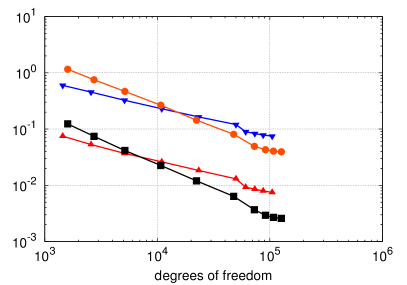
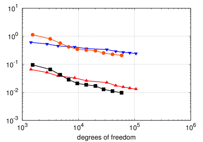
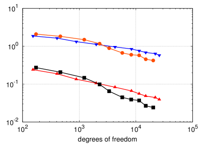
Figure 2: The values of $\mathrm{err}_{u}^{2}$ and $\mathrm{err}_{\chi}$ are displayed in relation to the number of degrees of freedom in a log-log plot for the applications (a) (upper left), (b) (upper right), (c) (lower left) and (d) (lower right). The plotted error estimator values correspond to the discretizations (FE) ($\mathrm{err}_{u}^{2}$ (black line, $\blacksquare$) and $\mathrm{err}_{\chi}$ (brown line, $\bullet$)) and (FE’) ($\mathrm{err}_{u}^{2}$ (red line, $\filledmedtriangleup$) and $\mathrm{err}_{\chi}$ (blue line, $\filledmedtriangledown$)), respectively.

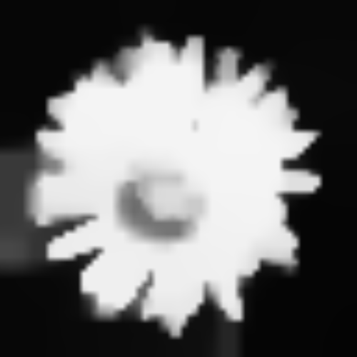
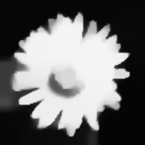
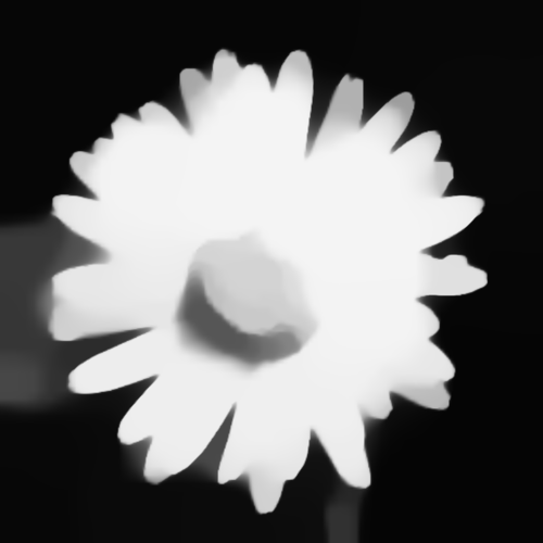
Figure 3: The sequence of solutions $u_{h}$ and a color coding of the corresponding fineness of the adaptive meshes at the $1^{st}$, $2^{nd}$, $3^{rd}$, $4^{th}$ and $5^{th}$ iteration of the adaptive algorithm applied to the input image (c) and computed using the (FE’) discretization.

Table 1 lists (scaled) primal and dual energies, $\mathrm{err}_{u}^{2}$, $\eta_{optimal}$ (the $\eta$ value corresponding to the optimal a posteriori error bound for given $\mathrm{err}^{2}_{u}$), and $\mathrm{err}_{\chi}$ for all input images after the $10$th refinement step of the adaptive algorithm. The value of $\mathrm{err}_{\chi}$ peaks for the application (d) due to the relatively low image resolution.

Figure 2 plots the error estimator $\mathrm{err}_{u}^{2}$ after each refinement step for all input images and both finite element discretizations. In most numerical experiments, the scheme (FE) performs slightly better than the scheme (FE’). For the flower image, the sequence of adaptive meshes and solutions resulting from the adaptive algorithm for the discretization (FE’) is depicted in Figure 3. Figure 4 displays solutions for the discretization (FE’) and the corresponding adaptive meshes together with color coded deciles of $u_{h}$, and the graphs of $\eta\mapsto\mathrm{a}[\mathbf{U}_{h},\eta]$ and $\eta\mapsto\mathrm{err}_{\chi}$. Note that the displayed deciles explicitly indicate the sets $S_{\eta}$ for $\eta=0.1,\,0.2,\,0.3,\,0.4$. Moreover, Figures 5 and 6 show the relaxed solution $u_{h}$ and the thresholded solution $\chi_{h}$ for the remaining discretization schemes and input images.

Figure 4: For images (b) (first and second row) and (c) (last two rows) and the discretization (FE’) the components of the relaxed solution $u_{h}$, $(p_{h})_{1}$, $(p_{h})_{2}$, the resulting solution $\chi_{h}$ are shown after the $10^{th}$ iteration of the adaptive scheme. In the second and fourth row the adaptive grid (after the $6^{th}$ refinement step), deciles of the discrete solution $u_{h}$ encoded with different colors, and the functions $\eta\mapsto\mathrm{a}[\mathbf{U}_{h},\eta]$ (red solid line) and $\eta\mapsto\mathrm{err}_{\chi}$ (blue dashed line) are rendered.

Figure 5: Relaxed solution $u_{h}$, $(p_{h})_{1}$, $(p_{h})_{2}$ for the input image (b) (top row) and (c) (bottom row) using the discretization (FE) (left, after $10$ iterations of the adaptive algorithm) and (FD) (right).

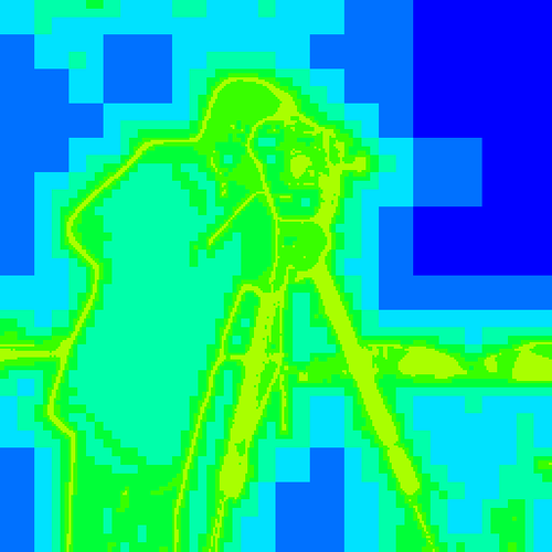
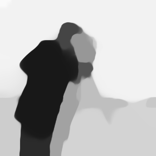
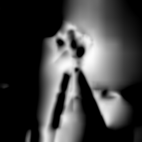
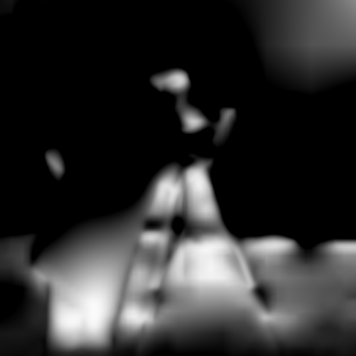
Figure 6: The mesh in the $5^{th}$ and $10^{th}$ iteration, the relaxed solution $u_{h}$, $(p_{h})_{1}$, $(p_{h})_{2}$ and $\chi_{h}$ for the input image (d) using the discretization (FE’) after $10$ iterations of the algorithm.

Finally, we applied the above methods to an analytic function consisting of a weighted sum of two Gaussian kernels. To this end, in each step the functionals and the error estimator are evaluated on the current adaptive grid and not on a prefixed full resolution grid. The results are shown in Figure 7 (with parameters $c_{1}=0.495349$, $c_{2}=0.056845$ and $\nu=5\cdot 10^{-3}$).

Figure 7: First row: Input image $u_{0}$ composed by the superposition of two Gaussian kernels, numerical solutions $u_{h}$, $(p_{h})_{1}$ and $(p_{h})_{2}$ computed via the adaptive algorithm using discretization (FE’). Second row: $\chi_{h}$, deciles and the error estimators in a log-log plot ($\mathrm{err}_{u}^{2}$ in red $\filledmedtriangleup$, $\mathrm{err}_{\chi}$ in blue $\filledmedtriangledown$ for the discretization (FE’) and $\mathrm{err}_{u}^{2}$ in black $\blacksquare$, $\mathrm{err}_{\chi}$ in brown $\bullet$ for the discretization (FE)).

9 Conclusions

We have investigated the a posteriori error estimation for the binary Mumford-Shah model and applied this estimate to two different adaptive finite element discretizations in comparison to a nonadaptive finite difference scheme on a regular grid. The proposed finite element discretizations in combination with the adaptive meshing strategy lead to a substantial reduction of the required degrees of freedom with error values $\mathrm{err}_{u}^{2}$ and $\mathrm{err}_{\chi}$ of about the same magnitude as for a standard finite difference scheme. To improve the resulting estimate of the duality gap $E^{\text{rel}}[v]+{D^{\text{rel}}}[q]$, the finite element schemes (FE) and (FE’) require some oscillation damping smoothing in a post-processing step.

The proposed approach to a posteriori estimates for the binary Mumford-Shah model derived in this paper can be applied straightforwardly to more general problems in computer vision. In fact, the calibration method developed by Alberti, Bouchitté and Dal Maso [1] provides a convex relaxation of non-convex functionals of Mumford-Shah type via the lifting of a variational problem on a $n$-dimensional domain to a minimization problem over characteristic functions of subgraphs in $n+1$ dimensions. In the context of non-convex functionals in vision, this approach was studied by Pock et al. [33, 34]. Applications of such functionals include the computation of minimal partitions [13, 35], the depth map identification from stereo images or the robust extraction of optimal flow fields [34]. Here, an adaptive mesh strategy is expected to have an even larger pay-off due to the increased dimension.

References

- [1] G. Alberti, G. Bouchitté, and G. Dal Maso, The calibration method for the Mumford-Shah functional and free-discontinuity problems, Calc. Var. Partial Differential Equations, 16 (3) (2003), pp. 299–333.
- [2] F. Alter, V. Caselles, and A. Chambolle, A characterization of convex calibrable sets in , Math. Ann., 332 (2005), pp. 329–366.
- [3] L. Ambrosio, Variational problems in SBV and image segmentation, Acta Appl. Math., 17 (1989), pp. 1–40.
- [4] L. Ambrosio, N. Fusco, and D. Pallara, Functions of bounded variation and free discontinuity problems, Oxford Mathematical Monographs, Oxford University Press, New York, 2000.
- [5] L. Ambrosio and V. M. Tortorelli, On the approximation of free discontinuity problems, Bollettino dell’Unione Matematica Italiana, Sezione B, 6 (1992), pp. 105–123.
- [6] S. Bartels, Broken sobolev space iteration for total variation regularized minimization problems. Preprint.
- [7] , Error control and adaptivity for a variational model problem defined on functions of bounded variation, Math. Comp. (online first), (2014).
- [8] B. Berkels, Joint methods in imaging based on diffuse image representations, dissertation, University of Bonn, 2010.
- [9] B. Bourdin and A. Chambolle, Implementation of an adaptive Finite-Element approximation of the Mumford-Shah functional, Numer. Math., 85 (2000), pp. 609–646.
- [10] A. Chambolle, Image segmentation by variatonal methods: Mumford-Shah functional and the discrete approximations, SIAM J. Appl. Math., 55 (1995), pp. 827–863.
- [11] , An algorithm for total variation minimization and applications, Journal of Mathematical Imaging and Vision, 20 (2004), pp. 89–97.
- [12] , Total variation minimization and a class of binary MRF models, in Energy Minimization Methods in Computer Vision and Pattern Recognition, A. Rangarajan et al., eds., vol. 3757 of LNCS, Springer, 2005, pp. 136–152.
- [13] A. Chambolle, D. Cremers, and T. Pock, A convex approach for computing minimal partitions, Tech. Rep. 649, Ecole Polytechnique, Centre de Mathématiques appliquées, UMR CNRS 7641, November 2008.
- [14] , A convex approach to minimal partitions, SIAM Journal on Imaging Sciences, 5 (2012), pp. 1113–1158.
- [15] A. Chambolle and G. Dal Maso, Discrete approximation of the Mumford-Shah functional in dimension two, Mathematical Modelling and Numerical Analysis, 33 (4) (1999), pp. 651–672.
- [16] A. Chambolle and J. Darbon, On total variation minimization and surface evolution using parametric maximum flows, International Journal of Computer Vision, 84 (2009), pp. 288–307.
- [17] A. Chambolle and T. Pock, A first-order primal-dual algorithm for convex problems with applications to imaging, Journal of Mathematical Imaging and Vision, 40 (2011), pp. 120–145.
- [18] T. F. Chan and L. A. Vese, A level set algorithm for minimizing the Mumford-Shah functional in image processing, in IEEE/Computer Society Proceedings of the 1st IEEE Workshop on Variational and Level Set Methods in Computer Vision, 2001, pp. 161–168.
- [19] Y. Chen, T. A. Davis, W. W. Hager, and S. Rajamanickam, Algorithm 887: CHOLMOD, supernodal sparse Cholesky factorization and update/downdate, ACM Transactions on Mathematical Software, 35 (2009), pp. 22:1–22:14.
- [20] D. C. Dobson and C. R. Vogel, Convergence of an iterative method for total variation denoising, SIAM J. Numer. Anal., 34 (1997), pp. 1779–1791.
- [21] I. Ekeland and R. Témam, Convex analysis and variational problems, Society for Industrial and Applied Mathematics, Philadelphia, PA, USA, 1999.
- [22] L. Evans and R. Gariepy, Measure Theory and Fine Properties of Functions, CRC Press, 1992.
- [23] X. Feng and A. Prohl, Analysis of total variation flow and its finite element approximations, M2AN, 37 (2002), pp. 533–556.
- [24] W. Han, A Posteriori Error Analysis Via Duality Theory, vol. 8 of Advances in Mechanics and Mathematics,, Springer, 2005.
- [25] M. Hintermüller and K. Kunisch, Path-following methods for a class of constrained minimization problems in function space, tech. rep., Department of Computational an Applied Mathematics, Rice University, Houston, Texas, July 2004.
- [26] , Total bounded variation regularization as a bilaterally constrained optimization problem, SIAM J. Appl. Math., 64 (2004), pp. 1311–1333.
- [27] S. P. Lloyd, Least squares quantization in PCM, IEEE Transactions on Information Theory, 28 (1982), pp. 129–137.
- [28] L. Modica and S. Mortola, Un esempio di -convergenza, Boll. Un. Mat. Ital. B (5), 14 (1977), pp. 285–299.
- [29] J.-M. Morel and S. Solimini, Variational methods in image segmentation, Progress in Nonlinear Differential Equations and their Applications, 14, Birkhäuser Boston Inc., Boston, MA, 1995.
- [30] D. Mumford and J. Shah, Optimal approximation by piecewise smooth functions and associated variational problems, Communications on Pure and Applied Mathematics, 42 (1989), pp. 577–685.
- [31] M. Nikolova, S. Esedoḡlu, and T. F. Chan, Algorithms for finding global minimizers of image segmentation and denoising models, SIAM Journal on Applied Mathematics, 66 (2006), pp. 1632–1648.
- [32] S. Özışık, B. Riviere, and T. Warburton, On the constants in inverse inequalities in , Tech. Rep. 10-19, Department of Computational & Applied Mathematics, Rice University, 2010.
- [33] T. Pock, D. Cremers, H. Bischof, and A. Chambolle, An algorithm for minimizing the Mumford-Shah functional, in IEEE 12th International Conference on Computer Vision, 2009.
- [34] , Global solutions of variational models with convex regularization, SIAM Journal on Imaging Sciences, 3 (2010), pp. 1122–1145.
- [35] T. Pock, T. Schoenemann, G. Graber, H. Bischof, and D. Cremers, A convex formulation of continuous multi-label problems, in ECCV08, 2008, pp. III: 792–805.
- [36] S. Repin, A posteriori error estimation for variational problems with uniformly convex functionals, Mathematics of Computation, 69 (2000), pp. 481–500.
- [37] , A Posteriori Estimates for Partial Differential Equations, Radon Series on Computational and Applied Mathematics, Wal, 2008.
- [38] R. T. Rockafellar, Convex Analysis, Princeton University Press, 1997.
- [39] L. Rudin, S. Osher, and E. Fatemi, Nonlinear total variation based noise removal algorithms, Physica D, 60 (1992), pp. 259–268.
- [40] J. Shen, -convergence approximation to piecewise constant Mumford-Shah segmentation, in Proceedings of the 7th International Conference on Advanced Concepts for Intelligent Vision Systems (ACIVS 2005), vol. 3708 of Lecture Notes in Computer Science, Springer, 2005, pp. 499–506.
- [41] J. Wang and B. Lucier, Error bounds for finite-difference methods for Rudin-Osher-Fatemi image smoothing, SIAM Journal on Numerical Analysis, 49 (2011), pp. 845–868.