Testing the consistency of the $\omega\pi$ transition form factor with unitarity and analyticity

Abstract

We perform a dispersive analysis of the $\omega\pi$ electromagnetic transition form factor, using as input the discontinuity provided by unitarity below the $\omega\pi$ threshold and including for the first time experimental data on the modulus measured from $e^{+}e^{-}\to\omega\pi^{0}$ at higher energies. The input leads to stringent parameterization-free constraints on the modulus of the form factor below the $\omega\pi$ threshold, which are in disagreement with some experimental values measured from $\omega\to\pi^{0}\gamma^{*}$ decay. We discuss the dependence on the input parameters in the unitarity relation, using for illustration an $N/D$ formalism for the P partial wave of the scattering process $\omega\pi\to\pi\pi$, improved by a simple prescription which simulates the rescattering in the crossed channels. Our results confirm the existence of a conflict between experimental data and theoretical calculations of the $\omega\pi$ form factor in the region around $0.6\,\text{GeV}$ and bring further arguments in support of renewed experimental efforts to measure more precisely the $\omega\to\pi^{0}\gamma^{*}$ decay.

I Introduction

The transition form factors of light mesons play an important role in low energy precision tests of QCD [1]. In particular, they enter as contributions to hadronic light-by-light scattering calculations [2], which are crucial for a more accurate theoretical determination of the standard model prediction for the muon’s anomalous magnetic moment (for recent reviews see [3], [4]).

The case of the $\omega\pi$ electromagnetic form factor is particularly interesting as there are some discrepancies between the theoretical calculations and the experimental data from the decay $\omega\to\pi^{0}\gamma^{*}$ reported in [5, 6, 7]. This form factor was described by Vector Meson Dominance (VMD) model and by a chiral Lagrangian approach in [8, 9]. Calculations based on a standard dispersion relation were performed a long time ago in [10] and recently in [11, 12]. The discontinuity of the form factor required in the Cauchy integral can be expressed in terms of known observables by using unitarity. The two-pion contribution to the unitarity sum gives the discontinuity in terms of the P partial wave of the amplitude of the process $\omega\pi\to\pi\pi$, itself calculated in the dispersion theory [10, 13, 12], and the pion electromagnetic form factor, a quantity which is known with very good precision. However, the two-pion approximation is valid only in a region which extends to a good approximation up to the $\omega\pi$ threshold, $t_{+}=(m_{\omega}+m_{\pi})^{2}$. Due to the lack of information on the discontinuity above this threshold, various assumptions were adopted for the evaluation of the dispersion integral, either by applying the two-pion approximation also at higher energies [10, 11], or by expanding the dispersion integral in powers of a suitable variable [12].

A study performed recently in [14] used as input above the $\omega\pi$ threshold, instead of the discontinuity, a model-independent integral condition on the modulus squared of the $\omega\pi$ form factor. The condition was obtained by using an approach proposed originally by Okubo [15], which has come to be known as the method of unitarity bounds (a recent review of this approach is presented in  [16]). It exploits unitarity and the positivity of the spectral function of a suitable current–current correlator, calculated by operator product expansion (OPE) in the Euclidean region. In the particular case of the $\omega\pi$ form factor, the method, adapted to the specific input conditions available, led eventually to a functional optimization problem of a type considered for the first time in [17, 18]. The solution of the problem yields upper and lower bounds on the modulus of the $\omega\pi$ form factor in the region $4m_{\pi}^{2}\leq t<t_{+}$ [14]. A specific feature of this form factor is that its discontinuity across the cut is not purely imaginary. As a consequence, the form factor is not a real analytic function, as happens in familiar cases like the pion vector form factor. Therefore, in [14] the formalism of bounds was extended to functions which are not real analytic. Although not very stringent, the bounds derived in [14] are in disagreement with the experimental data on the modulus of the form factor in the region around $0.6\,\text{GeV}$, measured from the decay $\omega\to\pi^{0}\gamma^{*}$, confirming thus the conclusion of the analysis [11] based on standard dispersion theory.

It is important to note that the dispersive analyses performed so far did not include experimental data on the form factor available in the scattering region, above the $\omega\pi$ threshold. Measurements of the modulus from the reaction $e^{+}e^{-}\to\omega\pi^{0}$ are reported in [19, 20, 21, 22, 23, 24, 25] (a set of such data is shown in Fig. 1, where we show for completeness also the modulus measured in the decay region $t<t_{-}$, $t_{-}=(m_{\omega}-m_{\pi})^{2}$). In the present paper we consider the problem of including this information in the dispersive formalism. Specifically, we perform an analysis of the form factor using as input the discontinuity for $t<t_{+}$, calculated in a theoretical model based on unitarity, and experimental information on the modulus for $t>t_{+}$. Even though the modulus is not known at all energies, we can implement the information in a conservative way, as a condition on a weighted integral of the modulus squared from $t_{+}$ to infinity. This leads to a mathematical problem similar to that encountered and solved in [14]. The result is expressed in the form of explicit upper and lower bounds on the modulus of the $\omega\pi$ form factor below $t_{+}$, calculable in terms of the discontinuity below $t_{+}$ and the modulus above $t_{+}$. The formalism provides therefore a consistency test for the experimental data on the $\omega\pi$ electromagnetic form factor, which exploits analyticity and unitarity in a parametrization-free way.

The theoretical input of the test consists from the unitarity relation giving the discontinuity of the form factor, which involves the amplitude of the $\pi\omega\to\pi\pi$ scattering. It is of interest to study the influence of the possible uncertainties in this part of the input. The full calculation involves the solution of integral equations known as Khuri-Treiman equations [26]. The amplitudes obtained in this formalism in [13, 12] are available only in numerical form. The older treatment performed in [10], based on $N/D$ formalism, has the advantage of providing explicit expressions. However, it is not entirely satisfactory, as it does not account for the rescatterings between all the final pions in the kinematical region where the decay $\omega\to\pi\pi\pi$ is allowed. It is worthwhile trying to cure the shortcomings of this approach. In this paper we consider an improved $N/D$ treatment, obtained by applying to [10] a prescription proposed in [27] for including finite-width effects in the resonances exchanged in the crossed channels. The improved model captures the essential features of the full solution, still preserving the explicit dependence on the input parameters. This has enabled us to investigate the influence of the uncertainties of the theoretical part of the consistency test.

The paper is organized as follows. In the next section we review the basic definitions and show how the input information on the form factor can be expressed as an extremal problem for analytic functions. In section III we review the main steps of the proof and write down the solution of the extremal problem obtained in Ref. [14]. The results are presented in Sec. IV, where we discuss also their dependence on the parameters of the input. Sec. V contains our conclusions. The paper has an Appendix where we describe briefly the $N/D$ model of [10] and an improved version based on a prescription suggested in [27].

II Input in the consistency test

We begin with a brief description of the form factor and the constraints that it satisfies. We use the conventions of [11], where the form factor $f_{\omega\pi}(t)$ is defined from the matrix element

$$\langle\omega(p_{a},\lambda)\pi^{0}(p_{b})|j_{\mu}(0)|0\rangle=i\epsilon_{\mu\tau\rho\sigma}\epsilon^{\tau*}(p_{a},\lambda)p_{b}^{\rho}q^{\sigma}f_{\omega\pi}(t),$$ (1)

where $j_{\mu}$ is the isovector part of the electromagnetic current, $\lambda$ denotes the $\omega$ polarization, $q=p_{a}+p_{b}$ and $t=q^{2}$. In the convention adopted here the form factor $f_{\omega\pi}(t)$ has dimension of ${\rm GeV}^{-1}$.

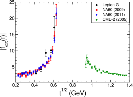
Figure 1: Modulus of the $\omega\pi$ form factor measured from $\omega\to\pi^{0}\gamma^{*}$ decay by Lepton-G [5], NA60 (2009) [6] and NA60 (2011) [7], and from $e^{+}e^{-}\to\omega\pi^{0}$ by CMD-2 (2005) [22].

Unitarity implies that $f_{\omega\pi}(t)$ has a cut along the real axis for $t\geq 4m_{\pi}^{2}$. Keeping the two-pion contribution in the unitarity sum, the discontinuity of $f_{\omega\pi}(t)$ across the cut is written as

$${\rm disc}\,{f_{\omega\pi}(t)}=\frac{iq(t)^{3}}{6\pi\sqrt{t}}F_{\pi}^{*}(t)f_{1}(t)\,\theta\big{(}t-4m_{\pi}^{2}\big{)},\,\,\,t\leq t_{+},$$ (2)

where $q(t)=\sqrt{t/4-m_{\pi}^{2}}$ is the center of mass momentum of the pion pair, $F_{\pi}(t)$ is the pion electromagnetic form factor and $f_{1}(t)$ the P partial-wave amplitude of the scattering

$$\omega(p_{a},\lambda)\,\pi^{0}(p_{b})\to\pi^{+}(q_{1})\,\pi^{-}(q_{2}).$$ (3)

The scattering process is physical for $t\geq t_{+}$. In the region $4m_{\pi}^{2}<t<t_{-}$, where the decay $\omega\to\pi^{+}\pi^{-}\pi^{0}$ is allowed, $f_{1}(t)$ is the P-wave projection of the decay amplitude, while the region $t_{-}<t<t_{+}$ is unphysical.

The amplitude $f_{1}(t)$ was calculated in [10] in the frame of $N/D$ formalism, with the left-hand cut described by poles in the crossed channels due to the exchange of the $\rho$ meson assumed to be stable. In this model, the phase of $f_{1}(t)$ coincides with the $\pi\pi$ P-wave phase shift and exactly compensates in the discontinuity (2) the phase of $F^{*}_{\pi}(t)$, related also to the $\pi\pi$ P wave phase shift $\delta_{1}^{1}$ by Watson theorem [28]. Therefore, the form factor $f_{\omega\pi}(t)$ calculated in [10] is a real analytic function.

In the more complete calculation [13, 11, 12] based on Khuri-Treiman formalism [26], the amplitude $f_{1}(t)$ is obtained by numerically solving a set of integral equations. Due to the rescattering between the final pions in the decay region $4m_{\pi}^{2}<t<t_{-}$, the phase of $f_{1}(t)$ does not coincide with the $\pi\pi$ P-wave phase shift, as one would naively expect from Watson theorem. Therefore, the phases of the two factors in (2) do not compensate each other, and the discontinuity (2) is not purely imaginary [11, 12]. In other words, the $\omega\pi$ form factor is not a real analytic function, which is true also in the case of other transition form factors [27].

The expression (2) is valid only in the region $4m_{\pi}^{2}\leq t<t_{+}$, since above the $\omega\pi$ threshold other intermediate states, besides the two-pion states, contribute in the unitarity sum. So, strictly speaking the discontinuity of $f_{\omega\pi}(t)$ is not available for $t>t_{+}$. On the other hand, the modulus of $f_{\omega\pi}(t)$ can be extracted from experimental data on $e^{+}e^{-}\to\omega\pi^{0}$ process, measured in [19, 20, 21, 22, 23, 24, 25]. The connection between the cross section and the modulus [10, 27] is, in our convention,

$$\sigma_{e^{+}e^{-}\to\omega\pi^{0}}(t)=\frac{4\pi\alpha^{2}}{3}\,\frac{p(t)^{3}}{t^{3/2}}\,|f_{\omega\pi}(t)|^{2}\,,$$ (4)

where $p(t)=\sqrt{(t-t_{-})(t-t_{+})/4t}$ is the center of mass momentum of the $\omega\pi$ pair in the rest system of the virtual photon and we recall that $t_{\pm}=(m_{\omega}\pm m_{\pi})^{2}$.

Using the experimental data on the modulus and the asymptotic behaviour $|f_{\omega\pi}(t)|\sim 1/t$ predicted by perturbative QCD scaling [29], it is possible to obtain a reasonable estimate of a weighted integral over the modulus squared from $t_{+}$ to infinity. Thus, we can write an $L^{2}$-norm condition of the form

$$\frac{1}{\pi}\int_{t_{+}}^{\infty}|f_{\omega\pi}(t)|^{2}\,w(t)\,dt=I,$$ (5)

where $w(t)$ is a suitable weight, chosen such as to allow a precise evaluation of the quantity $I$. We mention that a similar way of including experimental information on the modulus at higher energies was adopted in recent investigations [30, 31] of the pion electromagnetic form factor.

In the present analysis we have considered weights of the simple form

$$w(t)=\frac{1}{t^{c}},$$ (6)

where the value of $c>0$ is taken such as to suppress the high-energy tail of the integral, where the form factor is not known. In practice we evaluated the quantity $I$ using an interpolation of the data on modulus from [22] shown in Fig. 1 from $t_{+}=0.84\,\,\text{GeV}^{2}$ up to $t=1.86\,\,\text{GeV}^{2}$, continued in a smooth way with a modulus $|f_{\omega\pi}(t)|$ decreasing like $1/t$. As will be clear in the next section, for a fixed weight the results of the formalism depend monotonically on the numerical value of $I$, in the sense that a larger $I$ gives weaker results. Therefore, for a conservative estimate, we have used as input in the data region the central values from [22] enlarged by their quoted errors. For $c=2$ this leads to

$$I=4.63\,\,\text{GeV}^{-4},$$ (7)

where the region above $1.86\,\,\text{GeV}^{2}$ contributes to the integral with about 8 %.

Finally, we use as input the value of $|f_{\omega\pi}(0)|$, known experimentally from the $\omega\to\pi^{0}\gamma$ decay rate. The updated value is [32]

$$|f_{\omega\pi}(0)|=(2.30\pm 0.04)\,\text{GeV}^{-1}.$$ (8)

As already mentioned, in the present paper we shall check the consistency of the data shown in Fig. 1 by comparing the data in the decay region with the allowed range of the modulus imposed by unitarity and analyticity. Mathematically, the problem amounts to deriving upper and lower bounds on $|f_{\omega\pi}(t)|$ for $t<t_{+}$, upon the class of functions $f_{\omega\pi}(t)$ analytic in the $t$-plane cut for $t\geq 4m_{\pi}^{2}$, which satisfy the following conditions: (i ) their discontinuity is given by (2) in the region $t<t_{+}$, (ii) they satisfy the constraint (5), and (iii) they satisfy the condition (8). The solution of this mathematical problem will be given in the next section.

III Solution of the extremal problem

An extremal problem of the type mentioned above was solved for the first time in [17, 18] on the class of real analytic functions. The generalization to functions which are not real analytic was investigated in detail in [14]. We do not repeat the whole proof here, but only outline the main steps and write down the solution.

The first step is to map the $t$ plane cut along $t\geq t_{+}$ onto the unit disk $|z|\leq 1$ in the $z\equiv\tilde{z}(t)$ plane. We have adopted the conformal mapping

$$\tilde{z}(t)=\frac{1-\sqrt{1-t/t_{+}}}{1+\sqrt{1-t/t_{+}}},$$ (9)

which brings the origin of the $t$ plane to the origin of the $z$ plane, $\tilde{z}(0)=0$. In the $z$-plane the elastic region $4m_{\pi}^{2}\leq t<t_{+}$ becomes the segment $x_{\pi}\leq x<1$ of the real axis, where $x_{\pi}=\tilde{z}(4m_{\pi}^{2})>0$, and the upper (lower) edges of the cut $t>t_{+}$ become the upper (lower) semicircles.

Further, we construct a so-called outer function [33], i.e. a function analytic and without zeros in $|z|<1$, its modulus on $|z|=1$ being equal to $\sqrt{w(\tilde{t}(z))|d\tilde{t}(z)/dz|}$, where $w(t)$ is the weight appearing in (5) and $\tilde{t}(z)$ is the inverse of the function $\tilde{z}(t)$ defined in (9). The general expression of the outer functions is given in [33] (see also the review [16]). For weights $w(t)$ of the form (6), we obtain for the outer function, denoted as $C(z)$, the exact analytic expression [16]

$$C(z)=(2\sqrt{t_{+}})^{1-c}(1-z)^{1/2}(1+z)^{c-3/2}.$$ (10)

From this expression it follows that $C(x)$ is real and positive for $-1<x<1$, which corresponds in the $t$-plane to the semiaxis $t<t_{+}$.

If we introduce now a new function $h(z)$ by

$$h(z)=C(z)\,f_{\omega\pi}(\tilde{t}(z)),$$ (11)

the condition (5) takes the simple form

$$\frac{1}{2\pi}\int_{0}^{2\pi}d\theta|h(e^{i\theta})|^{2}=I.$$ (12)

The function $h(z)$ is analytic in $|z|<1$ except for a cut along the segment $(x_{\pi},1)$, where its discontinuity is

$${\rm disc}\,h(x)\equiv\Delta(x)=C(x)\,{\rm disc}\,{f_{\omega\pi}(\tilde{t}(x))}.$$ (13)

By expressing $h(z)$ as

$$h(z)=\frac{1}{2\pi i}\int_{x_{\pi}}^{1}\frac{\Delta(x)}{x-z}dx+g(z),$$ (14)

the new function $g(z)$ is analytic in $|z|<1$, as its discontinuity across the cut vanishes:

$${\rm disc}\,{g(x)}=0,\quad\quad x\in(x_{\pi},1).$$ (15)

Since we consider in general form factors that are not real analytic, the function $g(z)$ is analytic, but its values on the real axis may be complex.

We now express the available information on the form factor as a number of constraints on the function $g$. By inserting (14) in (12) we obtain the condition

$$\frac{1}{2\pi}\int_{0}^{2\pi}d\theta\left|\frac{1}{2\pi i}\int_{x_{\pi}}^{1}\frac{\Delta(x)}{x-e^{i\theta}}dx+g(e^{i\theta})\right|^{2}=I,$$ (16)

and using (11) and (14) we write $g(0)$ as

$$g(0)=f_{\omega\pi}(0)C(0)-\frac{1}{2\pi i}\int_{x_{\pi}}^{1}\frac{\Delta(x)}{x}dx.$$ (17)

The problem is to find the maximal allowed range of $|g(z_{1})|$ at an arbitrary given point $z_{1}=\tilde{z}(t_{1})$ in the interval $(x_{\pi},1)$, for functions $g(z)$ analytic in $|z|<1$ and subject both to the boundary condition (16) and the additional constraint (17).

It is useful to denote

$$g(z_{1})=\xi,$$ (18)

where $\xi$ is an unknown parameter. Then one can prove (see for instance [18]) that the allowed range of $\xi$ is described by the inequality

$$\mu_{2}^{2}(\xi)\leq I,$$ (19)

where $\mu_{2}^{2}(\xi)$ is the solution of the functional minimization problem

$$\mu_{2}^{2}(\xi)=\min_{g\in{\cal G}_{\xi}}\frac{1}{2\pi}\int_{0}^{2\pi}d\theta\left|\frac{1}{2\pi i}\int_{x_{\pi}}^{1}\frac{\Delta(x)}{x-e^{i\theta}}dx+g(e^{i\theta})\right|^{2},$$ (20)

upon the class ${\cal G}_{\xi}$ of functions analytic in $|z|<1$, which satisfy the constraint (17) and the additional condition (18) for a given $\xi$.

The constrained minimum norm problem (20) was solved in [14] by the technique of Lagrange multipliers, leading to a solution written in compact form:

$$\mu_{2}^{2}(\xi) =\frac{1}{4\pi^{2}}\int_{x_{\pi}}^{1}\int_{x_{\pi}}^{1}\frac{\Delta(x)\Delta^{*}(y)}{1-xy}dx\,dy+|g(0)|^{2}$$

$$+\frac{1-z_{1}^{2}}{z_{1}^{2}}\,|\xi-g(0)|^{2}.$$ (21)

By inserting (III) in (19) we obtain upper and lower bounds on the parameter $\xi$. Expressed in terms of the form factor $f_{\omega\pi}(t)$ by using Eqs. (11) and (14), they lead to the inequalities [14]:

$$|f_{\omega\pi}(t)| \leq\frac{\left|g(0)+\frac{1}{2\pi i}\int_{x_{\pi}}^{1}\frac{\Delta(x)}{x-\tilde{z}(t)}dx\right|+\frac{\tilde{z}(t)I^{\prime}}{\sqrt{1-\tilde{z}(t)^{2}}}}{C(\tilde{z}(t))}\,,$$

$$|f_{\omega\pi}(t)| \geq\frac{\left|g(0)+\frac{1}{2\pi i}\int_{x_{\pi}}^{1}\frac{\Delta(x)}{x-\tilde{z}(t)}dx\right|-\frac{\tilde{z}(t)I^{\prime}}{\sqrt{1-\tilde{z}(t)^{2}}}}{C(\tilde{z}(t))}\,,$$ (22)

where $\tilde{z}(t)\in(x_{\pi},1)$ is the image of the point $t$ in the $z$-plane, and

$$I^{\prime}=\left[I-\frac{1}{4\pi^{2}}\int_{x_{\pi}}^{1}\int_{x_{\pi}}^{1}\frac{\Delta(x)\Delta^{*}(y)}{1-xy}dx\,dy-|g(0)|^{2}\right]^{1/2}.$$ (23)

We recall that $C(\tilde{z}(t))>0$ for $t<t_{+}$, which justifies its appearance outside the modulus sign in the denominator of (III).

The upper and lower bounds (III) are calculable in terms of the input defined in the previous section. They determine an allowed interval for the modulus $|f_{\omega\pi}(t)|$ at every $t<t_{+}$. From (III) it follows that, for a fixed weigth $w(t)$ in the $L^{2}$-norm constraint (5), the bounds depend monotonically on the value of $I$: smaller values of $I$ lead to narrower allowed intervals for $|f_{\omega\pi}(t)|$ at $t<t_{+}$. We already took into account this property for a conservative estimate of $I$, as discussed in the previous section.

It is useful to remark also that, since the last term in (III) is positive, from (19) and (III) we can write down the inequality

$$\frac{1}{4\pi^{2}}\int_{x_{\pi}}^{1}\int_{x_{\pi}}^{1}\frac{\Delta(x)\Delta^{*}(y)}{1-xy}dx\,dy+|g(0)|^{2}\leq I,$$ (24)

where $g(0)$ is defined in (17) and $\Delta(x)$ is (13). The inequality (24) involves only input quantities and represents a necessary condition that must be satisfied by them. If it is violated, the input is not consistent with analyticity and unitarity.

IV Results

We have investigated several suitable weights of the form (6) and checked that they lead to similar results. The calculations reported below were done with the choice $c=2$, which ensures a good suppression of the high energy part of the integral.

As already mentioned, we have employed the discontinuity (2) of the $\omega\pi$ form factor in the range $(4m_{\pi}^{2},t_{+})$ from the recent dispersive treatment reported in [11] and from the older work [10]. In [11] the pion vector form factor $F_{\pi}(t)$ has been reconstructed from an Omnès representation [34] using as input the pion–pion phase shift $\delta_{1}^{1}(t)$ calculated from Roy equations in [35, 36]. In [10], the pion form factor was described by a Gounaris-Sakurai representation given in Eqs. (39)-(41) of the Appendix. We have checked that the differences between the two representations of the pion form factor are very small and have a negligible influence on the results.

On the other hand, the differences in the partial wave $f_{1}(t)$ used in [10] and [11] are sizable, and have a larger impact on the results. In Fig. 2 we show the allowed bands determined by the upper and lower bounds on the modulus squared (normalized to its value at $t=0$) in the part of the elastic region accessible experimentally in $\omega\to\pi^{0}\mu^{+}\mu^{-}$ decay, calculated using the expressions (III) with input from [10] and [11]. The results shown in Fig. 2 were obtained by varying the input value at $t=0$ inside the error bar given in (8) and taking the weakest bounds, i.e. the largest allowed bands at each energy. For comparison, we also show the result of the dispersive calculation performed in [11], and several experimental data from [5, 6, 7].

Figure 2: Upper and lower bounds compared with experimental data on $|f_{\omega\pi}(t)/f_{\omega\pi}(0)|^{2}$. Cyan band: bounds calculated using in the discontinuity (2) the partial wave amplitude $f_{1}(t)$ from [10]. Grey band: bounds calculated using in the discontinuity (2) the amplitude $f_{1}(t)$ from [11]. The yellow band is the result of the dispersive calculation performed in [11]. The data are from Lepton-G [5], NA60 (2009) [6] and NA60 (2011) [7].

With the input discontinuity from [11], the allowed band is consistent with the dispersion relation calculation performed in that work. The allowed band obtained with the partial wave $f_{1}(t)$ from [10] is shifted upwards and the two bands do not overlap. For both inputs the upper bounds shown in Fig. 2 are significantly lower than the data from [5, 6, 7] in the region around 0.6 GeV.

We mention that the upper and lower bounds shown in Fig. 2 are much more stringent than the upper and lower bounds obtained in [14] with the same input on the discontinuity (2), but with a model-independent condition on the modulus above the $\omega\pi$ threshold.

It is of interest to understand the origin of the difference between the two predictions shown in Fig. 2. To this end, we have calculated the bounds using also the improved version of the $N/D$ model of [10], which includes the effect of rescattering in the crossed channels as discussed in the Appendix. The improvement has the effect of shifting the bounds downwards, towards the band calculated with the input amplitude $f_{1}(t)$ from [13, 11], but the shift is small, of a few percents. For illustration we present in Fig. 3 the bounds calculated with the improved $N/D$ model for $f_{1}(t)$ in the whole range $t<t_{+}$.

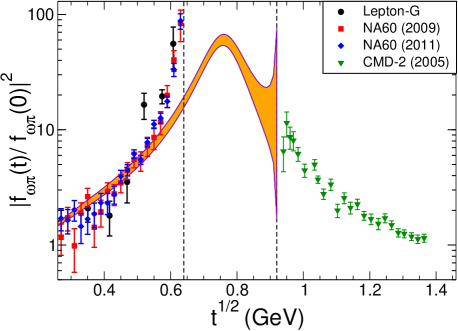
Figure 3: Orange band: bounds on $|f_{\omega\pi}(t)/f_{\omega\pi}(0)|^{2}$ in the whole region $t<t_{+}$, obtained with the improved $N/D$ model. The data are from Lepton-G [5], NA60 (2009) [6], NA60 (2011) [7] and CMD-2 (2005) [22].

Figure 4: Upper and lower bounds on $|f_{\omega\pi}(t)/f_{\omega\pi}(0)|^{2}$ calculated using the improved $N/D$ model, with $g_{\omega\rho\pi}=11.5$ (green band) $g_{\omega\rho\pi}=13.42$ (orange band) and $g_{\omega\rho\pi}=15.5$ (indigo line). The dashed lines are the bounds calculated with the discontinuity (2) from [11]. The red line is the form factor calculated in [8, 9] with a low-energy effective theory.

As follows from Eqs. (30) and (A) of the Appendix, the $N/D$ model contains as input the dimensionless coupling constants $g_{\rho\pi\pi}$ and $g_{\omega\rho\pi}$. The results presented in Figs. 2 and 3 have been obtained using the values from [10]

$$g_{\rho\pi\pi}=5.96,\quad g_{\omega\rho\pi}=13.42.$$ (25)

The quantity $g_{\rho\pi\pi}$ has not changed significantly over the last 40 years, the value (25) being fully consistent with the PDG-2014 width $\Gamma_{\rho}$, quoted below Eq. (41). On the other hand, the coupling $g_{\omega\rho\pi}$ is still not very well known. We note that the dimensionless constant $g_{\omega\rho\pi}$ used here is related to the similar parameter used in [27, 22], which we denote as $\tilde{g}_{\omega\rho\pi}$ to avoid confusion, by $g_{\omega\rho\pi}=m_{\omega}\tilde{g}_{\omega\rho\pi}$. The values $\tilde{g}_{\omega\rho\pi}=(13.8\pm 0.3)\,\,\text{GeV}^{-1}$ obtained in [27] from a global fit of the $\omega\pi$ form factor, and $\tilde{g}_{\omega\rho\pi}=(16.7\pm 0.4\pm 0.6)\,\,\text{GeV}^{-1}$ derived in [22] from a fit of the cross section of $e^{+}e^{-}\to\omega\pi^{0}$, correspond in our notation to the values $g_{\omega\rho\pi}=10.80\pm 0.23$ and $g_{\omega\rho\pi}=13.07\pm 0.31\pm 0.47$, respectively. We note that, while the above references consider parametrizations of the $\omega\pi$ form factor, in the present analysis the coupling $g_{\omega\rho\pi}$ is an input parameter in the model of the amplitude $f_{1}(t)$.

One might ask whether a suitable choice of the parameter $g_{\omega\rho\pi}$ can reduce the conflict between the calculated bounds and the experimental data. We have investigated this question using the improved $N/D$ model discussed in the Appendix. We remark first that for values $g_{\omega\rho\pi}>15.5$ the inequality (24), which expresses a consistency condition on the input, is violated. Therefore, values of $g_{\omega\rho\pi}$ larger than 15.5 are not allowed, being inconsistent with the other input quantites and the general properties of analyticity and unitarity adopted here.

In Fig. 4 we show the allowed bands calculated with three choices of the couplings $g_{\omega\rho\pi}$: the value (25), a smaller value, $g_{\omega\rho\pi}=11.5$, and the maximum allowed value $g_{\omega\rho\pi}=15.5$ mentioned above. In the latter case, when the the inequality (24) is saturated, the quantity $I^{\prime}$ defined in (23) is zero and the upper and lower bounds written in (III) become equal. Therefore, as shown in Fig. 4, the allowed band of the modulus shrinks in this case to a line. The curves show that the bounds exhibit a monotonous dependence on the value of $g_{\omega\rho\pi}$, the band obtained with $g_{\omega\rho\pi}=11.5$ being consistent with the allowed domain obtained using as input $f_{1}(t)$ from the calculation [13, 11]. An important conclusion is that the disagreement with the experimental data around 0.6 GeV is preserved even if the coupling $g_{\omega\rho\pi}$ is increased up to its maximum allowed value.

We show also in Fig. 4 the $\omega\pi$ form factor calculated in [8, 9] within an effective field approach. It exhibits a more rapid increase and slightly exceeds the highest allowed band shown in Fig. 4 near 0.6 GeV.

V Discussion and conclusions

Our study has been motivated by the existence of certain discrepancies between the recent calculations [11, 12, 14] of the $\omega\pi$ electromagnetic transition form factor in the frame of dispersion theory, and the data measured from the $\omega\to\pi^{0}\gamma^{*}$ decay around 0.6 GeV. The present work differs from the previous calculations by the different input used above the $\omega\pi$ threshold $t_{+}$: while the investigations [11, 12] are based on a standard dispersion relation requiring the knowledge of the discontinuity of the form factor along the whole cut, and the work [14] exploits a model-independent integral condition on the modulus, derived from unitarity and perturbative QCD, we have resorted to experimental data obtained from $e^{+}e^{-}\to\omega\pi^{0}$. In order to reduce the bias due to the absence of data at higher energies, we have implemented this information in a conservative way, as a weighted integral (5) of the modulus squared.

The aim of our study was to test the consistency of the experimental and theoretical information available on the $\omega\pi$ form factor in a parametrization-free approach. We have derived upper and lower bounds on the modulus for $t<t_{+}$, using as input the discontinuity (2) in its region of validity below the $\omega\pi$ threshold, and the condition (5) on the modulus above the $\omega\pi$ threshold. Mathematically, the problem is of the type considered some time ago for real-analytic functions in [17, 18] and generalized recently to analytic functions which are not of real type in [14]. Since we used experimental data above $t_{+}$, the results obtained in the present work are much stronger than those obtained in [14], where only a theoretical inequality on the modulus above $t_{+}$ was exploited.

The main theoretical ingredient of the analysis is the partial wave $f_{1}(t)$ entering the discontinuity (2). Therefore, it is of interest to establish the influence of various parameters entering this quantity on the final results. The amplitude $f_{1}(t)$ calculated in [13, 12] is available only in numerical form and is not suitable for this purpose. We have considered therefore the older calculation based on $N/D$ formalism performed in [10], which has the advantage of displaying in an explicit way the dependence on various parameters, and have improved it by a prescription suggested in [27] for including the effect of rescattering in the crossed channels.

Our study has showed that including the rescattering has the effect of shifting down the allowed band for the modulus of the form factor in the region $t<t_{-}$. However, in the frame of the $N/D$ model the effect is quite modest, of a few percents. On the other hand, the bounds are quite sensitive to the coupling $g_{\omega\rho\pi}$, which enters as input in the calculation of $f_{1}(t)$ in the $N/D$ formalism. The results obtained with $f_{1}(t)$ from [13, 11] can be reproduced by using the value $g_{\omega\rho\pi}=11.5$ in the improved $N/D$ formalism. It turns out that values of $g_{\omega\rho\pi}$ larger than 15.5 are excluded, being inconsistent with the remaining elements of the input. By increasing $g_{\omega\rho\pi}$, the allowed bands are pushed upwards. However, as shown in Fig. 4, the narrow band calculated with the maximum allowed value of $g_{\omega\rho\pi}$ is still significantly lower than the experimental data from [5, 6, 7] near 0.6 GeV.

Our results reveal a clear conflict between the experimental data on the modulus of the $\omega\pi$ form factor measured in the decay region $t<t_{-}$ from $\omega\to\pi^{0}\gamma^{*}$ and in the scattering region $t>t_{+}$ from $e^{+}e^{-}\to\omega\pi^{0}$. We note that possible discrepancies between the data on the modulus measured at energies below $t_{-}$ and above $t_{+}$ can be noticed also in the attempts to describe the form factor with specific parametrizations [27]. In contrast, no parametrization of the form factor was necessary in the present analysis. The present work confirms the conclusions of other recent dispersive analyses [11, 14] and brings further arguments in support of renewed experimental efforts to measure more precisely the $\omega$ conversion decays [37, 38].

Acknowledgments

I would like to thank B. Moussallam for very interesting discussions, and B. Ananthanarayan and B. Kubis for a pleasant collaboration on the work [14] and useful suggestions on the manuscript. This work was supported by UEFISCDI under Contract Idei-PCE No 121/2011 and by the Ministry of Education under Contract PN No 09370102/2009.

*

Appendix A Improved $N/D$ treatment of the $\omega\pi\to\pi\pi$ amplitude

The $N/D$ model proposed in [10] does not include the rescattering between all the final pions in the kinematical region where the $\omega$ decay to three pions is allowed. In this Appendix we briefly describe the model and present a simple modification, which is able to capture the characteristic features of the full solution.

For convenience, we use in this Appendix the notation of [10]. The relation with the conventions used in the text is clear by comparing Eqs. (5.1) and (5.3) of [10] with Eqs. (2) and (4) of this paper, respectively. The P partial wave amplitude of the scattering process (3), denoted in [10] as $t^{1}(t)$, has dimensions of $\,\text{GeV}^{-2}$ and is related to the partial wave $f_{1}(t)$ of [13, 11] by

$$t^{1}(t)=\frac{2}{3}\,m_{\omega}\,f_{1}(t).$$ (26)

In the $N/D$ formalism, the amplitude $t^{1}(t)$ is written as [10]

$$t^{1}(t)=t^{1}_{L}(t)+t^{1}_{R}(t),$$ (27)

where $t^{1}_{L}(t)$ has only a left-hand cut and $t^{1}_{R}(t)$ has only a right hand cut for $t>4m_{\pi}^{2}$.

The piece $t^{1}_{L}(t)$ was calculated in [10] as

$$t^{1}_{L}(t)=\frac{1}{2}\int_{-1}^{1}dz\left[d_{00}^{2}(\theta)-d_{00}^{0}(\theta)\right]T_{su}(t,z),$$ (28)

where $z\equiv\cos\theta$, $d_{m^{\prime}m}^{j}(\theta)$ are elements of Wigner’s $d$-matrix and

$$T_{su}(t,z)=-\frac{4}{3}\,g_{1}g_{2}\left(\frac{1}{m_{\rho}^{2}-s(t,z)}+\frac{1}{m_{\rho}^{2}-u(t,z)}\right)$$ (29)

is the $\rho$-pole contribution in the crossed channels. The dimensionless coupling constants are defined as [10]

$$g_{1}\equiv g_{\rho\pi\pi},\quad g_{2}\equiv g_{\omega\rho\pi}$$ (30)

and the Mandelstam variables have the expressions

$$s(t,z)=R(t)+K(t)z,\quad u(t,z)=R(t)-K(t)z,$$ (31)

with

$$R(t)=\frac{m_{\omega}^{2}+3m_{\pi}^{2}-t}{2},\quad K(t)=2q(t)\,p(t),$$ (32)

where $q(t)$ and $p(t)$ are defined below Eqs. (2) and (4), respectively.

The part $t_{R}^{1}(t)$ of the amplitude accounts for the rescattering in the direct channel. In the two-pion approximation, unitarity gives

$${\rm disc}\,[t^{1}(t)\Omega^{-1}(t)]=0,\quad t\geq 4m_{\pi}^{2},$$ (33)

where $\Omega(t)$ is the Omnès function

$$\Omega(t)=\exp\left[\frac{t}{\pi}\int_{4m_{\pi}^{2}}^{\infty}\frac{\delta_{1}^{1}(t^{\prime})}{t^{\prime}(t^{\prime}-t)}\,dt\right],$$ (34)

which is analytic without zeros in the $t$-plane cut for $t>4m_{\pi}^{2}$ and is normalized to $\Omega(0)=1$. It can be written above the cut as

$$\Omega(t+i\epsilon)=|\Omega(t)|e^{i\delta_{1}^{1}(t)},\quad\quad t\geq 4m_{\pi}^{2},$$ (35)

where $\delta_{1}^{1}(t)$ is the phase shift of the P wave of the elastic pion-pion amplitude.

Since $t^{1}_{L}(t)$ is regular for $t\geq 4m_{\pi}^{2}$, from (27) and (35) it follows that

$${\rm disc}\,[t_{R}^{1}(t)\Omega^{-1}(t)]=-2it^{1}_{L}(t){\rm Im}\,\,[\Omega^{-1}(t)].$$ (36)

From the discontinuity one can reconstruct the function by means of a standard dispersion relation, written in [10] as

$$t_{R}^{1}(t)\Omega^{-1}(t)=a+\frac{t-t_{0}}{\pi}\int_{4m_{\pi}^{2}}^{\infty}\frac{t^{1}_{L}(t^{\prime})\sin\delta^{1}_{1}(t^{\prime})}{|\Omega(t^{\prime})|(t^{\prime}-t_{0})(t^{\prime}-t)}dt,$$ (37)

in terms of the unknown subtraction constant $a$. Combined with (27), this leads to

$$t^{1}(t) = \Omega(t)\left[\frac{t^{1}_{L}(t)}{\Omega(t)}+a\right.$$

$$+ \left.\frac{t-t_{0}}{\pi}\int_{4m_{\pi}^{2}}^{\infty}\frac{t^{1}_{L}(t^{\prime})\sin\delta^{1}_{1}(t^{\prime})}{|\Omega(t^{\prime})|(t^{\prime}-t_{0})(t^{\prime}-t)}dt\right]\,.$$

In [10], instead of the Omnès function $\Omega(t)$ a Gounaris-Sakurai parametrization [39] was actually adopted, which is a reasonable approximation on the right hand cut where it is employed. Thus,

$$\Omega(t)\Rightarrow GS(t)=\frac{D(0)}{D(t)},$$ (39)

where $D(t)$ is written as

$$D(t)=m_{\rho}^{2}-t-g(t)-im_{\rho}\Gamma_{\rho}(t).$$ (40)

In this relation

$$\Gamma_{\rho}(t)=\frac{m_{\rho}}{\sqrt{t}}\left(\frac{q(t)}{q(m_{\rho}^{2})}\right)^{3}\,\Gamma_{\rho}$$ (41)

is the energy-dependent $\rho$ width defined in terms of the physical width $\Gamma_{\rho}=147.8\pm 0.9\,\,\text{MeV}$ [32], and

$$g(t)=\frac{m_{\rho}\Gamma_{\rho}}{q(m_{\rho}^{2})}\left(k(t)-k(m_{\rho}^{2})-(t-m_{\rho}^{2})k^{\prime}(m_{\rho}^{2})\right),$$

$$k(t)=\frac{2q(t)^{3}}{\pi\sqrt{t}}\ln\frac{2q(t)+\sqrt{t}}{2m_{\pi}}.$$ (42)

Choosing the subtraction point at $t_{0}=m_{\rho}^{2}$, the behavior of $t^{1}(t)$ near $t=m_{\rho}^{2}$ implies

$$a=\frac{4}{3}\,\frac{g_{1}g_{2}}{D(0)}.$$ (43)

Then, the representation (A) is written finally as [10]

$$t^{1}(t) \!=\! \frac{1}{D(t)}\left[t_{L}^{1}(t)D(t)+\frac{4}{3}\,g_{1}g_{2}\right.$$

$$\!+\! \left.\frac{m_{\rho}(t-m_{\rho}^{2})}{\pi}\int_{4m_{\pi}^{2}}^{\infty}\frac{t^{1}_{L}(t^{\prime})\Gamma_{\rho}(t^{\prime})}{(t^{\prime}-m_{\rho}^{2})(t^{\prime}-t)}dt\right].$$

As follows from (28) and (29), $t_{L}^{1}(t)$ is real for $t>4m_{\pi}^{2}$, which implies that the imaginary terms within the large parantheses compensate each other. Therefore, the phase of $t^{1}(t)$ is equal to the phase of the Omnès function $1/D(t)$, i.e. to the phase shift $\delta^{1}_{1}(t)$. In this model, $t^{1}(t)$ satisfies Watson theorem, and leads to a purely imaginary discontinuity (2) of the $\omega\pi$ form factor. As shown in [13, 11, 12], these properties are no longer valid in the more rigorous treatments of the amplitude.

An obvious shortcoming of the model [10] is the fact that the amplitude $t^{1}_{L}(t)$ was calculated in terms of a $\rho$-meson exchange neglecting the width of the $\rho$. In this approximation the $\omega$ meson is actually stable since its mass is lower that the mass of $\rho\pi$ pair. To improve the model, a straightforward procedure would be to include a finite width for the $\rho$ poles in the denominators of (29). We have adopted the prescription proposed in [27], where finite-width resonance exchange amplitudes with correct analyticity properties were obtained by replacing

$$\frac{1}{m_{\rho}^{2}-s(t,z)}\,\Rightarrow~{}~{}\frac{1}{\pi}\int_{4m_{\pi}^{2}}^{\infty}dx\,\frac{\sigma(x)}{x-s(t,z)},$$ (45)

and similarly for the $u$-channel contribution. The pole was replaced by a modified Breit-Wigner expression which automatically ensures the absence of singularities in the complex plane except for a right-hand cut. As suggested in [27], a reasonable choice for the spectral function $\sigma(x)$ is the imaginary part of the Breit-Wigner propagator:

$$\sigma(x)=\frac{m_{\rho}\Gamma_{\rho}(x)}{(m_{\rho}^{2}-x)^{2}+m_{\rho}^{2}(\Gamma_{\rho}(x))^{2}},$$ (46)

with $\Gamma_{\rho}(x)$ defined in (41). In the limit of zero width, $\Gamma_{\rho}\to 0$, when $\sigma(x)\to\pi\delta(x-m_{\rho}^{2})$, the left side of (45) is recovered.

By inserting the prescription (45) in (28)-(29), the integration upon $z\equiv\cos\theta$ can be performed exactly, leading to

$$t^{1}_{L}(t)=\frac{4g_{1}g_{2}}{3}\,\frac{1}{\pi}\int_{4m_{\pi}^{2}}^{\infty}dx\,\sigma(x)\frac{F(Z)}{K(t)},$$ (47)

where

$$F(y)=\frac{3}{4}\left[2y+(1-y^{2})\ln\frac{y+1}{y-1}\right],$$ (48)

and

$$Z=\frac{x-R(t)}{K(t)},$$ (49)

with $R(t)$ and $K(t)$ defined in (32).

The singularities of $t^{1}_{L}(t)$ in the complex plane arise from the singularities of the function $F(y)$ at $y=\pm 1$ produced by the logarithm, which depend parametrically on $x$. When $x$ varies along the integration range in (47), the singularities describes paths in the complex $t$-plane and in principle can overlap with the $t$-channel unitarity cut along the real semiaxis $t\geq 4m_{\pi}^{2}$. The overlap can be avoided by a suitable prescription. In the present study we have adopted the prescription proposed in [40], which consists in adding to $m_{\omega}^{2}$ a small imaginary part, i.e. $m_{\omega}^{2}\to m_{\omega}^{2}+i\epsilon$, with $\epsilon>0$. With this prescription, we checked numerically that the singularities of $t^{1}_{L}(t)$ do not cross the unitarity cut in the $t$-plane. Moreover, the amplitude $t^{1}_{L}(t)$ has no discontinuity across the line $t\geq 4m_{\pi}^{2}$, although it is no longer real on the unitarity cut.

The points $t=4m_{\pi}^{2}$ and $t=t_{\pm}$, i.e. the physical thresholds and the pseudo-threshold $t_{-}$, require special attention since there the function $K(t)$ defined in (32) vanishes. By using the asymptotic expansion

$$F(y)\sim\frac{1}{y}+\frac{1}{5y^{3}}+\dots,\quad\quad|y|\gg 1,$$ (50)

and the decrease $\sigma(x)\sim 1/x$, we have checked explicitly that in the present model $t^{1}_{L}(t)$ is regular at these points.

Since the amplitude $t^{1}_{L}(t)$ calculated from (47) has no discontinuity across the unitarity cut $t\geq 4m_{\pi}^{2}$, the representation (A) remains valid. However, as mentioned above, $t^{1}_{L}(t)$ is complex for $t\geq 4m_{\pi}^{2}$. Therefore, from (A) it follows that the phase of the amplitude $t^{1}(t)$ for $t\geq 4m_{\pi}^{2}$ is no longer equal to the phase $\delta_{1}^{1}(t)$ of the function $1/D(t)$. Watson theorem, which was valid in the original $N/D$ model, is no longer valid now. Moreover, the amplitude is not an analytic function of real type. These properties are satisfied of course by the exact solution $f_{1}(t)$ calculated in [13, 11, 12].

It is useful to compare the simple improved $N/D$ model presented here with the exact amplitude calculated by solving numerically integral equations of the Khuri-Treiman type. An obvious feature of the $N/D$ model is the lack of symmetry between the direct ($t$) and the crossed ($s$ and $u$) channels. In fact, in the decay region the dynamics in the three two-pion channels must be the same. In the Khuri-Treiman formalism, by iteratively solving the relevant integral equation, the symmetry between the three channels is gradually increased. This adjustment is not performed in the $N/D$ approach, which has a rigid structure. However, by improving the description of the crossed channels in the frame of the $N/D$ model, the main features of the exact partial wave amplitude $f_{1}(t)$, namely the failure of Watson theorem and the breakdown of the reality property, appear in a natural way.

References

- [1] E. Czerwiński et al., arXiv:1207.6556 [hep-ph].
- [2] G. Colangelo, M. Hoferichter, B. Kubis, M. Procura and P. Stoffer, Phys. Lett. B 738, 6 (2014) [arXiv:1408.2517 [hep-ph]].
- [3] F. Jegerlehner and A. Nyffeler, Phys. Rept. 477, 1(2009) [arXiv:0902.3360 [hep-ph]].
- [4] M. Benayoun et al., arXiv:1408.021 [hep-ph].
- [5] R.I. Dzhelyadin et al., Phys. Lett. B 102, 296 (1981) [JETP Lett. 33, 228 (1981)].
- [6] R. Arnaldi et al. [NA60 Collaboration], Phys. Lett. B 677, 260 (2009) [arXiv:0902.2547 [hep-ph]].
- [7] G. Usai [NA60 Collaboration], Nucl. Phys. A 855, 189 (2011).
- [8] C. Terschlüsen and S. Leupold, Phys. Lett. B 691, 191 (2010) [arXiv:1003.1030 [hep-ph]].
- [9] C. Terschlüsen, S. Leupold and M. F. M. Lutz, Eur. Phys. J. A 48, 190 (2012) [arXiv:1204.4125 [hep-ph]].
- [10] G. Köpp, Phys. Rev. D 10, 932 (1974).
- [11] S.P. Schneider, B. Kubis and F. Niecknig, Phys. Rev. D 86, 054013 (2012) [arXiv:1206.3098 [hep-ph]].
- [12] I.V. Danilkin, C. Fernández-Ramírez, P. Guo, V. Mathieu, D. Schott, M. Shi and A.P. Szczepaniak, arXiv: 1409.7708 [hep-ph].
- [13] F. Niecknig, B. Kubis and S. P. Schneider, Eur. Phys. J. C 72 2014 (2012) [arXiv:1203.2501 [hep-ph]].
- [14] B. Ananthanarayan, I. Caprini, B. Kubis, Eur. Phys. J. C 74, 3209 (2014) [arXiv:1410.6276 [hep-ph]].
- [15] S. Okubo, Phys. Rev. D 3, 2807 (1971).
- [16] G. Abbas, B. Ananthanarayan, I. Caprini, I. Sentitemsu Imsong and S. Ramanan, Eur. Phys. J. A 45, 389 (2010) [arXiv:1004.4257 [hep-ph]].
- [17] I. Caprini, J. Phys. A: Math. Gen. 14 1271 (1981).
- [18] I. Caprini, I. Guiasu and E.E. Radescu, Phys. Rev. D 25, 1808 (1982).
- [19] S. I. Dolinsky et al., Phys. Lett. B 174, 453 (1986).
- [20] D. Bisello et al. [DM2 Collaboration], Nucl. Phys. Proc. Suppl. 21, 111 (1991).
- [21] M.N. Achasov et al. [SND Collaboration], Phys. Lett. B 486, 29 (2000) [hep-ex/0005032].
- [22] R.R. Akhmetshin et al. [CMD-2 Collaboration], Phys. Lett. B 562, 173 (2003) [hep-ex/0304009].
- [23] M. N. Achasov et al., JETP Lett. 94, 2 (2012).
- [24] K.W. Edwards et al. [CLEO Collaboration], Phys. Rev. D 61, 072003 (2000) [arXiv:hep-ex/9908024].
- [25] F. Ambrosino et al. [KLOE Collaboration], Phys. Lett. B 669 223 (2008) [arXiv:0808.909 [hep-ex]].
- [26] N.N. Khuri and S.B. Treiman, Phys. Rev. 119, 1115 (1960).
- [27] B. Moussallam, Eur. Phys. J. C 73, 2539 (2013) [arXiv:1305.3143 [hep-ph]].
- [28] K.M. Watson, Phys. Rev. 95, 228 (1954).
- [29] G.P. Lepage and S.J. Brodsky, Phys. Lett. B 87, 359 (1979).
- [30] B. Ananthanarayan, I. Caprini, D. Das and I.S. Imsong, Eur. Phys. J. C 73, 2520 (2013) [arXiv:1302.6373 [hep-ph]].
- [31] B. Ananthanarayan, I. Caprini, D. Das and I.S. Imsong, Phys. Rev. D 89, 036007 (2014) [arXiv:1312.5849 [hep-ph]].
- [32] K.A. Olive et al. [Particle Data Group Collaboration], Chin. Phys. C 38, 090001 (2014).
- [33] P.L. Duren, Theory of Spaces, Academic Press, New York (1970).
- [34] R. Omnès, Nuovo Cim. 8, 316 (1958).
- [35] R. García-Martín, R. Kamiński, J.R. Peláez, J. Ruiz de Elvira and F.J. Ynduráin, Phys. Rev. D 83, 074004 (2011) [arXiv:1102.2183 [hep-ph]].
- [36] I. Caprini, G. Colangelo and H. Leutwyler, Eur. Phys. J. C 72, 1860 (2012) [arXiv:1111.7160 [hep-ph]].
- [37] F.A. Khan [WASA-at-COSY collaboration], in: P. Adlarson et al., arXiv:1204.5509 [nucl-ex].
- [38] M.J. Amaryan [CLAS collaboration], in: K. Kampf et al., arXiv:1308.2575 [hep-ph].
- [39] G.J. Gounaris and J.J. Sakurai, Phys. Rev. Lett. 21, 244 (1968).
- [40] J.B. Bronzan and C. Kacser, Phys. Rev. 132, 2703 (1963).