Equivalence of regression curves

Abstract

This paper investigates the problem whether the difference between two parametric models $m_{1},m_{2}$ describing the relation between a response variable and several covariates in two different groups is practically irrelevant, such that inference can be performed on the basis of the pooled sample. Statistical methodology is developed to test the hypotheses $H_{0}:d(m_{1},m_{2})\geq\varepsilon$ versus $H_{1}:d(m_{1},m_{2})<\varepsilon$ to demonstrate equivalence between the two regression curves $m_{1},m_{2}$ for a pre-specified threshold $\varepsilon$, where $d$ denotes a distance measuring the distance between $m_{1}$ and $m_{2}$. Our approach is based on the asymptotic properties of a suitable estimator $d(\hat{m}_{1},\hat{m}_{2})$ of this distance. In order to improve the approximation of the nominal level for small sample sizes a bootstrap test is developed, which addresses the specific form of the interval hypotheses. In particular, data has to be generated under the null hypothesis, which implicitly defines a manifold for the parameter vector. The results are illustrated by means of a simulation study and a data example. It is demonstrated that the new methods substantially improve currently available approaches with respect to power and approximation of the nominal level.

Keywords and Phrases: dose response studies; nonlinear regression; equivalence of curves; constrained parameter estimation; parametric bootstrap

1 Introduction

Testing statistical hypotheses of equivalence has grown significantly in importance over the last decades, with applications covering such different areas as comparative bioequivalence trials, evaluating negligible trend in animal population growth, and model validation; see, for example, Cade, (2011) and the references therein. Equivalence tests are based on a null hypothesis that a parameter of interest, such as the effect difference of two treatments, is outside an equivalence region defined through an appropriate choice of an equivalence threshold, denoted as $\varepsilon$ in this paper. If the null hypothesis is rejected one can then claim at a pre-specified significance level $\alpha$ that, in the previous example, the two treatments have an equivalent effect [see Wellek, (2010)]. Equivalence testing is often used in regulatory settings because it reverses the burden of proof compared to a standard test of significance.

In this paper, we consider the problem of establishing equivalence of two regression models which are used for the description of the relation between a response variable and several covariates for two different groups, respectively. That is, the objective is to investigate whether the difference between these two models for the two groups is practically irrelevant, so that only one model can be used for both groups based on the pooled sample. Such problems appear for example in population pharmacokinetics (PK) where the goal is to establish bioequivalence of the concentration profiles over time, say $m_{1}$, $m_{2}$, of two compounds. Traditionally, bioequivalence is established by demonstrating equivalence between real valued quantities such as the area under the curve (AUC) or the maximum concentrations ($C_{\max}$) [see Chow and Liu, (1992); Hauschke et al., (2007)]. However, such an approach may be misleading because the two profiles could be very different although they may have similar AUC or $C_{\max}$ values. Hence it might be more reasonable to work directly with the underlying PK profiles instead of the derived summary statistics.

Another application of comparing two dose response curves occurs when assessing the results from one patient population relative to another. For example, the international regulatory guidance document ICH E5, (1997) describes the concept of a bridging study based on, for example, the request of a new geographic region to determine whether data from another region are applicable to its population. If the bridging study shows that dose response, safety and efficacy in the new region are similar to another region, then the study is readily interpreted as capable of bridging the foreign data. As a result, the ability of extrapolating foreign data to a new region depends upon the similarity between the two regions. The ICH E5 guidance does not provide a precise definition of similarity and various concepts have been used in the literature. For example, Tsou et al., (2011) proposed a consistency approach for the assessment of similarity between a bridging study conducted in a new region and studies conducted in the original region. On the other hand, the ICH E5 guidance does require that the safety and efficacy profile in the new region is not substantially different from that in the original region, and similarity can therefore be interpreted as demonstrating “no substantial difference”, which results in an equivalence testing problem [see Liu et al., (2002)].

The problem of establishing equivalence of two regression models while controlling the Type I error rate has found considerable attention in the recent literature. For example, Liu et al., (2009) proposed tests for the hypothesis of equivalence of two regression functions, which are applicable in linear models. Gsteiger et al., (2011) considered non-linear models and suggested a bootstrap method which is based on a confidence band for the difference of the two regression models [see also Liu et al., 2007a ]. Both references use the intersection-union principle [see for example Berger, (1982)] to construct an overall test for equivalence. We demonstrate in this paper that this approach leads to rather conservative test procedures with low power. Instead, we propose to directly estimate the distance, say $d(m_{1},m_{2})$, between the regression curves $m_{1}$ and $m_{2}$ and to decide for the equivalence of the two curves if the estimator is smaller than a given threshold. The critical values of this test can be obtained by asymptotic theory, which describes the limit distribution of an appropriately standardized estimated distance. In order to improve the approximation of the nominal level for small samples sizes a non-standard bootstrap approach is proposed.

In Section 2 we introduce the general problem of demonstrating the equivalence between two regression curves. While the concept of similarity of the two profiles is formulated for a general distance $d$, we concentrate in the subsequent discussion on two specific cases. Section 3 is devoted to the comparison of curves with respect to $L^{2}$-distances. We prove asymptotic normality of the corresponding test statistic and construct an asymptotic level-$\alpha$ test. Moreover, a non-standard bootstrap procedure is introduced, which addresses the particular difficulties arising in the problem of testing (parametric) interval hypotheses. In particular, resampling has to be performed under the null hypothesis $H_{0}:d(m_{1},m_{2})\geq\varepsilon$, which defines (implicitly) a manifold in the parameter space. We prove consistency of the bootstrap test and demonstrate by means of a simulation study that it yields an improvement of the approximation of the nominal level for small sample sizes. In Section 4 the maximal deviation between the two curves is considered as a measure of similarity, for which corresponding results are substantially harder to derive. For example, we prove weak convergence of a corresponding test statistic, but the limit distribution depends in a complicated way on the extremal points of the difference between the “true” curves. This problem is again solved by developing a bootstrap test. The finite sample properties of the new methodology are illustrated in Section 5, where we also provide a comparison with the method of Gsteiger et al., (2011). In particular, it is demonstrated that the methodology proposed in this paper is more powerful than the test proposed by these authors. The methods are illustrated with an example in Section 6. Technical details and proofs are deferred to an appendix in Section 7.

2 Equivalence of regression curves

We consider two, possibly different, regression models $m_{1}$, $m_{2}$ to describe the relationship between a response variable $Y$ and several covariates for two different groups $\ell=1,2$:

$$Y_{\ell,i,j} = m_{\ell}(x_{\ell,i},\beta_{\ell})+\eta_{\ell,i,j}~{},~{}j=1,\ldots,n_{\ell,i},~{}i=1,\ldots,k_{\ell}.$$ (2.1)

Here, the covariate region is denoted by $\mathcal{X}\subset\mathbb{R}^{d}$, $x_{\ell,i}$ denotes the ith dose level (in group $\ell$), $n_{\ell,i}$ the number of patients treated at dose level $x_{\ell,i}$ and $k_{\ell}$ the number of different dose levels in group $\ell$. Further, $n_{\ell}=\sum_{i=1}^{k_{\ell}}n_{\ell,i}$ denotes the sample size in group $\ell$, $n=n_{1}+n_{2}$ the total sample size, and the functions $m_{1}$ and $m_{2}$ in (2.1) define the (non-linear) regression models with $p_{1}$- and $p_{2}$-dimensional parameters $\beta_{1}$ and $\beta_{2}$, respectively. The error terms are assumed to be independent and identically distributed with mean $0$ and variance $\sigma_{\ell}^{2}$ for group $\ell=1,2$. Let $({\cal M},d)$ denote a metric space of real valued functions of the form $g:\mathcal{X}\to\mathbb{R}$ with distance $d$. We assume for all $\beta_{1}$, $\beta_{2}$ that the regression functions satisfy $m_{1}(\cdot,\beta_{1}),m_{2}(\cdot,\beta_{2})\in{\cal M}$, identify the models $m_{\ell}$ by their parameters $\beta_{\ell}$ and denote the distance between the two models by $d(\beta_{1},\beta_{2})(=d(m_{1},m_{2}))$.
We consider the curves $m_{1}$ and $m_{2}$ as equivalent if the distance between the two curves is small, that is $d(\beta_{1},\beta_{2})<\varepsilon$, where $\varepsilon$ is a pre-specified positive constant. In clinical practice, $\varepsilon$ is often denoted as relevance threshold in the sense that if $d(\beta_{1},\beta_{2})<\varepsilon$ the difference between the two curved is believed not to be clinically relevant. In order to establish equivalence of the two dose response curves, we formulate the hypotheses

$$H_{0}:d(\beta_{1},\beta_{2})\geq\varepsilon\quad\mbox{ versus }\quad H_{1}:d(\beta_{1},\beta_{2})<\varepsilon,$$ (2.2)

which in the literature are called precise hypotheses, following Berger and Delampady, (1987). The choice of $\varepsilon$ depends on the particular problem under consideration. For example, when testing for bioequivalence we can conclude that two treatments are not different from one another if the 90% confidence interval of the ratio of a log-transformed exposure measure (AUC and/or $C_{\max}$; see Section 1) falls completely within the range 80-125%, indicating that differences in systemic drug exposure within these limits are not clinically significant [see U.S. Food and Drug Administration, (2003)]. For the comparison of dissolution profiles, which is a special case of the problem considered in this paper, we refer to Appendix I of EMA, (2014) with some recommendations for the choice of the equivalence threshold on the basis of univariate measures [see for example Yuksel et al., (2000)].

In the following we are particularly interested in the metric space of all continuous functions with distances

$$d_{\infty}(\beta_{1},\beta_{2}) = \max_{x\in\mathcal{X}}|m_{1}(x,\beta_{1})-m_{2}(x,\beta_{2})|$$ (2.3)

$$d_{2}(\beta_{1},\beta_{2}) = \int_{\mathcal{X}}|m_{1}(x,\beta_{1})-m_{2}(x,\beta_{2})|^{2}dx.$$ (2.4)

The maximal deviation distance $d_{\infty}$ is of interest, for example, in drug stability studies, where one investigates whether the maximum difference in mean drug content between two batches is no larger than a pre-specified threshold; see, for example, Ruberg and Hsu, (1992) and Liu et al., 2007b . The $L^{2}$-distance $d_{2}$ might be attractive for demonstrating similarity of, for example, two PK models because it measures the squared integral of the difference between the two curves and is therefore related to the areas under the curves, which in turn is often of interest in bioequivalence studies, as mentioned above.
The maximal deviation distance (2.3) has also been considered in Liu et al., (2009) and Gsteiger et al., (2011), who constructed confidence bands for the difference of two regression curves and used the intersection-union principle to derive an overall test for the hypothesis that the two curves are equivalent. In linear models with normally distributed errors this test keeps the significance level not only asymptotically, but exactly at level $\alpha$ for any fixed sample size [see also, Bhargava and Spurrier, (2004) or Liu et al., (2008) for some exact confidence bounds when comparing two linear regression models]. However, the resulting test turns out to be conservative and has low power, as demonstrated in Section 5. This observation can be explained by the fact that the “classical” inversion of a confidence interval for a parameter, say $\mu$, provides a level $\alpha$-test for the hypothesis $H_{0}:\mu=0$, but it yields usually a conservative test for the hypothesis $H_{0}:|\mu|\geq\varepsilon$ [see Wellek, (2010)]. The same phenomenon also appears in the present context of comparing curves. These properties may limit the use of the procedures proposed by Liu et al., (2009) and Gsteiger et al., (2011) in practice, as we would like to maximize the probability of rejecting the null hypothesis if the two regression curves are in fact equivalent as measured by the relevance threshold $\varepsilon$.
In the following, we develop alternatives approaches that are more powerful. Roughly speaking, we consider for $\ell=1,2$ the estimator $m_{\ell}(\cdot,\hat{\beta}_{\ell})$ of the regression curve $m_{\ell}$ and reject the null hypothesis (2.2) for small values of the statistic $\hat{d}=d(\hat{\beta}_{1},\hat{\beta}_{2})$. The critical values can be obtained by asymptotic theory deriving the limit distribution of $\sqrt{n}\ (\hat{d}-d)$ if $n_{1},n_{2}\to\infty$, as developed in the following sections. This approach leads to a satisfactory solution for the $L^{2}$-distance (2.4) based on the quantiles of the normal distribution (see Section 3). However, for the maximal deviation distance (2.3), the limit distribution depends in a complicated way on the extremal points

$$\mathcal{E}=\{x\in\mathcal{X}\mid|\Delta(x,\beta_{1},\beta_{2})|=d_{\infty}(\beta_{1},\beta_{2})\}$$

of the true difference

$$\Delta(x,\beta_{1},\beta_{2})=m_{1}(x,\beta_{1})-m_{2}(x,\beta_{2}).$$ (2.5)

Moreover, in small sample trials the approximation of the nominal level of a given test based on asymptotic theory may not be valid. In order to obtain a more accurate approximation of the nominal level, we propose a non-standard bootstrap procedure and prove its consistency. This procedure has to be constructed in a way such that it addresses the particular features of the equivalence hypotheses (2.2). In particular, data have to be generated under the null hypothesis $d(\beta_{1},\beta_{2})\geq\varepsilon$, which implicitly defines a manifold for the vector of parameters $(\beta^{T}_{1},\beta^{T}_{2})^{T}\in\mathbb{R}^{p_{1}+p_{2}}$ of both models. The non-differentiability of the maximal deviation distance $d_{\infty}$ exhibits some technical difficulties of such an approach, and for this reason we begin the discussion with the $L^{2}$-distance $d_{2}$.

3 Comparing curves by $L^{2}$-distances

In this section we construct a test for the equivalence of the two regression curves with respect to the squared $L^{2}-$distance, i.e. we consider hypotheses of the form

$$H_{0}:\int_{\mathcal{X}}(m_{1}(x,\beta_{1})-m_{2}(x,\beta_{2}))^{2}dx\geq\varepsilon_{2}\mbox{~{}~{}versus~{}~{}}H_{1}:\int_{\mathcal{X}}(m_{1}(x,\beta_{1})-m_{2}(x,\beta_{2}))^{2}dx<\varepsilon_{2}.$$ (3.1)

Note that under certain regularity assumptions (see the Appendix for details) the ordinary least squares (OLS) estimators, say $\hat{\beta}_{1}$ and $\hat{\beta}_{2}$, of the parameters ${\beta_{1}}$ and ${\beta_{2}}$ can usually be linearized in the form

$$\sqrt{n_{\ell}}\ (\hat{\beta}_{\ell}-\beta_{\ell})=\frac{1}{\sqrt{n_{\ell}}}\sum^{k_{\ell}}_{i=1}\sum^{n_{\ell,i}}_{j=1}\phi_{\ell,i,j}+o_{\mathbb{P}}(1),\qquad\ell=1,2,$$ (3.2)

where the functions $\phi_{\ell,i,j}$ are given by

$$\phi_{\ell,i,j}=\tfrac{\eta_{\ell,i,j}}{\sigma^{2}_{\ell}}\Sigma^{-1}_{\ell}\tfrac{\partial}{\partial b_{\ell}}m_{\ell}(x_{\ell,i,},b_{\ell})\big{|}_{b_{\ell}=\beta_{\ell}},\qquad\ell=1,2,$$ (3.3)

and the $(p_{\ell}\times p_{\ell})-$dimensional matrices $\Sigma_{\ell}$ are defined by

$$\Sigma_{\ell}={1\over\sigma_{\ell}^{2}}\sum_{i=1}^{k_{\ell}}\zeta_{\ell,i}\tfrac{\partial}{\partial b_{\ell}}m_{\ell}(x_{\ell,i,},b_{\ell})\big{|}_{b_{\ell}=\beta_{\ell}}\big{(}\tfrac{\partial}{\partial b_{\ell}}m_{\ell}(x_{\ell,i,},b_{\ell})\big{|}_{b_{\ell}=\beta_{\ell}}\big{)}^{T}~{},~{}~{}\ell=1,2.$$ (3.4)

For these arguments we assume that the matrices $\Sigma_{\ell}$ are non-singular and that the sample sizes $n_{\ell}$ converge to infinity such that

$$\lim_{n_{\ell}\to\infty}{n_{\ell,i}\over n_{\ell}}=\zeta_{\ell,i}>0~{},~{}~{}i=1,\ldots,k_{\ell}~{},~{}\ell=1,2,$$ (3.5)

and

$$\lim_{n_{1},n_{2}\rightarrow\infty}\frac{n}{n_{1}}=\lambda\in(1,\infty).$$ (3.6)

It then follows by straightforward calculation that the OLS estimators are asymptotically normal distributed, i.e.

$$\sqrt{n_{\ell}}(\hat{\beta}_{\ell}-\beta_{\ell})\stackrel{{\scriptstyle\mathcal{D}}}{{\rightarrow}}\mathcal{N}(0,\Sigma_{\ell}^{-1})~{},~{}\ell=1,2,$$ (3.7)

where the symbol $\stackrel{{\scriptstyle\cal D}}{{\longrightarrow}}$ means weak convergence (convergence in distribution for real valued random variables). The asymptotic variance in (3.7) can easily be estimated by replacing the parameters $\beta_{\ell}$, $\sigma_{\ell}$ and $\zeta_{\ell,i}$ in (3.4) by their estimators $\hat{\beta}_{\ell}$, $\hat{\sigma}_{\ell}$ and $n_{\ell,i}/n_{\ell}\ (\ell=1,2)$. The resulting estimator will be denoted by $\hat{\Sigma}_{\ell}$ throughout this paper. The null hypothesis in (3.1) is then rejected whenever

$$\hat{d}_{2}:=d_{2}(\hat{\beta}_{1},\hat{\beta}_{2})=\int_{\mathcal{X}}(m_{1}(x,\hat{\beta_{1}})-m_{2}(x,\hat{\beta_{2}}))^{2}dx<c,$$ (3.8)

where $c$ denotes a pre-specified constant defined through the level of the test. In order to determine this constant we will derive the asymptotic distribution of the statistic $\hat{d}_{2}$. The following result is proved in the Appendix.

Theorem 3.1.

If Assumptions 7.1 - 7.5 from the Appendix, (3.5) and (3.6) are satisfied, we have

$$\sqrt{n}{(\hat{d}_{2}-d_{2})}\stackrel{{\scriptstyle\mathcal{D}}}{{\longrightarrow}}\mathcal{N}(0,{\sigma_{d_{2}}^{2}}),$$ (3.9)

where the asymptotic variance is given by

$$\sigma_{d_{2}}^{2}=\sigma^{2}_{d_{2}}(\beta_{1},\beta_{2})=4{\int_{\mathcal{X}\times\mathcal{X}}\Delta(x,\beta_{1},\beta_{2})\Delta(y,\beta_{1},\beta_{2})k(x,y)dxdy},$$ (3.10)

$\Delta(x,\beta_{1},\beta_{2})$ is defined in (2.5) and the kernel $k(x,y)$ is given by

$$k(x,y) := \lambda\big{(}\tfrac{\partial}{\partial b_{1}}m_{1}(x,b_{1})\big{|}_{b_{1}=\beta_{1}}\big{)}^{T}\Sigma_{1}^{-1}\tfrac{\partial}{\partial b_{1}}m_{1}(y,b_{1})\big{|}_{b_{1}=\beta_{1}}$$ (3.11)

$$+ \tfrac{\lambda}{\lambda-1}\big{(}\tfrac{\partial}{\partial b_{2}}m_{2}(x,b_{2})\big{|}_{b_{2}=\beta_{2}}\big{)}^{T}\Sigma_{2}^{-1}\tfrac{\partial}{\partial b_{2}}m_{2}(y,b_{2})\big{|}_{b_{2}=\beta_{2}}.$$

Theorem 3.1 provides a simple asymptotic level-$\alpha$ test for the hypothesis (3.1) of equivalence of two regression curves. More precisely, if $\hat{\sigma}_{d_{2}}^{2}=\sigma^{2}_{d_{2}}(\hat{\beta}_{1},\hat{\beta}_{2})$ denotes the (canonical) estimator of the asymptotic variance in (3.10), then the null hypothesis in (3.1) is rejected if

$$\hat{d}_{2}<\varepsilon_{2}+\frac{\hat{\sigma}_{d_{2}}}{\sqrt{n}}u_{\alpha},$$ (3.12)

where $u_{\alpha}$ denotes the $\alpha$-quantile of the standard normal distribution. Note that by the nature of the problem the quantile of this test depends on the threshold $\varepsilon_{2}$. The finite sample properties of this test will be investigated in Section 5.1.

Remark 3.2.

It follows from Theorem 3.1 that the test (3.12) has asymptotic level $\alpha$ and is consistent if $n_{1},n_{2}\to\infty$. More precisely, if $\Phi$ denotes the cumulative distribution function of the standard normal distribution, we have for the probability of rejecting the null hypothesis in (3.1)

$$\mathbb{P}\Big{(}\hat{d}_{2}<\varepsilon_{2}+\frac{\hat{\sigma}_{d_{2}}}{\sqrt{n}}u_{\alpha}\Big{)} = \mathbb{P}\Big{(}\frac{\sqrt{n}}{\hat{\sigma}_{d_{2}}}(\hat{d}_{2}-d_{2})<\frac{\sqrt{n}}{\hat{\sigma}_{d_{2}}}(\varepsilon_{2}-d_{2})+u_{\alpha}\Big{)}~{}.$$

Under continuity assumptions it follows that $\hat{\sigma}^{2}_{d_{2}}\stackrel{{\scriptstyle\mathbb{P}}}{{\longrightarrow}}\sigma^{2}_{d_{2}}$ and Theorem 3.1 yields $\sqrt{n}\ (\hat{d}_{2}-d_{2})/\hat{\sigma}_{d_{2}}\stackrel{{\scriptstyle\cal D}}{{\longrightarrow}}\mathcal{N}(0,1)$. This gives

$$\mathbb{P}\Big{(}\hat{d}_{2}\leq\varepsilon_{2}+\frac{\hat{\sigma}_{d_{2}}}{\sqrt{n}}u_{\alpha}\Big{)}\stackrel{{\scriptstyle\longrightarrow}}{{\scriptstyle{n_{1},n_{2}\to\infty}}}\left\{\begin{array}[]{ccc}0&\mbox{if}&d_{2}>\varepsilon_{2}\\ \alpha&\mbox{if}&d_{2}=\varepsilon_{2}\\ 1&\mbox{if}&d_{2}<\varepsilon_{2}\\ \end{array}\right.\qquad.$$

The test (3.12) can be recommended if the sample sizes are reasonable large. However, we will demonstrate in Section 5 that for very small sample sizes, the critical values provided by this asymptotic theory may not provide an accurate approximation of the nominal level, and for this reason we will also investigate a parametric bootstrap procedure to generate critical values for the statistic $\hat{d}_{2}$.

Algorithm 3.3.

(parametric bootstrap for testing precise hypotheses)

• Calculate the OLS-estimators $\hat{\beta_{1}}$ and $\hat{\beta_{2}}$, the corresponding variance estimators

  $$\hat{\sigma}^{2}_{\ell}=\frac{1}{n_{\ell}}\sum^{k_{\ell}}_{i=1}\sum^{n_{\ell,i}}_{j=1}(Y_{\ell,i,j}-m_{\ell}(x_{\ell,i},\hat{\beta}_{\ell}))^{2};\qquad\ell=1,2,$$

  and the test statistic $\hat{d}_{2}=d_{2}(\hat{\beta}_{1},\hat{\beta}_{2})$ defined by (3.8).

• Define estimators of the parameters $\beta_{1}$ and $\beta_{2}$ by

  $${\hat{\hat{\beta}}_{\ell}}=\left\{\begin{array}[]{ccc}\hat{\beta}_{\ell}&\mbox{if}&\hat{d}_{2}\geq\varepsilon_{2}\\ \tilde{\beta}_{\ell}&\mbox{if}&\hat{d}_{2}<\varepsilon_{2}\end{array}\right.\quad\ell=1,2,$$ (3.14)

  where $\tilde{\beta}_{1},\tilde{\beta}_{2}$ denote the OLS-estimators of the parameters $\beta_{1},\beta_{2}$ under the constraint

  $$d_{2}(\beta_{1},\beta_{2})=\int_{\mathcal{X}}(m_{1}(x,\beta_{1})-m_{2}(x,\beta_{2}))^{2}dx=\varepsilon_{2}.$$ (3.15)

  Finally, define ${\hat{\hat{d}}_{2}}=d_{2}({\hat{\hat{\beta}}_{1}},{\hat{\hat{\beta}}_{2}})$ and note that ${\hat{\hat{d}}_{2}}\geq\varepsilon_{2}$.

• Bootstrap test

  • Generate bootstrap data under the null hypothesis, that is

    $$Y_{\ell,i,j}^{*}=m_{\ell}(x_{\ell,i},\hat{\hat{\beta_{\ell}}})+\eta_{\ell,i,j}^{*}~{},i=1,\ldots,n_{\ell,i},~{}\ell=1,2,$$ (3.16)

    where the errors $\eta^{*}_{\ell,i,j}$ are independent normally distributed such that $\eta_{\ell,i,j}^{*}\sim\mathcal{N}(0,\hat{\sigma}_{\ell}^{2})$.

  • Calculate the OLS estimators $\hat{\beta}^{*}_{1}$ and $\hat{\beta}^{*}_{2}$ and the test statistic

    $$\hat{d}^{*}_{2}=d_{2}(\hat{\beta}^{*}_{1},\hat{\beta}^{*}_{2})=\int_{\mathcal{X}}(m_{1}(x,\hat{\beta}^{*}_{1})-m_{2}(x,\hat{\beta}_{2}^{*}))^{2}dx$$

    from the bootstrap data. Denote by $\hat{q}_{\alpha,2}$ the $\alpha-$quantile of the distribution of the statistic $\hat{d}^{*}_{2}$, which depends on the data $\left\{Y_{l,i,j}|l=1,2;\ j=1,...n_{l,i};\ i=1,...,k_{l}\right\}$ through the estimators $\hat{\hat{\beta}}_{1}$ and $\hat{\hat{\beta}}_{2}$.

  The steps (i) and (ii) are repeated $B$ times to generate replicates $\hat{d}^{*}_{2,1},\dots,\hat{d}^{*}_{2,B}$ of $\hat{d}^{*}_{2}$. If $\hat{d}^{*(1)}_{2}\leq\ldots\leq\hat{d}^{*(B)}_{2}$ denotes the corresponding order statistic, the estimator of the quantile of the distribution of $\hat{d}^{*}_{2}$ is defined by $\hat{q}_{\alpha,2}^{(B)}:=\hat{d}_{2}^{*(\lfloor B\alpha\rfloor)}$, and the null hypothesis is rejected if

  $$\hat{d}_{2}<\hat{q}_{\alpha,2}^{(B)}.$$ (3.17)

  Note that the bootstrap quantile $\hat{q}_{\alpha,2}^{(B)}$ depends on the threshold $\varepsilon_{2}$ which is used in the hypothesis (3.1), but we do not reflect this dependence in our notation.

The following result shows that the bootstrap test (3.17) has asymptotic level $\alpha$ and is consistent if $n_{1},n_{2}\to\infty$. Its proof can be found in the Appendix.

Theorem 3.4.

Assume that the conditions of Theorem 3.1 are satisfied.

• If the null hypothesis in $\eqref{hypothesesL2}$ holds, then we have for any $\alpha\in(0,0.5)$

  $$\lim_{n_{1},n_{2}\rightarrow\infty}\mathbb{P}(\hat{d}_{2}<\hat{q}_{\alpha,2})=\left\{\begin{array}[]{ccc}0&\mbox{if}&d_{2}>\varepsilon_{2}\\ \alpha&\mbox{if}&d_{2}=\varepsilon_{2}\end{array}.\right.$$ (3.18)

• If the alternative in $\eqref{hypothesesL2}$ holds, then we have for any $\alpha\in(0,0.5)$

  $$\lim_{n_{1},n_{2}\rightarrow\infty}\mathbb{P}(\hat{d}_{2}<\hat{q}_{\alpha,2})=1.$$ (3.19)

4 Comparing curves by their maximal deviation

In this section we construct a test for the equivalence of the two regression curves with respect to the maximal absolute deviation (2.3). The corresponding test statistic is given by the maximal deviation distance

$$\hat{d}_{\infty}=d_{\infty}(\hat{\beta}_{1},\hat{\beta}_{2})=\max_{x\in\mathcal{X}}|m_{1}(x,\hat{\beta}_{1})-m_{2}(x,\hat{\beta}_{2})|$$ (4.1)

between the two estimated regression functions, where $\hat{\beta}_{1},\hat{\beta}_{2}$ are the OLS-estimators from the two samples. In order to describe the asymptotic distribution of the statistic $\hat{d}_{\infty}$ we define the set of extremal points

$$\mathcal{E}=\big{\{}x\in\mathcal{X}\big{|}\ |m_{1}(x,\beta_{1})-m_{2}(x,\beta_{2})|=d_{\infty}\big{\}}$$ (4.2)

and introduce the decomposition $\mathcal{E}=\mathcal{E}^{+}\cup\mathcal{E}^{-}$, where

$$\mathcal{E}^{\mp}=\big{\{}x\in\mathcal{X}\big{|}\ m_{1}(x,\beta_{1})-m_{2}(x,\beta_{2})=\mp\ d_{\infty}\big{\}}.$$ (4.3)

The following result is proved in the Appendix.

Theorem 4.1.

If $d_{\infty}>0$ and the assumptions of Theorem 3.1 are satisfied, then

$$\sqrt{n}\ (\hat{d}_{\infty}-d_{\infty})\stackrel{{\scriptstyle\cal D}}{{\longrightarrow}}\mathcal{Z}:=\max\big{\{}\max_{x\in\mathcal{E}^{+}}G(x),\max_{x\in\mathcal{E}^{-}}(-G(x))\big{\}},$$ (4.4)

where $\{G(x)\}_{x\in\mathcal{X}}$ denotes a Gaussian process defined by

$$G(x)=\big{(}\tfrac{\partial}{\partial b_{1}}m_{1}(x,b_{1})\big{|}_{b_{1}=\beta_{1}}\big{)}^{T}\sqrt{\lambda}\Sigma_{1}^{-1/2}Z_{1}-\big{(}\tfrac{\partial}{\partial b_{2}}m_{2}(x,b_{2})\big{|}_{b_{2}=\beta_{2}}\big{)}^{T}\sqrt{\tfrac{\lambda}{\lambda-1}}\Sigma_{2}^{-1/2}Z_{2},$$ (4.5)

and $Z_{1}$ and $Z_{2}$ are independent $p_{1}$- and $p_{2}$-dimensional standard normal distributed random variables, respectively, i.e. $Z_{\ell}\sim{\cal N}(0,I_{p_{\ell}})$, $\ell=1,2$.

In principle, Theorem 4.1 provides an asymptotic level $\alpha$-test for the hypotheses

$$H_{0}:d_{\infty}(\beta_{1},\beta_{2})\geq\varepsilon_{\infty}\quad\mbox{versus}\quad H_{1}:d_{\infty}(\beta_{1},\beta_{2})<\varepsilon_{\infty}$$ (4.6)

by rejecting the null hypotheses whenever $\hat{d}_{\infty}<q_{\alpha,\infty}$, where $q_{\alpha,\infty}$ denotes the $\alpha$-quantile of the distribution of the random variable $\mathcal{Z}$ defined in (4.4). However, this distribution has a very complicated structure. For example, if $\mathcal{E}=\{x_{0}\}$ the distribution of $\mathcal{Z}$ is a centered normal distribution but with variance

$$\sigma_{\infty}^{2} = \lambda\big{(}\tfrac{\partial}{\partial b_{1}}m_{1}(x_{0},b_{1})\big{|}_{b_{1}=\beta_{1}}\big{)}^{T}\Sigma_{1}^{-1}\tfrac{\partial}{\partial b_{1}}m_{1}(x_{0},b_{1})\big{|}_{b_{1}=\beta_{1}}$$ (4.7)

$$+ \tfrac{\lambda}{\lambda-1}\big{(}\tfrac{\partial}{\partial b_{2}}m_{2}(x_{0},b_{2})\big{|}_{b_{2}=\beta_{2}}\big{)}^{T}\Sigma_{2}^{-1}\tfrac{\partial}{\partial b_{2}}m_{2}(x_{0},b_{2})\big{|}_{b_{2}=\beta_{2}}$$

which depends on the location of the (unique) extremal point $x_{0}$. In general (more precisely in the case $\#\mathcal{E}>1$) the distribution of $\mathcal{Z}$ is the distribution of a maximum of dependent Gaussian random variables, where the variances and the dependence structure depend on the location of the extremal points of the function $\Delta(\cdot,\beta_{1},\beta_{2})$. Because the estimation of these points is very difficult, we propose a bootstrap approach to obtain suitable quantiles. The bootstrap test is defined in the same way as described in Algorithm 3.3, where the distance $d_{2}$ is replaced by the maximal deviation $d_{\infty}$. The corresponding quantile obtained in Step 3(ii) of Algorithm 3.3 is now denoted by $\hat{q}_{\alpha,\infty}^{(B)}$, while the theoretical quantile of the bootstrap distribution is denoted by $\hat{q}_{\alpha,\infty}$. The following result is proved in the Appendix and shows that the test, which rejects the null hypothesis in (4.6) whenever

$$\hat{d}_{\infty}<\hat{q}_{\alpha,\infty}^{(B)},$$ (4.8)

has asymptotic level $\alpha$ and is consistent. Interestingly the quality of the approximation of the nominal level of the test depends on the cardinality of the set $\mathcal{E}$.

Theorem 4.2.

Suppose that the assumptions of Theorem 4.1 hold.

• If the null hypothesis in $\eqref{h0inf}$ is satisfied and the set $\mathcal{E}$ defined in (4.2) consists of one point, then we have for any $\alpha\in(0,0.5)$

  $$\lim_{n_{1},n_{2}\rightarrow\infty}\mathbb{P}\big{(}\hat{d}_{\infty}<\hat{q}_{\alpha,\infty}\big{)}=\left\{\begin{array}[]{ccc}0&\mbox{if}&d_{\infty}>\varepsilon_{\infty}\\ \alpha&\mbox{if}&d_{\infty}=\varepsilon_{\infty}.\end{array}\right.$$ (4.9)

• Let $F_{\mathcal{Z}}$ denote the distribution function of the random variable $\mathcal{Z}$ defined in (4.4) and $q_{\mathcal{Z},\alpha}$ its $\alpha$-quantile. Assume that $F_{\mathcal{Z}}$ is continuous at $q_{\mathcal{Z},\alpha}$ and $q_{\mathcal{Z},\alpha}<0$. If the null hypothesis in $\eqref{h0inf}$ is satisfied we have

  $$\limsup_{n_{1},n_{2}\rightarrow\infty}\mathbb{P}\big{(}\hat{d}_{\infty}<\hat{q}_{\alpha,\infty}\big{)}\leq\alpha.$$ (4.10)

• If the alternative in $\eqref{h0inf}$ is satisfied, then we have for any $\alpha\in(0,0.5)$

  $$\lim_{n_{1},n_{2}\rightarrow\infty}\mathbb{P}\big{(}\hat{d}_{\infty}<\hat{q}_{\alpha,\infty}\big{)}=1.$$ (4.11)

Remark 4.3.

(a) The condition in part (2) of Theorem 4.2 is a non-trivial assumption. By results in Tsirel’son, (1976), the distribution of $\mathcal{Z}$ has at most one jump at the left boundary of its support and is continuous to the right of that. The condition on $F_{\mathcal{Z}}$ to be continuous at $q_{\mathcal{Z},\alpha}$ is thus equivalent to requiring that the mass at the left endpoint of the support of $F_{\mathcal{Z}}$ is smaller than $\alpha$. In some cases it is possible to show that $F_{\mathcal{Z}}$ is continuous on $\mathbb{R}$, i.e. the mass at its left support point is zero. For example, this follows from Theorem 3 of Chernozhukov et al., (2015) provided that the condition

$$\inf_{x\in\mathcal{E}}\Big{(}\|\tfrac{\partial}{\partial b_{1}}m_{1}(x,b_{1})\big{|}_{b_{1}=\beta_{1}}\|+\|\tfrac{\partial}{\partial b_{2}}m_{2}(x,b_{2})\big{|}_{b_{2}=\beta_{2}}\|\Big{)}>0$$ (4.12)

holds.
The assumption (4.12) is always fulfilled if one of the models contains an additive (placebo) effect because in this case the first entry of the gradient $\tfrac{\partial}{\partial b_{\ell}}m_{\ell}(x,b_{\ell})\big{|}_{b_{\ell}=\beta_{\ell}}$ equals $1$. Furthermore, if the two models are of the form $m_{\ell}(x,\beta_{\ell})=\beta_{\ell,1}\cdot m_{\ell}^{0}(x,\beta_{\ell}^{0})$ for $l=1,2$ with $\beta_{\ell}=(\beta_{\ell,1},\beta_{\ell}^{0})$ (for example Michalis-Menten models), we have

$$\tfrac{\partial}{\partial b_{\ell}}m_{\ell}(x,b_{\ell})\big{|}_{b_{\ell}=\beta_{\ell}}=\big{(}m_{\ell}^{0}(x,\beta_{\ell}^{0}),\tfrac{\partial}{\partial b_{\ell}^{0}}m_{\ell}^{0}(x,b_{\ell}^{0})\big{|}_{b_{\ell}^{0}=\beta_{\ell}^{0}}\big{)},\ \ell=1,2.$$

Consequently, if (4.12) was not fulfilled, there would exist $x_{0}\in\mathcal{E}$ such that $m_{\ell}^{0}(x_{0},\beta_{\ell}^{0})=0,\ \ell=1,2$, and as $x_{0}\in\mathcal{E}$ it holds

$$d_{\infty}=\left|m_{1}(x_{0},\beta_{1})-m_{2}(x_{0},\beta_{2})\right|=\left|\beta_{1,1}\cdot m_{1}^{0}(x_{0},\beta_{1}^{0})-\beta_{2,1}\cdot m_{2}^{0}(x_{0},\beta_{2}^{0})\right|=0$$

This yields $m_{1}\equiv m_{2}$ and does not correspond to the null hypothesis.
(c) Note that the asymptotic Type I error rate of the bootstrap test is precisely $\alpha$ at the boundary of the hypothesis (i.e. $d_{\infty}=\varepsilon_{\infty}$) if the cardinality of $\mathcal{E}$ is one. On the other hand, if the set $\mathcal{E}$ contains more than one point, part (2) of Theorem 4.2 indicates that the corresponding bootstrap test is usually conservative, even at the boundary of the hypothesis. These results are confirmed by a simulation study in Section 5.2.

5 Finite sample properties

In this section we investigate the finite sample properties of the asymptotic and bootstrap tests proposed in Sections 3 and 4 in terms of power and size. For the distance $d_{\infty}$ we also provide a comparison with the approach from Gsteiger et al., (2011). Their method follows from (3.5) - (3.7) and an application of the Delta method [see for example Van der Vaart, (1998)] so that the prediction $m_{1}(x,\hat{\beta}_{1})-m_{2}(x,\hat{\beta}_{2})$ for the difference of the two regression models at the point $x$ is approximately normally distributed. That is,

$$\frac{m_{1}(x,\hat{\beta}_{1})-m_{2}(x,\hat{\beta}_{2})-(m_{1}(x,\beta_{1})-m_{2}(x,\beta_{2}))}{\hat{\tau}_{n_{1},n_{2}}(x,\hat{\beta}_{1},\hat{\beta}_{2})}\stackrel{{\scriptstyle\mathcal{D}}}{{\longrightarrow}}\mathcal{N}(0,1),$$

where

$$\hat{\tau}^{2}_{n_{1},n_{2}}(x,\hat{\beta}_{1},\hat{\beta}_{2})=\sum_{\ell=1}^{2}\tfrac{1}{n_{\ell}}\big{(}\tfrac{\partial}{\partial\beta_{\ell}}m_{\ell}(x,\ \beta_{\ell})\big{|}_{\beta_{\ell}=\hat{\beta}_{\ell}}\big{)}^{T}\hat{\Sigma}_{\ell}^{-1}\tfrac{\partial}{\partial\beta_{\ell}}m_{\ell}(x,\beta_{\ell})\big{|}_{\beta_{\ell}=\hat{\beta}_{\ell}}$$ (5.1)

and $\hat{\Sigma}_{\ell}$ denotes the estimator of the variance in (3.4), which is obtained by replacing the parameters $\sigma_{\ell}$, $\beta_{\ell}$ and $\zeta_{\ell,i}$ by their estimators $\hat{\sigma}_{\ell}$, $\hat{\beta}_{\ell}$, and $n_{\ell,i}/n_{\ell}\ (\ell=1,2)$. Gsteiger et al., (2011) proposed a test based on the pointwise confidence bands derived by Liu et al., 2007a , that is

$$m_{1}(x,\hat{\beta}_{1})-m_{2}(x,\hat{\beta}_{2})\pm\ z_{1-\alpha}\hat{\tau}_{n_{1},n_{2}}(x,\hat{\beta}_{1},\hat{\beta}_{2}),$$

where $z_{1-\alpha}$ denotes the $(1-\alpha)$-quantile of the standard normal distribution. A test for the hypotheses (4.6) is finally obtained by rejecting the null hypothesis and conclude for equivalence, if the maximum (minimum) of the upper (lower) confidence band is smaller (larger) than $\varepsilon_{\infty}$ ($-\varepsilon_{\infty}$). A particular advantage of this test is that it directly refers to the distance (2.3), which has a nice interpretation in many applications. Moreover, in linear models (with normally distributed errors) it is an exact level-$\alpha$ test. However, the resulting test is conservative and has low power compared to the methods proposed in this paper as shown in Section 5.2.

All results in this and the following section are based on $1000$ simulation runs and the quantiles of the bootstrap tests have been obtained by $B=300$ bootstrap replications. In all examples the dose range is given by the interval ${\cal X}=[0,4]$ and an equal number of patients is allocated at the five dose levels $x_{\ell,1}=0,x_{\ell,2}=1$, $x_{\ell,3}=2$, $x_{\ell,4}=3$, $x_{\ell,5}=4$ in both groups (that is $k_{1}=k_{2}=5$).

5.1 Tests based on the distance $d_{2}$

For the sake of brevity we restrict ourselves to a comparison of two shifted EMAX-models

$$m_{1}(x,\beta_{1})=\beta_{11}+\frac{\beta_{12}x}{\beta_{13}+x}\qquad\mbox{and}\qquad m_{2}(x,\beta_{2})=\beta_{21}+\frac{\beta_{22}x}{\beta_{23}+x},$$ (5.2)

where $\beta_{1}=(\beta_{11},\beta_{12},\beta_{13})=(\delta,5,1)$ and $\beta_{2}=(\beta_{21},\beta_{22},\beta_{23})=(0,5,1)$. In Tables 1 and 2 we display the simulated Type I error rates of the bootstrap test (3.17) and the asymptotic test (3.12) for $\varepsilon_{2}=1$ in (3.1) and various configurations of $\sigma^{2}_{1}$, $\sigma^{2}_{2}$, $n_{1}$, $n_{2}$ and $\delta$. In the interior of the null hypothesis (i.e. $d_{2}>\varepsilon_{2}$) the Type I error rates of the tests (3.12) and (3.17) are smaller than the nominal level as predicted by Remark 3.2. For both tests we observe a rather precise approximation of the nominal level (even for small sample sizes) at the boundary of the null hypothesis (i.e. $d_{2}=1$). In some cases the approximation of the nominal level by the bootstrap test (3.17) is slightly more accurate and for this reason we recommend to use the bootstrap test (3.17) to establish equivalence of two regression models with respect to the $L^{2}$-distance.

			$\alpha=0.05$			$\alpha=0.1$
			$(\sigma_{1}^{2},\sigma_{2}^{2})$			$(\sigma_{1}^{2},\sigma_{2}^{2})$
$(n_{1},n_{2})$	$\delta$	$d_{2}$	$(0.25,0.25)$	$(0.5,0.5)$	$(0.25,0.5)$	$(0.25,0.25)$	$(0.5,0.5)$	$(0.25,0.5)$
$(10,10)$	1	4	0.000	0.000	0.000	0.000	0.000	0.000
$(10,10)$	0.75	2.25	0.004	0.002	0.001	0.000	0.002	0.000
$(10,10)$	0.5	1	0.051	0.064	0.052	0.101	0.120	0.118
$(10,20)$	1	4	0.000	0.000	0.000	0.000	0.000	0.000
$(10,20)$	0.75	2.25	0.000	0.000	0.000	0.000	0.000	0.000
$(10,20)$	0.5	1	0.055	0.060	0.051	0.104	0.111	0.101
$(20,20)$	1	4	0.000	0.000	0.000	0.000	0.000	0.000
$(20,20)$	0.75	2.25	0.001	0.002	0.000	0.004	0.005	0.001
$(20,20)$	0.5	1	0.057	0.058	0.050	0.125	0.107	0.097
$(50,50)$	1	4	0.000	0.000	0.000	0.000	0.000	0.000
$(50,50)$	0.75	2.25	0.001	0.000	0.000	0.002	0.000	0.000
$(50,50)$	0.5	1	0.057	0.048	0.054	0.097	0.114	0.093

Table 1: Simulated Type I error rates of the bootstrap test (3.17) for the equivalence of two shifted EMAX models defined in (5.2). The threshold in (3.1) is chosen as $\varepsilon_{2}=1$.

			$\alpha=0.05$			$\alpha=0.1$
			$(\sigma_{1}^{2},\sigma_{2}^{2})$			$(\sigma_{1}^{2},\sigma_{2}^{2})$
$(n_{1},n_{2})$	$\delta$	$d_{2}$	$(0.25,0.25)$	$(0.5,0.5)$	$(0.25,0.5)$	$(0.25,0.25)$	$(0.5,0.5)$	$(0.25,0.5)$
$(10,10)$	1	4	0.002	0.002	0.002	0.000	0.002	0.003
$(10,10)$	0.75	2.25	0.005	0.005	0.009	0.007	0.011	0.016
$(10,10)$	0.5	1	0.080	0.042	0.049	0.102	0.061	0.071
$(10,20)$	1	4	0.000	0.000	0.000	0.000	0.000	0.000
$(10,20)$	0.75	2.25	0.007	0.012	0.007	0.017	0.015	0.012
$(10,20)$	0.5	1	0.055	0.063	0.060	0.081	0.078	0.084
$(20,20)$	1	4	0.000	0.000	0.000	0.000	0.000	0.000
$(20,20)$	0.75	2.25	0.000	0.001	0.002	0.017	0.003	0.006
$(20,20)$	0.5	1	0.060	0.066	0.080	0.090	0.091	0.096
$(50,50)$	1	4	0.000	0.000	0.000	0.000	0.000	0.000
$(50,50)$	0.75	2.25	0.000	0.000	0.000	0.000	0.000	0.001
$(50,50)$	0.5	1	0.041	0.058	0.052	0.071	0.087	0.073

Table 2: Simulated Type I error rates of the asymptotic test (3.12) for the equivalence of two shifted EMAX models defined in (5.2). The threshold in (3.1) is chosen as $\varepsilon_{2}=1$

In Tables 3 and 4 we display the power of the two tests under various alternatives specified by the value $\beta_{1,1}=\delta$ in model (5.2). We observe a reasonable power of both tests in all cases under consideration. In those cases where the asymptotic test (3.12) keeps (or exceeds) its nominal level it is slightly more powerful than the bootstrap test (3.17). The opposite performance can be observed in those cases where the asymptotic test is conservative (e.g., if $\alpha=10\%,\ n_{1}=n_{2}=10$). We also note that the power of both tests is a decreasing function of the distance $d_{2}$, as predicted by the asymptotic theory.

			$\alpha=0.05$			$\alpha=0.1$
			$(\sigma_{1}^{2},\sigma_{2}^{2})$			$(\sigma_{1}^{2},\sigma_{2}^{2})$
$(n_{1},n_{2})$	$\delta$	$d_{2}$	$(0.25,0.25)$	$(0.5,0.5)$	$(0.25,0.5)$	$(0.25,0.25)$	$(0.5,0.5)$	$(0.25,0.5)$
$(10,10)$	0.25	0.25	0.210	0.118	0.134	0.300	0.212	0.256
$(10,10)$	0.1	0.04	0.294	0.132	0.186	0.427	0.250	0.312
$(10,10)$	0	0	0.351	0.145	0.176	0.467	0.286	0.340
$(10,20)$	0.25	0.25	0.257	0.125	0.191	0.392	0.234	0.305
$(10,20)$	0.1	0.04	0.395	0.164	0.254	0.535	0.305	0.395
$(10,20)$	0	0	0.437	0.158	0.291	0.598	0.290	0.474
$(20,20)$	0.25	0.25	0.392	0.171	0.225	0.534	0.302	0.382
$(20,20)$	0.1	0.04	0.560	0.308	0.418	0.720	0.460	0.562
$(20,20)$	0	0	0.610	0.314	0.390	0.757	0.462	0.555
$(50,50)$	0.25	0.25	0.724	0.460	0.554	0.825	0.595	0.825
$(50,50)$	0.1	0.04	0.961	0.691	0.821	0.982	0.824	0.973
$(50,50)$	0	0	0.984	0.734	0.865	0.998	0.861	0.999

Table 3: Simulated power of the bootstrap test (3.17) for the equivalence of two shifted EMAX models defined in (5.2). The threshold in (3.1) is chosen as $\varepsilon_{2}=1.$

			$\alpha=0.05$			$\alpha=0.1$
			$(\sigma_{1}^{2},\sigma_{2}^{2})$			$(\sigma_{1}^{2},\sigma_{2}^{2})$
$(n_{1},n_{2})$	$\delta$	$d_{2}$	$(0.25,0.25)$	$(0.5,0.5)$	$(0.25,0.5)$	$(0.25,0.25)$	$(0.5,0.5)$	$(0.25,0.5)$
$(10,10)$	0.25	0.25	0.264	0.103	0.175	0.311	0.131	0.217
$(10,10)$	0.1	0.04	0.351	0.139	0.196	0.431	0.183	0.247
$(10,10)$	0	0	0.381	0.120	0.222	0.468	0.168	0.279
$(10,20)$	0.25	0.25	0.305	0.147	0.256	0.382	0.192	0.317
$(10,20)$	0.1	0.04	0.468	0.218	0.359	0.536	0.268	0.438
$(10,20)$	0	0	0.510	0.220	0.358	0.570	0.272	0.455
$(20,20)$	0.25	0.25	0.423	0.271	0.321	0.493	0.328	0.341
$(20,20)$	0.1	0.04	0.640	0.328	0.501	0.716	0.407	0.585
$(20,20)$	0	0	0.690	0.351	0.501	0.781	0.438	0.573
$(50,50)$	0.25	0.25	0.659	0.475	0.534	0.740	0.562	0.649
$(50,50)$	0.1	0.04	0.965	0.750	0.868	0.974	0.813	0.911
$(50,50)$	0	0	0.980	0.848	0.937	0.991	0.893	0.946

Table 4: Simulated power of the asymptotic test (3.12) for the equivalence of two shifted EMAX models defined in (5.2). The threshold in (3.1) is chosen as $\varepsilon_{2}=1$.

5.2 Tests based on the distance $d_{\infty}$

We now investigate the maximum deviation distance and also provide a comparison with the test proposed by Gsteiger et al., (2011). Motivated by the discussion in Section 4 we distinguish the cases where the cardinality of the set $\mathcal{E}$ is one or larger than one. The results will show that with an increasing size of the set $\mathcal{E}$ the test is getting more conservative.

Example 5.1.

($\#\mathcal{E}=1$) We begin with a comparison of an EMAX with an exponential model, that is

$$m_{1}(x,\beta_{1})=\beta_{11}+\frac{\beta_{12}x}{\beta_{13}+x}\qquad\mbox{and}\qquad m_{2}(x,\beta_{2})=\beta_{21}+\beta_{22}\cdot(\exp{(\tfrac{x}{\beta_{23}})}-1),$$ (5.3)

where $\beta_{1}=(\beta_{11},\beta_{12},\beta_{13})=(1,2,1)$ and $\beta_{2}=(\beta_{21},\beta_{22},\beta_{23})=(\delta,2.2,8)$ [see Figure 1].

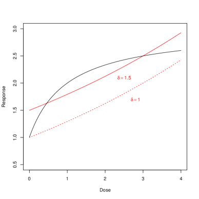
Figure 1: The models defined in (5.3) for two different choices of $\delta$.

In Table 5 we display the simulated rejection probabilities of the bootstrap test (4.8) under the null hypothesis in (4.6), where $\varepsilon_{\infty}=1$.
If the cardinality of the set $\mathcal{E}$ is one, the distribution of the test statistic $\hat{d}_{\infty}$ is a centered normal distribution with variance defined in (4.7). Thus, if the unique extremal point has been estimated, we obtain an estimate, say $\hat{\sigma}_{\infty}^{2},$ of the asymptotic variance of the statistic $\hat{d}_{\infty}$. The null hypothesis is now rejected (at asymptotic level $\alpha$), whenever

$$\hat{d}_{\infty}<\varepsilon_{\infty}+{\hat{\sigma}_{\infty}\over\sqrt{n}}u_{\alpha}~{},$$ (5.4)

where $u_{\alpha}$ is the $\alpha-$quantile of the standard normal distribution. The results for this test are given in Table 6. We observe that the bootstrap test (4.8) keeps its nominal level at the boundary of the null hypothesis, whereas the level is smaller in the interior (this confirms the theoretical results from Section 4). The approximation is less precise for small sample sizes. Compared to the bootstrap test based on the distance $d_{2}$ the test (4.8) is conservative. The asymptotic test (5.4) is very conservative, even for relative large sample sizes (see Table 6). A possible explanation for this observation consists in the fact that the estimation of the extremal point is a difficult problem. In Table 5 we also display the rejection probabilities of the test of Gsteiger et al., (2011) in brackets. This test is very conservative as its level is practically $0$ for almost all cases under consideration.
The simulated power of the bootstrap and the asymptotic $d_{\infty}$-test is displayed in Table 7 and 8. We observe a substantially better performance of the bootstrap test (4.8) in all cases of consideration. In Table 7 we also display the rejection probabilities of the test of Gsteiger et al., (2011) in brackets and we conclude that the methods proposed in this paper yield a substantial improvement for small sample sizes or large variances.

			$\alpha=0.05$			$\alpha=0.1$
			$(\sigma_{1}^{2},\sigma_{2}^{2})$			$(\sigma_{1}^{2},\sigma_{2}^{2})$
$(n_{1},n_{2})$	$\delta$	$d_{\infty}$	$(0.25,0.25)$	$(0.5,0.5)$	$(0.25,0.5)$	$(0.25,0.25)$	$(0.5,0.5)$	$(0.25,0.5)$
$(10,10)$	0.25	1.5	0.001 (0.000)	0.001 (0.000)	0.000 (0.000)	0.000 (0.000)	0.004 (0.000)	0.000 (0.000)
$(10,10)$	0.5	1.25	0.005 (0.000)	0.011 (0.000)	0.006 (0.000)	0.013 (0.000)	0.030 (0.000)	0.020 (0.000)
$(10,10)$	0.75	1	0.045 (0.007)	0.037 (0.000)	0.036 (0.001)	0.102 (0.021)	0.086 (0.002)	0.090 (0.007)
$(10,20)$	0.25	1.5	0.000 (0.000)	0.002 (0.000)	0.000 (0.000)	0.000 (0.000)	0.002 (0.000)	0.000 (0.000)
$(10,20)$	0.5	1.25	0.004 (0.000)	0.013 (0.000)	0.005 (0.000)	0.015 (0.000)	0.025 (0.000)	0.009 (0.000)
$(10,20)$	0.75	1	0.045 (0.017)	0.046 (0.002)	0.028 (0.004)	0.099 (0.042)	0.104 (0.011)	0.079 (0.017)
$(20,20)$	0.25	1.5	0.000 (0.000)	0.000 (0.000)	0.000 (0.000)	0.000 (0.000)	0.000 (0.000)	0.000 (0.000)
$(20,20)$	0.5	1.25	0.001 (0.000)	0.004 (0.000)	0.000 (0.000)	0.006 (0.000)	0.018 (0.000)	0.011 (0.000)
$(20,20)$	0.75	1	0.034 (0.013)	0.038 (0.003)	0.048 (0.007)	0.091 (0.033)	0.100 (0.020)	0.104 (0.026)
$(50,50)$	0.25	1.5	0.000 (0.000)	0.000 (0.000)	0.000 (0.000)	0.000 (0.000)	0.000 (0.000)	0.000 (0.000)
$(50,50)$	0.5	1.25	0.000 (0.000)	0.000 (0.000)	0.000 (0.000)	0.002 (0.000)	0.001 (0.000)	0.000 (0.000)
$(50,50)$	0.75	1	0.051 (0.013)	0.059 (0.009)	0.058 (0.010)	0.096 (0.040)	0.108 (0.043)	0.105 (0.096)

Table 5: Simulated Type I error rates of the bootstrap test (4.8) for the equivalence of an EMAX and an exponential model defined by (5.3). The threshold in (4.6) is chosen as $\varepsilon_{\infty}=1$. The numbers in brackets show the simulated Type I error rates of the test proposed in Gsteiger et al., (2011).

			$\alpha=0.05$			$\alpha=0.1$
			$(\sigma_{1}^{2},\sigma_{2}^{2})$			$(\sigma_{1}^{2},\sigma_{2}^{2})$
$(n_{1},n_{2})$	$\delta$	$d_{\infty}$	$(0.25,0.25)$	$(0.5,0.5)$	$(0.25,0.5)$	$(0.25,0.25)$	$(0.5,0.5)$	$(0.25,0.5)$
$(10,10)$	0.25	1.5	0.000	0.000	0.000	0.000	0.000	0.000
$(10,10)$	0.5	1.25	0.001	0.001	0.000	0.003	0.004	0.001
$(10,10)$	0.75	1	0.012	0.005	0.003	0.029	0.010	0.001
$(10,20)$	0.25	1.5	0.000	0.000	0.000	0.000	0.000	0.000
$(10,20)$	0.5	1.25	0.000	0.005	0.001	0.000	0.007	0.003
$(10,20)$	0.75	1	0.019	0.006	0.009	0.038	0.014	0.023
$(20,20)$	0.25	1.5	0.000	0.000	0.000	0.000	0.000	0.000
$(20,20)$	0.5	1.25	0.000	0.000	0.001	0.000	0.001	0.001
$(20,20)$	0.75	1	0.011	0.036	0.009	0.033	0.025	0.027
$(50,50)$	0.25	1.5	0.000	0.000	0.000	0.000	0.000	0.000
$(50,50)$	0.5	1.25	0.000	0.000	0.000	0.000	0.003	0.000
$(50,50)$	0.75	1	0.016	0.015	0.012	0.039	0.039	0.041

Table 6: Simulated Type I error rates of the asymptotic test (5.4) for the equivalence of an EMAX and an exponential model defined by (5.3). The threshold in (4.6) is chosen as $\varepsilon_{\infty}=1$

			$\alpha=0.05$			$\alpha=0.1$
			$(\sigma_{1}^{2},\sigma_{2}^{2})$			$(\sigma_{1}^{2},\sigma_{2}^{2})$
$(n_{1},n_{2})$	$\delta$	$d_{\infty}$	$(0.25,0.25)$	$(0.5,0.5)$	$(0.25,0.5)$	$(0.25,0.25)$	$(0.5,0.5)$	$(0.25,0.5)$
$(10,10)$	1	0.75	0.160 (0.026)	0.093 (0.004)	0.125 (0.007)	0.297 (0.083)	0.225 (0.007)	0.229 (0.033)
$(10,10)$	1.5	0.5	0.237 (0.037)	0.133 (0.003)	0.164 (0.009)	0.383 (0.117)	0.231 (0.018)	0.309 (0.029)
$(10,20)$	1	0.75	0.185 (0.084)	0.123 (0.006)	0.159 (0.025)	0.320 (0.162)	0.226 (0.035)	0.283 (0.089)
$(10,20)$	1.5	0.5	0.300 (0.087)	0.175 (0.005)	0.269 (0.035)	0.457 (0.190)	0.305 (0.043)	0.414 (0.120)
$(20,20)$	1	0.75	0.214 (0.130)	0.138 (0.022)	0.171 (0.054)	0.393 (0.248)	0.271 (0.086)	0.345 (0.137)
$(20,20)$	1.5	0.5	0.401 (0.190)	0.229 (0.036)	0.363 (0.080)	0.604 (0.356)	0.398 (0.122)	0.523 (0.189)
$(50,50)$	1	0.75	0.504 (0.400)	0.274 (0.183)	0.363 (0.297)	0.662 (0.552)	0.416 (0.326)	0.532 (0.433)
$(50,50)$	1.5	0.5	0.777 (0.667)	0.491 (0.294)	0.606 (0.493)	0.877 (0.791)	0.648 (0.478)	0.739 (0.604)

Table 7: Simulated power of the bootstrap test (4.8) for the equivalence of an EMAX and an exponential model defined by (5.3). The threshold in (4.6) is chosen as $\varepsilon_{\infty}=1$. The numbers in brackets show the simulated power of the test proposed in Gsteiger et al., (2011).

			$\alpha=0.05$			$\alpha=0.1$
			$(\sigma_{1}^{2},\sigma_{2}^{2})$			$(\sigma_{1}^{2},\sigma_{2}^{2})$
$(n_{1},n_{2})$	$\delta$	$d_{\infty}$	$(0.25,0.25)$	$(0.5,0.5)$	$(0.25,0.5)$	$(0.25,0.25)$	$(0.5,0.5)$	$(0.25,0.5)$
$(10,10)$	1	0.75	0.042	0.006	0.011	0.109	0.017	0.046
$(10,10)$	1.5	0.5	0.064	0.008	0.014	0.140	0.026	0.047
$(10,20)$	1	0.75	0.114	0.014	0.048	0.199	0.047	0.106
$(10,20)$	1.5	0.5	0.129	0.018	0.059	0.228	0.052	0.127
$(20,20)$	1	0.75	0.151	0.036	0.064	0.285	0.093	0.170
$(20,20)$	1.5	0.5	0.209	0.060	0.104	0.360	0.120	0.202
$(50,50)$	1	0.75	0.417	0.206	0.303	0.569	0.337	0.440
$(50,50)$	1.5	0.5	0.706	0.267	0.408	0.826	0.462	0.630

Table 8: Simulated power of the asymptotic test (5.4) for the equivalence of an EMAX and an exponential model defined by (5.3). The threshold in (4.6) is chosen as $\varepsilon_{\infty}=1$.

In the remaining part of this section we consider three further scenarios, where the true maximum absolute distance of the models $m_{1}$ and $m_{2}$ is attained at more than one point. In this case, an asymptotic test based on the maximum deviation is not available and therefore only the bootstrap test can be used. Our results demonstrate that the test is conservative compared to the scenario before, where $\#\mathcal{E}=1$. This confirms our theoretical findings in Theorem 4.2. Moreover, the test gets more conservative if the size of the set $\mathcal{E}$ increases. We also display (the numbers in brackets) the corresponding values for the test of Gsteiger et al., (2011), which is very conservative and less powerful than the bootstrap test in all cases under consideration.

Example 5.2.

($\#\mathcal{E}=2$) We consider two EMAX models, given by

$$m_{1}(x,\beta_{1})=\beta_{11}+\frac{\beta_{12}x}{\beta_{13}+x}\text{ and }m_{2}(x,\beta_{2})=\beta_{21}+\frac{\beta_{22}x}{\beta_{23}+x},$$ (5.5)

where $\beta_{1}=(\beta_{11},\beta_{12},\beta_{13})=(\delta,6,2)$ and $\beta_{2}=(\beta_{21},\beta_{22},\beta_{23})=(0,5,1)$. In this case the maximum absolute difference of $d_{\infty}=\delta$ is attained at the boundary points of the design space, that is $\mathcal{E}=\{0,4\}$. The corresponding rejection probabilities under the null hypothesis are presented in Table 9. We observe that the bootstrap test keeps its level in all situations, but it is conservative (see also Theorem 4.2). The test of Gsteiger et al., (2011) is even more conservative. We also observe an improvement in power by the new test in comparison with the test of Gsteiger et al., (2011), in particular for small samples sizes (see Table 10).

		$\alpha=0.05$			$\alpha=0.1$
		$(\sigma_{1}^{2},\sigma_{2}^{2})$			$(\sigma_{1}^{2},\sigma_{2}^{2})$
$(n_{1},n_{2})$	$d_{\infty}=\delta$	$(0.25,0.25)$	$(0.5,0.5)$	$(0.25,0.5)$	$(0.25,0.25)$	$(0.5,0.5)$	$(0.25,0.5)$
$(10,10)$	2	0.000 (0.000)	0.000 (0.000)	0.000 (0.000)	0.000 (0.000)	0.001 (0.000)	0.001 (0.000)
$(10,10)$	1.5	0.000 (0.000)	0.000 (0.000)	0.000 (0.000)	0.000 (0.000)	0.004 (0.000)	0.002 (0.000)
$(10,10)$	1	0.018 (0.002)	0.017 (0.001)	0.008 (0.000)	0.042 (0.006)	0.042 (0.003)	0.034 (0.000)
$(10,20)$	2	0.000 (0.000)	0.000 (0.000)	0.000 (0.000)	0.000 (0.000)	0.000 (0.000)	0.000 (0.000)
$(10,20)$	1.5	0.000 (0.000)	0.000 (0.000)	0.000 (0.000)	0.001 (0.000)	0.000 (0.000)	0.003 (0.000)
$(10,20)$	1	0.012 (0.002)	0.015 (0.000)	0.009 (0.000)	0.052 (0.005)	0.049 (0.003)	0.042 (0.000)
$(20,20)$	2	0.000 (0.000)	0.000 (0.000)	0.000 (0.000)	0.000 (0.000)	0.002 (0.000)	0.000 (0.000)
$(20,20)$	1.5	0.000 (0.000)	0.000 (0.000)	0.000 (0.000)	0.001 (0.000)	0.001 (0.000)	0.000 (0.000)
$(20,20)$	1	0.023 (0.000)	0.012 (0.000)	0.015 (0.003)	0.066 (0.008)	0.043 (0.001)	0.042 (0.004)
$(50,50)$	2	0.000 (0.000)	0.000 (0.000)	0.000 (0.000)	0.000 (0.000)	0.001 (0.000)	0.000 (0.000)
$(50,50)$	1.5	0.000 (0.000)	0.000 (0.000)	0.000 (0.000)	0.000 (0.000)	0.001 (0.000)	0.000 (0.000)
$(50,50)$	1	0.022 (0.002)	0.020 (0.000)	0.016 (0.002)	0.050 (0.007)	0.048 (0.006)	0.049 (0.007)

Table 9: Simulated Type I error rates of the bootstrap $d_{\infty}$-test (4.8) for the equivalence of two EMAX-models defined by (5.5). The threshold in (4.6) is chosen as $\varepsilon_{\infty}=1$. The numbers in brackets show the simulated Type I error rates of the test proposed by Gsteiger et al., (2011).

		$\alpha=0.05$			$\alpha=0.1$
		$(\sigma_{1}^{2},\sigma_{2}^{2})$			$(\sigma_{1}^{2},\sigma_{2}^{2})$
$(n_{1},n_{2})$	$d_{\infty}=\delta$	$(0.25,0.25)$	$(0.5,0.5)$	$(0.25,0.5)$	$(0.25,0.25)$	$(0.5,0.5)$	$(0.25,0.5)$
$(10,10)$	0.75	0.074 (0.011)	0.042 (0.003)	0.059 (0.002)	0.154 (0.040)	0.116 (0.007)	0.133 (0.021)
$(10,10)$	0.5	0.189 (0.055)	0.111 (0.001)	0.139 (0.011)	0.312 (0.137)	0.202 (0.014)	0.249 (0.049)
$(10,10)$	0	0.267 (0.088)	0.116 (0.003)	0.170 (0.020)	0.415 (0.211)	0.237 (0.026)	0.299 (0.070)
$(10,20)$	0.75	0.067 (0.015)	0.053 (0.002)	0.070 (0.007)	0.161 (0.045)	0.124 (0.019)	0.156 (0.030)
$(10,20)$	0.5	0.229 (0.106)	0.141 (0.006)	0.185 (0.057)	0.373 (0.231)	0.249 (0.036)	0.320 (0.138)
$(10,20)$	0	0.343 (0.172)	0.191 (0.011)	0.234 (0.062)	0.513 (0.314)	0.314 (0.055)	0.376 (0.168)
$(20,20)$	0.75	0.120 (0.045)	0.050 (0.005)	0.074 (0.023)	0.215 (0.102)	0.149 (0.028)	0.184 (0.068)
$(20,20)$	0.5	0.372 (0.239)	0.192 (0.032)	0.243 (0.079)	0.531 (0.380)	0.324 (0.117)	0.367 (0.192)
$(20,20)$	0	0.462 (0.334)	0.234 (0.049)	0.338 (0.113)	0.591 (0.511)	0.392 (0.148)	0.487 (0.260)
$(50,50)$	0.75	0.231 (0.133)	0.110 (0.040)	0.154 (0.069)	0.368 (0.247)	0.219 (0.108)	0.296 (0.170)
$(50,50)$	0.5	0.708 (0.613)	0.387 (0.294)	0.542 (0.411)	0.834 (0.770)	0.554 (0.469)	0.689 (0.593)
$(50,50)$	0	0.792 (0.773)	0.528 (0.468)	0.630 (0.576)	0.873 (0.862)	0.669 (0.627)	0.757 (0.721)

Table 10: Simulated power of the bootstrap $d_{\infty}$-test (4.8) for the equivalence of two EMAX-models defined by (5.5). The threshold in (4.6) is chosen as $\varepsilon_{\infty}=1$. The numbers in brackets show the simulated power of the test proposed in Gsteiger et al., (2011).

Example 5.3.

($\#\mathcal{E}=3$) In the next scenario we consider a quadratic and a linear model, that is

$$m_{1}(x,\beta_{1})=\beta_{11}x^{2}+\beta_{12}x+\beta_{13}\text{ and }m_{2}(x,\beta_{2})=\beta_{21}x+\beta_{22}.$$ (5.6)

where $\beta_{1}=(\beta_{11},\beta_{12},\beta_{13})=(\delta,-3\delta,3\delta)$ and $\beta_{2}=(\beta_{21},\beta_{22})=(\delta,\delta)$. The maximum absolute distance is given by $d_{\infty}=2\delta$, attained at $\mathcal{E}=\{0,2,4\}$. The simulated rejection probabilities under the null hypothesis are shown in Table 11. A comparison with Table 10 shows that the level decreases with the size of the set of extremal points $\mathcal{E}$. The results displayed in Table 12 show again that the new test has a larger power than the test of Gsteiger et al., (2011).

		$\alpha=0.05$			$\alpha=0.1$
		$(\sigma_{1}^{2},\sigma_{2}^{2})$			$(\sigma_{1}^{2},\sigma_{2}^{2})$
$(n_{1},n_{2})$	$d_{\infty}=2\delta$	$(0.25,0.25)$	$(0.5,0.5)$	$(0.25,0.5)$	$(0.25,0.25)$	$(0.5,0.5)$	$(0.25,0.5)$
$(10,10)$	2	0.000 (0.000)	0.001 (0.000)	0.000 (0.000)	0.006 (0.000)	0.010 (0.000)	0.023 (0.000)
$(10,10)$	1.5	0.000 (0.000)	0.001 (0.000)	0.005 (0.000)	0.009 (0.000)	0.009 (0.000)	0.024 (0.000)
$(10,10)$	1	0.007 (0.000)	0.006 (0.000)	0.009 (0.000)	0.028 (0.002)	0.025 (0.000)	0.038 (0.001)
$(10,20)$	2	0.000 (0.000)	0.000 (0.000)	0.000 (0.000)	0.001 (0.000)	0.001 (0.000)	0.006 (0.000)
$(10,20)$	1.5	0.000 (0.000)	0.000 (0.000)	0.000 (0.000)	0.002 (0.000)	0.002 (0.000)	0.006 (0.000)
$(10,20)$	1	0.008 (0.000)	0.009 (0.000)	0.006 (0.000)	0.028 (0.004)	0.023 (0.000)	0.022 (0.004)
$(20,20)$	2	0.000 (0.000)	0.000 (0.000)	0.004 (0.000)	0.006 (0.000)	0.006 (0.000)	0.024 (0.000)
$(20,20)$	1.5	0.000 (0.000)	0.000 (0.000)	0.001 (0.000)	0.006 (0.000)	0.001 (0.000)	0.018 (0.000)
$(20,20)$	1	0.005 (0.000)	0.009 (0.000)	0.003 (0.000)	0.015 (0.001)	0.030 (0.000)	0.027 (0.000)
$(50,50)$	2	0.000 (0.000)	0.000 (0.000)	0.001 (0.000)	0.004 (0.000)	0.001 (0.000)	0.015 (0.000)
$(50,50)$	1.5	0.000 (0.000)	0.000 (0.000)	0.001 (0.000)	0.005 (0.000)	0.006 (0.000)	0.007 (0.000)
$(50,50)$	1	0.001 (0.000)	0.004 (0.000)	0.002 (0.000)	0.014 (0.001)	0.019 (0.000)	0.027 (0.001)

Table 11: Simulated Type I error rates of the bootstrap $d_{\infty}$-test (4.8) for the equivalence of a quadratic and a linear model defined by (5.6). The threshold in (4.6) is chosen as $\varepsilon_{\infty}=1$. The numbers in brackets show the simulated Type I error rates of the test proposed by Gsteiger et al., (2011).

		$\alpha=0.05$			$\alpha=0.1$
		$(\sigma_{1}^{2},\sigma_{2}^{2})$			$(\sigma_{1}^{2},\sigma_{2}^{2})$
$(n_{1},n_{2})$	$d_{\infty}=2\delta$	$(0.25,0.25)$	$(0.5,0.5)$	$(0.25,0.5)$	$(0.25,0.25)$	$(0.5,0.5)$	$(0.25,0.5)$
$(10,10)$	0.4	0.290 (0.106)	0.143 (0.011)	0.213 (0.038)	0.452 (0.210)	0.256 (0.010)	0.356 (0.105)
$(10,10)$	0.2	0.438 (0.198)	0.206 (0.014)	0.324 (0.088)	0.619 (0.371)	0.367 (0.083)	0.473 (0.221)
$(10,20)$	0.4	0.313 (0.158)	0.176 (0.023)	0.284 (0.100)	0.484 (0.314)	0.295 (0.089)	0.446 (0.202)
$(10,20)$	0.2	0.542 (0.329)	0.262 (0.049)	0.442 (0.197)	0.694 (0.531)	0.423 (0.140)	0.602 (0.397)
$(20,20)$	0.4	0.500 (0.356)	0.230 (0.092)	0.377 (0.162)	0.641 (0.572)	0.377 (0.228)	0.531 (0.344)
$(20,20)$	0.2	0.748 (0.661)	0.430 (0.212)	0.620 (0.415)	0.858 (0.806)	0.601 (0.406)	0.764 (0.627)
$(50,50)$	0.4	0.879 (0.851)	0.573 (0.448)	0.767 (0.690)	0.942 (0.926)	0.733 (0.634)	0.877 (0.821)
$(50,50)$	0.2	0.991 (0.986)	0.828 (0.800)	0.936 (0.929)	0.998 (0.995)	0.915 (0.899)	0.973 (0.975)

Table 12: Simulated power of the bootstrap $d_{\infty}$-test (4.8) for the equivalence of a quadratic and a linear model defined by (5.6). The threshold in (4.6) is chosen as $\varepsilon_{\infty}=1$. The numbers in brackets show the simulated power of the test proposed in Gsteiger et al., (2011).

Example 5.4.

($\mathcal{E}=[0,4]$) We conclude this section with an investigation of the models in (5.2) which represents somehow the extreme case, as the set of extremal points of the true absolute difference is given by $\mathcal{E}=[0,4]$, which is the entire dose range. In Table 13 we display the rejection probabilities of the bootstrap test (4.8) under the null hypothesis. Corresponding results under the alternative are shown in Table 14, where it is demonstrated that the bootstrap test (4.8) yields again a substantial improvement in power compared to the test of Gsteiger et al., (2011). While this test has practically no power, the new bootstrap test proposed in this paper is able to establish equivalence between the curves with reasonable Type II error rates, if the total sample size is larger than $50$.

		$\alpha=0.05$			$\alpha=0.1$
		$(\sigma_{1}^{2},\sigma_{2}^{2})$			$(\sigma_{1}^{2},\sigma_{2}^{2})$
$(n_{1},n_{2})$	$d=d_{\infty}$	$(0.25,0.25)$	$(0.5,0.5)$	$(0.25,0.5)$	$(0.25,0.25)$	$(0.5,0.5)$	$(0.25,0.5)$
$(10,10)$	1	0.000 (0.000)	0.004 (0.000)	0.001 (0.000)	0.007 (0.000)	0.019 (0.000)	0.010 (0.000)
$(10,10)$	0.75	0.000 (0.000)	0.008 (0.000)	0.006 (0.000)	0.013 (0.002)	0.041 (0.000)	0.020 (0.000)
$(10,10)$	0.5	0.015 (0.001)	0.040 (0.000)	0.016 (0.000)	0.050 (0.005)	0.104 (0.000)	0.054 (0.002)
$(10,20)$	1	0. 000 (0.000)	0.000 (0.000)	0.000 (0.000)	0.005 (0.000)	0.002 (0.000)	0.003 (0.000)
$(10,20)$	0.75	0.001 (0.000)	0.004 (0.000)	0.000 (0.000)	0.005 (0.000)	0.023 (0.000)	0.006 (0.000)
$(10,20)$	0.5	0.018 (0.000)	0.016 (0.000)	0.012 (0.000)	0.045 (0.000)	0.051 (0.000)	0.037 (0.000)
$(20,20)$	1	0.000 (0.000)	0.000 (0.000)	0.000 (0.000)	0.000 (0.000)	0.004 (0.000)	0.006 (0.000)
$(20,20)$	0.75	0.000 (0.000)	0.002 (0.000)	0.000 (0.000)	0.003 (0.000)	0.010 (0.002)	0.002 (0.000)
$(20,20)$	0.5	0.006 (0.001)	0.019 (0.000)	0.016 (0.000)	0.027 (0.001)	0.051 (0.000)	0.046 (0.000)
$(50,50)$	1	0.000 (0.000)	0.000 (0.000)	0.000 (0.000)	0.000 (0.000)	0.000 (0.000)	0.001 (0.000)
$(50,50)$	0.75	0.006 (0.000)	0.000 (0.000)	0.000 (0.000)	0.004 (0.000)	0.007 (0.000)	0.002 (0.000)
$(50,50)$	0.5	0.003 (0.000)	0.005 (0.000)	0.004 (0.000)	0.018 (0.000)	0.027 (0.000)	0.034 (0.000)

Table 13: Simulated Type I error rates of the bootstrap $d_{\infty}$-test (4.8) for the equivalence of two shifted EMAX-models defined by (5.2). The threshold in (4.6) is chosen as $\varepsilon_{\infty}=0.5$. The numbers in brackets show the simulated Type I error rates of the test proposed by Gsteiger et al., (2011).

		$\alpha=0.05$			$\alpha=0.1$
		$(\sigma_{1}^{2},\sigma_{2}^{2})$			$(\sigma_{1}^{2},\sigma_{2}^{2})$
$(n_{1},n_{2})$	$d=d_{\infty}$	$(0.25,0.25)$	$(0.5,0.5)$	$(0.25,0.5)$	$(0.25,0.25)$	$(0.5,0.5)$	$(0.25,0.5)$
$(10,10)$	0.25	0.062 (0.000)	0.050 (0.000)	0.053 (0.000)	0.147 (0.000)	0.118 (0.000)	0.118 (0.000)
$(10,10)$	0.1	0.100 (0.000)	0.070 (0.000)	0.099 (0.000)	0.195 (0.000)	0.137 (0.000)	0.190 (0.000)
$(10,10)$	0	0.109 (0.000)	0.090 (0.000)	0.092 (0.000)	0.216 (0.000)	0.143 (0.000)	0.176 (0.000)
$(10,20)$	0.25	0.077 (0.000)	0.077 (0.000)	0.074 (0.000)	0.157 (0.000)	0.142 (0.000)	0.141 (0.000)
$(10,20)$	0.1	0.118 (0.001)	0.077 (0.001)	0.100 (0.000)	0.227 (0.002)	0.163 (0.002)	0.176 (0.000)
$(10,20)$	0	0.151 (0.001)	0.078 (0.001)	0.118 (0.000)	0.275 (0.004)	0.165 (0.003)	0.213 (0.000)
$(20,20)$	0.25	0.085 (0.000)	0.060 (0.000)	0.076 (0.000)	0.171 (0.005)	0.134 (0.001)	0.162 (0.000)
$(20,20)$	0.1	0.158 (0.000)	0.090 (0.000)	0.112 (0.000)	0.309 (0.007)	0.184 (0.002)	0.220 (0.001)
$(20,20)$	0	0.178 (0.003)	0.108 (0.001)	0.120 (0.003)	0.324 (0.013)	0.209 (0.001)	0.219 (0.008)
$(50,50)$	0.25	0.162 (0.023)	0.086 (0.000)	0.098 (0.006)	0.283 (0.084)	0.178 (0.007)	0.218 (0.034)
$(50,50)$	0.1	0.390 (0.117)	0.212 (0.002)	0.232 (0.017)	0.568 (0.325)	0.349 (0.018)	0.398 (0.101)
$(50,50)$	0	0.457 (0.157)	0.211 (0.012)	0.266 (0.032)	0.630 (0.364)	0.363 (0.033)	0.438 (0.172)

Table 14: Simulated power of the bootstrap $d_{\infty}$-test (4.8) for the equivalence of two shifted EMAX-models defined by (5.2). The threshold in (4.6) is chosen as $\varepsilon_{\infty}=0.5$. The numbers in brackets show the simulated power of the test proposed in Gsteiger et al., (2011).

6 Case study

In this section we illustrate the new methodology with the dose finding study described in Biesheuvel and Hothorn, (2002). Female and male patients with Irritable Bowel Syndrome (IBS) were randomized to one of the five doses 0 (placebo), 1, 2, 3, and 4. We use the blinded dose levels for confidentiality. The primary endpoint was a baseline adjusted abdominal pain score with larger values corresponding to a better treatment effect. In total, $369$ patients completed the study, with nearly balanced allocation across the five doses. The data is available in the R package DoseFinding from Bornkamp et al., (2015).
For this example, we used the linear model $m_{1}(x,\beta_{1})=\beta_{1,1}+\beta_{1,2}x$ for the males and the Emax model $m_{2}(x,\beta_{2})=\beta_{2,1}+\beta_{2,2}\frac{x}{\beta_{2,3}+x}$ for the females. Note that males and females were assigned to the same set of doses. The estimators in the linear and in the Emax model are given by $\hat{\beta}_{1}=(0.398,0.043)$ and $\hat{\beta}_{2}=(0.220,0.517,1.396)$, respectively. The left part of Figure 2 displays the fitted dose response models for both groups in the interval $[0,4]$. As it can also be observed from Figure 2, the maximum distance between the two curves is $\hat{\beta}_{1,1}-\hat{\beta}_{2,1}=0.1784$, attained at $x=0$.

$\varepsilon_{\infty}$	$\alpha=0.05$	$\alpha=0.1$
0.3	0.1293	0.1628
0.35	0.1578	0.1972
0.4	0.1867	0.2322

Table 15: Quantiles of the bootstrap test (4.8) (from $5000$ replications) in the IBS case study for different values of the threshold $\varepsilon_{\infty}$ in the hypothesis (4.6).

We first compare males and females with respect to the maximal deviation distance $d_{\infty}$ defined in (2.3). For this purpose we apply the bootstrap test (4.8) proposed in Section 4, which is implemented with the R package TestingSimilarity from Moellenhoff, (2015). In Table 15 we display the quantiles of the bootstrap test (4.8) for different values of the threshold $\varepsilon_{\infty}$ in the hypothesis (4.6). These values are calculated by $5000$ bootstrap replications. For example, if $\varepsilon_{\infty}=0.35$ we obtain the quantiles $q_{0.1,\infty}=0.1972$ for $\alpha=0.1$ and $q_{0.05,\infty}=0.1578$ for $\alpha=0.05$, while the value of the test statistic is given by $d_{\infty}(\hat{\beta}_{1},\hat{\beta}_{2})=0.1784$. Thus, we can reject the null hypothesis (4.6) at the significance level $\alpha=0.1$, but not at $\alpha=0.05$. In the right part of Figure 2 we display the $p$-value

$$\frac{1}{B}\sum_{i=1}^{B}I(d_{\infty}^{*(i)}\leq\hat{d}_{\infty})$$

of the bootstrap test (4.8) as a function of the threshold $\varepsilon_{\infty}$. We observe that the $p$-value corresponding to the choice $\varepsilon_{\infty}=0.35$ is given by $0.078$.

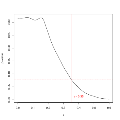
Figure 2: Left panel: Fitted dose response curves for male (linear model) and female (Emax model) patients from the IBS case study. Right panel: $p$-values of the test (4.8) for different values of the threshold $\varepsilon_{\infty}$ in the hypothesis (4.6).

The plateau of the curve is a consequence of the special construction of the test. If $\varepsilon_{\infty}\leq d_{\infty}=0.1784$, the constrained estimators in (3.14) coincide with the unconstrained estimators and consequently the bootstrap data is generated with the same parameters for each of these different values of $\varepsilon_{\infty}$.

In comparison, using the test of Gsteiger et al., (2011) discussed in Section 5, the maximum (minimum) of the upper (lower) confidence band is given by $0.282$ ($-0.450$) and $0.227$ $(-0.390)$ for $\alpha=0.05$ and $\alpha=0.1$ respectively. Thus, the null hypothesis cannot be rejected at either of these two significance levels as the bands are not completely contained in the rectangle $\mathcal{X}\times[-\varepsilon_{\infty},\varepsilon_{\infty}]$. Therefore, similarity of the curves at a significance level of $\alpha=0.1$ can only be claimed if $\varepsilon_{\infty}$ is larger than $0.390$. This illustrates again that the test proposed in Gsteiger et al., (2011) is conservative.
It might be also of interest to compare both curves with respect to the squared $L^{2}-$distance (2.4), which is given by $d_{2}(\hat{\beta}_{1},\hat{\beta}_{2})=0.0126$ for the IBS data. The $0.05$ and $0.1$ quantile of the bootstrap distribution are given by $q_{0.05,2}=0.0108$ and $q_{0.1,2}=0.0169$, respectively, for a choice of $\varepsilon_{2}=0.05$. Thus, we can reject the null hypothesis (3.1) at significance level $\alpha=0.1$ but not at $\alpha=0.05$. In this case the $p$-value is given by $0.059$. Finally, we illustrate the application of the asymptotic test (3.12). The variance estimator defined in (3.10) is given by $\hat{\sigma}_{d_{2}}^{2}=0.0010$ and for $\varepsilon_{2}=0.05$ we obtain the critical values $-0.0022$ ($\alpha=0.05$) and $0.0093$ ($\alpha=0.1$) for the test (3.12). Therefore the null hypothesis cannot be rejected at either of these two significance levels and the corresponding $p$-value is given by $0.1193$. These findings coincide with the results of the simulation study, which shows that the bootstrap test (3.17) is more accurate.

Acknowledgements This work has been supported in part by the Collaborative Research Center ”Statistical modeling of nonlinear dynamic processes” (SFB 823, Project C1) of the German Research Foundation (DFG). Kathrin Möllenhoff’s research has received funding from the European Union Seventh Framework Programme [FP7 2007–2013] under grant agreement no 602552 (IDEAL - Integrated Design and Analysis of small population group trials). The authors would like to thank Martina Stein, who typed parts of this manuscript with considerable technical expertise. We are very grateful to two referees, the associate editor and the editor for their constructive comments, which led to substantial improvement of an earlier version of this manuscript.

7 Appendix: Technical details

The theoretical results of this paper are proved under the following assumptions.

Assumption 7.1.

The errors $\eta_{\ell,i,j}$ are independent, have finite variance $\sigma_{\ell}^{2}$ and expectation zero.

Assumption 7.2.

The covariate region $\mathcal{X}\subset\mathbb{R}^{d}$ is compact and the number and location of dose levels $k_{\ell}$ does not depend on $n_{\ell},\ \ell=1,2$.

Assumption 7.3.

All estimators of the parameters $\beta_{1},\beta_{2}$ are computed over compact sets $B_{1}\subset\mathbb{R}^{p_{1}}$ and $B_{2}\subset\mathbb{R}^{p_{2}}$.

Assumption 7.4.

The regression functions $m_{1}$ and $m_{2}$ are twice continuously differentiable with respect to the parameters for all $b_{1},b_{2}$ in neighbourhoods of the true parameters $\beta_{1},\beta_{2}$ and all $x\in\mathcal{X}$. The functions $(x,b_{\ell})\mapsto m_{\ell}(x,b_{\ell})$ and their first two derivatives are continuous on $\mathcal{X}\times B_{\ell}$.

Assumption 7.5.

Defining $\psi_{a,\ell}^{(n)}(b):=\sum_{i=1}^{k_{\ell}}\frac{n_{\ell,i}}{n_{\ell}}(m_{\ell}(x_{\ell,i},a)-m_{\ell}(x_{\ell,i},b))^{2},$ we assume that for any $u>0$ there exists a constant $v_{u,\ell}>0$ such that

$$\liminf_{n_{1},n_{2}\to\infty}\inf_{a\in B_{\ell}}\inf_{|b-a|\geq u}\psi_{a,\ell}^{(n)}(b)\geq v_{u,\ell}\qquad\ell=1,2.$$

In particular, under Assumptions 7.1 - 7.5 the least squares estimator can be linearized. To be precise, consider arbitrary sequences $(\beta_{\ell,n})_{n\in\mathbb{N}}$ and $(\sigma_{\ell,n})_{n\in\mathbb{N}}$ in $B_{\ell}$ and $\mathbb{R}^{+}$ such that $\beta_{\ell,n}\to\beta_{\ell}$ and $\sigma_{\ell,n}\to\sigma_{\ell}>0$ as $n_{1},n_{2}\to\infty$ ($\ell=1,2$) and denote by $Y_{\ell,i,j}^{(n)}$ data of the form given in (2.1) with $\beta_{\ell}$ replaced by $\beta_{\ell,n}$ and $\eta_{\ell,i,j}$ independent and identically distributed (for each fixed $n$) with mean $0$ and finite variances $\sigma_{\ell,n}^{2}$. Then the least squares estimators $\hat{\beta}_{\ell}^{(n)}$ computed from $Y_{\ell,i,j}^{(n)}$ satisfy

$$\sqrt{n_{\ell}}\ (\hat{\beta}_{\ell}^{(n)}-\beta_{\ell,n})=\frac{1}{\sqrt{n_{\ell}}}\sum^{k_{\ell}}_{i=1}\sum^{n_{\ell,i}}_{j=1}\phi_{\ell,i,j}+o_{\mathbb{P}}(1),\qquad\ell=1,2,$$ (7.1)

where the functions $\phi_{\ell,i,j}^{(n)}$ are given by

$$\phi_{\ell,i,j}=\tfrac{\eta_{\ell,i,j}}{\sigma^{2}_{\ell,n}}\Sigma^{-1}_{\ell,n}\tfrac{\partial}{\partial b_{l}}m_{\ell}(x_{\ell,i},b_{\ell})\big{|}_{b_{l}=\beta_{\ell,n}},\qquad\ell=1,2,$$ (7.2)

and $\Sigma_{\ell,n}$ takes the form

$$\Sigma_{\ell,n}={1\over\sigma_{\ell,n}^{2}}\sum_{i=1}^{k_{\ell}}\zeta_{\ell,i}\tfrac{\partial}{\partial b_{l}}m_{\ell}(x_{\ell,i},b_{\ell})\big{|}_{b_{l}=\beta_{\ell,n}}\big{(}\tfrac{\partial}{\partial b_{l}}m_{\ell}(x_{\ell,i},b_{\ell})\big{|}_{b_{l}=\beta_{\ell,n}}\big{)}^{T}~{},~{}~{}\ell=1,2.$$ (7.3)

Proof of Theorem 3.1:

Let $\ell_{\infty}(\mathcal{X})$ denote the space of all bounded real valued functions of the form $g:\mathcal{X}\to\mathbb{R}$. The mapping $\Phi:\mathbb{R}^{p_{1}+p_{2}}\rightarrow\ell_{\infty}(\mathcal{X})$ defined by

$$(\theta_{1},\theta_{2})\mapsto\Phi(\theta_{1},\theta_{2}):\left\{\begin{array}[]{l}\mathcal{X}\mapsto\mathbb{R}\\ x\mapsto\big{(}\tfrac{\partial}{\partial b_{1}}m_{1}(x,b_{1})\big{|}_{b_{1}=\beta_{1}}\big{)}^{T}\theta_{1}-\big{(}\tfrac{\partial}{\partial b_{2}}m_{2}(x,b_{2})\big{|}_{b_{2}=\beta_{2}}\big{)}^{T}\theta_{2}\end{array}\right.$$ (7.4)

is continuous due to Assumptions 7.2-7.4, where we use the Euclidean and the supremum norm on $\mathbb{R}^{p_{1}+p_{2}}$ and $\ell_{\infty}(\mathcal{X})$, respectively. Consequently, the continuous mapping theorem [see Van der Vaart, (1998)] and (3.7) yield that the process

$$\{\sqrt{n}G_{n}(x)\}_{x\in\mathcal{X}}~{}:=\big{\{}\sqrt{n}\big{(}(\tfrac{\partial}{\partial b_{1}}m_{1}(x,b_{1})\big{|}_{b_{1}=\beta_{1}})^{T}(\hat{\beta_{1}}-\beta_{1})-(\tfrac{\partial}{\partial b_{2}}m_{2}(x,b_{2})\big{|}_{b_{2}=\beta_{2}})^{T}(\hat{\beta_{2}}-\beta_{2})\big{)}\big{\}}_{x\in\mathcal{X}}$$

converges weakly to a centered Gaussian process $\{G(x)\}_{x\in\mathcal{X}}$ in $\ell_{\infty}(\mathcal{X})$, which is defined by

$$G(x)=\big{(}\tfrac{\partial}{\partial b_{1}}m_{1}(x,b_{1})\big{|}_{b_{1}=\beta_{1}}\big{)}^{T}\sqrt{\lambda}\Sigma_{1}^{-1/2}Z_{1}-\big{(}\tfrac{\partial}{\partial b_{2}}m_{2}(x,b_{2})\big{|}_{b_{2}=\beta_{2}}\big{)}^{T}\sqrt{\tfrac{\lambda}{\lambda-1}}\Sigma_{2}^{-1/2}Z_{2},$$ (7.5)

where $Z_{1}$ and $Z_{2}$ are independent $p_{1}$- and $p_{2}$-dimensional standard normal distributed random variables, respectively, i.e. $Z_{\ell}\sim{\cal N}(0,I_{p_{\ell}})$, $\ell=1,2$. A straightforward calculation shows that the covariance kernel of the process $\{G(x)\}_{x\in\mathcal{X}}$ is given by (3.11). Now a Taylor expansion gives

$$p_{n}(x):=\big{(}m_{1}(x,\hat{\beta}_{1})-m_{1}(x,\beta_{1})\big{)}-\big{(}m_{2}(x,\hat{\beta}_{2})-m_{2}(x,\beta_{2})\big{)}=G_{n}(x)+o_{\mathbb{P}}\Big{(}\sqrt{\frac{1}{n}}\Big{)},$$ (7.6)

uniformly with respect to $x\in\mathcal{X}$, and it therefore follows that

$$\{\sqrt{n}p_{n}(x)\}_{x\in\mathcal{X}}\stackrel{{\scriptstyle\mathcal{D}}}{{\longrightarrow}}\left\{G(x)\right\}_{x\in\mathcal{X}}.$$ (7.7)

Recalling the definition of $\Delta(x,\beta_{1},\beta_{2})$ in (2.5), observing the representation

$$\sqrt{n}(\hat{d}_{2}-d_{2}) = \sqrt{n}\Big{(}\int_{\mathcal{X}}\Delta^{2}(x,\hat{\beta}_{1},\hat{\beta}_{2})dx-\int_{\mathcal{X}}\Delta^{2}(x,\beta_{1},\beta_{2})dx\Big{)}$$

$$= \int_{\mathcal{X}}\sqrt{n}p_{n}^{2}(x)dx+2\sqrt{n}\int_{\mathcal{X}}\Delta(x,\beta_{1},\beta_{2})p_{n}(x)dx,$$

and from the continuous mapping theorem we obtain $\sqrt{n}(\hat{d}_{2}-d_{2})\stackrel{{\scriptstyle\mathcal{D}}}{{\rightarrow}}2\int_{\mathcal{X}}\Delta(x,\beta_{1},\beta_{2})G(x)dx$, where $G$ denotes the Gaussian process defined in (7.5). Now it is easy to see that the distribution on the right-hand side is a centered normal distribution with variance $\sigma^{2}_{d_{2}}$ defined in (3.10). This completes the proof of Theorem 3.1. $\Box$

Proof of Theorem 3.4:

Proof of (1). First we will determine the asymptotic distribution of the bootstrap estimators $\hat{\beta}^{*}_{1}$ and $\hat{\beta}^{*}_{2}$. Then we use similar arguments as given in the proof of Theorem 3.1 to derive the asymptotic distribution of the statistic $\hat{d}_{2}^{*}$ (appropriately standardized). Finally, in a third step, we establish the statement $\eqref{level}$.
Recall the definition of the estimators in (3.14) and note that it follows from Assumptions 7.1-7.5 that $d_{2}\geq\varepsilon_{2}$ under the null hypothesis . We distinguish two cases. If $d_{2}>\varepsilon_{2}$, consistency of $\hat{\beta}_{\ell}$ implies that $\hat{d}_{2}>\varepsilon_{2}$ with probability tending to one, and thus $\hat{\hat{\beta_{\ell}}}=\hat{\beta}_{\ell}$ with probability tending to one. Next consider the case $d_{2}=\varepsilon_{2}$. Let $M:=\{(b_{1},b_{2})\in B_{1}\times B_{2}:d_{2}(b_{1},b_{2})=\varepsilon_{2}\}$ and note that $(\beta_{1},\beta_{2})\in M$. Define

$$\psi_{\ell}^{(n)}(b) := \sum_{i=1}^{k_{\ell}}\frac{n_{\ell,i}}{n_{\ell}}(m_{\ell}(x_{\ell,i},\beta_{\ell})-m_{\ell}(x_{\ell,i},b))^{2}~{},~{}\hat{\gamma}_{\ell}:=\frac{1}{n_{\ell}}\sum_{i=1}^{k_{\ell}}\sum_{j=1}^{n_{\ell,i}}(\eta_{\ell,i,j})^{2}$$

$$\hat{\psi}_{\ell}(b) := \frac{1}{n_{\ell}}\sum_{i=1}^{k_{\ell}}\sum_{j=1}^{n_{\ell,i}}(m_{\ell}(x_{\ell,i},\beta_{\ell})+\eta_{\ell,i,j}-m_{\ell}(x_{\ell,i},b))^{2}.$$

By definition (see (3.14) and (3.15)), we have $(\tilde{\beta}_{1},\tilde{\beta}_{2})=\arg\min_{(b_{1},b_{2})\in M}\sum_{\ell=1}^{2}\hat{\psi}_{\ell}(b_{\ell}).$ Moreover,

$$\arg\min_{(b_{1},b_{2})\in M}\sum_{\ell=1}^{2}\hat{\psi}_{\ell}(b_{\ell})=\arg\min_{(b_{1},b_{2})\in M}\sum_{\ell=1}^{2}(\hat{\psi}_{\ell}(b_{\ell})-\hat{\gamma}_{\ell}),$$

and

$$\hat{\psi}_{\ell}(b_{\ell})-\hat{\gamma}_{\ell}=\psi_{\ell}^{(n)}(b)+2\sum_{i=1}^{k_{\ell}}(m_{\ell}(x_{\ell,i},\beta_{\ell})-m_{\ell}(x_{\ell,i},b))\frac{1}{n_{\ell}}\sum_{j=1}^{n_{\ell,i}}\eta_{\ell,i,j}.$$

Observing that the terms $|m_{\ell}(x_{\ell,i},\beta_{\ell})-m_{\ell}(x_{\ell,i},b)|$ are uniformly bounded (with respect to $b\in B_{\ell}$ and $x_{\ell,i}\in{\cal X}$) it follows that

$$R_{n}:=\sum_{\ell=1}^{2}\sup_{b\in B_{\ell}}\Big{|}2\sum_{i=1}^{k_{\ell}}(m_{\ell}(x_{\ell,i},\beta_{\ell})-m_{\ell}(x_{\ell,i},b))\frac{1}{n_{\ell}}\sum_{j=1}^{n_{1,\ell}}\eta_{\ell,i,j}\Big{|}=o_{\mathbb{P}}(1)$$

since $\max_{i=1,...,k_{1}}|\frac{1}{n_{\ell}}\sum_{j=1}^{n_{\ell,i}}\eta_{\ell,i,j}|=o_{\mathbb{P}}(1)$. By similar arguments as given after (7.15), we obtain $|\tilde{\beta}_{\ell}-\beta_{\ell}|=o_{\mathbb{P}}(1)$, $\ell=1,2$ (recall that $(\beta_{1},\beta_{2})\in M$). Since for $\ell=1,2$ we have $|\hat{\hat{\beta_{\ell}}}-\beta_{\ell}|\leq|\hat{\beta}_{\ell}-\beta_{\ell}|+|\tilde{\beta}_{\ell}-\beta_{\ell}|$ and it follows from consistency of $\hat{\beta}_{\ell}$ that

$${\hat{\hat{\beta}}_{\ell}}\stackrel{{\scriptstyle\mathbb{P}}}{{\longrightarrow}}\beta_{\ell}\quad\ell=1,2,\quad\mbox{whenever}\quad d_{2}\geq\varepsilon_{2}.$$ (7.8)

For $\ell=1,2$ let ${\cal Y}_{\ell}=\sigma(Y_{\ell,i,j}|i=1,\ldots,k_{\ell},j=1,\ldots,n_{\ell,i})$ denote the $\sigma$-field generated by the random variables $\{Y_{\ell,i,j}|i=1,\ldots,k_{\ell},j=1,\ldots,n_{\ell,i}\}$ and ${\cal Y}:=\sigma({\cal Y}_{1},{\cal Y}_{2})$ (note that we do not display the dependence of these quantities on the sample size). Given (7.8) and the consistency of $\hat{\sigma}_{\ell}$, the discussion after Assumption 7.5 yields

$$\sqrt{n_{\ell}}(\hat{\beta}_{\ell}^{*}-\hat{\hat{\beta}}_{\ell})=\sum_{i=1}^{k_{\ell}}\frac{1}{\hat{\sigma}_{\ell}}\hat{\hat{\Sigma}}^{-1}_{\ell}\tfrac{\partial}{\partial\beta_{\ell}}m_{\ell}(x_{\ell,i,},\beta_{\ell})\big{|}_{\beta_{\ell}=\hat{\hat{\beta}}_{\ell}}\frac{1}{\sqrt{n_{\ell}}}\sum_{j=1}^{n_{\ell,i}}\tfrac{\eta^{*}_{\ell,i,j}}{\hat{\sigma}_{\ell}}~{}+~{}o_{\mathbb{P}}(1)~{},~{}~{}\ell=1,2.$$

where the $p_{1}\times p_{1}$ and $p_{2}\times p_{2}$ dimensional matrices $\hat{\hat{\Sigma}}^{-1}_{1}$ and $\hat{\hat{\Sigma}}^{-1}_{2}$ are defined by

$$\hat{\hat{\Sigma}}_{\ell}=\frac{1}{\hat{\sigma}^{2}_{\ell}}\sum^{k_{\ell}}_{i=1}\zeta_{\ell,i}\big{(}\tfrac{\partial}{\partial\beta_{\ell}}m_{\ell}(x_{\ell,i,},\beta_{\ell})\big{|}_{\beta_{\ell}=\hat{\hat{\beta}}_{\ell}}\big{)}\big{(}\tfrac{\partial}{\partial\beta_{\ell}}m_{\ell}(x_{\ell,i,},\beta_{\ell})\big{|}_{\beta_{\ell}=\hat{\hat{\beta}}_{\ell}}\big{)}^{T}.$$

Since by construction the $\frac{\eta^{*}_{\ell,i,j}}{\hat{\sigma}_{\ell}}$ are i.i.d. with unit variance and independent of ${\cal Y}$, the classical central limit theorem implies that, conditionally on ${\cal Y}$ in probability

$$\sqrt{n_{\ell}}\cdot\Sigma_{\ell}^{\frac{1}{2}}(\hat{\beta}^{*}_{\ell}-\hat{\hat{\beta_{\ell}}})\overset{D}{\longrightarrow}\mathcal{N}(0,I_{p_{\ell}})~{},\qquad\ell=1,2,$$ (7.9)

where the matrix $\Sigma_{\ell}$ is defined in (3.4). Observing the definition of the statistic

$$\hat{d}^{*}_{2}=d_{2}(\hat{\beta}_{1}^{*},\hat{\beta}_{2}^{*})=\int_{\mathcal{X}}(m_{1}(x,\hat{\beta}_{1}^{*})-m_{2}(x,\hat{\beta}^{*}_{2}))^{2}dx,$$

it now follows by the same arguments as given in the proof of Theorem 3.1 that

$$\frac{\sqrt{n}}{\sigma_{d_{2}}}(\hat{d}_{2}^{*}-\hat{\hat{d_{2}}})\stackrel{{\scriptstyle\mathcal{D}}}{{\rightarrow}}\mathcal{N}(0,1)$$ (7.10)

conditionally on ${\cal Y}$ in probability. Now recall that $\hat{q}_{\alpha,2}$ is the $\alpha$-quantile of the bootstrap statistic $\hat{d}^{*}_{2}$ conditionally on ${\cal Y}$ and note that, almost surely,

$$\alpha=\mathbb{P}(\hat{d}^{*}_{2}<\hat{q}_{\alpha,2}|~{}{\cal Y})=\mathbb{P}\Big{(}\frac{\sqrt{n}(\hat{d}^{*}_{2}-\hat{\hat{d}}_{2})}{\sigma_{d_{2}}}<\frac{\sqrt{n}(\hat{q}_{\alpha,2}-\hat{\hat{d}}_{2})}{\sigma_{d_{2}}}\Big{|}~{}{\cal Y}\Big{)}.$$ (7.11)

Letting $\hat{p}_{\alpha}:={\sqrt{n}(\hat{q}_{\alpha,2}-\hat{\hat{d}}_{2})}/{\sigma_{d_{2}}}$ it follows from $\eqref{bootstrapkonv}$, (7.11) and Lemma 21.2 in Van der Vaart, (1998) that

$$\hat{p}_{\alpha}\stackrel{{\scriptstyle\mathbb{P}}}{{\longrightarrow}}u_{\alpha},$$ (7.12)

where $u_{\alpha}$ denotes the $\alpha$-quantile of the standard normal distribution. This relation implies for any $\alpha<0.5$ that

$$\lim_{n\rightarrow\infty}\mathbb{P}(\hat{q}_{\alpha,2}-\hat{\hat{d}}_{2}>0\ )=\lim_{n\rightarrow\infty}\mathbb{P}\left(\hat{p}_{\alpha}>0\right)=0.$$ (7.13)

After these preparations we are able to prove the first part of Theorem 3.4, i.e. we show that the bootstrap test has asymptotic level $\alpha$ as specified in (3.17). It follows from (3.14) that in the case $\hat{d}_{2}=d_{2}(\hat{\beta}_{1},\hat{\beta}_{2})\geq\varepsilon_{2}$ the constrained estimators $\hat{\hat{\beta}}_{1}$ and $\hat{\hat{\beta}}_{2}$ coincide with the unconstrained OLS-estimators $\hat{\beta_{1}}$ and $\hat{\beta}_{2}$, respectively. This yields in particular $\hat{\hat{d}}_{2}=d_{2}(\hat{\hat{\beta}}_{1},\hat{\hat{\beta}}_{2})=\hat{d}_{2}$ whenever $\hat{d}_{2}\geq\varepsilon_{2}$.

If $d_{2}>\varepsilon_{2}$ we have

$$\mathbb{P}(\hat{d}_{2}<\hat{q}_{\alpha,2}) = \mathbb{P}(\hat{d}_{2}<\hat{q}_{\alpha,2},\ \hat{d}_{2}\geq\varepsilon_{2})+\mathbb{P}(\hat{d}_{2}<\hat{q}_{\alpha,2},\ \hat{d}_{2}<\varepsilon_{2})$$

$$\leq \mathbb{P}(\hat{d}_{2}<\hat{q}_{\alpha,2},\ \hat{\hat{d}}_{2}=\hat{d}_{2})+\mathbb{P}(\hat{d}_{2}<\varepsilon_{2})$$

$$\leq \mathbb{P}(\hat{\hat{d}}_{2}<\hat{q}_{\alpha,2})+\mathbb{P}\Big{(}\frac{\sqrt{n}(\hat{d}_{2}-d_{2})}{\sigma_{d_{2}}}<\frac{\sqrt{n}(\varepsilon_{2}-d_{2})}{\sigma_{d_{2}}}\Big{)}.$$

Observing that $\varepsilon_{2}-d_{2}<0$, it now follows from Theorem 3.1 that the second term is of order $o(1)$. On the other hand, we have from $\eqref{quantile3}$ that the first term is of the same order, which gives $\lim_{n_{1},n_{2}\rightarrow\infty}\mathbb{P}(\hat{d_{2}}<\hat{q}_{\alpha,2})=0$ and proves the first part of Theorem 3.4 in the case $d_{2}>\varepsilon_{2}$.

For a proof of the corresponding statement in the case ${d}_{2}=\varepsilon_{2}$ we note that it follows again from (7.13)

$$\mathbb{P}(\hat{d}_{2}<\hat{q}_{\alpha,2}) = \mathbb{P}(\hat{d}_{2}<\hat{q}_{\alpha,2},\ \hat{d}_{2}\geq\varepsilon_{2})+\mathbb{P}(\hat{d}_{2}<\hat{q}_{\alpha,2},\ \hat{d}_{2}<\varepsilon_{2})$$ (7.14)

$$= \mathbb{P}(\hat{d}_{2}<\hat{q}_{\alpha,2},\ \hat{\hat{d}}_{2}=\hat{d}_{2})+\mathbb{P}(\hat{d}_{2}<\hat{q}_{\alpha,2},\ \hat{\hat{d}}_{2}=\varepsilon_{2})-\mathbb{P}(\hat{d}_{2}<\hat{q}_{\alpha,2},\hat{d}_{2}=\varepsilon_{2})$$

$$= \mathbb{P}(\hat{d}_{2}<\hat{q}_{\alpha,2},\ \hat{\hat{d}}_{2}=\hat{d}_{2})+\mathbb{P}(\hat{d}_{2}<\hat{q}_{\alpha,2},\ \hat{\hat{d}}_{2}=\varepsilon_{2})+o(1)$$

$$= \mathbb{P}\Big{(}\frac{\sqrt{n}(\hat{d}_{2}-d_{2})}{\sigma_{d_{2}}}<\frac{\sqrt{n}(\hat{q}_{\alpha,2}-\hat{\hat{d}}_{2})}{\sigma_{d_{2}}},\hat{\hat{d}}_{2}=\varepsilon_{2}\Big{)}+o(1)$$

$$= \mathbb{P}\Big{(}\frac{\sqrt{n}(\hat{d}_{2}-d_{2})}{\sigma_{d_{2}}}<\frac{\sqrt{n}(\hat{q}_{\alpha,2}-\hat{\hat{d}}_{2})}{\sigma_{d_{2}}}\Big{)}$$

$$~{}~{}~{}~{}~{}-\mathbb{P}\big{(}\hat{d}_{2}-d_{2}<\hat{q}_{\alpha,2}-\hat{\hat{d}}_{2},\ \hat{\hat{d}}_{2}>\varepsilon_{2}\big{)}+o(1),$$

where the third equality is a consequence of the fact that $\sqrt{n}(\hat{d}_{2}-d_{2})$ is asymptotically normal distributed, which gives $\mathbb{P}(\hat{d}_{2}<\hat{q}_{\alpha,2},\hat{d}_{2}=\varepsilon_{2})\leq\mathbb{P}(\hat{d}_{2}=\varepsilon_{2})=o(1).$ If ${\hat{\hat{d}}}_{2}>\varepsilon_{2}$ it follows that $\hat{d}_{2}={\hat{\hat{d}}}_{2}>\varepsilon_{2}=d_{2}$ and consequently the second term in (7.14) can be bounded by (observing again (7.13)) $\mathbb{P}(\hat{d}_{2}-d_{2}<\hat{q}_{\alpha,2}-{\hat{\hat{d}}}_{2},\hat{d}_{2}>\varepsilon_{2})\leq\mathbb{P}(\hat{q}_{\alpha,2}-{\hat{\hat{d}}}_{2}>0)=o(1).$ Therefore we obtain from Theorem 3.1, $\eqref{quantile2}$ and (7.14) that $\lim_{n\rightarrow\infty}\mathbb{P}(\hat{d}_{2}<\hat{q}_{\alpha,2})=\Phi(u_{\alpha})=\alpha,$ which completes the proof of part (1) of Theorem 3.4.

Proof of (2). Finally, we consider the case $d_{2}<\varepsilon_{2}$ and show the consistency of the test (3.17). Theorem 3.1 implies that $\hat{d}_{2}{\stackrel{{\scriptstyle\mathbb{P}}}{{\longrightarrow}}}d_{2}$. Since $d_{2}<\varepsilon_{2}$, there exists a constant $\delta>0$ such that $\mathbb{P}(\hat{d}_{2}<\varepsilon_{2}-\delta)\to 1$. Hence the assertion will follow if we establish that $\mathbb{P}(\hat{q}_{\alpha,2}>\varepsilon_{2}-\delta)\to 1$. To show this, denote by $F_{b_{1},b_{2},s_{1},s_{2}}^{(n)}$ the conditional distribution function of $\hat{d}^{*}_{2}$ given ${\hat{\hat{\beta}}}_{\ell}=b_{\ell},\hat{\sigma}_{\ell}=s_{\ell}\ (\ell=1,2)$. Since $\mathbb{P}(\max_{\ell=1,2}|\hat{\sigma}_{\ell}-\sigma_{\ell}|\leq r)\to 1$ for any $r>0$, it suffices to establish that for some $r>0$

$$\sup\big{\{}F_{b_{1},b_{2},s_{1},s_{2}}^{(n)}(\varepsilon_{2}-\delta)\mid b_{\ell}\in B_{\ell},\ell=1,2;\max_{\ell=1,2}|s_{\ell}-\sigma_{\ell}|\leq r\big{\}}\to 0.$$

By uniform continuity of the map $(b_{1},b_{2})\mapsto d_{2}(b_{1},b_{2})$ it suffices to prove that for all $\eta>0$ and $\ell=1,2$

$$\sup\Big{\{}\mathbb{P}(|\hat{\beta}_{\ell}^{*}-b_{\ell}|\geq\eta\mid\hat{\hat{\beta}}_{k}=b_{k},\hat{\sigma}_{k}=s_{k},k=1,2)\Big{|}~{}{(b_{\ell},s_{\ell}):|s_{\ell}-\sigma_{\ell}|\leq r,b_{\ell}\in B_{\ell},\ell=1,2}\Big{\}}\to 0.$$

(7.15)

We will only prove the above statement for $\ell=1$ since the case $\ell=2$ follows by exactly the same arguments. For $i=1,...,k_{1},j=1,...,n_{1,i}$ let $e_{i,j}$ i.i.d. $\sim\mathcal{N}(0,1)$ and define

$$\psi_{a,1}^{(n)}(b) := \sum_{i=1}^{k_{1}}\frac{n_{1,i}}{n_{1}}(m_{1}(x_{1,i},a)-m_{1}(x_{1,i},b))^{2}~{},~{}\hat{\gamma}_{s}:=\frac{1}{n_{1}}\sum_{i=1}^{k_{1}}\sum_{j=1}^{n_{1,i}}(se_{i,j})^{2}$$

$$\hat{\psi}_{a,s}(b) := \frac{1}{n_{1}}\sum_{i=1}^{k_{1}}\sum_{j=1}^{n_{1,i}}(m_{1}(x_{1,i},a)+se_{i,j}-m_{1}(x_{1,i},b))^{2}.$$

By construction, the conditional distribution of $\hat{\beta}_{1}^{*}$ given $\hat{\hat{\beta}}_{1}=a,\hat{\sigma}_{1}=s$ is equal to the distribution of the random variable $\hat{b}_{a,s}:=\arg\min_{b\in B_{1}}\hat{\psi}_{a,s}(b)$. On the other hand, $\arg\min_{b\in B_{1}}\hat{\psi}_{a,s}(b)=\arg\min_{b\in B_{1}}(\hat{\psi}_{a,s}(b)-\hat{\gamma}_{s})$, and

$$\hat{\psi}_{a,s}(b)-\hat{\gamma}_{s}=\psi_{a,1}^{(n)}(b)+2s\sum_{i=1}^{k_{1}}(m_{1}(x_{1,i},a)-m_{1}(x_{1,i},b))\frac{1}{n_{1}}\sum_{j=1}^{n_{1,i}}e_{i,j}.$$

Observing that the terms $|m_{1}(x_{1,i},a)-m_{1}(x_{1,i},b)|$ are uniformly bounded (with respect to $a,b\in B_{1}$ and $x_{1,i}\in{\cal X}$) it follows that

$$R_{n}:=\sup_{|s-\sigma_{1}|\leq r}\sup_{a,b\in B_{1}}\Big{|}2s\sum_{i=1}^{k_{1}}(m_{1}(x_{1,i},a)-m_{1}(x_{1,i},b))\frac{1}{n_{1}}\sum_{j=1}^{n_{1,i}}e_{i,j}\Big{|}=o_{\mathbb{P}}(1)$$

since $\max_{i=1,...,k_{1}}|\frac{1}{n_{1}}\sum_{j=1}^{n_{1,i}}e_{i,j}|=o_{\mathbb{P}}(1)$. Now we obtain from Assumption 7.5 that, for sufficiently large $n$,

$$\sup_{(a,s):|s-\sigma_{1}|\leq r}\mathbb{P}(|\hat{\beta}_{1}^{*}-a|\geq\eta|\hat{\hat{\beta}}_{1}=a,\hat{\sigma}_{1}=s)\leq\sup_{(a,s):|s-\sigma_{1}|\leq r}\mathbb{P}(|\hat{b}_{a,s}-a|\geq\eta) \leq \mathbb{P}(R_{n}\geq v_{\eta}/4)=o(1).$$

Thus (7.15) follows, which completes the proof of Theorem 3.4. $\Box$

Proof of Theorem 4.1:

Recall the definition of the estimator $\hat{d}_{\infty}$ in (4.1) and define the random variables

$$D_{n} = \sqrt{n}\ (\hat{d}_{\infty}-d_{\infty})=\sqrt{n}\ \big{(}\max_{x\in\mathcal{X}}|m_{1}(x,\hat{\beta}_{1})-m_{2}(x,\hat{\beta}_{2})|-d_{\infty}\big{)},$$ (7.16)

$$Z_{n} = \sqrt{n}\ \big{(}\max_{x\in\mathcal{E}}|m_{1}(x,\hat{\beta}_{1})-m_{2}(x,\hat{\beta}_{2})|-d_{\infty}\big{)}.$$ (7.17)

We will use similar arguments as given in Raghavachari, (1973) and show that

$$R_{n}=D_{n}-Z_{n}=o_{\mathbb{P}}(1),$$ (7.18)

$$Z_{n}\stackrel{{\scriptstyle\cal D}}{{\longrightarrow}}\mathcal{Z},$$ (7.19)

which proves the assertion of Theorem 4.1. For a proof of (7.18) we recall the definition of the ”true” difference $\Delta(x,\beta_{1},\beta_{2})$ in (2.5) and the definition of the process $\{p_{n}(x)\}_{x\in\mathcal{X}}$ in (7.6). It follows from (7.7) and the continuous mapping theorem that

$$\lim_{n_{1},n_{2}\to\infty}\mathbb{P}\big{(}\max_{x\in\mathcal{X}}|p_{n}(x)|>a_{n}\big{)}=0$$ (7.20)

as $n_{1},n_{2}\to\infty,\ n/n_{1}\to\lambda\in(1,\infty)$, where $a_{n}={\log n}/{\sqrt{n}}$. By the representation $p_{n}(x)=G_{n}(x)+o_{\mathbb{P}}(n^{-1/2})$ uniformly in $x\in\mathcal{X}$ and the definition of $G_{n}$ in (7.6) we have for every $\eta>0$

$$\lim_{\delta\downarrow 0}\lim_{n_{1},n_{2}\to\infty}\mathbb{P}\Big{(}\sup_{\|x-y\|<\delta}\sqrt{n}|p_{n}(x)-p_{n}(y)|>\eta\Big{)}=0,$$ (7.21)

where $\|\cdot\|$ denotes a norm on $\mathcal{X}\subset\mathbb{R}^{d}$. In the following discussion define the sets

$$\mathcal{E}^{\mp}_{n}=\big{\{}x\in\mathcal{X}\mid|\mp d_{\infty}-\Delta(x,\beta_{1},\beta_{2})|\leq a_{n}\big{\}}$$ (7.22)

and $\mathcal{E}_{n}=\mathcal{E}^{+}_{n}\cup\mathcal{E}^{-}_{n}$, then it follows from the definition of $R_{n}$ and (7.20) that

$$0\leq R_{n} = \sqrt{n}\Big{(}\max_{x\in\mathcal{X}}|\Delta(x,\hat{\beta}_{1},\hat{\beta}_{2})|-\max_{x\in\mathcal{E}}|\Delta(x,\hat{\beta}_{1},\hat{\beta}_{2})|\Big{)}$$

$$= \sqrt{n}\Big{(}\max_{x\in\mathcal{E}_{n}}|\Delta(x,\hat{\beta}_{1},\hat{\beta}_{2})|-\max_{x\in\mathcal{E}}|\Delta(x,\hat{\beta}_{1},\hat{\beta}_{2})|\Big{)}+o_{\mathbb{P}}(1)$$

$$\leq \max(R^{-}_{n},R^{+}_{n})+o_{\mathbb{P}}(1),$$

where $R^{\mp}_{n}=\sqrt{n}\big{(}\max_{x\in\mathcal{E}^{\mp}_{n}}|\Delta(x,\hat{\beta}_{1},\hat{\beta}_{2})|-\max_{x\in\mathcal{E}^{\mp}}|\Delta(x,\hat{\beta}_{1},\hat{\beta}_{2})|\big{)}.$ We now prove the estimate $R^{\mp}_{n}=o_{\mathbb{P}}(1)$, which completes the proof of assertion (7.18). For this purpose we restrict ourselves to the random variable $R^{+}_{n}$ (the assertion for $R^{-}_{n}$ is obtained by similar arguments). Note that $\mathcal{E}^{+}\subset\mathcal{E}^{+}_{n}$ and therefore it follows that

$$0\leq R^{+}_{n} = \sqrt{n}\Big{(}\max_{x\in\mathcal{E}^{+}_{n}}\Delta(x,\hat{\beta}_{1},\hat{\beta}_{2})-\max_{x\in\mathcal{E}^{+}}\Delta(x,\hat{\beta}_{1},\hat{\beta}_{2})\Big{)}+o_{\mathbb{P}}(1)$$

$$\leq \max_{x\in\mathcal{E}^{+}_{n}}\sqrt{n}p_{n}(x)-\max_{x\in\mathcal{E}^{+}}\sqrt{n}p_{n}(x)+\sqrt{n}\Big{\{}\max_{x\in\mathcal{E}^{+}_{n}}\Delta(x,\beta_{1},\beta_{2})-d_{\infty}\Big{\}}+o_{\mathbb{P}}(1)$$

$$= \max_{x\in\mathcal{E}^{+}_{n}}\sqrt{n}p_{n}(x)-\max_{x\in\mathcal{E}^{+}}\sqrt{n}p_{n}(x)+o_{\mathbb{P}}(1).$$

Now define for $\gamma>0$ the set $\mathcal{E}^{+}(\gamma)=\{x\in\mathcal{X}\mid\exists\ y\in\mathcal{E}^{+}\quad\mbox{with}\quad\|x-y\|<\gamma\}$ and the constant $\delta_{n}=2\inf\{\gamma>0\mid\mathcal{E}^{+}_{n}\subset\mathcal{E}^{+}(\gamma)\}$. Obviously $\mathcal{E}^{+}_{n}\subset\mathcal{E}^{+}(\delta_{n})$ and the sequence $(\delta_{n})_{n\in\mathbb{N}}$ is decreasing, such that $\delta:=\lim_{n\to\infty}\delta_{n}$ exists. By the definition of $\delta_{n}$ we have $\mathcal{E}^{+}_{n}\not\subset\mathcal{E}^{+}({\delta_{n}/4})$. Consequently, there exist $x_{n}\in\mathcal{E}^{+}_{n}\subset\mathcal{X}$ such that $\|x_{n}-y\|\geq{\delta_{n}/4}$ for all $y\in\mathcal{E}^{+}$ and all $n\in\mathbb{N}$. The sequence $(x_{n})_{n\in\mathbb{N}}$ contains a convergent subsequence (because $\mathcal{X}$ is compact), say $(x_{n_{k}})_{k\in\mathbb{N}}$ which satisfies $\lim_{k\to\infty}x_{n_{k}}=x\in\mathcal{X},$ $d_{\infty}=\lim_{k\to\infty}\Delta(x_{n_{k}},\beta_{1},\beta_{2})=\Delta(x,\beta_{1},\beta_{2}).$ Consequently, $x\in\mathcal{E}^{+}$, but by construction $\|x_{n_{k}}-x\|\geq{\delta_{n}/4}$ for all $k\in\mathbb{N}$, which is only possible if $\delta=\lim_{n\to\infty}\delta_{n}=0$.

Now it follows from inequality (7) for the sequence $(\delta_{n})_{n\in\mathbb{N}}$

$$o_{\mathbb{P}}(1)\leq R^{+}_{n} \leq \max_{x\in\mathcal{E}^{+}(\delta_{n})}\sqrt{n}p_{n}(x)-\max_{x\in\mathcal{E}^{+}}\sqrt{n}p_{n}(x)+o_{\mathbb{P}}(1)$$

$$\leq \max_{\|y-x\|\leq\delta_{n}}\sqrt{n}|p_{n}(x)-p_{n}(y)|+o_{\mathbb{P}}(1)=o_{\mathbb{P}}(1),$$

where the last estimate is a consequence of (7.21). A similar statement for $R^{-}_{n}$ completes the proof of (7.18).

For a proof of the second assertion (7.19) we define the random variable

$$\tilde{Z}_{n}=\max\big{\{}\max_{x\in\mathcal{E}^{+}}\sqrt{n}p_{n}(x);\ \max_{x\in\mathcal{E}^{-}}(-\sqrt{n}p_{n}(x))\big{\}},$$

then it follows from (7.7) and the continuous mapping theorem that $\tilde{Z}_{n}\stackrel{{\scriptstyle\mathcal{D}}}{{\longrightarrow}}\mathcal{Z}$, where the random variable $\mathcal{Z}$ is defined in (4.4). Observing the uniform convergence in (7.20) we have as $n_{1},n_{2}\to\infty$

$$\mathbb{P}(Z_{n}\leq t) = \mathbb{P}\big{(}Z_{n}\leq t,\ \max_{x\in\mathcal{X}}|p_{n}(x)|<\tfrac{d_{\infty}}{2}\big{)}+o(1)=\mathbb{P}\big{(}{\tilde{Z}_{n}\leq t},\ \max_{x\in\mathcal{X}}|p_{n}(x)|<\tfrac{d_{\infty}}{2}\big{)}+o(1)$$

$$= \mathbb{P}(\tilde{Z}_{n}\leq t)+o(1)=\mathbb{P}(\mathcal{Z}\leq t)+o(1).$$

This proves the remaining statement and completes the proof of Theorem 4.1. $\Box$

Proof of Theorem 4.2:

We begin by noting that the statement (4.11) follows by exactly the same arguments as given in the proof of (3.19) in Theorem 3.4 once we note that the mapping $(b_{1},b_{2})\mapsto d_{\infty}(b_{1},b_{2})$ is uniformly continuous. The details are omitted for the sake of brevity.
Throughout the remaining proof, let $\hat{\hat{\beta_{1}}}$ and $\hat{\hat{\beta_{2}}}$ denote the estimators defined by

$${\hat{\hat{\beta}}_{\ell}}=\left\{\begin{array}[]{ccc}\hat{\beta}_{\ell}&\mbox{if}&\hat{d}_{\infty}\geq\varepsilon_{\infty}\\ \tilde{\beta}_{\ell}&\mbox{if}&\hat{d}_{\infty}<\varepsilon_{\infty}\end{array}\right.\quad\ell=1,2,$$

where $\tilde{\beta}_{1},\tilde{\beta}_{2}$ denote the OLS-estimators of the parameters $\beta_{1},\beta_{2}$ under the constraint $d_{\infty}(\beta_{1},\beta_{2})=\varepsilon_{\infty}$ and define

$$p_{n}^{*}(x) := \big{(}m_{1}(x,\hat{\beta}^{*}_{1})-m_{1}(x,\hat{\hat{\beta}}_{1})\big{)}-\big{(}m_{2}(x,\hat{\beta}^{*}_{2})-m_{2}(x,\hat{\hat{\beta}}_{2})\big{)},$$

$$G_{n}^{*}(x) = (\tfrac{\partial}{\partial b_{1}}m_{1}(x,b_{1})\big{|}_{b_{1}=\hat{\hat{\beta}}_{1}})^{T}(\hat{\beta}_{1}^{*}-\hat{\hat{\beta_{1}}})-(\tfrac{\partial}{\partial b_{2}}m_{2}(x,b_{2})\big{|}_{b_{2}=\hat{\hat{\beta}}_{2}})^{T}(\hat{\beta}^{*}_{2}-\hat{\hat{\beta}}_{2}).$$

Similarly to the proof of Theorem 3.1, it is possible to establish that

$${\hat{\hat{\beta}}_{\ell}} \stackrel{{\scriptstyle\mathbb{P}}}{{\longrightarrow}} \beta_{\ell}\quad\ell=1,2,\quad\mbox{whenever}\quad d_{\infty}\geq\varepsilon_{\infty},$$ (7.24)

$$\left\{\sqrt{n}p_{n}^{*}(x)\right\}_{x\in\mathcal{X}} \stackrel{{\scriptstyle\mathcal{D}}}{{\longrightarrow}} \left\{G(x)\right\}_{x\in\mathcal{X}}$$ (7.25)

$$p_{n}^{*}(x) = G_{n}^{*}(x)+o_{\mathbb{P}}(n^{-1/2})$$ (7.26)

uniformly with respect to $x\in\mathcal{X}$, where $\left\{G(x)\right\}_{x\in\mathcal{X}}$ denotes the Gaussian process defined in (7.5). Here, the weak convergence in (7.25) holds conditionally on ${\cal Y}$ in probability as well as unconditionally.

From now on assume that the null hypothesis $d_{\infty}\geq\varepsilon_{\infty}$ is satisfied, and define

$$\mathcal{F}_{n}^{\mp*} = \big{\{}x\in\mathcal{X}\mid m_{1}(x,\hat{\beta}_{1}^{*})-m_{2}(x,\hat{\beta}_{2}^{*})=\mp\hat{d}_{\infty}^{*}\big{\}},$$

$$\mathcal{E}_{n}^{\mp} = \big{\{}x\in\mathcal{X}\mid m_{1}(x,\hat{\hat{\beta}}_{1})-m_{2}(x,\hat{\hat{\beta}}_{2})=\mp\hat{\hat{d}}_{\infty}\big{\}},$$

where

$$\hat{d}_{\infty}^{*} = \sup_{x\in{\cal X}}|m_{1}(x,\hat{\beta}_{1}^{*})-m_{2}(x,\hat{\beta}_{2}^{*})|~{},~{}~{}\hat{\hat{d}}_{\infty}=\sup_{x\in{\cal X}}|m_{1}(x,\hat{\hat{\beta}}_{1})-m_{2}(x,\hat{\hat{\beta}}_{2})|~{}.$$

From (7.24) and the continuous mapping theorem we obtain the existence of a sequence $(\gamma_{n})_{\in\mathbb{N}}$ such that $\gamma_{n}\to 0$ and

$$\sup_{x\in\mathcal{X}}|\Delta(x,\hat{\hat{\beta}}_{1},\hat{\hat{\beta}}_{2})-\Delta(x,\beta_{1},\beta_{2})|=o_{\mathbb{P}}(\gamma_{n}),\ \sup_{x\in\mathcal{X}}|\Delta(x,\hat{\beta}^{*}_{1},\hat{\beta}^{*}_{2})-\Delta(x,\hat{\hat{\beta}}_{1},\hat{\hat{\beta}}_{2})|=o_{\mathbb{P}}(a_{n}),\quad$$ (7.27)

where $a_{n}=\log n/\sqrt{n}$ and the second statement follows from (7.25). Moreover, from the representation (7.25) we have for every $\eta>0$

$$\lim_{\delta\downarrow 0}\limsup_{n_{1},n_{2}\to\infty}\mathbb{P}\Big{(}\sqrt{n}\sup_{\|x-y\|<\delta}|p^{*}_{n}(x)-p^{*}_{n}(y)|>\eta\Big{)}=0.$$ (7.28)

Now define $b_{n}=\max\{\gamma_{n},a_{n}\}$ and consider the sets

$$\mathcal{F}_{n}^{\pm}=\{x\in{\cal X}~{}|~{}|\pm d_{\infty}-\Delta(x,\beta_{1},\beta_{2})|\leq b_{n}\}$$

and $\mathcal{F}_{n}=\mathcal{F}_{n}^{+}\cup\mathcal{F}_{n}^{-}$. Additionally, define the set

$$\mathcal{E}^{\pm}(\gamma)=\{x\in\mathcal{X}\mid\exists\ y\in\mathcal{E}^{\pm}\quad\mbox{with}\quad\|x-y\|<\gamma\}$$

for $\gamma>0$. At the end of the proof we shall show that there exists a sequence $\delta_{n}\to 0$ such that

$$\mathbb{P}\big{(}\mathcal{E}^{\pm}_{n}\cup\mathcal{F}^{\pm*}_{n}\subseteq\mathcal{F}_{n}^{\pm}\subseteq\mathcal{E}^{\pm}(\delta_{n})\big{)}\to 1.$$ (7.29)

In the special case $\#\mathcal{E}=1$ with $\mathcal{E}=\{x_{0}\}$ for some $x_{0}\in\mathcal{X}$ we shall prove that additionally

$$\sqrt{n}(\hat{d}_{\infty}^{*}-\hat{\hat{d}}_{\infty})\stackrel{{\scriptstyle\mathcal{D}}}{{\rightarrow}}G(x_{0})\quad\mbox{conditionally on ${\cal Y}$ in probability}.$$ (7.30)

Given (7.29) and (7.30) we prove (4.9) and (4.10). For a proof of (4.9) note that $\hat{q}_{\alpha,\infty}$ is the $\alpha$-quantile of the bootstrap test statistics $\hat{d}_{\infty}^{*}$ conditionally on ${\cal Y}$. Thus the $\alpha$-quantile of the distribution of $\sqrt{n}(\hat{d}_{\infty}^{*}-\hat{\hat{d}}_{\infty})$ conditionally on ${\cal Y}$ is of the form $\hat{p}_{\alpha,\infty}:=\sqrt{n}(\hat{q}_{\alpha,\infty}-\hat{\hat{d}}_{\infty})$ and, by (7.30), satisfies $\hat{p}_{\alpha,\infty}\stackrel{{\scriptstyle\mathbb{P}}}{{\longrightarrow}}z_{\alpha}$, where $z_{\alpha}$ denotes the $\alpha$-quantile of the distribution of $G(x_{0})$. With $\sigma^{2}_{d_{\infty}}:={\rm Var}(G(x_{0}))$, it now follows from Lemma 21.2 in Van der Vaart, (1998) ${\hat{p}_{\alpha}}/{\sigma_{d_{\infty}}}\stackrel{{\scriptstyle\mathbb{P}}}{{\longrightarrow}}u_{\alpha},$ where $u_{\alpha}$ denotes the $\alpha$-quantile of the standard normal distribution. This result is the analogue of (7.12) in the proof of Theorem 3.4, and (4.9) now follows by exactly the same arguments as given in the proof of (3.18) in Theorem 3.4.

Next, we derive a preliminary result that will be used to prove (4.10). Define for the sequence $\delta_{n}$ from (7.29)

$$\widetilde{\mathcal{Z}}^{*}_{n}:=\sqrt{n}\max\big{\{}\max_{x\in\mathcal{E}^{+}(\delta_{n})}p_{n}^{*}(x),\max_{x\in\mathcal{E}^{-}(\delta_{n})}(-p_{n}^{*}(x))\big{\}}.$$

From (7.29) we obtain

$$\hat{d}_{\infty}^{*}-\hat{\hat{d}}_{\infty} = \max_{x\in\mathcal{X}}|\Delta(x,\hat{\beta}_{1}^{*},\hat{\beta}_{2}^{*})|-\hat{\hat{d}}_{\infty}$$ (7.31)

$$= \max\{\max_{x\in\mathcal{E}^{+}(\delta_{n})}\Delta(x,\hat{\beta}_{1}^{*},\hat{\beta}_{2}^{*}),\max_{x\in\mathcal{E}^{-}(\delta_{n})}(-\Delta(x,\hat{\beta}_{1}^{*},\hat{\beta}_{2}^{*}))\}-\hat{\hat{d}}_{\infty}+o_{\mathbb{P}}(n^{-1/2}).\quad\quad\quad$$

Moreover,

$$\max_{x\in\mathcal{E}^{\pm}(\delta_{n})}(\pm\Delta(x,\hat{\beta}_{1}^{*},\hat{\beta}_{2}^{*})-\hat{\hat{d}}_{\infty})\leq\max_{x\in\mathcal{E}^{\pm}(\delta_{n})}(\pm\Delta(x,\hat{\beta}_{1}^{*},\hat{\beta}_{2}^{*})\mp\Delta(x,\hat{\hat{\beta}}_{1},\hat{\hat{\beta}}_{2}))$$

and thus

$$\sqrt{n}(\hat{d}_{\infty}^{*}-\hat{\hat{d}}_{\infty})\leq\widetilde{\mathcal{Z}}_{n}^{*}+o_{\mathbb{P}}(1).$$ (7.32)

Denoting by $\hat{p}_{\alpha,\infty}$ the $\alpha$-quantile of $\sqrt{n}(\hat{d}^{*}_{\infty}-\hat{\hat{d}}_{\infty})$ conditional on the data we have $\hat{q}_{\alpha,\infty}=\hat{\hat{d}}_{\infty}+n^{-1/2}\hat{p}_{\alpha,\infty}$.

Define $F_{n}^{*}$ as the distribution function of $\sqrt{n}(\hat{d}^{*}_{\infty}-\hat{\hat{d}}_{\infty})$ conditional on the data, $F_{n}$ as the distribution function of $\widetilde{\mathcal{Z}}_{n}^{*}$ conditional on the data and $F_{\mathcal{Z}}$ as the distribution function of $\mathcal{Z}$. By the definition of $\mathcal{Z}$ and the results in Tsirel’son, (1976) the function $F_{\mathcal{Z}}$ can have at most one jump, and this jump can only be located at its left support point. Since $F_{\mathcal{Z}}$ is continuous at $q_{\mathcal{Z},\alpha}$ and $q_{\mathcal{Z},\alpha}<0$ there exists $t_{0}<0$ such that $F_{\mathcal{Z}}(t_{0})<\alpha$ and $F_{\mathcal{Z}}$ is continuous on $[t_{0},\infty)$. Since $\widetilde{\mathcal{Z}}^{*}_{n}$ converges weakly to $\mathcal{Z}$ conditionally on the data in probability it follows that $\sup_{t\geq t_{0}}|F_{n}(t)-F_{\mathcal{Z}}(t)|=o_{\mathbb{P}}(1)$. From (7.32) we have $\mathbb{P}(F_{n}^{*}(t)\geq F_{n}(t-\varepsilon)~{}~{}\forall t)\to 1$ for any $\varepsilon>0$, and the uniform continuity of $F_{\mathcal{Z}}$ on $[t_{0},\infty)$ yields $\mathbb{P}(F_{n}^{*}(t)\geq F_{\mathcal{Z}}(t)-\varepsilon~{}~{}\forall t\geq t_{0})\to 1$ for any $\varepsilon>0$. Let $q_{\mathcal{Z},\alpha+\delta}$ denote the $\alpha+\delta$ quantile of $F_{\mathcal{Z}}$. For arbitrary $\delta>0$ it follows that $q_{\mathcal{Z},\alpha+\delta}>t_{0}$ and thus

$$o(1)=\mathbb{P}(F_{n}^{*}(q_{\mathcal{Z},\alpha+\delta})\geq F_{\mathcal{Z}}(q_{\mathcal{Z},\alpha+\delta})-\delta/3)=\mathbb{P}(F_{n}^{*}(q_{\mathcal{Z},\alpha+\delta})\geq\alpha+2\delta/3).$$

Thus, by definition of $\hat{p}_{\alpha,\infty}$, we have

$$\mathbb{P}(\hat{p}_{\alpha,\infty}>q_{\mathcal{Z},\alpha+\delta})=o(1)\quad\forall\delta>0.$$ (7.33)

Specifically, choosing $\delta>0$ with $q_{\mathcal{Z},\alpha+\delta}<0$ we obtain

$$\mathbb{P}(\hat{q}_{\alpha,\infty}>{\hat{\hat{d}}}_{\infty})=\mathbb{P}(\hat{p}_{\alpha,\infty}>0)=o(1).$$ (7.34)

Given (7.33) and (7.34) we are ready to prove (4.10). First consider the case ${d}_{\infty}=\varepsilon_{\infty}$ and note that it follows from (7.34) that

$$\mathbb{P}(\hat{d}_{\infty}<\hat{q}_{\alpha,\infty}) = \mathbb{P}(\hat{d}_{\infty}<\hat{q}_{\alpha,\infty},\ \hat{\hat{d}}_{\infty}=\varepsilon_{\infty})+\mathbb{P}(\hat{d}_{\infty}<\hat{q}_{\alpha,\infty},\hat{\hat{d}}_{\infty}>\varepsilon_{\infty})$$

$$= \mathbb{P}(\hat{d}_{\infty}<\hat{q}_{\alpha,\infty},\ \hat{\hat{d}}_{\infty}=\varepsilon_{\infty})+\mathbb{P}(\hat{\hat{d}}_{\infty}<\hat{q}_{\alpha,\infty},\hat{\hat{d}}_{\infty}>\varepsilon_{\infty})$$

$$= \mathbb{P}\Big{(}\sqrt{n}(\hat{d}_{\infty}-d_{\infty})<\sqrt{n}(\hat{q}_{\alpha,\infty}-\hat{\hat{d}}_{\infty}),\hat{\hat{d}}_{\infty}=\varepsilon_{\infty}\Big{)}+o(1)$$

$$\leq \mathbb{P}\Big{(}\sqrt{n}(\hat{d}_{\infty}-d_{\infty})<\sqrt{n}(\hat{q}_{\alpha,\infty}-\hat{\hat{d}}_{\infty})\Big{)}+o(1)$$

$$= \mathbb{P}\Big{(}\sqrt{n}(\hat{d}_{\infty}-d_{\infty})<\hat{p}_{\alpha,\infty}\Big{)}+o(1),$$

where the second equality follows since on the event $\hat{\hat{d}}_{\infty}>\varepsilon_{\infty}$ we have $\hat{\hat{d}}_{\infty}={\hat{d}}_{\infty}$ and the third equality follows from (7.34). From (7.33) we obtain for any $\delta>0$

$$\mathbb{P}\Big{(}\sqrt{n}(\hat{d}_{\infty}-d_{\infty})<\hat{p}_{\alpha,\infty}\Big{)}\leq\mathbb{P}\Big{(}\sqrt{n}(\hat{d}_{\infty}-d_{\infty})<q_{\mathcal{Z},\alpha+\delta}\Big{)}+o(1)\to\alpha+\delta$$

because the distribution of $\mathcal{Z}$ is continuous at $q_{\mathcal{Z},\alpha+\delta}$. Since $\delta>0$ was arbitrary (4.10) follows in the case ${d}_{\infty}=\varepsilon_{\infty}$.

Next consider the case ${d}_{\infty}>\varepsilon_{\infty}$. We have

$$\mathbb{P}(\hat{d}_{\infty}<\hat{q}_{\alpha,\infty}) = \mathbb{P}(\hat{d}_{\infty}<\hat{q}_{\alpha,\infty},\ \hat{d}_{\infty}\geq\varepsilon_{\infty})+\mathbb{P}(\hat{d}_{\infty}<\hat{q}_{\alpha,\infty},\ \hat{d}_{\infty}<\varepsilon_{\infty})$$

$$\leq \mathbb{P}(\hat{d}_{\infty}<\hat{q}_{\alpha,\infty},\ \hat{\hat{d}}_{\infty}=\hat{d}_{\infty})+\mathbb{P}(\hat{d}_{\infty}<\varepsilon_{\infty})$$

$$\leq \mathbb{P}(\hat{\hat{d}}_{\infty}<\hat{q}_{\alpha,\infty})+\mathbb{P}(\sqrt{n}(\hat{d}_{\infty}-d_{\infty})<\sqrt{n}(\varepsilon_{\infty}-d_{\infty}))=o(1)$$

where the first term in the last line is of order $o(1)$ by (7.34) and the second term vanishes since $\sqrt{n}(\varepsilon_{\infty}-d_{\infty})\to\infty$ while $|\sqrt{n}(\hat{d}_{\infty}-d_{\infty})|$ converges weakly and thus is of order $O_{\mathbb{P}}(1)$. This completes the proof of (4.10).

It remains to establish (7.29) and (7.30). We begin with a proof of (7.29). Without loss of generality, we only prove the existence of $\delta_{n}\to 0$ with $\mathbb{P}(\mathcal{E}^{+}_{n}\cup\mathcal{F}^{+*}_{n}\subseteq\mathcal{F}_{n}^{+}\subseteq\mathcal{E}^{+}(\delta_{n}))\to 1.$ We may assume that $\mathcal{E}^{+}\neq\emptyset$, otherwise $\mathcal{E}^{+}(\delta_{n})$ is empty and it is straightforward to show that $\mathcal{F}^{+*}_{n},\mathcal{F}_{n}^{+},\mathcal{E}^{+}_{n}$ will be empty with probability converging to one. Define $\delta_{n}=2\cdot\inf\{\gamma>0\mid\mathcal{F}^{+}_{n}\subset\mathcal{E}^{+}(\gamma)\}$. Obviously $\mathcal{E}^{+}\subset\mathcal{E}^{+}(\delta_{n})$ provided that $\delta_{n}>0$. Moreover, without loss of generality we assume that the sequence $b_{n}$ is non-increasing. As a consequence $(\delta_{n})_{n\in\mathbb{N}}$ is also non-increasing, such that $\delta:=\lim_{n\to\infty}\delta_{n}$ exists. By the definition of $\delta_{n}$ we have $\mathcal{F}^{+}_{n}\not\subset\mathcal{E}^{+}(\delta_{n}/4)$ unless $\delta_{n}=0$ in which case $\delta=0$. Consequently, for each $n$ with $\delta_{n}>0$ there exists an $x_{n}\in\mathcal{F}^{+}_{n}$ such that $\|x_{n}-x_{0}\|\geq\delta_{n}/4$ for all $x_{0}\in\mathcal{E}^{+}$. As $\mathcal{X}$ is compact, there exists a convergent sub-sequence, say $(x_{n_{k}})_{k\in\mathbb{N}}$ with limit $\lim_{k\to\infty}x_{n_{k}}=x\in\mathcal{X}$ and

$$d_{\infty}=\lim_{n_{1},n_{2}\rightarrow\infty}\Delta(x_{n_{k}},\beta_{1},\beta_{2})=\Delta(x,\beta_{1},\beta_{2}).$$

Consequently, $x\in\mathcal{E}^{+}$, and from $\|x_{n_{k}}-x_{0}\|\geq\delta/4$ for all $k\in\mathbb{N},x_{0}\in\mathcal{E}^{+}$ we obtain $\delta=\lim_{n\to\infty}\delta_{n}=0$.

Next, note that by (7.27)

$$\sup_{x\in\mathcal{X}}|m_{1}(x,\hat{\beta}_{1}^{*})-m_{2}(x,\hat{\beta}_{2}^{*})-(m_{1}(x,{\beta}_{1})-m_{2}(x,{\beta}_{2}))|=o_{\mathbb{P}}(b_{n})$$

Hence

$$\mathbb{P}(\mathcal{F}^{+*}_{n}\subseteq\mathcal{F}_{n}^{+})\leq\mathbb{P}\Big{(}\sup_{x\in\mathcal{X}}|m_{1}(x,\hat{\beta}_{1}^{*})-m_{2}(x,\hat{\beta}_{2}^{*})-(m_{1}(x,{\beta}_{1})-m_{2}(x,{\beta}_{2}))|\leq b_{n}/8\Big{)}\to 1.$$

The convergence $\mathbb{P}(\mathcal{E}^{+}_{n}\subseteq\mathcal{F}_{n}^{+})\to 1$ follows by similar arguments, which establishes (7.29).

Finally, it remains to prove (7.30) for the special case that $\mathcal{E}=\{x_{0}\}$. Assume without loss of generality that $\mathcal{E}=\mathcal{E}^{+}$ and $\mathcal{E}^{-}$ is empty. This implies that $\mathcal{F}^{-}_{n},\mathcal{E}_{n}^{-}$ will be empty with probability converging to one and $\mathcal{F}^{+}_{n}$ will contain at least one point with probability tending to one. Together with (7.31) we obtain

$$D_{n}^{*}:=\sqrt{n}(\hat{d}_{\infty}^{*}-\hat{\hat{d}}_{\infty})=\sqrt{n}(\max_{x\in\mathcal{E}^{+}(\delta_{n})}\Delta(x,\hat{\beta}_{1}^{*},\hat{\beta}_{2}^{*})-\hat{\hat{d}}_{\infty})+o_{\mathbb{P}}(1),$$

and thus

$$o_{\mathbb{P}}(1) \leq D_{n}^{*}-\sqrt{n}(\max_{x\in\mathcal{E}_{n}^{+}}\Delta(x,\hat{\beta}_{1}^{*},\hat{\beta}_{2}^{*})-\hat{\hat{d}}_{\infty})$$

$$= \sqrt{n}\Big{(}\max_{x\in\mathcal{E}^{+}(\delta_{n})}\Delta(x,\hat{\beta}^{*}_{1},\hat{\beta}^{*}_{2})-\max_{x\in\mathcal{E}_{n}^{+}}\Delta(x,\hat{\beta}^{*}_{1},\hat{\beta}^{*}_{2})\Big{)}+o_{\mathbb{P}}(1)$$

$$\leq \max_{x\in\mathcal{E}^{+}(\delta_{n})}\sqrt{n}p_{n}^{*}(x)-\max_{x\in\mathcal{E}_{n}^{+}}\sqrt{n}p_{n}^{*}(x)+\sqrt{n}\Big{\{}\max_{x\in\mathcal{E}^{+}(\delta_{n})}\Delta(x,\hat{\hat{\beta}}_{1},\hat{\hat{\beta}}_{2})-\hat{\hat{d}}_{\infty}\Big{\}}+o_{\mathbb{P}}(1)$$

$$= \max_{x\in\mathcal{E}^{+}(\delta_{n})}\sqrt{n}p_{n}^{*}(x)-\max_{x\in\mathcal{E}_{n}^{+}}\sqrt{n}p_{n}^{*}(x)+o_{\mathbb{P}}(1)$$

$$= o_{\mathbb{P}}(1)$$

where the last equality follows from (7.28) and the second-to last equality is a consequence of (7.29). Thus

$$\sqrt{n}(\hat{d}_{\infty}^{*}-\hat{\hat{d}}_{\infty})=\sqrt{n}\Big{(}\max_{x\in\mathcal{E}_{n}^{+}}\Delta(x,\hat{\beta}_{1}^{*},\hat{\beta}_{2}^{*})-\hat{\hat{d}}_{\infty}\Big{)}+o_{\mathbb{P}}(1)=\sqrt{n}\max_{x\in\mathcal{E}_{n}^{+}}p_{n}^{*}(x)+o_{\mathbb{P}}(1)=\sqrt{n}p_{n}^{*}(x_{0})+o_{\mathbb{P}}(1),$$

where the last equality follows from a combination of (7.28) and (7.29). Since $\sqrt{n}p_{n}^{*}(x_{0})$ converges weakly to $G(x_{0})$ conditionally on the data in probability the statement (7.30) follows. This completes the proof of Theorem 4.2. $\Box$

References

- Berger and Delampady, (1987) Berger, J. O. and Delampady, M. (1987). Testing precise hypotheses. Statist. Sci., 2(3):317–335.
- Berger, (1982) Berger, R. L. (1982). Multiparameter hypothesis testing and acceptance sampling. Technometrics, 24:295–300.
- Bhargava and Spurrier, (2004) Bhargava, P. and Spurrier, J. D. (2004). Exact confidence bounds for comparing two regression lines with a control regression line on a fixed interval. Biometrical Journal, 46(6):720–730.
- Biesheuvel and Hothorn, (2002) Biesheuvel, E. and Hothorn, L. A. (2002). Many-to-one comparisons in stratified designs. Biometrical journal, 44(1):101–116.
- Bornkamp et al., (2015) Bornkamp, B., Pinheiro, J., and Bretz, F. (2015). Dosefinding: Planning and analyzing dose finding experiments. R package version 0.9-12., available at https://cran.r-project.org/web/packages/DoseFinding/index.html.
- Cade, (2011) Cade, B. S. (2011). Estimating equivalence with quantile regression. Ecological Applications, 21(1):281–289.
- Chernozhukov et al., (2015) Chernozhukov, V., Chetverikov, D., and Kato, K. (2015). Comparison and anti-concentration bounds for maxima of gaussian random vectors. Probability Theory and Related Fields, 162(1-2):47–70.
- Chow and Liu, (1992) Chow, S.-C. and Liu, P.-J. (1992). Design and Analysis of Bioavailability and Bioequivalence Studies. Marcel Dekker, New York.
- EMA, (2014) EMA (2014). Guideline on the investigation of bioequivalence. available at http://www.ema.europa.eu/docs/en_GB/document_library/Scientific_guideline/2010/01/WC500070039.pdf.
- Gsteiger et al., (2011) Gsteiger, S., Bretz, F., and Liu, W. (2011). Simultaneous confidence bands for nonlinear regression models with application to population pharmacokinetic analyses. Journal of Biopharmaceutical Statistics, 21(4):708–725.
- Hauschke et al., (2007) Hauschke, D., Steinijans, V., and Pigeot, I. (2007). Bioequivalence Studies in Drug Development Methods and Applications. Statistics in Practice. John Wiley & Sons, New York.
- ICH E5, (1997) ICH E5 (1997). International Conference on Harmonisation Tripartite Guidance E5(R1) on Ethnic Factors in the Acceptability of Foreign Data.
- Liu et al., (2002) Liu, J.-P., Hsueh, H., and Chen, J. J. (2002). Sample size requirements for evaluation of bridging evidence. Biometrical Journal, 44(8):969–981.
- Liu et al., (2009) Liu, W., Bretz, F., Hayter, A. J., and Wynn, H. P. (2009). Assessing non-superiority, non-inferiority of equivalence when comparing two regression models over a restricted covariate region. Biometrics, 65(4):1279–1287.
- (15) Liu, W., Hayter, A. J., and Wynn, H. P. (2007a). Operability region equivalence: simultaneous confidence bands for the equivalence of two regression models over restricted regions. Biometrical Journal, 49(1):144–150.
- (16) Liu, W., Jamshidian, M., Zhang, Y., Bretz, F., and Han, X. L. (2007b). Pooling batches in drug stability study by using constant-width simultaneous confidence bands. Statistics in Medicine, 26(14):2759–2771.
- Liu et al., (2008) Liu, W., Lin, S., and Piegorsch, W. W. (2008). Construction of exact simultaneous confidence bands for a simple linear regression model. International Statistical Review, 76(1):39–57.
- Moellenhoff, (2015) Moellenhoff, K. (2015). Testingsimilarity: Bootstrap test for similarity of dose response curves concerning the maximum absolute deviation. R package version 1.0, available at https://cran.r-project.org/web/packages/TestingSimilarity/index.html.
- Raghavachari, (1973) Raghavachari, M. (1973). Limiting distributions of Kolmogorov-Smirnov type statistics under the alternative. Annals of Statistics, 1(1):67–73.
- Ruberg and Hsu, (1992) Ruberg, S. J. and Hsu, J. C. (1992). Multiple comparison procedures for pooling batches in stability studies. Technometrics, 34:465–472.
- Tsirel’son, (1976) Tsirel’son, V. (1976). The density of the distribution of the maximum of a gaussian process. Theory of Probability & Its Applications, 20(4):847–856.
- Tsou et al., (2011) Tsou, H.-H., Chien, T.-Y., Liu, J.-P., and Hsiao, C.-F. (2011). A consistency approach to evauation of bridging studies and multi-regional trials. Statistics in Medicine, 30:2171–2186.
- U.S. Food and Drug Administration, (2003) U.S. Food and Drug Administration (2003). Guidance for industry: bioavailability and bioequivalence studies for orally administered drug products-general considerations. Food and Drug Administration, Washington, DC. available at http://www.fda.gov/downloads/Drugs/GuidanceComplianceRegulatoryInformation/Guidances/ucm070124.pdf.
- Van der Vaart, (1998) Van der Vaart, A. W. (1998). Asymptotic Statistics. Cambridge Series in Statistical and Probabilistic Mathematics. Cambridge University Press, Cambridge.
- Wellek, (2010) Wellek, S. (2010). Testing statistical hypotheses of equivalence and noninferiority. CRC Press.
- Yuksel et al., (2000) Yuksel, N., Kanik, A., and Baykara, T. (2000). Comparison of in vitro dissolution proviles by ANOVA-based, model-dependent and -independent methods. International Journal of Pharmaceutics, 209:57–67.