Dimension Seven Operators in Standard Model with Right handed Neutrinos

Abstract

In this article we consider the Standard Model extended by a number of (light) right-handed neutrinos, and assume the presence of some heavy physics that cannot be directly produced, but can be probed by its low-energy effective interactions. Within this scenario, we obtain all the gauge-invariant dimension-seven effective operators, and determine whether each of the operators can be generated at tree-level by the heavy physics, or whether it is necessarily loop generated. We then use the tree-generated operators, including those containing right-handed neutrinos, to put limits on the scale of new physics $\Lambda$ using low-energy measurements. We also study the production of same-sign dileptons at the Large Hadron Collider (LHC) and determine the constraints on the heavy physics that can be derived form existing data, as well as the reach in probing $\Lambda$ expected from future runs of this collider.

I Introduction

The Standard Model (SM) is generally believed to be the low-energy limit of a more fundamental theory, however, the presence of new physics (NP) has eluded almost all experiments up to date; the notable exceptions being the observation of neutrino masses neutrino-mass and the very strong evidence that dark matter dark-matter is composed of particle(s) not present in the SM. Because of this paucity of experimental guidance on even the most basic properties of NP, it is reasonable to study the effects of hypothesised heavy particles using a model-independent approach based on an effective theory. Using this approach one can derive reliable bounds (or estimates) of some of the most important parameters of physics beyond the SM (such as its scale) and to map such constraints onto specific models of NP. The procedure for constructing an effective Lagrangian is well known eff-theory1 ; eff-theory2 ; strong1 , and though some important details depend on whether the NP is assumed to be strongly strong1 or weakly eqv-th coupled, in either case the formalism provides an efficient and consistent parameterization of all heavy-physics effects at scales below that of the NP.

The recent observation of the Higgs boson with a mass below the electroweak scale strongly suggests that the electroweak sector of the SM is weakly coupled. This also supports the assumptions that any NP underlying the SM is also weakly coupled and, since the SM Lagrangian is renormalizable SM-renorm , decoupling decoup . We will adopt these assumptions in this paper, but they are certainly not inescapable: the observed Higgs particle may not be exactly the particle predicted by the SM (e.g. the scalar sector might contain other fields) Branco:2011iw , and it is possible to construct models of strongly-coupled new physics that are consistent with a weakly-coupled SM Agashe:2004rs .

The action for the effective theory, $S_{\rm eff}$, results from integrating out all heavy modes in the full theory. By construction $S_{\rm eff}$ will contain only SM fields, and by consistency will respect all the SM local symmetries Veltman:1980mj ; it will also depend on the parameters of the NP and, in particular, on the typical heavy-physics scale $\Lambda$. Expanding in powers of $\Lambda$ we can write $S_{\rm eff}$ as the integral of a local effective Lagrangian; the decoupling assumption guarantees that terms with positive powers of $\Lambda$ are absorbed in renormalization of the low-energy theory (in this case, the SM), so that all observable NP effects are suppressed by inverse powers of $\Lambda$. Thus we can write

$${\cal L}_{\rm eff}={\cal L}_{\rm SM}+\sum_{i,\,n\geq 5}\frac{c_{i}^{\left(n\right)}}{\Lambda^{n-4}}{\cal O}_{i}^{\left(n\right)}\,,$$ (1)

where the ${\cal O}_{i}^{\left(n\right)}$ are gauge-invariant local operators with mass dimension $n$ constructed using SM fields and their derivatives, and the $c_{i}^{\left(n\right)}$ are unknown coefficients . It is important to note that, though it is not indicated in the above expressions, different operators may be generated by NP of different scales (in the above notation $\Lambda$ can depend on the index $i$), but we will not indicate this explicitly so as not to clutter the expressions. Although the effective Lagrangian Eq. (1) formally contains an infinite number of coefficients, only operators of sufficienlty small dimension, corresponding to a finite number of terms, can generate effects large enough to be measured within experimental accuracy. Hence, the effective Lagrangian approach does not suffer from lack of predictability, and is useful when the nature of the NP is not known very well, as in the present situation in particle physics.

There are publications providing complete lists of operators of dimensions $n=5,\,6,\ 7$ dim5 ; dim6-1 ; dim6-2 ; dim7-1 and partial lists of operators with $8\leq n\leq 11$ dim8-9-10-11 ; using these results very many studies have been published (see, e.g. dim7-2 ; eff-appl ) that obtain limits on $\Lambda$ using a variety of processes.

As mentioned above, one type of new physics that has been confirmed is the existence of neutrino masses, yet the mechanism responsible for them is not determined. One popular possibility is that these masses are of the Majorana type majorana , assumed to be generated by lepton-number violating NP  without requiring additional light degrees of freedom. An alternative possibility is for the lepton sector to mimic the quark sector as far as mass generation is concerned, in this case it is assumed that there are 3 right-handed light neutrinos $\nu_{R}$ that pair-up with their left-handed counterparts and generate Dirac masses in the usual manner.

Both cases can be studied simultaneously by including the $\nu_{R}$ in the set of SM fields that are to used to construct the effective Lagrangian; we will denote this model by $\nu$SM. We emphasize that these right-handed neutrinos are assumed to be light, the effects of heavy right-handed neutrinos are included through the appropriate effective operators.

The list of effective operators for the $\nu$SM extension of the SM are available for dimensions 5 and 6 nuSM-5 ; nuSM-6 . Despite the increased suppression by powers of $\Lambda$, dimension 7 operators remain relevant because of their contributions to interesting processes, such as neutrino-less double-beta decay 0nbb , so that a complete list of dimension 7 operators for the $\nu$SM will be useful in this context. The goal of this publication is to provide such a list and to analyze some of the observables sensitive to the corresponding types of NP.

When the physics underlying the SM is weakly coupled it is useful to note that, in addition to the suppression in powers of $\Lambda$, the effective operator coefficients will be further reduced when the corresponding operator is not generated at tree-level. It is an interesting property of renormalizable NP models that there are effective operators that are never generated at tree-level Jose-PTG ; we will call these loop-generated (LG) operators. The remaining operators may or may not be generated at tree-level, depending on the details of the NP; we refer to these as potentially tree-generated (PTG) operators. This separation is of interest because the effects of LG operators are almost always too small to be of interest, being smaller than the 1-loop SM corrections; exceptions do occur in cases where there is no SM contribution at tree level (e.g. in Higgs production via gluon fusion or the two-photon and $Z$-photon decay modes Higgs-LHC ). Because of this, processes to which PTG operators contribute are generally the ones most sensitive to the effects of the heavy physics Jose-PTG .

In practical applications of the effective theory approach, it is useful to note that the effects of some operators cannot be distinguished using only low-energy observables eqv-th , and that this allows dropping some of the terms in Eq. (1). Specifically, if two operators ${\cal O},\,{\cal O}^{\prime}$ are such that the linear combination ${\cal O}+r{\cal O}^{\prime}$ is zero on-shell, and appear in the effective Lagrangian in the combination $c{\cal O}+c^{\prime}{\cal O}^{\prime}$, then all observables will depend on $c$ and $c^{\prime}$ only through the combination $c^{\prime}-rc$. In this sense, the effects of ${\cal O}$ and ${\cal O}^{\prime}$ cannot be distinguished and either of them can be eliminated from ${\cal L}_{\rm eff}$ (for details see dim6-2 ; eqv-th )); this result is often referred to as the ‘equivalence theorem’ eqv-th ). Once redundant operators are eliminated through this procedure the remaining ones constitute an irreducible basis. In choosing a basis it is usually more useful to select the ones with the largest number of PTG operators (for a full discussion see Jose-basis ).

II $\nu$SM Dimension 7 operators

In this section we provide a complete list of dimension 7 effective operators within the $\nu$SM. This list was obtained in a straightforward though tedious way, beginning from a general combination of fields and ensuring Lorentz and gauge invariance; the equations of motion were then used to eliminate redundant operators by applying the equivalence theorem eqv-th ; Jose-basis . For each of the operators listed we will also indicate whether they are LG or PTG (as noted above, this is a relevant classification for the case where the underlying physics is weakly coupled, decoupling and renromalizable); in appendix A we present the arguments we used to obtain this classification.

In the expressions below $\phi$ denotes the SM scalar isodoublet, $\ell$ a left-handed lepton isodoublet, $q$ a left-handed quark doublet, $e,\,\nu$ right-handed charged and neutral leptons respectively (we drop the subindex $R$ to simplify the notation), and $u,\,d$ right-handed up and down-type quarks respectively; we will for the most part suppress generation indices. We use $D$ for the covariant derivatives, and denote the ${SU(3)}_{c},\,{SU(2)}_{L}$ and $U(1)_{Y}$ gauge fields by $G,\,W$ and $B$, respectively. We will also use the shorthand

$$N=\phi^{\dagger}\epsilon\ell\,;\qquad E=\phi^{\dagger}\ell\,,$$ (2)

motivated by the fact that in the unitary gauge $N=(v/\sqrt{2})\nu_{L}+\cdots$ and $E=(v/\sqrt{2})e_{L}+\cdots$; we also use

$$\epsilon=-i\tau_{2}={\begin{pmatrix}0&1\cr-1&0\end{pmatrix}}\,,$$ (3)

where $\tau_{2}$ is the usual Pauli matrix and $v\sim 246\hbox{GeV}$ the vacuum expectation value of the SM scalar doublet.

It is straightforward to show that in the $\nu$SM there are no dimension 7 operators without fermions; the operators containing 2 and 4 fermions are listed below.

II.1 Operators with 2 fermions

These operators are of the form 

$$\psi^{T}C\Gamma\psi^{\prime}\varphi^{r}D^{s}\,,\quad r+s=4,~{}r,s\geq 0\,,$$ (4)

where $\varphi$ denotes $\phi$ or $\tilde{\phi}=\epsilon\phi^{*}$, $\psi$ a fermion in the $\nu$SM,

$$\psi\in\{q,\,u,\,d,\,\ell,\,e,\,\nu,~{}q^{c},\,u^{c},\,d^{c},\,\ell^{c},\,e^{c},\,\nu^{c}\}\,,$$ (5)

$C$ is Dirac charge conjugation matrix, the charge conjugate fields are defined as $\psi^{c}=C\bar{\psi}^{T}$, and $\Gamma=\{1,\gamma^{\mu},\sigma^{\mu\nu}\}$, where $\sigma^{\mu\nu}=\frac{i}{2}[\gamma^{\mu},\gamma^{\nu}]$. All these operators conserve baryon number but violate lepton number by two units: $|\Delta L|=2,\,\Delta B=0$ (for an interesting discussion on operators with $|\Delta(B-L)|=2$, neutrino masses and grand unification, see B-L ).

• $r=4,~{}s=0$. 2 PTG operators:

  $$(\overline{N^{c}}N)|\phi|^{2},\quad\overline{\nu^{c}}\nu|\phi|^{4}\,.$$ (6)

• $r=3,~{}s=1$. 4 PTG operators:

  $$(\overline{e^{c}}\gamma^{\mu}N)(\tilde{\phi}^{\dagger}\stackrel{{\scriptstyle\leftrightarrow}}{{D}}_{\mu}\phi),\quad(\overline{\nu^{c}}\gamma^{\mu}N)(i\phi^{\dagger}\stackrel{{\scriptstyle\leftrightarrow}}{{D}}_{\mu}\phi),\quad(\overline{\nu^{c}}\gamma^{\mu}E)(\tilde{\phi}^{\dagger}\stackrel{{\scriptstyle\leftrightarrow}}{{D}}_{\mu}\phi),\quad(\overline{\nu^{c}}\gamma^{\mu}N)(\partial_{\mu}|\phi|^{2})\,.$$ (7)

  where $\phi^{\dagger}\stackrel{{\scriptstyle\leftrightarrow}}{{D}}_{\mu}\phi=\phi^{\dagger}D_{\mu}\phi-(D_{\mu}\phi)^{\dagger}\phi$.

• $r=s=2$: 9 PTG operators.

  $$\begin{array}[]{lll}(\overline{\ell^{c}}D_{\mu}\ell)(\tilde{\phi}^{\dagger}D^{\mu}\phi),&\quad\overline{N^{c}}(D_{\mu}\tilde{\phi}^{\dagger}D^{\mu}\ell),&\quad(\overline{\ell^{c}}D\phi)(\ell\epsilon D\phi),\cr[\overline{N^{c}}\sigma^{\mu\nu}(\tilde{\phi}^{\dagger}{\bf W}_{\mu\nu}\ell)],&\quad(\overline{\nu^{c}}D_{\mu}e)(\tilde{\phi}^{\dagger}D^{\mu}\phi),&\quad(\overline{\nu^{c}}\nu)|D\phi|^{2},\cr(\overline{\nu^{c}}\sigma^{\mu\nu}e)(\tilde{\phi}^{\dagger}{\bf W}_{\mu\nu}\phi),&\quad(\overline{N^{c}}\sigma^{\mu\nu}N)B_{\mu\nu},&\quad|\phi|^{2}(\overline{\nu^{c}}\sigma^{\mu\nu}\nu)B_{\mu\nu};\end{array}$$ (8)

  where ${\bf W}_{\mu\nu}=\tau^{I}W_{\mu\nu}^{I}$.

• $r=1,~{}s=3$. 8 LG operators:

  $$\begin{array}[]{llll}(\partial^{\mu}\overline{\nu^{c}})\gamma^{\nu}NB_{\mu\nu},&\quad\overline{\nu^{c}}\gamma^{\mu}(\tilde{\phi}^{\dagger}D^{\nu}\ell)B_{\mu\nu},&\quad(\partial^{\mu}\overline{\nu^{c}})\gamma^{\nu}(\tilde{\phi}^{\dagger}{\bf W}_{\mu\nu}\ell),&\quad\overline{\nu^{c}}\gamma^{\mu}(\tilde{\phi}^{\dagger}{\bf W}_{\mu\nu}D^{\nu}\ell),\cr(\partial^{\mu}\overline{\nu^{c}})\gamma^{\mu}N\tilde{B}_{\mu\nu},&\quad\overline{\nu^{c}}\gamma^{\mu}(\tilde{\phi}^{\dagger}D^{\nu}\ell)\tilde{B}_{\mu\nu},&\quad(\partial^{\mu}\overline{\nu^{c}})\gamma^{\mu}(\tilde{\phi}^{\dagger}{\bf W}_{\mu\nu}\ell),&\quad\overline{\nu^{c}}\gamma^{\mu}(\tilde{\phi}^{\dagger}\tilde{\bf W}_{\mu\nu}D^{\nu}\ell);\end{array}$$ (9)

  where $\tilde{X}_{\mu\nu}=\frac{1}{2}\epsilon_{\mu\nu\rho\sigma}X^{\rho\sigma}$ denote the dual tensors.

• $r=0,~{}s=4$. 6 LG operators:

  $$\overline{\nu^{c}}\nu\times\{(G^{A}_{\mu\nu})^{2},\,(W^{I}_{\mu\nu})^{2},\,(B_{\mu\nu})^{2},\,(\tilde{G}^{A}_{\mu\nu}G^{A}_{\mu\nu}),\,(\tilde{W}^{I}_{\mu\nu}W^{I}_{\mu\nu}),\,(\tilde{B}_{\mu\nu}B_{\mu\nu})\}.$$ (10)

II.2 Operators with 4 fermions

These operators are of the form $\psi^{4}D$ (operators with 4 fermions and one covariant derivative) or $\psi^{4}\varphi$ (operators with 4 fermions and one scalar); they all violate $|B-L|$ by two units with $|\Delta B|=0,\,1$.

• $\psi^{4}D$: 21 LG operators. Using Fierz rearrangements these can be cast in either of two forms:

  $$(L_{1}\sigma^{\mu\nu}L_{2})(L_{3}\gamma_{\nu}\stackrel{{\scriptstyle\leftrightarrow}}{{D_{\mu}}}R)\,,\qquad(L_{1}\sigma^{\mu\nu}L_{2})D_{\mu}(L_{3}\gamma_{\nu}R)\,;$$ (11)

  where $L$ and $R$ denote, respectively, left and right-handed fermion fields. The allowed field combinations are listed in table 1.

  $$\begin{array}[]{|c|cccc|cc|}\hline\cr&L_{1}&L_{2}&L_{3}&R&\Delta L&\Delta B\cr\hline\cr 1&d^{c}&d^{c}&d^{c}&e&1&-1\cr 2&d^{c}&\ell&\ell&u&2&0\cr 3&d^{c}&\ell&d^{c}&q^{c}&1&-1\cr&&&&&&\cr 4&q&d^{c}&\ell&\nu&2&0\cr 5&q&\ell&d^{c}&\nu&2&0\cr 6&d^{c}&\ell&q&\nu&2&0\cr 7&\ell&e^{c}&\ell&\nu&2&0\cr 8&q&u^{c}&\nu^{c}&\ell^{c}&-2&0\cr 9&q&\nu^{c}&u^{c}&\ell^{c}&-2&0\cr 10&u^{c}&\nu^{c}&q&\ell^{c}&-2&0\cr 11&u^{c}&\nu^{c}&e^{c}&d&-2&0\cr 12&u^{c}&e^{c}&\nu^{c}&d&-2&0\cr 13&\nu^{c}&e^{c}&u^{c}&d&-2&0\cr 14&u^{c}&d^{c}&d^{c}&\nu&1&-1\cr 15&q&\nu^{c}&q&d&-1&1\cr&&&&&&\cr 16&q&\nu^{c}&\nu^{c}&q^{c}&-2&0\cr 17&u^{c}&\nu^{c}&\nu^{c}&u&-2&0\cr 18&d^{c}&\nu^{c}&\nu^{c}&d&-2&0\cr 19&\ell&\nu^{c}&\nu^{c}&\ell^{c}&-2&0\cr 20&\nu^{c}&e^{c}&\nu^{c}&e&-2&0\cr&&&&&&\cr 21&\nu^{c}&\nu^{c}&\nu^{c}&\nu&-2&0\cr\hline\cr\end{array}$$

  
  

  Table 1: Field combinations that can contribute to the operators Eq. (11) containing 4 fermions, one derivative and no scalar fields.

• $\psi^{4}\phi$: 33 PTG operators. Using Fierz transformations one can readily see that these take one of the two forms:

  $$(L_{1}^{T}CL_{2})(L_{3}^{T}CL_{4})\varphi\,,\qquad(L_{1}^{T}CL_{2})(R_{1}^{T}CR_{2})\varphi\,;$$ (12)

  where $\varphi=\phi,\,\phi^{c}$. The allowed field combinations are listed in table 2.

  $$\begin{array}[]{|c|cccc|cc|c|}\cline{1-8}\cr\vrule\lx@intercol\hfil{\cal O}=(L_{1}^{T}CL_{2})(L_{3}^{T}CL_{4})\varphi\hfil\lx@intercol&\cr\cline{1-8}\cr&L_{1}&L_{2}&L_{3}&L_{4}&\Delta L&\Delta B&\varphi\cr\cline{1-8}\cr 1&\ell&\ell&\ell&e^{c}&2&0&\phi\cr 2&q&d^{c}&\ell&\ell&2&0&\phi\cr 3^{**}&q&\ell&\ell&d^{c}&2&0&\phi\cr 4&u^{c}&d^{c}&d^{c}&\ell&1&-1&\phi\cr 5&d^{c}&d^{c}&d^{c}&\ell&1&-1&\tilde{\phi}\cr 6&u^{c}&\ell&d^{c}&d^{c}&1&-1&\phi\cr&&&&&&&\cr 7&q&u^{c}&\nu^{c}&e^{c}&-2&0&\tilde{\phi}\cr 8&q&e^{c}&\nu^{c}&u^{c}&-2&0&\tilde{\phi}\cr 9^{*}&q&q&q&\nu^{c}&-1&1&\tilde{\phi}\cr&&&&&&&\cr 10&q&u^{c}&\nu^{c}&\nu^{c}&-2&0&\phi\cr 11&q&d^{c}&\nu^{c}&\nu^{c}&-2&0&\tilde{\phi}\cr 12&q&\nu^{c}&\nu^{c}&u^{c}&-2&0&\phi\cr 13&q&\nu^{c}&\nu^{c}&d^{c}&-2&0&\tilde{\phi}\cr 14&\ell&e^{c}&\nu^{c}&\nu^{c}&-2&0&\tilde{\phi}\cr 15&\ell&\nu^{c}&\nu^{c}&e^{c}&-2&0&\tilde{\phi}\cr&&&&&&&\cr 16&\ell&\nu^{c}&\nu^{c}&\nu^{c}&-2&0&\phi\cr\cline{1-8}\cr\end{array}\qquad\qquad\begin{array}[]{|c|cccc|cc|c|}\hline\cr\vrule\lx@intercol\hfil{\cal O}=(L_{1}^{T}CL_{2})(R^{T}_{1}CR_{2})\varphi\hfil\lx@intercol&\cr\cline{1-8}\cr&L_{1}&L_{2}&R_{1}&R_{2}&\Delta L&\Delta B&\varphi\cr\cline{1-8}\cr 1&d^{c}&\ell&u&e&2&0&\phi\cr 2&\ell&\ell&q^{c}&u&2&0&\phi\cr 3^{*}&q&q&d&\ell^{c}&-1&1&\tilde{\phi}\cr 4&q&e^{c}&d&d&-1&1&\tilde{\phi}\cr&&&&&&&\cr 5&q&d^{c}&\nu&e&2&0&\phi\cr 6&u^{c}&\ell&u&\nu&2&0&\phi\cr 7&d^{c}&\ell&u&\nu&2&0&\tilde{\phi}\cr 8&d^{c}&\ell&d&\nu&2&0&\phi\cr 9&\ell&e^{c}&\nu&e&2&0&\phi\cr 10^{**}&q&\ell&q^{c}&\nu&2&0&\phi\cr 11&\ell&\ell&\ell^{c}&\nu&2&0&\phi\cr 12&q&\nu^{c}&u&d&-1&1&\tilde{\phi}\cr 13&q&\nu^{c}&d&d&-1&1&\phi\cr&&&&&&&\cr 14&q&u^{c}&\nu&\nu&2&0&\phi\cr 15&q&d^{c}&\nu&\nu&2&0&\tilde{\phi}\cr 16&\ell&e^{c}&\nu&\nu&2&0&\tilde{\phi}\cr&&&&&&&\cr 17&\ell&\nu^{c}&\nu&\nu&2&0&\phi\cr\cline{1-8}\cr\end{array}$$

  
  

  Table 2: Possible field combinations appearing in the four fermion operators containing one scalar and no derivatives Eq. (12). The entries with one (two) asterisks have 2 (3) possible ${SU(2)}$ contractions (assuming only family-diagonal couplings, see text).

The list of operators provided here do not include family labels to avoid notational clutter. In certain cases, however, the operators vanish when some of the fields are in the same family. For example, it is easy to see that $\ell^{c}C\ell=0$ when both lepton isodoublets are in the same family, so any operators with this factor will not have family-diagonal contributions and should in principle be written as $\ell_{i}^{c}C\ell_{j}$ where $i,j=1,2,3~{}(i\neq j)$ denote family indices. The contraction of the ${SU(3)}$ colour indices is unambiguous in the above operators since it can take only two forms: either $\{Q^{c}_{r}\,Q^{\prime}_{s}\}\delta_{rs}$ or $\{Q_{r}^{c}\,Q_{s}^{\prime}{}^{c}\,Q_{u}^{\prime\prime}{}^{c}\}\epsilon_{rsu}$, with $Q,\,Q^{\prime},Q^{\prime\prime}$ denoting generic quark fields and $r,s,u$ colour indices.

III PTG operators that do not contain right-handed neutrino fields

We will consider separately operators that contain right-handed neutrinos in section V below; here we will discuss the leading effects of dimension 7 operators containing only SM fields and which can be generated at tree level. There are 20 such operators:

$${\small\begin{array}[]{llll}{\cal O}_{1}=(\overline{\ell^{c}}\epsilon D^{\mu}\phi)(\ell\epsilon D_{\mu}\phi),&{\cal O}_{2}=(\overline{e^{c}}\gamma^{\mu}N)(\phi\epsilon D_{\mu}\phi),&{\cal O}_{3}=(\overline{\ell^{c}}\epsilon D_{\mu}\ell)(\phi\epsilon D^{\mu}\phi),&{\cal O}_{4}=\overline{N^{c}}(D_{\mu}\phi\epsilon D^{\mu}\ell),\cr{\cal O}_{5}=(\overline{N^{c}}\ell)\epsilon(\bar{e}\ell),&{\cal O}_{6}=(\overline{N^{c}}N)|\phi|^{2},&{\cal O}_{7}=[\overline{N^{c}}\sigma^{\mu\nu}(\phi\epsilon{\bf W}_{\mu\nu}\ell)],&{\cal O}_{8}=(\overline{N^{c}}\sigma^{\mu\nu}N)B_{\mu\nu},\cr{\cal O}_{9}=(\bar{d}q)\epsilon(\overline{N^{c}}\ell),&{\cal O}_{10}=[(\overline{q^{c}}\phi)\epsilon\ell)(\bar{d}\ell),&{\cal O}_{11}=(\overline{N^{c}}q)\epsilon(\bar{d}\ell),&{\cal O}_{12}=(\overline{\ell^{c}}\epsilon q)(\bar{d}N),\cr{\cal O}_{13}=(\bar{d}N)(u^{T}Ce),&{\cal O}_{14}=(\overline{N^{c}}\ell)(\bar{q}u),&{\cal O}_{15}=(\bar{u}d^{c})(\bar{d}N),&{\cal O}_{16}=[\overline{q^{c}}(\phi^{\dagger}q)]\epsilon(\bar{\ell}d),\cr{\cal O}_{17}=(\overline{q^{c}}\epsilon q)(\bar{N}d),&{\cal O}_{18}=(\bar{d}d^{c})(\bar{d}E),&{\cal O}_{19}=(\bar{e}\phi^{\dagger}q)(\overline{d^{c}}d),&{\cal O}_{20}=(\bar{u}N)(\bar{d}d^{c}).\end{array}}$$ (13)

This list coincides with the one previously presented in the literature dim7-1 .

Using the results of appendix A it is a straightforward exercise to determine the types of new physics that can generate those operators at tree level.

III.1 Constraints on PTG operators without right-handed neutrinos

There are a variety of existing data that can be used to constrain the scale of new physics responsible for the operators being considered here. In this section we provide limits for the PTG operators listed in Eq. (13); in obtaining the numbers below we assumed no deviations from the SM and took $3\sigma$ intervals. Though there are processes that can receive contributions form more than one operator we will provide limits for the most conservative case where there are no interference effects or cancellations (if this is relaxed the restrictions can be much weaker); we also assumed that the gauge bosons are universally coupled (so they always appear multiplied by the corresponding gauge coupling). All limits below are on $\tilde{\Lambda}=\Lambda/f^{1/3}$ that translate into limits on the new physics scale with the additional naturality assumption $f\sim 1$ (for weakly-coupled heavy physics). We also provide separately the limits derived from neutrinoless double beta decay experiments (for a recent review see Vergados:2012xy ) to illustrate the importance of this high precision measurement.

• There are no published limits on $\tilde{\Lambda}$ for ${\cal O}_{1}$ from collider or gauge-boson decay data. This operator, however, contributes to neutrinoless double-beta decay delAguila:2012nu that gives the limit $\tilde{\Lambda}>7.5~{}\hbox{TeV}$.

• The strictest limits on $\tilde{\Lambda}$ for ${\cal O}_{2,3,4,5}$ from gauge boson decays PDG are: ${\cal O}_{2}$: 400 GeV $(W\rightarrow\ell\nu)$; ${\cal O}_{3}$: 35  GeV $(W\rightarrow\ell\nu)$; ${\cal O}_{4}$: 92 GeV $(Z\rightarrow\nu\nu)$; ${\cal O}_{5}$: 182 GeV $(ee\rightarrow\nu\nu)$, assuming the same error as in the invisible decay width of the $Z$. The best limits on ${\cal O}_{2,3,4}$ are derived form their contribution to neutrinoless double-beta decay: ${\cal O}_{2}$: 106 TeV; ${\cal O}_{3,4}$: 7.5 TeV.

• The strictest limits on $\tilde{\Lambda}$ for ${\cal O}_{6}$ from neutrino mass constraints is $770~{}\hbox{TeV}$ PDG . The limit from neutrinoless double-beta decay is significantly stronger: $\tilde{\Lambda}>2,200~{}\hbox{TeV}$.

• The strictest limits on $\tilde{\Lambda}$ for ${\cal O}_{7,8}$ are obtained from limits on red-giant cooling plasmon generated by plasmon decay $\gamma\rightarrow\nu\nu$, which is mediated by these operators. Using the results in nuSM-5 we find ${\cal O}_{7}:33~{}\hbox{TeV}$; ${\cal O}_{8}:47~{}\hbox{TeV}$. The neutrinoless double-beta decay on ${\cal O}_{7}$ is weaker: $\tilde{\Lambda}>7.5~{}\hbox{TeV}$.

• The limit on $\tilde{\Lambda}$ for ${\cal O}_{9,10,11,12,13,14}$ obtained from $\pi\rightarrow e\nu$ decay is $2.1~{}\hbox{TeV}$ PDG . The limit derived from neutrinoless double-beta decay is stronger: $\tilde{\Lambda}>137~{}\hbox{TeV}$.

• The strictest constraint on $\tilde{\Lambda}$ for the baryon-number violating operators ${\cal O}_{15,16,17}$ is obtained from the limit on $n\rightarrow\pi\nu$ decay and give $1.9\times 10^{8}~{}\hbox{TeV}$ PDG .

• The strictest limits on $\tilde{\Lambda}$ for the baryon-number violating operators ${\cal O}_{18,19,20}$ are obtained from neutron decay: ${\cal O}_{18,19}:9.6\times 10^{7}~{}\hbox{TeV}\,(n\rightarrow eK)$; ${\cal O}_{20}:1.5\times 10^{8}~{}\hbox{TeV}\,(n\rightarrow\nu K^{0}_{S})$ PDG .

It is worth noting that any such new physics that generates the operators ${\cal O}_{1,3,4}$ at tree level necessarily generates the dimension 5 operator ${\cal O}^{\left(5\right)}=\overline{N^{c}}N$ also at tree level delAguila:2012nu , and the limits on $\Lambda$ derived from the latter are much stronger: $10^{11}~{}\hbox{TeV}$ (assuming $O(1)$ couplings).

As can be seen from the above results the PTG operators in Eq. (13) without right-handed neutrinos but containing quarks are highly constrained from various precision measurements and astrophysical observations. These results rely heavily on the assumption that there are no interference effects among the various operator contributions, when these are present the above limits can be significantly degraded (such cancellations may result form some unknown symmetry and are not necessarily from fine-tuning. Because of this, probing the individual operator effects (see the following section for an example) is of importance in mapping potential NP contributions, even though this usually provides weaker limits.

III.2 Neutrino Majorana masses

The PTG operators ${\cal O}_{1-14}$ in Eq. (13) generate neutrino Majorana masses through radiative corrections delAguila:2012nu , which have the generic form $m_{\nu-{\rm Maj}}\sim v^{2}/(16\pi^{2}\Lambda)$, multiplied in some cases by a SM Yukawa coupling. A detailed phenomenological investigation of the consequences of these effects is best done within the context of specific models, since correlations between effective operator contributions can be important (see e.g. delAguila:2011gr ); for example, the operator coefficients for ${\cal O}_{1,3,4,6-8}$ may contain Yukawa couplings that mix heavy and light fermions, whose impact cannot be gauged within this effective approach. We will then restrict ourselves to displaying the generic expressions obtained using straightforward estimates:

$$\begin{array}[]{l|l}{\rm Operator(s)}&m_{\nu-{\rm Maj.}}~{}{\rm estimate}\cr\hline\cr{\cal O}_{1,3,4,6-8}&v^{2}/(16\pi^{2}\Lambda)\cr{\cal O}_{2,5}&vm_{e}/(16\pi^{2}\Lambda)\cr{\cal O}_{9-12}&vm_{d}/(16\pi^{2}\Lambda)\cr{\cal O}_{14}&vm_{u}/(16\pi^{2}\Lambda)\end{array}$$ (14)

where $m_{e,d,u}$ denote the masses of light charged leptons, down and up quarks, respectively; ${\cal O}_{13}$ contributes only at two loops, and ${\cal O}_{15-20}$, being baryon-number violating, generate contributions only through graphs quadratic in the effective operators.

A measure of care should be exerted in obtaining the contributions from ${\cal O}_{1,3,4,6-8}$: for example, after spontaneous symmetry breaking and in unitary gauge,

$${\cal O}_{1}\supset\frac{1}{2}\left[\left(\partial H\right)^{2}-m_{\rm Z}^{2}Z^{2}\right]\left(\overline{\nu_{L}^{c}}\,\nu_{L}\right)\,,$$ (15)

which generates two contributions to $m_{\nu-{\rm Maj}}$, one from a Higgs ($H$) loop and another a $Z$. Each loop gives $\Lambda/(16\pi^{2})$ to leading order, but they cancel, leaving only the sub leading contribution listed above. This cancellation is not accidental: an examination of the operators shows that, absent the spontaneous breaking of the SM gauge symmetry, they do not generate one-loop contributions to $m_{\nu-{\rm Maj}}$.

For $m_{\nu-{\rm Maj}}\sim 0.1~{}{\rm eV}$, we obtain from Eq. (14) $\Lambda\sim 8\times 10^{3}-4\times 10^{9}~{}\hbox{TeV}$ depending on the operator used, and assuming all operator coefficients are $O(1)$.

IV Example of an LHC effect

Consider the PTG operators ${\cal O}_{1}=(\overline{\ell^{c}}\epsilon D^{\mu}\phi)(\ell\epsilon D_{\mu}\phi)$ and ${\cal O}_{3}=(\overline{\ell^{c}}\epsilon D_{\mu}\ell)(\phi\epsilon D^{\mu}\phi)$ from Eq. (13). It is easy to see that, in unitary gauge they both contain the same lepton-number violating vertex involving two $W$ gauge bosons and two left-handed charged leptons:

$$(\overline{\ell^{c}}\epsilon D_{\mu}\ell)(\phi\epsilon D^{\mu}\phi),~{}(\overline{\ell^{c}}\epsilon D^{\mu}\phi)(\ell\epsilon D_{\mu}\phi)\supset m_{\rm W}^{2}\left(1+\frac{h}{v}\right)^{2}{W^{+}}^{2}(e_{L}^{T}Ce_{L})$$ (16)

(no other operator in Eq. (13) contains this vertex). Despite their both containing the vertex Eq. (16) ${\cal O}_{1,3}$ are generated at tree-level by different types of heavy physics (see appendix A); this will be of use in understanding the types fo NP that can be probed through Eq. (16); see sect. IV.5.

Below we will consider the effects of the right hand side in Eq. (16) in the production of same-sign dileptons at the LHC, and determine the constraints on the scale of new physics $\Lambda$ that can be derived from existing data. It should be noted that ${\cal O}_{1,3}$ also contain other lepton-number violating vertices in addition to the one in Eq. (16): ${\cal O}_{1}\supset W\nu e,\,WZ\nu e,\,WA\nu e,\,WW\nu\nu$ and ${\cal O}_{3}\supset ZZ\nu\nu,\,WZ\nu e$, plus others involving the Higgs field; these will contribute to a variety of other reactions from which independent constraints on $\Lambda$ can be derived. Note however that such vertices involve one or more neutrinos and/or Higgs fields, and because of this the corresponding constraints will be weaker. It is for this reason that we concentrate on the term containing two charged leptons; the constraints on $\Lambda$ using this term of course apply to all the vertices contained in ${\cal O}_{1,3}$.

In the following we will define

$${\cal O}_{\ell\ell}=f_{1}{\cal O}_{1}+f_{3}{\cal O}_{3}\,,$$ (17)

and consider separately the same-sign dilepton signal associated with two jets and the hadronically-quiet trilepton events at the Large Hadron Collider (LHC) generated by this operator.

IV.1 Same Sign dilepton Signal at the LHC

${\cal O}_{\ell\ell}$ in Eq. (17) will produce a dilepton signal $pp\rightarrow\ell\ell jj$ at LHC; where $\ell=e,\mu$ have the same sign, and the $j$ denote light-quark jets (after tagging efficiencies are included, the number of $\tau$-lepton events is too small to be of interest). In Fig. (1) we show the dominant Feynman diagrams that contribute to the $\ell\ell jj$ final state generated by this operator; these can be separated into $s$-channel reactions and $t$-channel reactions; we will see that the latter dominate over the former. In the $s$-channel contributions (diagrams $a,\,d$ in the figure) one $W$ in the vertex Eq. (16) couples to the quarks in the colliding protons, while the other couples to the light jets in the final state; in the $t$-channel processes (diagrams $b,\,c,\,e,\,f$) each $W$ couples to an incoming and an outgoing quark.

As ${\cal O}_{\ell\ell}$ is of dimension 7, its coefficient contains a $\Lambda^{3}$ suppression factor that will prevent probing new physics above the TeV region, as we will shortly demonstrate. Even with this limitation we will argue that the constraints obtained are of interest. In the following we will assume the effective operator coefficients are $O(1)$, if this is not the case the limits obtained apply to the scale $\tilde{\Lambda}$ introduced in section III.1.

$$\begin{array}[]{ccc}\vspace{-.1in}{\includegraphics[height=85.35826pt]{fig1_a.pdf}}&{\includegraphics[height=85.35826pt]{fig1_b.pdf}}&{\includegraphics[height=85.35826pt]{fig1_c.pdf}}\cr(a)&(b)&(c)\cr&&\cr\vspace{-.1in}{\includegraphics[height=85.35826pt]{fig2_a.pdf}}&{\includegraphics[height=85.35826pt]{fig2_b.pdf}}&{\includegraphics[height=85.35826pt]{fig2_c.pdf}}\cr(d)&(e)&(f)\end{array}$$

Figure 1: Leading Feynman diagrams that contribute to $pp\rightarrow\ell\ell jj$ at the LHC; the $eeWW$ vertex Eq. (16) is generated by ${\cal O}_{\ell\ell}$ in Eq. (17).

$E_{CM}=14~{}\hbox{TeV}$
Process	leading subprocesses	$\sigma$ (pb)	$\sigma$ after $C_{1}$ (pb)
$pp\rightarrow eeqq$	$dd\rightarrow eeuu$	0.142	0.118
	$\bar{u}d\rightarrow ee\bar{d}u$	0.039	0.038
	$sd\rightarrow eeuc$	0.024	0.020
	$dd\rightarrow eeuc$	0.015	0.014
	Total	0.253	0.215
$pp\rightarrow\bar{e}\bar{e}qq$	$uu\rightarrow\bar{e}\bar{e}dd$	0.942	0.784
	$u\bar{d}\rightarrow\bar{e}\bar{e}d\bar{u}$	0.121	0.100
	$uu\rightarrow\bar{e}\bar{e}ds$	0.097	0.082
	$u\bar{s}\rightarrow\bar{e}\bar{e}d\bar{c}$	0.064	0.052
	Total	1.300	1.080
$pp\rightarrow\ell\ell qq$	sum of all contributions for $\ell=e,\mu$	3.106	2.590

$E_{CM}=8~{}\hbox{TeV}$
Process	Subprocesses	$\sigma$ (pb)	$\sigma$ after $C_{1}$ (pb)
$pp\rightarrow eeqq$	$dd\rightarrow eeuu$	0.016	0.012
	$\bar{u}d\rightarrow ee\bar{d}u$	0.004	0.003
	$ds\rightarrow eeuc$	0.002	0.002
	$dd\rightarrow eeuc$	0.002	0.001
	Total	0.028	0.021
$pp\rightarrow\bar{e}\bar{e}qq$	$uu\rightarrow\bar{e}\bar{e}dd$	0.102	0.084
	$u\bar{d}\rightarrow\bar{e}\bar{e}d\bar{u}$	0.013	0.010
	$uu\rightarrow\bar{e}\bar{e}ds$	0.010	0.009
	$u\bar{s}\rightarrow\bar{e}\bar{e}d\bar{c}$	0.006	0.005
	Total	0.140	0.115
$pp\rightarrow\ell\ell qq$	sum of all contributions for $\ell=e,\mu$	0.336	0.273

Table 3: Total cross-section for $\ell\ell jj$ production, and of the leading contributing subprocesses at the LHC with $E_{\rm CM}=14$ and $8~{}\hbox{TeV}$ generated by the operator ${\cal O}_{\ell\ell}$. The last column indicates the effects of the cuts in Eq. (19). We use $\Lambda=100~{}\hbox{GeV}$ (see text).

We note here that such a lepton-number violating signal ($eeu\bar{d},ee\bar{d}\bar{d},\bar{e}\bar{e}\bar{u}d,\bar{e}\bar{e}dd$) cannot be exclusively produced by SM, which conserves lepton number. Since the amplitude contains $1/\Lambda^{3}$ from ${\cal O}_{\ell\ell}$, the signal cross section will be proportional to $1/\Lambda^{6}$, so that

$$\sigma^{\left(\rm signal\right)}_{\ell\ell jj}(\Lambda^{\prime})=\left(\frac{\Lambda}{\Lambda^{\prime}}\right)^{6}\sigma^{\left(\rm signal\right)}_{\ell\ell jj}(\Lambda)\,.$$ (18)

Thus we can compute the cross section at a convenient value of $\Lambda$ and use this scaling property to obtain $\sigma_{\ell\ell jj}$ for any other scale. In the following we evaluate first $\sigma_{\ell\ell jj}$ for $\Lambda=100~{}\hbox{GeV}$ at the LHC for $14~{}\hbox{TeV}$ and $8~{}\hbox{TeV}$ CM energies (see table 3). We obtained these results using the Calchep 3.6.14 CalcHEP event generator to calculate the hard cross-sections, and we chose the CTEQ6L parton distribution function CTEQ with the invariant mass of the two incoming quarks as the renormalisation and factorization scales. There is a variation of up to $\sim 15\%$ in the cross section when the parton distribution function, and renormalisation and factorization scales are varied, which can presumably be addressed by a next-to-leading order calculation; this effort, however, lies beyond the scope of this investigation. We also imposed the following basic cuts:

$$C1:~{}{p_{T}}_{(\ell,j)}>15\hbox{GeV};\quad|\eta_{\ell}|<2.5\,,$$ (19)

where ${p_{T}}_{(\ell,j)}$ denotes the lepton and jet transverse momenta, and $\eta_{\ell}$ the lepton pseudo-rapidity. It is worth noting that there will be a difference in the production cross-sections for positively and negatively charged same-sign dileptons, which is due to the difference in the $u$ and $d$ parton distributions in the proton; there would be no such difference in a $p\bar{p}$ machine.

All calculations were made in the unitary gauge (again we emphasize that the choice of $\Lambda=100~{}\hbox{GeV}$ is made for calculational ease, and not with the assumption that there is new physics lurking at $0.1~{}\hbox{TeV}$); the $1/\Lambda^{6}$ behaviour of $\sigma_{\ell\ell jj}$ as $\Lambda$ changes is presented in Fig. (2). For example, we see that for $\Lambda=500~{}\hbox{GeV}$, $\sigma_{\ell\ell jj}=0.165$ fb at 14 TeV CM energy (after the cuts C1 in Eq. (19) are imposed). This corresponds to $16$ events for an integrated luminosity of $100~{}$fb^-1 (consistent with the expectations for ‘run 2’ at the LHC ATLAS1 ; CMS1 ); this would increase to $497$ events for the proposed high-luminosity upgrade HL-LHC with a projected integrated luminosity of $3000~{}$fb^-1. For 7 and 8 TeV CM energies and $\Lambda=500~{}\hbox{GeV}$ the cross section drops to $0.011$ fb and $0.017$ fb respectively and has no observable effects.

      

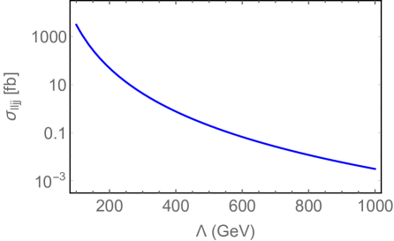
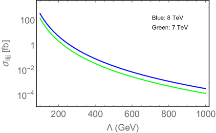
Figure 2: Production cross-section for two same-sign leptons and two jets ($\ell\ell jj$) as a function of $\Lambda$ (GeV) at LHC with $E_{\rm CM}=14$ TeV (left) and $7,\,8$ TeV (right) in green and blue respectively.

The discovery limit, however, depends on the SM background estimate for $\ell\ell jj$ signal, which we discuss below. We will use these results to obtain the current limits on $\Lambda$ derived form the $8~{}\hbox{TeV}$ LHC data, and to derive the expected sensitivity that will be reached when the CM energy is increased to $14~{}\hbox{TeV}$.

   

   

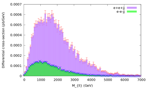
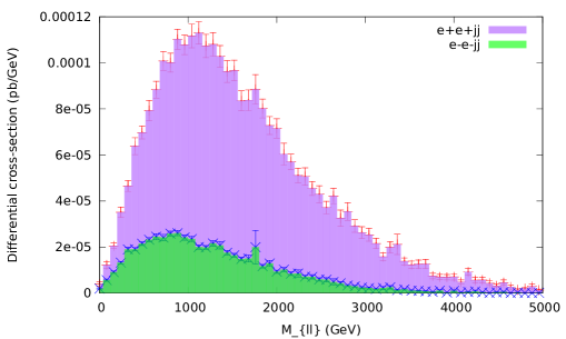
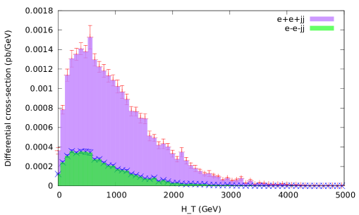
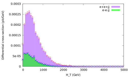
Figure 3: Distributions of the invariant mass of leptons $M_{\ell\ell}$ (top) and transverse mass $H_{T}$ (bottom), for the $\ell\ell jj$ signal events at LHC with $E_{cm}=14$ TeV (left) and $E_{cm}=8$ TeV (right). We took $\Lambda=100~{}\hbox{GeV}$ (see text and Eq.(18)). Subprocesses $\bar{e}\bar{e}jj$ (red dots and lilac histograms) and $eejj$ (blue crosses and green histograms) are shown separately.

IV.1.1 SM background for same-sign dilepton signal at the LHC

The most significant background contribution to our process is generated by SM $t\bar{t}$ production, with marginal contributions from $t\bar{t}W$, $t\bar{t}Z$ and diboson production. For the $t\bar{t}$ background calculation we take $m_{\rm top}=173.34~{}\hbox{GeV}$ topmass and use the Pythia 6.4 Pythia event generator at tree level, which we multiply the by the appropriate $K-$factor  to obtain the NLO+NLL cross-section at the LHC ttbar-7 ; ttbar-8 ; ttbar-14 . This $K$ factor is very significant, for example, the Pythia $t\bar{t}$ production cross-section is $386.8$ pb at $14$ TeV, while, the NNLO prediction is between $805$ and $898$ pb (incorporating the jet energy scale and parton distribution function uncertainties); we use the average value of $851.5$ pb that gives $K=2.2$ factor. For $E_{CM}=8$ TeV, the Pythia prediction is $94$ pb, while the measured value ttbar-8 in the dilepton and lepton+jet channels is $161.9$ pb (there are variations in this number depending not he channel used) so that we use $K=1.7$ in this case.

In our analysis we try to mimic the experimental reconstruction for leptons and jets within Pythia by imposing the following requirements:

• Leptons ($\ell$) are identified as electrons and muons with transverse momentum $p_{T}>$ 10 GeV and rapidity $|\eta|<$2.5. Two leptons with pseudo-rapidities $\eta$ and $\eta+\Delta\eta$, and azimuthal angles $\phi$ and $\phi+\Delta\phi$ will be considered isolated if $\Delta R=\sqrt{(\Delta\eta)^{2}+(\Delta\phi)^{2}}\geq 0.2$. A lepton and a jet will be isolated if $\Delta R\geq 0.4$ and if the $\Delta R\leq 0.2$ cone contains less than $10$ GeV of transverse energy from low-$E_{T}$ hadron activity

• Jets ($j$) are formed with all the final state particles after removing the isolated leptons from the list with PYCELL, a built-in cluster routine within Pythia. The detector is assumed to span the pseudorapidity range $|\eta|\leq 5$ and to be segmented in 100-$\eta$ and 64-$\phi$ bins. The minimum transverse energy $E_{T}$ of each cell is taken as $0.5$ GeV, while we require $E_{T}\geq 2\hbox{GeV}$ for a cell to act as a jet initiator. All the partons within $\Delta R$=0.4 from the jet initiator cell are included in the formation of the jet, and we require $E_{T}\geq 20\hbox{GeV}$ for a cell group to be considered a jet.

We now define the invariant lepton mass $M_{\ell\ell}$ and the transverse event mass $H_{T}$ by

$$M^{2}_{\ell\ell}=2|{\bf p_{1}}||{\bf p_{2}}|\left(1-\cos\theta\right)\,,\qquad H_{T}=\sum_{\ell,j}|{\bf p}_{\perp}|\,,$$ (20)

where $\theta$ is the relative angle of the lepton momenta ${\bf p_{1}}$ and ${\bf p_{2}}$, and we neglected the lepton masses; ${\bf p}_{\perp}$ denotes the corresponding momenta perpendicular to the beam. The $M_{\ell\ell}$ and $H_{T}$ distributions are plotted in Fig. (3) for the signal subprocesses $\bar{e}\bar{e}jj$ (lilac) and $eejj$ (green). We see that the signal distribution from $\bar{e}\bar{e}jj$ peaks at values $M_{\ell\ell}\sim 1-2\hbox{TeV}$ (this property is independent of $\Lambda$), while the SM background is already much suppressed at $M_{\ell\ell}\simeq 2~{}\hbox{TeV}$ (see Fig. (5)). Also from Fig. (3) we find that the corresponding $H_{T}$ distribution for signal events peaks at $500-1000~{}\hbox{GeV}$, while the background is already negligible at $1~{}\hbox{TeV}$ (see Fig. (6)).

The signal events consists of leptons plus jets and do not involve particles like neutrinos that are not detected at the LHC, while the background events that closely mimic the chosen signal, do produce neutrinos which passes through the detector undetected. Therefore, signal events will be characterized by having zero missing transverse to the beam, while any non-zero measurement of the following missing transverse energy

$$E_{\not T}=\left|\sum_{\ell,j}{\bf p}_{\perp}\right|$$ (21)

(where the vector sum is over all visible leptons and jets, and ${\bf p}_{\perp}$ denotes the corresponding momenta perpendicular to the beam) will indicate the presence of particles like neutrinos in the final state, and will correspond to a background event . We will then require $E_{\not T}\leq 15~{}\hbox{GeV}$, in addition to $C1$ in Eq. (19). The usefulness of this cut can be gauged by comparing the cross sections associated with $t\bar{t}$ production listed in table 4: $\sigma_{\ell\ell}$ denotes the dilepton production cross section (two same-sign leptons plus anything); $\sigma_{\ell\ell jj}$ the dilepton plus two jet cross section, when both jets have transverse momentum $p_{T}^{\left(j\right)}\geq 25~{}\hbox{GeV}$; $\sigma_{\ell\ell jj-0}$ the dilepton plus 2 jet cross section  with zero missing energy ($E_{\not T}=0$) and $p_{T}^{\left(j\right)}\geq 25~{}\hbox{GeV}$ and for which we obtain less than one event in our simulations. Finally, $\sigma_{\ell\ell jj-15}$ the dilepton plus 2 jet cross section with missing energy $E_{\not T}\leq 15$ GeVand $p_{T}^{\left(j\right)}\geq~{}25~{}\hbox{GeV}$. We will use these last two quantities to derive a bound on $\Lambda$ (for $E_{CM}=8~{}\hbox{TeV}$), and determine the expected sensitivity for $E_{CM}=14~{}\hbox{TeV}$.

$t\bar{t}$ Production at LHC	$\sigma_{\ell\ell}^{\left(tt\right)}$	$\sigma_{\ell\ell jj}^{\left(tt\right)}$	$\sigma_{\ell\ell jj-0}^{\left(tt\right)}$	$\sigma_{\ell\ell jj-15}^{\left(tt\right)}$
$E_{CM}$=14 TeV	0.47	0.145	$\leq 0.85\times 10^{-3}$	0.0077
$E_{CM}$=8 TeV	0.089	0.0282	$\leq 0.162\times 10^{-3}$	0.001

Table 4: Dominant SM background cross-section from $t\bar{t}$ production (in pb) for same-sign dilepton events at $E_{cm}=14,\,8$ TeV including muons, antimuons, electrons or positron. The fourth (last) column cross sections are obtained requiring $E_{\not T}=0$ ($E_{\not T}\leq 15~{}\hbox{GeV}$); see text. The cross-sections are obtained after multiplying by the appropriate $K$-factor: 2.20 for 14 TeV and 1.7 for 8 TeV.

The missing energy $E_{\not T}$ distribution for the SM background (Fig. (4)) shows that there is a very large number of $\ell\ell jj$ events with $E_{\not T}<100$ GeV, and that this is drastically reduced to a vanishingly small number when the cut $E_{\not T}<15$ GeV is imposed, as also shown in table 4. This clearly indicates that with such a selection criteria, the signal events are retained (as ideally they are characterized by having zero missing energy), while the background can be reduced significantly allowing for a much improved discovery limit. In addition, the invariant lepton mass $M_{\ell\ell}$ (Fig. (5)) and transverse event mass $H_{T}$ (Fig. (6)) distributions show a characteristic difference between signal and background. For example, $M_{\ell\ell}$ distribution for signal (upper panel of Fig. (3)) peaks $M_{\ell\ell}\sim 800$ GeV while the one for background (Fig. (5)) peaks between $M_{\ell\ell}\sim 0-10$ GeV which can be also used for distinguishing between the contributions from new physics and the SM background.

   

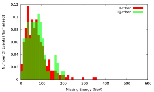
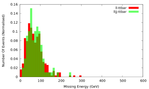
Figure 4: $E_{\not T}$ distribution for $t\bar{t}$ events at the LHC with two leptons (light green) and two leptons and two jets (red); dark green regions correspond to the overlap of the two distributions. Left: $E_{cm}=14$ TeV; right: $E_{cm}=8$ TeV (right).

   

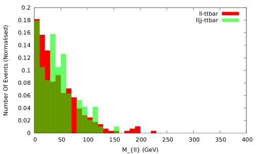
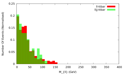
Figure 5: $M_{\ell\ell}$ distribution of the leptons for $t\bar{t}$ events at LHC with $E_{cm}=14$ TeV in left $E_{cm}=8$ TeV in right. The distributions for $\ell\ell$ and $\ell\ell 2j$ events are shown in red and light green respectively (dark green regions correspond to the overlap of the two distributions).

   

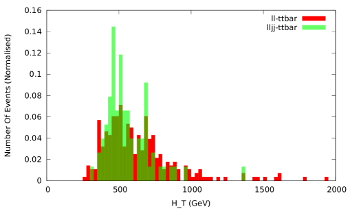
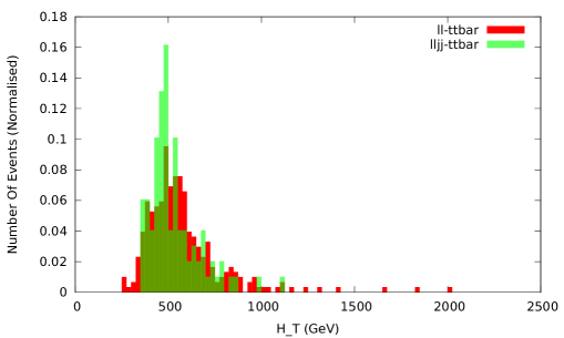
Figure 6: $H_{T}$ for $t\bar{t}$ events at LHC with $E_{cm}=14$ TeV in left $E_{cm}=8$ TeV in right. The distributions for $\ell\ell$ and $\ell\ell 2j$ events are shown in red and light green respectively (dark green regions correspond to the overlap of the two distributions).

IV.2 Bound on $\Lambda$ from LHC data

The LHC has not seen even a 1$\sigma$ excess from the background events so that, assuming Gaussian statistics

$$S/\sqrt{B}\leq 1\,,$$

where $S,\,B$ denote the number of signal and background events respectively. In terms of the luminosity $L$ and the corresponding cross sections $S=\sigma_{\rm signal}L,\,B=\sigma_{\rm back.}L$ where $L$ is integrated luminosity. To date CMS has analyzed LHC data for same sign dileptons for $L=$ 19.5 fb^-1 at $8~{}\hbox{TeV}$ CMS-8TeV ; the background cross-section corresponds to $\sigma_{\rm back.}=\sigma_{\ell\ell jj-15}^{\left(tt\right)}=1$ fb in table 4, we then find

$$\sigma_{\rm signal}\leq 0.224~{}{\rm fb}\,.$$

This in turn puts the bound on the new physics scale: we know $\sigma_{\rm signal}=273$ fb (after cuts) when $\Lambda=100$ GeV (see table 3), and that the signal cross section scales as $1/\Lambda^{6}$ (see Eq. (18)). It follows that

$$\Lambda\geq\left(\frac{273\,{\rm fb}}{0.224\,{\rm fb}}\right)^{1/6}\times 100~{}\hbox{GeV}=327~{}\hbox{GeV}\,.$$ (22)

IV.3 Discovery limit for $\Lambda$ for $\mathcal{O}_{\ell\ell}$ at the LHC

We will follow the same approach to evaluate the discovery limit at the $14~{}\hbox{TeV}$ LHC, requiring now a 3$\sigma$ excess over the background

$$\sigma_{\rm signal}\geq 3\sqrt{\frac{\sigma_{\rm back.}}{L}}\,.$$

From table 4 we find $\sigma_{B}=\sigma^{\left(tt\right)}_{\ell\ell jj-15}=7.7{\rm fb}$ while from table 3 we find $\sigma_{\rm signal}=2590$ fb (after cuts) when the new physics scale $\Lambda=100$ GeV. Using again the simple scaling of the signal cross section with $\Lambda$ (see Eq. (18)) we find

$$\Lambda\leq 382~{}\hbox{GeV}\quad(L=100\,{\rm fb}^{-1},~{}E_{\not T}\leq 15~{}\hbox{GeV})\,,$$ (23)

for an integrated luminosity $L=100$ fb^-1.

If we use a stronger missing energy cut the limit improves. If we require no missing transverse energy then the background cross section drops to $\sigma^{\left(tt\right)}_{\ell\ell jj-0}=\sigma_{\rm back.}=0.85$ fb (see table 4) so that, for the same luminosity,

$$\Lambda\leq 459~{}\hbox{GeV}\quad(L=100\,{\rm fb}^{-1},~{}E_{\not T}=0~{}\hbox{GeV})\,.$$ (24)

IV.4 Hadronically-quiet trilepton at the LHC

   

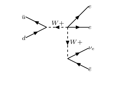
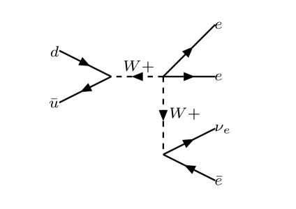
Figure 7: Feynman diagrams generated by the operator ${\cal O}_{\ell\ell}$ and which contribute to the hadronically-quiet trilepton channel $pp\rightarrow ee\bar{e}\nu_{e}$.

The operator $\mathcal{O}_{\ell\ell}$ can also produce hadronically-quiet trilepton events at the LHC, which is sometimes favoured as a signal for new physics because of its clean signature and small SM backgrounds. We find however, that for $\mathcal{O}_{\ell\ell}$ the total signal cross-section is only $3.28$ fb for $\Lambda=$ 100 GeV (see table 5). This small value results from the relatively small branching ratio of the $W$ boson into leptons and the absence of a $t$-channel diagram that generated an important contribution to the $\ell\ell jj$ final state (compare Fig. (7) and Fig. (1)).

$p,p\rightarrow\ell,\ell,\ell,\nu_{\ell}$	$\sigma$ (fb)	$\sigma_{1}$ (fb)	$\sigma_{2}$ (fb)
$p,p\rightarrow\bar{e},\bar{e},e,\bar{\nu_{e}}$	1.2	0.70	0.695
$p,p\rightarrow e,e,\bar{e},\nu_{e}$	0.44	0.39	0.385
Total (including $\mu$)	3.28	2.18	2.16

Table 5: Cross-sections for the hadronically-quiet trilepton signal at the LHC with $E_{cm}=$14 TeV. $\sigma_{1}$ is obtained by imposing the cut $C1$ (cf. Eq. (19)), and $\sigma_{2}$ by imposing both $C1$ and demanding $|M_{e\bar{e}}-M_{z}|>15~{}\hbox{GeV}$.

SM Production at LHC	$\sigma_{\ell\ell\ell}$ (pb)	$\sigma_{\ell\ell\ell-M_{\ell\ell}}$ (pb)	$\sigma_{\ell\ell\ell-M_{\ell\ell}-0}$ (fb)	$\sigma_{\ell\ell\ell-M_{\ell\ell}-15}$ (fb)
$t\bar{t}$	0.99	0.031	$\leq$ 0.85	1.69
$WZ$	0.73	0.171	$\leq$ 0.058	0.46

Table 6: Dominant SM background cross-sections $\sigma_{\ell\ell\ell\ell}$ (in pb) generated by $t\bar{t}$ and $WZ$ production for hadronically-quiet trilepton events at $E_{cm}=14$ TeV including $\mu^{\pm}$ and $e^{\pm}$; the third column provides the numbers when the cut $|M_{\ell\ell}-M_{z}|>15\hbox{GeV}$ is imposed on the events. The cross-sections in the fourth and fifth columns are obtained requiring $E_{\not T}=0$ and $E_{\not T}\leq 15\hbox{GeV}$ respectively (see text for details). The cross-sections are obtained after multiplying by the appropriate $K$-factor (=2.20 for $t\bar{t}$).

$WZ$ production generates a significant background to the process being considered; in order to suppress it we require that the invariant mass $M_{\ell\ell}$ between any opposite-sign leptons of the same flavor satisfies $|M_{\ell\ell}-M_{z}|>15~{}\hbox{GeV}$. Comparing the results in table 5 and table 6 we see that using the cuts we are able to significantly reduce the background compared to the signal cross section of $2.16$ fb for $\Lambda=100~{}\hbox{GeV}$. Following a procedure similar to the one we used in analyzing the same-sign dilepton events and using Eq. (18) we determined the sensitivity to $\Lambda$ using this hadronically-quiet trilepton channel; using a $3\sigma$ limit we obtain,

$$\Lambda\leq 130~{}\hbox{GeV}\quad(E_{\not T}\leq 15~{}\hbox{GeV})\,,\qquad\Lambda\leq 140~{}\hbox{GeV}\quad(E_{\not T}=0~{}\hbox{GeV})\,,$$ (25)

for a luminosity of $100~{}{\rm fb}^{-1}$. As expected from the smaller cross section these limits are weaker than the ones previously obtained.

IV.5 Applicability of the effective field theory

The results above indicate that the reach on new physics scale $\Lambda$ lies in the $\simeq 500~{}\hbox{GeV}$ for the same sign dilepton signature generated by the operator(s) ${\cal O}_{\ell\ell}$ at the LHC with a $14$ TeV CM energy. On the other hand, the dilepton invariant mass distribution (Fig. (3)) peaks at $\sim 1$ TeV, a significantly higher value. We must then investigate whether the effective theory approach is valid in the above processes. Specifically, within the paradigm we have adopted (that of a weakly coupled, renormalization and decoupling heavy physics), we must determine whether this implies that in the reactions under consideration one or more heavy particles carries momentum $\geq\Lambda$ (in which case they could be directly produced and the effective approach would not be applicable). In order to investigate this we display in Fig. (8) the types of heavy physics that could generate at tree level the vertex of interest (containing two charged leptons of the same sign, two $W$ bosons of the same sign and two scalar isodoublets).

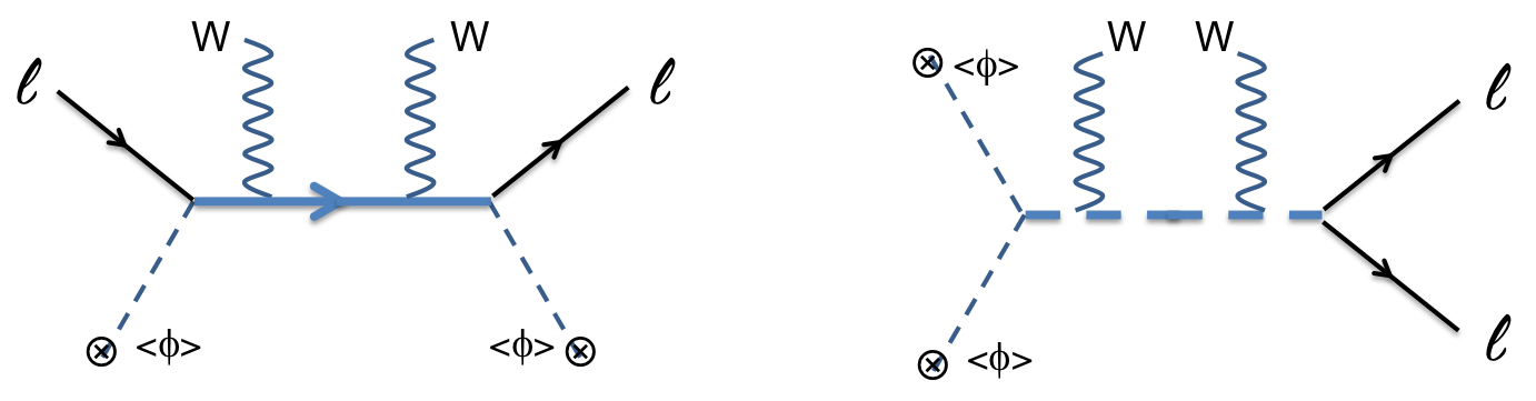
Figure 8: Tree-level graphs that can generate the operators ${\cal O}_{1}$ and ${\cal O}_{3}$ by the exchange of a heavy fermion (left) or scalar (right), both isotriplets with unit hypercharge (denoted by the thick internal lines).

We see from Fig. (8) that there are two possible cases

1. When the heavy particles carry a momentum equal to the invariant dilepton mass, in which case the heavy particle is a boson isotriplet of unit hypercharge; or,

2. When the heavy particles carry a momentum equal to the lepton-$W$ invariant mass, in which case the heavy particle $\Sigma$ will be a heavy fermion isotriplet or isosinglet of zero hypercharge.

The comments above indicate that the effective theory would not be applicable in case 1. The situation for the fermions $\Sigma$ (case 2), however, is different: we see from Fig. 9 that the lepton-$W$ invariant mass peaks at $\lesssim 200~{}\hbox{GeV}$, significantly below the limit on $\Lambda$. It follows that the limits we derive are applicable for the case where the new heavy physics corresponds to the same fermions $\Sigma$ associated with Type III seesaw mechanisms type3 for neutrino mass generation see the appendix A) .

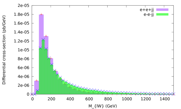
Figure 9: Invariant mass distribution of the lepton with jets at LHC with $E_{cm}=14$ TeV. The red dots (on the lilac histogram) correspond to $\bar{e}\bar{e}jj$ final state; while the blue crosses (on the green histogram) correspond to $eejj$ final state (the green area corresponds to regions where these distributions overlap).

Direct searches of such heavy fermion isotriplets $\Sigma$ (using the full theory) at the $7$ TeV LHC yield a bound $m_{\Sigma}\gtrsim 180~{}\hbox{GeV}$ type3iv , with which our result $\Lambda\gtrsim 300~{}\hbox{GeV}$ compares favourably. In addition, reference CMSdimuon presents an analysis where dimuon + jets data from the 8 TeV LHC are used to derive constraints on heavy Majorana neutrinos that can mix with the muon-neutrino (these correspond to the case where the $\Sigma$ are isosinglets). The results exclude heavy fermion masses in the range $90-500~{}\hbox{GeV}$ provided the mixing is $\geq 0.005$ (for the low mass limit) and $\geq 0.6$ for the higher excluded mass; these constraints are then more stringent than the ones derived above for the case of large mixing. There are also several studies of the discovery potential of Type III seesaw fermions at the $14$ TeV LHC through direct production type3i ; type3ii ; type3iii in lepton-rich final states, and though a comparative signature space analysis of the reach of direct production versus effective theory is beyond the scope of this paper, a benchmark point analysis in type3i suggests that the sensitivity to $\Lambda$ obtained using effective field theory will be competitive to the one derived form direct searches.

V Constraints on PTG operators with right-handed neutrinos

In section III.1 we listed the operators that do not contain right-handed neutrinos and obtained the most stringent bounds on the scale of new physics. In this section we do a similar study for operators that do contain right-handed neutrinos. The list of such operators and their expressions in unitary gauge can be found in Appendix B. Most of these operators contain vertices with 3 fields (see table 7), one of which is a $W,\,Z$ or $H$ boson; the strictest limits on $\Lambda$ are then derived from $Z,W,H$ decays and neutrino magnetic moment, whenever kinematically allowed. When the right-handed neutrinos are too heavy for these decays to occur the limits are weaker, as is the case for the operator $(\overline{\nu^{c}}\nu)|D\phi|^{2}$ that does not contain a three-legged vertex; we comment on this situation at the end of this section.

In the discussion below we will assume that the right-handed neutrinos have a Majorana mass term of the form $\nu_{R}^{T}CM_{\nu}\nu_{R}$ that, for simplicity, we assume to be fully degenerate: $M_{\nu}=m_{\nu}{\mathbbm{1}}$. In cases where the $W,\,Z$ or $H$ decays are allowed, the effects of mixing (generated by Dirac mass terms) will be small delAguila:2008ir and we will ignore them. As in section III.1 the limits on $\Lambda$ obtained below are derived assuming that the operator coefficient is $O(1)$, if this is not the case such limits apply to the scale $\tilde{\Lambda}$ defined in that section; we will also ignore the possibility of cancellations among various effective operator contributions.

V.1 Operators contributing to $Z$-invisible decay

There are two such operators (see table 7):

$$\frac{1}{2}(\overline{\nu^{c}}\gamma^{\mu}N)(i\phi^{\dagger}\stackrel{{\scriptstyle\leftrightarrow}}{{D}}_{\mu}\phi)\supset\frac{v^{3}}{2\sqrt{2}}\overline{\nu^{c}}\not{Z}P_{L}\nu\,,\qquad|\phi|^{2}(\overline{\nu^{c}}\sigma^{\mu\nu}\nu)B_{\mu\nu}\supset-\frac{v^{2}s_{\rm w}}{2}\left(\overline{\nu^{c}}\sigma^{\mu\nu}P_{R}\nu\right)Z_{\mu\nu}\,,$$ (26)

(where $Z_{\mu\nu}=\partial_{\mu}Z_{\nu}-\partial_{\nu}Z_{\mu}$) that generate the following contributions to the invisible $Z$ decay width:

$$\frac{v^{2}m_{\rm z}}{\Lambda^{3}}\overline{\nu^{c}}\not{Z}P_{R}\nu: \Gamma_{Z1}(Z\rightarrow\nu_{R}\nu_{R})=\frac{1}{96\pi}\left(\frac{v^{2}}{\Lambda^{3}}\right)^{2}(m_{\rm z}^{2}-m_{\nu}^{2})\sqrt{m_{\rm z}^{2}-4m_{\nu}^{2}}\,,$$ (27)

$$\frac{vm_{\rm z}}{\Lambda^{3}}(\overline{\nu^{c}}\sigma^{\mu\nu}P_{R}\nu)Z_{\mu\nu}: \Gamma_{Z2}(Z\rightarrow\nu_{R}\nu_{R})=\frac{1}{12\pi}\left(\frac{m_{\rm z}v}{\Lambda^{3}}\right)^{2}\left(m_{\rm z}^{2}+2m_{\nu}^{2}\right)\sqrt{m_{\rm z}^{2}-4m_{\nu}^{2}}\,;$$ (28)

(we made an $O(1)$ change in the operator coefficients in order to have a uniform normalization of the three-legged vertices).

The invisible $Z$-decay width in the standard model is $\Gamma(Z\rightarrow{\rm inv.})=499\pm 1.5$MeV PDG . If the $Z$ decay to right handed neutrinos is kinematically allowed, then, at $3\sigma$, $\Gamma_{Z1,Z2}<4.5$ MeV that gives the contours plotted in Fig. (10). We see from this that the strictest limits on $\Lambda$ are obtained when the right-handed neutrino mass is small:

$$Z1(m_{\nu}\ll m_{\rm z}):~{}\Lambda>354\hbox{GeV}\,,\qquad Z2(m_{\nu}\ll m_{\rm z}):~{}\Lambda>358\hbox{GeV}\,.$$ (29)

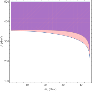
Figure 10: $Z$ invisible decay limit on neutrino mass $m_{\nu}$ versus new physics scale $\Lambda$ plane derived from Eq. (28). The light red region and above is allowed by operator $\overline{\nu^{c}}\not{Z}P_{L}\nu$, and the lilac region is allowed by $(\overline{\nu^{c}}\sigma^{\mu\nu}P_{L,R}\nu)Z_{\mu\nu}$.

V.2 Operators with right-handed neutrinos contributing to $H$-invisible decay

Again referring to table 7 we see that there a single operator of this type:

$$\overline{\nu^{c}}\nu|\phi|^{4}\supset v^{3}H\left(\overline{\nu^{c}}P_{R}\nu\right)\,,$$ (30)

which yields the following invisible decay width

$$\Gamma(H\rightarrow\nu_{R}\nu_{R})=\frac{1}{16\pi}{m_{\rm H}(v/\Lambda)^{6}}\left(1-\frac{2m_{\nu}^{2}}{m_{\rm H}^{2}}\right)\sqrt{1-\frac{4m_{\nu}^{2}}{m_{\rm H}^{2}}}\,.$$ (31)

Using the limit ${\rm Br}(H\rightarrow{\rm inv})<0.3$ invisible_higgs2 , and $\Gamma_{H}^{\rm SM}=4$MeV for the total SM contribution to the $H$ width, we find $\Gamma(H\rightarrow{\rm inv})<1.7\hbox{MeV}$, which we plot in Fig. (11). For light neutrinos this implies,

$$\Lambda>~{}828\hbox{GeV}\,,\quad(m_{\nu}\ll m_{\rm H})\,.$$ (32)

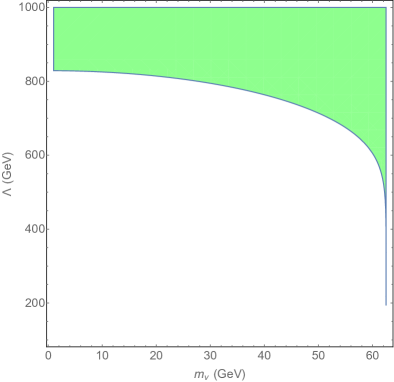
Figure 11: H invisible decay limit on neutrino mass $m_{\nu}$ versus new physics scale $\Lambda$ plane derived from Eq. (31). The shaded region is allowed by operator $\overline{\nu^{c}}\nu|\phi|^{4}$.

V.3 Operators with right-handed neutrinos contributing to $W$-leptonic decay

There are 3 such operators (see table 7):

$$\frac{1}{2}(\overline{\nu^{c}}\gamma^{\mu}E)\left(\phi\epsilon\stackrel{{\scriptstyle\leftrightarrow}}{{D}}_{\mu}\phi\right) \supset -im_{\rm w}v^{2}\overline{\nu^{c}}\not{W}^{+}P_{L}e\,,$$ (33)

$$(\overline{\nu^{c}}\sigma^{\mu\nu}e)(\phi\epsilon\tau^{I}\phi)W^{I}_{\mu\nu} \supset \sqrt{2}v^{2}\left(\partial_{\mu}W_{\nu}^{+}\right)\left(\overline{\nu^{c}}\sigma^{\mu\nu}P_{R}e\right)\,,$$ (34)

$$(\overline{\nu^{c}}D_{\mu}e)(\phi\epsilon D^{\mu}\phi) \supset -i\sqrt{2}\,m_{\rm w}vW^{+}_{\mu}\left(\overline{\nu^{c}}\partial^{\mu}P_{R}e\right)\,,$$ (35)

that leads to three contributions to the leptionic $W$ decay width:

$$\frac{m_{\rm w}v^{2}}{\Lambda^{3}}\overline{\nu^{c}}\not{W}^{+}P_{L}e: \Gamma_{W1}=\frac{1}{192\pi}\left(\frac{v^{4}}{\Lambda^{6}m_{\rm w}^{3}}\right)(m_{\rm w}^{2}-m_{\nu}^{2})^{2}(2m_{\rm w}^{2}+m_{\nu}^{2})\,,$$ (36)

$$\frac{m_{\rm w}v}{\Lambda^{3}}\left(\partial_{\mu}W_{\nu}^{+}\right)\left(\overline{\nu^{c}}\sigma^{\mu\nu}P_{R}e\right): \Gamma_{W2}=\frac{1}{12\pi}\left(\frac{v^{2}}{\Lambda^{6}m_{\rm w}}\right)(m_{\rm w}^{2}-m_{\nu}^{2})^{2}(m_{\rm w}^{2}+2m_{\nu}^{2})\,,$$ (37)

$$\frac{m_{\rm w}v}{\Lambda^{3}}{W^{+}_{\mu}\left(\overline{\nu^{c}}\partial^{\mu}P_{R}e\right)}: \Gamma_{W3}=\frac{1}{192\pi}\left(\frac{v^{2}}{\Lambda^{6}m_{\rm w}^{3}}\right)(m_{\rm w}^{2}-m_{\nu}^{2})^{4}\,.$$ (38)

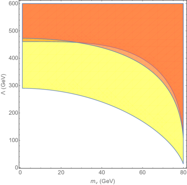
Figure 12: $W$- decay limit on neutrino mass $m_{\nu}$ versus new physics scale $\Lambda$ plane derived form Eq. (38). The yellow region and above is allowed by $W^{+}_{\mu}\left(\overline{\nu^{c}}\partial^{\mu}P_{R}e\right)$, the darker orange region and above is allowed by $(\overline{\nu^{c}}\sigma^{\mu\nu}P_{R}e)\partial_{\mu}W^{+}_{\nu}$, and the orange region and above is allowed by $\overline{\nu^{c}}\not{W}^{+}P_{L}e$.

Now, the branching fraction of $W$ to $\ell+\nu_{\ell}$ (combined leptonic final states) is $\Gamma(W\rightarrow\ell\nu_{\ell})/\Gamma_{W}=(10.86\pm 0.09)\%$ with $\Gamma_{W}=2.085\,\hbox{GeV}$ PDG . This produces the contours of of Fig. (12) in 3$\sigma$ limit; for light neutrinos

$$W1~{}(m_{\nu}\ll m_{\rm w}): \Lambda>473\hbox{GeV}\,,$$ (39)

$$W2~{}(m_{\nu}\ll m_{\rm w}): \Lambda>460\hbox{GeV}\,,$$ (40)

$$W3~{}(m_{\nu}\ll m_{\rm w}): \Lambda>290\hbox{GeV}\,.$$ (41)

V.4 Operators contributing to the neutrino magnetic moment

The operators relevant for this constraint are listed in Eq. (51), for which the most significant constraint is derived from the cooling rate of red-giants and other astrophysical objects plasmon . Using the results in nuSM-5 we find that the strongest restriction is obtained by requiring that the process $\gamma+\nu_{\rm light}\rightarrow\nu_{\rm heavy}$ is not a very efficient cooling mechanism in supernovae plasmon :

$$\Lambda>\left(1-\frac{4m_{\nu}^{2}}{\omega_{P}^{2}}\right)^{1/4}\!\!\times 47\,\hbox{TeV}\,;\quad~{}2m_{\nu}\leq\omega_{P}\simeq 30\,\hbox{MeV}\,,$$ (42)

where $\omega_{P}$ the typical supernova plasma frequency; this same limit is often expressed by the constraint that the $\nu$ magnetic moment is smaller than $3\times 10^{-12}\mu_{B}$.

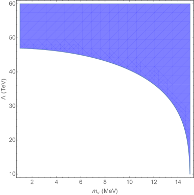
Figure 13: Shaded area: region in the neutrino mass $m_{\nu}$ (GeV) versus new physics scale $\Lambda$ (GeV) plane allowed by the neutrino magnetic moment constraint Eq. (42).

There are no important limits on $\Lambda$ for magnetic coupling for larger neutrino masses; in particular, collider data is useful only when the underlying physics is assumed to be strongly coupled. For weakly-coupled heavy physics the effective operator coefficients are too small to produce a measurable effect given the experimental sensitivity nuSM-5 .

When the above decays are forbidden, or when the operator does not have 3-legged vertices, the experimental constraints are degraded. This is because in this case existing limits are obtained within the context of specific models and cannot be directly extended to limits on all effective operator coefficients. For example, there are strict limits on the masses of the right-handed neutrinos and the right-handed $W_{R}$ gauge bosons present in L-R models Khachatryan:2014dka . But these do not translate to limits on $m_{\nu}$ or $\Lambda$ (when the $W_{R}$ and extra scalars are assumed heavy, with masses $\sim\Lambda$) since the leading effective operators (obtained after integration of these heavy particles) whose effects are strongly constrained by experiment, are not the ones being considered here. The simplest way of seeing this is to note that all our operators violate lepton number, so within such L-R models they will appear multiplied by small coefficients (e.g. by the small vacuum expectation value of a scalar triplet Dhuria:2015cfa ), and have subdominant effects. The point is that without knowledge of the model realized in Nature, one cannot, in general, use limits obtained using some operators to constrain the effects of others. A full analysis of the potential collider reactions that can best probe the operators in table 7 lies beyond the scope of this paper.

VI Conclusions

In this paper we have worked out all possible effective operators of dimension 7 involving SM fields and right-handed neutrinos, indicating those that could be generated at tree generated by the underlying theory and which may then contribute significantly to low energy observables. Our results generalize lists of dimension 7 operators involving only SM fields dim7-1 , as well as earlier earlier partial compilations dim7-2 . All dimension 7 operators violate $B-L$ by two units.

From the operators presented, we selected two that can generate clear dilepton and trilpeton signatures at the LHC. The current limit on the scale of new physics is $\simeq 330~{}\hbox{GeV}$ (Eq. (22)) while the the sensitivity to the scale of new physics can reach $\simeq 460$ GeV (Eq. (24)), with the dilepton channel providing the highest sensitivity. We argue that these results correspond to sensitivity to the presence of heavy fermion triplets (which can also be responsible for type III seesaw mechanism for generating neutrino masses) and are competitive with the ones obtained form direct production. We argued that these limits are not necessarily superseded by the stronger ones derived from precision data given the inability to account for cancellations in the latter.

We have also obtained limits on the NP scale of operators containing right handed neutrinos from $Z,H,W$ decays, which are of the order of $\sim 500~{}{\rm GeV}$ or less for $Z,W$ semi leptonic decays; limits on the $H$ invisible decay gives a stronger limit $\sim 800~{}{\rm GeV}$ (all with a dependence on the right-handed neutrino mass). As for the light neutrinos, much stronger constraints are obtained from the magnetic-moment effective operator, but only for small ($<30~{}\hbox{MeV}$) masses.

Finally, we note that effective Lagrangian models have recently gained interest when studying the LHC sensitivity to various dark matter models; see, for example DM-EFT .

VII Acknowledgements

The work of SB is partially funded by DST-INSPIRE grant no. PHY/P/SUB/01 at IIT Guwahati.

Appendix A Appendix: Loop-generated and potentially tree generated operators

In this appendix we present the arguments for determining whether an operator is necessarily generated by heavy physics loops (LG operators), or if there are types of new physics that can generate the operator at tree-level (potentially tree-generated or PTG operators). As throughout this paper we assume the NP is weakly coupled, and decoupling, and that the full theory is renormalizable. In this case, denoting by $I,~{}E$ the number of internal and external lines respectively, by $L$ the number of loops and by $V_{n}$ the number of vertices with $n$ legs we have the well-known relations

$$L=I-V+1\qquad\sum_{n\geq 3}nV_{n}=2I+E\qquad V=\sum_{n\geq 3}V_{n}$$ (43)

which for tree graphs ($L=0$) in renromaliable theories ($V_{n\geq 5}=0$) imply

$$V_{3}+2V_{4}=E-2$$ (44)

When needed we will denote heavy fermion by $\Psi$ a heavy scalar by $\Phi$ and a a heavy vector by $V$; correspondingly we denote SM vectors, fermions and scalars by $A$, $\psi$ and $\varphi$ respectively.

We will also need some basic properties of the couplings of matter and vector fields in gauge theories. We denote by the index ‘$l$’ a gauge direction associated with a light (SM) vector boson, while an index ‘$h$’ will be associated with the heavy gauge-boson directions. Accordingly the generators are denoted $T^{l}$ and $T^{h}$ and the group structure constants take the generic form $f_{lll,llh,lhh,hhh}$. The group generators in general connect light and heavy particle (fermion and scalar) directions, these we also denote by subindices $l$ and $h$: $(T^{h})_{ll}$, $(T^{h})_{lh}$, $(T^{h})_{hl}$, $(T^{h})_{hh}$ and similarly for $T^{l}$. General properties of gauge theories imply that

$$f_{llh}=0\,,\quad(T^{l})_{lh}=(T^{l})_{hl}=0$$ (45)

Since a vacuum expectation value $\left\langle\Phi\right\rangle$ does not break the electroweak symmetry we also have

$$T^{l}\left\langle\Phi\right\rangle=0\,.$$ (46)

Also, since $T^{h}\left\langle\Phi\right\rangle$ is a vector in the direction of a would-be Goldstone boson, it follows that

$$(T^{h}\left\langle\Phi\right\rangle)_{l}=0$$ (47)

We now use these relations to determine the LG or PTG character of the operators listed in section II.

$\psi^{2}D^{4}$ operators.

These are of the form $\nu^{2}A_{\mu\nu}A_{\rho\sigma},\,\nu^{2}A_{\mu\nu}\tilde{A}_{\rho\sigma}$, and it is straightforward to see that the possible tree diagrams involve a heavy vector, scalar or fermion.

• Heavy fermion exchange: the graphs have a $\nu\Psi A$ vertex and are then proportional to $(T^{l})_{lh}=0$, because of Eq. (45).

• Heavy vector exchange: the graphs have a $AAV$ vertex and are then proportional to $f_{llh}=0$, because of Eq. (45).

• Heavy scalar exchange: the graphs have a $AA\Phi$ vertex, and are then proportional to $\left\langle\Phi\right\rangle\{T^{l},T^{l^{\prime}}\}\Phi^{\prime}=0$, because of Eq. (46).

$\psi^{2}D^{3}\varphi$ operators.

These are of the form $\partial^{\mu}\psi\gamma^{\nu}\varphi\psi A_{\mu\nu}$ or $\partial^{\mu}\psi\gamma^{\nu}\varphi\psi\tilde{A}_{\mu\nu}$ and the possible tree diagrams involve a heavy vector, scalar or fermion.

• Heavy fermion exchange: the graphs have a $\psi\Psi A$ vertex and are then proportional to $(T^{l})_{lh}=0$, because of Eq. (45).

• Heavy vector exchange: the graphs have a $\varphi AV$ vertex and are then proportional to $\left\langle\Phi\right\rangle\{T^{l},T^{h}\}\varphi=0$, because of Eq. (46) and Eq. (47).

• Heavy scalar exchange: the graphs have a $A\varphi\Phi$ vertex, which is proportional to $(T^{l})_{hl}=0$, because of Eq. (45).

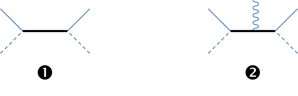
Figure 14: Diagrams that generate operators of the form $\psi^{2}D^{2}\varphi^{2}$ at tree-level (thick lines denote particles with $(\Lambda)$ masses).

$\psi^{2}D^{2}\varphi^{2}$ operators.

These separate in two categories according to whether $D^{2}$ represents a field tensor $D^{2}\rightarrow A_{\mu\nu}$ or not. Both cases can be generated at tree level by the heavy-fermion exchange diagrams ❶ and ❷ in Fig.14. None of the vertices in these graphs are a priori forbidden by the gauge symmetry (though they give rise to mixing among light and heavy fermions and the associated naturality issues).

There are three operators in this group, ${\cal O}_{1,\,3,\,4}$, that are associated with the type I, II and III seesaw neutrino mass generation mechanism. To see this relation explicitly we define

$${\cal O}^{\prime}_{I}=(\ell\phi)\mathchoice{\vbox{\hrule height=0.6pt\hbox{\vrule width=0.6pt,height=5.0pt\kern 5.0pt\vrule width=0.6pt} \hrule height=0.6pt}}{\vbox{\hrule height=0.6pt\hbox{\vrule width=0.6pt,height=5.0pt\kern 5.0pt\vrule width=0.6pt} \hrule height=0.6pt}}{\vbox{\hrule height=0.3pt\hbox{\vrule width=0.3pt,height=2.1pt\kern 2.1pt\vrule width=0.3pt} \hrule height=0.3pt}}{\vbox{\hrule height=0.3pt\hbox{\vrule width=0.3pt,height=1.5pt\kern 1.5pt\vrule width=0.3pt} \hrule height=0.3pt}}(\ell\phi)\,,\quad{\cal O}^{\prime}_{II}=(\ell{\bm{\tau}}\ell)D^{2}(\phi{\bm{\tau}}\phi)\,,\quad{\cal O}^{\prime}_{III}=(\ell{\bm{\tau}}\phi)D^{2}(\ell{\bm{\tau}}\phi)\,,$$ (48)

which can be generated by the exchange of a fermion isosinglet, a scalar isotriplet or a fermion isotriplet, respectively; the relevant graphs are this in Fig. 14. Using the equations of motion (as allowed by the equivalence theorem, see section I) we find that these two set of operators are equivalent:

$$\begin{pmatrix}{\cal O}^{\prime}_{I}\cr{\cal O}^{\prime}_{II}\cr{\cal O}^{\prime}_{III}\end{pmatrix}=\begin{pmatrix}0&0&2\cr 8&4&8\cr-2&0&-6\end{pmatrix}\begin{pmatrix}{\cal O}_{1}\cr{\cal O}_{3}\cr{\cal O}_{4}\end{pmatrix}$$ (49)

The advantage of the primed basis is that it manifestly depicts the type of particles that generate them and nicely matches them to the usual see-saw graphs associated with neutrino mass generation.

Now, ${\cal O}_{1,3}$ contain the term $m_{\rm w}^{2}W^{+}{}^{2}e_{L}^{2}$ (${\cal O}_{2}$ does not), then ${\cal O}^{\prime}_{II,\,III}$ will also have such interactions. The validity of the EFT for ${\cal O}^{\prime}_{II}$ requires the dilepton invariant mass satisfy $M_{\ell\ell}\ll\Lambda$, while for ${\cal O}^{\prime}_{III}$ ihe $W$-lepton should be similarly bound: $M_{\ell W}\ll\Lambda$.

$\psi^{2}D\varphi^{3}$ operators:

contain vertices with 2 fermions and 3 scalars and it is easy to see that can be generated at tree level, for example by $\Psi$ exchange.

$\psi^{2}\varphi^{4}$ operators:

contain vertices with 2 fermions and 4 scalars,. The tree-level graphs then satisfy  $V_{3}+2V_{4}=4$ so that $V_{3}=2,\,V_{4}=1$ or $V_{3}=4$, and the first class of graphs can generate the operators at tree level (vertices: $\psi^{2}\Phi,\,\Phi^{2}\varphi,\,\varphi^{3}\Phi$, and two internal $\Phi$ lines).

Figure 15: Tree-level graph that can generate operators of the form $\psi^{4}D$; lines labeled ‘a’ and ‘b’ correspond to heavy particles (see text for details).

$\psi^{4}D$ operators:

these contain a vertex $\psi^{4}A$, which corresponds to tree-level graphs with $E=5$ and $V_{3}=3,\,V_{4}=0$ ,or $V_{3}=V_{4}=1$, but the latter do not occur since the underlying (renormlizable) theory does not contain 4-legged vertices with fermions; graphs are those in Fig. 15, where

$$\begin{array}[]{c|lllll|ll}{\rm case}&1&2&3&4&5&a&b\cr\hline\cr i&\psi&\psi&A&\psi&\psi&\Phi&\Phi\cr ii&\psi&\psi&A&\psi&\psi&V&V\cr iii&\psi&\psi&A&\psi&\psi&V&\Phi\cr iv&X&\psi&\psi&\psi&\psi&\Psi&V\cr v&X&\psi&\psi&\psi&\psi&\Psi&\Phi\cr\end{array}$$ (50)

• Case $i$ contains the vertex $\Phi\Phi X$ that has a derivative so the operators generated by such graphs are of the form $\psi^{4}X\partial$ and are of dimension 8.

• Case $ii$ contains the vertex $VVA$ with one derivative and also corresponds to operators of dimension 8.

• Case $iii$ contains the vertex $XV\Phi$ of the form which vanish because of Eq. (46) and Eq. (47).

• Cases $iv$ and $v$ require the vertex $\psi X\Psi$ that does not exist because of Eq. (45).

If follows that all these are LG operators.

$\psi^{4}\varphi$ operators:

since 4-fermion interactions can be tree-generated by exchange of a heavy boson, operators of the form $\psi^{4}\varphi$ can be obtained by attaching a $\varphi$ to the internal heavy boson line. These are all PTG operators.

Appendix B Appendix: PTG operators containing right handed neutrinos

The dimension 7 PTG operators containing right-handed neutrinos (see section II) are listed in table 7.

$$\begin{array}[]{ccc}{\cal O}~{}{\rm(see~{}sect~{}\ref{sec:d7_ops})}&\quad{\rm Unitary~{}gauge~{}expression}&\quad{\rm 3-legged~{}vertices~{}in~{}}{\cal O}{\rm~{}(unitary~{}gauge)}\cr\hline\cr\frac{1}{2}(\overline{\nu^{c}}\gamma^{\mu}E)(\phi\epsilon\stackrel{{\scriptstyle\leftrightarrow}}{{D}}_{\mu}\phi)&\quad-\frac{i}{2}g(v+H)^{3}\overline{\nu^{c}}\not{W}^{+}P_{L}e&-im_{\rm w}v^{2}\overline{\nu^{c}}\not{W}^{+}P_{L}e\cr\frac{1}{2}(\overline{\nu^{c}}\gamma^{\mu}N)(i\phi^{\dagger}\stackrel{{\scriptstyle\leftrightarrow}}{{D}}_{\mu}\phi)&\quad\frac{1}{\sqrt{8}}(H+v)^{3}\overline{\nu^{c}}\not{Z}P_{L}\nu&\frac{v^{3}}{2\sqrt{2}}\overline{\nu^{c}}\not{Z}P_{L}\nu\cr(\overline{\nu^{c}}\gamma^{\mu}N)(\partial_{\mu}|\phi|^{2})&\quad-\frac{1}{\sqrt{2}}(H+v)^{2}\partial_{\mu}H\left(\overline{\nu^{c}}\gamma^{\mu}P_{L}\nu\right)&-\frac{v^{2}}{\sqrt{2}}\partial_{\mu}H\left(\overline{\nu^{c}}\gamma^{\mu}P_{L}\nu\right)\cr(\overline{\nu^{c}}\sigma^{\mu\nu}e)(\phi\epsilon\tau^{I}\phi)W^{I}_{\mu\nu}&\quad\sqrt{2}(H+v)^{2}\left[\partial_{\mu}W_{\nu}^{+}-i(eA_{\mu}+gc_{\rm w}Z_{\mu})W_{\nu}^{+}\right]\left(\overline{\nu^{c}}\sigma^{\mu\nu}P_{R}e\right)&\frac{v^{2}}{\sqrt{2}}W_{\mu\nu}^{+}\left(\overline{\nu^{c}}\sigma^{\mu\nu}P_{R}e\right)\cr|\phi|^{2}(\overline{\nu^{c}}\sigma^{\mu\nu}\nu)B_{\mu\nu}&\quad\frac{1}{2}(H+v)^{2}\left(\overline{\nu^{c}}\sigma^{\mu\nu}P_{R}\nu\right)\left(c_{\rm w}F_{\mu\nu}-s_{\rm w}Z_{\mu\nu}\right)&\frac{1}{2}v^{2}\left(\overline{\nu^{c}}\sigma^{\mu\nu}P_{R}\nu\right)\left(c_{\rm w}F_{\mu\nu}-s_{\rm w}Z_{\mu\nu}\right)\cr(\overline{\nu^{c}}D_{\mu}e)(\phi\epsilon D^{\mu}\phi)&\quad\frac{g}{\sqrt{2}}(v+H)^{2}\left[-i\left(\overline{\nu^{c}}\partial^{\mu}P_{R}e\right)W^{+}_{\mu}+\left(\overline{\nu^{c}}P_{R}e\right)W^{+}\cdot(eA-g^{\prime}s_{\rm w}Z)\right]&-i\sqrt{2}\,m_{\rm w}vW^{+}_{\mu}\left(\overline{\nu^{c}}\partial^{\mu}P_{R}e\right)\cr(\overline{\nu^{c}}\nu)|D\phi|^{2}&\quad\frac{1}{2}\left(\overline{\nu^{c}}P_{R}\nu\right)\left\{\left[\partial H+i\frac{m_{\rm z}}{v}(H+v)Z\right]^{2}+\frac{1}{2}g^{2}(v+H)^{2}m_{\rm w}^{2}W^{+}\cdot W^{-}\right\}&--\cr(\overline{\nu^{c}}\nu)|\phi|^{4}&\quad\frac{1}{4}(H+v)^{4}\left(\overline{\nu^{c}}P_{R}\nu\right)&v^{3}H\left(\overline{\nu^{c}}P_{R}\nu\right)\end{array}$$

Table 7: Dimension 7 operators containing right-handed neutrinos, their unitary-gauge expressions, and the vertices with 3 fields that they contain. We defined $F_{\mu\nu}=\partial_{\mu}A_{\nu}-\partial_{\nu}A_{\mu}$, $W^{+}_{\mu\nu}=\partial_{\mu}W^{+}_{\nu}-\partial_{\nu}W^{+}_{\mu}$, and $Z_{\mu\nu}=\partial_{\mu}Z_{\nu}-\partial_{\nu}Z_{\mu}$; $g,\,g^{\prime}$ denote, respectively, the ${SU(2)}_{L}$ and $U(1)_{Y}$ gauge coupling constants.

It follows from this list that there are 8 types of 3-legged vertices involving right-handed neutrinos and contributing to the $Z,H,W$ decays and neutrino magnetic moments:

$$\begin{array}[]{|l|c|c|c|}\hline\cr&{\rm SM-like~{}coupling}&{\rm derivative~{}coupling}&{\rm magnetic~{}coupling}\cr\hline\cr Z&\overline{\nu^{c}}\not{Z}P_{L}\nu&--&\left(\overline{\nu^{c}}\sigma^{\mu\nu}P_{R}\nu\right)Z_{\mu\nu}\cr H&H\left(\overline{\nu^{c}}P_{R}\nu\right)&\partial_{\mu}H\left(\overline{\nu^{c}}\gamma^{\mu}P_{L}\nu\right)&--\cr W&\overline{\nu^{c}}\not{W}^{+}P_{L}e&W^{+}_{\mu}\left(\overline{\nu^{c}}\partial^{\mu}P_{R}e\right)&\left(\overline{\nu^{c}}\sigma^{\mu\nu}P_{R}e\right)W^{+}_{\mu\nu}\cr\gamma&--&--&\left(\overline{\nu^{c}}\sigma^{\mu\nu}P_{R}\nu\right)F_{\mu\nu}\cr\hline\cr\end{array}$$ (51)

The most significant constraints on $\Lambda$ derived from these vertices were derived in section V.

References

- (1) See for example, M. C. Gonzalez-Garcia and Y. Nir, “Neutrino masses and mixing: Evidence and implications,” Rev. Mod. Phys. 75, 345 (2003) [hep-ph/0202058]; R. Mohapatra, S. Antusch, K. Babu, G. Barenboim, M.-C. Chen, et al., ”Theory of neutrinos: A White paper,” Rept. Prog. Phys. 70, 1757 (2007), [arXiv:hep-ph/0510213].
- (2) See for example, G. Bertone, D. Hooper and J. Silk, “Particle dark matter: Evidence, candidates and constraints,” Phys. Rept. 405, 279 (2005) [hep-ph/0404175].
- (3) See for example, J. Polchinski, “Effective field theory and the Fermi surface,” In *Boulder 1992, Proceedings, Recent directions in particle theory* 235-274, and Calif. Univ. Santa Barbara - NSF-ITP-92-132 (92,rec.Nov.) 39 p. (220633) Texas Univ. Austin - UTTG-92-20 (92,rec.Nov.) 39 p [hep-th/9210046].
- (4) K. G. Wilson and J. B. Kogut, “The Renormalization group and the epsilon expansion,” Phys. Rept. 12, 75 (1974).
- (5) S. Weinberg, “Phenomenological Lagrangians,” Physica A 96 (1979) 327; For a pedagogical review see: A. Dobado, A. Gomez-Nicola, A. L. Maroto and J. R. Pelaez, Effective Lagrangians for the Standard Model (Spinger, 1997; ISBN-10: 3540625704, ISBN-13: 978-3540625704)
- (6) H. Georgi, “On-shell effective field theory,” Nucl. Phys. B 361 (1991) 339; J. Wudka, “Electroweak effective Lagrangians,” Int. J. Mod. Phys. A 9, 2301 (1994) [hep-ph/9406205]; C. Arzt, “Reduced effective Lagrangians,” Phys. Lett. B 342, 189 (1995) [hep-ph/9304230].
- (7) G. ’t Hooft and M. J. G. Veltman, “Regularization and Renormalization of Gauge Fields,” Nucl. Phys. B 44, 189 (1972).
- (8) T. Appelquist and J. Carazzone, “Infrared Singularities and Massive Fields,” Phys. Rev. D 11 (1975) 2856. For a pedagogical introduction see: J. Collins, Renormalization: An Introduction to Renormalization, the Renormalization Group and the Operator-Product Expansion (Cambridge University Press, 1986; ISBN-10: 0521311772, ISBN-13: 978-0521311779).
- (9) G. C. Branco, P. M. Ferreira, L. Lavoura, M. N. Rebelo, M. Sher and J. P. Silva, “Theory and phenomenology of two-Higgs-doublet models,” Phys. Rept. 516, 1 (2012) [arXiv:1106.0034 [hep-ph]].
- (10) K. Agashe, R. Contino and A. Pomarol, “The Minimal composite Higgs model,” Nucl. Phys. B 719 (2005) 165 [hep-ph/0412089].
- (11) M. J. G. Veltman, “The Infrared - Ultraviolet Connection,” Acta Phys. Polon. B 12 (1981) 437.
- (12) S. Weinberg, “Baryon and Lepton Nonconserving Processes,” Phys. Rev. Lett. 43, 1566 (1979).
- (13) W. Buchmuller and D. Wyler, “Effective Lagrangian Analysis of New Interactions and Flavor Conservation,” Nucl. Phys. B 268, 621 (1986).
- (14) B. Grzadkowski, M. Iskrzynski, M. Misiak and J. Rosiek, “Dimension-Six Terms in the Standard Model Lagrangian,” JHEP 1010, 085 (2010) [arXiv:1008.4884 [hep-ph]].
- (15) L. Lehman, “Extending the Standard Model Effective Field Theory with the Complete Set of Dimension-7 Operators,” Phys. Rev. D 90, no. 12, 125023 (2014) [arXiv:1410.4193 [hep-ph]].
- (16) K. S. Babu and C. N. Leung, “Classification of effective neutrino mass operators,” Nucl. Phys. B 619, 667 (2001) [hep-ph/0106054]; A. de Gouvea and J. Jenkins, “A Survey of Lepton Number Violation Via Effective Operators,” Phys. Rev. D 77, 013008 (2008) [arXiv:0708.1344 [hep-ph]]; F. Bonnet, D. Hernandez, T. Ota and W. Winter, “Neutrino masses from higher than d=5 effective operators,” JHEP 0910, 076 (2009) [arXiv:0907.3143 [hep-ph]]; P. W. Angel, N. L. Rodd and R. R. Volkas, “Origin of neutrino masses at the LHC: effective operators and their ultraviolet completions,” Phys. Rev. D 87, no. 7, 073007 (2013) [arXiv:1212.6111 [hep-ph]]; C. Degrande, “A basis of dimension-eight operators for anomalous neutral triple gauge boson interactions,” JHEP 1402, 101 (2014) [arXiv:1308.6323 [hep-ph]].
- (17) S. Weinberg, “Varieties of Baryon and Lepton Nonconservation,” Phys. Rev. D 22, 1694 (1980); K. S. Babu and R. N. Mohapatra, “B-L Violating Proton Decay Modes and New Baryogenesis Scenario in SO(10),” Phys. Rev. Lett. 109, 091803 (2012) [arXiv:1207.5771 [hep-ph]]; K. S. Babu and R. N. Mohapatra, “B-L Violating Nucleon Decay and GUT Scale Baryogenesis in SO(10),” Phys. Rev. D 86, 035018 (2012) [arXiv:1203.5544 [hep-ph]]; G. Chalons and F. Domingo, “Dimension 7 operators in the b to s transition,” Phys. Rev. D 89, no. 3, 034004 (2014) [arXiv:1303.6515 [hep-ph]].
- (18) H. A. Weldon and A. Zee, “Operator Analysis of New Physics,” Nucl. Phys. B 173, 269 (1980); C. Arzt, M. B. Einhorn and J. Wudka, “Effective Lagrangian approach to precision measurements: The Anomalous magnetic moment of the muon,” Phys. Rev. D 49, 1370 (1994) [hep-ph/9304206]. S. Bar-Shalom, A. Soni and J. Wudka, “EFT naturalness: an effective field theory analysis of Higgs naturalness,” arXiv:1405.2924 [hep-ph]; S. Dawson, I. M. Lewis and M. Zeng, “Effective field theory for Higgs boson plus jet production,” Phys. Rev. D 90, no. 9, 093007 (2014) [arXiv:1409.6299 [hep-ph]]; R. Catena, “Prospects for direct detection of dark matter in an effective theory approach,” JCAP 1407, 055 (2014) [arXiv:1406.0524 [hep-ph]]; S. Matsumoto, S. Mukhopadhyay and Y. L. S. Tsai, “Singlet Majorana fermion dark matter: a comprehensive analysis in effective field theory,” JHEP 1410, 155 (2014) [arXiv:1407.1859 [hep-ph]]; G. M. Pruna and A. Signer, “The decay in a systematic effective field theory approach with dimension 6 operators,” JHEP 1410, 14 (2014) [arXiv:1408.3565 [hep-ph]]; A. Biek tter, A. Knochel, M. Kr mer, D. Liu and F. Riva, “Vices and virtues of Higgs effective field theories at large energy,” Phys. Rev. D 91, 055029 (2015) [arXiv:1406.7320 [hep-ph]]; M. Duch, B. Grzadkowski and J. Wudka, “Classification of effective operators for interactions between the Standard Model and dark matter,” JHEP 1505, 116 (2015) [arXiv:1412.0520 [hep-ph]].
- (19) See for example, A. Zee, Phys. Lett. B 93, 389 (1980) Erratum: [Phys. Lett. B 95, 461 (1980)].
- (20) A. Aparici, K. Kim, A. Santamaria and J. Wudka, “Right-handed neutrino magnetic moments,” Phys. Rev. D 80, 013010 (2009) [arXiv:0904.3244 [hep-ph]].
- (21) F. del Aguila, S. Bar-Shalom, A. Soni and J. Wudka, “Heavy Majorana Neutrinos in the Effective Lagrangian Description: Application to Hadron Colliders,” Phys. Lett. B 670 (2009) 399 [arXiv:0806.0876 [hep-ph]].
- (22) See for example, J. D. Vergados, “The Neutrinoless double beta decay from a modern perspective,” Phys. Rept. 361, 1 (2002) [hep-ph/0209347]; F. del Aguila, A. Aparici, S. Bhattacharya, A. Santamaria and J. Wudka, “Effective Lagrangian approach to neutrinoless double beta decay and neutrino masses,” JHEP 1206 (2012) 146 [arXiv:1204.5986 [hep-ph]].
- (23) See for example, M. Spira, A. Djouadi, D. Graudenz and P. M. Zerwas, “Higgs boson production at the LHC,” Nucl. Phys. B 453, 17 (1995) [hep-ph/9504378]. M. B. Einhorn and J. Wudka, Nucl. Phys. B 877 (2013) 792 [arXiv:1308.2255 [hep-ph]].
- (24) C. Arzt, M. B. Einhorn and J. Wudka, “Patterns of deviation from the standard model,” Nucl. Phys. B 433, 41 (1995) [hep-ph/9405214].
- (25) M. B. Einhorn and J. Wudka, “The Bases of Effective Field Theories,” Nucl. Phys. B 876, 556 (2013) [arXiv:1307.0478 [hep-ph]].
- (26) A. de Gouvea, J. Herrero-Garcia and A. Kobach, “Neutrino Masses, Grand Unification, and Baryon Number Violation,” Phys. Rev. D 90, no. 1, 016011 (2014) [arXiv:1404.4057 [hep-ph]].
- (27) J. D. Vergados, H. Ejiri and F. Simkovic, Rept. Prog. Phys. 75 (2012) 106301 doi:10.1088/0034-4885/75/10/106301 [arXiv:1205.0649 [hep-ph]].
- (28) See F. del Aguila, A. Aparici, S. Bhattacharya, A. Santamaria and J. Wudka, JHEP 1206 (2012) 146 doi:10.1007/JHEP06(2012)146 [arXiv:1204.5986 [hep-ph]], and references therein.
- (29) K.A. Olive et al. (Particle Data Group), Chin. Phys. C, 38, 090001 (2014).
- (30) V. Castellani and S. Degl’Innocenti, Astrophys. J. 402 (1993) 574. M. Catelan, J. A. d. F. Pacheco and J. E. Horvath, Astrophys. J. 461 (1996) 231 [astro-ph/9509062]. M. Haft, G. Raffelt and A. Weiss, Astrophys. J. 425 (1994) 222 [Astrophys. J. 438 (1995) 1017] [astro-ph/9309014]. G. G. Raffelt, Astrophys. J. 365 (1990) 559. G. G. Raffelt, Phys. Rev. Lett. 64 (1990) 2856. G. Raffelt and A. Weiss, Astron. Astrophys. 264 (1992) 536. A. Heger, A. Friedland, M. Giannotti and V. Cirigliano, Astrophys. J. 696 (2009) 608 [arXiv:0809.4703 [astro-ph]].A. Heger, A. Friedland, M. Giannotti and V. Cirigliano, Astrophys. J. 696 (2009) 608 [arXiv:0809.4703 [astro-ph]]. G. Raffelt, Stars as Laboratories for Fundamental Physics: The Astrophysics of Neutrinos, Axions, and Other Weakly Interacting Particles, (U. Chicago Press, 1996; ISBN-10: 0226702723, ISBN-13: 978-0226702728) N. Iwamoto, L. Qin, M. Fukugita and S. Tsuruta, Phys. Rev. D 51 (1995) 348. G. G. Raffelt, Phys. Rept. 320 (1999) 319.
- (31) F. del Aguila, A. Aparici, S. Bhattacharya, A. Santamaria and J. Wudka, JHEP 1205 (2012) 133 doi:10.1007/JHEP05(2012)133 [arXiv:1111.6960 [hep-ph]].
- (32) A. Belyaev, N. D. Christensen and A. Pukhov, “CalcHEP 3.4 for collider physics within and beyond the Standard Model,” Comput. Phys. Commun. 184 (2013) 1729 [arXiv:1207.6082 [hep-ph]].
- (33) H. L. Lai et al. [CTEQ Collaboration], “Global QCD analysis of parton structure of the nucleon: CTEQ5 parton distributions,” Eur. Phys. J. C 12, 375 (2000) [arXiv:hep-ph/9903282].
- (34) [ATLAS Collaboration], “Physics at a High-Luminosity LHC with ATLAS,” arXiv:1307.7292 [hep-ex].
- (35) J. Varela [CMS Collaboration], “Prospects for physics at high luminosity with CMS,” EPJ Web Conf. 49, 11003 (2013).
- (36) ATLAS Collaboration, ‘Physics at a High-Luminosity LHC with ATLAS’, ATL-PHYS-PUB-2012-001, https://cds.cern.ch/record/1472518.
- (37) The ATLAS, CDF, CMS and D0 Collaborations, First combination of Tevatron and LHC measurements of the top-quark mass; arXiv:1403.4427 [hep-ex].
- (38) T. Sjostrand, S. Mrenna and P. Skands, “PYTHIA 6.4 physics and manual,” JHEP 0605, 026 (2006) [arXiv:hep-ph/0603175].
- (39) V. Khachatryan et al. [CMS Collaboration], “First Measurement of the Cross Section for Top-Quark Pair Production in Proton-Proton Collisions at TeV,” Phys. Lett. B 695 (2011) 424 [arXiv:1010.5994 [hep-ex]].
- (40) A. Calderon [ATLAS and CMS Collaborations], “Top pair cross section measurements at the LHC,” arXiv:1301.1158 [hep-ex].
- (41) S. Moch and P. Uwer, “Theoretical status and prospects for top-quark pair production at hadron colliders,” Phys. Rev. D 78 (2008) 034003 [arXiv:0804.1476 [hep-ph]].
- (42) S. Chatrchyan et al. [CMS Collaboration], “Search for new physics in events with same-sign dileptons and jets in pp collisions at = 8 TeV,” JHEP 1401 (2014) 163 [arXiv:1311.6736, arXiv:1311.6736 [hep-ex]].
- (43) R. Foot, H. Lew, X. G. He and G. C. Joshi, “Seesaw Neutrino Masses Induced by a Triplet of Leptons,” Z. Phys. C 44, 441 (1989).
- (44) CMS Physics Analysis Summary, CMS PAS EXO-11-073.
- (45) V. Khachatryan et al. [CMS Collaboration], “Search for heavy Majorana neutrinos in jets events in proton-proton collisions at = 8 TeV,” Phys. Lett. B 748, 144 (2015) doi:10.1016/j.physletb.2015.06.070 [arXiv:1501.05566 [hep-ex]].
- (46) F. del Aguila and J. A. Aguilar-Saavedra, ‘Distinguishing seesaw models at LHC with multi-lepton signals,” Nucl. Phys. B 813, 22 (2009) [arXiv:0808.2468 [hep-ph]].
- (47) R. Franceschini, T. Hambye and A. Strumia, “Type-III see-saw at LHC,” Phys. Rev. D 78, 033002 (2008) [arXiv:0805.1613 [hep-ph]].
- (48) B. Bajc and G. Senjanovic, “Seesaw at LHC,” JHEP 0708, 014 (2007) [hep-ph/0612029].
- (49) See, for example: F. del Aguila, S. Bar-Shalom, A. Soni and J. Wudka, Phys. Lett. B 670 (2009) 399 doi:10.1016/j.physletb.2008.11.031 [arXiv:0806.0876 [hep-ph]].
- (50) V. Khachatryan et al. [CMS Collaboration], Eur. Phys. J. C 74 (2014) 11, 3149 doi:10.1140/epjc/s10052-014-3149-z [arXiv:1407.3683 [hep-ex]].
- (51) M. Dhuria, C. Hati, R. Rangarajan and U. Sarkar, Phys. Rev. D 92 (2015) 3, 031701 doi:10.1103/PhysRevD.92.031701 [arXiv:1503.07198 [hep-ph]].
- (52) G. Aad et al. [ATLAS Collaboration], JHEP 1601, 172 (2016) doi:10.1007/JHEP01(2016)172 [arXiv:1508.07869 [hep-ex]].
- (53) J. Goodman, M. Ibe, A. Rajaraman, W. Shepherd, T. M. P. Tait and H. B. Yu, “Constraints on Dark Matter from Colliders,” Phys. Rev. D 82, 116010 (2010) [arXiv:1008.1783 [hep-ph]]; G. Busoni, A. De Simone, J. Gramling, E. Morgante and A. Riotto, “On the Validity of the Effective Field Theory for Dark Matter Searches at the LHC, Part II: Complete Analysis for the -channel,” JCAP 1406, 060 (2014) [arXiv:1402.1275 [hep-ph]]; G. Busoni, A. De Simone, T. Jacques, E. Morgante and A. Riotto, “On the Validity of the Effective Field Theory for Dark Matter Searches at the LHC Part III: Analysis for the -channel,” JCAP 1409, 022 (2014) [arXiv:1405.3101 [hep-ph]]; J. Abdallah, A. Ashkenazi, A. Boveia, G. Busoni, A. De Simone, C. Doglioni, A. Efrati and E. Etzion et al., “Simplified Models for Dark Matter and Missing Energy Searches at the LHC,” arXiv:1409.2893 [hep-ph].