Internal circle uplifts, transversality and stratified G-structures

Abstract

We study stratified G-structures in $\mathcal{N}=2$ compactifications of M-theory on eight-manifolds $M$ using the uplift to the auxiliary nine-manifold ${\hat{M}}=M\times S^{1}$. We show that the cosmooth generalized distribution $\hat{\mathcal{D}}$ on ${\hat{M}}$ which arises in this formalism may have pointwise transverse or non-transverse intersection with the pull-back of the tangent bundle of $M$, a fact which is responsible for the subtle relation between the spinor stabilizers arising on $M$ and ${\hat{M}}$ and for the complicated stratified G-structure on $M$ which we uncovered in previous work. We give a direct explanation of the latter in terms of the former and relate explicitly the defining forms of the $\mathrm{SU}(2)$ structure which exists on the generic locus $\mathcal{U}$ of $M$ to the defining forms of the $\mathrm{SU}(3)$ structure which exists on an open subset $\hat{\mathcal{U}}$ of ${\hat{M}}$, thus providing a dictionary between the eight- and nine-dimensional formalisms.

Introduction

General $\mathcal{N}=2$ flux compactifications of eleven-dimensional supergravity sugra11 on eight-manifolds $M$ have two independent internal supersymmetry generators $\xi_{1},\xi_{2}$ which are global sections of the rank sixteen bundle $S$ of Majorana spinors on $M$. The class of such compactifications is little explored, with the notable exception of compactifications down to Minkowski 3-space BeckerCY , which arise when imposing the Weyl condition on $\xi_{1}$ and $\xi_{2}$ and which, as a consequence of no-go theorems, can only support a flux at the quantum, rather than classical, level. Relaxing this condition leads to backgrounds which can support classical fluxes and which have a surprisingly rich geometry. Some aspects of such backgrounds were discussed in Palti using a formalism which uses the auxiliary nine-manifold ${\hat{M}}\stackrel{{\scriptstyle{\rm def.}}}{{=}}M\times S^{1}$ and the canonical lifts ${\hat{\xi}}_{1},{\hat{\xi}}_{2}$ to ${\hat{M}}$ of the internal supersymmetry generators (see also ga2 ). In that approach, one finds that ${\hat{M}}$ is endowed with a stratified G-structure whose strata are defined by the isomorphism type of the stabilizer group inside ($\mathrm{Spin}(9)$) of the pair of lifted spinors at various points of ${\hat{M}}$. The strata of ${\hat{M}}$ correspond Palti to stabilizers isomorphic with $\mathrm{SU}(3)$, $\mathrm{G_{2}}$ or $\mathrm{SU}(4)$. On the other hand, it was shown in msing that the stabilizer stratification induced by $\xi_{1}$ and $\xi_{2}$ on $M$ has $\mathrm{SU}(2)$, $\mathrm{SU}(3)$, $\mathrm{G_{2}}$ and $\mathrm{SU}(4)$ strata, whose description is considerably more complex. This stratification of $M$ coincides with a certain coarsening of the preimage of the connected refinement of the canonical Whitney stratification Whitney ; Gibson of a four-dimensional compact semi-algebraic BCR ; BPR body $\mathfrak{P}\subset\mathbb{R}^{4}$ through a certain map $B:M\rightarrow\mathbb{R}^{4}$ whose image is contained in $\mathfrak{P}$. As shown in msing , this complicated stratification generalizes what happens in the much simpler case of $\mathcal{N}=1$ M-theory flux compactifications on eight-manifolds MartelliSparks ; Tsimpis ; g2 ; g2s (which extend the classically fluxless case of Becker1 ; Becker2 ; Constantin ), where the relevant semi-algebraic body is the interval $[-1,1]$, endowed with its Whitney stratification.

The complexity of the picture found in msing may come as a surprise given the relative simplicity of the stabilizer stratification of ${\hat{M}}$. The purpose of this note is to explain this difference. Embedding $M$ into ${\hat{M}}$ as a hypersurface $j(M)$ located at some fixed point of $S^{1}$, we show that the cosmooth Drager generalized distribution Freeman ; BulloLewis ; Michor ; Ratiu $\mathcal{D}$ of msing (which is the polar distribution defined by three 1-forms $V_{1},V_{2},V_{3}\in\Omega^{1}(M)$) coincides with the intersection of $TM$ with the restriction $j^{\ast}(\hat{\mathcal{D}})\equiv\hat{\mathcal{D}}|_{j(M)}$ of the polar distribution $\hat{\mathcal{D}}$ which is defined on ${\hat{M}}$ by three 1-forms ${\hat{V}}_{1},{\hat{V}}_{2},{\hat{V}}_{3}\in\Omega^{1}({\hat{M}})$. The latter can be expressed as bilinears in ${\hat{\xi}}_{1}$ and ${\hat{\xi}}_{2}$. The algebraic constraints satisfied by $V_{1},V_{2}$ and $V_{3}$ as a result of Fierz identities for $\xi_{1}$ and $\xi_{2}$ are equivalent with the algebraic constraints satisfied by ${\hat{V}}_{1},{\hat{V}}_{2}$ and ${\hat{V}}_{3}$ as a result of Fierz identities for ${\hat{\xi}}_{1}$ and ${\hat{\xi}}_{2}$. The intersection $\mathcal{D}=j^{\ast}(\hat{\mathcal{D}})\cap TM$ may be pointwise transverse or non-transverse, giving rise to a disjoint union decomposition $M=\mathcal{T}\sqcup\mathcal{N}$, where $\mathcal{T}$ is the transverse locus and $\mathcal{N}$ is the non-transverse locus of $M$. While $\mathcal{D}$ and $j^{\ast}(\hat{\mathcal{D}})$ coincide when restricted to $\mathcal{N}$, the ranks of their restrictions to $\mathcal{T}$ differ by one. The fact that $\mathcal{T}$ may be nonempty turns out to be responsible for the difference between the stabilizer stratifications of $M$ and ${\hat{M}}$ and explains the increased complexity of the former when compared to the latter. In the special case when the transverse locus is empty (which turns out to be the case considered in Palti ), the equality $\mathcal{D}=j^{\ast}(\hat{\mathcal{D}})$ holds globally on $M$ and the stabilizer stratification of $M$ is obtained directly from that of ${\hat{M}}$ by intersecting every stratum of the latter with $j(M)$. In the generic case when $\mathcal{T}\neq\emptyset$, the relation between the stabilizer stratifications of $M$ and ${\hat{M}}$ can be understood using a version of known facts FinoTomassini ; ChiossiSalamon ; CabreraSU3 ; Knotes ; ContiSalamon ; Bedulli regarding G-structures induced on orientable hypersurfaces of a G-structured manifold. On the open stratum $\mathcal{U}\subset M$ which carries an $\mathrm{SU}(2)$ structure (the “generic locus” of msing ), this observation allows one to give an explicit formula for the defining forms of the $\mathrm{SU}(2)$ structure in terms of the defining forms of the $\mathrm{SU}(3)$ structure which exists Palti on an open subset $\hat{\mathcal{U}}$ of ${\hat{M}}$.

The note is organized as follows. Section 1 briefly recalls some results of msing , to which we refer the reader for further information. Section 2 discusses the stabilizer stratification of ${\hat{M}}$ and compares its intersection with $j(M)$ with the $B$-preimage of the connected refinement of the canonical Whitney stratification of $\mathfrak{P}$. Section 3 takes up the issue of transversality of the pointwise intersection of $j^{\ast}(\hat{\mathcal{D}})$ with $TM$ and shows how the transverse or non-transverse character of this intersection explains the increased complexity of the stabilizer stratification of $M$ as compared to that of ${\hat{M}}$. The same section shows how the stratified G-structure of $M$ can be obtained by reducing that of ${\hat{M}}$ along this intersection. Section 4 expresses the defining form of the $\mathrm{SU}(2)$ structure which exists on the generic locus of $M$ in terms of the defining forms of the $\mathrm{SU}(3)$ structure which exists on an open subset of ${\hat{M}}$, while Section 5 concludes.

Notations and conventions.

We use the same notations and conventions as reference msing , to which we refer the reader for details. An equality which holds for any point of a subset $A$ of a manifold is written as $=_{A}$.

1 Brief summary of the eight-dimensional formalism

Let $S$ denote the rank 16 vector bundle of Majorana spinors on $M$ (which is endowed with the admissible AC1 ; AC2 scalar product $\Scr B$) and $\nu$ denote the volume form of $(M,g)$. Let $\gamma:\wedge T^{\ast}M\rightarrow\mathrm{End}(S)$ be the structure morphism of $S$. Given two Majorana spinors $\xi_{1},\xi_{2}\in\Gamma(M,S)$ which are $\Scr B$-orthonormal everywhere, we define the 0- and 1-forms:

$$b_{i}=\Scr B(\xi_{i},\gamma(\nu)\xi_{i})~{},~{}b_{3}\stackrel{{\scriptstyle{\rm def.}}}{{=}}\Scr B(\xi_{1},\gamma(\nu)\xi_{2})~{}$$ (1)

$$V_{i}=_{U}\Scr B(\xi_{i},\gamma_{a}\xi_{i})e^{a}~{},~{}V_{3}\stackrel{{\scriptstyle{\rm def.}}}{{=}}\Scr B(\xi_{1},\gamma_{a}\xi_{2})e^{a}~{}~{},~{}~{}W\stackrel{{\scriptstyle{\rm def.}}}{{=}}_{U}\Scr B(\xi_{1},\gamma_{a}\gamma(\nu)\xi_{2})e^{a}$$

with $i=1,2$ and the linear combinations:

$$b_{\pm}\stackrel{{\scriptstyle{\rm def.}}}{{=}}\frac{1}{2}(b_{1}\pm b_{2})~{},~{}V_{\pm}\stackrel{{\scriptstyle{\rm def.}}}{{=}}\frac{1}{2}(V_{1}\pm V_{2})~{}.$$ (2)

It is convenient to consider the smooth map:

$$b\stackrel{{\scriptstyle{\rm def.}}}{{=}}(b_{+},b_{-},b_{3}):M\rightarrow\mathbb{R}^{3}~{}~{}.$$

The Fierz identities for $\xi_{1},\xi_{2}$ imply msing that (1) satisfy the constraints:

$$\begin{split}&||V_{-}||^{2}+b_{-}^{2}=||V_{3}||^{2}+b_{3}^{2}~{}~{},~{}~{}||V_{+}||^{2}+b_{+}^{2}=1-(||V_{3}||^{2}+b_{3}^{2})\\ &\langle V_{+},V_{-}\rangle+b_{+}b_{-}=\langle V_{+},V_{3}\rangle+b_{+}b_{3}=\langle V_{-},V_{3}\rangle+b_{-}b_{3}=0~{}~{}\\ &||W||^{2}+||V_{3}||^{2}=1+b_{-}^{2}-b_{+}^{2}~{}\\ &\langle W,V_{+}\rangle=0~{}~{},~{}~{}\langle W,V_{-}\rangle=b_{3}~{}~{},~{}~{}\langle W,V_{3}\rangle=-b_{-}~{}~{}.\end{split}$$ (3)

In view of the first two relations, we define:

$$\beta\stackrel{{\scriptstyle{\rm def.}}}{{=}}\sqrt{||V_{-}||^{2}+b_{-}^{2}}=\sqrt{||V_{3}||^{2}+b_{3}^{2}}=\sqrt{1-b_{+}^{2}-||V_{+}||^{2}}:M\rightarrow\mathbb{R}~{}~{}.$$ (4)

Consider the cosmooth generalized distributions:

$$\mathcal{D}\stackrel{{\scriptstyle{\rm def.}}}{{=}}\ker V_{+}\cap\ker V_{-}\cap\ker V_{3}\subset TM~{}~{},~{}~{}\mathcal{D}_{0}\stackrel{{\scriptstyle{\rm def.}}}{{=}}\mathcal{D}\cap\ker W\subset\mathcal{D}~{}~{}.$$ (5)

As shown in msing , the rank stratifications of $M$ induced by $\mathcal{D}$ and $\mathcal{D}_{0}$ have the same open stratum, the so-called generic locus of $M$:

$$\mathcal{U}\stackrel{{\scriptstyle{\rm def.}}}{{=}}\{p\in M|{\rm rk}\mathcal{D}(p)=5\}=\{p\in M|{\rm rk}\mathcal{D}_{0}(p)=4\}$$

while the complement $\mathcal{W}\stackrel{{\scriptstyle{\rm def.}}}{{=}}M\setminus\mathcal{U}$ (the non-generic locus) decomposes as:

$$\mathcal{W}=\mathcal{W}_{2}\sqcup\mathcal{W}_{1}\sqcup\mathcal{W}_{0}=\mathcal{Z}_{2}\sqcup\mathcal{Z}_{1}\sqcup\mathcal{Z}_{0}~{}~{},$$ (6)

where:

$$\mathcal{W}_{k}\stackrel{{\scriptstyle{\rm def.}}}{{=}}\{p\in\mathcal{W}|{\rm rk}\mathcal{D}(p)=8-k\}~{}~{},~{}~{}\mathcal{Z}_{k}\stackrel{{\scriptstyle{\rm def.}}}{{=}}\{p\in\mathcal{W}|{\rm rk}\mathcal{D}_{0}(p)=8-k\}$$ (7)

and $\mathcal{Z}_{3}=\emptyset$. The rank stratifications of $M$ induced by $\mathcal{D}$ and $\mathcal{D}_{0}$ are the disjoint union decompositions:

$$M=\mathcal{U}\sqcup\mathcal{W}_{2}\sqcup\mathcal{W}_{1}\sqcup\mathcal{W}_{0}~{}~{},~{}~{}M=\mathcal{U}\sqcup\mathcal{Z}_{2}\sqcup\mathcal{Z}_{1}\sqcup\mathcal{Z}_{0}~{}~{}.$$ (8)

It was shown in msing that these stratifications can be described as different coarsenings of the $B$-preimage of the connected refinement of the canonical Whitney stratification of a semi-algebraic body $\mathfrak{P}\subset\mathbb{R}^{4}$, where $B$ is the map defined through:

$$B=(b,\beta):M\rightarrow\mathbb{R}^{4}~{}~{},$$

a map whose image is contained in $\mathfrak{P}$. In particular, we have $\mathcal{U}=B^{-1}(\mathrm{Int}\mathfrak{P})$ and $\mathcal{W}=B^{-1}(\partial\mathfrak{P})$, while:

$$\mathcal{Z}_{0}=\mathcal{W}_{0}~{}~{},~{}~{}\mathcal{Z}_{1}=\mathcal{W}_{1}^{1}~{}~{},~{}~{}\mathcal{Z}_{2}=\mathcal{W}_{1}^{0}\sqcup\mathcal{W}_{2}~{}~{},$$

where $\mathcal{W}_{1}^{0}$ and $\mathcal{W}_{1}^{1}$ are defined in loc. cit. and satisfy $\mathcal{W}_{1}^{0}\sqcup\mathcal{W}_{1}^{1}=\mathcal{W}_{1}$. We refer the reader to msing for the description of $\mathfrak{P}$ and of its Whitney stratification, which we will freely use below. The description of $\mathcal{W}_{k}$ and $\mathcal{Z}_{k}$ as $B$-preimages of disjoint unions of various Whitney strata of the frontier of $\mathfrak{P}$ can be found in loc. cit. It was also shown in msing that the rank stratification of $\mathcal{D}_{0}$ coincides with the stabilizer stratification of $M$, whose strata are defined by the isomorphism type of the common stabilizer group $H_{p}\stackrel{{\scriptstyle{\rm def.}}}{{=}}\mathrm{Stab}_{\mathrm{Spin}(T_{p}M,g_{p})}(\xi_{1}(p),\xi_{2}(p))$ as $p\in M$. These isomorphism types are $\mathrm{SU}(2)$, $\mathrm{SU}(3)$, $\mathrm{G_{2}}$ or $\mathrm{SU}(4)$ according to whether $p$ belongs to $\mathcal{U}$, $\mathcal{Z}_{2}$, $\mathcal{Z}_{1}$ or $\mathcal{Z}_{0}$. The stabilizer stratification is the main datum describing the “stratified G-structure” which is induced by $\xi_{1}$ and $\xi_{2}$ on $M$ (see msing ).

2 Circle uplifts to an auxiliary nine-manifold

2.1 The nine-manifold ${\hat{M}}$

Following Tsimpis , consider the 9-manifold ${\hat{M}}\stackrel{{\scriptstyle{\rm def.}}}{{=}}M\times S^{1}$, endowed with the direct product metric ${\hat{g}}$, where $S^{1}$ has unit radius. Let $s\in[0,2\pi)$ denote an angular coordinate on $S^{1}$ and $\pi_{1}$ and $\pi_{2}$ denote the canonical projections of ${\hat{M}}$ onto $M$ and $S^{1}$, respectively (see Figure 1). Consider the embedding $j:M\hookrightarrow{\hat{M}}$ of $M$ in ${\hat{M}}$ as the hypersurface given by the equation $s=0$:

$$j(p)=(p,0)~{}~{},~{}~{}\forall p\in M~{}~{}.$$

This gives a section of the map $\pi_{1}:{\hat{M}}\rightarrow M$, thus $\pi_{1}\circ j=\mathrm{id}_{M}$, which implies that the pull-back map $j^{\ast}:\Omega({\hat{M}})\rightarrow\Omega(M)$ satisfies $j^{\ast}\circ\pi_{1}^{\ast}=\mathrm{id}_{\Omega(M)}$. The differential $j_{\ast}\stackrel{{\scriptstyle{\rm def.}}}{{=}}\mathrm{d}j:TM\hookrightarrow T{\hat{M}}|_{j(M)}$ is injective and identifies $TM$ with the corank one sub-bundle $j_{\ast}(TM)$ of the restriction of $T{\hat{M}}$ to $j(M)$. To simplify notation, we identify $M$ with $j(M)$ and $TM$ with $j_{\ast}(TM)\subset T{\hat{M}}|_{j(M)}$.

Figure 1: The canonical projections $\pi_{1},\pi_{2}$ of ${\hat{M}}$ and the section $j$ of $\pi_{1}$.

The unit circle $S^{1}$ is endowed with the exact one-form $\mathrm{d}s$, dual via the musical isomorphism to the Killing vector field $\frac{\partial}{\partial s}$ which generates rotations of $S^{1}$. Let $\theta\stackrel{{\scriptstyle{\rm def.}}}{{=}}\pi_{2}^{\ast}(\mathrm{d}s)=\mathrm{d}(s\circ\pi_{2})\in\Omega^{1}({\hat{M}})$ be the normalized Killing 1-form dual to the Killing vector field which generates $S^{1}$-rotations of ${\hat{M}}$. We orient ${\hat{M}}$ by considering the volume form:

$${\hat{\nu}}\stackrel{{\scriptstyle{\rm def.}}}{{=}}\theta\wedge\pi_{1}^{\ast}(\nu)\Longrightarrow\pi_{1}^{\ast}(\nu)=\iota_{\theta}{\hat{\nu}}~{}~{}.$$ (9)

Notice that $\iota_{\theta}\pi_{1}^{\ast}(\nu)=0$ and that ${\hat{\nu}}$ is rotationally-invariant, since so is the metric ${\hat{g}}$ of ${\hat{M}}$.

Let $\hat{S}$ denote the positive signature bundle of real spinors on ${\hat{M}}$ and ${\hat{\gamma}}:\wedge T^{\ast}{\hat{M}}\rightarrow\mathrm{End}(\hat{S})$ be its structure morphism. As explained in ga2 , the vector bundle $\hat{S}$ can be identified with the pull-back $\pi_{1}^{\ast}(S)$. The positive signature condition means that ${\hat{\gamma}}({\hat{\nu}})=+\mathrm{id}_{\hat{S}}$, which amounts to:

$${\hat{\gamma}}(\theta)=\pi_{1}^{\ast}(\gamma(\nu))~{}~{}.$$ (10)

There exists a natural ${{\cal\mathcal{C}}^{\infty}(M,\mathbb{R})}$-linear injection:

$$\Gamma(M,S)\ni\xi\hookrightarrow{\hat{\xi}}\in\Gamma({\hat{M}},\hat{S})$$

which is constructed as explained in ga2 and whose image equals the space of those global sections of $\hat{S}$ which are invariant under $S^{1}$-rotations of ${\hat{M}}$. We say that ${\hat{\xi}}$ (which can be identified with $\pi_{1}^{\ast}(\xi)$) is the canonical lift to ${\hat{M}}$ of the Majorana spinor $\xi\in\Gamma(M,S)$. The bundle $\hat{S}$ admits a canonical scalar product ${\hat{\Scr}B}$ which is invariant under $S^{1}$-rotations of ${\hat{M}}$ and hence satisfies (see ga2 ):

$${\hat{\Scr}B}({\hat{\xi}},{\hat{\xi}}^{\prime})=\pi_{1}^{\ast}(\Scr B(\xi,\xi^{\prime}))=\Scr B(\xi,\xi^{\prime})\circ\pi_{1}~{}~{},~{}~{}\forall\xi,\xi^{\prime}\in\Gamma(M,S)~{}~{}.$$ (11)

2.2 The distribution $\hat{\mathcal{D}}$

Let $\xi_{1},\xi_{2}$ be an everywhere-orthonormal pair of global sections of $S$ and let ${\hat{\xi}}_{1},{\hat{\xi}}_{2}$ be their canonical lifts to ${\hat{M}}$. Relations (11) show that ${\hat{\xi}}_{1}$ and ${\hat{\xi}}_{2}$ are everywhere-orthonormal on ${\hat{M}}$:

$${\hat{\Scr}B}({\hat{\xi}}_{i},{\hat{\xi}}_{j})=\delta_{ij}~{}~{},~{}~{}\forall i,j=1,2~{}~{}.$$

Consider the following one-forms defined on ${\hat{M}}$, where $k=1,2,3$:

$${\hat{V}}_{k}\stackrel{{\scriptstyle{\rm def.}}}{{=}}\pi_{1}^{\ast}(V_{k})+(b_{k}\circ\pi_{1})\theta~{}~{},~{}~{}{\hat{V}}_{\pm}=\frac{1}{2}({\hat{V}}_{1}\pm{\hat{V}}_{2})=\pi_{1}^{\ast}(V_{\pm})+(b_{\pm}\circ\pi_{1})\theta~{}~{}.$$ (12)

Relations (10) and (11) imply that ${\hat{V}}_{k}$ coincide with the natural 1-forms constructed from the canonical lifts ${\hat{\xi}}_{i}$ of the Majorana spinors $\xi_{i}$:

$${\hat{V}}_{1}=_{\hat{U}}{\hat{\Scr}B}({\hat{\xi}}_{1},{\hat{\gamma}}_{m}{\hat{\xi}}_{1}){\hat{e}}^{m}~{}~{},~{}~{}{\hat{V}}_{2}=_{\hat{U}}{\hat{\Scr}B}({\hat{\xi}}_{2},{\hat{\gamma}}_{m}{\hat{\xi}}_{2}){\hat{e}}^{m}~{}~{},~{}~{}{\hat{V}}_{3}=_{U}{\hat{\Scr}B}({\hat{\xi}}_{1},{\hat{\gamma}}_{m}{\hat{\xi}}_{2}){\hat{e}}^{m}~{}~{},$$ (13)

where ${\hat{e}}^{m}$ is any local coframe of ${\hat{M}}$ defined above an open subset ${\hat{U}}\subset{\hat{M}}$ and ${\hat{\gamma}}^{m}\stackrel{{\scriptstyle{\rm def.}}}{{=}}{\hat{\gamma}}({\hat{e}}^{m})$. The one-forms (12) are invariant under $S^{1}$-rotations of ${\hat{M}}$, so their Lie derivatives with respect to $\frac{\partial}{\partial s}$ vanish. Since $\pi_{1}^{\ast}(V_{k})$ are orthogonal to $\theta$, we have:

$$\langle{\hat{V}}_{k},{\hat{V}}_{l}\rangle=(\langle V_{k},V_{l}\rangle+b_{k}b_{l})\circ\pi_{1}~{}~{},~{}~{}\forall k,l=1,2,3~{}~{},$$ (14)

where we used the normalization property $||\theta||^{2}=1$. Relations (14) imply that the first two rows of (3) are equivalent with the following system:

$$\begin{split}&||{\hat{V}}_{-}||^{2}=||{\hat{V}}_{3}||^{2}~{}~{},~{}~{}||{\hat{V}}_{+}||^{2}=1-||{\hat{V}}_{3}||^{2}\\ &\langle{\hat{V}}_{+},{\hat{V}}_{-}\rangle=\langle{\hat{V}}_{+},{\hat{V}}_{3}\rangle=\langle{\hat{V}}_{-},{\hat{V}}_{3}\rangle=0~{}~{}\end{split}~{}~{},$$ (15)

which can also be written as:

$$\begin{split}&||{\hat{V}}_{1}||=||{\hat{V}}_{2}||=1~{}~{},~{}~{}||{\hat{V}}_{3}||^{2}=\frac{1}{2}(1-\langle{\hat{V}}_{1},{\hat{V}}_{2}\rangle)\\ &\langle{\hat{V}}_{1},{\hat{V}}_{3}\rangle=\langle{\hat{V}}_{2},{\hat{V}}_{3}\rangle=0\end{split}~{}~{}.$$ (16)

Relation (4) implies:

$$||{\hat{V}}_{-}||=||{\hat{V}}_{3}||=\sqrt{1-||{\hat{V}}_{+}||^{2}}=\hat{\beta}~{}~{},$$ (17)

where $\hat{\beta}\stackrel{{\scriptstyle{\rm def.}}}{{=}}\beta\circ\pi_{1}$. Relations (16) coincide with (Palti, , eqs. (2.5), (2.16)), where they were obtained through direct computation starting from (13) and using Fierz identities for two spinors in nine dimensions. The common kernel of ${\hat{V}}_{k}$ defines a cosmooth generalized distribution on ${\hat{M}}$:

$$\hat{\mathcal{D}}\stackrel{{\scriptstyle{\rm def.}}}{{=}}\ker{\hat{V}}_{1}\cap\ker{\hat{V}}_{2}\cap\ker{\hat{V}}_{3}=~{}\ker{\hat{V}}_{+}\cap\ker{\hat{V}}_{-}\cap\ker{\hat{V}}_{3}\subset T{\hat{M}}~{}~{}.$$ (18)

This distribution is invariant with respect to rotations of ${\hat{M}}$. However, notice that $\hat{\mathcal{D}}$ need not be orthogonal to the rotation generator $\theta^{\sharp}$ and hence it cannot be written as the $\pi_{1}$-pullback of a distribution defined on $M$.

2.3 The distribution $\hat{\mathcal{D}}_{0}$

One can also lift $W\in\Omega^{1}(M)$ to the following one-form defined on ${\hat{M}}$, which is everywhere orthogonal to $\theta$:

$${\hat{W}}\stackrel{{\scriptstyle{\rm def.}}}{{=}}\pi_{1}^{\ast}(W)=_{\hat{U}}{\hat{\Scr}B}({\hat{\xi}}_{1},{\hat{\gamma}}_{m}{\hat{\gamma}}(\theta){\hat{\xi}}_{2}){\hat{e}}^{m}~{}~{}.$$ (19)

The last equality follows by choosing ${\hat{e}}^{m}$ such that ${\hat{e}}^{9}=\theta$ and noticing that ${\hat{\gamma}}(\theta)^{2}=\mathrm{id}_{\hat{S}}$ (since $\theta^{2}=||\theta||^{2}=1$ in the Kähler-Atiyah algebra of $({\hat{M}},{\hat{g}})$) and hence ${\hat{\Scr}B}({\hat{\xi}}_{1},{\hat{\gamma}}_{9}{\hat{\gamma}}(\theta){\hat{\xi}}_{2})={\hat{\Scr}B}({\hat{\xi}}_{1},{\hat{\xi}}_{2})=0$. The system (3) is equivalent with (15) taken together with the following supplementary equations:

$$||{\hat{W}}||^{2}=1+(\rho^{2}-\beta^{2}-b_{+}^{2})\circ\pi_{1}~{},~{}\langle{\hat{W}},{\hat{V}}_{+}\rangle=0~{},~{}\langle{\hat{W}},{\hat{V}}_{-}\rangle=b_{3}\circ\pi_{1}~{},~{}\langle{\hat{W}},{\hat{V}}_{3}\rangle=-b_{-}\circ\pi_{1}~{}~{},$$ (20)

where:

$$\rho\stackrel{{\scriptstyle{\rm def.}}}{{=}}\sqrt{b_{-}^{2}+b_{3}^{2}}~{}~{}.$$ (21)

The 1-forms ${\hat{V}}_{k}$ and ${\hat{W}}$ define a generalized distribution $\hat{\mathcal{D}}_{0}$ on ${\hat{M}}$ which is rotationally-invariant:

$$\hat{\mathcal{D}}_{0}\stackrel{{\scriptstyle{\rm def.}}}{{=}}\hat{\mathcal{D}}\cap\ker{\hat{W}}\subset\hat{\mathcal{D}}~{}~{}.$$ (22)

Once again, this distribution need not be orthogonal to $\theta^{\sharp}$ (i.e. it need not be contained in $\ker\theta$) and hence it cannot be written as the $\pi_{1}$-pullback of a distribution defined on $M$.

2.4 The stabilizer groups for $M$ and ${\hat{M}}$

Since the natural action of $\mathrm{Spin}(T_{\hat{p}}{\hat{M}},{\hat{g}}_{p})\simeq\mathrm{Spin}(9)$ on $\hat{S}_{p}$ induces an adjoint action on $\mathrm{End}(\hat{S}_{\hat{p}})$ with respect to which ${\hat{\gamma}}_{m}({\hat{p}})$ transform as the components of a one-form, it follows that the common stabilizer:

$${\hat{H}}_{\hat{p}}\stackrel{{\scriptstyle{\rm def.}}}{{=}}\mathrm{Stab}_{\mathrm{Spin}(T_{\hat{p}}{\hat{M}},{\hat{g}}_{\hat{p}})}({\hat{\xi}}_{1}({\hat{p}}),{\hat{\xi}}_{2}({\hat{p}}))~{}~{}({\hat{p}}\in{\hat{M}})~{}~{}$$

satisfies:

$${\hat{\mathfrak{q}}}_{\hat{p}}({\hat{H}}_{\hat{p}})\subset\mathrm{Stab}_{\mathrm{SO}(T_{\hat{p}}{\hat{M}},{\hat{g}}_{\hat{p}})}({\hat{V}}_{+}({\hat{p}}),{\hat{V}}_{-}({\hat{p}}),{\hat{V}}_{3}({\hat{p}}))~{}~{},$$ (23)

where ${\hat{\mathfrak{q}}}_{\hat{p}}:\mathrm{Spin}(T_{\hat{p}}{\hat{M}},{\hat{g}}_{\hat{p}})\rightarrow\mathrm{SO}(T_{\hat{p}}{\hat{M}},{\hat{g}}_{\hat{p}})$ is the covering map. Notice that $\mathrm{SO}(T_{\hat{p}}{\hat{M}},{\hat{g}}_{\hat{p}})$ does not stabilize $\theta({\hat{p}})$. On the other hand, the common stabilizer:

$$H_{p}\stackrel{{\scriptstyle{\rm def.}}}{{=}}\mathrm{Stab}_{\mathrm{Spin}(T_{p}M,g_{p})}(\xi_{1}(p),\xi_{2}(p))~{}~{}(p\in M)~{}~{}$$

of $\xi_{1}(p)$ and $\xi_{2}(p)$ inside $\mathrm{Spin}(T_{p}M,g_{p})$ satisfies msing :

$$\mathfrak{q}_{p}(H_{p})\subset\mathrm{Stab}_{\mathrm{SO}(T_{p}M,g_{p})}(V_{+}(p),V_{-}(p),V_{3}(p),W(p))~{}~{}(p\in M)~{}~{},$$ (24)

where $\mathfrak{q}_{p}:\mathrm{Spin}(T_{p}M,g_{p})\rightarrow\mathrm{SO}(T_{p}M,g_{p})$ is the covering map. The relation:

$$\mathrm{Stab}_{\mathrm{SO}(T_{p}{\hat{M}},{\hat{g}}_{p})}(\theta(p))=\mathrm{SO}(T_{p}M,g_{p})~{}~{},~{}~{}\forall p\in M\equiv j(M)~{}~{}$$

implies that the following holds for any point $p\in M\equiv j(M)$:

$$\mathrm{Stab}_{\mathrm{SO}(T_{p}{\hat{M}},{\hat{g}}_{p})}({\hat{V}}_{+}(p),{\hat{V}}_{-}(p),{\hat{V}}_{3}(p),{\hat{W}}(p),\theta(p))\simeq\mathrm{Stab}_{\mathrm{SO}(T_{p}M,g_{p})}(V_{+}(p),V_{-}(p),V_{3}(p),W(p))~{}~{}$$ (25)

The stabilizers ${\hat{H}}_{\hat{p}}$ were discussed in Palti (they can be isomorphic with $\mathrm{SU}(4),\mathrm{G_{2}}$ or $\mathrm{SU}(3)$), while $H_{p}$ were computed in msing (they can be isomorphic with $\mathrm{SU}(4),\mathrm{G_{2}},\mathrm{SU}(3)$ or $\mathrm{SU}(2)$). As we shall see in what follows, the isomorphism type of ${\hat{H}}_{\hat{p}}$ defines a stratification of ${\hat{M}}$ which can be characterized as the pull-back through a smooth and rotationally-invariant map $\hat{\alpha}\in\mathcal{C}^{\infty}({\hat{M}},\mathbb{R})$ of the connected refinement of the canonical Whitney stratification of a closed interval.

2.5 The stratifications of ${\hat{M}}$ and $M$ induced by $\hat{\mathcal{D}}$

The rank function of $\hat{\mathcal{D}}$ gives a decomposition:

$${\hat{M}}=\hat{\mathcal{U}}\sqcup\hat{\mathcal{W}}~{}~{},$$ (26)

where:

$$\hat{\mathcal{U}}\stackrel{{\scriptstyle{\rm def.}}}{{=}}\{{\hat{p}}\in{\hat{M}}|{\rm rk}\hat{\mathcal{D}}({\hat{p}})=6\}~{}~{},~{}~{}\hat{\mathcal{W}}\stackrel{{\scriptstyle{\rm def.}}}{{=}}\{{\hat{p}}\in{\hat{M}}|{\rm rk}\hat{\mathcal{D}}({\hat{p}})>6\}~{}~{}.$$ (27)

The locus $\hat{\mathcal{W}}$ decomposes further according to the corank of $\hat{\mathcal{D}}$ inside $T{\hat{M}}$:

$$\hat{\mathcal{W}}=\hat{\mathcal{W}}_{2}\sqcup\hat{\mathcal{W}}_{1}~{}~{}.$$

where:

$$\hat{\mathcal{W}}_{2}\stackrel{{\scriptstyle{\rm def.}}}{{=}}\{{\hat{p}}\in{\hat{M}}|{\rm rk}\hat{\mathcal{D}}_{\hat{p}}=7\}~{}~{},~{}~{}\hat{\mathcal{W}}_{1}\stackrel{{\scriptstyle{\rm def.}}}{{=}}\{{\hat{p}}\in{\hat{M}}|{\rm rk}\hat{\mathcal{D}}_{\hat{p}}=8\}~{}~{}.$$ (28)

Notice that we always have ${\rm rk}\hat{\mathcal{D}}({\hat{p}})<9$, since $||{\hat{V}}_{1}||=||{\hat{V}}_{2}||=1$ by (16) and hence the space spanned by ${\hat{V}}_{1}({\hat{p}}),{\hat{V}}_{2}({\hat{p}})$ and ${\hat{V}}_{3}({\hat{p}})$ has dimension at least one. We thus have a disjoint union decomposition:

$${\hat{M}}=\hat{\mathcal{U}}\sqcup\hat{\mathcal{W}}_{2}\sqcup\hat{\mathcal{W}}_{1}~{}.$$ (29)

Also notice that $\hat{\mathcal{U}},\hat{\mathcal{W}}_{1},\hat{\mathcal{W}}_{2}$ and $\hat{\mathcal{W}}$ are invariant under rotations of the circle and hence they have the forms:

$$\begin{split}&\hat{\mathcal{U}}=\pi_{1}^{-1}(\mathcal{U}^{\prime})=\mathcal{U}^{\prime}\times S^{1}~{}~{}~{}~{}~{}~{},~{}~{}\hat{\mathcal{W}}=\pi_{1}^{-1}(\mathcal{W}^{\prime})=\mathcal{W}^{\prime}\times S^{1}~{}\\ &\hat{\mathcal{W}}_{1}=\pi_{1}^{-1}(\mathcal{W}^{\prime}_{1})=\mathcal{W}^{\prime}_{1}\times S^{1}~{},~{}~{}\hat{\mathcal{W}}_{2}=\pi_{1}^{-1}(\mathcal{W}^{\prime}_{2})=\mathcal{W}^{\prime}_{2}\times S^{1}~{}\end{split}~{}~{},$$

where $\mathcal{U}^{\prime},\mathcal{W}^{\prime}_{1},\mathcal{W}^{\prime}_{2}$ and $\mathcal{W}^{\prime}=\mathcal{W}^{\prime}_{1}\sqcup\mathcal{W}^{\prime}_{2}$ are subsets of $M$ which give a decomposition (see Figure2):

$$M=\mathcal{U}^{\prime}\sqcup\mathcal{W}^{\prime}=\mathcal{U}^{\prime}\sqcup\mathcal{W}^{\prime}_{2}\sqcup\mathcal{W}^{\prime}_{1}~{}~{}.$$ (30)

As we shall see below, this decompositions of $M$ induced by $\hat{\mathcal{D}}$ is generally quite different from the first decomposition in (8) (which is induced by $\mathcal{D}$).

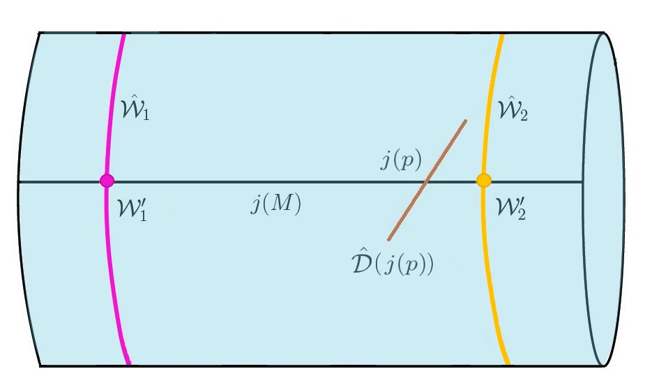
Figure 2: The decomposition of $M$ induced by $\hat{\mathcal{D}}$. The figure shows the particular case when each of the loci $\hat{\mathcal{W}}_{1}$ and $\hat{\mathcal{W}}_{2}$ (depicted in magenta and yellow respectively) is connected. The open stratum $\hat{\mathcal{U}}$ (depicted in cyan) defined by $\hat{\mathcal{D}}$ is the complement of $\hat{\mathcal{W}}=\hat{\mathcal{W}}_{1}\sqcup\hat{\mathcal{W}}_{2}$ inside ${\hat{M}}$. The intersection of $\hat{\mathcal{W}}_{k}$ with $j(M)$ determines loci $\mathcal{W}^{\prime}_{k}\subset M$, which in this low-dimensional rendering are depicted as dots. The intersection of $\hat{\mathcal{U}}$ with $j(M)$ determines the locus $\mathcal{U}^{\prime}\subset M$, which is the complement of the union $\mathcal{W}^{\prime}=\mathcal{W}^{\prime}_{1}\sqcup\mathcal{W}^{\prime}_{2}$ in $M$. In brown, we depicted the space $\hat{\mathcal{D}}(j(p))\subset T_{j(p)}{\hat{M}}$ for a point $p\in M$.

Using (16), the Gram determinant formula gives:

$$||{\hat{V}}_{1}\wedge{\hat{V}}_{2}\wedge{\hat{V}}_{3}||^{2}=\det\left[\begin{array}[]{ccc}1{}&~{}\hat{\alpha}&0\\ \hat{\alpha}{}&~{}1&0\\ 0&0&\frac{1-\hat{\alpha}}{2}\end{array}\right]=\frac{1}{2}(1+{\hat{\alpha}})(1-{\hat{\alpha}})^{2}~{}~{},$$ (31)

where we introduced the function (this is denoted by $\alpha$ in Palti ):

$${\hat{\alpha}}\stackrel{{\scriptstyle{\rm def.}}}{{=}}\langle{\hat{V}}_{1},{\hat{V}}_{2}\rangle\in\mathcal{C}^{\infty}({\hat{M}},[-1,1])~{}~{}.$$ (32)

Notice that $\hat{\alpha}$ is invariant under rotations of the circle and hence:

$${\hat{\alpha}}=\alpha\circ\pi_{1}~{}~{}\mathrm{for~{}some~{}function}~{}~{}\alpha\in\mathcal{C}^{\infty}(M,\mathbb{R})~{}~{}.$$

Relation (31) implies that the decomposition (26) of ${\hat{M}}$ coincides with the $\hat{\alpha}$-preimage of the canonical Whitney stratification of the closed interval $[-1,1]$:

$$\hat{\mathcal{U}}=\hat{\alpha}^{-1}((-1,1))=\{{\hat{p}}\in{\hat{M}}|~{}\hat{\alpha}({\hat{p}})\in(-1,1)\}~{}~{},~{}~{}\hat{\mathcal{W}}=\hat{\alpha}^{-1}(\{-1,1\})=\{{\hat{p}}\in{\hat{M}}|~{}|\hat{\alpha}({\hat{p}})|=1\}~{}~{},$$

while the first decomposition of $M$ given in (30) coincides with the $\alpha$-preimage of the same stratification:

$$\mathcal{U}^{\prime}=\alpha^{-1}((-1,1))=\{p\in M|~{}\alpha(p)\in(-1,1)\}~{}~{},~{}~{}\mathcal{W}^{\prime}=\alpha^{-1}(\{-1,1\})=\{p\in M|~{}|\alpha(p)|=1\}~{}~{}.$$

The following result (cf. Palti ) shows that the rank stratification of ${\hat{M}}$ induced by $\hat{\mathcal{D}}$ coincides with the $\hat{\alpha}$-preimage of the connected refinement of the Whitney stratification of the interval, while the stratification of $M$ given by the second decomposition in (30) coincides with the $\alpha$-preimage of the same.

Proposition.

Let ${\hat{p}}\in\hat{\mathcal{W}}$.

• For $\hat{\alpha}({\hat{p}})=+1$, we have ${\hat{V}}_{3}({\hat{p}})=0$ and ${\hat{V}}_{1}({\hat{p}})={\hat{V}}_{2}({\hat{p}})$ with $||{\hat{V}}_{1}({\hat{p}})||=1$. Thus ${\rm rk}\hat{\mathcal{D}}({\hat{p}})=8$.

• For $\hat{\alpha}({\hat{p}})=-1$, we have ${\hat{V}}_{2}({\hat{p}})=-{\hat{V}}_{1}({\hat{p}})$ with $||{\hat{V}}_{1}({\hat{p}})||=||{\hat{V}}_{3}({\hat{p}})||=1$ and ${\hat{V}}_{3}({\hat{p}})\perp{\hat{V}}_{1}({\hat{p}})$. Thus ${\rm rk}\hat{\mathcal{D}}({\hat{p}})=7$.

In particular, we have:

$$\hat{\mathcal{W}}_{1}=\hat{\alpha}^{-1}(\{+1\})=\{{\hat{p}}\in{\hat{M}}|\hat{\alpha}({\hat{p}})=+1\}~{},~{}\hat{\mathcal{W}}_{2}=\hat{\alpha}^{-1}(\{-1\})=\{{\hat{p}}\in{\hat{M}}|\hat{\alpha}({\hat{p}})=-1\}~{}~{}$$

$$\mathcal{W}^{\prime}_{1}=\alpha^{-1}(\{+1\})=\{p\in M|\alpha(p)=+1\}~{},~{}\mathcal{W}^{\prime}_{2}=\alpha^{-1}(\{-1\})=\{p\in M|\alpha(p)=-1\}~{}.~{}~{}~{}~{}~{}$$ (33)

Proof. Follows immediately from (16).$\blacksquare$

The following statement given in Palti follows from known facts about stabilizers of actions of Lie groups on spheres:

Proposition.

The isomorphism type of ${\hat{H}}_{\hat{p}}$ is given by (see Table 1):

• ${\hat{H}}_{\hat{p}}\simeq\mathrm{SU}(4)$ for ${\hat{p}}\in\hat{\mathcal{W}}_{1}=\hat{\alpha}^{-1}(\{+1\})$

• ${\hat{H}}_{\hat{p}}\simeq\mathrm{G_{2}}$ for ${\hat{p}}\in\hat{\mathcal{W}}_{2}=\hat{\alpha}^{-1}(\{-1\})$

• ${\hat{H}}_{\hat{p}}\simeq\mathrm{SU}(3)$ for ${\hat{p}}\in\hat{\mathcal{U}}=\hat{\alpha}^{-1}((-1,1))$  .

$\hat{\alpha}({\hat{p}})$	$\beta(\pi_{1}({\hat{p}}))$	$B^{-1}$-stratum	$\pi_{1}$-projection	${\rm rk}\hat{\mathcal{D}}({\hat{p}})$	${\hat{H}}_{\hat{p}}$
$+1$	$0$	$\hat{\mathcal{W}}_{1}$	$\mathcal{W}^{\prime}_{1}$	$8$	$\mathrm{SU}(4)$
$-1$	$1$	$\hat{\mathcal{W}}_{2}$	$\mathcal{W}^{\prime}_{2}$	$7$	$\mathrm{G_{2}}$
$\in(-1,1)$	$\in(0,1)$	$\hat{\mathcal{U}}$	$\mathcal{U}^{\prime}$	$6$	$\mathrm{SU}(3)$

Table 1: The stabilizer stratification of ${\hat{M}}$. The second column of the table uses relation (34).

In particular, the stabilizer stratification of ${\hat{M}}$ coincides with the rank stratification of $\hat{\mathcal{D}}$ and hence with the $\hat{\alpha}$-preimage of the canonical Whitney stratification of the interval $[-1,1]$ (see Figure 3).

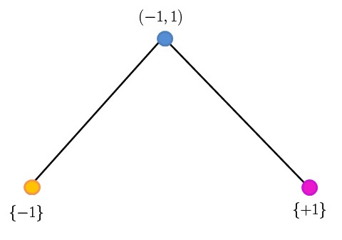
Figure 3: Hasse diagram of the incidence poset (see (msing, , Appendix C)) of the connected refinement of the Whitney stratification of the interval $[-1,1]$. The $\hat{\alpha}$-preimages of the strata depicted in magenta, yellow and cyan correspond to the $\mathrm{SU}(4)$, $\mathrm{G_{2}}$ and $\mathrm{SU}(3)$ loci of ${\hat{M}}$ respectively.

2.6 Comparison with the stratification of $M$ induced by the connected refinement of the Whitney stratification of $\mathfrak{P}$

Let $\beta:M\rightarrow\mathbb{R}$ be the function defined in (4).

Proposition.

We have:

$$\alpha=\langle V_{1},V_{2}\rangle+b_{1}b_{2}=1-2\beta^{2}\in\mathcal{C}^{\infty}(M,[-1,1])~{}~{}$$ (34)

and hence $\beta(M)\subset[0,1]$ and:

$$\begin{split}&\mathcal{U}^{\prime}=\beta^{-1}((0,1))~{}~{},~{}~{}\mathcal{W}^{\prime}_{1}=\beta^{-1}(\{0\})~{}~{},~{}~{}\mathcal{W}^{\prime}_{2}=\beta^{-1}(\{+1\})~{}~{}.\end{split}$$ (35)

Moreover, the following relations express $\mathcal{W}^{\prime}_{1},\mathcal{W}^{\prime}_{2},\mathcal{W}^{\prime}$ and $\mathcal{U}^{\prime}$ in terms of the strata introduced in (msing, , Subsection 5.3):

$$\begin{split}&\mathcal{W}^{\prime}_{1}=B^{-1}(\mathfrak{I})=\mathcal{W}_{0}\sqcup\mathcal{W}_{1}^{0}~{},~{}~{}\mathcal{W}^{\prime}_{2}=B^{-1}(\mathfrak{D})=\mathcal{W}_{1}^{1}\sqcup\mathcal{W}_{2}^{2+}~{}\\ &\mathcal{W}^{\prime}=\mathcal{W}_{0}\sqcup\mathcal{W}_{1}\sqcup\mathcal{W}_{2}^{2+}~{}~{},~{}~{}\mathcal{U}^{\prime}=B^{-1}(\mathrm{Int}\mathfrak{P})\sqcup B^{-1}(\mathfrak{A})\sqcup B^{-1}(\partial_{3}\mathfrak{P})=\mathcal{U}\sqcup\mathcal{W}_{2}^{2-}\sqcup\mathcal{W}_{2}^{3}\end{split}~{}~{}.$$ (36)

Proof. Relation (34) follows from (32) and (14), where the last equality in (34) follows by subtracting the second equation of (3) from the first and using (4) and (2). Relations (35) follow immediately from (2.5) upon using (34). The equalities in (36) follow immediately from the last two equations in (35) upon using the last Proposition in (msing, , Subsection 4.2) and the results of (msing, , Subsection 5.3). $\blacksquare$

3 Transversality

3.1 Recovering $\mathcal{D}$ from $\hat{\mathcal{D}}$

To understand the relation between the rank stratifications of $\mathcal{D}$ and $\hat{\mathcal{D}}$, notice that (12), together with the obvious equality $j_{\ast}(TM)=\ker\theta|_{j(M)}$, imply that $\mathcal{D}$ can be recovered from $\hat{\mathcal{D}}$ through the relation $j_{\ast}(\mathcal{D})=\left(\hat{\mathcal{D}}|_{j(M)}\right)\cap j_{\ast}(TM)$. Identifying $M$ with $j(M)$ (and hence $TM$ with $j_{\ast}(TM)$), we can write this relation as (see Figure 2):

$$\mathcal{D}=\hat{\mathcal{D}}|_{M}\cap TM~{}~{}.$$ (37)

Also notice that $\mathcal{U}^{\prime}$ and $\mathcal{W}^{\prime}$ coincide with the generic and degeneration loci of the restricted distribution $\hat{\mathcal{D}}|_{M}$:

$$\mathcal{U}^{\prime}=\{p\in M|{\rm rk}\hat{\mathcal{D}}(p)=6\}~{}~{},~{}~{}\mathcal{W}^{\prime}=\{p\in M|{\rm rk}\hat{\mathcal{D}}(p)>6\}~{}~{}.$$

3.2 The transverse and non-transverse loci of $M$

Recall that two subspaces $K_{1}$ and $K_{2}$ of a vector space $K$ satisfy $\dim(K_{1}+K_{2})=\dim K_{1}+\dim K_{2}-\dim(K_{1}\cap K_{2})$ i.e. $\mathrm{codim}(K_{1}+K_{2})=\mathrm{codim}K_{1}+\mathrm{codim}K_{2}-\mathrm{codim}(K_{1}\cap K_{2})$, where $\mathrm{codim}$ denotes the codimension relative to $K$. Since $\dim(K_{1}\cap K_{2})\leq\min(\dim K_{1},\dim K_{2})$, we have $\max(\mathrm{codim}K_{1},\mathrm{codim}K_{2})\leq\mathrm{codim}(K_{1}\cap K_{2})\leq\mathrm{codim}K_{1}+\mathrm{codim}K_{2}$. The subspaces are called transverse when $\mathrm{codim}(K_{1}\cap K_{2})=\mathrm{codim}K_{1}+\mathrm{codim}K_{2}$, which is equivalent with $\mathrm{codim}(K_{1}+K_{2})=0$ i.e. with $K_{1}+K_{2}=K$. This condition defines a symmetric binary relation (the transversality relation) on the set of all subspaces of $K$. For $p\in M$, let $\pitchfork_{p}$ denote the transversality relation between subspaces of $T_{j(p)}{\hat{M}}$, and $\not\pitchfork_{p}$ denote its negation (the non-transversality relation).

Definition.

The transverse locus is the following subset of $M$:

$$\mathcal{T}\stackrel{{\scriptstyle{\rm def.}}}{{=}}\{p\in M|\hat{\mathcal{D}}(p)\pitchfork_{p}T_{p}M\}~{}~{},$$ (38)

while its complement in $M$ is called the non-transverse locus:

$$\mathcal{N}\stackrel{{\scriptstyle{\rm def.}}}{{=}}\{p\in M|\hat{\mathcal{D}}(p)\not\pitchfork_{p}T_{p}M\}~{}~{},$$ (39)

where we identify $p\in M$ with $j(p)\in{\hat{M}}$ and $T_{p}M$ with the subspace $j_{\ast,p}(T_{p}M)$ of $T_{j(p)}{\hat{M}}$.

3.3 Characterizing the transverse and non-transverse loci

Proposition.

Let $p\in M\equiv j(M)$. Then:

$$\dim\mathcal{D}(p)\in\{\dim\hat{\mathcal{D}}(p),\dim\hat{\mathcal{D}}(p)-1\}~{}~{}.$$ (40)

Moreover, the following statements are equivalent:

1. $p\in\mathcal{N}$

2. $\dim\mathcal{D}(p)=\dim\hat{\mathcal{D}}(p)$

3. $\mathcal{D}(p)=\hat{\mathcal{D}}(p)$

4. $\hat{\mathcal{D}}(p)\subset T_{p}M$

5. $\theta(p)\in\langle{\hat{V}}_{1}(p),{\hat{V}}_{2}(p),{\hat{V}}_{3}(p)\rangle$ .

In particular, we have $\dim\mathcal{D}(p)=\dim\hat{\mathcal{D}}(p)-1$ iff $p\in\mathcal{T}$.

Proof. Since $T_{p}{\hat{M}}$ has dimension nine while $T_{p}M$ has dimension eight (thus $\mathrm{codim}T_{p}M=1$), relation (37) implies $\mathrm{codim}\mathcal{D}(p)\leq\mathrm{codim}\hat{\mathcal{D}}(p)+1$, i.e. $\dim\mathcal{D}(p)\geq\dim\hat{\mathcal{D}}(p)-1$, with equality iff $\hat{\mathcal{D}}(p)$ and $T_{p}M$ are transverse inside $T_{p}{\hat{M}}$. Since $\mathcal{D}(p)=\hat{\mathcal{D}}(p)\cap T_{p}M$, we have $\dim\mathcal{D}(p)\leq\dim\hat{\mathcal{D}}(p)$. This gives (40) and shows that:

$$\hat{\mathcal{D}}(p)\pitchfork T_{p}M~{}~{}\mathrm{iff}~{}~{}\dim\mathcal{D}(p)=\dim\hat{\mathcal{D}}(p)-1~{}~{}.$$

The non-transverse case corresponds to $\dim\mathcal{D}(p)=\dim\hat{\mathcal{D}}(p)$, which is equivalent with $\mathcal{D}(p)=\hat{\mathcal{D}}(p)$ since $\mathcal{D}(p)$ is a subspace of $\hat{\mathcal{D}}(p)$. Since $\mathcal{D}(p)=\hat{\mathcal{D}}(p)\cap T_{p}M\subset T_{p}M$, the equality $\mathcal{D}(p)=\hat{\mathcal{D}}(p)$ holds iff $\hat{\mathcal{D}}(p)\subset T_{p}M$. Since $T_{p}M=\ker\theta(p)$ and $\hat{\mathcal{D}}(p)=\cap_{i=1}^{3}\ker{\hat{V}}_{i}(p)$, this happens iff $\cap_{i=1}^{3}\ker{\hat{V}}_{i}(p)\subset\ker\theta(p)$, which by duality (taking polars) happens iff $\theta(p)\in\langle{\hat{V}}_{1}(p),{\hat{V}}_{2}(p),{\hat{V}}_{3}(p)\rangle$. $\blacksquare$

Corollary.

Let $p\in M\equiv j(M)$. Then the following statements are equivalent:

1. $p\in\mathcal{N}$.

2. There exist $\lambda_{1},\lambda_{2},\lambda_{3}\in\mathbb{R}$ such that:

   $$\lambda_{1}V_{1}(p)+\lambda_{2}V_{2}(p)+\lambda_{3}V_{3}(p)=0~{}~{}\mathrm{and}~{}~{}\lambda_{1}b_{1}(p)+\lambda_{2}b_{2}(p)+\lambda_{3}b_{3}(p)=1~{}~{}.$$

   In particular, the non-transverse locus is contained in the degeneration locus of $\mathcal{D}$ and hence the generic locus of $\mathcal{D}$ is contained in the transverse locus:

   $$\mathcal{N}\subset\mathcal{W}~{}~{},~{}~{}\mathcal{U}\subset\mathcal{T}~{}~{}.$$ (41)

Proof. Follows immediately from (12) and from the characterization of non-transversality given at point (e) of the previous proposition, using the fact that $\theta(p)$ is orthogonal to $V_{k}(p)$. $\blacksquare$

3.4 Expressing $\mathcal{T}$ and $\mathcal{N}$ through the preimage of the connected refinement of the Whitney stratification of $\mathfrak{P}$

Proposition.

The transverse and non-transverse loci are given by the following unions of the strata introduced in (msing, , Subsection 5.3):

$$\mathcal{T}=\mathcal{W}_{1}^{0}\sqcup\mathcal{W}_{2}^{2+}\sqcup\mathcal{U}~{}~{},~{}~{}\mathcal{N}=\mathcal{W}_{0}\sqcup\mathcal{W}_{1}^{1}\sqcup\mathcal{W}_{2}^{2-}\sqcup\mathcal{W}_{2}^{3}~{}~{}$$ (42)

and we have the relations:

$$\begin{split}&\mathcal{U}^{\prime}\cap\mathcal{T}=~{}~{}\mathcal{U}~{}~{}~{}~{},~{}~{}\mathcal{U}^{\prime}\cap\mathcal{N}=\mathcal{W}_{2}^{2-}\sqcup\mathcal{W}_{2}^{3}~{}~{}\\ &\mathcal{W}^{\prime}_{1}\cap\mathcal{T}=\mathcal{W}_{1}^{0}~{}~{},~{}~{}\mathcal{W}^{\prime}_{1}\cap\mathcal{N}=\mathcal{W}_{0}\\ &\mathcal{W}^{\prime}_{2}\cap\mathcal{T}=\mathcal{W}_{2}^{2+}~{},~{}\mathcal{W}^{\prime}_{2}\cap\mathcal{N}=\mathcal{W}_{1}^{1}~{}~{}.\end{split}$$ (43)

Proof. Follows immediately by comparing the ranks of $\hat{\mathcal{D}}|_{M}$ and $\mathcal{D}$ on various loci and using relations (36), the characterization of non-transversality given in the previous subsection and the results summarized in Tables 5 and 6 of msing . $\blacksquare$

The situation is summarized in Table 2.

$\mathfrak{P}$-locus	$\hat{\mathcal{D}}$-stratum	$B^{-1}$-stratum	$\mathcal{D}_{0}$-stratum	${\rm rk}\hat{\mathcal{D}}$	${\rm rk}\mathcal{D}$	${\rm rk}\mathcal{D}_{0}$	transversality	${\hat{H}}_{p}$	$H_{p}$
$\partial_{0}\mathfrak{P}=\partial\mathfrak{I}$	$\mathcal{W}^{\prime}_{1}$	$\mathcal{W}_{0}$	$\mathcal{Z}_{0}$	$8$	$8$	$8$	$\mathcal{N}$	$\mathrm{SU}(4)$	$\mathrm{SU}(4)$
$\partial_{1}^{0}\mathfrak{P}=\mathrm{Int}\mathfrak{I}$	$\mathcal{W}^{\prime}_{1}$	$\mathcal{W}_{1}^{0}$	$\mathcal{Z}_{2}$	$8$	$7$	$6$	$\mathcal{T}$	$\mathrm{SU}(4)$	$\mathrm{SU}(3)$
$\partial_{1}^{1}\mathfrak{P}=\partial\mathfrak{D}$	$\mathcal{W}^{\prime}_{2}$	$\mathcal{W}_{1}^{1}$	$\mathcal{Z}_{1}$	$7$	$7$	$7$	$\mathcal{N}$	$\mathrm{G_{2}}$	$\mathrm{G_{2}}$
$\mathrm{Int}\mathfrak{D}\subset\partial_{2}\mathfrak{P}$	$\mathcal{W}^{\prime}_{2}$	$\mathcal{W}_{2}^{2+}$	$\mathcal{Z}_{2}$	$7$	$6$	$6$	$\mathcal{T}$	$\mathrm{G_{2}}$	$\mathrm{SU}(3)$
$\mathfrak{A}\sqcup\partial_{3}\mathfrak{P}$	$\mathcal{U}^{\prime}$	$\mathcal{W}_{2}^{2-}\sqcup\mathcal{W}_{2}^{3}$	$\mathcal{Z}_{2}$	$6$	$6$	$6$	$\mathcal{N}$	$\mathrm{SU}(3)$	$\mathrm{SU}(3)$
$\mathrm{Int}\mathfrak{P}$	$\mathcal{U}^{\prime}$	$\mathcal{U}$	$\mathcal{U}$	$6$	$5$	$4$	$\mathcal{T}$	$\mathrm{SU}(3)$	$\mathrm{SU}(2)$

Table 2: The ranks of $\hat{\mathcal{D}}|_{M},\mathcal{D}$ and $\mathcal{D}_{0}$ on various loci of $M$ and the character of the intersection $\hat{\mathcal{D}}|_{M}\cap TM$. The stabilizer groups on ${\hat{M}}$ and $M$ are shown in the last two columns.

Remark.

The proposition implies:

$$\begin{split}&\mathcal{U}=\{p\in M|{\rm rk}\hat{\mathcal{D}}(p)=6~{}and~{}\hat{\mathcal{D}}(p)~{}\mathrm{intersects}~{}T_{p}M~{}\mathrm{transversely}\}=\mathcal{U}^{\prime}\cap\mathcal{T}\\ &\mathcal{W}=\{p\in M|{\rm rk}\hat{\mathcal{D}}(p)>6~{}~{}or~{}~{}\hat{\mathcal{D}}(p)~{}\mathrm{intersects}~{}T_{p}M~{}\mathrm{non-transversely}\}=\mathcal{W}^{\prime}\cup\mathcal{N}~{}~{}.\end{split}$$

In particular, the $\mathrm{SU}(2)$ stratum $\mathcal{U}$ of $M$ is the intersection of the $\mathrm{SU}(3)$ stratum $\hat{\mathcal{U}}$ of ${\hat{M}}$ with the locus $j(\mathcal{T})\subset j(M)$, while the degeneration points of $\mathcal{D}$ (the points of the locus $\mathcal{W}\subset M$) are of three kinds:

• The points $p\in\mathcal{W}^{\prime}_{1}=\mathcal{W}_{0}\sqcup\mathcal{W}_{1}^{0}$ (where $\beta=0$ i.e. $\alpha=+1$), which form the intersection of the $\mathrm{SU}(4)$ stratum $\hat{\mathcal{W}}_{1}$ of ${\hat{M}}$ with $j(M)$. At such points, we have $H_{p}\simeq\mathrm{SU}(4)$ or $\mathrm{SU}(3)$ according to whether $p\in\mathcal{N}$ or $p\in\mathcal{T}$.

• The points of $\mathcal{W}^{\prime}_{2}=\mathcal{W}_{1}^{1}\sqcup\mathcal{W}_{2}^{2+}$ (where $\beta=1$ i.e. $\alpha=-1$), which form the intersection of the $\mathrm{G_{2}}$ stratum $\hat{\mathcal{W}}_{2}$ of ${\hat{M}}$ with $j(M)$. At such points, we have $H_{p}\simeq\mathrm{G_{2}}$ or $\mathrm{SU}(3)$ according to whether $p\in\mathcal{N}$ or $p\in\mathcal{T}$.

• The points of $\mathcal{W}\setminus\mathcal{W}^{\prime}=\mathcal{W}_{2}^{2-}\sqcup\mathcal{W}_{2}^{3}$, which form the intersection of the $\mathrm{SU}(3)$ stratum $\hat{\mathcal{U}}$ of ${\hat{M}}$ with the locus $j(\mathcal{N})\subset j(M)$. At such points, we have $H_{p}\simeq\mathrm{SU}(3)$.

3.5 The case $\mathcal{T}=\emptyset$

The previous proposition immediately implies the following:

Corollary.

The condition $\mathcal{T}=\emptyset$ is equivalent with the conditions $\mathcal{W}_{1}^{0}=\mathcal{W}_{2}^{2+}=\mathcal{U}=\emptyset$. When this condition is satisfied, we have $\mathcal{W}^{\prime}_{1}=\mathcal{Z}_{0}=\mathcal{W}_{0}$, $\mathcal{W}^{\prime}_{2}=\mathcal{Z}_{1}=\mathcal{W}_{1}^{1}$ and $\mathcal{U}^{\prime}=\mathcal{Z}_{2}=\mathcal{W}_{2}^{2-}\sqcup\mathcal{W}_{2}^{3}$. In this case, we have $M=\mathcal{N}=\mathcal{W}_{0}\sqcup\mathcal{W}_{1}^{1}\sqcup\mathcal{W}_{2}^{2-}\sqcup\mathcal{W}_{2}^{3}$ and ${\hat{H}}_{p}\simeq H_{p}$ for any $p\in M$, both groups being isomorphic with $\mathrm{SU}(4)$, $\mathrm{G_{2}}$ or $\mathrm{SU}(3)$ according to whether $p\in\mathcal{W}_{0}$, $p\in\mathcal{W}_{1}^{1}$ or $p\in\mathcal{W}_{2}^{2-}\sqcup\mathcal{W}_{2}^{3}$.

Notice that $\mathcal{T}=\emptyset$ implies $B^{-1}(\mathrm{Int}\mathfrak{P})=\mathcal{U}=\emptyset$ and hence requires that the image of $B$ be contained in the frontier $\partial\mathfrak{P}$ of $\mathfrak{P}$. More precisely, we have:

$$\mathcal{T}=\emptyset~{}~{}\mathrm{iff}~{}~{}B(M)\subset\partial\mathfrak{I}\sqcup\partial\mathfrak{D}\sqcup\mathfrak{A}\sqcup\partial_{3}\mathfrak{P}~{}~{}.$$

Remark.

Reference Palti uses the assumption (see equation (3.9) of loc. cit.) that $\theta(p)$ is a linear combination of ${\hat{V}}_{1}(p),{\hat{V}}_{2}(p)$ and ${\hat{V}}_{3}(p)$ for every point $p\in M$. By the characterization given at point (e) of the Proposition of Subsection 3.3, this assumption is equivalent with the requirement that the transverse locus $\mathcal{T}$ be empty and hence that we are in the setting of the Corollary above. By the Corollary of Subsection 3.3, the condition $\mathcal{T}=\emptyset$ requires, in particular, that the 1-forms $V_{1}(p),V_{2}(p)$ and $V_{3}(p)$ be linearly dependent at every point $p\in M$ (cf. (msing, , Appendix G)). In was shown in msing that, generically, we have $\mathcal{U}\neq\emptyset$ and hence the transverse locus is not empty in the generic case.

3.6 Relation between the stabilizer stratifications of $M$ and ${\hat{M}}$

It is known that an orientable hypersurface in an 8-manifold with $\mathrm{SU}(4)$ structure carries a naturally induced $\mathrm{SU}(3)$ structure (see, for example, (FinoTomassini, , Section 4)). An orientable hypersurface in a 7-manifold with $\mathrm{G_{2}}$ structure carries a naturally induced $\mathrm{SU}(3)$ structure (see, for example, CabreraSU3 ; ChiossiSalamon ; Knotes ). Finally, an orientable hypersurface of a manifold with $\mathrm{SU}(3)$ structure carries a naturally induced $\mathrm{SU}(2)$ structure ContiSalamon . Since these statements are purely algebraic, they extend immediately to the case of Frobenius distributions. Using these facts and the results above, we can understand how the stratified G-structure of ${\hat{M}}$ induces the stratified G-structure of $M$. Namely, we have (see Table 2):

• The restriction $\mathcal{D}|_{\mathcal{N}}$ coincides with $\hat{\mathcal{D}}|_{\mathcal{N}}$ and hence $\mathcal{D}|_{\mathcal{N}}$ carries the same structure group (namely $\mathrm{SU}(4)$, $\mathrm{G_{2}}$ or $\mathrm{SU}(3)$) as $\hat{\mathcal{D}}|_{\mathcal{N}}$ on the components $\mathcal{W}_{0}$, $\mathcal{W}_{1}^{1}$ and $\mathcal{W}_{2}^{2-}\sqcup\mathcal{W}_{2}^{3}$ respectively of the non-transverse locus.

• The restriction $\mathcal{D}|_{\mathcal{T}}$ is an orientable and corank one generalized sub-distribution of $\hat{\mathcal{D}}|_{\mathcal{T}}$ and hence $\mathcal{D}|_{\mathcal{T}}$ carries the structure group $\mathrm{SU}(3)$, $\mathrm{SU}(3)$ and $\mathrm{SU}(2)$ on the components $\mathcal{W}_{1}^{0}$, $\mathcal{W}_{2}^{2+}$ and $\mathcal{U}$ respectively of the transverse locus $\mathcal{T}$ on which $\hat{\mathcal{D}}|_{\mathcal{T}}$ has the structure group $\mathrm{SU}(4)$, $\mathrm{G_{2}}$ and $\mathrm{SU}(3)$ respectively.

These observations give a different way to understand the results of msing , provided that one knows the codimension of $\mathcal{D}(p)$ inside $\hat{\mathcal{D}}(p)$ on the various strata (which follows from loc. cit.).

4 Explicit relation between the $\mathrm{SU}(3)$ structure on $\hat{\mathcal{U}}$ and the $\mathrm{SU}(2)$ structure on $\mathcal{U}$

Since $j$ identifies $\mathcal{U}=\mathcal{U}^{\prime}\cap\mathcal{T}$ with $\hat{\mathcal{U}}\cap j(\mathcal{T})$, the restriction of $\hat{\mathcal{D}}$ to the locus $\mathcal{U}\equiv j(\mathcal{U})\subset\hat{\mathcal{U}}$ is a regular Frobenius distribution of rank six. Since ${\hat{M}}$ is oriented with volume form (9), we can orient $\hat{\mathcal{D}}|_{\mathcal{U}}$ using the volume form:

$${\hat{\nu}}_{\perp}\stackrel{{\scriptstyle{\rm def.}}}{{=}}\frac{1}{||{\hat{V}}_{+}\wedge{\hat{V}}_{-}\wedge{\hat{V}}_{3}||}\iota_{{\hat{V}}_{+}\wedge{\hat{V}}_{-}\wedge{\hat{V}}_{3}}{\hat{\nu}}|_{\mathcal{U}}~{}~{}.$$ (44)

4.1 The projection of $\theta$ along $\hat{\mathcal{D}}$ on the generic locus

The one-form $\theta|_{\mathcal{U}}$ decomposes uniquely as:

$$\theta|_{\mathcal{U}}=\theta_{\perp}+\theta_{\parallel}~{}~{},$$ (45)

where $\theta_{\perp}\in\Omega^{1}_{\mathcal{U}}(\hat{\mathcal{D}})=\langle{\hat{V}}_{+}|_{\mathcal{U}},{\hat{V}}_{-}|_{\mathcal{U}},{\hat{V}}_{3}|_{\mathcal{U}}\rangle^{\perp}$ and $\theta_{\parallel}\in\Omega^{1}_{\mathcal{U}}(\hat{\mathcal{D}}^{\perp})=\langle{\hat{V}}_{+}|_{\mathcal{U}},{\hat{V}}_{-}|_{\mathcal{U}},{\hat{V}}_{3}|_{\mathcal{U}}\rangle$ (see Figure 4). Since $\mathcal{U}$ is a subset of $\mathcal{T}$, the characterization at point (e) of the Proposition of Subsection 3.3 gives $\theta|_{\mathcal{U}}\not\in\langle{\hat{V}}_{+}|_{\mathcal{U}},{\hat{V}}_{-}|_{\mathcal{U}},{\hat{V}}_{3}|_{\mathcal{U}}\rangle$ and hence $\theta_{\perp}\neq 0$ and we can define the unit norm one-form:

$${\mathbf{n}}\stackrel{{\scriptstyle{\rm def.}}}{{=}}\frac{\theta_{\perp}}{||\theta_{\perp}||}\in\Omega^{1}_{\mathcal{U}}(\hat{\mathcal{D}})~{}~{}.$$ (46)

We orient the rank five Frobenius distribution $\mathcal{D}|_{\mathcal{U}}$ such that its volume form is given by:

$$\nu_{\perp}=-\frac{1}{||V_{+}\wedge V_{-}\wedge V_{3}||}\iota_{V_{+}\wedge V_{-}\wedge V_{3}}\nu~{}~{}.$$ (47)

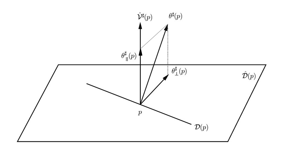
Figure 4: Construction of $\theta_{\perp}(p)$ for $p\in\mathcal{U}\equiv j(\mathcal{U})\subset j(M)\subset{\hat{M}}$. The vectors $\theta^{\sharp}(p)\in T_{p}{\hat{M}}$ and $\theta_{\perp}^{\sharp}(p)\in T_{p}{\hat{M}}$ shown in the figure are obtained by applying the musical isomorphism of $({\hat{M}},{\hat{g}})$ to the 1-forms $\theta(p)$ and $\theta_{\perp}(p)$. The vertical arrow represents the space ${\hat{\mathcal{V}}}^{\sharp}(p)$ spanned by the vectors ${\hat{V}}_{1}^{\sharp}(p),{\hat{V}}_{2}^{\sharp}(p)$ and ${\hat{V}}_{3}^{\sharp}(p)$ inside $T_{p}{\hat{M}}$. The vectors $\theta_{\perp}^{\sharp}(p)$ and $\theta_{\parallel}^{\sharp}(p)$ are the orthogonal projections of $\theta^{\sharp}(p)$ onto $\hat{\mathcal{D}}(p)$ and ${\hat{\mathcal{V}}}^{\sharp}(p)$ respectively. The subspace $\mathcal{D}(p)$ of $T_{p}{\hat{M}}$ coincides with the intersection of $\hat{\mathcal{D}}(p)$ with $T_{p}M=\ker\theta(p)\subset T_{p}{\hat{M}}$ and hence it is orthogonal to the vector $\theta^{\sharp}(p)\in T_{p}{\hat{M}}$. It is also orthogonal to the subspace ${\hat{\mathcal{V}}}^{\sharp}(p)\subset T_{p}{\hat{M}}$.

Proposition.

We have $\mathcal{D}|_{\mathcal{U}}=(\ker\theta_{\perp})\cap\hat{\mathcal{D}}|_{\mathcal{U}}$, i.e. the normalized vector field ${\mathbf{n}}^{\sharp}\in\Gamma(\mathcal{U},\hat{\mathcal{D}})$ is everywhere orthogonal to $\mathcal{D}|_{\mathcal{U}}$ inside $\hat{\mathcal{D}}|_{\mathcal{U}}$, where $~{}^{\sharp}$ denotes the musical isomorphism of $({\hat{M}},{\hat{g}})$. Moreover, we have:

$$||\theta_{\perp}||=\frac{||V_{+}\wedge V_{-}\wedge V_{3}||}{||{\hat{V}}_{+}\wedge{\hat{V}}_{-}\wedge{\hat{V}}_{3}||}$$ (48)

and:

$$\nu_{\perp}=-\iota_{\mathbf{n}}{\hat{\nu}}_{\perp}~{}~{}.$$ (49)

Furthermore, we have:

$$\theta_{\parallel}=\frac{b_{+}}{1-\beta^{2}}{\hat{V}}_{+}+\frac{b_{-}}{\beta^{2}}{\hat{V}}_{-}+\frac{b_{3}}{\beta^{2}}{\hat{V}}_{3}~{}~{}(\mathrm{on}~{}\mathcal{U})$$ (50)

and:

$$||\theta_{\perp}||^{2}=1-\frac{b_{+}^{2}}{1-\beta^{2}}-\frac{\rho^{2}}{\beta^{2}}~{}~{}(\mathrm{on}~{}\mathcal{U})~{}~{},$$ (51)

where $\rho$ was defined in (21).

Proof. Since $\mathcal{D}\subset TM$, we have $\mathcal{D}|_{\mathcal{U}}\subset\ker\theta|_{\mathcal{U}}$ and hence $\theta$ vanishes on $\mathcal{D}|_{\mathcal{U}}$. Since $\theta_{\parallel}$ is a linear combination of ${\hat{V}}_{1}|_{\mathcal{U}},{\hat{V}}_{2}|_{\mathcal{U}}$ and ${\hat{V}}_{3}|_{\mathcal{U}}$ and since $\hat{\mathcal{D}}=\cap_{i=1}^{3}\ker{\hat{V}}_{i}$, we have $\hat{\mathcal{D}}|_{\mathcal{U}}\subset\ker\theta_{\parallel}$ and hence $\theta_{\parallel}$ vanishes on $\hat{\mathcal{D}}|_{\mathcal{U}}$ and thus also on $\mathcal{D}|_{\mathcal{U}}\subset\hat{\mathcal{D}}|_{\mathcal{U}}$. Using relation (45), the fact that $\theta|_{\mathcal{U}}$ and $\theta_{\parallel}$ vanish on $\mathcal{D}|_{\mathcal{U}}$ implies that $\theta_{\perp}$ vanishes on $\mathcal{D}|_{\mathcal{U}}$ and hence that $\theta_{\perp}^{\sharp}$ and ${\mathbf{n}}^{\sharp}$ are orthogonal to $\mathcal{D}|_{\mathcal{U}}$. Relations (47) and (9) give:

$$\nu_{\perp}=-\frac{1}{||V_{+}\wedge V_{-}\wedge V_{3}||}\iota_{V_{+}\wedge V_{-}\wedge V_{3}\wedge\theta}{\hat{\nu}}|_{\mathcal{U}}=\frac{||{\hat{V}}_{+}\wedge{\hat{V}}_{-}\wedge{\hat{V}}_{3}||}{||V_{+}\wedge V_{-}\wedge V_{3}||}\iota_{\theta_{\perp}}{\hat{\nu}}_{\perp}~{}~{},$$ (52)

where in the second equality we used the relation (44) and the equality:

$$V_{+}\wedge V_{-}\wedge V_{3}\wedge\theta={\hat{V}}_{+}\wedge{\hat{V}}_{-}\wedge{\hat{V}}_{3}\wedge\theta=-\theta_{\perp}\wedge{\hat{V}}_{+}\wedge{\hat{V}}_{-}\wedge{\hat{V}}_{3}~{}~{},$$

which follows from the decompositions (12) and (45) upon noticing that ${\hat{V}}_{+}\wedge{\hat{V}}_{-}\wedge{\hat{V}}_{3}\wedge\theta_{\parallel}=0$. Relations (48) and (49) now follow from (52) upon noticing that $||\nu_{\perp}||=||{\hat{\nu}}_{\perp}||=1$ and $||\iota_{\theta_{\perp}}{\hat{\nu}}_{\perp}||=||\theta_{\perp}||||{\hat{\nu}}_{\perp}||=||\theta_{\perp}||$. The decomposition (45) means that $\theta_{\parallel}$ is the projection of $\theta$ onto $\langle{\hat{V}}_{+}|_{\mathcal{U}},{\hat{V}}_{-}|_{\mathcal{U}},{\hat{V}}_{3}|_{\mathcal{U}}\rangle$. Writing $\theta_{\parallel}=a_{+}{\hat{V}}_{+}|_{\mathcal{U}}+a_{-}{\hat{V}}_{-}|_{\mathcal{U}}+a_{3}{\hat{V}}_{3}|_{\mathcal{U}}$ with $a_{r}\in\mathcal{C}^{\infty}(\mathcal{U},\mathbb{R})$, we have $\langle\theta,{\hat{V}}_{r}\rangle|_{\mathcal{U}}=\langle\theta_{\parallel},{\hat{V}}_{r}\rangle|_{\mathcal{U}}=a_{r}||{\hat{V}}_{r}||^{2}|_{\mathcal{U}}$, where we used the fact that $\langle{\hat{V}}_{r},{\hat{V}}_{s}\rangle=||{\hat{V}}_{r}|||^{2}\delta_{rs}$ for all $r,s\in\{+,-,3\}$ (see (15)). On the other hand, relations (12) give $\langle\theta,{\hat{V}}_{r}\rangle|_{\mathcal{U}}=b_{r}$. Thus $a_{r}=\frac{b_{r}}{||{\hat{V}}_{r}||^{2}}$ on $\mathcal{U}$, i.e.:

$$a_{+}=\frac{b_{+}}{||{\hat{V}}_{+}||^{2}}=\frac{b_{+}}{1-\beta^{2}}~{}~{},~{}~{}a_{-}=\frac{b_{-}}{||{\hat{V}}_{-}||^{2}}=\frac{b_{-}}{\beta^{2}}~{}~{},~{}~{}a_{3}=\frac{b_{3}}{||{\hat{V}}_{3}||^{2}}=\frac{b_{3}}{\beta^{2}}~{}~{}(\mathrm{on}~{}\mathcal{U})~{}~{},$$

where we used (17). This immediately gives (50) and (51). Notice that relation (51) can also be derived from (48) by using the expression for the Gram determinant $||V_{+}\wedge V_{-}\wedge V_{3}||^{2}$ given in (msing, , Section 4.2) and the relation $||{\hat{V}}_{+}\wedge{\hat{V}}_{-}\wedge{\hat{V}}_{3}||^{2}=||{\hat{V}}_{+}||^{2}||{\hat{V}}_{-}||^{2}||{\hat{V}}_{3}||^{2}=\beta^{4}(1-\beta^{2})$ (which follows from (17)). Indeed, we have:

$$||\theta_{\perp}||^{2}=\frac{||V_{+}\wedge V_{-}\wedge V_{3}||^{2}}{||{\hat{V}}_{+}\wedge{\hat{V}}_{-}\wedge{\hat{V}}_{3}||^{2}}=-\frac{\beta^{2}(\beta^{4}-\beta^{2}(1-b_{+}^{2}+\rho^{2})+\rho^{2})}{\beta^{4}(1-\beta^{2})}=\frac{\beta^{2}(1-\beta^{2})-\beta^{2}b_{+}^{2}-\rho^{2}(1-\beta^{2})}{\beta^{2}(1-\beta^{2})}~{}~{},$$

which recovers (51). $\blacksquare$

Remark.

Relations (45), (46), (50) and (51) give:

$$\theta=_{\mathcal{U}}\frac{b_{+}}{1-\beta^{2}}{\hat{V}}_{+}+\frac{b_{-}}{\beta^{2}}{\hat{V}}_{-}+\frac{b_{3}}{\beta^{2}}{\hat{V}}_{3}+\sqrt{1-\frac{b_{+}^{2}}{1-\beta^{2}}-\frac{\rho^{2}}{\beta^{2}}}~{}{\mathbf{n}}~{}~{}.$$ (53)

Substituting (12) into this relation allows us to express $\theta|_{\mathcal{U}}$ in terms of $V_{+},V_{-},V_{3}$ and ${\mathbf{n}}$:

$$\theta=_{\mathcal{U}}\frac{\frac{b_{+}}{1-\beta^{2}}V_{+}-\frac{b_{-}}{\beta^{2}}V_{-}-\frac{b_{3}}{\beta^{2}}V_{3}}{1-\frac{b_{+}^{2}}{1-\beta^{2}}-\frac{\rho^{2}}{\beta^{2}}}+\frac{{\mathbf{n}}}{\sqrt{1-\frac{b_{+}^{2}}{1-\beta^{2}}-\frac{\rho^{2}}{\beta^{2}}}}~{}~{}.$$ (54)

Relation (53) should be compared with equation (3.9) of reference Palti , which holds only on the non-transverse locus $\mathcal{N}$ (and on its lift to ${\hat{M}}$). By contrast, equation (53) holds on the generic locus $\mathcal{U}$, which is contained in the transverse locus.

4.2 Relation between $\mathrm{SU}(2)$ and $\mathrm{SU}(3)$ structures

An $\mathrm{SU}(2)$ structure on the oriented rank five Frobenius distribution $\mathcal{D}|_{\mathcal{U}}$ which is compatible with the metric $g|_{\mathcal{D}}$ and with the orientation of $\mathcal{D}$ can be described by a normalized one-form ${\boldsymbol{\alpha}}\in\Omega^{1}_{\mathcal{U}}(\mathcal{D})$ and three mutually orthogonal 2-forms ${\boldsymbol{\omega}}_{1},{\boldsymbol{\omega}}_{2},{\boldsymbol{\omega}}_{3}\in\Omega^{2}_{\mathcal{U}}(\mathcal{D})$ satisfying the equations (see ContiSalamon ):

$$\begin{split}&~{}\iota_{\boldsymbol{\alpha}}{\boldsymbol{\omega}}_{k}=0\\ &\langle{\boldsymbol{\omega}}_{k},{\boldsymbol{\omega}}_{l}\rangle=2\delta_{kl}\\ &~{}{\boldsymbol{\omega}}_{k}\wedge{\boldsymbol{\omega}}_{l}=\delta_{kl}{\mathbf{v}}~{}~{},\end{split}~{}~{}$$ (55)

where $k,l=1,2,3$ and ${\mathbf{v}}$ is a non-vanishing four-form which satisfies:

$$\iota_{\boldsymbol{\alpha}}\nu_{\perp}=\frac{1}{2}{\mathbf{v}}~{}~{}\mathrm{i.e.}~{}~{}{\boldsymbol{\alpha}}\wedge{\mathbf{v}}=2\nu_{\perp}~{}~{}.$$

Namely, we have $\mathcal{D}_{0}|_{\mathcal{U}}=\ker{\boldsymbol{\alpha}}$ and $({\boldsymbol{\omega}}_{1},{\boldsymbol{\omega}}_{2},{\boldsymbol{\omega}}_{3})$ is an orthogonal basis of the free $\mathcal{C}^{\infty}(\mathcal{U},\mathbb{R})$-module $\Omega^{2+}_{\mathcal{U}}(\mathcal{D}_{0})$ of $\mathcal{D}_{0}|_{\mathcal{U}}$-longitudinal self-dual 2-forms. As explained in ContiSalamon , this basis can be chosen such that it forms a positively-oriented frame of the rank three bundle $\wedge^{2+}\mathcal{D}_{0}^{\ast}$, where the latter is endowed with the orientation naturally induced from that of $\mathcal{D}_{0}$ (which is given by the volume form $\frac{1}{2}{\mathbf{v}}$).

On the other hand, an $\mathrm{SU}(3)$ structure on the oriented rank six Frobenius distribution $\hat{\mathcal{D}}|_{\mathcal{U}}$ which is compatible with the metric ${\hat{g}}|_{\mathcal{D}}$ and with the orientation of $\hat{\mathcal{D}}$ is determined ChiossiSalamon by an almost complex structure $\mathbf{I}\in\Gamma(\mathcal{U},\mathrm{End}(\hat{\mathcal{D}}))$ which is compatible with the metric and orientation of $\hat{\mathcal{D}}$, together with a complex-valued three-form $\mathbf{\Omega}\in\Omega^{2}_{\mathcal{U}}(\hat{\mathcal{D}})\otimes\mathbb{C}$ which is of unit norm and has type $(3,0)$ with respect to $\mathbf{I}$. The almost complex structure defines a two-form $\mathbf{J}\in\Omega^{2}_{\mathcal{U}}(\hat{\mathcal{D}})$ through the relation:

$$\mathbf{J}(X,Y)\stackrel{{\scriptstyle{\rm def.}}}{{=}}{\hat{g}}(X,\mathbf{I}Y)~{}~{},~{}~{}\forall X,Y\in\Gamma(\mathcal{U},\hat{\mathcal{D}})~{}~{}$$ (56)

and this form satisfies:

$${\hat{\nu}}_{\perp}=_{\mathcal{U}}\frac{1}{6}\mathbf{J}\wedge\mathbf{J}\wedge\mathbf{J}~{}~{}.$$ (57)

The phase of the normalized (3,0)-form $\mathbf{\Omega}$ is fixed through the convention:

$$\mathbf{\Omega}\wedge\bar{\mathbf{\Omega}}=_{\mathcal{U}}-8\mathrm{i}{\hat{\nu}}_{\perp}~{}~{},$$ (58)

Decomposing $\mathbf{\Omega}$ into its real and imaginary parts:

$$\mathbf{\Omega}=\boldsymbol{\varphi}+i\boldsymbol{\rho}~{}~{}\mathrm{with}~{}~{}\boldsymbol{\varphi},\boldsymbol{\rho}\in\Omega^{3}_{\mathcal{U}}(\hat{\mathcal{D}})~{}~{},$$ (59)

relation (58) amounts to:

$$\boldsymbol{\varphi}\wedge\boldsymbol{\rho}=_{\mathcal{U}}4{\hat{\nu}}_{\perp}~{}~{}.$$ (60)

The following proposition gives the relation between $\mathrm{SU}(3)$ structures on the rank six Frobenius distribution $\hat{\mathcal{D}}|_{\mathcal{U}}\stackrel{{\scriptstyle{\rm def.}}}{{=}}j^{\ast}(\hat{\mathcal{D}})|_{\mathcal{U}}$ and $\mathrm{SU}(2)$ structures on its corank one sub-distribution $\mathcal{D}|_{\mathcal{U}}\subset\hat{\mathcal{D}}|_{\mathcal{U}}$.

Proposition.

There is a bijective correspondence between $\mathrm{SU}(3)$ structures on $\hat{\mathcal{D}}|_{\mathcal{U}}$ which are compatible with the metric and orientation of $\hat{\mathcal{D}}|_{\mathcal{U}}$ and $\mathrm{SU}(2)$ structures on $\mathcal{D}|_{\mathcal{U}}$ which are compatible with the metric and orientation of $\mathcal{D}|_{\mathcal{U}}$. This correspondence is given as follows, where ${\mathbf{n}}$ was defined in (46):

1. Given a metric- and orientation-compatible $\mathrm{SU}(3)$ structure on $\hat{\mathcal{D}}|_{\mathcal{U}}$ with 2-form $\mathbf{J}\in\Omega^{2}_{\mathcal{U}}(\hat{\mathcal{D}})$ and complex 3-form $\mathbf{\Omega}\in\Omega^{3}_{\mathcal{U}}(\hat{\mathcal{D}})\otimes\mathbb{C}$, the following formulas give the canonical forms defining the corresponding metric- and orientation-compatible $\mathrm{SU}(2)$ structure on $\mathcal{D}|_{\mathcal{U}}$, where $\mathrm{i}$ is the imaginary unit:

   $${\boldsymbol{\alpha}}=-\iota_{\mathbf{n}}\mathbf{J}|_{\mathcal{D}}\in\Omega^{1}_{\mathcal{U}}(\mathcal{D})~{}~{},~{}~{}{\boldsymbol{\omega}}_{1}=\mathbf{J}|_{\mathcal{D}}\in\Omega^{2}_{\mathcal{U}}(\mathcal{D})~{}~{},~{}~{}$$

   $${\boldsymbol{\omega}}_{2}+\mathrm{i}{\boldsymbol{\omega}}_{3}=-\mathrm{i}~{}\iota_{\mathbf{n}}\mathbf{\Omega}|_{\mathcal{D}}\in\Omega^{2}_{\mathcal{U}}(\mathcal{D})~{}~{}.$$

2. Given a metric- and orientation-compatible $\mathrm{SU}(2)$ structure on $\mathcal{D}|_{\mathcal{U}}$ which is defined by the canonical forms ${\boldsymbol{\alpha}}\in\Omega^{1}_{\mathcal{U}}(\mathcal{D})$ and ${\boldsymbol{\omega}}_{k}\in\Omega^{2}_{\mathcal{U}}(\mathcal{D})$ (where $k=1,2,3$), the following forms define the corresponding metric- and orientation-compatible $\mathrm{SU}(3)$ structure on $\hat{\mathcal{D}}|_{\mathcal{U}}$:

   $$\mathbf{J}={\boldsymbol{\omega}}_{1}+{\boldsymbol{\alpha}}\wedge{\mathbf{n}}\in\Omega^{2}_{\mathcal{U}}(\hat{\mathcal{D}})~{}~{},~{}~{}$$ (61)

   $$\mathbf{\Omega}=({\boldsymbol{\omega}}_{2}+\mathrm{i}{\boldsymbol{\omega}}_{3})\wedge({\boldsymbol{\alpha}}+\mathrm{i}{\mathbf{n}})\in\Omega^{3}_{\mathcal{U}}(\hat{\mathcal{D}})\otimes\mathbb{C}~{}~{}.$$ (62)

Proof. This is an obvious adaptation of (ContiSalamon, , Proposition 1.4) to the case of Frobenius distributions. Notice that the signs agree with our choices of orientation. Indeed, we have:

$${\boldsymbol{\alpha}}\wedge{\mathbf{v}}={\boldsymbol{\alpha}}\wedge{\boldsymbol{\omega}}_{1}\wedge{\boldsymbol{\omega}}_{1}=_{\mathcal{U}}-(\iota_{\mathbf{n}}\mathbf{J})\wedge\mathbf{J}\wedge\mathbf{J}|_{\mathcal{D}}=-\frac{1}{3}\iota_{\mathbf{n}}(\mathbf{J}\wedge\mathbf{J}\wedge\mathbf{J})|_{\mathcal{D}}=_{\mathcal{U}}-2\iota_{\mathbf{n}}{\hat{\nu}}_{\perp}=2\nu_{\perp}~{}~{}.$$

$\blacksquare$

4.3 Recovering the $\mathrm{SU}(2)$ structure on the generic locus of $M$

Reference Palti constructs an $\mathrm{SU}(3)$ structure on the rank six Frobenius distribution which is obtained by restricting $\hat{\mathcal{D}}$ to the open subset $\hat{\mathcal{U}}\subset{\hat{M}}$, a set which (by the results of Section 3) contains the $\pi_{1}^{-1}(\mathcal{U})$ of the generic locus. This $\mathrm{SU}(3)$ structure is described in loc. cit through certain differential forms denoted there by:

$$K\in\Omega^{2}_{\hat{\mathcal{U}}}(\hat{\mathcal{D}})~{}~{}\mathrm{and}~{}~{}\varphi,\rho\in\Omega^{3}_{\hat{\mathcal{U}}}(\hat{\mathcal{D}})~{}~{}.$$

As shown in Appendix A, the canonically-normalized forms of that $\mathrm{SU}(3)$ structure are given by:

$$\hat{J}=_{\mathcal{U}}\frac{1}{\sqrt{1-\beta^{2}}}\left[K-\frac{1}{\beta^{2}}({\hat{V}}_{-}\wedge{\hat{V}}_{3})\right]\in\Omega^{2}_{\hat{\mathcal{U}}}(\hat{\mathcal{D}})$$

$$\hat{\Omega}=\hat{\varphi}+\mathrm{i}\hat{\rho}\in\Omega^{3}_{\hat{\mathcal{U}}}(\hat{\mathcal{D}})\otimes\mathbb{C}~{}~{},$$ (63)

where:

$$\hat{\varphi}\stackrel{{\scriptstyle{\rm def.}}}{{=}}\frac{1}{\sqrt{1-\hat{\alpha}}}\varphi=\frac{1}{\hat{\beta}\sqrt{2}}\varphi~{}~{},~{}~{}\hat{\rho}\stackrel{{\scriptstyle{\rm def.}}}{{=}}\frac{1}{\sqrt{1-\hat{\alpha}}}\sqrt{\frac{2}{1+\hat{\alpha}}}\rho=\frac{1}{\hat{\beta}\sqrt{2(1-\hat{\beta}^{2})}}\rho~{}~{}.$$ (64)

Restricting everything to the subset $\mathcal{U}\equiv j(\mathcal{U})\subset\hat{\mathcal{U}}\subset M$, we obtain an $\mathrm{SU}(3)$ structure on the restricted Frobenius distribution $\hat{\mathcal{D}}|_{\mathcal{U}}$, whose canonically-normalized forms are given by:

$$\mathbf{J}=\hat{J}|_{\mathcal{U}}~{}~{},~{}~{}\mathbf{\Omega}=\hat{\Omega}|_{\mathcal{U}}~{}~{}.$$

By definition, the 1-form $\theta_{\perp}\in\Omega^{1}(\mathcal{U})$ is the component of $\theta|_{\mathcal{U}}$ which is orthogonal to the sub-bundle $\langle{\hat{V}}_{+}|_{\mathcal{U}},{\hat{V}}_{-}|_{\mathcal{U}},{\hat{V}}_{3}|_{\mathcal{U}}\rangle$ of $T^{\ast}{\hat{M}}|_{\mathcal{U}}$ generated by the 1-forms ${\hat{V}}_{+}|_{\mathcal{U}},{\hat{V}}_{-}|_{\mathcal{U}}$ and ${\hat{V}}_{3}|_{\mathcal{U}}$. Hence the 1-form ${\mathbf{n}}$ (which is defined through (46)) is also orthogonal to this sub-bundle and thus $\iota_{\mathbf{n}}{\hat{V}}_{k}=0$ for all $k$. On the other hand, we have $\mathcal{D}|_{\mathcal{U}}=\ker\theta\cap\hat{\mathcal{D}}|_{\mathcal{U}}=\ker{\mathbf{n}}\cap\hat{\mathcal{D}}|_{\mathcal{U}}\subset\ker{\mathbf{n}}$ and hence ${\boldsymbol{\omega}}_{k}$ and ${\boldsymbol{\alpha}}$ (which are longitudinal to the Frobenius distribution $\mathcal{D}|_{\mathcal{U}}$) are also orthogonal to ${\mathbf{n}}$. These observations show that we have the relations:

$$\iota_{\mathbf{n}}{\hat{V}}_{k}=\iota_{\mathbf{n}}{\boldsymbol{\omega}}_{k}=\iota_{\mathbf{n}}{\boldsymbol{\alpha}}=0~{}~{},~{}~{}\forall k=1,2,3~{}~{}.$$ (65)

Using (65), relation (61) implies:

$${\boldsymbol{\alpha}}=-\iota_{\mathbf{n}}\mathbf{J}=-\iota_{\mathbf{n}}\hat{J}|_{\mathcal{U}}~{}~{}.$$

Substituting the first relation of (4.3), this gives:

$${\boldsymbol{\alpha}}=-\frac{1}{\sqrt{1-\beta^{2}}}\iota_{\mathbf{n}}K|_{\mathcal{U}}~{}~{}.$$ (66)

Now (61) and (4.3) give:

$${\boldsymbol{\omega}}_{1}=\mathbf{J}+{\mathbf{n}}\wedge{\boldsymbol{\alpha}}=\frac{1}{\sqrt{1-\beta^{2}}}\left[K-{\mathbf{n}}\wedge(\iota_{\mathbf{n}}K)-\frac{1}{\beta^{2}}{\hat{V}}_{-}\wedge{\hat{V}}_{3}\right]|_{\mathcal{U}}~{}~{}.$$ (67)

Relation (62) expands as:

$$\mathbf{\Omega}=({\boldsymbol{\omega}}_{2}+\mathrm{i}{\boldsymbol{\omega}}_{3})\wedge{\boldsymbol{\alpha}}+(\mathrm{i}{\boldsymbol{\omega}}_{2}-{\boldsymbol{\omega}}_{3})\wedge{\mathbf{n}}=({\boldsymbol{\omega}}_{2}\wedge{\boldsymbol{\alpha}}-{\boldsymbol{\omega}}_{3}\wedge{\mathbf{n}})+\mathrm{i}({\boldsymbol{\omega}}_{3}\wedge{\boldsymbol{\alpha}}+{\boldsymbol{\omega}}_{2}\wedge{\mathbf{n}})~{}~{}.$$

Comparing this with the second relation in (4.3) gives:

$$\hat{\varphi}|_{\mathcal{U}}\stackrel{{\scriptstyle{\rm def.}}}{{=}}\boldsymbol{\varphi}={\boldsymbol{\alpha}}\wedge{\boldsymbol{\omega}}_{2}-{\mathbf{n}}\wedge{\boldsymbol{\omega}}_{3}~{}~{},~{}~{}\hat{\rho}|_{\mathcal{U}}\stackrel{{\scriptstyle{\rm def.}}}{{=}}\boldsymbol{\rho}={\boldsymbol{\alpha}}\wedge{\boldsymbol{\omega}}_{3}+{\mathbf{n}}\wedge{\boldsymbol{\omega}}_{2}~{}.$$

Using (64) and (65), these equations imply:

$${\boldsymbol{\omega}}_{2}=\iota_{\mathbf{n}}\hat{\rho}|_{\mathcal{U}}=\frac{1}{\beta\sqrt{2(1-\beta^{2})}}\iota_{\mathbf{n}}\rho|_{\mathcal{U}}~{}~{},~{}~{}{\boldsymbol{\omega}}_{3}=-\iota_{\mathbf{n}}\hat{\varphi}|_{\mathcal{U}}=-\frac{1}{\beta\sqrt{2}}\iota_{\mathbf{n}}\varphi|_{\mathcal{U}}~{}~{}.$$ (68)

Relations (66), (67) and (68) express the defining forms of the $\mathrm{SU}(2)$ structure on the generic locus $\mathcal{U}\subset M$ in terms of the defining forms of the $\mathrm{SU}(3)$ structure which exists on the locus $\hat{\mathcal{U}}\subset{\hat{M}}$.

5 Conclusions

We analyzed the stabilizer stratifications of internal eight-manifolds $M$ which can arise in $\mathcal{N}=2$ M-theory flux compactifications down to three dimensions using the formalism based on the auxiliary nine-manifold ${\hat{M}}\stackrel{{\scriptstyle{\rm def.}}}{{=}}M\times S^{1}$, which can be viewed as a trivial circle bundle over $M$ with projection $\pi_{1}$. We showed how the complicated stratified G-structure of $M$ which was uncovered in msing relates to the much simpler stratified G-structure of ${\hat{M}}$. The increased complexity of the former arises from the fact that the cosmooth generalized distribution $\hat{\mathcal{D}}$ whose rank determines the stabilizer stratification of ${\hat{M}}$ may have pointwise transverse or non-transverse intersection with the $\pi_{1}$-pull-back of the tangent bundle of $M$. We also gave an explicit construction of the defining forms of the $\mathrm{SU}(2)$ structure which exists on the generic locus $\mathcal{U}\subset M$ in terms of the defining forms of the $\mathrm{SU}(3)$ structure which exists on the locus $\hat{\mathcal{U}}\subset{\hat{M}}$.

Appendix A Canonically-normalized forms of the $\mathrm{SU}(3)$ structure on ${\hat{M}}$

Reference Palti constructs a two-form $J\in\Omega^{2}_{\hat{\mathcal{U}}}(\hat{\mathcal{D}})$ given by equation (2.29) of loc. cit. When translated into our notations, that equation amounts to:

$$J=_{\hat{\mathcal{U}}}K-\frac{2}{1-\hat{\alpha}}{\hat{V}}_{-}\wedge{\hat{V}}_{3}=K-\frac{1}{\hat{\beta}^{2}}{\hat{V}}_{-}\wedge{\hat{V}}_{3}~{}~{},$$ (69)

where (as in Palti ):

$$K\stackrel{{\scriptstyle{\rm def.}}}{{=}}\frac{1}{2}{\hat{\Scr}B}({\hat{\xi}}_{1},{\hat{\gamma}}_{m_{1}m_{2}}{\hat{\xi}}_{2}){\hat{e}}^{m_{1}}\wedge{\hat{e}}^{m_{2}}\in\Omega^{2}({\hat{M}})~{}~{}.$$

To arrive at (69), we used relation (34) and the fact that ${\hat{V}}_{\pm}^{\mathrm{here}}=\frac{1}{2}V_{\pm}^{\mathrm{there}}$. By the construction given in Palti (see the derivation of eq. (2.29) of loc. cit. and the discussion preceding it), the 2-form $J$ coincides with the orthogonal projection of $K$ onto $\Omega^{2}(\hat{\mathcal{D}})\subset\Omega^{2}({\hat{M}})$. We thus have $\iota_{{\hat{V}}_{k}}J=0$ for all $k=1,2,3$ and hence $J$ is a two-form defined on ${\hat{M}}$ which is longitudinal to the distribution $\hat{\mathcal{D}}$. Define $I\in\Gamma(\hat{\mathcal{U}},\mathrm{End}(T{\hat{M}}))$ through:

$$J(X,Y)\stackrel{{\scriptstyle{\rm def.}}}{{=}}{\hat{g}}(X,IY)~{}~{},~{}~{}\forall X,Y\in\Gamma(\hat{\mathcal{U}},T{\hat{M}})~{}~{}.$$ (70)

In a local frame ${\hat{e}}_{m}$ of ${\hat{M}}$ defined over an open subset $U\subset{\hat{M}}$, we have $I{\hat{e}}_{n}=I_{n}^{~{}~{}p}{\hat{e}}_{p}$ and $J({\hat{e}}_{m},{\hat{e}}_{n})=J_{mn}=-J_{nm}$, hence (70) becomes:

$$J_{mn}=-J_{nm}=_{U}I_{n}^{~{}~{}p}{\hat{g}}_{pm}~{}~{},$$

where ${\hat{g}}_{mp}={\hat{g}}_{pm}={\hat{g}}({\hat{e}}_{m},{\hat{e}}_{p})$. Thus $I_{m}^{~{}~{}n}=-J_{mp}{\hat{g}}^{pn}=-J_{m}^{~{}~{}n}$ and $I^{2}({\hat{e}}_{m})=I_{m}^{~{}~{}n}I({\hat{e}}_{n})=I_{m}^{~{}~{}n}I_{n}^{~{}~{}p}{\hat{e}}_{p}=J_{mn}J^{np}{\hat{e}}_{p}$. Hence equation (2.36) of Palti implies:

$$I^{2}|_{\hat{\mathcal{D}}}=_{\hat{\mathcal{U}}}-\frac{1+\hat{\alpha}}{2}\mathrm{id}_{\hat{\mathcal{D}}}~{}~{}.$$ (71)

Therefore, the quantity:

$$\hat{I}\stackrel{{\scriptstyle{\rm def.}}}{{=}}\sqrt{\frac{2}{1+\hat{\alpha}}}I=\frac{1}{\sqrt{1-\hat{\beta}^{2}}}I\in\Gamma(\hat{\mathcal{U}},T{\hat{M}})$$ (72)

satisfies $\hat{I}^{2}|_{\hat{\mathcal{D}}}=_{\hat{\mathcal{U}}}-\mathrm{id}_{\hat{\mathcal{D}}}$ and hence it gives an almost complex structure on the rank six Frobenius distribution which is obtained by restricting $\hat{\mathcal{D}}$ to $\hat{\mathcal{U}}$. The two-form associated to this almost complex structure is given by:

$$\hat{J}=\sqrt{\frac{2}{1+\hat{\alpha}}}J=\frac{1}{\sqrt{1-\hat{\beta}^{2}}}J=\frac{1}{\sqrt{1-\hat{\beta}^{2}}}\left[K-\frac{1}{\hat{\beta}^{2}}{\hat{V}}_{-}\wedge{\hat{V}}_{3}\right]\in\Omega^{2}_{\hat{\mathcal{U}}}(\hat{\mathcal{D}})$$ (73)

and satisfies the analogue of the normalization condition (57) (on $\hat{\mathcal{U}}$) by virtue of equation (2.40) of Palti . Loc. cit. also constructs two real 3-forms $\varphi$ and $\rho$ on $\hat{\mathcal{U}}$ which are orthogonal to ${\hat{V}}_{+},{\hat{V}}_{-}$ and ${\hat{V}}_{3}$ on $\hat{\mathcal{U}}$ and hence belong to the space $\Omega^{3}_{\hat{\mathcal{U}}}(\hat{\mathcal{D}})$ (see page 10 of Palti ). These forms satisfy relation (2.39) of Palti , which in our notations reads:

$$\varphi\wedge\rho=_{\hat{\mathcal{U}}}4{\hat{\ast}}({\hat{V}}_{+}\wedge{\hat{V}}_{-}\wedge{\hat{V}}_{3})=4(1-\hat{\alpha})\sqrt{\frac{1+\hat{\alpha}}{2}}{\hat{\nu}}_{\perp}~{}~{},$$ (74)

where we used (31) and the fact that ${\hat{V}}_{\pm}^{\mathrm{here}}=\frac{1}{2}V_{\pm}^{\mathrm{there}}$. Defining:

$$\hat{\varphi}\stackrel{{\scriptstyle{\rm def.}}}{{=}}\frac{1}{\sqrt{1-\hat{\alpha}}}\varphi=\frac{1}{\hat{\beta}\sqrt{2}}\varphi$$

$$\hat{\rho}\stackrel{{\scriptstyle{\rm def.}}}{{=}}\frac{1}{\sqrt{1-\hat{\alpha}}}\sqrt{\frac{2}{1+\hat{\alpha}}}\rho=\frac{1}{\hat{\beta}\sqrt{2(1-\hat{\beta}^{2})}}\rho~{}~{},$$ (75)

relation (74) reduces to the analogue of (60), which holds on $\hat{\mathcal{U}}$. Loc. cit. also defines a complex-valued 3-form $\Omega\in\Omega^{3}_{\hat{\mathcal{U}}}(\hat{\mathcal{D}})\otimes\mathbb{C}$ through (Palti, , eq. (2.41)), which reads:

$$\Omega\stackrel{{\scriptstyle{\rm def.}}}{{=}}\varphi+\mathrm{i}\sqrt{\frac{2}{1+\hat{\alpha}}}\rho~{}~{}.$$

Defining:

$$\hat{\Omega}\stackrel{{\scriptstyle{\rm def.}}}{{=}}\frac{1}{\sqrt{1-\hat{\alpha}}}\Omega=\frac{1}{\hat{\beta}\sqrt{2}}\Omega=\hat{\varphi}+\mathrm{i}\hat{\rho}~{}~{},$$ (76)

relation (2.42) of Palti becomes the condition that $\hat{\Omega}$ is $\hat{I}$-pseudoholomorphic:

$$\hat{I}_{(1)}\hat{\Omega}=-\mathrm{i}~{}\hat{\Omega}~{}~{}(\mathrm{i.e.}~{}\hat{I}_{(1)}\hat{\varphi}=\hat{\rho})~{}~{},$$

where $\hat{I}_{(1)}$ denotes the action of $\hat{I}$ on the first “slot” of $\hat{\Omega}$. On the other hand, the analogue of relation (60) shows that $\hat{\Omega}$ satisfies the analogue of (58) on $\hat{\mathcal{U}}$. Combining everything, we conclude that $\hat{J}$ and $\hat{\Omega}$ are the canonically-normalized forms of the $\mathrm{SU}(3)$ structure which was constructed in Palti on the rank six Frobenius distribution obtained by restricting $\hat{\mathcal{D}}$ to the locus $\hat{\mathcal{U}}\subset{\hat{M}}$.

References

- (1) E. Cremmer, B. Julia, J. Scherk, Supergravity Theory in Eleven-Dimensions, Phys. Lett. B 76 (1978) 409.
- (2) K. Becker, M. Becker, “M theory on eight manifolds,” Nucl. Phys. B 477 (1996) 155.
- (3) C. Condeescu, A. Micu, E. Palti, M-theory Compactifications to Three Dimensions with M2-brane Potentials, JHEP 04 (2014) 026.
- (4) C. I. Lazaroiu, E. M. Babalic, Geometric algebra techniques in flux compactifications (II), JHEP 06 (2013) 054.
- (5) E. M. Babalic, C. I. Lazaroiu, The landscape of G-structures in eight-manifold compactifications of M-theory, arXiv:1505.02270 [hep-th].
- (6) H. Whitney, Elementary Structure of real algebraic varieties, Ann. Math. 66 (1957), 545–556.
- (7) C. G. Gibson, K. Wirthmuller, A. A. Du Plessis, E. J. N. Looijenga, Topological Stability of Smooth Mappings, L. N. M 552, Springer-Verlag, New York, 1976.
- (8) J. Bochnak, M. Coste, M. F. Roy, Real algebraic geometry, Ergebnisse der Mathematik und ihrer Grenzgebiete. 3. Folge, vol. 36, Spinger, 1998.
- (9) S. Basu, R. Pollack, M. F. Roy, Algorithms in Real Algebraic Geometry, Algorithms and Computation in Mathematics Volume 10, Springer, 2006.
- (10) D. Martelli and J. Sparks, G-structures, fluxes and calibrations in M-theory, Phys. Rev. D 68 (2003) 085–014.
- (11) D. Tsimpis, M-theory on eight-manifolds revisited: N = 1 supersymmetry and generalized structures, JHEP 04 (2006) 027.
- (12) Calin Lazaroiu, Mirela Babalic, Foliated eight-manifolds for M-theory compactification, JHEP 01 (2015) 140.
- (13) Calin Lazaroiu, Mirela Babalic, Singular foliations for M-theory compactification, JHEP 03 (2015) 116.
- (14) K. Becker, A Note on compactifications on – holonomy manifolds, JHEP 05 (2001) 003.
- (15) M. Becker, D. Constantin, S. J. Gates, Jr., W. D. Linch, III, W. Merrell, J. Phillips, M theory on manifolds, fluxes and 3-D, N=1 supergravity, Nucl. Phys. B 683 (2004) 67.
- (16) D. Constantin, M-theory vacua from Warped compactifications on holonomy manifolds, Fortsch. Phys. 53 (2005), 1272–1329.
- (17) L. D. Drager, J. M. Lee, E. Park, K. Richardson, Smooth distributions are finitely generated, Ann. Global Anal. Geom. 41 (2012) 3, 357–369.
- (18) M. Freeman, Fully integrable Pfaffian systems, Ann. Math. 119 (1984), 465–510.
- (19) F. Bullo, A. Lewis, Geometric Control of Mechanical Systems, Texts in Applied Mathematics 49, Springer, 2004.
- (20) P. W. Michor, Topics in Differential Geometry, Graduate Studies in Mathematics 93, 2008.
- (21) J. E. Marsden, T. S. Ratiu, internet supplement for Introduction to Mechanics and Symmetry.
- (22) A. Fino, A. Tomassini, Generalized -manifolds and -structures, Internat. J. Math. 19 (2008) 10, 1147–1165.
- (23) S. Chiossi, S. Salamon, The intrinsic torsion of and structures, Differential Geometry, Valencia 2001, World Sci. Publishing, 2002, pp. 115–133.
- (24) F. M. Cabrera, -Structures on Hypersurfaces of Manifolds With -Structure, Monatshefte fur Mathematik 148 (2006) 1, 29–50.
- (25) S. Karigiannis, Some Notes on and Geometry, Recent Advances in Geometric Analysis, Advanced Lectures in Mathematics 11 (2010) 129–146.
- (26) D. Conti and S. Salamon, Generalized Killing spinors in dimension 5, Trans. AMS. 359 (2007) 5319–5343.
- (27) L. Bedulli, L. Vezzoni, Torsion of -structures and Ricci curvature in dimension 5, Diff. Geom. Appl. 27 (2009) 1, 85–99.
- (28) D. V. Alekseevsky, V. Cortes, Classification of -(super)-extended Poincare algebras and bilinear invariants of the spinor representation of , Commun. Math. Phys. 183 (1997) 3, 477–510.
- (29) D. V. Alekseevsky, V. Cortes, C. Devchand, A. V. Proyen, Polyvector Super-Poincare Algebras, Commun. Math. Phys. 253 (2005) 2, 385–422.
- (30) T. Friedrich, Weak -Structures on 16-dimensional Riemannian Manifolds, Asian Journal of Mathematics 5 (2001), 129–160.